waveforms of langmuir turbulence in inhomogeneous solar
TRANSCRIPT
HAL Id: insu-01174063https://hal-insu.archives-ouvertes.fr/insu-01174063
Submitted on 8 Jul 2015
HAL is a multi-disciplinary open accessarchive for the deposit and dissemination of sci-entific research documents, whether they are pub-lished or not. The documents may come fromteaching and research institutions in France orabroad, or from public or private research centers.
L’archive ouverte pluridisciplinaire HAL, estdestinée au dépôt et à la diffusion de documentsscientifiques de niveau recherche, publiés ou non,émanant des établissements d’enseignement et derecherche français ou étrangers, des laboratoirespublics ou privés.
Waveforms of Langmuir turbulence in inhomogeneoussolar wind plasmas
C Krafft, A. Volokitin, V.V. Krasnoselskikh, Thierry Dudok de Wit
To cite this version:C Krafft, A. Volokitin, V.V. Krasnoselskikh, Thierry Dudok de Wit. Waveforms of Langmuir turbu-lence in inhomogeneous solar wind plasmas. Journal of Geophysical Research Space Physics, AmericanGeophysical Union/Wiley, 2014, 119, pp.9369-9382. �10.1002/2014JA020329�. �insu-01174063�

Journal of Geophysical Research: Space Physics
RESEARCH ARTICLE10.1002/2014JA020329
Key Points:• Simulations of Langmuir turbulence
in the solar wind• Langmuir waveforms• Comparison with STEREO and WIND
observations
Correspondence to:C. Krafft,[email protected]
Citation:Krafft, C., A. S. Volokitin,V. V. Krasnoselskikh, and T. Dudok deWit (2014), Waveforms of Langmuirturbulence in inhomogeneoussolar wind plasmas, J. Geophys.Res. Space Physics, 119, 9369–9382,doi:10.1002/2014JA020329.
Received 24 JUN 2014
Accepted 5 NOV 2014
Accepted article online 8 NOV 2014
Published online 16 DEC 2014
Waveforms of Langmuir turbulence in inhomogeneoussolar wind plasmasC. Krafft1,2, A. S. Volokitin3,4, V. V. Krasnoselskikh5, and T. Dudok de Wit5
1Laboratoire de Physique des Plasmas, Ecole Polytechnique, Palaiseau, France, 2Laboratoire de Physique des Plasmas,Ecole Polytechnique, Palaiseau, Paris XI - Paris Sud University, Orsay, France, 3Space Research Institute, Moscow, Russia,4IZMIRAN, Moscow, Russia, 5Laboratoire de Physique et Chimie de l’Environnement et de l’Espace, Orléans, France
Abstract Modulated Langmuir waveforms have been observed by several spacecraft in variousregions of the heliosphere, such as the solar wind, the electron foreshock, the magnetotail, or the auroralionosphere. Many observations revealed the bursty nature of these waves, which appear to be highlymodulated, localized, and clumped into spikes with peak amplitudes typically 3 orders of magnitude abovethe mean. The paper presents Langmuir waveforms calculated using a Hamiltonian model describingself-consistently the resonant interaction of an electron beam with Langmuir wave packets in a plasma withrandom density fluctuations. These waveforms, obtained for different profiles of density fluctuations andranges of parameters relevant to solar type III electron beams and plasmas measured at 1 AU, are presentedin the form they would appear if recorded by a satellite moving in the solar wind. Comparison with recentmeasurements by the STEREO and WIND satellites shows that their characteristic features are very similar tothe observations.
1. Introduction
During the last decades, modulated Langmuir waveforms have been observed in various regions of theheliosphere such as the electron foreshock, the solar wind, the magnetotail, or the auroral ionosphere [e.g.,Gurnett et al., 1993; Kojima et al., 1997; Bonnell et al., 1997; Kellogg et al., 1999; Soucek et al., 2005, and refer-ences therein]. In particular, modulated Langmuir waves associated with type III solar bursts were measuredin the solar wind by many satellites as ISEE 1–3, Helios, Voyager, Galileo, Ulysses, Geotail, Wind, Cluster, andSTEREO [e.g. Gurnett and Anderson, 1976; Lin et al., 1981; Gurnett et al., 1992; Ergun et al., 1998; Mangeneyet al., 1999; Kellogg et al., 2009; Hess et al., 2011, and references therein]. They are thought to be generated bystreams of high-energy electrons accelerated in the solar corona during flares via beam instability andconverted into electromagnetic radiation near fp and 2fp via nonlinear processes [Ginzburg and Zheleznyakov,1958]. Many observations revealed the bursty nature of these highly modulated and clumped wave packets.They were first registered by the Helios spacecraft between 0.3 and 1 AU [e.g., Gurnett and Anderson, 1976];further many measurements were performed by other satellites, revealing more intense Langmuir wave-forms, with electric field peaks reaching from 102 to 103 times the mean [e.g., Gurnett et al., 1978; Lin et al.,1986; Nulsen et al., 2007; Gurnett et al., 1993; Ergun et al., 2008; Malaspina et al., 2010]. In particular, recent insitu high time resolution observations by the Time Domain Sampler (TDS) instrument [Bougeret et al., 2008]onboard the STEREO (Solar TErrestrial RElations Observatory) satellite show that they often appear as intenseand clumpy packets with durations of few milliseconds and electric field amplitudes up to a few tens ofmV/m [Malaspina et al., 2010, 2011; Hess et al., 2011]. With registration times from 65 ms to 2 s [Bougeretet al., 2008], the STEREO/TDS instrument can capture a great amount of wave packets with typical scalesaround several hundreds of electron Debye lengths, resolving structures on the scale of 10 m. Durationsof waveforms’ registration are roughly 10 times longer than onboard the previous missions. Note that theyappear mostly as multiple bursts’ events, which are much more frequently observed than more isolated andwell-shaped structures exhibiting one or a few humps.
The ISEE 1–2 spacecraft [Celnikier et al., 1983] showed that average levels of density fluctuations exceed-ing 1% of the background plasma density and extending on scales around 100 km likely exist in the solarwind. In particular, it was found [Celnikier et al., 1983, 1987] that the power spectrum of the electron densityfollows two power laws, one in the higher-frequency range above 0.1 Hz and the other one below. More-over, spectra of rapid density fluctuations were obtained using the EFW (Electric Field and Waves Experiment)
KRAFFT ET AL. ©2014. American Geophysical Union. All Rights Reserved. 9369

Journal of Geophysical Research: Space Physics 10.1002/2014JA020329
probe potential variations measured by the Cluster mission in the solar wind [Kellogg and Horbury, 2005].More recently, Ergun et al. [2008] and Krasnoselskikh et al. [2007] have reported direct observations in thesolar wind of unusually large levels of density fluctuations. Thus, the well-known theory of beam-plasmainteraction developed for homogeneous plasmas cannot be applied to such cases, and the models havetherefore to take into account from the very beginning the effects due to large-amplitude randomly varyingdensity fluctuations.
Then, the presence of fluctuating inhomogeneities of finite sizes and depths in the solar wind where modu-lated and localized Langmuir bursts are commonly observed leads to address several important questions.Indeed, the physical processes responsible for such wave packets’ modulations have to be explained, andthe influence of the resulting clumped structures on the propagation and the growth of the waves as wellas on their eventual conversion into electromagnetic radiation have to be elucidated. Many models havebeen proposed up to now. In particular, it was argued that the solar wind density inhomogeneities maybe responsible for such phenomena, including effects of refraction, reflection, and scattering of plasmonsby density fluctuations, or also stochastic growth effects [Robinson, 1992]. Analyzing plasmons in type IIIsolar bursts, Smith and Sime [1979] showed that density inhomogeneities can significantly influence onthe growth of waves that follow slightly different paths when crossing the amplification regions; they pro-posed that the formation of clumpy structures should be due to the strong decrease of the bump-on-tailinstability by density fluctuations of sizes of the order of the waves’ spatial growth rates. Then waves canbe amplified only along the paths where the encountered inhomogeneities are sufficiently similar not toperturb the amplification processes leading to the formation of spikes. This idea was further developedby several authors [e.g., Melrose et al., 1986; Kellogg, 1986; Robinson, 1992; Boshuizen et al., 2004; Robinsonet al., 1993]. Moreover, recent numerical simulations using the Zakharov equations [Zakharov, 1972] havefound that Langmuir waves excited by beams in plasmas with randomly varying density inhomogeneities offinite amplitude exhibit such clumpy structures with characteristics very close to those revealed by the mostrecent observations [Krafft et al., 2013; Volokitin et al., 2013]. Other processes, as trapping of waves in den-sity fluctuations, have also been proposed by some authors [Malaspina and Ergun, 2008; Ergun et al., 2008;Zaslavsky et al., 2010] who explain that the Langmuir waveforms should be eigenmodes of density cavitiesresulting from plasma turbulence. Moreover, various mechanisms have been discussed, among which weakturbulence processes such as electrostatic decay [e.g., Lin et al., 1986; Hospodarsky and Gurnett, 1995; Henriet al., 2009; Thejappa et al., 2003], kinetic localization [Muschietti et al., 1994, 1995], or strong turbulenceprocesses as modulational instabilities or collapse [Nicholson et al., 1978; Thejappa et al., 2003]. However,no consensus has been reached yet to explain the mechanisms responsible for the clumpy and modulatednature of solar type III Langmuir waveforms and for their further radiation in electromagnetic emission.
This paper presents typical Langmuir waveforms calculated using a Hamiltonian model which describesthe self-consistent resonant interactions between electron beams and Langmuir waves in plasmas withrandomly varying density fluctuations. The waveforms obtained for different profiles of density fluctuationsas well as for beam and plasma parameters relevant to type III solar bursts’ characteristics at 1 AU [e.g., Ergunet al., 1998] are compared with recent measurements by the STEREO and Wind spacecraft, showing that thebursty localized structures characterizing the waveforms are very similar to the observations. The modelis based on the Zakharov’s equations, where a source term is added to describe the electron beam; it alsoincludes the low-frequency response of the plasma (with ponderomotive force effects) and the presence atthe initial state of strong and random density inhomogeneities (up to 5% of the background density). Let usstress that the density fluctuations considered here are not resulting from strong turbulence effects but areimposed initially. The beam is described by means of a particle-in-cell (PIC) code, but, unlike the usual PICapproaches where the numerical noise can be reduced by the high number of particles used, the presentmodel divides the particle velocity distribution in two groups: (i) the plasma background whose particlesinteract nonresonantly with the waves and (ii) the beam particles which exchange resonantly significantamounts of energy and momentum with the waves [e.g., O’Neil et al., 1971; Zaslavsky et al., 2006; Volokitinand Krafft, 2004]. Then the motion of the beam (resonant) particles only is calculated by solving the Newtonequations. The background particles support the waves’ dispersion, and their dynamics is modeled usingthe dielectric constant in the frame of a linear analysis. Such approach leads to a drastic reduction of thenumber of macroparticles required in the calculations and thus allows to follow their dynamics during largelapses of time [e.g., Volokitin and Krafft, 2012].
KRAFFT ET AL. ©2014. American Geophysical Union. All Rights Reserved. 9370
Journal of Geophysical Research: Space Physics 10.1002/2014JA020329
The waveforms calculated by the simulations represent the profiles of the electric field envelope as a func-tion of the spatial coordinate z along the 1-D simulation box (note that the observed Langmuir wavefieldsare mainly linearly polarized along the magnetic field lines [Ergun et al., 2008]). In order to compare themwith the observed waveforms as those captured by STEREO (stereo.gsfc.nasa.gov) and presented by severalauthors [e.g., Gurnett et al., 1981; Kellogg et al., 1999; Ergun et al., 2008; Henri et al., 2009; Malaspina et al.,2010, 2011; Graham et al., 2012; Graham and Cairns, 2013a; Graham and Cairns, 2013b], we present them asthey would appear if recorded by a spacecraft moving with a velocity vS in the flowing solar wind. Indeed,the waveforms observed in the satellite’s frame are Doppler shifted as the plasma is moving at the solar windspeed VSW ≃ 200–800 km/s. Note that, in order to perform meaningful comparisons between simulated andobserved waveforms, we consider only wave packets at the stage when the beam instability is saturated.
2. Numerical Simulations
The simulation results presented below are based on the 1-D Zakharov equations [Zakharov, 1972] anddescribe the evolution of the slowly varying envelope E(z, t) =
∑k Ek(t)eikz of the Langmuir wave electric
field (z, t) = E(z, t)e−i𝜔pt + c.c. in a background plasma with initial long-wavelength random density fluc-tuations 𝛿n of average level Δn =
⟨(𝛿n∕n0)2
⟩1∕2; Ek , k, and 𝜔p are the Fourier component of E, the wave
vector, and the electron plasma frequency; n0 is the background plasma average density. The mathematicalmodel (see Krafft et al. [2013] and Appendix A) includes an additional term in the high-frequency Zakharovequation which represents the contribution of the electron beam. The second Zakharov equation for thelow-frequency dynamics contains all ponderomotive force effects. The variables are normalized as 𝜔pt, z∕𝜆D,v∕vT , and Ek∕
√4𝜋n0Te; then the dimensionless wave energy density (or level of turbulence) is |E|2 ∕4𝜋n0Te;
𝜆D, vT , and Te are the electron Debye length, thermal velocity, and temperature of the background plasma.
A classical leapfrog scheme is used for the integration of the electron motion (A3). The differentialequations (A4)–(A6) describing the evolution of the Fourier components of the electric field, Ek , of theplasma density, 𝜌k = (𝛿n∕n0)k , and of the ion velocity, uk , are solved owing to discrete time approximationsand fast Fourier transforms’ algorithms. The boundary conditions are periodic. The length of the system isL ≃ 10, 000–30, 000𝜆D; the beam electrons travel along this simulation box during a time lapse of the orderof or smaller than the simulation time. Initially, 1024–2048 plasma waves of random phases and small ampli-tudes are distributed in the Fourier space, with wave vectors −kmax < k < kmax, where kmax𝜆D ≃ 0.2–0.3 and𝛿k 𝜆D ≃ 0.0004–0.0006; 𝛿k is the spectral width between two neighbor wave modes. Thermal damping isnot considered here, as waves interacting with the background plasma (i.e., of phase velocities 𝜔k∕k ≲ 3vT )satisfy k𝜆D ≳ 0.3. The beam distribution is modeled by a Maxwellian function of average and thermalvelocities vb and Δvb, respectively; initially the resonant electrons are distributed uniformly in space.
Calculations are performed for parameters typical for solar type III plasmas and beams at 1 AU [e.g., Ergunet al., 1998]; then we have c∕20 ≲ vb ≲ c∕3 and 0.05 ≲ Δvb∕vb ≲ 0.1. The ambient plasma density andtemperature are roughly n0 ≃ 5 106 m−3 (𝜔p∕2𝜋 ≃ 20 kHz) and Te ≃ 10–20 eV; note that 𝜆D ∼ 15 m. Thebackground plasma density is much larger than the beam density, i.e., 5 10−6 ≲ nb∕n0 ≲ 5 10−5 ≪ 1. Initially,the average level of density inhomogeneities is around 0.001 ≲ Δn ≲ 0.05, and the density perturbationprofiles 𝛿n(z)∕n0 present spatial scales around 300 ≲ 𝜆n ≲ 2000𝜆D much above the plasmons’ wavelengths.For such parameters, the condition required for bump-on-tail kinetic instability is fulfilled, i.e.,
(nb∕n0
)1∕3
≲ Δvb∕v. Finally, the level of turbulence in our simulations does not exceed the thresholds of modulationalinstability, collapse, or strong ponderomotive effects.
In our previous works [Zaslavsky et al., 2010; Krafft et al., 2013; Volokitin et al., 2013], the impact of the back-ground density fluctuations on the electron beam dynamics and the Langmuir spectrum’s evolution wasstudied. In this view, we present below several relevant examples of Langmuir waveforms exhibiting wavemodulation and focusing effects in order to compare them with observations by the spacecraft STEREO andWind. Here one has to take into consideration the time Δt during which a wave packet crosses the movingsatellite. A Langmuir packet is propagating with a group velocity of the order of vg∕vT ∼ 3k𝜆D ∼ 0.15–0.3;the solar wind velocity is around VSW = ||VSW
|| ≃ 200–800 km/s (i.e., VSW ≃ 0.1–0.6 vT for Te ∼ 10–20 eV),so that the satellite velocity in the solar wind frame is vS ≃ −VSW (it is neglected in the laboratory frame);so the relative velocity between the Langmuir packet and the satellite is vr ≃ vg + VSW, that is, vr = ||vr
|| ≃0.2–0.9vT . Note that below we use the notation vS = ||vS
|| ≃ ||VSW||. Then, the time Δt during which a wave
packet of width Δz crosses the satellite is roughly Δz∕vr ; typically, for wave packets of sizes of the order of
KRAFFT ET AL. ©2014. American Geophysical Union. All Rights Reserved. 9371

Journal of Geophysical Research: Space Physics 10.1002/2014JA020329
0 1 2 3
x 104
−0.1
0
0.1
Re(
E) (a)
0 1 2 3
x 104
−0.02
0
0.02
z/λD
δn/n
02
(b)
Figure 1. (a and b) Profiles of the electric field envelope E,the wave energy density |E|2, and the density perturbations𝛿n∕n0 at 𝜔pt = 30, 000. Main parameters are the following:nb∕n0 = 2 10−5, vb = 18vT , Δn ≃ 0.01, and L = 32, 000𝜆D.
2000–5000𝜆D, Δt is around (0.3–3) 104𝜔−1p .
According to our simulations, the profilesof the wave packets can be significantlychanged and even totally destroyed dur-ing such time scale. We present belowseveral examples showing the differencesbetween the spatial profiles of the electricfield envelopes at some given times (i.e., cal-culated by our simulations in the solar windframe and so-called “instantaneous” wave-forms) and the corresponding waveformsthat would be observed by a satellite start-ing from the same time at the position zS andmoving with the relative velocity vr acrossthe Langmuir packet. The electric field whichwould be measured on the spacecraft iscalculated according to ES(t) = Re
∑k Ek(t)
exp(ik(z−vSt)− i𝜔pt). Then the temporal mod-ulation patterns obtained result from the convection of the spatial Langmuir structures across the satelliteby the solar wind flows. The corresponding waveforms—the so-called “observed” waveforms—show, evenin the case of very small inhomogeneities, spatial modulations of different scales.
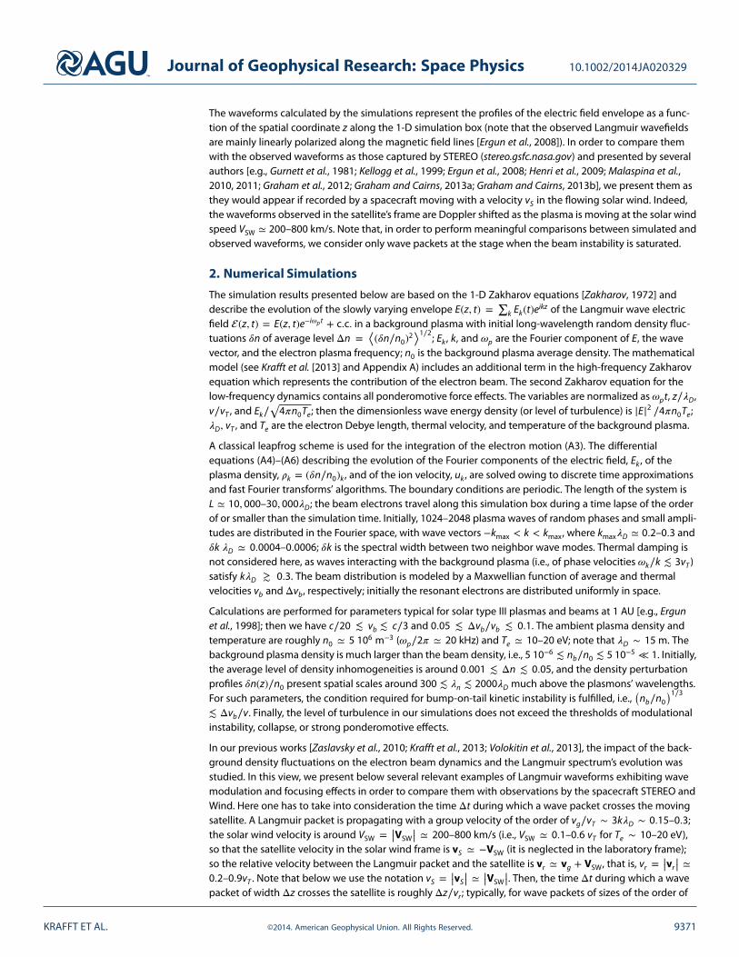
The variations of the field envelope profiles are very fast in the initial stage of the beam relaxation and maynot well correspond to what is actually observed after a longtime propagation of the beam. We study here-after the stage when the wave saturation is achieved and the beam relaxation process is well advanced. Atthis stage the velocity distribution f (v) presents a plateau with a more or less small gradient 𝜕f∕𝜕v ≳ 0.An overview of the Langmuir turbulence at this stage is shown in Figures 1–4. The first figure presents theelectric field envelopes’ profiles E(z), the wave energy density |E|2 (or level of turbulence), and the densityfluctuations 𝛿n∕n0 at time 𝜔pt = 30, 000, when the total spectral energy density W =
∑k |Ek|2 satu-
rates (Figure 3a) and the beam is almost fully relaxed (Figure 3b). The time evolution of f (v) in Figure 3bshows that the beam distribution broadens and diffuses to lower velocities, whereas a tail of acceleratedparticles appears at velocities v ≳ vb. Meanwhile, W grows (Figure 3a), reaching slowly saturation, whichis fully achieved when the beam decelerating velocity front has reached the thermal domain at v ≲ 3vT .One can observe in Figure 1 that the plasmon energy density |E|2 is concentrated in a few well-localizedpackets (Figure 1b) which, once formed, propagate with a roughly constant velocity but experience signifi-cant modifications in shape and amplitude, as shown by the variation with time of the wave energy profile(Figure 2). To complete the dynamics of the system, Figure 4 presents the high- and low-frequency spectra
ωpt
z/λ D
2
0 2 4
x 104
0
1
2
3
x 104
Figure 2. Profile of the wave energy |E|2 (z, t) as a function of time𝜔pt and space z∕𝜆D. Parameters are the same as in Figure 1.
at 𝜔pt = 30, 000; one observes that thehigh-frequency spectrum peaks nearkb𝜆D = vT∕vb ≃ 0.055, which is the wavenumber at the Landau resonance condition;it is broadened due to scattering and reflec-tions of Langmuir waves on the densityinhomogeneities, as shown by the presenceof counterpropagating waves with k < 0 (seealso Figure 4). The low-frequency spectrumreveals noise with rather broad peaks whichpossibly indicate the presence of wave-wavecoupling and electrostatic decay, which isrelated to the peak near k𝜆D ≃ −0.05 in theLangmuir spectrum of Figure 4a. The role ofthese processes will be considered in a forth-coming paper. Figures 1–4 correspond to aglobal view of the system, i.e., including the
KRAFFT ET AL. ©2014. American Geophysical Union. All Rights Reserved. 9372
Journal of Geophysical Research: Space Physics 10.1002/2014JA020329
0 2 4
x 104
0
1
2
3
4
5
x 10−4
ωpt
Σk
2
(a)
1020
30
0
5x 10⁴
0
0.2
0.4
v
(b)
ωpt
f(v)
Figure 3. Time evolution up to 𝜔pt = 54, 000 of (a) the total waveenergy density W =
∑k |Ek|2 and (b) the electron beam velocity
distribution f (v) (v is normalized by vT ). Parameters are the sameas in Figure 1.
evolution of all wave packets propagatingover the whole length of the simulationbox. Note that the amplitude of theLangmuir turbulence is small (|E|2
≲0.01) and,correspondingly, that the ponderomotiveforces are weak and that no cavity (densitydepletion) is formed in the plasma.
In the figures presented below, only localprocesses are studied, i.e., one only exam-ines instantaneous wave packets wherewave-wave interaction processes involv-ing ion-sound waves are very slow and donot play a significant role. This means thatwe study the time evolution of some chosenpart of the simulation box where we selectinstantaneous wave packets which arenot influenced by nonlinear effects dueto wave-wave coupling or modulationalinstability, for example. The profiles ofthe field envelopes calculated during thesimulations at times 𝜔pt=13, 000 and𝜔pt=25, 000 within the window[Lmin, Lmax]=[5000, 22, 000] are shown inFigures 5a and 5b for physical parametersclose to those of Figures 1–4. One can observethe presence of roughly four Langmuir wavepackets at 𝜔pt=13, 000, which keep more orless their identity during their propagationuntil 𝜔pt=25, 000, in spite of noticeable vari-ations of their forms. Figures 5c and 5d showthe corresponding waveforms that would beobserved onboard a spacecraft moving rel-
atively to the solar wind with the velocities vS = 0.2vT and vS = 0.6vT , respectively, supposing that theobservation starts when the satellite is located at the position zS = 16, 000𝜆D (indicated by an upward ver-tical line in Figure 5a) and finishes when it arrives at z = 13, 600𝜆D or at z = 8800𝜆D, for vS = 0.2vT andvS = 0.6vT , respectively (the final positions are indicated by downward lines in Figure 5a). Both waveformsin Figures 5c and 5d reveal clumpy features with beatings, which are typical of STEREO records; the wave-form observed at vS = 0.2vT (Figure 5c) corresponds roughly to the part of the waveform at vS = 0.6vT
(Figure 5d) extending from t ≃ 13, 000𝜔−1p up to t ≃ 18, 000𝜔−1
p . So it appears that the variation of the satel-lite velocity—i.e., of the solar wind speed or of its temperature—does not modify strongly the appearanceof the successive clumps of the waveform (that obviously is not the case for the initial satellite position andthe initial observation time). Note that, for lower satellite velocities, fine structures as beatings, for example,appear more clearly, with a better resolution. Then, some remarks can be formulated. First, the observedwaveforms (Figures 5c and 5d) differ noticeably from the instantaneous ones (Figures 5a and 5b), whatclearly corresponds to the modification of the wave packets’ profiles during the time of observation. Second,the features of the observed waveforms depend significantly on the spacecraft’s initial location, but a signif-icant variation of the satellite velocity does not distort the registration of the wave packets. However, this istrue only if the wave packets propagate rather stably during the observation time; if they are strongly modi-fied by nonlinear effects during the observation time, this last conclusion may become false and a variationof vS can modify essentially the main features of the waveform. Third, the observed waveforms present char-acteristics similar to those recorded in the solar wind by the Wind and STEREO spacecraft (see, for example,and among others, Malaspina et al. [2010, Figure 1b] and Malaspina et al. [2011, Figure 2a]).
For the same parameters and the same train of Langmuir packets as in Figures 5a–5d, but for a differenttime of observation and satellite location—with the same spacecraft velocity vS = 0.6vT —one observes
KRAFFT ET AL. ©2014. American Geophysical Union. All Rights Reserved. 9373

Journal of Geophysical Research: Space Physics 10.1002/2014JA020329
−0.2 −0.1 0 0.1 0.2
10−6
10−4
10−2
kλD
k
(a)
−0.2 −0.1 0 0.1 0.2
10−5
100
kλD
(b)
Figure 4. Spectra at 𝜔pt = 30, 000 and in logarithmic scale of (a)the Langmuir waves and (b) the low-frequency density fluctua-tions; Ek and 𝛿nk∕n0 are the Fourier components of E and 𝛿n∕n0.Parameters are the same as in Figure 1.
a totally different picture, as revealed byFigure 6a which shows an observed waveformappearing as an isolated packet containinga quasi-symmetric modulation pattern. Suchstructures have been observed, for exam-ple, by Ergun et al. [2008, Figure 3a], Grahamand Cairns [2013b, Figure 8a], and Henri et al.[2009, Figure 3c]. Note also that for the case oftype III solar bursts, the Langmuir waves arepropagating in the solar wind flow direction.At the foreshock, Langmuir waves propa-gate opposite to the solar wind; then, thespacecraft velocity in the solar wind frame isvS ≃VSW, but its modulus lies roughly withinthe same range of vS values as used above.Conclusions concerning the influence ofthe satellite velocity variation on the wave-forms are similar as for the case of type IIIsolar bursts.
Note that in most cases the solar wind flowand the ambient magnetic field are notaligned, as supposed in the present 1-D study.However, if one can neglect the componentof the electric field E⊥ perpendicular to themagnetic field with respect to the parallelone Ez , as it is possible for around 70% ofthe events, a nonvanishing angle 𝜃 betweenthe magnetic field and the solar wind flowwill only have an incidence on the satel-lite velocity, whose absolute value shoulddecrease when 𝜃 increases. Figure 6b showsthe observed waveform calculated for the
0.5 1 1.5 2
x 104
−0.1
0
0.1
Re(
E)
z/λD
ωpt=25000
(b)
0.5 1 1.5 2
x 104
−0.05
0
0.05
Re(
E)
z/λD
ωpt=13000
(a)
1.4 1.6 1.8 2 2.2 2.4
x 104
−0.05
0
0.05
t
ES
vS=0.6*v
T
(d)
1.4 1.6 1.8 2 2.2 2.4
x 104
−0.05
0
0.05
t
ES
vS=0.2*v
T
(c)
Figure 5. (a and b) Instantaneous electric field spatial profiles at times 𝜔pt = 13, 000 and 𝜔pt = 25, 000, within the sub-box [Lmin, Lmax] = [5000, 22, 000]. (c and d) Corresponding waveforms which would be observed by a satellite movingat velocity vS (of modulus vS) and starting at zS = 16, 000𝜆D at time 𝜔pt = 13, 000; the position zS is indicated by anupward dotted vertical line in Figure 5a; the final positions of the satellite moving at the velocities vS = 0.2vT (Figure 5c)and vS = 0.6vT (Figure 5d) are marked by downward dotted vertical lines in Figure 5a; ES is the electric field amplitudemeasured by the virtual spacecraft (normalized as the field E), and t is the time in units of 𝜔−1
p . Physical parameters arethe same as in Figure 1.
KRAFFT ET AL. ©2014. American Geophysical Union. All Rights Reserved. 9374

Journal of Geophysical Research: Space Physics 10.1002/2014JA020329
1.4 1.6 1.8 2 2.2 2.4
x 104
−0.05
0
0.05
t
ES
vS=0.01*v
T(b)
2.5 2.6 2.7 2.8 2.9 3
x 104
−0.05
0
0.05
t
ES
vS=0.6*v
T(a)
Figure 6. (a) Waveform observed at vS = 0.6vT for the same con-ditions as in Figures 5a–5d but with 25, 000 < 𝜔pt < 30, 000 andzS = 12, 000𝜆D. (b) Waveform observed for the same conditions asin Figures 5a–5d but for vS = 0.01vT . Physical parameters are thesame as in Figure 1.
same conditions as in Figure 5, but for a muchsmaller velocity vS = 0.01vT . The same qual-itative observations can be provided: even asignificant decrease of the satellite velocitydoes not distort the recorded waveform. Onthe other hand, if the perpendicular compo-nent of the electric field cannot be neglected,we have to take care that, during its obser-vation time Δt, the satellite should travelwithin the perpendicular spatial extent l⊥of the wave packet. Taking into account thatthe length lz of the Langmuir packet alongthe magnetic field is typically around 10 kmand that, according to the fact that waves arequasi-potential, we have Ez∕E⊥∼ l⊥∕lz with, for70% of cases, Ez∕E⊥∼10 or less (i.e., l⊥∼10lz
or more), the above condition can be writ-ten as |VSW sin𝜃| Δt ≪ 10lz , which gives fortypical values (VSW ∼500 km/s, Δt ∼ 0.05 s,lz ∼10 km) that |sin𝜃|≪ 4, condition whichis always fulfilled. In all such cases, our 1-Dmodeling can thus be applied. When the ratioEz∕E⊥ is smaller and the perpendicular field
component cannot be neglected, i.e., Ez∕E⊥∼3, the condition is |sin𝜃| ≪ 1, which continues to be true if 𝜃is roughly less than 20◦.
A next example is shown by Figure 7 for a denser beam, which presents in the same form as Figure 5 twoinstantaneous with their corresponding observed waveforms, for the velocities vS = 0.3vT and vS = 0.6vT ,respectively. The same remarks can be done as above for Figure 5. Moreover, the observed waveform forvS = 0.6vT (and also vS ≳ 0.6vT ) reproduces more or less accurately the structures of the instantaneouswave packets (compare the instantaneous wave packets between z = 7000𝜆D and z ≃ 20, 000𝜆D with theobserved wave packets between 𝜔pt ≃ 18, 000 and 𝜔pt ≃ 30, 000). Structures revealed by these waveformsresemble to the observations reported, for example, by Graham and Cairns [2013b, Figure 19a] and Gurnettet al. [1981, Figure 7b].
1 1.5 2 2.5
x 104
−0.05
0
0.05
Re(
E)
z/λD
ωpt=30000
(b)
1 1.5 2 2.5
x 104
−0.04−0.02
00.020.04
Re(
E)
z/λD
ωpt=18000
(a)
1.8 2 2.2 2.4 2.6 2.8 3
x 104
−0.05
0
0.05
t
ES
vS=0.6*v
T
(d)
1.8 2 2.2 2.4 2.6 2.8 3
x 104
−0.04
−0.02
0
0.02
0.04
t
ES
vS=0.3*v
T
(c)
Figure 7. (a and b) Instantaneous electric field profiles at times 𝜔pt = 18, 000 and t = 30, 000, within the subbox[Lmin, Lmax] = [7000, 25, 000]. (c and d) Corresponding waveforms which would be observed by a satellite moving atvelocity vS and starting at zS = 20, 000𝜆D at time 𝜔pt = 18, 000; the position zS is indicated by an upward dottedvertical line in Figure 7a; the final positions of the virtual satellite moving at the velocities vS = 0.3vT (Figure 7c) andvS = 0.6vT (Figure 7d) are marked by downward dotted vertical lines in Figure 7a. Main parameters are the following:nb∕n0 = 5 10−5, vb = 18vT , and Δn ≃ 0.01.
KRAFFT ET AL. ©2014. American Geophysical Union. All Rights Reserved. 9375
Journal of Geophysical Research: Space Physics 10.1002/2014JA020329
0.5 1 1.5
x 104
−0.1
0
0.1
Re(
E)
z/λD
ωpt=14000
(b)
0.5 1 1.5
x 104
−0.1
0
0.1
Re(
E)
z/λD
ωpt=5600
(a)
6000 8000 10000 12000 14000−0.1
0
0.1
t
E S
vS=0.35*v
T
(d)
6000 8000 10000 12000 14000−0.1
0
0.1
t
E S
vS=0.1*v
T
(c)
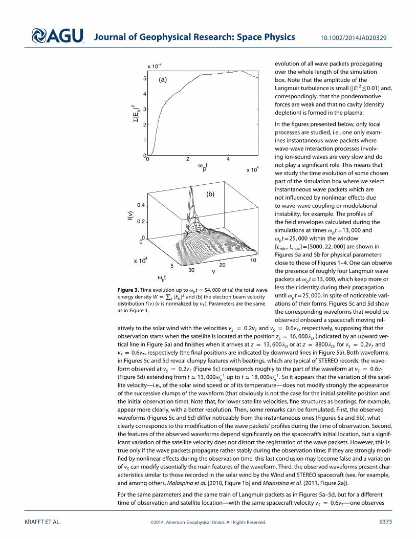
Figure 8. (a and b) Instantaneous electric field profiles at times 𝜔pt=5600 and 𝜔pt=14, 000, in the subbox[Lmin, Lmax] = [3000, 18, 000]. (c and d) Corresponding waveforms which would be observed by a satellite moving atvelocity vS and starting at zS = 7200𝜆D (upward dotted vertical line in Figure 8a) at time 𝜔pt = 5600; the final positionsof the satellite moving at the velocities vS = 0.1vT (Figure 8c) and vS = 0.35vT (Figure 8d) are marked by downwarddotted vertical lines in Figure 8a. Main parameters are the following: nb∕n0 = 10−5, vb = 18vT , and Δn ≃ 0.01.
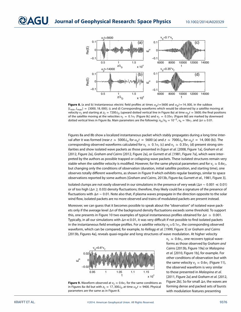
Figures 8a and 8b show a localized instantaneous packet which stably propagates during a long time inter-val after it was formed (near z ≃ 5000𝜆D for 𝜔pt = 5600 (a) and z ≃ 7000𝜆D for 𝜔pt = 14, 000 (b)). Thecorresponding observed waveforms calculated for vS ≃ 0.1vT (c) and vS ≃ 0.35vT (d) present strong sim-ilarities and show isolated wave packets as those presented in Ergun et al. [2008, Figure 1a], Graham et al.[2012, Figure 2a], Graham and Cairns [2012, Figure 2a], or Gurnett et al. [1981, Figure 7a], which were inter-preted by the authors as possible trapped or collapsing wave packets. These isolated structures remain verystable when the satellite velocity is modified. However, for the same physical parameters and for vS ≃ 0.6vT ,but changing only the conditions of observation (duration, initial satellite position, and starting time), oneobserves totally different waveforms, as shown in Figure 9 which exhibits regular beatings, similar to spaceobservations reported by some authors [Graham and Cairns, 2013b, Figure 6a; Gurnett et al., 1981, Figure 3].
Isolated clumps are not easily observed in our simulations in the presence of very weak (Δn ∼ 0.001 ≪ 0.01)or of too high (Δn ≳ 0.03) density fluctuations; therefore, they likely could be a signature of the presence offluctuations with Δn ∼ 0.01. Note also that, if plasma waves propagate in the direction opposite to the solarwind flow, isolated packets are no more observed and trains of modulated packets are present instead.
Moreover, we can guess that it becomes possible to speak about the “observation” of isolated wave pack-ets only if the average level Δn of the background density fluctuations exceeds some threshold. To supportthis, one presents in Figure 10 two examples of typical instantaneous profiles obtained for Δn ≃ 0.001.Typically, in all our simulations with Δn≪0.01, it was very difficult if not possible to find isolated packetsin the instantaneous field envelope profiles. For a satellite velocity vS ≃0.1vT , the corresponding observedwaveform, which can be compared, for example, to Kellogg et al. [1999, Figure 3] or Graham and Cairns[2013b, Figures 4a], reveals quasi-regular and long structures of wave modulation. At higher velocity
0.95 1 1.05 1.1 1.15
x 104
−0.02
0
0.02
t
ES
vS=0.6*v
T
Figure 9. Waveform observed at vS = 0.6vT for the same conditions asin Figures 8a–8d but with zS = 17, 300𝜆D at time 𝜔pt = 9400. Physicalparameters are the same as in Figure 8.
vS ≃ 0.6vT , one recovers typical wave-forms as those observed by Graham andCairns [2013b, Figure 19a] or Malaspinaet al. [2010, Figure 1b], for example. Forother conditions of observation but withthe same velocity vS ≃ 0.6vT (Figure 11),the observed waveform is very similarto those presented in Malaspina et al.[2011, Figure 2a] and Graham et al. [2012,Figure 2b]. So for small Δn, the waves areforming dense and packed sets of burstswith modulation features presenting
KRAFFT ET AL. ©2014. American Geophysical Union. All Rights Reserved. 9376
Journal of Geophysical Research: Space Physics 10.1002/2014JA020329
0 1000 2000 3000 4000 5000−0.05
0
0.05
Re(
E)
z/λD
ωpt=21000
(b)
0 1000 2000 3000 4000 5000
−0.05
0
0.05
Re(
E)
z/λD
ωpt=17000
(a)
1.7 1.8 1.9 2 2.1
x 104
−0.05
0
0.05
t
ES
vS=0.6*v
T
(d)
1.7 1.8 1.9 2 2.1
x 104
−0.05
0
0.05
t
ES
vS=0.1*v
T
(c)
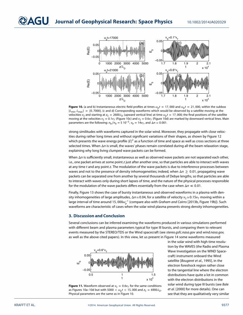
Figure 10. (a and b) Instantaneous electric field profiles at times 𝜔pt = 17, 000 and 𝜔pt = 21, 000, within the subbox[Lmin, Lmax] = [0, 7000]. (c and d) Corresponding waveforms which would be observed by a satellite moving at thevelocities vS and starting at zS = 2600𝜆D (upward vertical line) at time 𝜔pt = 17, 000; the final positions of the satellitemoving at the velocities vS = 0.1vT (Figure 10c) and vS = 0.6vT (Figure 10d) are marked by downward vertical lines. Mainparameters are the following: nb∕n0 = 5 10−5, vb = 14vT , and Δn ≃ 0.001.
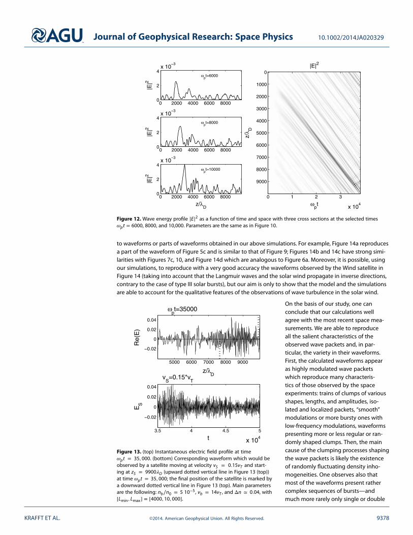
strong similitudes with waveforms captured in the solar wind. Moreover, they propagate with close veloc-ities during rather long times and without significant variations of their shapes, as shown by Figure 12which presents the wave energy profile |E|2 as a function of time and space as well as cross sections at threeselected times. When Δn is small, the waves’ phases remain correlated during all the beam relaxation stage,explaining why long living clumped wave packets can be formed.
When Δn is sufficiently small, instantaneous as well as observed wave packets are not separated each other,i.e., one packet arrives at some point z just after another one, so that particles are able to interact with wavesat any time t and any point z. The modulation of the wave packets is due to interference processes betweenwaves and not to the presence of density inhomogeneities; indeed, when Δn ≳ 0.01, propagating wavepackets can be separated one from another by several thousands of Debye lengths, so that particles are ableto interact with waves only during short lapses of time, and the nature of the physical processes responsiblefor the modulation of the wave packets differs essentially from the case when Δn ≪ 0.01.
Finally, Figure 13 shows the case of bursty instantaneous and observed waveforms in a plasma with den-sity inhomogeneities of large amplitudes, Δn≃0.04, for a satellite of velocity vS ≃0.15vT moving within alarge interval of time around 15, 000𝜔−1
p (compare also with Graham and Cairns [2013b, Figure 19b]). Suchwaveforms are characteristic of cases when the solar wind plasma presents strong density inhomogeneities.
3. Discussion and Conclusion
Several conclusions can be inferred examining the waveforms produced in various simulations performedwith different beam and plasma parameters typical for type III bursts, and comparing them to relevantevents measured by the STEREO/TDS or the Wind spacecraft (see stereo.gsfc.nasa.gov and wind.nasa.gov,as well as the above cited papers). In this view, let us present in Figure 14 some waveforms measured
0.5 1 1.5
x 104
−0.05
0
0.05
t
ES
vS=0.6*v
T
Figure 11. Waveform observed at vS = 0.6vT for the same conditionsas Figures 10a–10d but with 5000 < 𝜔pt < 15, 000 and zS = 6900𝜆D .Physical parameters are the same as in Figure 10.
in the solar wind with high time resolu-tion by the WAVES (the Radio and PlasmaWave Investigation on the WIND Space-craft) instrument onboard the Windsatellite [Bougeret et al., 1995], in theelectron foreshock region rather closeto the tangential line where the electrondistributions have quite a lot in commonwith the electron distributions in thesolar wind during type III bursts (see Baleet al. [2000] for more details). One cansee that they are qualitatively very similar
KRAFFT ET AL. ©2014. American Geophysical Union. All Rights Reserved. 9377
Journal of Geophysical Research: Space Physics 10.1002/2014JA020329
0 2000 4000 6000 80000
2
4x 10
−3
2
ωpt=6000
0 2000 4000 6000 80000
2
4x 10
−3
2
ωpt=8000
0 2000 4000 6000 80000
2
4x 10
−3
2
z/λD
ωpt=10000
ωpt
z/λ D
2
0 1 2 3
x 104
0
1000
2000
3000
4000
5000
6000
7000
8000
9000
Figure 12. Wave energy profile |E|2 as a function of time and space with three cross sections at the selected times𝜔pt = 6000, 8000, and 10,000. Parameters are the same as in Figure 10.
to waveforms or parts of waveforms obtained in our above simulations. For example, Figure 14a reproducesa part of the waveform of Figure 5c and is similar to that of Figure 9; Figures 14b and 14c have strong simi-larities with Figures 7c, 10, and Figure 14d which are analogous to Figure 6a. Moreover, it is possible, usingour simulations, to reproduce with a very good accuracy the waveforms observed by the Wind satellite inFigure 14 (taking into account that the Langmuir waves and the solar wind propagate in inverse directions,contrary to the case of type III solar bursts), but our aim is only to show that the model and the simulationsare able to account for the qualitative features of the observations of wave turbulence in the solar wind.
5000 6000 7000 8000 9000
−0.02
0
0.02
0.04
Re(
E)
z/λD
ωpt=35000
3.5 4 4.5 5
x 104
−0.02
0
0.02
0.04
t
ES
vS=0.15*v
T
Figure 13. (top) Instantaneous electric field profile at time𝜔pt = 35, 000. (bottom) Corresponding waveform which would beobserved by a satellite moving at velocity vS = 0.15vT and start-ing at zS = 9900𝜆D (upward dotted vertical line in Figure 13 (top))at time 𝜔pt = 35, 000; the final position of the satellite is marked bya downward dotted vertical line in Figure 13 (top). Main parametersare the following: nb∕n0 = 5 10−5, vb = 14vT , and Δn ≃ 0.04, with[Lmin, Lmax] = [4000, 10, 000].
On the basis of our study, one canconclude that our calculations wellagree with the most recent space mea-surements. We are able to reproduceall the salient characteristics of theobserved wave packets and, in par-ticular, the variety in their waveforms.First, the calculated waveforms appearas highly modulated wave packetswhich reproduce many characteris-tics of those observed by the spaceexperiments: trains of clumps of variousshapes, lengths, and amplitudes, iso-lated and localized packets, “smooth”modulations or more bursty ones withlow-frequency modulations, waveformspresenting more or less regular or ran-domly shaped clumps. Then, the maincause of the clumping processes shapingthe wave packets is likely the existenceof randomly fluctuating density inho-mogeneities. One observes also thatmost of the waveforms present rathercomplex sequences of bursts—andmuch more rarely only single or double
KRAFFT ET AL. ©2014. American Geophysical Union. All Rights Reserved. 9378

Journal of Geophysical Research: Space Physics 10.1002/2014JA020329
Figure 14. (a–d) Waveforms measured at 20 April 1996 by the Wind satellite in the electron foreshock region rather closeto the tangential line where electron distributions have quite a lot in common with the electron distributions in the solarwind during type III bursts (see also Bale et al. [2000] for more details); the amplitude E of the electric field envelope(in mV/m) is displayed as a function of the time t in ms.
humps—and that waves are rather rarely trapped in density fluctuations, this occurring mainly when theaverage amplitude of density inhomogeneities is high (roughly Δn ≳ 0.05).
The organization of the waveforms into focused packets begins at early stages of the system’s evolution,even before the growth of waves due to beam instability has reached an appreciable strength, indicat-ing that nonlinear kinematic effects involving scattering and reflection are playing a significant role. Nophenomena such as collapse or modulational instability are observed for the parameters used and the pon-deromotive effects are shown to be weak, supposed that the beam density is sufficiently weak (what isthe case here, see parameters above). As a consequence, many characteristic features of the wave packets’modulation are visible even in the absence of nonlinear effects such as wave-wave coupling, modulationalinstability, and collapse; the nonlinear processes are not the cause of the clumpy nature of the waveforms.However, they can modify them and even enhance the focusing processes which are shaping them (thistopics will be discussed in detail in a forthcoming paper).
It is likely that the observation of highly localized and isolated wave packets is possible only if Δn exceedssome threshold. Moreover, the authors believe that the observation of such structures can be a signaturefor the presence of nonnegligible (but also not too high) levels of density fluctuations, i.e., Δn∼0.01. Wealso see that variations of the solar wind speed do not modify essentially the characteristic features of theobserved waveforms reconstructed using the instantaneous profiles.
The authors believe that the clumping processes observed should be mainly due to nonlinear kinematiceffects of wave propagation, reflection, and scattering in randomly fluctuating density profiles, which areinfluenced by the beam instability during the stage of linear wave growth. The wave spectra show that,during the evolution, reflected waves are generated after some time (see, e.g., Figure 4) and that the waveenergy has tendency to focus near the wells’ reflection points (see Figure 1b). This focusing is shown tooccur with and without the beam, but it can be enhanced by the presence of the beam. Indeed, the beaminstability plays an important role; after waves with resonant velocities v𝜑 = 𝜔k∕k < vb have gained energyfrom the beam particles with velocities v < vb via the beam instability developing at 𝜕f∕𝜕v > 0, theycan transfer part of their energy to waves with v𝜑>vb, as a result of their scattering by the density inhomo-geneities, the random modification of their phase velocities and their resonance conditions with the beamelectrons. When Δn is sufficiently large (Δn≳𝛼k2𝜆2
D ∼0.01 Krafft et al. [2013]), the Langmuir spectrum is flat-tened in the asymptotic stage. It is not the case when Δn is very small (Δn ≪ 𝛼k2𝜆2
D Krafft et al. [2013]).
KRAFFT ET AL. ©2014. American Geophysical Union. All Rights Reserved. 9379

Journal of Geophysical Research: Space Physics 10.1002/2014JA020329
In their turn, these waves can be submitted to Landau damping and thus transfer part of their energy toaccelerate particles with velocities v > vb. During these processes, the effective growth rate of each waveis changed randomly, and this organizes the modulation of the waveforms and modifies the number, theshapes, and the distribution of the clumps along the profiles. The combinations of all the mentioned effectscontribute to create various types of modulations of the wave packet, its clumpiness indicating how thewave energy is distributed and more or less concentrated in localized spatial regions.
However, modulation effects shaping the Langmuir packets appear also in the presence of very small aver-age levels of density inhomogeneities as the result of beatings between waves. Note also that other effectscan influence the modulation effects structuring the waveforms: resonant wave-wave coupling betweenLangmuir wave packets and low-frequency (ion acoustic) waves, modulational instability where pondero-motive effects are strong, and collapse effects with further breaking into trains of ion acoustic solitons. Thefirst one will be discussed in a forthcoming paper, particularly its influence on the modulation of the wavepackets. The two other effects are usually not present in our simulations, taking into account the parame-ters chosen, so that their impact is not determinant on the focusing processes observed in our conditions;indeed, the presence of inhomogeneities decreases the maximum of wave energy reached which is thusdecreasing below the modulational instability and collapse thresholds.
Appendix A: Theoretical Model
The 1-D theoretical model describes the self-consistent interaction of Langmuir waves with electron beamsin plasmas with randomly varying density inhomogeneities. The dynamics of Langmuir and ion soundwaves is calculated using the two Zakharov’s equations [Zakharov, 1972] where a source term is added tomodel the beam. As shown in a previous paper [Krafft et al., 2013], these equations can be written as
i𝜕E𝜕t
+3𝜆2
D
2𝜔p
𝜕2E𝜕z2
− 𝜔p𝛿n2n0
E = 4𝜋ienb
∑k
𝜔p
k1N
∑p
ei𝜔pt−ikzp eikz, (A1)
(𝜕2
𝜕t2− c2
s𝜕2
𝜕z2
)𝛿nn0
= 𝜕2
𝜕z2
|E|2
16𝜋min0, (A2)
where z is the coordinate along the ambient magnetic field B0; 𝜔p and 𝜆D are the electron plasma frequencyand Debye length; k is the wave number of the Langmuir wave of frequency 𝜔k ≃ 𝜔p + 3𝜔pk2𝜆2
D∕2; = Re(E (z, t) e−i𝜔pt) is the electric field, and E (z, t) is its slowly varying envelope; 𝛿n is the low-frequencydensity perturbation; mi and me are the ion and electron masses; −e < 0 is the electron charge; nb is thebeam density; Ti and Te are the ion and electron temperatures, which are supposed to satisfy the conditionTi ≪ Te; cs =
√(Te + 3Ti)∕mi is the ion acoustic velocity; zp is the position of the particle p; and N is the
number of macroparticles, i.e., the number of resonant electrons.
The model divides the total particle distribution in two groups: (i) the background plasma whose parti-cles interact nonresonantly with the waves, and (ii) the beam particles which exchange resonantly withthe waves significant amounts of energy and momentum [e.g., O’Neil et al., 1971; Volokitin and Krafft, 2004;Zaslavsky et al., 2006; Krafft et al., 2005, 2006; Krafft and Volokitin, 2010; Krafft et al., 2010; Zaslavsky et al.,2007; Krafft and Volokitin, 2013]. The first group of electrons supports the wave dispersion and its dynamicsis modeled using the dielectric constant in the frame of a linear approach (see also the beam source termin (A1)). On another hand, the resonant electrons of velocity v exchange momentum and energy with theplasma waves at the Landau resonances 𝜔k ≃ 𝜔p ≃ kv. Their dynamics is calculated by solving the Newtonequations. Such approach leads to a drastic reduction of the number of macroparticles required in the cal-culations, giving the possibility to study the microscopic beam dynamics and the Langmuir turbulence overlong periods of time. Nevertheless, it is required the resonant particles’ density nb to be much less than theambient plasma density, i.e., nb ≪ n0.
The Newton equations for the N particles p have to be added to equations (A1) and (A2)
me
dvp
dt= −e(zp, t) = −eRe
(∑k
Ekeikzp−i𝜔k t
),
dzp
dt= vp, (A3)
KRAFFT ET AL. ©2014. American Geophysical Union. All Rights Reserved. 9380
Journal of Geophysical Research: Space Physics 10.1002/2014JA020329
where vp is the velocity of the electron p; Ek is the Fourier component of E
Ek(t) = ∫L
0E(z, t)e−ikz dz
L,
where L = N∕nb is the size of the system. Rewriting equation (A1) in the k space, one obtains that
i(𝜕
𝜕t− 𝛾
(e)k
)Ek = 3
2𝜔pk2𝜆2
DEk +𝜔p
2(𝜌E)k + i
4𝜋e𝜔pnb
kJk, (A4)
where 𝜌 = 𝛿n∕n0; a kinetic damping factor 𝛾 (e)k = −Im𝜀(e)k ∕(𝜕Re𝜀(e)k ∕𝜕𝜔k) (where the superscript (e) refers to
electrons) is added eventually in (A4) in order to take into account the damping of the plasma waves wheninteracting with thermal particles or with nonthermal electrons of the background plasma distribution, asfor example non-Maxwellian tails.
The Fourier transforms of equation (A2) and of the plasma continuity equation lead to the followingexpressions (ion damping is not included)
𝜕
𝜕t𝜌k = ikcsuk, (A5)
𝜕uk
𝜕t= ikcs
(𝜌k +
(|E|2)k
16𝜋min0c2s
), (A6)
where vi and u = vi∕cs are the ion velocity and its normalized value. Equations (A4)–(A6) together withequation (A3) form the complete set of equations of our model.
ReferencesBale, S. D., D. E. Larson, R. P. Lin, P. J. Kellogg, K. Goetz, and S. J. Monson (2000), On the beam speed and wavenumber of intense electron
plasma waves near the foreshock edge, J. Geophys. Res., 105(A12), 27,353–27,367, doi:10.1029/2000JA900042.Bonnell, J., P. Kintner, J.-E. Wahlund, and J. A. Holtet (1997), Modulated Langmuir waves: Observations from Freja and Scifer, J. Geophys.
Res., 102(A8), 17,233–17,240, doi:10.1029/97JA01499.Boshuizen, C. R., I. H. Cairns, and P. A. Robinson (2004), Electric field distributions for Langmuir waves in planetary foreshocks, J. Geophys.
Res., 109, A08101, doi:10.1029/2004JA010408.Bougeret, J.-L., et al. (1995), WAVES: The radio and plasma wave investigation on the WIND spacecraft, Space Sci. Rev., 71, 231–263,
doi:10.1007/BF00751331.Bougeret, J.-L., et al. (2008), S/waves: The radio and plasma wave investigation on the Stereo mission, Space Sci. Rev., 136, 487–529,
doi:10.1007/s11214-007-9298-8.Celnikier, L. M., C. C. Harvey, R. Jegou, P. Moricet, and M. Kemp (1983), A determination of the electron density fluctuation spectrum in
the solar wind, using the ISEE propagation experiment, Astron. Astrophys., 126, 293–298.Celnikier, L. M., L. Muschietti, and M. V. Goldman (1987), Aspects of interplanetary plasma turbulence, Astron. Astrophys., 181, 138–154.Ergun, R. E., et al. (1998), Wind spacecraft observations of solar impulsive electron events associated with solar type III radio bursts,
Astrophys. J., 503(1), 435–445, doi:10.1086/305954.Ergun, R. E., et al. (2008), Eigenmode structure in solar-wind Langmuir waves, Phys. Rev. Lett., 101, 051,101, doi:10.1103/Phys-
RevLett.101.051101.Ginzburg, V., and V. Zheleznyakov (1958), On possible mechanisms of sporadic solar radio emission, Sov. Astron. AJ, 2, 653–668.Graham, D. B., and I. H. Cairns (2013a), Constraints on the formation and structure of Langmuir eigenmodes in the solar wind, Phys. Rev.
Lett., 111, 121,101, doi:10.1103/PhysRevLett.111.121101.Graham, D. B., and I. H. Cairns (2013b), Electrostatic decay of Langmuir/z-mode waves in type III solar radio bursts, J. Geophys. Res. Space
Physics, 118, 3968–3984, doi:10.1002/jgra.50402.Graham, D. B., I. H. Cairns, D. R. Prabhakar, R. E. Ergun, D. M. Malaspina, S. D. Bale, K. Goetz, and P. J. Kellogg (2012), Do Langmuir wave
packets in the solar wind collapse?, J. Geophys. Res., 117, A09107, doi:10.1029/2012JA018033.Gurnett, D., and R. Anderson (1976), Electron plasma oscillations associated with type III radio bursts, Science, 194(4270), 1159–1162,
doi:10.1126/science.194.4270.1159.Gurnett, D., G. Hospodarsky, W. Kurth, D. Williams, and S. Bolton (1993), Fine structure of Langmuir waves produced by a solar electron
event, J. Geophys. Res., 98(A4), 5631–5637, doi:10.1029/92JA02838.Gurnett, D. A., R. R. Anderson, F. L. Scarf, and W. S. Kurth (1978), The heliocentric radial variation of plasma oscillations associated with
type III radio bursts, J. Geophys. Res., 83, 4147–4152, doi:10.1029/JA083iA09p04147.Gurnett, D. A., J. E. Maggs, D. L. Gallagher, W. S. Kurth, and F. L. Scarf (1981), Parametric interaction and spatial collapse of beam-driven
Langmuir waves in the solar wind, J. Geophys. Res., 86(A10), 8833–8841, doi:10.1029/JA086iA10p08833.Gurnett, D. A., W. S. Kurth, R. R. Shaw, A. Roux, R. Gendrin, C. F. Kennel, F. L. Scarf, and S. D. Shawhan (1992), The Galileo plasma wave
investigation, Space Sci. Rev., 60, 341–355, doi:10.1007/BF00216861.Henri, P., C. Briand, A. Mangeney, S. D. Bale, F. Califano, K. Goetz, and M. Kaiser (2009), Evidence for wave coupling in type III emissions,
J. Geophys. Res., 114, A03103, doi:10.1029/2008JA013738.Hess, S. L. G., D. M. Malaspina, and R. E. Ergun (2011), Size and amplitude of Langmuir waves in the solar wind, J. Geophys. Res., 116,
A07104, doi:10.1029/2010JA016163.Hospodarsky, G., and D. Gurnett (1995), Beat-type Langmuir wave emissions associated with a type III solar radio bursts, Geophys. Res.
Lett., 22, 1161–1164, doi:10.1029/95GL00303.
AcknowledgmentsWe thank T. Dudok de Wit([email protected]) andV. Krasnoselskikh ([email protected]) for providing the data ofFigure 14, available at wind.nasa.gov.V.K. acknowledges the financial sup-port of the Centre National d’EtudesSpatiales (CNES) through the grant“Invited scientist STEREO S/WAVES.”This work was granted access to theHPC resources of IDRIS under theallocation 2013-i2013057017 madeby GENCI. This work has been donewithin the LABEX Plas@par projectand received financial state aid man-aged by the Agence Nationale de laRecherche, as part of the programme“Investissements d’avenir” underthe reference ANR-11-IDEX-0004-02.C.K. acknowledges the “ProgrammeNational Soleil Terre” (PNST) and theCentre National d’Etudes Spatiales(CNES, France).
Michael Balikhin thanks the reviewersfor their assistance in evaluatingthis paper.
KRAFFT ET AL. ©2014. American Geophysical Union. All Rights Reserved. 9381
Journal of Geophysical Research: Space Physics 10.1002/2014JA020329
Kellogg, P., K. Goetz, S. Monson, and S. Bale (1999), Langmuir waves in a fluctuating solar wind, J. Geophys. Res., 104(A8), 17069–17078,doi:10.1029/1999JA900163.
Kellogg, P. J. (1986), Observations concerning the generation and propagation of type III solar bursts, Astron. Astrophys., 169, 329–335.Kellogg, P. J., and T. S. Horbury (2005), Rapid density fluctuations in the solar wind, Ann. Geophys., 23, 3765–3773,
doi:10.5194/angeo-23-3765-2005.Kellogg, P. J., K. Goetz, S. J. Monson, S. D. Bale, M. J. Reiner, and M. Maksimovic (2009), Plasma wave measurements with STEREO
S/WAVES: Calibration, potential model, and preliminary results, J. Geophys. Res., 114, A02107, doi:10.1029/2008JA013566.Kojima, H., H. Furuya, H. Usui, and H. Matsumoto (1997), Modulated electron plasma waves observed in the tail lobe: Geotail waveform
observations, Geophys. Res. Lett., 24, 3049–3052, doi:10.1029/97GL03043.Krafft, C., and A. Volokitin (2006), Stabilization of the fan instability: Electron flux relaxation, Phys. Plasmas, 13, 122,301,
doi:10.1063/1.2372464.Krafft, C., and A. Volokitin (2010), Nonlinear fan instability of electromagnetic waves, Phys. Plasmas, 17, 102,303, doi:10.1063/1.3479829.Krafft, C., and A. Volokitin (2013), Nonturbulent stabilization of ion fluxes by the fan instability, Phys. Lett. A, 377, 1189–1198,
doi:10.1016/j.physleta.2013.03.011.Krafft, C., A. Volokitin, and A. Zaslavsky (2005), Saturation of the fan instability: Nonlinear merging of resonances, Phys. Plasmas, 12,
112309, doi:10.1063/1.2118727.Krafft, C., A. Volokitin, and A. Zaslavsky (2010), Nonlinear dynamics of resonant interactions between wave packets and particle
distributions with loss cone-like structures, Phys. Rev. E, 82(6), 066402, doi:10.1103/PhysRevE.82.066402.Krafft, C., A. S. Volokitin, and V. V. Krasnoselskikh (2013), Interaction of energetic particles with waves in strongly inhomogeneous solar
wind plasmas, Astrophys. J., 778, 111, doi:10.1088/0004-637X/778/2/111.Krasnoselskikh, V., V. V. Lobzin, K. Musatenko, J. Soucek, J. S. Pickett, and I. H. Cairns (2007), Beam-plasma interaction in randomly
inhomogeneous plasmas and statistical properties of small-amplitude Langmuir waves in the solar wind and electron foreshock,J. Geophys. Res., 112, A10109, doi:10.1029/2006JA012212.
Lin, R., W. Levedahl, W. Lotko, D. Gurnett, and F. Scarf (1986), Evidence for nonlinear wave-wave interaction in solar type III radio bursts,Astrophys. J., 308, 954–965, doi:10.1086/164563.
Lin, R. P., D. W. Potter, D. A. Gurnett, and F. L. Scarf (1981), Energetic electrons and plasma waves associated with a solar type III radioburst, Astrophys. J., 251, 364–373, doi:10.1086/159471.
Malaspina, D. M., and R. E. Ergun (2008), Observations of three-dimensional Langmuir wave structure, J. Geophys. Res., 113, A12108,doi:10.1029/2008JA013656.
Malaspina, D. M., P. J. Kellogg, S. D. Bale, and R. E. Ergun (2010), Measurements of rapid density fluctuations in the solar wind,Astrophys. J., 711, 322–327, doi:10.1088/0004-637X/711/1/322.
Malaspina, D. M., I. H. Cairns, and R. E. Ergun (2011), Dependence of Langmuir wave polarization on electron beam speed in type III solarradio bursts, Geophys. Res. Lett., 38, L13101, doi:10.1029/2011GL047642.
Mangeney, A., C. Salem, C. Lacombe, J. L. Bougeret, C. Perche, R. Manning, P. J. Kellogg, K. Goetz, S. J. Monson, and J.-M. Bosqued (1999),Wind observations of coherent electrostatic waves in the solar wind, Ann. Geophys., 17, 307–320, doi:10.1007/s00585-999-0307-y.
Melrose, D. B., G. A. Dulk, and I. H. Cairns (1986), Clumpy Langmuir waves in type III solar radio bursts, Astron. Astrophys., 163, 229–238.Muschietti, L., I. Roth, and R. Ergun (1994), Interaction of Langmuir wave packets with streaming electrons: Phase-correlation aspects,
Phys. Plasmas, 1, 1008–1024, doi:10.1063/1.870781.Muschietti, L., I. Roth, and R. E. Ergun (1995), Kinetic localization of beam-driven Langmuir waves, J. Geophys. Res., 100(A9), 17,481–17,490,
doi:10.1029/95JA00595.Nicholson, D. R., M. V. Goldman, P. Hoyng, and J. C. Weatherall (1978), Nonlinear Langmuir waves during type III solar radio bursts,
Astrophys. J., 223, 605–619, doi:10.1086/156296.Nulsen, A. L., I. H. Cairns, and P. A. Robinson (2007), Field distributions and shapes of Langmuir wave packets observed by Ulysses in an
interplanetary type III burst source region, J. Geophys. Res., 112, A05107, doi:10.1029/2006JA011873.O’Neil, T., J. Winfrey, and J. Malmberg (1971), Nonlinear interaction of a small cold beam and a plasma, Phys. Fluids, 14, 1204–1212.Robinson, P. A. (1992), Clumpy Langmuir waves in type III radio sources, Solar Phys., 139, 147–163, doi:10.1007/BF00147886.Robinson, P. A., A. J. Willes, and I. H. Cairns (1993), Dynamics of Langmuir and ion-sound waves in type III solar radio sources,
Astrophys. J., 408, 720–734, doi:10.1086/172632.Smith, D. F., and D. Sime (1979), Origin of plasma-wave clumping in type III solar radio burst sources, Astrophys. J., 233, 998–1004,
doi:10.1086/157463.Soucek, J., V. Krasnoselskikh, T. D. de Wit, J. Pickett, and C. Kletzing (2005), Nonlinear decay of foreshock Langmuir waves in the presence
of plasma inhomogeneities: Theory and Cluster observations, J. Geophys. Res., 110, A08102, doi:10.1029/2004JA010977.Thejappa, G., R. J. MacDowall, E. E. Scime, and J. E. Littleton (2003), Evidence for electrostatic decay in the solar wind at 5.2 au, J. Geophys.
Res., 108, A31139, doi:10.1029/2002JA009290.Volokitin, A., and C. Krafft (2004), Interaction of suprathermal electron fluxes with lower hybrid waves, Phys. Plasmas, 11(6), 3165–3176,
doi:10.1063/1.1715100.Volokitin, A., and C. Krafft (2012), Velocity diffusion in plasma waves excited by electron beams: A numerical experiment, Plasma Phys.
Contr. Fusion, 54(085002), doi:10.1088/0741-3335/54/8/085002.Volokitin, A., V. Krasnoselskikh, C. Krafft, and E. Kuznetsov (2013), Modelling of the beam-plasma interaction in a strongly inhomoge-
neous plasma, AIP Conf. Proc., 1539(1), 78–81, doi:10.1063/1.4810994.Zakharov, V. (1972), Collapse of Langmuir waves, Sov. Phys. JETP, 35(5), 908–914.Zaslavsky, A., C. Krafft, and A. Volokitin (2006), Stochastic processes of particle trapping and detrapping by a wave in a magnetized
plasma, Phys. Rev. E, 73(016406), doi:10.1103/PhysRevE.73.016406.Zaslavsky, A., C. Krafft, and A. Volokitin (2007), Loss-cone instability: Wave saturation by particle trapping, Phys. Plasmas, 14, 122302,
doi:10.1063/1.2799621.Zaslavsky, A., A. Volokitin, V. V. Krasnoselskikh, M. Maksimovic, and S. D. Bale (2010), Spatial localization of Langmuir waves generated
from an electron beam propagating in an inhomogeneous plasma: Applications to the solar wind, J. Geophys. Res., 115, A08103,doi:10.1029/2009JA014996.
KRAFFT ET AL. ©2014. American Geophysical Union. All Rights Reserved. 9382