wave scattering by inﬁnite cylindrical shell structures ......wave motion 38 (2003) 131–149 wave...

Wave Motion 38 (2003) 131–149

Wave scattering by infinite cylindrical shell structuressubmerged in a fluid medium

L. Godinho, A. Tadeu∗, F.J. BrancoDepartment of Civil Engineering, University of Coimbra, Polo II—Pinhal de Marrocos, 3030-290 Coimbra, Portugal

Received 27 June 2002; received in revised form 19 December 2002; accepted 4 February 2003

Abstract

This work analyzes the wave scattering by an elastic, fluid-filled, cylindrical shell structure submerged in a fluid mediumand subjected to the effect of a point pressure load placed inside or outside the cylindrical shell. The shell structures modeledhave constant cross-sections along their axis, corresponding to 2.5D problems. A Fourier transformation in the direction inwhich the geometry does not vary is applied to find the 3D field as the summation of the 2D solutions for different spatialwavenumbers.

The wave propagation patterns are analyzed for shell structures defined by two concentric or non-concentric cylindricalcircular surfaces. The boundary element method, formulated in the frequency domain, is used to calculate the dynamic responseof these systems when the shell is defined by non-concentric cylindrical circular surfaces, while analytical solutions are usedto compute the response when two concentric cylindrical circular surfaces define the shell structure. Different simulations areperformed for receivers placed at distinct positions, in order to study the normal modes excited at each load position withineach shell structure type. Both frequency and time solutions are obtained, in an attempt to obtain wave propagation featuresthat may be used as a basis for developing non-destructive testing techniques.© 2003 Elsevier Science B.V. All rights reserved.

1. Introduction

Wave propagation and vibration phenomena have interested researchers for many years. The particular case ofthe vibration of thin or thick shell structures has been analyzed using many different approaches, ranging fromanalytical to numerical methods. The latter are applicable to a wide range of situations, and allow the analysis ofphysical systems with different configurations.

The propagation of guided transient waves in the circumferential direction of annular structural components wasaddressed by Liu and Qu[1]. Their work used the eigenfunction expansion method to analyze a circular annuluswith null traction at the inner surface and subject to a time dependent transient excitation with different incidenceangles at the outer surface. This method allowed the contributions of the different eigenmodes to be separated,making it possible to identify the ones making more important contributions to the response. Chung and Lee[2]proposed a new conical ring element to be used in connection with the finite element method to analyze the free

∗ Corresponding author. Tel.:+351-239-797-204; fax:+351-239-797-190.E-mail address:[email protected] (A. Tadeu).

0165-2125/03/$ – see front matter © 2003 Elsevier Science B.V. All rights reserved.doi:10.1016/S0165-2125(03)00026-X

132 L. Godinho et al. / Wave Motion 38 (2003) 131–149

vibrations of nearly axisymmetric shell structures. The element proposed allowed the effect of a possible slight localdeviation from the pure axisymmetric form to be taken into account.

The free vibration of rings with profile variations in the circumferential direction was studied by Hwang et al.[3]. Their methodology was based on expressing the inner and the outer profiles as Fourier series, using an it-erative numerical procedure to determine the middle surface and thickness at each cross-section. Novozhilov’sthin shell theory is then used to model the deformation mechanics of the ring, and eigenfrequencies are deter-mined by the Rayleigh–Ritz method, together with a harmonic series description of the displacements. Severalcases were analyzed by Fox et al.[4] using this method, in which the inner and outer profiles are nominallycircular with various superimposed harmonic variations in radius. The most important causes of frequency split-ting were identified and highlighted. Later, the same method was used[5] to assess the vibration of ellipticalrings with a constant or variable cross-section, examining the effect of the aspect ratio of the ellipse and theinfluence of single harmonic perturbations of the ring profile on the frequency splitting of vibration modes.These results compared well with previously published results for aspect ratios close to unity. However, foraspect ratios significantly different from unity, the additional terms used by the authors increased theaccuracy.

When a fluid medium is present inside or outside the structure, more elaborate models that take into account thecoupling between the solid and the fluid should be used. Researchers proposed different models to solve problemsof this type. The wave scattering by submerged elastic circular cylindrical shells, filled with air, struck by planeharmonic acoustic waves was analyzed by Veksler et al.[6]. They used the standard resonance scattering theoryto study the modal resonances, focusing their investigation on the generation of bending waves. They concludedthat these waves could be generated when the relative thickness of the shell is not too great, and that the dispersioncurves of their phase velocity were limited by the dispersion curves of the free bending modes, when the density ofthe host fluid tends towards zero.

Bao et al.[7] addressed the existence of various types of circumferential waves and the repulsion of their dispersioncurves for the case of a submerged thin elastic circular fluid-filled cylindrical shell. Their study was based on ananalytical calculation of the partial-wave resonances in the acoustic scattering amplitude of a normally incidentplane wave.

Recent work by Maze et al.[8] presented a study on the various guided acoustic circumferential modes found ina water-filled tube. This work showed, both theoretically and experimentally, that structure waves are present insidea water-filled thin walled tube in vacuum. The group velocities for the first two coupled modes calculated by theauthors were in excellent agreement with experimental results.

In many cases, the shell structure may not be perfectly circular, and the interior and exterior surfaces may bedefined by two non-concentric circumferences. This deviation from a pure circular form, with constant thickness,introduces variations in the dynamic behavior of the structure. In the present paper, the authors analyze the 3D wavepropagation in the vicinity of a fluid-filled cylindrical shell structure, submerged in a continuous homogeneous fluidmedium. The full coupling between the external fluid, the elastic material and the internal fluid is taken into account.Two cross-sections are studied, corresponding to shells defined by two concentric or non-concentric circumferences.In both cases, the shell is assumed to be made of a homogeneous elastic material.

A 2.5D formulation was used, taking into account the full 3D nature of the problem. This formulation allowedthe authors to obtain 3D responses in the frequency domain as a discrete summation of the 2D solutions for differentaxial wavenumbers[9]. Analytical solutions are used to solve each of the 2D problems when the thickness of theshell wall is constant, and the boundary element method (BEM) is applied to obtain the response when the cylindricalshell is not perfect. Pressure variations in the fluid medium that fills the shell and the dependence of the differentnormal modes on the position of the source and geometry of the cross-section are analyzed. A better understandingof the behavior of the dynamic system is gained from the time domain responses, which are obtained using inverseFourier transforms.

First, this work describes the 2.5D formulation of the scattering problem, the analytical and the BEM frequencysolutions. Then, the BEM solution is validated against the analytical solution. Next, the process used to computetime domain results is described. Finally, a set of numerical applications is presented, showing how an infinite

L. Godinho et al. / Wave Motion 38 (2003) 131–149 133

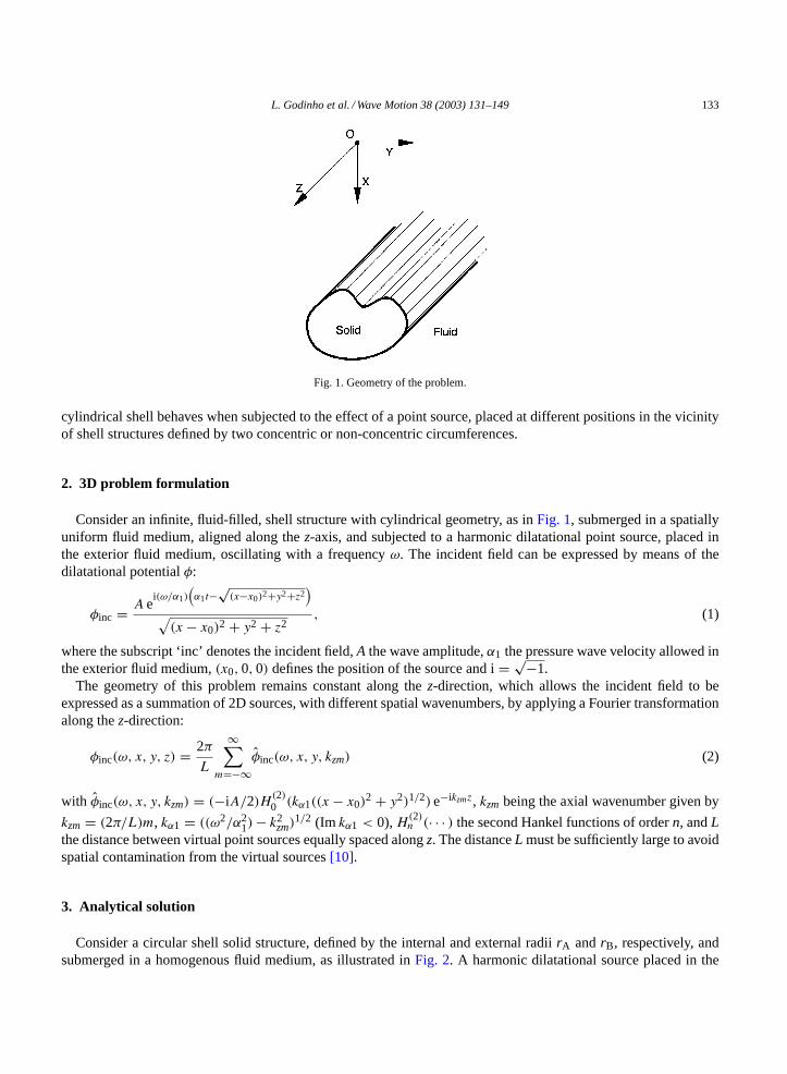
Fig. 1. Geometry of the problem.

cylindrical shell behaves when subjected to the effect of a point source, placed at different positions in the vicinityof shell structures defined by two concentric or non-concentric circumferences.

2. 3D problem formulation

Consider an infinite, fluid-filled, shell structure with cylindrical geometry, as inFig. 1, submerged in a spatiallyuniform fluid medium, aligned along thez-axis, and subjected to a harmonic dilatational point source, placed inthe exterior fluid medium, oscillating with a frequencyω. The incident field can be expressed by means of thedilatational potentialφ:

φinc = Aei(ω/α1)

(α1t−

√(x−x0)

2+y2+z2)

√(x − x0)2 + y2 + z2

, (1)

where the subscript ‘inc’ denotes the incident field,A the wave amplitude,α1 the pressure wave velocity allowed inthe exterior fluid medium,(x0,0,0) defines the position of the source and i= √−1.

The geometry of this problem remains constant along thez-direction, which allows the incident field to beexpressed as a summation of 2D sources, with different spatial wavenumbers, by applying a Fourier transformationalong thez-direction:

φinc(ω, x, y, z) = 2π

L

∞∑m=−∞

φinc(ω, x, y, kzm) (2)

with φinc(ω, x, y, kzm) = (−iA/2)H(2)0 (kα1((x − x0)

2 + y2)1/2)e−ikzmz, kzm being the axial wavenumber given by

kzm = (2π/L)m, kα1 = ((ω2/α21)− k2

zm)1/2 (Im kα1 < 0),H(2)

n (· · · ) the second Hankel functions of ordern, andLthe distance between virtual point sources equally spaced alongz. The distanceL must be sufficiently large to avoidspatial contamination from the virtual sources[10].

3. Analytical solution

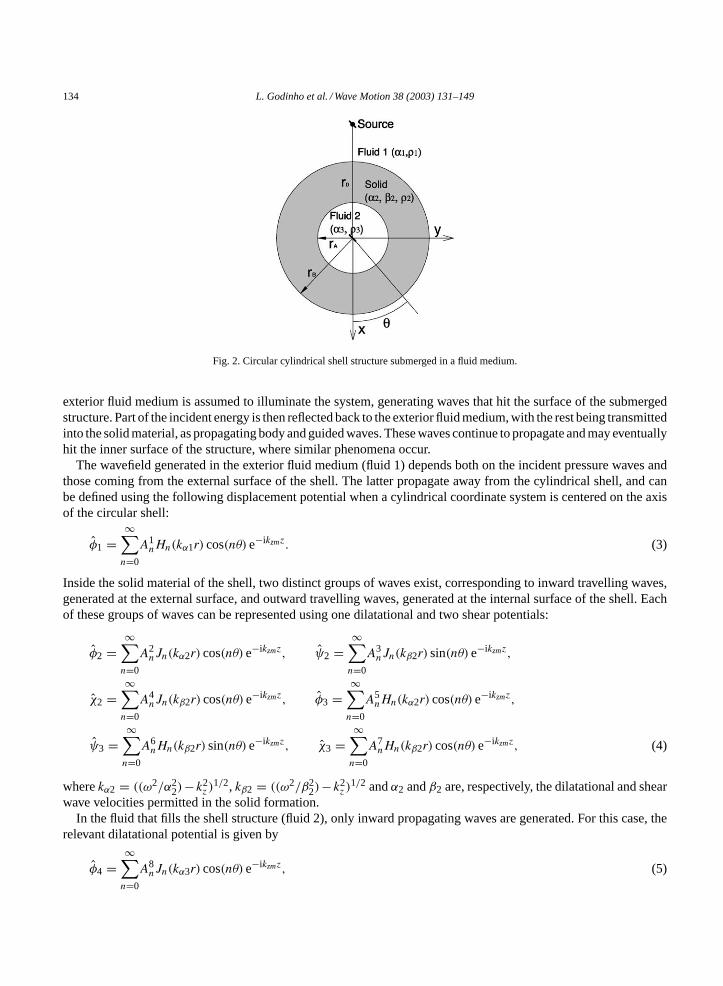
Consider a circular shell solid structure, defined by the internal and external radiirA andrB, respectively, andsubmerged in a homogenous fluid medium, as illustrated inFig. 2. A harmonic dilatational source placed in the


Fig. 2. Circular cylindrical shell structure submerged in a fluid medium.

exterior fluid medium is assumed to illuminate the system, generating waves that hit the surface of the submergedstructure. Part of the incident energy is then reflected back to the exterior fluid medium, with the rest being transmittedinto the solid material, as propagating body and guided waves. These waves continue to propagate and may eventuallyhit the inner surface of the structure, where similar phenomena occur.

The wavefield generated in the exterior fluid medium (fluid 1) depends both on the incident pressure waves andthose coming from the external surface of the shell. The latter propagate away from the cylindrical shell, and canbe defined using the following displacement potential when a cylindrical coordinate system is centered on the axisof the circular shell:

φ1 =∞∑n=0

A1nHn(kα1r) cos(nθ)e−ikzmz. (3)

Inside the solid material of the shell, two distinct groups of waves exist, corresponding to inward travelling waves,generated at the external surface, and outward travelling waves, generated at the internal surface of the shell. Eachof these groups of waves can be represented using one dilatational and two shear potentials:

φ2 =∞∑n=0

A2nJn(kα2r) cos(nθ)e−ikzmz, ψ2 =

∞∑n=0

A3nJn(kβ2r) sin(nθ)e−ikzmz,

χ2 =∞∑n=0

A4nJn(kβ2r) cos(nθ)e−ikzmz, φ3 =

∞∑n=0

A5nHn(kα2r) cos(nθ)e−ikzmz,

ψ3 =∞∑n=0

A6nHn(kβ2r) sin(nθ)e−ikzmz, χ3 =

∞∑n=0

A7nHn(kβ2r) cos(nθ)e−ikzmz, (4)

wherekα2 = ((ω2/α22)−k2

z )1/2, kβ2 = ((ω2/β2

2)−k2z )

1/2 andα2 andβ2 are, respectively, the dilatational and shearwave velocities permitted in the solid formation.

In the fluid that fills the shell structure (fluid 2), only inward propagating waves are generated. For this case, therelevant dilatational potential is given by

φ4 =∞∑n=0

A8nJn(kα3r) cos(nθ)e−ikzmz, (5)


wherekα3 = ((ω2/α23) − k2

z )1/2 andα3 is the pressure wave velocity in the inner fluid. The termsA

jn(j = 1,8)

for each potential of the expressions (3)–(5) are unknown coefficients to be determined by imposing the requiredboundary conditions. For our case, these boundary conditions are the continuity of normal displacements and stressesand null tangential stresses on the two solid–fluid interfaces.

In order to establish the appropriate equation system, the incident field must be expressed in terms of wavescentered on the axis of the circular cylindrical shell structure. This can be achieved with the aid of Graf’s additiontheorem, leading to the expression (in cylindrical coordinates):

φinc = − i

2

∞∑n=0

(−1)nεnHn(kα1r0)Jn(kα1r) cos(nθ)e−ikzmz, (6)

wherer0 is the distance from the source to the axis of the circular shell.The solution of the equation system can then be used to compute the stresses in the solid medium as a summation

of solutions obtained for pairs of values ofn andkz. The final system of equations is presented inAppendix A.

4. Boundary element formulation

The BEM only requires the discretization of the internal and external boundaries of the shell. Detailed informationon the BEM formulation applicable to the present problem can be found in Beskos[11].

The system of equations required for the solution is arranged so as to impose the continuity of the normaldisplacements, and normal stresses and null shear stresses along each interface between the fluid media and theshell structure. This system of equations requires the evaluation of the following integrals along the appropriatelydiscretized boundaries:

H(s)klij =

∫Cl

H(s)ij (xk, xl, nl)dCl (i, j = 1,2,3), H

(f )klf1 =

∫Cl

H(f )f1(xk, xl, nl)dCl,

G(s)klij =

∫Cl

G(s)ij (xk, xl)dCl (i = 1,2,3; j = 1), G

(f )klf1 =

∫Cl

G(f )f1(xk, xl)dCl (7)

in whichH(s)ij (xk, xl, nl) andG(s)

ij (xk, xl) are the Green’s tensor for traction and displacement components, respec-tively, in the elastic medium, at pointxl, in directionj, caused by a concentrated load acting at the source pointxk

in directioni; H(f )f1(xk, xl, nl) are the components of the Green’s tensor for pressure in the fluid medium, at point

xl, caused by a pressure load acting at the source pointxk; G(f )f1(xk, xl) are the components of the Green’s tensor

for displacement in the fluid medium, at pointxl, in the normal direction, caused by a pressure load acting at thesource pointxk; nl is the unit outward normal for thelth boundary segmentCl; the subscriptsi, j = 1,2,3 denotethe normal, tangential andz-directions, respectively. These equations are conveniently transformed from thex, y, z

Cartesian coordinate system by means of standard vector transformation operators. The required 2.5D fundamentalsolutions (Green’s functions) in Cartesian co-ordinates, for the elastic and fluid media, are given below:

• Elastic medium:

Gxx = A

[k2s H0β − 1

rB1 + γ2

xB2

], Gyy = A

[k2s H0β − 1

rB1 + γ2

yB2

],

Gzz = A[k2s H0β − k2

zB0], Gxy = Gyx = γxγyAB2, Gxz = Gzx = ikzγxAB1,

Gyz = Gzy = ikzγyAB1, (8)

whereλ,µare the Lamé constants;ρ the mass density;α = ((λ+2µ)/ρ)1/2 the P wave velocity;β = (µ/ρ)1/2 theS wave velocity;kp = ω/α, ks = ω/β the wave number;kα = (k2

p − k2z )

1/2, kβ = (k2s − k2

z )1/2 the wave number;


A = 1/4iρω2 the amplitude;γi = ∂r/∂xi = xi/r (i = 1,2) the direction cosines;Hnα = H(2)n (kαr),Hnβ =

H(2)n (kβr) the Hankel functions;Bn = knβHnβ − knαHnα theBn functions.

• Fluid media:

Gfx = −AfkαfH1αf γx, Gfy = −AfkαfH1αf γy, (9)

wherekαf = (k2pf − k2

z )1/2 is the wave number;Af = 1/4i the amplitude;Hnαf = H

(2)n (kαf r) the Hankel

functions.

Fig. 3. Validation of the BEM algorithm: (a) geometry of the model; (b) response computed at receiver R.


The required integrations inEq. (7)are performed analytically for the loaded element, and by using a Gaussianquadrature scheme when the element to be integrated is not the loaded element.

5. BEM validation

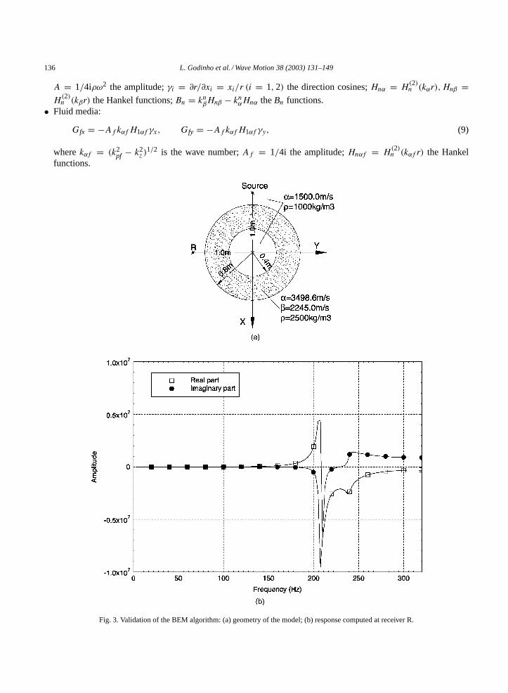
The results computed by the present BEM algorithm were compared with those obtained analytically usingthe formulation described above.Fig. 3a illustrates the geometry of the model used in the validation, assuminga cylindrical circular elastic shell structure, with an internal diameter of 0.8 m and an external diameter of 1.6 m,inserted in an infinite fluid medium. The mechanical properties of the elastic medium and those of the two fluidsare listed in the same figure.

A spatially sinusoidal harmonic pressure line load is applied atx = −1.0 m andy = 0.0 m. Computations areachieved in the frequency domain [2.50, 320.0 Hz] with a frequency increment of 2.5 Hz.

Fig. 3b displays the real and imaginary parts of the scattered pressure field recorded by the receiver placed atx = 0.0 m andy = −1.0 m (labeled R), for a pressure line load withkz = 1.0 rad/m. The solid lines represent theanalytical solutions, while the marked line corresponds to the BEM solution. The square marks indicate the realpart of the response, while the round marks refer to the imaginary part.

The results computed at receiver R enable one to conclude that the two solutions are in very close agreement,indicating that the BEM model is accurate. Equally good results were achieved from tests in which different loadsand receivers were situated at different points.

6. Time responses

After obtaining frequency domain responses, the pressure in the spatial–temporal domain is computed by anumerical fast inverse Fourier transform inω. For this purpose, the pressure point source is assumed to have atemporal variation defined by a Ricker pulse. In the frequency domain, this pulse is defined as

U(ω) = A[2√πt0 e−iωts

]Ω2 e−Ω2

(10)

in whichΩ = ωt0/2, t denotes time andπt0 the characteristic (dominant) period of the wavelet.This technique allows analyses for a total time window ofT = 2π/-ω, where-ω is the frequency step. Pulses

arriving at times later thanT will appear again in the beginning of this window, generating the so-called aliasingphenomenon. To avoid the contribution of these pulses, complex frequencies of the formωc = ω − iη (withη = 0.7-ω) are used (e.g.[12]). In the time domain, this shift is taken into account by applying an exponentialwindow eηt to the response[13].

7. Numerical examples

All the examples given here have a cylindrical shell structure defined by two circular cylindrical surfaces. Theinner surface has a diameter of 1.00 m while that of the outer surface is 1.40 m. Each surface is modeled using150 boundary elements. This structure is submerged in a fluid medium, which allows a pressure wave propagationvelocity of 1500 m/s and exhibits a density ofρ = 1000 kg/m3. The fluid filling the shell is assumed to have thesame properties as the host medium, while the elastic material of the shell structure is concrete, with a Poisson ratioof ν = 0.15, a density ofρ = 2500 kg/m3 and Young’s modulusE = 29.0 GPa, allowing propagation velocities forthe P and S waves of 3498.6 and 2245.0 m/s, respectively. Pressure responses are calculated at four sets of receiversplaced in the fluid filling the structure. Each set consists of a line of five receivers, placed along thez-direction andwith differentz-coordinates. Thez-coordinate of each receiver is indicated in the time responses.


Fig. 4. Geometry of the model: (a) case 1; (b) case 2.

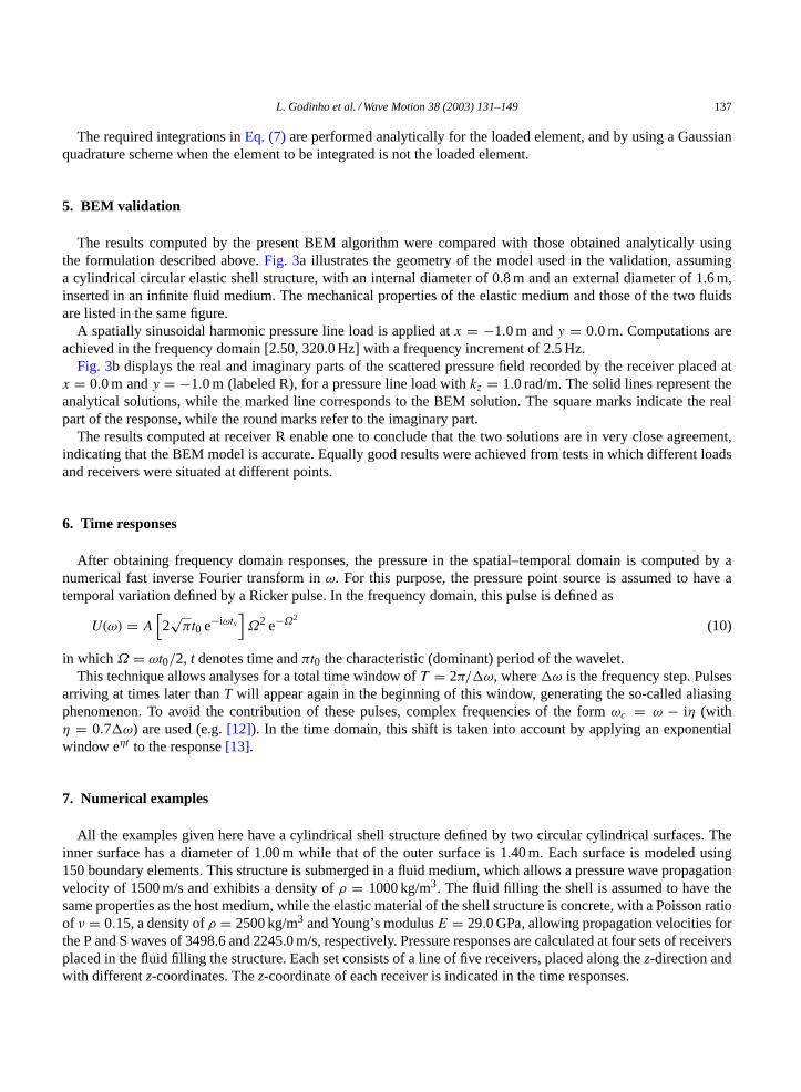
Two distinct situations are simulated, as shown inFig. 4. The first corresponds to a cylindrical shell structuredefined by two concentric circumferences, with a constant wall thickness of 0.20 m (case 1,Fig. 4a). In the secondsituation, the cylindrical shell structure is assumed to have a construction defect; thus, two non-concentric circum-ferences define the structure, with their centers placed 0.05 m apart (case 2,Fig. 4b). For both cases, point pressureloads, placed either inside (position O1) or outside (position O2) the structure, illuminate the dynamic system. The3D response is given by a discrete summation of 2.5D responses, as described inSection 2.

All the computations were performed for frequencies in the range of 8–1024 Hz, with increments of 8 Hz. Thisfrequency step determines a maximum time analysis of 0.125 ms for the time domain responses. The time domainresponses presented are computed by means of an inverse Fourier transformation, assuming the source generates aRicker pulse with a central frequency of 350.0 Hz.

7.1. Case 1—cylindrical shell structure with cross-section defined by two concentric circumferences

Fig. 5a displays both the frequency vs. phase velocity and the time domain pressures responses computed atreceivers R1, when a point pressure load is excited at position O1, within the case 1 structure. The response in thefrequency vs. phase velocity domain is determined by computing the solution of the problem for different valuesof the parameterkz = ω/c, with c being the apparent wave velocity alongz. For these figures to be understoodmore easily, the frequency vs. phase velocity responses only represent phase velocities ranging from 800.0 to1600.0 m/s. The response registered for higher phase velocities is omitted in these figures. However, time responsesare calculated for the full range of velocities, and thus they take into account the contribution of all waves involved.

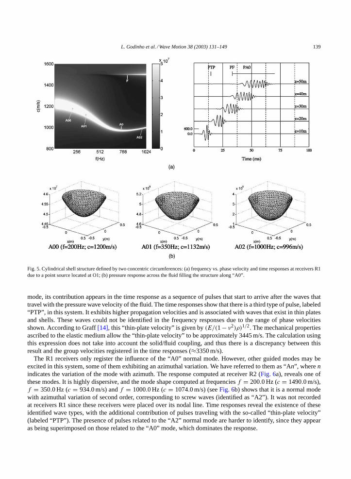
The response registered at receivers R1 (Fig. 5a), placed over the geometric center of the system, reveals theexistence of different types of waves. In the frequency vs. phase velocity response, waves traveling in the fluidwith the pressure wave propagation velocity of 1500.0 m/s are clearly visible (labeled “F”). An additional excitedmode can also be seen (labeled as “A0”). This mode corresponds to dispersive guided waves, exhibiting phasevelocities below the fluid pressure wave velocity. It seems to exist in the full frequency range. Its mode shape wascomputed over a fine grid of receivers placed inside the structure, for frequencies off = 200.0 Hz (c = 1200.0 m/s),f = 350.0 Hz (c = 1132.0 m/s) andf = 1000.0 Hz (c = 996.0 m/s), illustrated inFig. 5b. In Fig. 5a, a pair ofnumbers identifies the frequency position of each of these points (Aij ), the first number identifying the azimuthalorder of the mode and the second giving its relative position in the frequency domain. For this case, it clearlyindicates that this is an axisymmetric mode and its shape remains constant with the frequency variation.

The features described can also be identified in the time domain responses ofFig. 5a. A pulse can be detectedin the time responses, corresponding to waves traveling with the fluid velocity, and labeled as “PF”. There followsa dense ring of pulses associated with the “A0” normal mode (labeled “PA0”). Since “A0” is a highly dispersive


Fig. 5. Cylindrical shell structure defined by two concentric circumferences: (a) frequency vs. phase velocity and time responses at receivers R1due to a point source located at O1; (b) pressure response across the fluid filling the structure along “A0”.

mode, its contribution appears in the time response as a sequence of pulses that start to arrive after the waves thattravel with the pressure wave velocity of the fluid. The time responses show that there is a third type of pulse, labeled“PTP”, in this system. It exhibits higher propagation velocities and is associated with waves that exist in thin platesand shells. These waves could not be identified in the frequency responses due to the range of phase velocitiesshown. According to Graff[14], this “thin-plate velocity” is given by(E/(1− ν2)ρ)1/2. The mechanical propertiesascribed to the elastic medium allow the “thin-plate velocity” to be approximately 3445 m/s. The calculation usingthis expression does not take into account the solid/fluid coupling, and thus there is a discrepancy between thisresult and the group velocities registered in the time responses (≈3350 m/s).

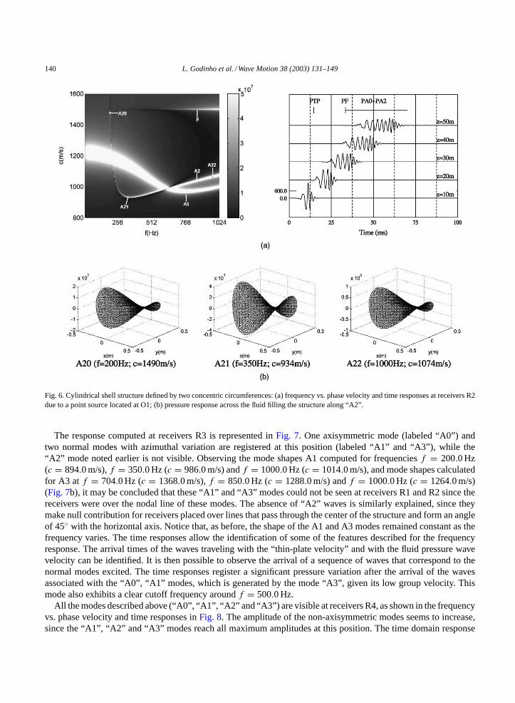
The R1 receivers only register the influence of the “A0” normal mode. However, other guided modes may beexcited in this system, some of them exhibiting an azimuthal variation. We have referred to them as “An”, wherenindicates the variation of the mode with azimuth. The response computed at receiver R2 (Fig. 6a), reveals one ofthese modes. It is highly dispersive, and the mode shape computed at frequenciesf = 200.0 Hz (c = 1490.0 m/s),f = 350.0 Hz (c = 934.0 m/s) andf = 1000.0 Hz (c = 1074.0 m/s) (seeFig. 6b) shows that it is a normal modewith azimuthal variation of second order, corresponding to screw waves (identified as “A2”). It was not recordedat receivers R1 since these receivers were placed over its nodal line. Time responses reveal the existence of theseidentified wave types, with the additional contribution of pulses traveling with the so-called “thin-plate velocity”(labeled “PTP”). The presence of pulses related to the “A2” normal mode are harder to identify, since they appearas being superimposed on those related to the “A0” mode, which dominates the response.


Fig. 6. Cylindrical shell structure defined by two concentric circumferences: (a) frequency vs. phase velocity and time responses at receivers R2due to a point source located at O1; (b) pressure response across the fluid filling the structure along “A2”.

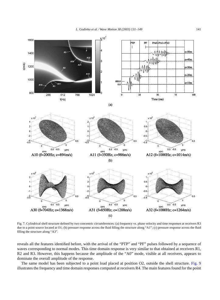
The response computed at receivers R3 is represented inFig. 7. One axisymmetric mode (labeled “A0”) andtwo normal modes with azimuthal variation are registered at this position (labeled “A1” and “A3”), while the“A2” mode noted earlier is not visible. Observing the mode shapes A1 computed for frequenciesf = 200.0 Hz(c = 894.0 m/s),f = 350.0 Hz (c = 986.0 m/s) andf = 1000.0 Hz (c = 1014.0 m/s), and mode shapes calculatedfor A3 atf = 704.0 Hz (c = 1368.0 m/s),f = 850.0 Hz (c = 1288.0 m/s) andf = 1000.0 Hz (c = 1264.0 m/s)(Fig. 7b), it may be concluded that these “A1” and “A3” modes could not be seen at receivers R1 and R2 since thereceivers were over the nodal line of these modes. The absence of “A2” waves is similarly explained, since theymake null contribution for receivers placed over lines that pass through the center of the structure and form an angleof 45 with the horizontal axis. Notice that, as before, the shape of the A1 and A3 modes remained constant as thefrequency varies. The time responses allow the identification of some of the features described for the frequencyresponse. The arrival times of the waves traveling with the “thin-plate velocity” and with the fluid pressure wavevelocity can be identified. It is then possible to observe the arrival of a sequence of waves that correspond to thenormal modes excited. The time responses register a significant pressure variation after the arrival of the wavesassociated with the “A0”, “A1” modes, which is generated by the mode “A3”, given its low group velocity. Thismode also exhibits a clear cutoff frequency aroundf = 500.0 Hz.

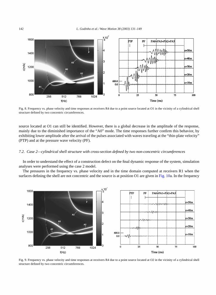
All the modes described above (“A0”, “A1”, “A2” and “A3”) are visible at receivers R4, as shown in the frequencyvs. phase velocity and time responses inFig. 8. The amplitude of the non-axisymmetric modes seems to increase,since the “A1”, “A2” and “A3” modes reach all maximum amplitudes at this position. The time domain response


Fig. 7. Cylindrical shell structure defined by two concentric circumferences: (a) frequency vs. phase velocity and time responses at receivers R3due to a point source located at O1; (b) pressure response across the fluid filling the structure along “A1”; (c) pressure response across the fluidfilling the structure along “A3”.

reveals all the features identified before, with the arrival of the “PTP” and “PF” pulses followed by a sequence ofwaves corresponding to normal modes. This time domain response is very similar to that obtained at receivers R1,R2 and R3. However, this happens because the amplitude of the “A0” mode, visible at all receivers, appears todominate the overall amplitude of the response.

The same model has been subjected to a point load placed at position O2, outside the shell structure.Fig. 9illustrates the frequency and time domain responses computed at receivers R4. The main features found for the point


Fig. 8. Frequency vs. phase velocity and time responses at receivers R4 due to a point source located at O1 in the vicinity of a cylindrical shellstructure defined by two concentric circumferences.

source located at O1 can still be identified. However, there is a global decrease in the amplitude of the response,mainly due to the diminished importance of the “A0” mode. The time responses further confirm this behavior, byexhibiting lower amplitude after the arrival of the pulses associated with waves traveling at the “thin-plate velocity”(PTP) and at the pressure wave velocity (PF).

7.2. Case 2—cylindrical shell structure with cross-section defined by two non-concentric circumferences

In order to understand the effect of a construction defect on the final dynamic response of the system, simulationanalyses were performed using the case 2 model.

The pressures in the frequency vs. phase velocity and in the time domain computed at receivers R1 when thesurfaces defining the shell are not concentric and the source is at position O1 are given inFig. 10a. In the frequency

Fig. 9. Frequency vs. phase velocity and time responses at receivers R4 due to a point source located at O2 in the vicinity of a cylindrical shellstructure defined by two concentric circumferences.


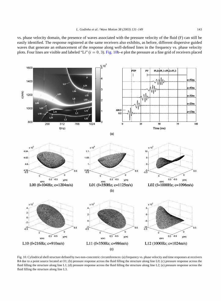
vs. phase velocity domain, the presence of waves associated with the pressure velocity of the fluid (F) can still beeasily identified. The response registered at the same receivers also exhibits, as before, different dispersive guidedwaves that generate an enhancement of the response along well-defined lines in the frequency vs. phase velocityplots. Four lines are visible and labeled “Li” ( i = 0,3).Fig. 10b–e plot the pressure at a fine grid of receivers placed

Fig. 10. Cylindrical shell structure defined by two non-concentric circumferences: (a) frequency vs. phase velocity and time responses at receiversR4 due to a point source located at O1; (b) pressure response across the fluid filling the structure along line L0; (c) pressure response across thefluid filling the structure along line L1; (d) pressure response across the fluid filling the structure along line L2; (e) pressure response across thefluid filling the structure along line L3.


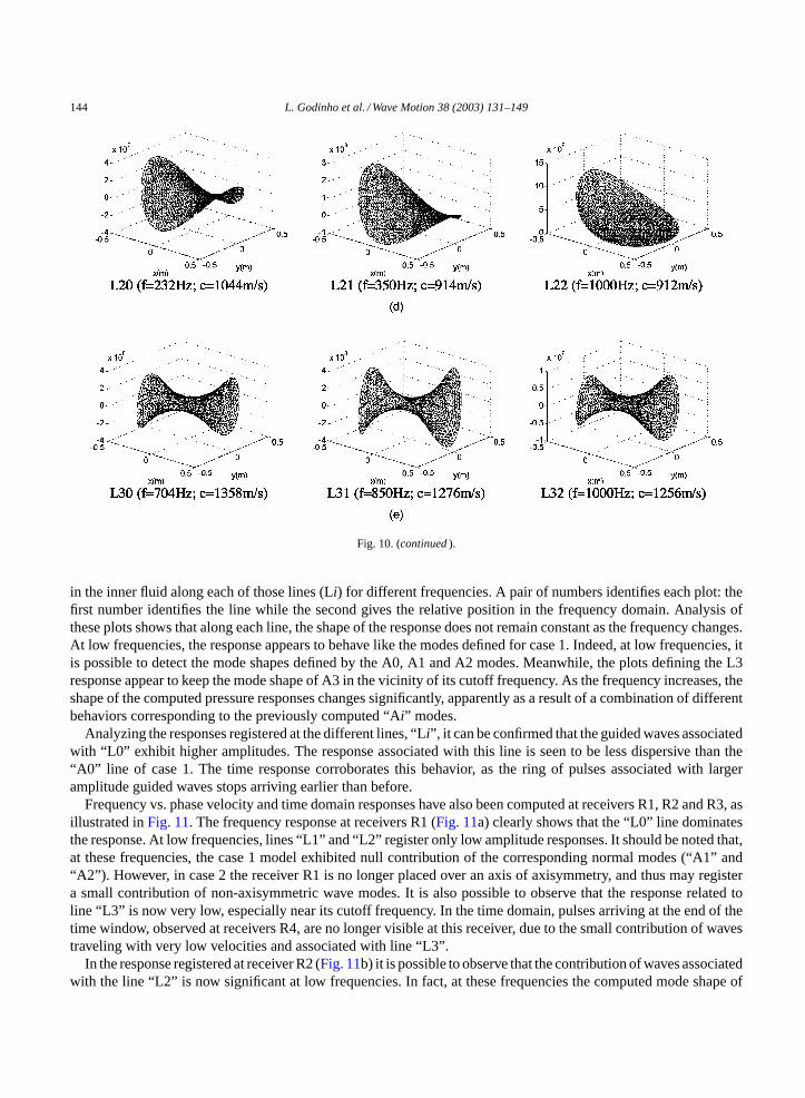
Fig. 10. (continued).

in the inner fluid along each of those lines (Li) for different frequencies. A pair of numbers identifies each plot: thefirst number identifies the line while the second gives the relative position in the frequency domain. Analysis ofthese plots shows that along each line, the shape of the response does not remain constant as the frequency changes.At low frequencies, the response appears to behave like the modes defined for case 1. Indeed, at low frequencies, itis possible to detect the mode shapes defined by the A0, A1 and A2 modes. Meanwhile, the plots defining the L3response appear to keep the mode shape of A3 in the vicinity of its cutoff frequency. As the frequency increases, theshape of the computed pressure responses changes significantly, apparently as a result of a combination of differentbehaviors corresponding to the previously computed “Ai” modes.

Analyzing the responses registered at the different lines, “Li”, it can be confirmed that the guided waves associatedwith “L0” exhibit higher amplitudes. The response associated with this line is seen to be less dispersive than the“A0” line of case 1. The time response corroborates this behavior, as the ring of pulses associated with largeramplitude guided waves stops arriving earlier than before.

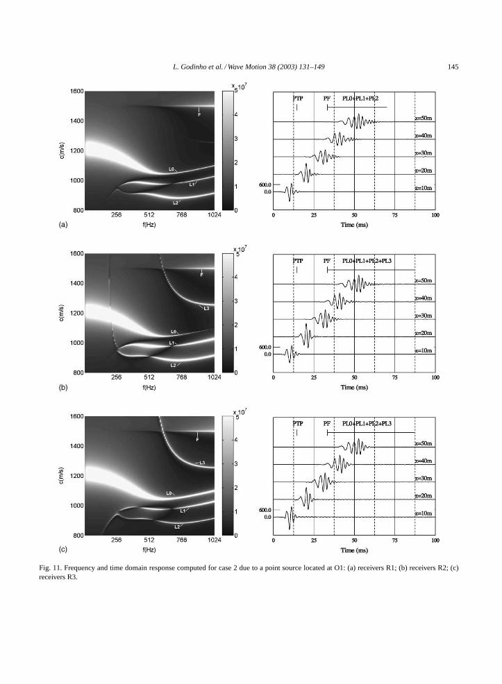
Frequency vs. phase velocity and time domain responses have also been computed at receivers R1, R2 and R3, asillustrated inFig. 11. The frequency response at receivers R1 (Fig. 11a) clearly shows that the “L0” line dominatesthe response. At low frequencies, lines “L1” and “L2” register only low amplitude responses. It should be noted that,at these frequencies, the case 1 model exhibited null contribution of the corresponding normal modes (“A1” and“A2”). However, in case 2 the receiver R1 is no longer placed over an axis of axisymmetry, and thus may registera small contribution of non-axisymmetric wave modes. It is also possible to observe that the response related toline “L3” is now very low, especially near its cutoff frequency. In the time domain, pulses arriving at the end of thetime window, observed at receivers R4, are no longer visible at this receiver, due to the small contribution of wavestraveling with very low velocities and associated with line “L3”.

In the response registered at receiver R2 (Fig. 11b) it is possible to observe that the contribution of waves associatedwith the line “L2” is now significant at low frequencies. In fact, at these frequencies the computed mode shape of


Fig. 11. Frequency and time domain response computed for case 2 due to a point source located at O1: (a) receivers R1; (b) receivers R2; (c)receivers R3.


“L2” is very similar to the “A2” mode of case 1, reaching maximum amplitude at this receiver. Furthermore, thecontribution of waves associated with the response line “L3” is now more evident, in particular at frequencies closerto the cutoff frequency of this line. The time response is very similar to that observed at R1, with pulses arriving atlater times, associated with the “L3” line having a slight amplitude increase.

At receivers R3 (Fig. 11c), it can be seen that the line “L2” shows very low amplitudes at low frequencies, whilethe importance of the “L1” line seems to increase. Again, this behavior was expected, since for low frequenciesthese lines approach the case 1 mode shape of the “A2” and “A1” modes, respectively. The amplitude of the “L3”response line is also greatly enhanced at this receiver. The time response further confirms this behavior, with pulsesarriving at later times appearing with higher amplitudes.

Simulations were also performed for the same model, assuming the excitation source to be placed at positionO2 (not shown). As in case 1, the main features described when the point source was located at O1 can still beidentified. Both frequency and time responses reveal a global fall in amplitude, which is even more evident than incase 1. In the time domain, the pulses associated with waves traveling with the “thin-plate velocity” (PTP), with thepressure wave velocity (PF) and with the normal modes excited (Li) can be identified.

8. Conclusions

The pressure inside an infinite cylindrical shell structure, submerged in a homogeneous fluid medium, andsubjected to the incidence of waves generated by a point pressure load, has been computed. The structure wasmodeled as an elastic material, and the full interaction between the two fluids and the structure was taken intoaccount. Two different models were analyzed, corresponding to shell structures defined by two concentric ornon-concentric circumferences. Results were obtained in both the frequency and time domains, allowing the mainfeatures of the wave propagation to be identified.

The results obtained when the inner and outer surfaces are defined by two concentric circumferences reveal thatmultiple normal modes are excited and their contribution to the response depends on the position of the receiver. Thedifferent normal modes excited were clearly identified and their mode shape was computed, revealing a constantbehavior with the frequency variation.

When the structure is defined by non-concentric circular surfaces, the pressure response in the frequency vs. phasevelocity domain allowed the identification of well defined lines where the response exhibits higher amplitudes. Atlow frequencies and near the cutoff frequencies of these lines, the behavior of the response seems to approachthat of the normal modes identified when the circumferences defining the inner and outer surfaces of the shell areconcentric. However, as the frequency increases, the mode shapes computed indicate that the pressure responseresults from a combination of the different types of guided waves generated when the structure is defined by twoconcentric circumferences. This can be seen in both the frequency and time domains, and for the different receiversand source positions analyzed.

Appendix A

The eight potentials defined before allow the definition of a system of eight equations for eight unknowns, toyield the coefficientsAi

n (i = 1, . . . ,8). The equation system is built so as to allow the establishment of boundaryconditions of null tangential stresses and the continuity of normal displacements and stresses in the solid–fluidinterfaces:

a11 . . . a18...

...

a81 . . . a88

A1n

...

A8n

=

b1...

b8

.


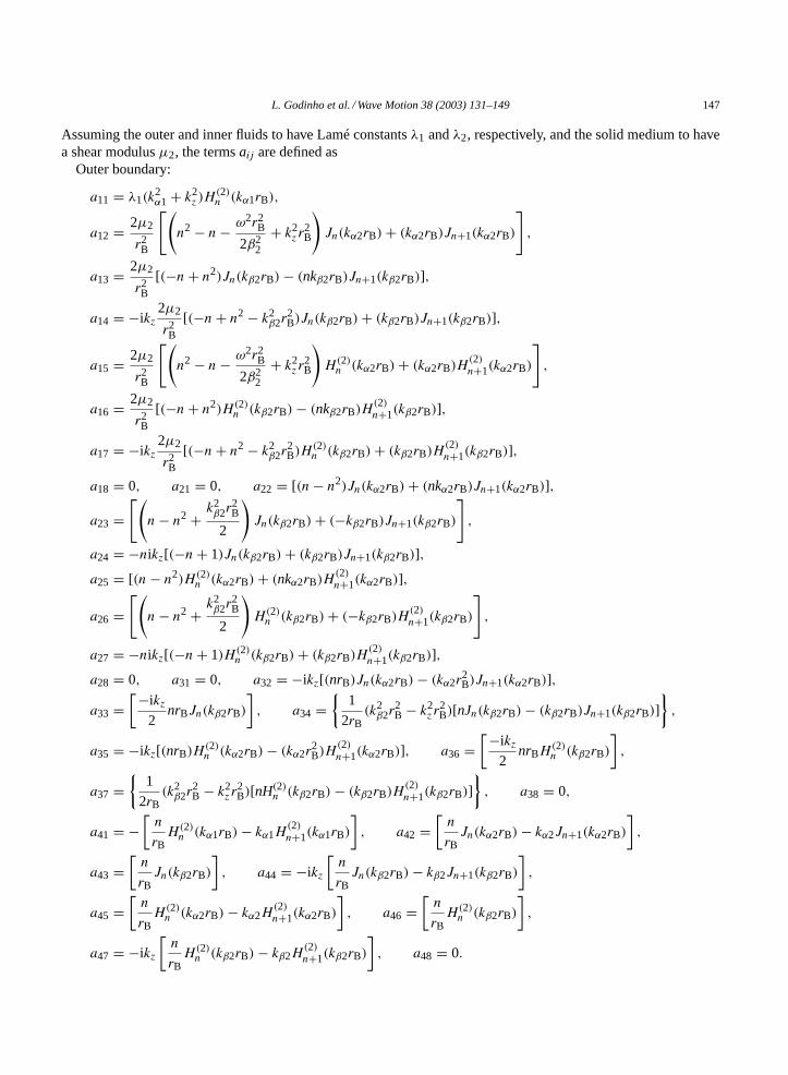
Assuming the outer and inner fluids to have Lamé constantsλ1 andλ2, respectively, and the solid medium to havea shear modulusµ2, the termsaij are defined as

Outer boundary:

a11 = λ1(k2α1 + k2

z )H(2)n (kα1rB),

a12 = 2µ2

r2B

[(n2 − n − ω2r2

B

2β22

+ k2z r

2B

)Jn(kα2rB) + (kα2rB)Jn+1(kα2rB)

],

a13 = 2µ2

r2B

[(−n + n2)Jn(kβ2rB) − (nkβ2rB)Jn+1(kβ2rB)],

a14 = −ikz2µ2

r2B

[(−n + n2 − k2β2r

2B)Jn(kβ2rB) + (kβ2rB)Jn+1(kβ2rB)],

a15 = 2µ2

r2B

[(n2 − n − ω2r2

B

2β22

+ k2z r

2B

)H(2)n (kα2rB) + (kα2rB)H

(2)n+1(kα2rB)

],

a16 = 2µ2

r2B

[(−n + n2)H(2)n (kβ2rB) − (nkβ2rB)H

(2)n+1(kβ2rB)],

a17 = −ikz2µ2

r2B

[(−n + n2 − k2β2r

2B)H

(2)n (kβ2rB) + (kβ2rB)H

(2)n+1(kβ2rB)],

a18 = 0, a21 = 0, a22 = [(n − n2)Jn(kα2rB) + (nkα2rB)Jn+1(kα2rB)],

a23 =[(

n − n2 +k2β2r

2B

2

)Jn(kβ2rB) + (−kβ2rB)Jn+1(kβ2rB)

],

a24 = −nikz[(−n + 1)Jn(kβ2rB) + (kβ2rB)Jn+1(kβ2rB)],

a25 = [(n − n2)H(2)n (kα2rB) + (nkα2rB)H

(2)n+1(kα2rB)],

a26 =[(

n − n2 +k2β2r

2B

2

)H(2)n (kβ2rB) + (−kβ2rB)H

(2)n+1(kβ2rB)

],

a27 = −nikz[(−n + 1)H(2)n (kβ2rB) + (kβ2rB)H

(2)n+1(kβ2rB)],

a28 = 0, a31 = 0, a32 = −ikz[(nrB)Jn(kα2rB) − (kα2r2B)Jn+1(kα2rB)],

a33 =[−ikz

2nrBJn(kβ2rB)

], a34 =

1

2rB(k2

β2r2B − k2

z r2B)[nJn(kβ2rB) − (kβ2rB)Jn+1(kβ2rB)]

,

a35 = −ikz[(nrB)H(2)n (kα2rB) − (kα2r

2B)H

(2)n+1(kα2rB)], a36 =

[−ikz2

nrBH(2)n (kβ2rB)

],

a37 =

1

2rB(k2

β2r2B − k2

z r2B)[nH(2)

n (kβ2rB) − (kβ2rB)H(2)n+1(kβ2rB)]

, a38 = 0,

a41 = −[n

rBH(2)n (kα1rB) − kα1H

(2)n+1(kα1rB)

], a42 =

[n

rBJn(kα2rB) − kα2Jn+1(kα2rB)

],

a43 =[n

rBJn(kβ2rB)

], a44 = −ikz

[n

rBJn(kβ2rB) − kβ2Jn+1(kβ2rB)

],

a45 =[n

rBH(2)n (kα2rB) − kα2H

(2)n+1(kα2rB)

], a46 =

[n

rBH(2)n (kβ2rB)

],

a47 = −ikz

[n

rBH(2)n (kβ2rB) − kβ2H

(2)n+1(kβ2rB)

], a48 = 0.


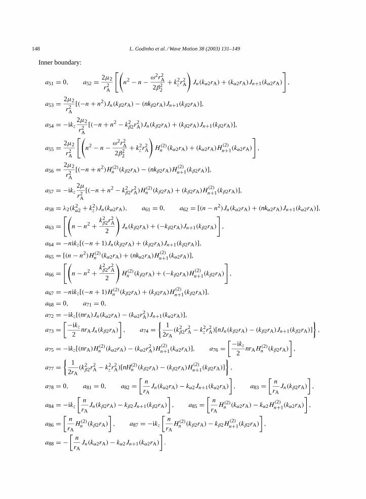
Inner boundary:

a51 = 0, a52 = 2µ2

r2A

[(n2 − n − ω2r2

A

2β22

+ k2z r

2A

)Jn(kα2rA) + (kα2rA)Jn+1(kα2rA)

],

a53 = 2µ2

r2A

[(−n + n2)Jn(kβ2rA) − (nkβ2rA)Jn+1(kβ2rA)],

a54 = −ikz2µ2

r2A

[(−n + n2 − k2β2r

2A)Jn(kβ2rA) + (kβ2rA)Jn+1(kβ2rA)],

a55 = 2µ2

r2A

[(n2 − n − ω2r2

A

2β22

+ k2z r

2A

)H(2)n (kα2rA) + (kα2rA)H

(2)n+1(kα2rA)

],

a56 = 2µ2

r2A

[(−n + n2)H(2)n (kβ2rA) − (nkβ2rA)H

(2)n+1(kβ2rA)],

a57 = −ikz2µ

r2A

[(−n + n2 − k2β2r

2A)H

(2)n (kβ2rA) + (kβ2rA)H

(2)n+1(kβ2rA)],

a58 = λ2(k2α2 + k2

z )Jn(kα2rA), a61 = 0, a62 = [(n − n2)Jn(kα2rA) + (nkα2rA)Jn+1(kα2rA)],

a63 =[(

n − n2 +k2β2r

2A

2

)Jn(kβ2rA) + (−kβ2rA)Jn+1(kβ2rA)

],

a64 = −nikz[(−n + 1)Jn(kβ2rA) + (kβ2rA)Jn+1(kβ2rA)],

a65 = [(n − n2)H(2)n (kα2rA) + (nkα2rA)H

(2)n+1(kα2rA)],

a66 =[(

n − n2 +k2β2r

2A

2

)H(2)n (kβ2rA) + (−kβ2rA)H

(2)n+1(kβ2rA)

],

a67 = −nikz[(−n + 1)H(2)n (kβ2rA) + (kβ2rA)H

(2)n+1(kβ2rA)],

a68 = 0, a71 = 0,

a72 = −ikz[(nrA)Jn(kα2rA) − (kα2r2A)Jn+1(kα2rA)],

a73 =[−ikz

2nrAJn(kβ2rA)

], a74 =

1

2rA(k2

β2r2A − k2

z r2A)[nJn(kβ2rA) − (kβ2rA)Jn+1(kβ2rA)]

,

a75 = −ikz[(nrA)H(2)n (kα2rA) − (kα2r

2A)H

(2)n+1(kα2rA)], a76 =

[−ikz2

nrAH(2)n (kβ2rA)

],

a77 =

1

2rA(k2

β2r2A − k2

z r2A)[nH(2)

n (kβ2rA) − (kβ2rA)H(2)n+1(kβ2rA)]

,

a78 = 0, a81 = 0, a82 =[n

rAJn(kα2rA) − kα2Jn+1(kα2rA)

], a83 =

[n

rAJn(kβ2rA)

],

a84 = −ikz

[n

rAJn(kβ2rA) − kβ2Jn+1(kβ2rA)

], a85 =

[n

rAH(2)n (kα2rA) − kα2H

(2)n+1(kα2rA)

],

a86 =[n

rAH(2)n (kβ2rA)

], a87 = −ikz

[n

rAH(2)n (kβ2rA) − kβ2H

(2)n+1(kβ2rA)

],

a88 = −[n

rAJn(kα2rA) − kα2Jn+1(kα2rA)

].


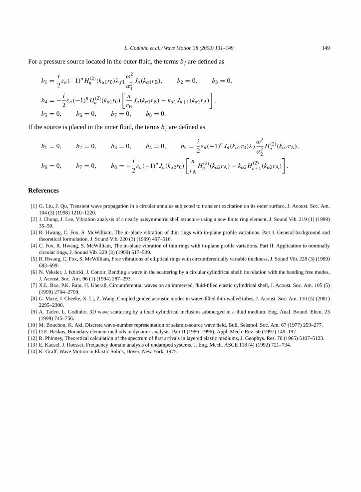
For a pressure source located in the outer fluid, the termsbj are defined as

b1 = i

2εn(−1)nH(2)

n (kα1r0)λf1ω2

α21

Jn(kα1rB), b2 = 0, b3 = 0,

b4 = − i

2εn(−1)nH(2)

n (kα1r0)

[n

rBJn(kα1rB) − kα1Jn+1(kα1rB)

],

b5 = 0, b6 = 0, b7 = 0, b8 = 0.

If the source is placed in the inner fluid, the termsbj are defined as

b1 = 0, b2 = 0, b3 = 0, b4 = 0, b5 = i

2εn(−1)nJn(kα2r0)λ2

ω2

α22

H(2)n (kα2rA),

b6 = 0, b7 = 0, b8 = − i

2εn(−1)nJn(kα2r0)

[n

rAH(2)n (kα2rA) − kα2H

(2)n+1(kα2rA)

].

References

[1] G. Liu, J. Qu, Transient wave propagation in a circular annulus subjected to transient excitation on its outer surface, J. Acoust. Soc. Am.104 (3) (1998) 1210–1220.

[2] J. Chung, J. Lee, Vibration analysis of a nearly axisymmetric shell structure using a new finite ring element, J. Sound Vib. 219 (1) (1999)35–50.

[3] R. Hwang, C. Fox, S. McWilliam, The in-plane vibration of thin rings with in-plane profile variations. Part I. General background andtheoretical formulation, J. Sound Vib. 220 (3) (1999) 497–516.

[4] C. Fox, R. Hwang, S. McWilliam, The in-plane vibration of thin rings with in-plane profile variations. Part II. Application to nominallycircular rings, J. Sound Vib. 220 (3) (1999) 517–539.

[5] R. Hwang, C. Fox, S. McWilliam, Free vibrations of elliptical rings with circumferentially variable thickness, J. Sound Vib. 228 (3) (1999)683–699.

[6] N. Veksler, J. Izbicki, J. Conoir, Bending a wave in the scattering by a circular cylindrical shell: its relation with the bending free modes,J. Acoust. Soc. Am. 96 (1) (1994) 287–293.

[7] X.L. Bao, P.K. Raju, H. Uberall, Circumferential waves on an immersed, fluid-filled elastic cylindrical shell, J. Acoust. Soc. Am. 105 (5)(1999) 2704–2709.

[8] G. Maze, J. Cheeke, X. Li, Z. Wang, Coupled guided acoustic modes in water-filled thin-walled tubes, J. Acoust. Soc. Am. 110 (5) (2001)2295–2300.

[9] A. Tadeu, L. Godinho, 3D wave scattering by a fixed cylindrical inclusion submerged in a fluid medium, Eng. Anal. Bound. Elem. 23(1999) 745–756.

[10] M. Bouchon, K. Aki, Discrete wave-number representation of seismic-source wave field, Bull. Seismol. Soc. Am. 67 (1977) 259–277.[11] D.E. Beskos, Boundary element methods in dynamic analysis, Part II (1986–1996), Appl. Mech. Rev. 50 (1997) 149–197.[12] R. Phinney, Theoretical calculation of the spectrum of first arrivals in layered elastic mediums, J. Geophys. Res. 70 (1965) 5107–5123.[13] E. Kausel, J. Roesset, Frequency domain analysis of undamped systems, J. Eng. Mech. ASCE 118 (4) (1992) 721–734.[14] K. Graff, Wave Motion in Elastic Solids, Dover, New York, 1975.

wave scattering by inﬁnite cylindrical shell structures ......wave motion 38 (2003) 131–149 wave...

Documents