San Francisco Bay Conservation and Development Commission

Wave Exposure of Corte Madera Marsh, Marin County, California—a Field Investigation Open-File Report 2011–1183 U.S. Department of the Interior U.S. Geological Survey

This page intentionally left blank.

Wave Exposure of Corte Madera Marsh, Marin County, California—a Field Investigation

By Jessica R. Lacy and Daniel J. Hoover

Open-File Report 2011–1183

U.S. Department of the Interior U.S. Geological Survey

U.S. Department of the Interior KEN SALAZAR, Secretary

U.S. Geological Survey Marcia K. McNutt, Director

U.S. Geological Survey, Reston, Virginia 2011

For product and ordering information: World Wide Web: http://www.usgs.gov/pubprod Telephone: 1-888-ASK-USGS

For more information on the USGS—the Federal source for science about the Earth, its natural and living resources, natural hazards, and the environment: World Wide Web: http://www.usgs.gov Telephone: 1-888-ASK-USGS

Suggested citation: Lacy, J.R., and Hoover, D.J., 2011, Wave exposure of Corte Madera Marsh, Marin County, California—a field investigation: US Geological Survey Open-File Report 2011-1183, 28 p. [http://pubs.usgs.gov/of/2011/1183/].

Any use of trade, product, or firm names is for descriptive purposes only and does not imply endorsement by the U.S. Government.

Although this report is in the public domain, permission must be secured from the individual copyright owners to reproduce any copyrighted material contained within this report.

iii

Contents Introduction .................................................................................................................................................................... 1 

Objectives .................................................................................................................................................................. 1 Methods ......................................................................................................................................................................... 2 

Study site ................................................................................................................................................................... 2 Field campaign ........................................................................................................................................................... 4 Wave statistics ........................................................................................................................................................... 6 Bed-sediment grain size............................................................................................................................................. 7 Time and direction conventions ................................................................................................................................. 7 

Results ......................................................................................................................................................................... 7 Conditions during deployment .................................................................................................................................... 7 Bed-sediment grain size............................................................................................................................................. 8 Tidal elevations .......................................................................................................................................................... 8 Temperature and salinity ...........................................................................................................................................11 Currents ....................................................................................................................................................................13 Waves .....................................................................................................................................................................13 Ferry wakes ..............................................................................................................................................................23 

Summary and Conclusions ...........................................................................................................................................26 Acknowledgments ........................................................................................................................................................27 References Cited ..........................................................................................................................................................27 Appendix .......................................................................................................................................................................28 

Figures 1.  San Francisco Bay region. A, location of study area and Richmond meteorological station (RCMC1). B,

Aerial photograph of marsh with M1 and M2 locations. C,1980 bathymetry and stations.. ............................... 3 2.  Approximate bed elevation along study transect .................................................................................................. 4 3.  Tripod deployment at station S2.. ........................................................................................................................ 5 4.  Tides and Delta outflow for January-March 2010. ................................................................................................ 8 5.  Meteorologic conditions at Richmond meteorological station RCMC1 January-March 2010.. ............................. 9 6.  Grain-size distribution in top 2 cm of grab samples collected at S1-S3 and DP on January 28 and

March 18, 2010…………... ............................................................................................................................. 10 7.  A, Tidal elevations measured at the three ADV stations, M1, and M2, from January 25 to February 8,

2010. B, Difference in water depth between stations M2 and M1.. ................................................................. 11 8.  Time series from January 22 to March 24, 2010 of A, depth at S2 showing tidal fluctuations, and B,

temperature and C, salinity, 1 m below the water surface and 0.5 m above the bed (mab) at DP, and 0.5 mab at S2. ................................................................................................................................................ 12 

9.  Tidal currents at 30-minute intervals from February 1 to February 6, 2010, showing variation from spring to neap tides ........................................................................................................................................ 14 

10.  Current profiles from ADCP at station DP for March 1-7, 2010. ........................................................................ 15 11.  Tidally averaged (30-hour lowpass filtered) currents at stations in Corte Madera Bay. ..................................... 16 12.  A, Speed and direction of spring-tide tidal currents at stations DP-T (depth averaged), S1, S2, and S3.

B, Speed and direction of mean tidally averaged currents at DP-T, and at S1, S2, and S3. .......................... 17 

iv

13.  Time series of wave statistics and tidal elevations from ADCP at station DP-T. A, Significant wave height. B, Peak wave period. C, Wave direction. D, Water depth, and E, Nondirectional spectra of wave energy.. ................................................................................................................................................. 18 

14.  High-frequency water depths from a burst at 0400 February 5, 2010 UTC at stations S3 (A), S2 (B), S1 (C), and M2 (D). .............................................................................................................................................. 19 

15.  Spectra of wave height (A,C) and velocity in principal direction (B,D) from two 8-minute bursts, at stations S1-S3 and M2.. ................................................................................................................................. 20 

16.  Wave statistics at all stations for 5-day period including the February 5, 2010 wave event. .............................. 21 17.  Wave statistics at all stations for 5-day period including the February 24 and 26-27, 2010 wave

events…………. .............................................................................................................................................. 22 18.  Factors influencing wave damping. A, Normalized wave height (ratio of local significant wave height Hs

to Hs at station DP) versus water depth relative to MLLW. B, Normalized wave height versus wave direction at DP. C, Normalized wave height versus Hs at DP. ........................................................................ 24 

19.  Examples of ferry wakes at low tide (A, B), mid tide (C, D) and high tide (E, F). Water depths at S3 have been offset by -0.5 m to facilitate comparison between stations. ........................................................... 25 

Tables 1.  Station locations .................................................................................................................................................. 5 2.  Instrumentation and sampling schemes ............................................................................................................... 6 3.  Bed sediment grab sample times and locations ................................................................................................... 7 

v

Conversion Factors SI to Inch/Pound

Multiply By To obtain

Length

centimeter (cm) 0.3937 inch (in.)

millimeter (mm) 0.03937 inch (in.)

micrometer (um) 0.00003937 inch (in.)

meter (m) 3.281 foot (ft)

kilometer (km) 0.6214 mile (mi)

meter (m) 1.094 yard (yd)

Flow rate

meter per second (m/s) 3.281 foot per second (ft/s)

Pressure

hectopascal (hPa) 0.0009869 atmosphere, standard (atm)

hectopascal (hPa) 1 millibar (mbar) Temperature in degrees Centigrade (°C) is converted to degrees Fahrenheit (°F) as follows: °F=(1.8×°C)+32 Vertical coordinate information is referenced to the North American Vertical Datum of 1988 (NAVD 88). Altitude, as used in this report, refers to distance above the vertical datum. Pacific Standard Time (PST) = Universal Time, Coordinated (UTC) – 8 hours.

vi

Glossary Term Definition Bottom orbital velocity (ub) Maximum near-bed wave velocity during a wave period Delta Outflow An estimate of the average daily flow of freshwater from

the Sacramento-San Joaquin Delta to San Francisco Bay. Diurnal Recurring daily Frequency Inverse of period Hertz s-1, unit of frequency Mean high water The average of all high water heights over the

national tidal datum epoch (NTDE) Mean Lower-Low Water The average of the lower low water height of each tidal day

over the NTDE Neap tides Tides with the smallest range of the lunar cycle, which occur in

the first and third quarters of the moon Peak wave period (Tp) Period of the highest waves in the sampling interval Phi (Φ) Negative of the base-2 logarithm of the grain-size diameter

in millimeters. Phi units simplify calculation of grain size statistics because distributions are typically lognormal.

Representative bottom orbital Root-mean-square value of ub during the sampling interval velocity (ubr) Significant wave height (Hs) Average height (trough to crest) of the highest third of

waves during the sampling interval Spring tides Tides with the greatest range of the lunar cycle, which occur

at the time of the new or full moon Tidally-averaged Averaged over a diurnal tidal cycle

Wave Exposure of Corte Madera Marsh, Marin County, California—a Field Investigation

By Jessica R. Lacy and Daniel J. Hoover

Introduction Tidal wetlands provide valuable habitat, are an important source of primary productivity, and

can help to protect the shoreline from erosion by attenuating approaching waves. These functions are threatened by the loss of tidal marshes, whether due to erosion, sea-level rise, or land-use practices. Erosion protection by wetlands is expected to vary geographically, because wave attenuation in marshes depends on vegetation type, density, and height (Moller, 2006) and wave attenuation over mudflats depends on slope and sediment properties (Le Hir and others, 2000). In macrotidal northern European marshes, a 50 percent reduction in wave height within tens of meters of vegetated salt marsh has been observed (Moller, 1999; 2006). This study was designed to evaluate the role of mudflats and marshes in attenuating waves at a site in San Francisco Bay.

In prehistoric times, the shoreline of San Francisco Bay was ringed with tidal wetlands, with mudflats at lower elevations and marshes above. Most of the marshes around the Bay emerged 2,000-4,000 years ago, after the rate of sea-level rise slowed to approximately 1 mm/year (Atwater, 1979). Approximately 80 percent of the acreage of tidal marsh and 40 percent of the acreage of tidal mudflats in San Francisco Bay have been lost to filling and draining since 1800 (Monroe and others, 1999). Tidal wetlands are particularly susceptible to impacts from sea-level rise because the vegetation at each elevation is adapted to a specific tidal-inundation regime. The maintenance of suitable marsh-plain elevations depends on a supply of sediment that can keep up with the rate of sea-level rise (Atwater, 1979). Sea-level rise, which according to recent projections may reach 75 to 190 cm by the year 2100 (Vermeer and Rahmstorf, 2009), poses a significant threat to wetlands in San Francisco Bay, where landward migration is frequently impossible due to urbanization of the adjacent landscape.

In this study, we collected data in Corte Madera Bay and Marsh (fig. 1) to determine whether, and to what degree, waves are attenuated as they transit the Bay and, during high tides, the marsh. Corte Madera Bay was selected as a study site because of its exposure to wind waves, as well as its history of shoreline erosion and marsh restoration and monitoring. Data were collected in the winter of 2010, along a cross-shore transect extending from offshore of the subtidal mudflats into the tidal marsh. This study forms part of the Innovative Wetland Adaptation in the Lower Corte Madera Creek Watershed Project initiated by the Bay Conservation and Development Commission (BCDC) (http://www.bcdc.ca.gov/planning/climate_change/WetlandAdapt.shtml).

Objectives This study was designed to address the following questions: What are the characteristics of waves and currents in the study area, and how do they vary over time? Do wave heights or orbital velocities decrease, or wave periods change, as waves pass over the mudflats? Do wave heights decrease, or wave periods change, as waves pass over the marsh?

2

Methods

Study site Corte Madera Bay and Marsh are both in Marin County, California on the west side of Central

San Francisco Bay. The embayment is north of the Tiburon peninsula and south of the Richmond Bridge (fig. 1). Water depths throughout the embayment are less than 2 m relative to mean lower low water (MLLW), whereas depths in the adjacent main channel exceed 10 m MLLW. The Larkspur ferry landing is in the northwest corner of Corte Madera Bay, and ferries traverse Corte Madera Bay regularly through a dredged channel that runs along the north edge of the Bay (fig. 1).

Central Bay waters are strongly influenced by the Pacific Ocean, with salinities typically greater than 20 practical salinity units (psu), except during periods of high freshwater inflow through the Sacramento-San Joaquin Delta in winter. Salinities in the shallow embayments of Central Bay may be influenced by local watersheds as well: specifically, Corte Madera Creek flows into the northwest corner of Corte Madera Bay. Currents in San Francisco Bay are predominantly driven by tides at the Golden Gate. In channels, tidal currents exceed 1 m/s and are oriented along channel, whereas in shallow areas currents are weaker and their direction varies more, under the influence of local bathymetry (Walters and others, 1985).

In San Francisco Bay, winds and associated waves vary seasonally (Conomos and others, 1985). In summer, the daily sea breeze generates westerly afternoon winds as strong as 8 m/s. During winter, storms out of the south generate strong winds that can last several days and generate waves with periods as long as 5 s in areas with long fetch. Conditions are typically calm between winter storms. Corte Madera Marsh consists of three sections: an historical marsh at the north end, adjacent to the mouth of Corte Madera Creek; and two formerly diked areas that were restored to tidal action in 1976. The southern restored area, which forms the landward edge of the transect for this study, is called Muzzi Marsh. In the restored marsh the outboard levee was left partly intact for wave protection. The evolution of Muzzi Marsh has been studied extensively since the restoration (Philip Williams & Associates, Ltd. and Faber, 2004). Inner and outer Muzzi Marsh initially formed two distinct elevation zones. Inner Muzzi Marsh was filled with dredge disposal to an elevation of 2.1 m above MLLW, which is above mean higher high water. The elevation of outer Muzzi Marsh ranged from 1.1 m to 1.4 m MLLW, below the mean high water (MHW) elevation of 1.58 m MLLW. Tidal channels and a vegetated marsh plain developed in this part of the marsh, which is regularly inundated by tides. The landwardmost station in our study was located in outer Muzzi Marsh (fig. 1B).

The shoreline of Corte Madera Marsh is exposed to easterly to southeasterly wind-waves as well as wakes from the Larkspur ferry. As a result, the remaining outboard levee and adjacent marsh have progressively eroded over the past 25 years (Philip Williams & Associates, Ltd. and Faber, 2004). It should be noted that wave attenuation over marshes does not necessarily protect the marsh edge: evidence suggests that vegetation does not reduce wave-driven lateral erosion, which is the primary erosive mechanism at the marsh edge (Feagin and others, 2009). The marsh plain continues to provide a dissipative buffer between waves at the shoreline and the flood-control levee located at the west edge of the marsh.

3

Figure 1. San Francisco Bay region. A, location of study area and Richmond meteorological station (RCMC1). B, Aerial photograph of marsh with M1 and M2 locations. C,1980 bathymetry and stations. Shoreline (black outline, fig. 1C) is shown at the mean high water elevation, which is 158 cm above mean lower low water in the study area.

4

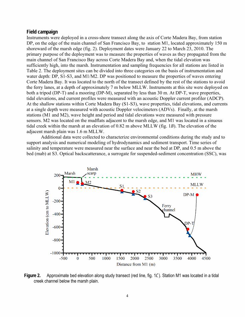
Field campaign Instruments were deployed in a cross-shore transect along the axis of Corte Madera Bay, from station DP, on the edge of the main channel of San Francisco Bay, to station M1, located approximately 150 m shoreward of the marsh edge (fig. 2). Deployment dates were January 22 to March 23, 2010. The primary purpose of the deployment was to measure the properties of waves as they propagated from the main channel of San Francisco Bay across Corte Madera Bay and, when the tidal elevation was sufficiently high, into the marsh. Instrumentation and sampling frequencies for all stations are listed in Table 2. The deployment sites can be divided into three categories on the basis of instrumentation and water depth: DP, S1-S3, and M1/M2. DP was positioned to measure the properties of waves entering Corte Madera Bay. It was located to the north of the transect defined by the rest of the stations to avoid the ferry lanes, at a depth of approximately 7 m below MLLW. Instruments at this site were deployed on both a tripod (DP-T) and a mooring (DP-M), separated by less than 30 m. At DP-T, wave properties, tidal elevations, and current profiles were measured with an acoustic Doppler current profiler (ADCP). At the shallow stations within Corte Madera Bay (S1-S3), wave properties, tidal elevations, and currents at a single depth were measured with acoustic Doppler velocimeters (ADVs). Finally, at the marsh stations (M1 and M2), wave height and period and tidal elevations were measured with pressure sensors. M2 was located on the mudflats adjacent to the marsh edge, and M1 was located in a sinuous tidal creek within the marsh at an elevation of 0.82 m above MLLW (fig. 1B). The elevation of the adjacent marsh plain was 1.6 m MLLW.

Additional data were collected to characterize environmental conditions during the study and to support analysis and numerical modeling of hydrodynamics and sediment transport. Time series of salinity and temperature were measured near the surface and near the bed at DP, and 0.5 m above the bed (mab) at S3. Optical backscatterance, a surrogate for suspended-sediment concentration (SSC), was

Figure 2. Approximate bed elevation along study transect (red line, fig. 1C). Station M1 was located in a tidal creek channel below the marsh plain.

5

measured at S1, S2, S3, and DP. Optical backscatter sensors (OBS) were equipped with mechanical wipers to minimize biofouling, and suspended-sediment samples were collected to calibrate OBS voltages to SSC. The OBS and SSC data are omitted from this report.

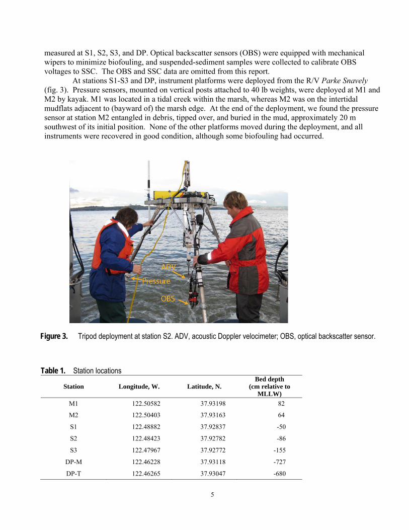
At stations S1-S3 and DP, instrument platforms were deployed from the R/V Parke Snavely (fig. 3). Pressure sensors, mounted on vertical posts attached to 40 lb weights, were deployed at M1 and M2 by kayak. M1 was located in a tidal creek within the marsh, whereas M2 was on the intertidal mudflats adjacent to (bayward of) the marsh edge. At the end of the deployment, we found the pressure sensor at station M2 entangled in debris, tipped over, and buried in the mud, approximately 20 m southwest of its initial position. None of the other platforms moved during the deployment, and all instruments were recovered in good condition, although some biofouling had occurred.

Figure 3. Tripod deployment at station S2. ADV, acoustic Doppler velocimeter; OBS, optical backscatter sensor.

Table 1. Station locations

Station Longitude, W. Latitude, N. Bed depth

(cm relative to MLLW)

M1 122.50582 37.93198 82

M2 122.50403 37.93163 64

S1 122.48882 37.92837 -50

S2 122.48423 37.92782 -86

S3 122.47967 37.92772 -155

DP-M 122.46228 37.93118 -727

DP-T 122.46265 37.93047 -680

6

Table 2. Instrumentation and sampling schemes Site Platform Instrument Parameters

measured height above

bed, m Sampling frequency

M1 Bursting pressure sensor

Tide height, wave height, and period.

0.1 Tides: 60 s average every 15 minutes. Waves: 2048 samples at 4 Hz every hour.

M2 Bursting pressure sensor

Tide height, wave height, and period.

0.1 Tides: 60 s average every 15 minutes. Waves: 2,048 samples at 4 Hz every hour.

S1 Tripod ADV Current and wave velocities, distance to bed.

0.2 Currents: 90 s @ 4 Hz every 15 minutes. Waves: 8 minutes @ 10 Hz every hour.

Pressure sensor

Tide height, wave height, and period.

0.21 Tides: 90 s @ 4 Hz every 15 minutes. Waves: 8 minutes @ 10 Hz every hour.

S2 Tripod ADV Current and wave velocities, distance to bed.

0.3 Currents: 90 s @ 4 Hz every 15 minutes. Waves: 8 minutes @ 10 Hz every hour.

Pressure sensor

Tide height, wave height, and period.

0.16 Tides: 90 s @ 4 Hz every 15 minutes. Waves: 8 minutes @ 10 Hz every hour.

CT Salinity and temperature.

0.5 10-s average every 5 minutes.

S3 Tripod ADV Current and wave velocities, distance to bed.

0.3 Currents: 90 s @ 4 Hz every 15 minutes. Waves: 8 minutes @ 10 Hz every hour.

Pressure sensor

Tide height, wave height, and period.

1.08 Tides: 90 s @ 4 Hz every 15 minutes. Waves: 8 minutes @ 10 Hz every hour.

DP Mooring CTD Salinity, temperature, and depth.

1 m below surface

10-s average every 5 minutes

Tripod CTD Salinity, temperature, and depth.

0.5 10-s average every 5 minutes

ADCP Currents, wave parameters, tidal height.

0.75 m to surface at 0.5 m intervals.

Currents: 50 pings every 10 minutes. Waves: 2,048 samples at 2 Hz every hour.

Wave statistics The ADCP software generated wave statistics for station DP-T. Wave statistics for stations S1-

S3, M1, and M2 were calculated from the high-frequency velocity and pressure bursts collected hourly by the ADVs or pressure sensors. Significant wave height, Hs, representative bottom orbital velocity, ubr, peak wave period, Tp, and wave direction were calculated from the 0.17-1 Hz frequency band according to the spectral methods of Madsen (1994) also described by Wiberg and Sherwood (2008). Because pressure fluctuations due to short-period small waves decay rapidly with depth, the algorithm for calculating wave statistics included a correction for the depth of the pressure sensor, but correction is impossible for strongly attenuated signals, and so results are noisy during periods of small waves.

7

Table 3. Bed-sediment grab-sample stations and times

Station Sample ID Date Time (PST) Comments

S1 CMS1A 1/28/2010 13:20 top 2 cm

S2 CMS2A 1/28/2010 13:35 top 2 cm

S3 CMS3A 1/28/2010 15:18 top 2 cm

DP CMDPTA 1/28/2010 14:15 top 2 cm

S3 CM1S3B 3/18/10 13:10 top 2 cm

S2 CM1S2B 3/18/10 13:51 top 2 cm

S1 CM1S1B 3/18/10 14:00 top 2 cm

DP CM1DPTB 3/18/10 12:47 top 2 cm

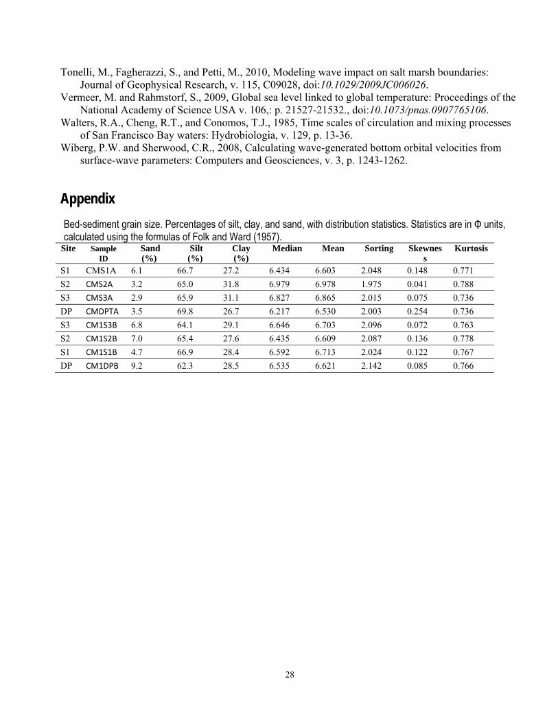
Bed-sediment grain size The ability of waves and currents to mobilize or erode bed sediment strongly depends on grain size and other bed properties (Stevens and others, 2006). On January 28 and March 18, 2010 we collected bed-sediment samples to determine grain-size distribution adjacent to each of the four stations in Corte Madera Bay (Table 3) from a small boat using a petite Ponar grab sampler. The top 2 cm of each sample was retained for analysis. Grain size distribution (¼ phi (φ) size classes) was determined using standard techniques. Both the sand fraction (2 mm – 63 µm) and fine fraction (< 63 µm) were analyzed with a Beckman Coulter model LS230 laser-diffraction particle analyzer.

Time and direction conventions Unless otherwise noted, all times in this report are in Universal Time, Coordinated (UTC) and

altitudes are referenced to a vertical datum of MLLW. For wind and waves, compass directions follow the meteorologic convention; for example, easterly winds or waves are from the east and have an azimuth of 90º. For currents, however, compass directions indicate the direction of flow, and so an eastward flowing current has an azimuthof 90º.

Results

Conditions during deployment The data collection period spanned 61 days, encompassing more than two full spring-neap cycles (fig. 4A). Instruments were deployed immediately after the largest storm of the winter, which occurred January 19-20, 2010. As a result, freshwater inflow from the Sacramento-San Joaquin Delta into northern San Francisco Bay (referred to as Delta outflow) was rising sharply when the instruments were deployed on January 22, and peaked during the first week of data collection (fig. 4B). Winds during the study period were typical, with wind speeds mostly less than 5 m/s and direction generally from the north-northwest or south-southeast. Several periods of stronger (5-8 m/s) winds occurred, with south-southeasterly direction. During the large storm immediately before instrument deployment, there were sustained southerly winds of about 8 m/s, which had largely abated by January 22 (fig. 5).

8

Bed-sediment grain size Disaggregated bed sediment from all four stations was predominantly (>92 percent) silt, with a

small fraction of very fine sand. All samples had a bimodal distribution, with the largest peak at 40 µm and a smaller peak at 4-6 µm (fig. 6). The grain size distribution was quite consistent between stations and across the two sampling dates, except for the January 28 sample from DP, in which the 40-µm peak is greater than in the March 18 sample. Because DP is the closest station to the channel and January 28 immediately followed the peak in Delta outflow, the greater fraction of 40-µm particles may represent the contribution of fresh sediment supplied by rivers; however, additional sampling would be required to verify this hypothesis. Percentages sand, silt, and clay, as well as statistics for the grain size distributions, are presented in the appendix.

Tidal elevations Tidal elevations were determined at all stations from pressure measurements. For each station,

pressure data were corrected for atmospheric pressure, as measured at the Richmond Bridge meteorologic station (http://www.ndbc.noaa.gov/, station rcmc1) and the height of the pressure sensor above the bed. At the shallow stations (S1-S3), the height of the instrument above the bed was determined from the mean (during the deployment) distance to bed, as measured by the ADV, and the vertical distance between the ADV transducer and the pressure sensor, which was measured before deployment of the platforms. For the marsh stations, where we made no measurement of distance to bed, we used the height of the pressure sensor above the weight (6 cm), assuming that the weight sank

Figure 4. Tides and Delta outflow for January-March 2010. A, Water surface elevation (WSE) relative to MLLW at Richmond tide station 9414683 (http://tidesandcurrents.noaa.gov). B, Net Delta outflow index (NDOI) in cubic meters per second (http://www.water.ca.gov/dayflow/). Red boxes delineate study period.

9

Figure 5. Meteorologic conditions at Richmond meteorological station RCMC1 (http://www.ndbc.noaa.gov/) January-March 2010. A, Wind speed. B, Wind direction. C, Atmospheric pressure. and D, Air temperature. Red dots in figure 6B, direction for wind speeds greater than 7 m/s. Red box delineates study period.

in to the top of its 5-cm thickness. Although measured depths were not corrected for settling of platforms during the deployment, we consider this a minor source of error because the variation during the deployment in distance to bed (measured by the ADVs), which reflects the combination of settling, erosion, and deposition beneath the tripod, was less than 6 cm at all shallow stations.

Tidal elevations at the shallow and marsh stations over 15 days are plotted in figure 7A. The tidal signal is truncated at the marsh stations, which were dry at low tide. Water depths below the sensor are plotted as 6 cm (the height of the pressure sensor above the bed). In general, the tidal elevations measured at all stations correspond well. Because the sensor at M1 was stationary, we relied on the difference in water depth between stations M2 and M1 (fig. 7B) to determine when the pressure sensor at M2 was moved and (or) tipped over. During each tidal cycle the difference ranges from close to zero,

10

when both sensors are exposed to air at low tide, to a relatively constant value corresponding to the difference in elevation between the two stations. The data indicate that the M2 sensor elevation was constant until February 6, when it decreased by approximately 5 cm, and that a second decrease occurred on February 10. The total change in elevation was approximately 7 cm, which can be accounted for by the tipping over of the pressure-sensor mount. The bathymetry is nearly flat between the deployed and retrieved locations. The largest differences in depth between M1 and M2 were caused by the tsunami originating in Chile at 0630 UTC February 27, 2010, which reached the northern California coast approximately 15 hours later. The tsunami waves were not fully resolved, owing to the 15-minute sampling interval, but elevated water-surface elevations as well as anomalous fluctuations as great as 20 cm, were measured for about 48 hours after the arrival of the tsunami (fig. 8A).

Figure 6. Grain-size distribution in top 2 cm of grab samples collected at S1-S3 and DP on January 28 and March 18, 2010. A, Station S1. B, Station S2. C, Station S3. D, Station DP.

11

Figure 7. A, Tidal elevations measured at the three ADV stations, M1, and M2, from January 25 to February 8, 2010. B, Difference in water depth between stations M2 and M1; difference is near zero when tidal elevation is below both sensors. Depths are calculated from pressure data and have been corrected for atmospheric pressure measured at station RCMC1 (fig. 1).

Temperature and salinity Water temperatures increased over the deployment period as spring progressed (fig.8B). Diurnal

variation in water temperature was greater within Corte Madera Bay (station S2) than in the channel (station DP), because the shallow waters of the Bay are more strongly influenced by air temperatures. Early in the deployment at station DP, water temperatures were higher near the bed, which is more influenced by ocean water, than at the surface, which is more influenced by Delta outflows. Subsequently surface and deep temperatures tracked one another closely until the last week of the study, when surface temperatures exceeded near-bed temperatures.

Both the tidal cycle variation and the vertical stratification in salinity at DP were greater early in the study period, when Delta outflow was high, than later (fig. 8C). In addition, vertical stratification was less during spring tides than during neap tides, attributable to greater tidally driven vertical mixing during spring tides. In general, salinities within Corte Madera Bay (fig. 8, station S2) were more similar to the near-surface than to the near-bed salinities at DP. Early in the deployment, the salinity at S2

12

varied by as much as 10 psu over the course of spring diurnal tidal cycles (Jan. 29-Feb. 4), despite the weak tidal currents within Corte Madera Bay. This indicates that horizontal gradients in salinity were strong and likely influenced circulation. The occasional dips in salinity at S2 (for example, on February 24) are likely due to local input of fresh water from Corte Madera creek.

Figure 8. Time series from January 22 to March 24, 2010 of A, depth at S2 showing tidal fluctuations, and B, temperature and C, salinity, 1 m below the water surface and 0.5 m above the bed (mab) at DP, and 0.5 mab at S2.

13

Currents Tidal currents at DP were aligned with the main channel (fig. 9D). Variation along the principal

axis (azimuth 19˚-199˚) accounted for more than 85 percent of the total variation in tidal currents. The amplitude of spring-tide depth-averaged currents was approximately 80 cm/s. Current speeds were greater during ebb than flood tides. During strong ebb tides, along-channel currents were significantly greater at the surface than near the bed, whereas during flood tides there was less variation with depth (fig. 10A).

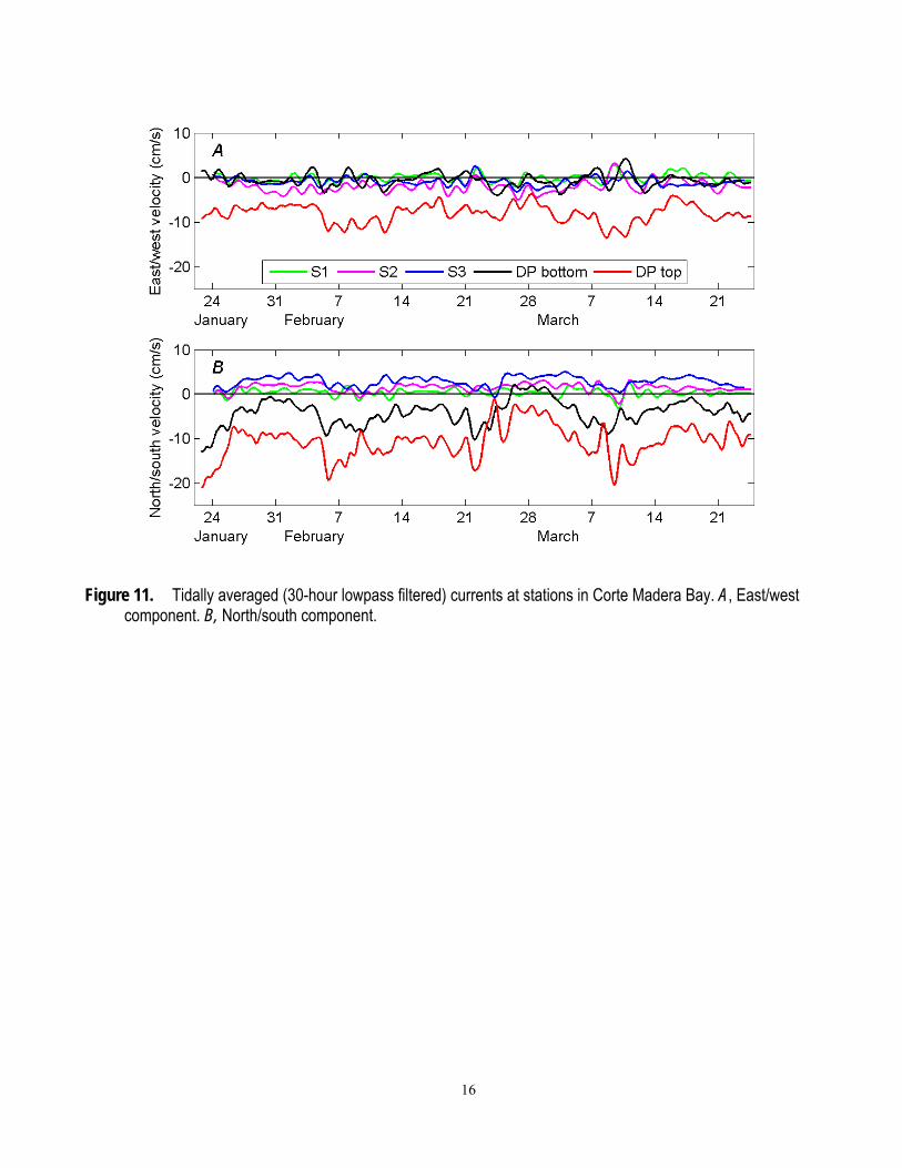
Tidally averaged currents were determined for all stations by filtering the velocity data with a low-pass (30-h stopband, 40-h passband) Butterworth filter. At DP, tidally averaged currents were southwestward near the surface, and southward near the bed (figs 11, 12B). They were stronger near the surface than near the bed, and stronger during spring than neap tides. We attribute the down-estuary (southerly) component of the tidally averaged flow to the elevated Delta outflows during the study period. The westerly component near the surface results from density-driven pulses of cross-channel flow into Corte Madera Bay in the upper water column during the transition from ebb to flood tides (fig. 10B), caused by the lower salinities at DP than in Corte Madera Bay (fig. 8C).

At the stations within Corte Madera Bay (S1-S3), flood-tide currents were northwestward and ebb tide currents were southeastward (figs. 9, 12). The westerly component was greatest at station S2. The amplitude of spring-tide currents decreased with distance into the bay, from 30 cm/s at station S3 to 10 cm/s at S1. Tidally averaged currents were also northwestward (into Corte Madera Bay) and were strongest during spring tides (fig. 11). During weak neap tides the currents briefly reversed to southeastward (for example, on Feb. 22 and Mar. 9). Tidally-averaged currents in Corte Madera Bay were 2 to 4 times weaker than at DP, and were weakest at the shallowest station (fig. 12B). Commonly, flow into an embayment like Corte Madera Bay is more focused into a jet than are ebb flows, which are more dispersed along the cross-section (Fisher and others., 1979). The net inward flow at stations S1 – S3, which were located along the axis of the embayment, is consistent with this pattern.

Waves Wave conditions during the study are summarized in time series of wave statistics from station

DP (fig. 13). During the largest wave events, significant wave height (Hs ) at station DP exceeded 0.5 m, wave period was approximately 3 s, and wave azimuth was approximately 150˚. During these events, energy at low frequencies (periods > 5 s) was negligible, indicating that waves were locally generated by wind, rather than ocean swell (fig. 13E). During wave events with Hs > 0.3 m (red dots in fig. 13), wave period and azimuth were quite consistent (2-4 s and 120º-150º, respectively), although these parameters vary widely over the full time series. To examine wave attenuation within Corte Madera Bay and Marsh, we focus on the three largest wave events during the study, which occurred on February 5, 24, and 26-27, 2010.

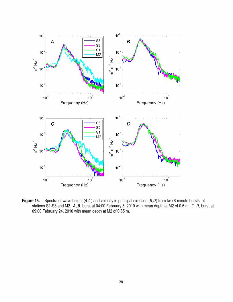
Water depths at stations S1-S3 and M2 from the burst at 0400 UTC during the February 5 wave event (fig. 14) illustrate the short-term temporal variability in wave heights, which is not captured in the burst statistics. We note that the range of wave heights is reduced at M2, presumably due to breaking of the largest waves. Spectra of velocity and pressure from this burst (figs. 15A, 15B) show that energy is transferred from lower to higher frequencies, indicative of wave breaking, as the waves travel into shallower water at station M2. The peak frequency decreases slightly as water depth decreases, but the spread of frequencies increases considerably. In a burst collected at a higher tidal stage this effect is less pronounced (figs. 15C, 15D)

14

Figure 9. Tidal currents at 30-minute intervals from February 1 to February 6, 2010, showing variation from spring to neap tides. A, Station S1, 0.2 mab. B, Station S2, 0.3 mab. C, Station S3, 0.3 mab. D, Station DP, depth averaged.

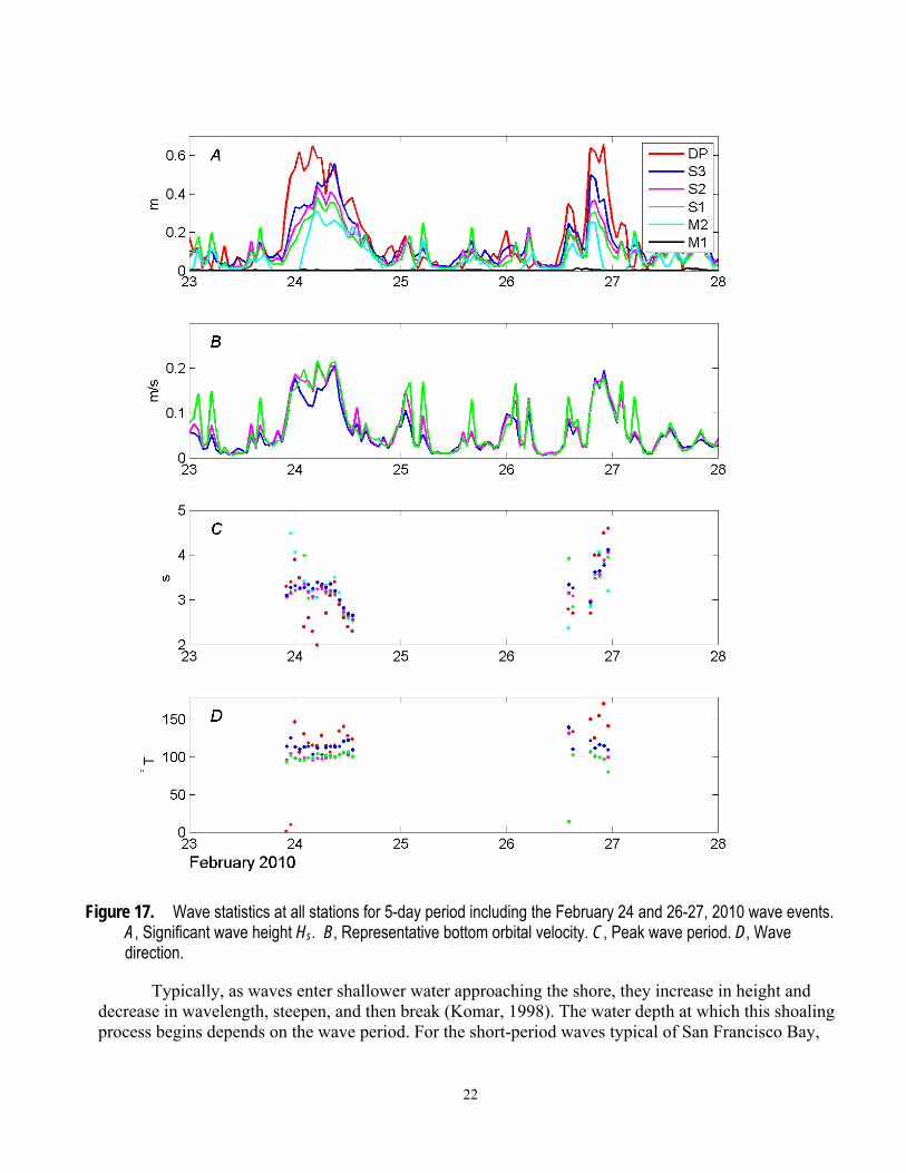
As waves penetrated into Corte Madera Bay (stations S1-S3), wave direction veered eastward owing to refraction, and wave height decreased, but wave period did not change significantly (figs. 16, 17). Wave heights at M2, the station immediately bayward of the marsh, followed this pattern, except that Hs dropped to zero when tidal elevations were below the sensor (for example, on Feb. 4 at 20:00, Feb. 24 at 00:00, and Feb. 27 at 00:00). At station M1, 150 m inshore of the marsh edge, wave heights

15

were negligible. The greatest Hs measured at M1 was 2.3 cm on February 28 at 20:00 , when Hs at M2 was 22.3 cm, and the tidal elevation was 2.1 m MLLW. At this time, water levels in the bay were influenced by the Chile tsunami, which may have contributed indirectly to the fluctuations in water surface elevation at M1 (although the calculation of Hs was based on frequencies between 0.125 and 0.5 Hz, much higher than the tsunami frequency). The maximum Hs measured at M1 outside of the period influenced by the tsunami was 1.5 cm.

Although wave height decreased substantially toward shore, bottom orbital velocity at stations S1-S3 was remarkably constant (for example, figs. 16A, 16B, Feb. 5, and figs. 17A, 17B, Feb. 26), except for brief peaks at the shallowest station at low tide. The near-constant bottom orbital velocities result from two opposing tendencies: a decrease in orbital velocity associated with lower wave height, and an increase in bottom orbital velocity due to the decrease in depth, because the orbital velocities of these short period waves decay with distance below the surface. Bed shear stress varies with the square of bottom orbital velocity, so our results indicate that the potential for wave-driven sediment resuspension is similar at the three stations, which represent much of Corte Madera Bay.

Figure 10. Current profiles from ADCP at station DP for March 1-7, 2010. A, Along-channel component. B, Cross-channel component. Azimuths are 19˚(upstream) for positive along-channel velocities and 289˚ (toward Corte Madera) for positive cross-channel velocities.

16

Figure 11. Tidally averaged (30-hour lowpass filtered) currents at stations in Corte Madera Bay. A, East/west component. B, North/south component.

17

Figure 12. A, Speed and direction of spring-tide tidal currents at stations DP-T (depth averaged), S1, S2, and S3 (compare to fig. 9). B, Speed and direction of mean tidally averaged currents at DP-T near surface (dashed) and near bottom (solid), and at S1, S2, and S3 (compare to fig. 11).

.

18

Figure 13. Time series of wave statistics and tidal elevations from ADCP at station DP-T. A, Significant wave height. B, Peak wave period. C, Wave direction. D, Water depth, and E, Nondirectional spectra of wave energy. Red dots indicate Hs> 0.3 m.

19

Figure 14. High-frequency water depths from a burst at 0400 February 5, 2010 UTC at stations S3 (A), S2 (B), S1 (C), and M2 (D).

20

Figure 15. Spectra of wave height (A,C) and velocity in principal direction (B,D) from two 8-minute bursts, at stations S1-S3 and M2. A, B, burst at 04:00 February 5, 2010 with mean depth at M2 of 0.6 m. C, D, burst at 09:00 February 24, 2010 with mean depth at M2 of 0.85 m.

21

Figure 16. Wave statistics at all stations for 5-day period including the February 5, 2010 wave event. A, Significant wave height Hs. B, Representative bottom orbital velocity. C, Peak wave period. D, Wave direction.

22

Figure 17. Wave statistics at all stations for 5-day period including the February 24 and 26-27, 2010 wave events. A, Significant wave height Hs. B, Representative bottom orbital velocity. C, Peak wave period. D, Wave direction.

Typically, as waves enter shallower water approaching the shore, they increase in height and decrease in wavelength, steepen, and then break (Komar, 1998). The water depth at which this shoaling process begins depends on the wave period. For the short-period waves typical of San Francisco Bay,

23

shoaling is restricted to very shallow water: for example, less than 0.7 m for 3-s wave periods (based on the definition of shallow-water waves, ∞ 20⁄ , where L∞ is the deep-water wavelength from linear wave theory, calculated as ∞ 2 ⁄ , T is the wave period, and g is gravitational acceleration). In the study area (fig. 1) the shoaling depth was always inshore of stations S3 and S2, and inshore of S1 for tidal elevations greater than 0.2 m MLLW.

Waves only reach station M1 when the marsh plain bayward of the station is inundated, which occurs at tidal elevations greater than about 1.6 m MLLW (15 percent of the time during the study period). Waves break when their height H exceeds approximately 0.78 h, where h is the water depth (Komar, 1998). Thus, at a tidal elevation of 2 m MLLW (close to the maximum; see fig. 4A), incident waves with H>0.3 m would break simply owing to the shallow water depth over the marsh, and the maximum possible wave height decreases to zero for a tidal elevation of 1.6 m. Pickleweed and other vegetation extend at least 20 cm above the marsh plain, further impeding wave propagation and potentially causing waves to break. Note that in this study, fewer than 10 of 1456 bursts (0.7 percent) had Hs > 0.3 m at DP and a tidal elevation greater than 1.6 m MLLW. This low rate of incidence limits our ability to assess wave attenuation over the marsh but also provides an indication of the frequency of such conditions in a typical winter.

To characterize the attenuation or damping of waves within the study area we use a normalized wave height, calculated as the ratio of Hs at each station to Hs at station DP:

1 /

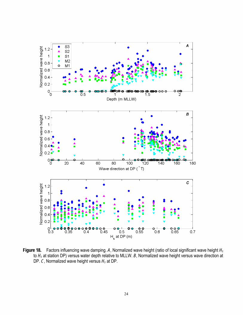
where A is the fractional attenuation at each station. As illustrated in figures 16A and 17A, attenuation increased with distance from DP. Attenuation was also influenced by tidal elevation and wave direction but does not appear to depend on wave height (fig. 18). Wave period did not affect attenuation (not shown). The low normalized wave heights at M2 between tidal elevations of 0.67 m (inundation level) and approximately 1 m MLLW are influenced by wave breaking due to shallow water depths, which is not typically considered attenuation (fig. 18A). Depth limitation was insignificant at the other stations (H/h was always substantially less than 0.7). Normalized wave height approaches 1 between tidal elevations of 1.1 and 1.6 m MLLW (fig. 18A). At these depths, the mudflats are inundated but the marsh plain is not, so the decrease in attenuation may result from wave reflection off the marsh scarp, as numerical models predict for marshes with steep banks (Tonelli and others, 2010).

Normalized wave height was maximum, and attenuation minimum, when the direction of waves at DP was most closely aligned with the axis of Corte Madera Bay, azimuth 110˚ - 140˚ (fig. 18B). Within this range, wave height at S3 is close to, and sometimes exceeds, that at DP, but wave height at the shallowest stations (S1 and M2) is typically reduced by about 40 percent. Outside of this range of wave directions, waves within Corte Madera Bay are more strongly damped because some of the wave energy reaching station DP is not refracted into the bay.

Ferry wakes Although our data collection was designed to characterize wind waves, the data include many examples of ferry wakes. Figure 19 shows several examples of wakes and their propagation across the study area. The characteristics of the wakes were influenced by tidal stage. At low tide (figs. 19A, 19B), wave steepening occurred as the wakes reach shallower stations, and the wakes do not reach the marsh edge. At high tides, when the marsh plain is inundated (figs. 19E, 19F), wakes propagate to the marsh edge (station M2), and in some cases the wake is amplified as it reaches the shallower stations (fig. 19F). Only small-amplitude (< 5 cm), low-frequency oscillations were observed at M1. The largest and

24

Figure 18. Factors influencing wave damping. A, Normalized wave height (ratio of local significant wave height Hs to Hs at station DP) versus water depth relative to MLLW. B, Normalized wave height versus wave direction at DP. C, Normalized wave height versus Hs at DP.

25

Figure 19. Examples of ferry wakes at low tide (A, B), mid tide (C, D) and high tide (E, F). Water depths at S3 have been offset by -0.5 m to facilitate comparison between stations.

26

steepest wakes reaching the marsh edge occurred at intermediate tidal elevations (figs. 19C, 19D). Some of these complex waveforms may result from the interaction of two wakes approaching from different angles. For example, the short travel times between stations for the second wake in figure 19C indicates that the propagation direction is closer to shore-parallel than shore-perpendicular, and the wave at M2 may represent the interaction of the two wakes. At the intermediate tidal elevations of figures 19C and 19D, the marsh plain is not inundated but the sensor at M1 is submerged by the tidal creek, in which low-frequency water-surface oscillations occurred.

Summary and Conclusions Currents and wave properties were measured in a cross-shore transect from outside Corte

Madera Bay to 150 m landward of the marsh edge from January 23 to March 22, 2010 to characterize currents, waves, and wave attenuation. The deployment captured three storm events with significant wave heights greater than 0.4 m at the deepest station (-7 m MLLW). At the station 150 m landward of the marsh edge, the maximum significant wave height was 2.3 cm, indicating that damping of the waves was essentially complete. In addition, wave height decreased by as much as 80 percent as waves propagated across the shallows of Corte Madera Bay. Mean attenuation for waves with Hs>0.3 m at station DP was 30 percent at station S3, 47 percent at S2, 55 percent at S1, 66 percent at M2, and 99.3 percent at M1 (where percentage of attenuation is calculated as % 100 1 ). In calculating

mean attenuation for the marsh stations, bursts with water level below the sensor (at M2) or below the marsh plain elevation (at M1) were excluded. Wave attenuation was lowest when the wave direction (at station DP) was aligned with the axis of Corte Madera Bay, and at intermediate tidal elevations. The dependence on direction indicates that some of the reduction in wave height reflected in the mean attenuation values is caused by sheltering. For waves directed along the bay’s axis, attenuation over the mudflats was nonetheless substantial, ranging from 20 to 60 percent at M2.

The lower part of the marsh is inundated when tidal elevations exceed approximately 1.6 m MLLW, which occurred 15 percent of the time during the study. Similarly, the marsh was inundated for 15 percent of the time that offshore wave heights exceeded 0.3 m. At lower tidal elevations, waves break against the edge of the marsh before reaching the marsh. Thus marsh vegetation plays a role in attenuating waves only during storms that occur at high tide. In addition, the low water depths over the marsh at high tide cause all but the smallest waves to break. Thus the wave damping that occurred over the marsh was a combination of bathymetric effects that are independent of vegetation, and the vegetative drag effect typically considered marsh attenuation.

Ferry wakes arrive at the marsh edge regularly and appear to present the maximum potential for erosion at intermediate tidal elevations, when wakes break against the marsh scarp, and shallow water at the marsh edge causes the leading edges of wakes to steepen. Some wakes were amplified as they approached shore. However, the largest observed wakes were no larger than significant wave heights that persisted at the marsh edge for several hours during the February 2010 storm events.

Although the damping of waves within Corte Madera Marsh during winter 2010 can be attributed largely to bathymetry, the marsh nonetheless serves as a barrier protecting the shoreline from waves. In the absence of the marsh, the wave forces currently eroding the marsh edge would be impacting a developed shoreline. The wave events from January 22 to March 23, 2010 were moderate, likely to occur each winter. The essentially complete damping within 150 m of the marsh edge observed during these events is not necessarily a good predictor for extreme events. During extreme events with greater wave heights and higher water surface elevations due to storm surge, attenuation by marsh vegetation is likely to be a more important component of total wave damping.

27

Acknowledgments Thanks to Joanne Ferreira, Pete DalFerro, Tim Elfers, Jamie Grover, Rob Wyland, Peter

Harkins, and Shandy Buckley of the US Geological Survey (USGS) for excellent field support. Adam Parris (PWA) and Wendy Goodfriend of BCDC coordinated with the Environmental Protection Agency (EPA), the Corte Madera Ecological Reserve, and other scientists working in Corte Madera Marsh. The concept for this study was initiated by Dave Cacchione (CME), Bruce Jaffe (USGS), and Adam Parris. This report benefited from thoughtful reviews by Andrew Stevens and Renee Takesue of the USGS. Theresa Fregosa (USGS) prepared figures 1 and 13. This study is part of the Innovative Wetland Adaptation in the Lower Corte Madera Creek Watershed Project initiated by BCDC and funded by EPA; additional support was provided by the USGS Coastal and Marine Geology Program.

References Cited Atwater, B.F., 1979, History, landforms, and vegetation of the estuary’s tidal marshes, in Conomos,

T.J., ed., San Francisco Bay: The urbanized estuary: 58th Annual Meeting, Pacific Division, American Association of the Advancement of Science, June 1977, San Francisco.

Conomos, T.J., Smith, R.E., and Gartner, J.W., 1985, Environmental setting of San Francisco Bay: Hydrobiologia, v. 129, p. 1-12.

Feagin, R.A., Lozada-Bernard, S.M., Ravens, T.M., Moller, I., Yaeger, K.M., and Baird, A.H., 2009, Does vegetation prevent wave erosion of salt marsh edges?: Proceedings of the National Academy of Sciences USA, v. 106, no. 25, p. 10109-10113, doi:10.1073/pnas.0901297106.

Fischer, H.B., List, J.E., Koh, R.C.Y., Imberger, J., and Brooks, N.H., 1979. Mixing in inland and coastal waters: Academic Press, Inc., San Diego CA, 483 p.

Folk, R.L. and Ward, W.C., 1957, Brazos River bar, a study in the significance of grain-size parameters: Journal of Sedimentary Petrology, v. 27, p. 3-27.

Komar, P. D., 1998, Beach processes and sedimentation. 2nd edition. Prentice-Hall Inc., Upper Saddle River, N.J., 544 p.

Le Hir, P., Roberts, W., Cazaillet, O., Christie, M., Bassoullet, P., and Bacher, C., 2000, Characterization of intertidal flat hydrodynamics: Continental Shelf Research, v. 20, p. 1433-1459.

Madsen, O.S., 1994, Spectral wave-current bottom boundary layer flows, in Coastal Engineering 1994: Proceedings, 24th International Conference, Coastal Engineering Research Council: American Society of Civil Engineers, Kobe, Japan. p. 384-398.

Moller, I., Spencer, T., French, J.R., Leggett, D.J., and Dixon, M.,1999, Wave transformation over salt marshes: A field and numerical modeling study from north Norfolk, England: Estuarine, Coastal and Shelf Science, v. 49, p. 411-426.

Moller, I., 2006, Quantifying saltmarsh vegetation and its effect on wave height dissipation: Results from a UK East coast saltmarsh: Estuarine, Coastal and Shelf Science, v. 60, p. 337-351.

Monroe, M, Olofson PR, Collins JN, Grossinger RM, Haltiner J, Wilcox C., 1999, Baylands Ecosystem Habitat Goals: U.S. Environmental Protection Agency, San Francisco CA/San Francisco Bay Regional Water Quality Control Board, Oakland CA, USA.

Philip Williams & Associates, Ltd. and Faber, P.M., 2004,. Design guidelines for tidal wetland restoration in San Francisco Bay:the Bay Institute and California State Coastal Conservancy, Oakland, CA. 83 p.

Stevens, A.W., Wheatcroft, R.A., and Wiberg, P.L., 2006, Seabed properties and sediment erodibility along the western Adriatic margin, Italy: Continental Shelf Research, v. 27, p. 400-416, doi:10.1016/j.csr.2005.09.009.

28

Tonelli, M., Fagherazzi, S., and Petti, M., 2010, Modeling wave impact on salt marsh boundaries: Journal of Geophysical Research, v. 115, C09028, doi:10.1029/2009JC006026.

Vermeer, M. and Rahmstorf, S., 2009, Global sea level linked to global temperature: Proceedings of the National Academy of Science USA v. 106,: p. 21527-21532., doi:10.1073/pnas.0907765106.

Walters, R.A., Cheng, R.T., and Conomos, T.J., 1985, Time scales of circulation and mixing processes of San Francisco Bay waters: Hydrobiologia, v. 129, p. 13-36.

Wiberg, P.W. and Sherwood, C.R., 2008, Calculating wave-generated bottom orbital velocities from surface-wave parameters: Computers and Geosciences, v. 3, p. 1243-1262.

Appendix

Bed-sediment grain size. Percentages of silt, clay, and sand, with distribution statistics. Statistics are in Φ units, calculated using the formulas of Folk and Ward (1957).

Site Sample ID

Sand (%)

Silt (%)

Clay(%)

Median Mean Sorting Skewness

Kurtosis

S1 CMS1A 6.1 66.7 27.2 6.434 6.603 2.048 0.148 0.771

S2 CMS2A  3.2 65.0 31.8 6.979 6.978 1.975 0.041 0.788

S3 CMS3A  2.9 65.9 31.1 6.827 6.865 2.015 0.075 0.736

DP CMDPTA  3.5 69.8 26.7 6.217 6.530 2.003 0.254 0.736

S3 CM1S3B  6.8 64.1 29.1 6.646 6.703 2.096 0.072 0.763

S2 CM1S2B  7.0 65.4 27.6 6.435 6.609 2.087 0.136 0.778

S1 CM1S1B  4.7 66.9 28.4 6.592 6.713 2.024 0.122 0.767

DP CM1DPB  9.2 62.3 28.5 6.535 6.621 2.142 0.085 0.766