wave breaking onset and strength for two …ltalley/sio219/banner_peirson_jfm2007.pdf · wave...

J. Fluid Mech. (2007), vol. 585, pp. 93–115. c© 2007 Cambridge University Press

doi:10.1017/S0022112007006568 Printed in the United Kingdom

93

Wave breaking onset and strength fortwo-dimensional deep-water wave groups

MICHAEL L. BANNER1 AND WILLIAM L. PEIRSON2

1School of Mathematics and Statistics, The University of New South Wales, Sydney 2052, Australia2Water Research Laboratory, School of Civil and Environmental Engineering,

The University of New South Wales, Sydney 2052, Australia

(Received 1 June 2006 and in revised form 8 March 2007)

The numerical study of J. Song & M. L. Banner (J. Phys. Oceanogr. vol. 32, 2002,p. 254) proposed a generic threshold parameter for predicting the onset of breakingwithin two-dimensional groups of deep-water gravity waves. Their parameter providesa non-dimensional measure of the wave energy convergence rate and geometricalsteepening at the maximum of an evolving nonlinear wave group. They also suggestedthat this parameter might control the strength of breaking events. The present paperpresents the results of a detailed laboratory observational study aimed at validatingtheir proposals.

For the breaking onset phase of this study, wave potential energy was measured atsuccessive local envelope maxima of nonlinear deep-water wave groups propagatingalong a laboratory wave tank. These local maxima correspond alternately to wavegroup geometries with the group maximum occurring at an extreme carrier wavecrest elevation, followed by an extreme carrier wave trough depression. As thenonlinearity increases, these crest and trough maxima can have markedly differentlocal energy densities owing to the strong crest–trough asymmetry. The local totalenergy density was reconstituted from the potential energy measurements, and madedimensionless using the square of the local (carrier wave) wavenumber. A meannon-dimensional growth rate reflecting the rate of focusing of wave energy at theenvelope maximum was obtained by smoothing the local fluctuations.

For the cases of idealized nonlinear wave groups investigated, the observationsconfirmed the evolutionary trends of the modelling results of Song & Banner (2002)with regard to predicting breaking onset. The measurements confirmed the proposedcommon breaking threshold growth rate of 0.0014 ± 0.0001, as well as the predictedkey evolution times: the time taken to reach the energy maximum for recurrencecases; and the time to reach the breaking threshold and then breaking onset, forbreaking cases.

After the initiation and subsequent cessation of breaking, the measured wave packetmean energy losses and loss rates associated with breaking produced an unexpectedfinding: the post-breaking mean wave energy did not decrease to the mean energy levelcorresponding to maximum recurrence, but remained significantly higher. Therefore,pre-breaking absolute wave energy or mean steepness do not appear to be the mostfundamental determinants of post-breaking wave packet energy density.

However, the dependence of the fractional breaking energy loss of wave packets onthe parametric growth rate just before breaking onset proposed by Song & Banner(2002) was found to provide a plausible collapse to our laboratory data sets, withinthe experimental uncertainties. Further, when the results for the energy loss rate perunit width of breaking front were expressed in terms of a breaker strength parameterb multiplying the fifth power of the wave speed, it is found that b was also strongly

94 M. L. Banner and W. L. Peirson

correlated with the parametric growth rate just before breaking. Measured values ofb obtained in this investigation ranged systematically from 8 × 10−5 to 1.2 × 10−3.These are comparable with open ocean estimates reported in recent field studies.

1. IntroductionBreaking of dominant ocean wind waves in the form of large whitecaps is a familiar

occurrence associated with strong wind forcing conditions at sea. Through theiroverturning of the air–sea interface, such breaking events (as well as those of shorterbreaking waves) profoundly influence the dynamics and thermodynamics of the upperocean and marine atmospheric boundary layer, while their impact forcing provides thegreatest safety challenge to offshore shipping and coastal structures. Consequencesof breaking in the upper ocean surface layer include greatly enhanced turbulencedissipation rates in the near-surface region (e.g. Terray et al. 1996; Gemmrich &Farmer 2004). In the atmospheric marine boundary layer, increased waveform dragcan result from the separated air flow over breaking waves, together with augmentedsea spray, bubbles and acoustic underwater noise, as well as enhanced microwavebackscatter and emissivity. These numerous and diverse aspects of wave breaking aredescribed in greater detail in, for example, Banner & Peregrine (1993); Thorpe (1993)and Melville (1996).

Despite the widespread occurrence of breaking waves at sea, an understanding ofthe mechanisms that determine the onset and strength of breaking events has beenelusive ever since water waves have been studied scientifically. Identifying a robustthreshold variable that determines the onset of breaking for deep-water waves hasremained a problem for many decades. Various breaking threshold criteria have beenproposed based on local wave geometrical or kinematical properties such as wavesteepness, crest fluid velocities and acceleration, and Stansell & MacFarlane (2002)provides a critical appraisal of this kinematic approach. However, breaking criteriabased on such local properties do not appear to be universally applicable, as evidencedin a number of laboratory and field observations. For example, the comprehensivefield study of Holthuijsen & Herbers (1986) highlights the inability to distinguishbreaking events on the basis of local wave steepness. In any event, it may be arguedthat such breaking criteria do not provide much insight into the underlying dynamicsthat determines the onset and strength of wave breaking, a shortcoming shared bystatistically based, broader spectral variants of these criteria (e.g. Papadimitrakis et al.1988).

Of potential significance to the dynamics underlying wave breaking have beenfield observations associating wave breaking with wave group structure, particularlythose of Donelan, Longuet-Higgins & Turner (1972) and subsequently Holthuijsen &Herbers (1986). Furthermore, wave group structure is a conspicuous feature of oceanwave height records and a significant amount of literature exists on this topic.In the present context, the statistics of wave groups (e.g. Longuet-Higgins 1984)and the occurrence of extreme waves in wave groups (e.g. Phillips, Gu & Donelan1993; Osborne, Onorato & Serio 2000) are of particular relevance. Complementarylaboratory observational studies have investigated the unforced (zero wind) evolutionof two-dimensional nonlinear wave groups (e.g. Melville 1982, 1983; Rapp & Melville1990; Kway, Loh & Chan 1998; Tulin & Waseda 1999). These papers, however, donot address the underlying dynamical underpinnings of wave breaking onset. There

Wave breaking onset and strength 95

has also been strong interest in studying nonlinear modulational processes throughmodel equations, such as the nonlinear Schrodinger equation and its higher-ordervariants (e.g. Dysthe 1979; Dias & Kharif 1999). While well-suited to examiningmany aspects of wave group behaviour, such model equations cannot describe theonset of wave breaking, which requires the exact (Euler) equation formulation withfully nonlinear free-surface boundary conditions.

Complementary to these theoretical developments, recent numerical studies havebeen made of the evolution of unforced two-dimensional nonlinear wavetrains beyondthe linear perturbation instability stage. These calculations reveal a complex evolutionto recurrence or breaking that highlights the fundamental role played by nonlinearintra-wave group dynamics (e.g. Dold & Peregrine 1986; Tulin & Li 1992; Banner &Tian 1998).

The present laboratory investigation seeks to advance present understanding of twofundamental aspects of group-related deep-water wave breaking behaviour: breakinginitiation, and subsequent loss of energy from the wave field.

1.1. Onset of wave breaking

Song & Banner (2002 hereinafter referred to as SB) used a wave-group-following(WGF) approach to investigate numerically the evolution of unforced two-dimen-sional nonlinear wave groups with different initial wave group structure. SB soughtto identify the difference between evolution to recurrence and to breaking onset, interms of the rate of mean wave energy convergence and geometrical steepening atthe maximum of wave groups, when travelling with these wave group maxima. Aftercalculating the long-term evolution of the maximum of the local energy density ofwave groups, with suitable post-processing they tracked the envelope maximum of thewave group energy and calculated an associated non-dimensional parametric meangrowth rate δ, defined by

δ(t) =1

ωc

D〈µ〉Dt

, (1)

where D/Dt is the rate of change following the wave group whose initial mean carrierwave frequency is ωc, µ =Ek2 is a non-dimensional variable reflecting the local waveenergy and wavenumber behaviour. Here, E is the depth-integrated local total energydensity (after division by ρwg) and k is the local wavenumber. The local mean valueof µ averaged over several carrier wave periods is denoted by 〈µ(t)〉. Following SB,ωc was taken as the mean frequency of the two spectral modes in case II wave groupsand as the mean paddle frequency (ωp) for the case III wave groups. Definitionsof these wave group geometries are given in § 2.2. The mean carrier wave periodT =2π/ωc.

The growth rate δ reflects a mean energy convergence rate towards, or away from,the wave group energy maximum, associated with nonlinear interactions of waveenergy from other parts of the wave group, as measured by an observer travellingwith the wave group. It also reflects the steepening of the maximal carrier waveformassociated with the increased local carrier wavenumber. However, as discussed indetail in § 4b of SB, the energy maximum of a wave group oscillates as it growsduring the evolution, owing to the crest–trough asymmetry associated with Stokeswaves, and these fast oscillations must be filtered out to obtain the associated meanparametric growth rate δ. For the ensemble of different structures and sizes of wavegroups they investigated, SB found that this dynamically based mean growth ratehad a common threshold of [1.4 ± 0.1] × 10−3 that distinguished evolution of thegroup to recurrence without breaking, from evolution in which initiation of breaking


occurs. In a companion paper, Banner & Song (2002) extended that unforced studyto strongly wind-driven cases, reporting that the hydrodynamics of nonlinear wavegroups continued to dominate the breaking onset process even for relatively strongwind forcing. Compared to previously proposed breaking thresholds, this dynamicallybased approach contributes a more complete physical perspective, both long-term andshort-term, of the evolution to breaking and provides an earlier and more decisiveindicator for the onset of breaking.

The present paper describes the results of our detailed laboratory study to validatethe proposed SB breaking threshold growth rate and their suggested dependence ofbreaking energy loss on this growth rate just before breaking onset. To this end,detailed measurements were made of the evolution of the wave potential energydensity and relevant carrier wave properties in a laboratory wave flume for tworepresentative paddle-generated initial wave group geometries. The experiments weredesigned to reproduce conditions representing a subset of those in the calculations ofSB. From this data, the behaviour of the SB parametric growth rate parameter δ wascalculated using exactly the same methodology as in SB for direct comparison withtheir model results for breaking onset.

1.2. Strength of wave breaking

SB also proposed that the growth rate δbr just prior to breaking onset might providea dynamically based measure of the strength of breaking events, but the latter wasnot available from their computations, which terminated just after the actual onsetof breaking. The consequences of wave breaking remain major challenges in air–seainteraction modelling. We sought to extend present knowledge of breaking energylosses and loss rates beyond their dependence on the initial mean wave packetsteepness, as explored by, for example, Dold & Peregrine (1986), Thorpe (1993) andMelville (1994). To this end, we undertook a systematic study of how the post-breaking mean wave packet energy was correlated with the pre-breaking growth rateδbr explored by SB.

For the post-breaking phase, we also examined the breaking energy loss raterelationship proposed by Duncan (1981, 1983). Based on dimensional considerations,Duncan proposed that the energy loss rate per unit width of breaking front εL couldbe expressed in terms of a breaker strength coefficient b multiplying the fifth powerof the breaking wave speed cbr :

εL = bbrρwc5br

/g, (2)

where ρw is the water density. In (2), the unknown non-dimensional coefficient bbr

reflects the breaking ‘strength’ or ‘intensity’. Subsequent investigations have sought toquantify bbr and its parametric dependence (e.g. Phillips 1985; Melville 1994; Peirson &Banner 2000; Phillips, Pasner & Hansen 2001; Melville & Matusov 2002; Gemmrich2005). Present estimates for the breaking strength coefficient bbr from laboratoryand field measurements range over two orders of magnitude. From measurements ofenergy dissipated and breaker durations in the laboratory study of Loewen & Melville(1991), Melville (1994) reported a parametric dependence for bbr on the maximumpacket wave slope parameter S, where S =(Σan)kc is the maximal steepness of thediscrete Fourier wave amplitudes an in the wave packet, and kc is the mean packetwavenumber.

In the present study, we sought to refine the quantification of the breaking strengthcoefficient bbr , particularly its correlation with S and with the more intrinsic breakingparameter δbr . In the following sections, we describe the experimental facilities and


30 m0.

63m

Cantilevered flexibleplate wavemaker

Perforated plate/horsehair beach

Wave tank elevation(approx. scale 1:50)

Servo-controlledactuator

0.45

m

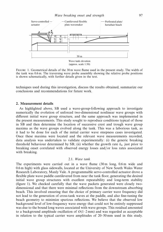
Figure 1. Geometrical details of the 30 m wave flume used in the present study. The width ofthe tank was 0.6m. The traversing wave probe assembly showing the relative probe positionsis shown schematically, with further details given in the text.

techniques used during this investigation, discuss the results obtained, summarize ourconclusions and recommendations for future work.

2. Measurement detailsAs highlighted above, SB used a wave-group-following approach to investigate

numerically the evolution of unforced two-dimensional nonlinear wave groups withdifferent initial wave group structure, and the same approach was implemented inthe present measurements. This study sought to reproduce conditions typical of thosein SB and then determine the location of successive crest and trough wave groupmaxima as the wave groups evolved along the tank. This was a laborious task, asit had to be done for each of the initial carrier wave steepness cases investigated.Once these maxima were located and the relevant wave measurements recorded,data analysis was undertaken to validate experimentally: (i) the generic breakingthreshold behaviour determined by SB; (ii) whether the growth rate δbr just prior tobreaking onset correlated with observed energy losses and/or loss rates associatedwith breaking.

2.1. Wave tank

The experiments were carried out in a wave flume (30 m long, 0.6 m wide and0.6 m high) with glass sidewalls, located at the University of New South Wales WaterResearch Laboratory, Manly Vale. A programmable servo-controlled actuator drove aflexible plate wave paddle cantilevered from near the tank floor, generating the desiredinitial wave group structures with excellent repeatability and long-term stability(figure 1). We checked carefully that the wave packets generated were closely two-dimensional and that there were minimal reflections from the downstream absorbingbeach. This involved ensuring that the choice of primary carrier wave frequency didnot lead to the generation of cross-tank waves at the paddle, and also fine-tuning thebeach geometry to minimize spurious reflections. We believe that the observed lowbackground level of low-frequency wave energy that could not be entirely suppressedwas due to the bound long waves associated with wave groups. This residual amountedto a background amplitude oscillation of O(1–2 mm) and was regarded as acceptablein relation to the typical carrier wave amplitudes of 20–50 mm used in this study.


There was an associated residual lateral sloshing inhomogeneity of the same order,with O(1–2 mm) amplitude.

2.2. Cases of initial wave groups investigated

We investigated cases based on two of the generic wave group structures reportedby SB. Because of finite tank length considerations, we chose the bimodal initialspectrum (case II) and the chirped wave packet (case III), and initially investigatedcases comprising five carrier waves in the initial spatial wave group. The case II wavegroups generated had an initial spectrum of the form

η = a0 cos(k0x) + εa0 cos

(N + 1

Nk0x − π

18

)with ε = 1, (3)

where a0 is the amplitude and N = 5 is the number of waves in the group. Thesmall phase shift, retained from Banner & Tian (1998), is inconsequential. Becauseof the well-known dispersive properties of deep-water gravity waves, the temporalsignal has 10 waves/group to generate this five-wave spatial group structure. Withan appropriate mean carrier wave frequency of 1.7 Hz, we were able to match closelythe computed wave group evolution within the constraints of our wave tank. Wesubsequently carried out measurements using a bimodal spectrum with N = 3 inorder to extend our measurement parameter space.

The case III wave groups had a more rapidly deforming geometry characteristic ofchirped wave packets where the carrier waves in the packet coalesce rapidly owing totheir different phase velocities. These wave packets were produced here, as with thechirped packets in SB, by driving the wavemaker with the motion

xp = −0.25Ap

(tanh

4ωpt

Nπ+ 1

)(1 − tanh

4(ωpt − 2Nπ)

Nπ

)sin[ωp(t − 0.018t2/2)], (4)

where t is time and N sets the number of carrier waves in the packet, Ap isproportional to the piston amplitude, ωp = (g/(2π/λ) tanh((2π/λ)h))1/2 is its angularfrequency, λ is the wavelength and h is the still-water depth. To simulate deep water,SB took the still-water depth near the wave paddle as h = 4 m, with λ= 2 m. For thecase III measurements, we chose a paddle frequency ωp comparable with the case IIwaves and used this in (3), as our tank was too short to accommodate the anticipatedevolution of a wavelength of λ= 2 m.

We note that the wave paddle mechanism installed in our facility was a bottom-cantilevered flexible plate with tapered stiffness, designed to be optimal for producingdeep-water waves with minimal settling distance. This was ideal for simulating theconditions of the case II (periodic domain) wave group evolution. However, it appearsto have created a mismatch for the case III wave groups, for which the SB model useda horizontal piston flat-plate paddle motion. We believe that this did not allow us toreproduce optimally the observational conditions for the case III wave groups with theinitial conditions of the SB model. The cantilevered flexible-plate generator provideswater particle orbital motions far closer to the exponentially decreasing with depthdistribution of deep-water waves than horizontal displacement flat-plate generators,which are much better matched to the depth-independent horizontal motion ofshallow-water waves. This latter paddle type would therefore be expected to havea longer relaxation distance for the waves to adjust to the deep-water conditionsin our tank. As it was not logistically feasible to change the paddle during ourexperimental programme, we decided to use this case primarily to verify the breakingonset and strength hypotheses of SB, and not for validating evolution details of


the modelled case III wave packets. In our experiments, we used (4) with a shorterwavelength of 0.92 m as input for the case III wave groups, which corresponds toa paddle frequency ωp = 8.18 rad s−1. Under the circumstances, we felt that this wasan appropriate strategy as we were interested primarily in whether a typical evolvingchirped wave packet would conform to the generic breaking onset threshold growthrate and energy loss criteria proposed by SB.

2.3. Wave probes

After an extensive effort to optimize the two-dimensionality and residual backgrounddisturbances from reflections, we settled on an array of six capacitance wave wiregauges with 200 mm elements, configured as two in-line sets of three probes withan inter-probe streamwise spacing of 80–90 mm. This was the minimum separationachievable with the probe electronics casings and represents about 0.1 of the carrierwavelength. The two sets of three probes had a lateral spacing between them of120 mm. They were mounted on a sliding trolley symmetrically about its centreline,with a 240 mm distance to either tank sidewall. This traversing arrangement allowedthe probes to be positioned repeatably to within 5 mm at any location along thetank. The probe resolution was better than 0.1 mm and their linearity was better than±1 % of their 200 mm range. They had excellent long-term stability, as demonstratedby approximately monthly static calibrations. This wave probe arrangement allowedthe efficient gathering of data for locating the fetches of the local crest and troughmaxima of the evolving wave group, and the local surface elevation at these maxima.From this data, the local depth integrated potential energy and the correspondinglocal wavenumber could be calculated as explained in § 2.5.

2.4. Frictional losses

As observed in Rapp & Melville (1990), frictional losses are likely to be significant inthis study owing to the tank sidewall separation of 0.6 m. This aspect is discussed in§ 4.2 for breaking initiation, and in § 4.3 in connection with breaking losses and lossrates.

We note that well after the conclusion of the main experiments, we were able torepeat one of the runs (case II, N = 3) in a 20 m wide wave basin, equipped with aprogrammable piston paddle. In this wide basin, the viscous losses associated withthe tank boundaries were negligible. This provided a valuable opportunity to examinethe impact of viscosity on the modulational evolution to breaking initiation, and onthe breaking loss and loss rates.

2.5. Methodology

We had intended to make particle image velocimetry (PIV) measurements of thesubsurface velocity field in order to obtain the depth-integrated kinetic energy density.However, this did not prove to be a feasible option in our wave tank owing to theresidual cross-tank variability and difficulty in accurately extracting the dominantwave velocity components very close to the instantaneous free surface. Instead,following Rapp & Melville (1990), we limited our wave energy measurements to thepotential energy density, and inferred the kinetic energy densities from the observedpotential energy densities based on their relative magnitudes as determined in SB.Therefore, the primary measurements required for the breaking onset phase of thisstudy were the set of wave elevations zmax and corresponding wavenumber kmax

determined at the local successive crest and trough maxima of the wave groups asthey evolved with distance from the wave paddle. The potential energy density atthese envelope maxima was gz2

max/2.


1.0(a)

0.8

0.6

0.4

0.2

0 0.2 0.4 0.6 0.8 1.0

R

Normalized fetch to breaking

1.0(b)

0.8

0.6

0.4

0.2

0 0.2 0.4 0.6 0.8 1.0Normalized fetch to breaking

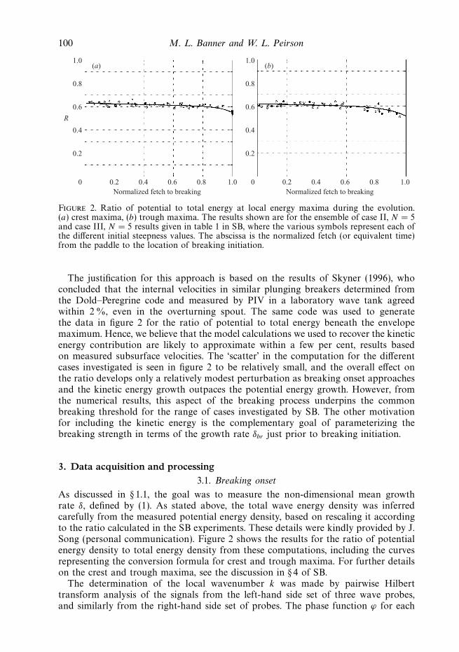
Figure 2. Ratio of potential to total energy at local energy maxima during the evolution.(a) crest maxima, (b) trough maxima. The results shown are for the ensemble of case II, N = 5and case III, N = 5 results given in table 1 in SB, where the various symbols represent each ofthe different initial steepness values. The abscissa is the normalized fetch (or equivalent time)from the paddle to the location of breaking initiation.

The justification for this approach is based on the results of Skyner (1996), whoconcluded that the internal velocities in similar plunging breakers determined fromthe Dold–Peregrine code and measured by PIV in a laboratory wave tank agreedwithin 2 %, even in the overturning spout. The same code was used to generatethe data in figure 2 for the ratio of potential to total energy beneath the envelopemaximum. Hence, we believe that the model calculations we used to recover the kineticenergy contribution are likely to approximate within a few per cent, results basedon measured subsurface velocities. The ‘scatter’ in the computation for the differentcases investigated is seen in figure 2 to be relatively small, and the overall effect onthe ratio develops only a relatively modest perturbation as breaking onset approachesand the kinetic energy growth outpaces the potential energy growth. However, fromthe numerical results, this aspect of the breaking process underpins the commonbreaking threshold for the range of cases investigated by SB. The other motivationfor including the kinetic energy is the complementary goal of parameterizing thebreaking strength in terms of the growth rate δbr just prior to breaking initiation.

3. Data acquisition and processing3.1. Breaking onset

As discussed in § 1.1, the goal was to measure the non-dimensional mean growthrate δ, defined by (1). As stated above, the total wave energy density was inferredcarefully from the measured potential energy density, based on rescaling it accordingto the ratio calculated in the SB experiments. These details were kindly provided by J.Song (personal communication). Figure 2 shows the results for the ratio of potentialenergy density to total energy density from these computations, including the curvesrepresenting the conversion formula for crest and trough maxima. For further detailson the crest and trough maxima, see the discussion in § 4 of SB.

The determination of the local wavenumber k was made by pairwise Hilberttransform analysis of the signals from the left-hand side set of three wave probes,and similarly from the right-hand side set of probes. The phase function ϕ for each


60(i)

(ii)

(iii)

(i)

(ii)

(iv)

40

2010 20 30 40

108610 20 30 40

0.2

0.1

010 20 30 40

20

–210 20 30 40

ηm

axµ

(t)

and

�µ

(t)�

µ(t

) an

d �µ

(t)�

δ(t

) ×

103

δ(t

)

k max

(rad

m–1

)

0.15

0.10

0.05

010 20 30 40

100 20 30 40–2

–1

0

1

2(× 103)

t/T t/T

µ(t)�µ(t)�

(a) (b)(m

m)

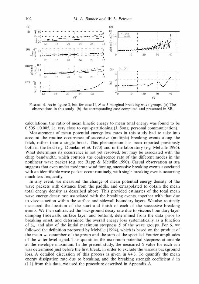
Figure 3. (a) Measured evolution properties with fetch, transformed to t/T , for the maximumrecurrence case II, N = 5 wave groups. (i) Carrier wave height at crest maxima (upper curve)and trough maxima (lower curve). (ii) Corresponding local wavenumber, smoothed as describedin the text. (iii) Corresponding evolution of µ(t) = Ek2 using the group velocity, with crestmaxima (upper curve) and trough maxima (lower curve). The central curve is the mean 〈µ(t)〉of the upper and lower curves. (iv) Non-dimensional mean growth rate δ(t), the normalizedderivative of µ(t), representing the convergence rate of wave energy to the envelope maximum.(b) the corresponding case computed in SB. (i) µ(t) and 〈µ(t)〉, (ii) The corresponding δ(t).

probe was computed and k determined from any pair of streamwise probes from therelationship k = ∂ϕ/∂x, using the measured phase difference and separation betweenthe two probes. With the ‘satellite’ probes located approximately 80 mm upstreamand downstream of the central probes, reliable estimates of the local wavenumberand the local variability could be obtained. The local wavenumber estimated in SBinvolved low-pass filtering the k distribution along the wave group, with the goal ofmatching the filtered k-value with the local zero-crossing analysis wavenumber. SBdiscusses this briefly, but Banner & Tian (1998, § 2.3.4), describes this in greater detail.In the present observational study, we followed the same approach, except that thelow-pass filtering was done in the time domain. The-low pass cutoff was set to providekmax values in the range 1 <kmax/klin < 1.3, as determined in Banner & Tian (1998)and SB. Here, klin is the nominal mean wavenumber determined from ωc using thelinear deep-water gravity wave dispersion relation. Results for the variation of thelocal wavenumber following the envelope maximum are shown for the case II, N =5maximum recurrence wave group case in figure 3, and for the marginal breaking casein figure 4. These figures also allow a detailed comparison to be made of the resultingtotal wave energy density with the SB computational results.

These figures confirm that our observational procedure was robust. The detailedresults are discussed in § 4, which also presents and discusses the full set of results forthe various initial wave steepness cases investigated.

3.2. Post-breaking energy losses and loss rates

The mean total wave energy 〈E〉 averaged over a wave group has been chosen asthe basis for quantifying the mean breaking energy loss and associated loss rate. Toconstruct the mean total energy from the mean potential energy measured in thisstudy, we again drew on the results of numerical computations in SB. From those


60(i)

(a) (b)

(ii)

(iii)

(i)

(ii)

(iv)

40

2012 20 2416 28 32

12 20 2416 28 32

12 20 2416 28 32

12 20 2416 28

12

8

0.2

0.1

0

321

ηm

ax (

mm

)µ

(t)

and

�µ

(t)�

µ(t

) an

d �µ

(t)�

δ(t

) ×

103

δ(t

)

k max

(rad

m–1

)0.2

0.1

0 10 20 30 40

100 20 30 40–2

0

2

4

(× 103)

t/T t/T

µ(t)�µ(t)�

Figure 4. As in figure 3, but for case II, N = 5 marginal breaking wave groups. (a) Theobservations in this study; (b) the corresponding case computed and presented in SB.

calculations, the ratio of mean kinetic energy to mean total energy was found to be0.505 ± 0.005, i.e. very close to equi-partitioning (J. Song, personal communication).

Measurement of mean potential energy loss rates in this study had to take intoaccount the routine occurrence of successive (multiple) breaking events along thefetch, rather than a single break. This phenomenon has been reported previouslyboth in the field (e.g. Donelan et al. 1973) and in the laboratory (e.g. Melville 1996).What determines its occurrence is not yet resolved, but may be associated with thechirp bandwidth, which controls the coalescence rate of the different modes in thenonlinear wave packet (e.g. see Rapp & Melville 1990). Casual observation at seasuggests that even under moderate wind forcing, successive breaking events associatedwith an identifiable wave packet occur routinely, with single breaking events occurringmuch less frequently.

In any event, we measured the change of mean potential energy density of thewave packets with distance from the paddle, and extrapolated to obtain the meantotal energy density as described above. This provided estimates of the total meanwave energy decay rate associated with the breaking events, together with that dueto viscous action within the surface and sidewall boundary-layers. We also routinelymeasured the location of the start and finish of each of the successive breakingevents. We then subtracted the background decay rate due to viscous boundary-layerdamping (sidewalls, surface layer and bottom), determined from the data prior tobreaking onset, and determined the overall energy loss systematically as a functionof δbr and also of the initial maximum steepness S of the wave groups. For S, wefollowed the definition proposed by Melville (1994), which is based on the product ofthe mean wavenumber of the group and the sum of the specified Fourier amplitudesof the water level signal. This quantifies the maximum potential steepness attainableat the envelope maximum. In the present study, the measured S value for each runwas determined just before the first break, in order to exclude the viscous backgroundloss. A detailed discussion of this process is given in § 4.3. To quantify the meanenergy dissipation rate due to breaking, and the breaking strength coefficient b in(1.1) from this data, we used the procedure described in Appendix A.


0.2(i)

(a)

(ii)

0.1

0 10 20 30 40 50

0.12 0.16 0.20 0.24

0.0100.0080.0060.0040.002

0

0.2(i)

(b)

(ii)

0.1

0 10 20 30 40 50

0.16 0.20 0.24

0.0100.0080.0060.0040.002

0

δbr

�µ (

t)�

S S

t/T t/T

5′ 4′ 3′ 2′1′

5 4 32

1

Figure 5. (a) Composite of the observed evolution curves for the mean energy 〈µ〉 for differentinitial maximum steepness levels S of case II, N = 5 wave groups (i) and their correspondinggrowth rates δbr just before breaking inception (ii). The identifiers 1′–5′ indicate increasingorder of S (b) corresponding computed results as presented in figure 12 of SB, withidentifiers1–5 indicating increasing order of S. Owing to the differential frictional attenuation betweenthe cases, the values of S in the experiments were measured just before breaking onset. Thelowest S value in (ii) corresponds to the maximum recurrence case, with its maximum growthrate.

4. Results4.1. Evolution properties

Figures 3(a)(i) and (ii) and 4(a)(i) and (ii) show the measured evolution behaviourof the wave elevation and the local wavenumber at the successive group crest andtrough maxima. Figure 3 shows the maximum recurrence case and figure 4 showsthe marginal breaking case, obtained by increasing incrementally the initial meancarrier wave steepness until breaking initiation was evident visually. Figures 3(a)(iii)and 4(a)(iii) show the corresponding evolution of µ at these maxima and minima,and also the calculated evolution of its average value, 〈µ〉, after smoothing out thefluctuations due to the crest and trough maxima, calculated from the average of thesmoothed spline fits to the crest and trough maxima. This follows the methodologydescribed in detail in Appendix B of SB. Figures 3(a)(iv) and 4(a)(iv) show thecalculated non-dimensional growth rate δ, which reflects the mean convergence rateof energy to (or from) the group maximum.

The major points of comparison are the non-dimensional energy µ values andnon-dimensional evolution times t/T (T is the mean carrier wave period), eitherat the recurrence maximum, or at the breaking onset time Tbr . It can be seen thatthe key values of the mean growth rate δ, either at the recurrence maximum or atbreaking onset, conform closely to the computed values. The recurrence cases havemaximum growth rates below the SB breaking threshold of (1.4 ± 0.1) × 10−3, whereasthe marginal breaking cases exceed this threshold close to breaking onset.

Figure 5(a) summarizes the ensemble of measured 〈µ〉 evolution curves as theinitial mean carrier wave steepness is increased for the case II, N = 5 wave groupsinvestigated. These are directly comparable with the upper panel in figure 12 ofSB, shown in figure 5(b). There is close correspondence between details of theobserved evolutional curves and model results. The non-dimensional time t/T toreach maximum recurrence is 42 in the model compared with 37 in the observations,


with a similar number of local crest and trough maxima. This close correspondencewas also found for the case II, N = 3 evolution results, with the non-dimensional timet/T to maximum recurrence of 24.0 in the observations compared with 23.4 in themodel, again with a similar number of local crest and trough maxima.

On the other hand, the modelled and observed evolutions for the case III wavegroups were significantly different, especially in terms of non-dimensional evolutiontime to maximum recurrence. As discussed in the last paragraph in § 2.2, we attri-bute this to the mismatch of initial wave-generation conditions in the model andexperiment. This was confirmed some time after these experiments were concludedwhen the flexible paddle had been replaced by a piston paddle to carry out a shallow-water study. A quick test using the ensemble of case II, N = 3 wave groups showedthe marginal break point shifted from 8.7 m for the flexible paddle to 14.3 m forthe piston paddle. Thus, a detailed quantitative comparison of the calculated andobserved evolution details with respect to t/T behaviour was not pursued for thecase III groups.

4.2. Breaking initiation threshold

One of the major aims of this study was to investigate, for a range of wave groupgeometries, the behaviour of the parametric energy convergence rate δ with increasingvalues of the initial carrier wave steepness, commencing with the marginal recurrenceevolution case. These results are shown in figures 3(a)(iv) and 4(a)(iv). These resultsshow that the maximum value attained by δ(t) for recurrence remains below thecommon breaking threshold value (1.4 ± 0.1) × 10−3 proposed by SB. Each of thesubsequent runs in which the initial mean carrier wave steepness (S) was increasedprogressively, such as is illustrated in figure 5(a), experienced breaking onset oncethat threshold level was exceeded, with a systematic decrease in both the time thatthe breaking threshold was first exceeded and the breaking onset time. These generictrends are evident for each of the wave group cases II and III investigated, andmirror the behaviour of the model calculations in SB. Table 1 summarizes the salientfeatures of each of the cases investigated in this study.

From their modelling study, SB noted that the proposed convergence-based break-ing criterion allows advance notice of breaking initiation. This was confirmed in thepresent set of observations. For example, in the case shown in figure 4, the breakingthreshold is exceeded at t/T ∼ 28, whereas breaking initiation occurs at t/T ∼ 32.The appropriate entries in table 1 show similar behaviour for each of the other casesobserved.

We made an assessment of the likely strength of viscosity effects on breakinginitiation. Following Tulin & Waseda (1999, § 3.2.3), the spatial amplitude decay rated(ln(a))/d(kx) for linear waves is dominated by the sidewall interaction and is givenby βD = (2ν/ω)/B , where a is the wave amplitude, x is the streamwise fetch, k and ω

are the wavenumber and frequency, ν is the kinematic viscosity of water and B is thetank width. For ν ∼ 10−6 m2 s−1 and B = 0.6 m, βD ∼ 8 × 10−4 and the correspondingenergy decay rate is βE ∼ 1.6 × 10−3. This translates into a loss of mean wave energyof about 20 %, or a reduction of about 2 mm in the wave amplitude (from 22 mm to20 mm) over the recurrence interval 10 < t/T < 47 in the wave tank.

To assess its significance on the measurements of parametric growth rates δ, βE

must be transformed to have the same growth rate form as δ = (1/ωc)(D〈µ〉/Dt),where µ = k2Eloc and Eloc is the depth-integrated potential plus kinetic energy. Thistransformation is straightforward and results in βE being reduced by the factor µ/π.Even for the largest value of µ ∼ 0.2, the transformed βE is 1.3 × 10−4, which is


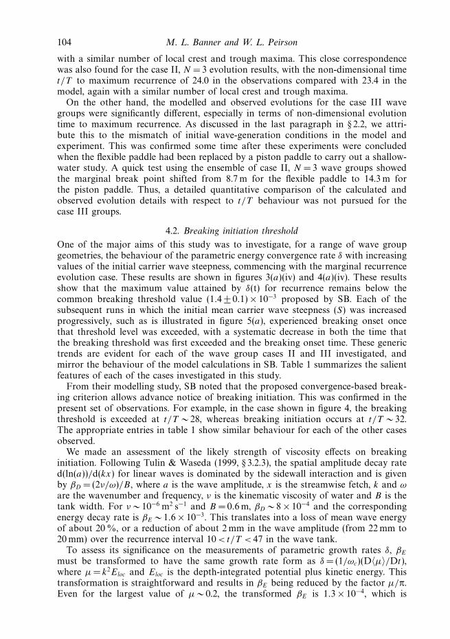
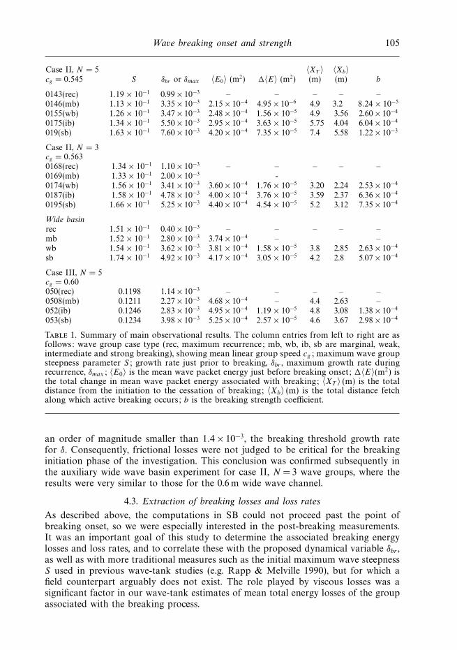
Case II, N = 5 〈XT 〉〈Xb〉cg = 0.545 S δbr or δmax 〈E0〉 (m2) �〈E〉 (m2) (m) (m) b

0143(rec) 1.19 × 10−1 0.99 × 10−3 – – – – –0146(mb) 1.13 × 10−1 3.35 × 10−3 2.15 × 10−4 4.95 × 10−6 4.9 3.2 8.24 × 10−5

0155(wb) 1.26 × 10−1 3.47 × 10−3 2.48 × 10−4 1.56 × 10−5 4.9 3.56 2.60 × 10−4

0175(ib) 1.34 × 10−1 5.50 × 10−3 2.95 × 10−4 3.63 × 10−5 5.75 4.04 6.04 × 10−4

019(sb) 1.63 × 10−1 7.60 × 10−3 4.20 × 10−4 7.35 × 10−5 7.4 5.58 1.22 × 10−3

Case II, N = 3cg = 0.5630168(rec) 1.34 × 10−1 1.10 × 10−3 – – – – –0169(mb) 1.33 × 10−1 2.00 × 10−3 -0174(wb) 1.56 × 10−1 3.41 × 10−3 3.60 × 10−4 1.76 × 10−5 3.20 2.24 2.53 × 10−4

0187(ib) 1.58 × 10−1 4.78 × 10−3 4.00 × 10−4 3.76 × 10−5 3.59 2.37 6.36 × 10−4

0195(sb) 1.66 × 10−1 5.25 × 10−3 4.40 × 10−4 4.54 × 10−5 5.2 3.12 7.35 × 10−4

Wide basinrec 1.51 × 10−1 0.40 × 10−3 – – – – –mb 1.52 × 10−1 2.80 × 10−3 3.74 × 10−4 – –wb 1.54 × 10−1 3.62 × 10−3 3.81 × 10−4 1.58 × 10−5 3.8 2.85 2.63 × 10−4

sb 1.74 × 10−1 4.92 × 10−3 4.17 × 10−4 3.05 × 10−5 4.2 2.8 5.07 × 10−4

Case III, N = 5cg = 0.60050(rec) 0.1198 1.14 × 10−3 – – – – –0508(mb) 0.1211 2.27 × 10−3 4.68 × 10−4 – 4.4 2.63 –052(ib) 0.1246 2.83 × 10−3 4.95 × 10−4 1.19 × 10−5 4.8 3.08 1.38 × 10−4

053(sb) 0.1234 3.98 × 10−3 5.25 × 10−4 2.57 × 10−5 4.6 3.67 2.98 × 10−4

Table 1. Summary of main observational results. The column entries from left to right are asfollows: wave group case type (rec, maximum recurrence; mb, wb, ib, sb are marginal, weak,intermediate and strong breaking), showing mean linear group speed cg; maximum wave groupsteepness parameter S; growth rate just prior to breaking, δbr , maximum growth rate duringrecurrence, δmax; 〈E0〉 is the mean wave packet energy just before breaking onset; �〈E〉(m2) isthe total change in mean wave packet energy associated with breaking; 〈XT 〉 (m) is the totaldistance from the initiation to the cessation of breaking; 〈Xb〉 (m) is the total distance fetchalong which active breaking occurs; b is the breaking strength coefficient.

an order of magnitude smaller than 1.4 × 10−3, the breaking threshold growth ratefor δ. Consequently, frictional losses were not judged to be critical for the breakinginitiation phase of the investigation. This conclusion was confirmed subsequently inthe auxiliary wide wave basin experiment for case II, N = 3 wave groups, where theresults were very similar to those for the 0.6 m wide wave channel.

4.3. Extraction of breaking losses and loss rates

As described above, the computations in SB could not proceed past the point ofbreaking onset, so we were especially interested in the post-breaking measurements.It was an important goal of this study to determine the associated breaking energylosses and loss rates, and to correlate these with the proposed dynamical variable δbr ,as well as with more traditional measures such as the initial maximum wave steepnessS used in previous wave-tank studies (e.g. Rapp & Melville 1990), but for which afield counterpart arguably does not exist. The role played by viscous losses was asignificant factor in our wave-tank estimates of mean total energy losses of the groupassociated with the breaking process.


0.25

0.20

0.15

0.10

0.050 10 20 30 40 50

�E�

(×

10–3

m2 )

t/T

∆�E�

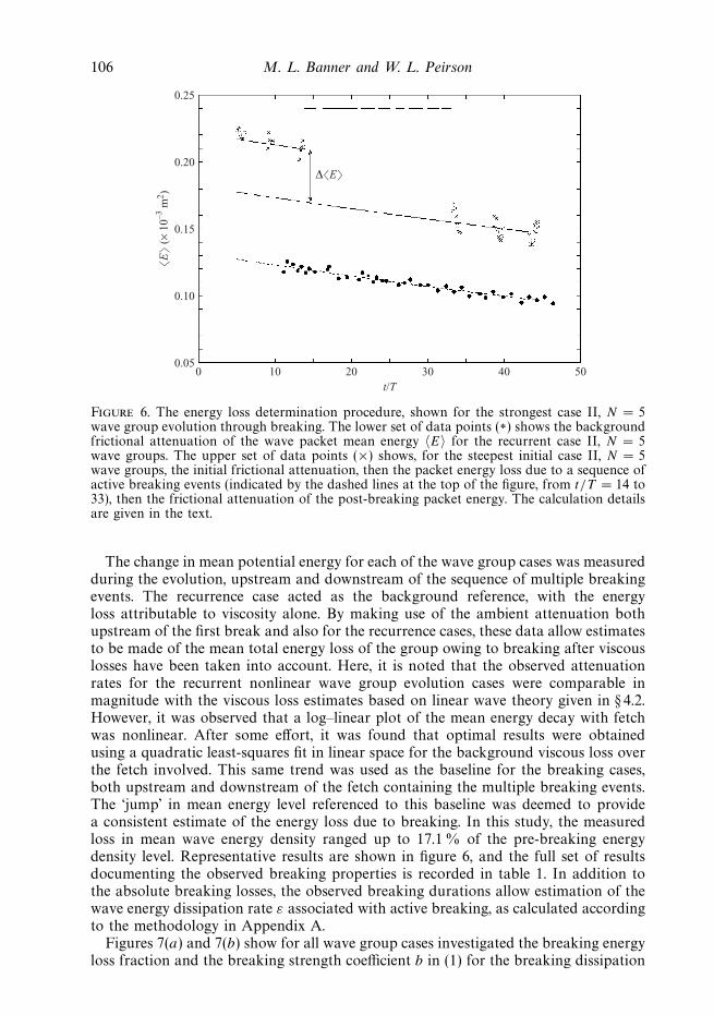
Figure 6. The energy loss determination procedure, shown for the strongest case II, N = 5wave group evolution through breaking. The lower set of data points (∗) shows the backgroundfrictional attenuation of the wave packet mean energy 〈E〉 for the recurrent case II, N = 5wave groups. The upper set of data points (×) shows, for the steepest initial case II, N = 5wave groups, the initial frictional attenuation, then the packet energy loss due to a sequence ofactive breaking events (indicated by the dashed lines at the top of the figure, from t/T = 14 to33), then the frictional attenuation of the post-breaking packet energy. The calculation detailsare given in the text.

The change in mean potential energy for each of the wave group cases was measuredduring the evolution, upstream and downstream of the sequence of multiple breakingevents. The recurrence case acted as the background reference, with the energyloss attributable to viscosity alone. By making use of the ambient attenuation bothupstream of the first break and also for the recurrence cases, these data allow estimatesto be made of the mean total energy loss of the group owing to breaking after viscouslosses have been taken into account. Here, it is noted that the observed attenuationrates for the recurrent nonlinear wave group evolution cases were comparable inmagnitude with the viscous loss estimates based on linear wave theory given in § 4.2.However, it was observed that a log–linear plot of the mean energy decay with fetchwas nonlinear. After some effort, it was found that optimal results were obtainedusing a quadratic least-squares fit in linear space for the background viscous loss overthe fetch involved. This same trend was used as the baseline for the breaking cases,both upstream and downstream of the fetch containing the multiple breaking events.The ‘jump’ in mean energy level referenced to this baseline was deemed to providea consistent estimate of the energy loss due to breaking. In this study, the measuredloss in mean wave energy density ranged up to 17.1 % of the pre-breaking energydensity level. Representative results are shown in figure 6, and the full set of resultsdocumenting the observed breaking properties is recorded in table 1. In addition tothe absolute breaking losses, the observed breaking durations allow estimation of thewave energy dissipation rate ε associated with active breaking, as calculated accordingto the methodology in Appendix A.

Figures 7(a) and 7(b) show for all wave group cases investigated the breaking energyloss fraction and the breaking strength coefficient b in (1) for the breaking dissipation


0.20(a) (b)

0.16

0.12

0.08

0.04

0 0.05 0.10 0.15 0.20

∆E—E0

case II, N = 3case II, N = 5case II, N = 3

2.0

1.6

1.2

0.8

0.4

0 0.05 0.10 0.15 0.250.20


b

(× 10–3)

S S

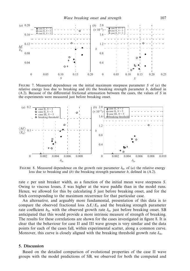
Figure 7. Measured dependence on the initial maximum steepness parameter S of (a) therelative energy loss due to breaking and (b) the breaking strength parameter b, defined in(A 2). Because of the differential frictional attenuation between the cases, the values of S inthe experiments were measured just before breaking onset.

0.2(a) (b)

0.1

0 0.002 0.004 0.006 0.008

�∆E�——�E0�

case II, N = 3case II, N = 5case III, N = 5breaking threshold

2.0

1.6

1.2

0.8

0.4

0 0.002 0.004 0.006 0.0100.008


b

(× 10–3)

δbr δbr

case II, N = 3case II, N = 5case III, N = 5breaking threshold

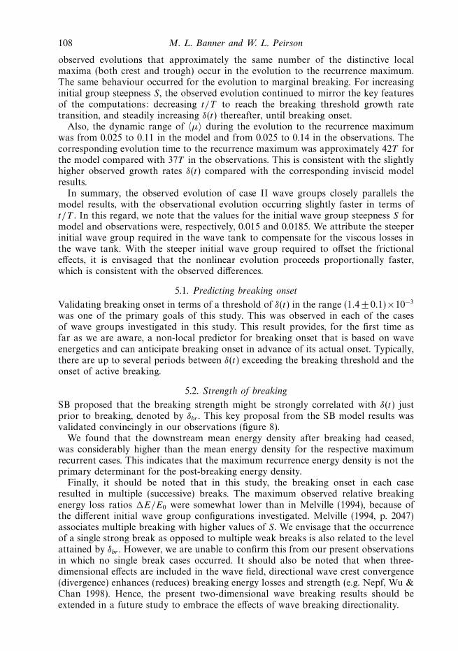
Figure 8. Measured dependence on the growth rate parameter δbr of (a) the relative energyloss due to breaking and (b) the breaking strength parameter b, defined in (A 2).

rate ε per unit breaker width, as a function of the initial mean wave steepness S.Owing to viscous losses, S was higher at the wave paddle than in the model runs.Hence, we allowed for this by calculating S just before breaking onset, and for thefetch corresponding to the maximum recurrence for that particular case.

An alternative, and arguably more fundamental, presentation of this data is tocompare the observed fractional loss �E/E0 and the breaking strength parameterrate coefficient bbr with the observed growth rate δbr just before breaking onset. SBanticipated that this would provide a more intrinsic measure of strength of breaking.The results for these correlations are shown for the cases investigated in figure 8. It isclear that the behaviour for case II and III wave groups is very similar and the datapoints for each of the cases fall, within experimental scatter, along a common curve.Moreover, this curve is closely aligned with the breaking threshold growth rate δth.

5. DiscussionBased on the detailed comparison of evolutional properties of the case II wave

groups with the model predictions of SB, we observed for both the computed and


observed evolutions that approximately the same number of the distinctive localmaxima (both crest and trough) occur in the evolution to the recurrence maximum.The same behaviour occurred for the evolution to marginal breaking. For increasinginitial group steepness S, the observed evolution continued to mirror the key featuresof the computations: decreasing t/T to reach the breaking threshold growth ratetransition, and steadily increasing δ(t) thereafter, until breaking onset.

Also, the dynamic range of 〈µ〉 during the evolution to the recurrence maximumwas from 0.025 to 0.11 in the model and from 0.025 to 0.14 in the observations. Thecorresponding evolution time to the recurrence maximum was approximately 42T forthe model compared with 37T in the observations. This is consistent with the slightlyhigher observed growth rates δ(t) compared with the corresponding inviscid modelresults.

In summary, the observed evolution of case II wave groups closely parallels themodel results, with the observational evolution occurring slightly faster in terms oft/T . In this regard, we note that the values for the initial wave group steepness S formodel and observations were, respectively, 0.015 and 0.0185. We attribute the steeperinitial wave group required in the wave tank to compensate for the viscous losses inthe wave tank. With the steeper initial wave group required to offset the frictionaleffects, it is envisaged that the nonlinear evolution proceeds proportionally faster,which is consistent with the observed differences.

5.1. Predicting breaking onset

Validating breaking onset in terms of a threshold of δ(t) in the range (1.4 ± 0.1)×10−3

was one of the primary goals of this study. This was observed in each of the casesof wave groups investigated in this study. This result provides, for the first time asfar as we are aware, a non-local predictor for breaking onset that is based on waveenergetics and can anticipate breaking onset in advance of its actual onset. Typically,there are up to several periods between δ(t) exceeding the breaking threshold and theonset of active breaking.

5.2. Strength of breaking

SB proposed that the breaking strength might be strongly correlated with δ(t) justprior to breaking, denoted by δbr . This key proposal from the SB model results wasvalidated convincingly in our observations (figure 8).

We found that the downstream mean energy density after breaking had ceased,was considerably higher than the mean energy density for the respective maximumrecurrent cases. This indicates that the maximum recurrence energy density is not theprimary determinant for the post-breaking energy density.

Finally, it should be noted that in this study, the breaking onset in each caseresulted in multiple (successive) breaks. The maximum observed relative breakingenergy loss ratios �E/E0 were somewhat lower than in Melville (1994), because ofthe different initial wave group configurations investigated. Melville (1994, p. 2047)associates multiple breaking with higher values of S. We envisage that the occurrenceof a single strong break as opposed to multiple weak breaks is also related to the levelattained by δbr . However, we are unable to confirm this from our present observationsin which no single break cases occurred. It should also be noted that when three-dimensional effects are included in the wave field, directional wave crest convergence(divergence) enhances (reduces) breaking energy losses and strength (e.g. Nepf, Wu &Chan 1998). Hence, the present two-dimensional wave breaking results should beextended in a future study to embrace the effects of wave breaking directionality.


5.3. Comparison with available field observations

In this study, the breaking strength coefficient has been defined in relation to the linearwave speed c, as in (A 2), rather than the actual breaker crest speeds cbr that havebeen used to date. This breaker strength coefficient is designated b, in contrast to bbr

defined in (2). The underlying motivation is related to self-consistent transformation,as discussed in detail in Appendix A § A 2. For the breaking waves in this laboratorystudy, we found values of b ranging between 8×10−5 and 1.2×10−3, with a near-lineardependence on the convergence rate parameter δbr . Since cbr ∼ (0.8–0.9)c, it is easilyseen that b ∼ O[(0.85)5] bbr ∼ 0.5bbr .

From their analysis of radar field data, Phillips et al. (2001) reported bbr ∼ (0.7–1.3) × 10−3. Allowing for the O(0.5) factor quoted in the previous paragraph, theselevels are comparable with those found in our laboratory study. On the other hand,Melville & Matusov (2002) quote a representative value of bbr ∼ 8 × 10−3 whichappears to have been inferred from laboratory data estimates of bbr in the range(3–16) × 10−3 (Melville 1994). After rescaling by 0.5 (see discussion at the end ofprevious paragraph), these values are about an order of magnitude higher than werefound for the spilling breakers in the present study.

In any event, for two-dimensional wave groups, we have observed a strongdependence of b on the rate of energy convergence and geometrical steepeningjust prior to breaking. In the field, breaking occurs in more complex wave groupsystems, and over a wide range of wave scales (e.g. as measured by their speed c),with potentially different convergence rates. Determining whether other parametersshould be included to more accurately characterize b remains to be explored in futurestudies.

5.4. Comparison of the present modulational growth rates and dissipation rates withother air–sea interaction growth rates

It is of interest to compare the characteristic mean growth rates and breaking lossrates observed in this study with characteristic growth rates in the closely relatedproblem of wind–wave generation. Banner & Song (2002) found that the impact ofwind forcing was secondary compared to hydrodynamic wave group evolution effects,even for relatively strongly forced cases. Hence, the unforced results are assumed to berepresentative of the wind-driven case, and will be used in the following comparison.

From the discussion in § 1.1, we recall that the definition of δ = (1/ωc)(D〈µ〉/Dt),where µ = Ek2, differs from the usual non-dimensional relative growth rate(1/ωcE)(DE/Dt). From our measurements, the latter is found to be O(0.05–0.10). Thiswas inferred using a similar procedure to that described in § 4.2, using typical values ofthe variables shown in the figures. Also, the observed dissipation rate associated withthe active periods of the multiple weak spilling breaking events in our experimentswas found to be O(0.005). In comparison, for the wind-driven problem, Donelan(1999) reported relative growth rates due to wind input ranging up to O(0.01) forvery strong generating conditions (typically the wind speed was seven times largerthan the wave speed), with a dissipation rate due to breaking of the same order ofmagnitude. Hence, it is seen that if the mean wave steepness is O(0.1), the group-mediated hydrodynamic energy fluxes can make a relatively strong contribution onthe short time scale. However, while local wave group modulation is believed to beoperative generally, it is tacitly assumed in spectral wind wave evolution models thatits net influence averages to zero over longer times. On the other hand, wave breaking,including the group-mediated contribution, is thought to be the major contributor tothe dissipation rate source term that describes the spectral mean loss rate of wave


energy. This term should also include a background wave energy loss rate associatedwith turbulence in the wave boundary-layer region. However, at present there is alack of consensus on the form of this term.

Given that spectral wave models do not resolve wave groups explicitly, the task ofincluding the above contributions is a significant challenge. Alves & Banner (2003)attempted to encapsulate the breaking contribution parametrically in a spectraldissipation source term premised on a breaking threshold that uses the spectralsaturation as a surrogate for δ. This choice was motivated by the relationship betweenthe spectral saturation, integrated over a logarithmic wavenumber bandwidth, andthe corresponding mean wave steepness, a classical measure of wave nonlinearity.Notwithstanding certain conceptual issues, the use of the spectral saturation as aviable breaking threshold parameter was investigated in detail in ocean storm wavemeasurements by Banner, Gemmrich & Farmer (2002). Others such as Badulin et al.(2005), have proposed substantially different perspectives on the nature and spectralrepresentation of wave dissipation. However, resolving this issue is well beyond thescope of the present contribution.

6. ConclusionsThe major conclusions of this investigation for wave breaking onset are as follows.(i) For both breaking and recurrence, the depth-integrated local energy density

following the maximum of the wave group was observed to evolve in a complexfashion, with a ‘fast’ oscillation superimposed on a longer-term mean trend. Thisbehaviour closely parallels the computational results reported in SB. In relation tobreaking onset, the ‘fast’ oscillation, due to the strong crest/trough asymmetry ofthe carrier waves, is believed to be primarily a kinematic effect. A non-dimensionalparametric growth rate δ(t) was derived from the mean trend of the diagnosticparameter µ(t), which reflects the systematic mean wave energy convergence andcarrier wave steepening towards the maximum energy region within the wave group.This growth rate appears to determine the ultimate breaking or recurrence behaviour.

(ii) Our measurements support the findings of the SB calculations that breakingor recurrence for two-dimensional chirped or unstable sideband deep water wavegroups are determined by a common growth rate threshold δth that is independentof the initial wave group structure. The numerical study of SB found that δth layin the range (1.4 ± 0.1) × 10−3. For the cases investigated in this study, recurrencebehaviour occurred for a maximum value of δ(t) that lies below this threshold, anddecreased thereafter. This is in contrast with the breaking cases investigated, whereδ(t) continued to increase after it reached this threshold level, after which breakingoccurred within a time interval ranging up to several carrier wave periods. Thus,using the growth rate δ provides an advance warning time of imminent breaking ofup to several carrier wave periods prior to breaking onset. To our knowledge, this isunmatched by any previously proposed breaking onset predictor.

The major conclusions of this investigation for wave breaking strength are asfollows.

(iii) The strength of breaking events is strongly correlated with the mean rateof convergence of energy and carrier wave steepening at the group maximumimmediately preceding breaking onset, as reflected by δbr , the corresponding value ofδ(t) just preceding breaking onset. For the two classes of wave groups investigated,an excellent collapse of the data was found between δbr and the breaking-induced


fractional energy loss, with significantly less scatter than for correlations based oninitial wave packet steepness.

(iv) The post-breaking mean energy density was found to remain significantlyabove the maximum energy density for maximal recurrent wave groups, which havecomparable local geometric and energetic waveforms. This further reinforces thehypothesis that breaking is more closely linked to wave energy convergence ratesrather than absolute local wave energy levels.

(v) The breaking strength parameter b in equation (A 2) for the dissipation rateper unit breaker crest length was deduced from measurements of the post-breakingenergy loss process. The results from the different cases collapsed on a common trend.The breaking strength parameter b ranged from 8 × 10−5 to 1.2 × 10−3 and was foundto have a strong near-linear dependence on the growth rate parameter δbr .

(vi) This study provides encouraging initial observational support for the nonlinearwave-group mediated onset of breaking within two-dimensional nonlinear wavegroups. The relevance of this approach to breaking onset and strength for fieldwave groups, which includes three-dimensional effects that are known to occur in theopen ocean, remains to be investigated. Other related fundamental issues work tobe resolved in future include understanding what determines the frequently observedoccurrence of multiple successive breaking events in a wave group.

This study has significant implications for future wave observational research. Thepresent generation of spectral wind wave models does not explicitly incorporate wavegroup effects. Energy convergence rates within wave groups may be several timesstronger than the wind input. This was seen in the numerical study of Banner & Song(2002), but is also evident in recent field observations of maturing wind seas. Thesehave relatively weak wind forcing at the spectral peak, yet are sufficiently steep fornonlinear effects to produce breaking of the dominant waves (e.g. see the top left-handpanel in figure 3 in Gemmrich 2005). This study highlights the need to gather space–time information that embraces evolving wave groups in order to improve ourpresent knowledge of wave breaking. Such instrumentation capabilities are becomingavailable and should be able to provide new insight into these key processes.

The financial support of the Australian Research Council and a University of NewSouth Wales Gold Star award for this project is gratefully acknowledged, together withthe expert assistance of the workshop staff at the UNSW Water Research Laboratory.During the course of the project the technical assistance of Chris Adamantidis, AinslieFraser, Rowan Hudson, David Dack, Evan Watterson and Ian Coghlan with themeasurements, and of Dr. Jinbao Song and Russel Morison with the data analysis,was instrumental in the execution and success of this study. MLB also acknowledgesthe ongoing support from the US Office of Naval Research during this investigation.

Appendix A. Estimating the breaking strength parameter b

A.1. Background

Originally developed for quasi-steady breaking, Duncan (1981, 1983) introduced themean energy density dissipation rate per unit length of breaking crest εL:

εL = bbrρwc5br/g. (A 1)

The unknown coefficient bbr quantifies the breaking strength, cbr characterizes thespeed of the breaking wave and ρw is the water density. Phillips (1985) appliedthis form subsequently for transient breaking in a spectral context. There is a


complementary form for the momentum flux transferred by the breaker to thesubsurface flow that involves the fourth power of cbr .

Equation (A 1) is based on the mean rate of working of a breaker of cross-sectionalarea Ab and propagation speed cbr against the orbital motion of the underlying wave.In unsteady breaking, cbr and Ab are time-dependent, and further assumptions areinvoked. Ab is assumed to maintain a constant aspect ratio, i.e. proportionality to λ2,the square of the wavelength of the breaking wave; a dispersion relation is assumedbetween λ and cbr which allows Ab to be expressed in terms of cbr . The coefficient bbr

in (A 1) incorporates these unsteady aspects.Several authors have provided estimates for cbr in relation to the corresponding

linear wave speed c of the other less steep waves in the group. For their oceanwhitecap measurement analysis, Melville & Matusov (2002) adopted cbr = 0.80c,while for microscale breakers, Jessup & Phadnis (2005) reported cbr = γ c, where γ

varied over the range 0.22 <γ < 0.85, according to the analysis methodology andcases investigated. In the present study, measured values of cbr = (0.9 ± 0.05)c werefound (see Appendix B below). In this context, note that for wave packets about tobreak, the departure from the linear wave speed c can be associated with the unsteadynonlinear distortion of the maximal wave in the packet. The local wavelength andwave period of the breaking wave contract owing to the nonlinearity. The effect isseen in figure A 2(a) of SB.

A.2. Transformation properties

Note that the choice of cbr in (A 1) has certain associated implications that have notbeen considered previously. These arise in relation to using this parameterization ofthe impact on breaking-induced dissipation rates and momentum fluxes in spectralwave model applications.

The issue of the most appropriate form for (A 1) arises in the context of estimatingspectral energy dissipation rates and momentum impulse contributions from breakingwaves in the field (e.g. Melville & Matusov 2002; Gemmrich 2005). Typically, videoimagery of the sea surface allows extraction of the spectral density of mean breakingcrest length Λ as a function of the observed breaker speed cbr . However, the usualspectral wave description is expressed in terms of linear Fourier mode speed c (or theequivalent frequency or wavenumber given by the linear wave dispersion relation),and a difficulty arises with the transformation if (A 1) is based on a cbr dependence.

In essence, the total energy dissipation rate ε and momentum impulse I

contributions from breaking waves involve fifth and fourth moments, respectively, ofthe Λ distribution, i.e.

ε =

∫bg−1c5 Λ(c) dc, I =

∫bg−1c4 Λ(c) dc.

The breaker image sequence measurements deliver estimates of Λ(cbr ), whereas themodels use Λ(c). These two forms are readily transformed by requiring the totalintegrated crest length to be conserved, hence Λ(c) = Λ(cbr )dcbr/dc. Assuming thatcbr ∼ γ c (see Appendix B), this transformation is straightforward. Further, it can beseen that the energy and momentum fluxes transform consistently if they are basedon c, but this no longer holds if they are based on cbr . On this basis, we recommendadopting the form

εL = bρwc5/g, (A 2)

and the following data analysis for quantifying b from the wave tank data in thisstudy is based on this equation.


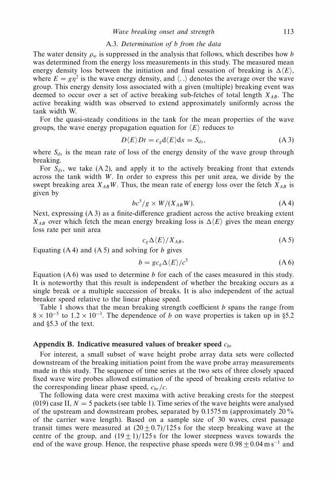
A.3. Determination of b from the data

The water density ρw is suppressed in the analysis that follows, which describes how b

was determined from the energy loss measurements in this study. The measured meanenergy density loss between the initiation and final cessation of breaking is �〈E〉,where E = gη2 is the wave energy density, and 〈. .〉 denotes the average over the wavegroup. This energy density loss associated with a given (multiple) breaking event wasdeemed to occur over a set of active breaking sub-fetches of total length XAB . Theactive breaking width was observed to extend approximately uniformly across thetank width W.

For the quasi-steady conditions in the tank for the mean properties of the wavegroups, the wave energy propagation equation for 〈E〉 reduces to

D〈E〉Dt = cgd〈E〉dx = Sds, (A 3)

where Sds is the mean rate of loss of the energy density of the wave group throughbreaking.

For Sds , we take (A 2), and apply it to the actively breaking front that extendsacross the tank width W . In order to express this per unit area, we divide by theswept breaking area XABW . Thus, the mean rate of energy loss over the fetch XAB isgiven by

bc5/g × W/(XABW ). (A 4)

Next, expressing (A 3) as a finite-difference gradient across the active breaking extentXAB over which fetch the mean energy breaking loss is �〈E〉 gives the mean energyloss rate per unit area

cg�〈E〉/XAB, (A 5)

Equating (A 4) and (A 5) and solving for b gives

b = gcg�〈E〉/c5 (A 6)

Equation (A 6) was used to determine b for each of the cases measured in this study.It is noteworthy that this result is independent of whether the breaking occurs as asingle break or a multiple succession of breaks. It is also independent of the actualbreaker speed relative to the linear phase speed.

Table 1 shows that the mean breaking strength coefficient b spans the range from8 × 10−5 to 1.2 × 10−3. The dependence of b on wave properties is taken up in §5.2and §5.3 of the text.

Appendix B. Indicative measured values of breaker speed cbr

For interest, a small subset of wave height probe array data sets were collecteddownstream of the breaking initiation point from the wave probe array measurementsmade in this study. The sequence of time series at the two sets of three closely spacedfixed wave wire probes allowed estimation of the speed of breaking crests relative tothe corresponding linear phase speed, cbr/c.

The following data were crest maxima with active breaking crests for the steepest(019) case II, N = 5 packets (see table 1). Time series of the wave heights were analysedof the upstream and downstream probes, separated by 0.1575 m (approximately 20 %of the carrier wave length). Based on a sample size of 30 waves, crest passagetransit times were measured at (20 ± 0.7)/125 s for the steep breaking wave at thecentre of the group, and (19 ± 1)/125 s for the lower steepness waves towards theend of the wave group. Hence, the respective phase speeds were 0.98 ± 0.04 m s−1 and


1.04 ± 0.55 m s−1. The latter is within the experimental scatter of the linear phase speedof 1.092 m s−1 whereas the former gives the estimate γ = cbr/c = 0.9 ± 0.04 based onthe paddle frequency, and within the noise of the observed wave speed. The observedreduction in breaker speed is appreciably less than that reported by Melville &Matusov (2002) and Jessup & Phadnis (2005).

REFERENCES

Alves, J. H. & Banner, M. L. 2003 Performance of a saturation-based dissipation source term forwind wave spectral modelling. J. Phys. Oceanogr. 33, 1274–1298.

Badulin, S. I., Pushkarev, A. N., Resio, D. & Zakharov, V. E. 2005 Self-similarity of wind drivenseas. Nonlinear Proc. Geophys. 12, 891–945.

Banner, M. L. & Peregrine, D. H. 1993 Wave breaking in deep water. Annu. Rev. Fluid Mech. 25,373–397.

Banner, M. L. & Song, J. 2002 On determining the onset and strength of breaking for deep waterwaves. Part 2: Influence of wind forcing and surface shear. J. Phys. Oceanogr. 32, 2559–2570.

Banner, M. L. & Tian, X. 1998 On the determination of the onset of breaking for modulatingsurface gravity water waves. J. Fluid Mech. 367, 107–137.

Banner, M. L., Gemmrich, J. R. & Farmer, D. M. 2002 Multiscale measurements of ocean wavebreaking probability. J. Phys. Oceanogr. 32, 3364–3375.

Dias, F. & Kharif, C. 1999 Nonlinear gravity and capillary-gravity waves. Annu. Rev. Fluid Mech.31, 301–346.

Dold, J. W. & Peregrine, D. H. 1986 Water–wave modulation. Proc. 20th Intl Conf. Coastal EngngTaipei, ASCE vol. 1, pp. 163–175.

Donelan, M. A. 1999 Wind-induced growth and attenuation of laboratory waves. In Wind overWave Couplings (ed. S. G. Sajjadi, N. H. Thomas & J. C. R. Hunt, Clarendon), pp. 183–194.

Donelan, M. A., Longuet-Higgins, M. S. & Turner, J. S. 1972 Whitecaps. Nature 239, 449–451.

Duncan, J. H. 1981 An experimental investigation of breaking waves produced by towed hydrofoil.Proc. R. Soc. Lond. A 377, 331–348.

Duncan, J. H. 1983 The breaking and non-breaking resistance of a two-dimensional hydrofoil.J. Fluid Mech. 126, 507–520.

Dysthe, K. B. 1979 Note on a modification to the nonlinear Schrodinger equation for applicationto deep water waves. Proc. R. Soc. Lond. A 369, 105–114.

Gemmrich, J. 2005 On the occurrence of wave breaking. Proc. Hawaiian Winter Workshop on RogueWaves (ed. P. Muller & D. Henderson), pp. 123–130. University of Hawaii SOEST.

Gemmrich, J. R. & Farmer, D. M. 2004 Observations of the scale and occurrence of breakingsurface waves. J. Phys. Oceanogr. 34, 1067–1086.

Holthuijsen, L. H. & Herbers, T. H. C. 1986 Statistics of breaking waves observed as whitecapsin the open sea. J. Phys. Oceanogr 16, 290–297.

Jessup, A. T. & Phadnis, K. R. 2005 Measurement of the geometric and kinematic properties ofmicrosacle breaking waves from infrared imagery using a PIV algorithm. Meas. Sci. Technol.16, 1961–1969.

Kway, J. H. L., Loh, Y.-S. & Chan, E.-S. 1998 Laboratory study of deep-water breaking waves.Ocean Engng 25, 657–676.

Loewen, M. R. & Melville, W. K. 1991 Microwave backscatter and acoustic radiation frombreaking waves. J. Fluid Mech. 224, 601–623.

Longuet-Higgins, M. S. 1984 Statistical properties of wave groups in a random sea state. Phil.Trans. R. Soc. Lond. A 312, 219–250.

Melville, W. K. 1982 The instability and breaking of deep-water waves. J. Fluid Mech. 115, 165–185.

Melville, W. K. 1983 Wave modulation and breakdown. J. Fluid Mech. 128, 489–506.

Melville, W. K. 1994 Energy dissipation by breaking waves. J. Phys. Oceanogr. 24, 2041–2049.

Melville, W. K. 1996 The role of surface-wave breaking in air-sea interaction. Annu. Rev. FluidMech. 26, 279–321.

Melville, W. K. & Matusov, P. 2002 Distribution of breaking waves at the ocean surface. Nature417, 58–63.


Nepf, H. M., Wu, C. H. & Chan, E. S. 1998 A comparison of two- and three-dimensional wavebreaking. J. Phys Oceanogr. 28, 1496–1510.

Osborne, A. R., Onorato, M. & Serio, M. 2000 The nonlinear dynamics of rogue waves and holesin deep water gravity wave trains. Phys. Lett. A 275, 386–393.

Papadimitrakis, Y. A., Huang, N. E., Bliven, L. F. & Long, S. R. 1988 An estimate of wavebreaking probability for deep water waves. In Sea Surface Sound – Natural Mechanisms ofSurface-Generated Noise in the Ocean (ed. B. R. Kerman), pp. 71–83. Kluwer.

Peirson, W. L. & Banner, M. L. 2000 On the strength of breaking of deep water waves. In CoastalEngineering 2000, ASCE, Sydney (ed. R. Cox), pp. 369–381.

Phillips, O. M. 1985 Spectral and statistical properties of the equilibrium range in wind-generatedgravity waves. J. Fluid Mech. 156, 505–531.

Phillips, O. M., Gu, D. & Donelan, M. A. 1993 Expected structure of extreme waves in a GaussianSea, Part 1. Theory and SWADE buoy measurements. J. Phys. Oceanogr. 23, 992–1000.

Phillips, O. M., Posner, F. L. & Hansen, J. P. 2001 High range resolution radar measurementsof the speed distribution of breaking events in wind-generated ocean waves: surface impulseand wave energy dissipation rates. J. Phys. Oceanogr. 31, 450–460.

Rapp, R. J. & Melville, W. K. 1990 Laboratory measurements of deep water breaking waves. Phil.Trans. Roy. Soc. Lond. A 331, 735–800.

Skyner, D. 1996 A comparison of numerical predictions and experimental measurements of theinternal kinematics in a deep-water plunging wave. J. Fluid Mech. 315, 51–64.

Song, J. & Banner, M. L. 2002 On determining the onset and strength of breaking for deep waterwaves. Part 1: Unforced irrotational wave groups. J. Phys. Oceanogr. 32, 2541–2558.

Stansell, P. A. & MacFarlane, C. 2002 Experimental investigation of wave breaking criteria basedon wave phase speeds. J. Phys. Oceanogr. 32, 1269–1283.

Terray, E. A., Donelan, M. A., Agrawal, Y. C., Drennan, W. M., Kahma, K. K., Williams, III,

A. J., Hwang, P. A. & Kitaigorodskii, S. A. 1996 Estimates of kinetic energy dissipationunder breaking waves. J. Phys. Oceanogr. 26, 792–807.

Thorpe, S. A. 1993 Energy loss by breaking waves. J. Phys. Oceanogr. 23, 2498–2502.

Tulin, M. P. & Li, J. J. 1992 On the breaking of energetic waves. Intl J. Offshore Polar Engng 2,46–53.

Tulin, M. P. & Waseda, T. 1999 Laboratory observations of wave group evolution, includingbreaking effects. J. Fluid Mech. 378, 197–232.

wave breaking onset and strength for two …ltalley/sio219/banner_peirson_jfm2007.pdf · wave...

Documents