water resources analysis of a multiobjective …
TRANSCRIPT
WATER RESOURCES ANALYSIS OF A MULTIOBJECTIVE DRAINAGE NETWORK IN THE INDIAN RIVER LAGOON BASIN
BY
DREW BURTON BENNETT
A THESIS PRESENTED TO THE GRADUATE SCHOOL OF THE UNIVERSITY OF FLORIDA IN
PARTIAL FULFILLMENT OF THE REQUIREMENTS FOR THE DEGREE OF MASTER OF SCIENCE
UNIVERSITY OF FLORIDA
1989

ACKNOWLEDGMENTS
My sincere thanks go to those individuals who provided
technical guidance, financial support, a "free-thinking"
work environment, and who interjected ideas and knowledge;
all of which contributed toward the completion of this
project. My time at the University of Florida and at the
Kennedy Space Center has led to an interaction with a wide
diversity of professionals, each addressing environmental
problems from a different perspective. This "melting pot"
arena has contributed immensely to my education.
Foremost, I would like to thank Professor James P.
Heaney, my committee chairman, for guidance, technical
expertise, and his encouragement to think. Thanks are also
due to Professor Wayne C. Huber and Dr. C. Ross Hinkle,
members of my committee, for their suggestions and review of
the manuscript. A large debt is owed to Mr. Robert E.
Dickinson of the Department of Environmental Engineering
Sciences at the University of Florida for his invaluable
assistance in understanding, applying, and modifying SWMM.
Funding for this research was provided by the National
Aeronautics and Space Administration through the Bionetics
Corporation of Kennedy Space Center, Florida, under contract
ii

number NAS10-10285. Dr. William M. Knott, III and Dr.
Albert M. Koller, Jr., of the NASA Biomedical Operations and
Research Office and Dr. C. Ross Hinkle of the Bionetics
Corporation are gratefully acknowledged for their support in
pursuing the issue and acquiring financial support for this
study.
Special recognition is given to Mr. Carlton Hall and Mr.
Mark Provancha, Bionetics Corporation, and Mr. Andreas
Goetzfried, EG&G Florida. These individuals have provided
time and encouragement and above all they provided valuable
insight into the water resources and environment of Merritt
Island, Florida.
A number of other individuals have been instrumental in
various aspects of the project and have provided literature,
data, discussion, and equipment. I acknowleqge Mr. Kirby
Key, Mr. Mario Busacca, and Mr. John Ryan of NASA; Dr. James
Kanipe, Mr. Harry Morton, and Ms. Rena Gaines of EG&G
Florida; and the Bionetics Ecological Programs staff.
Finally I wish to acknowledge my parents, Catherine and
Berkley Bennett, for their love, support, patience, and
sacrifice that enabled me to pursue an education.
iii


TABLE OF CONTENTS
ACIDiOWLEDGMENTS. . • . • . • • • . . • . • . . . • . . • • . . . . . . . . . . . . . . . ii
LIST OF TABLES...................................... vii
LIST OF FIGURES..................................... ix
ABSTRACT •••••••.•.•••••••••••••••••••••••••• e _ • • • • • • xii
CHAPTER I INTRODUCTION..................... 1
CHAPTER II DESCRIPTION OF STUDy............. 6
Description of Study Area. . . . . . . . . . . . . . . . . . . . . . . 6
Receiving Water Impacts......................... 14
Management Perspective.......................... 18
Methods/Approach. . . . . . . . . . . . . . . . . . . . . . . . . . . . . . . . 21
CHAPTER III STORMWATER MANAGEMENT OPTIONS FOR KENNEDY SPACE CENTER ........ . 23
Multiobjective Strategy.......................... 23
Selecting Management Options..................... 26
CHAPTER IV DATA COLLECTION AND SUMMATION .... 31
Precipitation. . . . . . . . . . . . . . . . . . . . . . . . . . . . . . . . . . . 31
Stage-Discharge Relationship.................... 33
iv

Groundwater Levels.............................. 40
Water Quality................................... 40
Total Suspended Solids..................... 43
Settleability of Runoff Pollutant Loadings. 44
Rating Curve for Total Suspended Solids Load •.•••...••.•...••..•..••••.•........ -. . 50
CHAPTER V HYDROLOGIC SIMULATION OF THE STUDY AREA....................... 56
Introduction ... '. . . . . . . . . . . . . . . . . . . . . . . . . . . . . . . . . 56
Goodness of Fit Criteria........................ 57
Runoff Block.................................... 59
Runoff Quantity Data Input................. 60
Calibration and Verification............... 67
Runoff Quality.................................. 73
Data Input................................. 74
Calibration. . . . . . . . . . . . . . . . . . . . . . . . . . . . . . . . 76
Estimates of Loadings from the Industrial Area Catchment. . . . . • • . . • . • . • • . • . . . . • • . . . . . . • • • . . . . . . 78
Data Input................................. 79
Resul ts. . . . . . . . . . . . . . . . . . . . . . . . . . . . . . . . . . . . 86
CHAPTER VI SIMULATION OF WATERSHED CONTROL SYSTEM PERFORMANCE •..••....•.•...
Preliminary Design for Demonstration Scale
94
Proj ect. . . . . . . . . . . . . . . . . . . . . . . . . . . . . . . . . . . . . . . . 97
Flood Control Performance.................. 98
Total Suspended Solids Removal Performance in Channel................................ 104
v

Groundwater Discharge to Channels.......... 109
other Performance Measures................. 110
Performance Measures specific to a Wetland System in Florida......................... 112
Performance Results............................. 114
Cost Analysis................................... 120
CHAPTER VII SUMMARY AND CONCLUSIONS •..••...•. 126
Summary. . . . . . . . . . . . . . . . . . . . . . . . . . . . . . . . . . . . . . . . 126
Conclusions .................................... 133
APPENDIX A
APPENDIX B
APPENDIX C
WATER LEVEL DATA BASE ASSEMBLED FOR THIS STUDy................... 138
LISTING OF SWMM INPUT FILES FOR THE STUDY AREA UNDER EXISTING LAND USE AND MAXIMUM BUILDOUT............. 139
DEVELOPMENT OF DISCHARGE COEFFICIENTS IN SWMM RUNOFF MODULE TO REPRESENT GROUNDWATER DISCHARGE AS A FUNCTION OF CHANNEL LENGTH................ 144
REFERENCES. • • • • • • • • • • • • • • • • • • • • • • . • • • . . . . . • • • • • • . • . • 145
BIOGRAPHICAL SKETCH................................. 154
vi


Table
II-1
III-1
III-2
III-3
IV-1
IV-2
IV-3
LIST OF TABLES
Page
Summary of Study Area Land Use at Kennedy Space Center.................................. 10
Multiobjective Analysis and Performance Measures for Comprehensive Stormwater Management Strategy........................... 24
Alternatives to Implement a Watershed Stormwater Management Strategy ...•............ 27
Decision Aid Matrix for Selecting Feasible Management Strategy for Detailed Analysis ..... 30
Stormwater Quality for the Vehicle Assembly Building Area of Kennedy Space Center for 1986 .......................... e • • • • • • • • • • • 42
Total Suspended Solids Loadings in Runoff from the study Area.................... . . . . . . . 45
Raw Total Suspended Solids Settleability Data. 52
V-I Runoff Block Parameters for Sub-Catchments 4 and 5....................................... 61
V-2 Runoff Block Water Quality Parameters ....•.•.. 75
V-3 Runoff Block Parameters for the Study Area. . . . . . . . . . . . . . . . . . . . . . . . . . . . . . . . . . . . . . . . . . 81
V-4 Calculations of Channel Buildup Length for Water Quality Simulation in RUNOFF ........ 84
V-5 Development Scenarios for the Industrial Area. . . . . . . . . . . . . . . . . . . . . . . . . . . . . . . . . . . . . . . . . . 85
V-6 Predicted Annual Loads to the Indian River Lagoon from the Study Area ...•..•.•........... 91
VI-1 Multiobjective Performance Measures for Watershed Control System .........•..•..•...... 96
vii

VI-2
VI-3
VI-4
VI-5
VI-6
VI-7
EXTRAN Junction Data for Standard Project Flood Analysis........................... . . . .. 106
Comparison of Untreated Drainage Water Quality with Wetland Drainage criteria .....•.. 115
Comparison of Performance for Existing System vs. Retrofitted System •••........•..•.. 116
Comparison of Performance for Existing Land Use and Maximum Buildout Specific to Florida Wetland Design Criteria .•......•.•. 119
Cost Analysis for Demonstration Scale Watershed Control System ••.••.•.••...•.••..•.. 123
Cost Analysis for Single Project Basins in a Subcatchment •..•...•........•..•......... 125
viii


Figure
11-1
11-2
11-3
11-4
IV-1
IV-2
IV-3
IV-4
IV-5
IV-6
IV-7
IV-8
IV-9
LIST OF FIGURES
Page
Location of the Study Area on Merritt Island, Florida.............................. 7
Brevard County Water Quality Planning Segments. . . . . . . . . . . . . . . . . . . . . . . . . . . . . . . . . . . . . 8
Study Area Subcatchments..................... 9
Yearly Mean Concentration of Selected Water Quality ~onstituents in Segment B2 of the Banana ~1 ver. . . . . . . . . . . . . . . . . . . . . . . . . . . . . . . . . 13
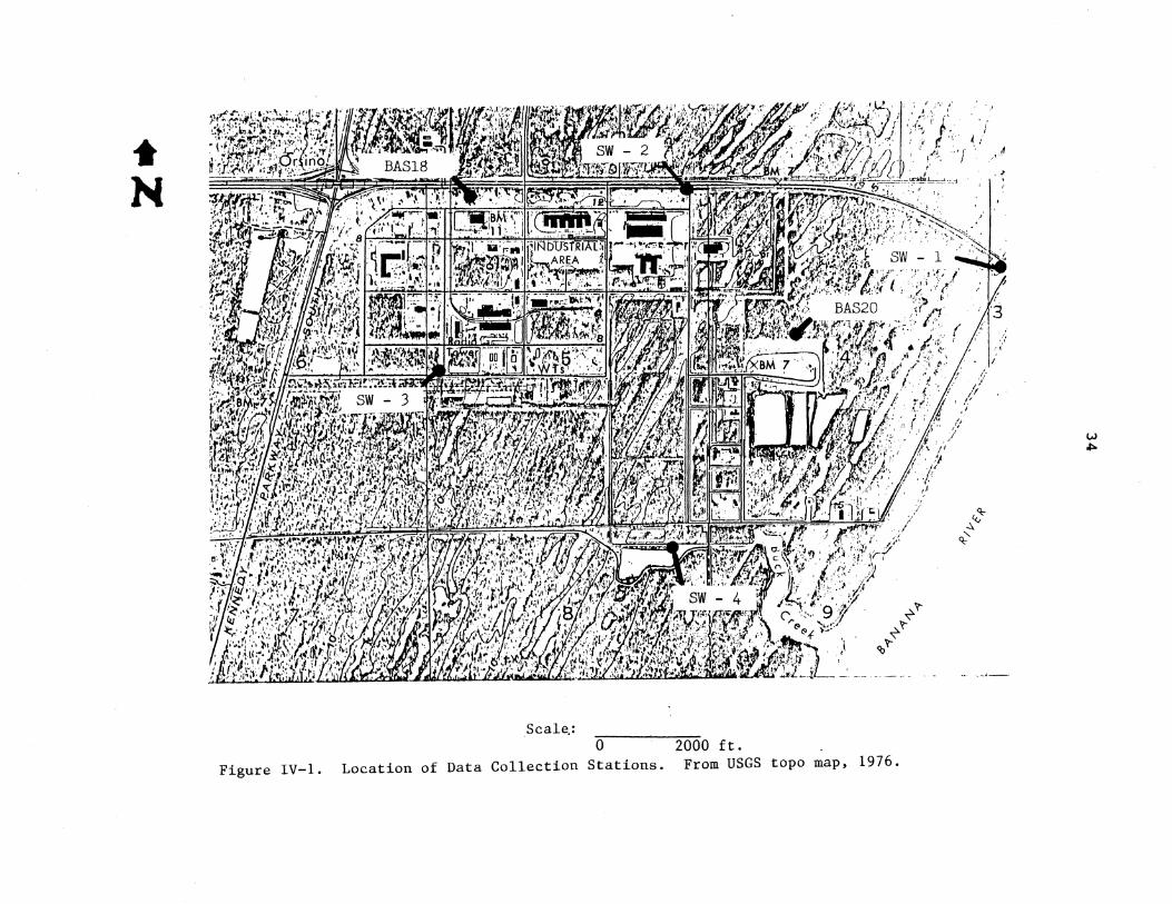
Location of Data Collection stations •...•..•• 34
Stage Data Collected at Station SW3 During the study Period............................. 38
Stage Data Collected at station SW2 During the study Period............................. 38
Stage-Discharge Rating Curve for station SW3. 39
Stage-Discharge Rating Curve for station SW2. 39
Groundwater Hydrographs for Observation Wells BAS 18 and BAS 2 0 . • • • . • . • . . • . . • . . . . . • . . • . • . • • • . 4 1
Results From the Differential Method for Reaction Order Determination as Applied to Total Suspended Solids Settleability in Kennedy Space Center Stormwater ...•..•..•..•. 49
Results of Settleability Tests for Total Suspended Solids in Kennedy Space Center Stormwater Effluent •.•••.••..•..••.••.••.•... 51
Simple Regression of Transformed Event Runoff Volume and Event Total Suspended Solids Load Data.................................... 54
ix

IV-10
V-1
V-2
V-3
V-4
V-5
V-6
V-7
V-8
V-9
V-10
V-11
V-12
V-13
Relationship Between Event Runoff Volume and Event Total Suspended Solids Load ....•....... 55
Peak Flow Results from the Calibration and Verification Runs--Catchment 4 ••......•...... 68
Total Flow Results from the Calibration and Verification Runs--Catchment 4 ............... 68
Peak Flow Results from the Calibration and Verification Runs--Catchment 5 •..•...•....... 69
Total Flow Results from the Calibration and Verification Runs--Catchment 5 ••...•.•••.•... 69
Measured and Predicted Hydrographs from a Calibration Run on Catchment 4. April 12, 1988 through June 15, 1988 .••....•...•..••... 70
Measured and Predicted Hydrographs from a Verification Run on Catchment 4. October 10, 1988 through November 2, 1988 •..•....•...•... 70
Measured and Predicted Hydrographs from a Calibration Run on Catchment 5. March 4, 1988 through March 7, 1988 ..•.•.•.....•...... 71
Measured and Predicted Hydrographs from a Verification Run on Catchment 5. October 10, 1988 through November 2, 1988 ...........•.... 71
Predicted and Measured Groundwater Table Elevation for Observation Well BAS18 in Catchment 4.................................. 72
Predicted and Measured Groundwater Table Elevation for Observation Well BAS20 in Catchment 5.................................. 72
Goodness of Fit of Event Total Suspended Solids Load.................................. 77
Schematic of the RUNOFF Simulation for the Entire study Area........................ . . . . 80
Predicted Annual Water Budget for the Study Area Under Existing Land Use Conditions ...... 87
x

V-14
V-15
V-16
V-17
V-18
VI-1
VI-2
VI-3
VI-4
VI-5
VI-6
Groundwater Discharge Under Existing Land Use in One Upland Subcatchment for a "Typical" year......................................... 88
Groundwater Discharge Under Existing Land Use in One Lowland Subcatchment for a "Typical" year................................ ..... .... 89
Combined "Typical" Year Discharge from the study Area under Existing Land Use .....•..... 90
"Typical" TSS Loads From the study Area Under Existing Land Use and the Maximum Buildout Development Scenarios •....••.....•.•..•...... 92
"Typical" Freshwater Runoff Volumes From the Study Area Under Existing Land Use and the Maximum Buildout Development Scenarios .•••... 92
Schematic Plan for the Proposed Demonstration Scale Watershed Control System •...•••..•••... 99
Schematic Comparison of the Existing Drainage Network and the Proposed Watershed Control System. . . . . . . . . . . . . . . . . . . . . . . . . . . . . . . . . . . . . .. 100
Schematic of EXTRAN Simulation for the Standard Project Flood Analysis •......•...... 105
Frequency of Mean Event Discharge for the "Typical" Year Under Varying Development Scenarios ..................................... 113
Frequency of Mean Event Discharge for NonControl and Watershed Control Under the Existing Land Use Scenario .•................. 121
Frequency of Mean Event Discharge for NonControl and Watershed Control Under the Maximum Buildout Scenario ...............•.... 121
xi


Abstract of Thesis Presented to the Graduate School of the University of Florida in Partial Fulfillment
of the Requirements for the Degree of Master of Science
WATER RESOURCES ANALYSIS OF A MULTI OBJECTIVE DRAINAGE NETWORK IN THE INDIAN RIVER LAGOON BASIN
By
Drew Burton Bennett
August 1989
Chairman: James P. Heaney Major Department: Environmental Engineering Sciences
The slow demise of the Indian River Lagoon in East-
Central Florida has been linked to drainage practices in
the Basin. The feasibility of implementing a watershed
control system at the Kennedy Space Center (KSC), Florida,
to meet multiple water management objectives is presented.
Site specific data were collected for the 1900 acre
Industrial Area catchment in KSC. These data were used to
calibrate and verify deterministic models of the watershed.
The U.S. Environmental Protection Agency's Storm Water
Management Model (SWMM) RUNOFF module was selected to
simUlate total runoff flow, peak flow, groundwater seepage
xii

to drainage channels, and storm event load of total
suspended solids (TSS). The relative effectiveness of
retrofitting the existing drainage network was evaluated
using other modules of SWMM including the storage/Treatment
Block and the EXTRAN Block. Both continuous simulation and
design storms were utilized in the analysis. Design
criteria for Standard Project Flood, TSS removal, reduction
in groundwater discharge, minimum and maximum water depths,
and mean event discharge were used to evaluate performance.
A watershed control system that includes constructing
weirs at channel outfalls with diversion of flow into
coastal wetlands was found to be relatively effective in
meeting many of the objectives. However, all the objectives
could not be met without making compromises in the
objectives. Due to analytical uncertainty, optimization of
the watershed control system without actual performance data
was not possible. Therefore, dynamic designs (i.e.
adjustable water control structures) are recommended.
Combining system performance data with dynamic simUlation
will allow fine tuning of the system. Study results suggest
that this aEproach provides an effective watershed control
strategy for the Indian River Lagoon Basin. Joint
research/application projects will be required in the future.
xiii


CHAPTER I
INTRODUCTION
Historically, control of stormwater has consisted of
collecting all runoff in gutters and discharging it into a
conveyance system of storm sewers and channels which are
tributary to a nearby stream, lake, estuary or ocean. A
hydraulically efficient urban drainage system implies the
use of storm sewers and lined and straight open channels.
In low lying areas of Florida, ditches were also constructed
to lower the groundwater table to improve the land for
development. Although these systems solved local flooding
problems, high peak flows and larger runoff volumes were
generated. In addition, these systems were found to have
little pollutant assimilative properties. An appreciation
of impacts of stormwater on natural systems and receiving
water bodies began to emerge in the early 1970's. Since
then, regulatory legislation on the control of environmental
impact from stormwater runoff has been evolving.
stormwater management has been a topic of extensive
study and debate over the last 20 years. Large amounts of
funds were spent in the 1970s and 1980s researching the
problem of non-point or diffuse pollution in stormwater
1

2
runoff on both the national and site specific scales. These
studies have made it possible to reasonably characterize
where this pollution originates, how it migrates through the
drainage network, and what technical solutions and
management strategies can be used to control it.
Unfortunately, much research in the stormwater area has been
limited to the small projects. This is largely the result
of funding agencies only wanting to focus on a single aspect
of this problem and to support applied research in their
narrowly targeted area.
After these findings and experiences, contemporary
stormwater management is undergoing transition and re
evaluation. The enormity of the control solutions and
regulatory enforcement is causing environmental managers to
re-examine current policies.
Depending on the regulatory program, contemporary
stormwater management includes efforts to control the
magnitude and frequency of floods and to reduce the severity
of water pollution events including erosion and
sedimentation problems. They are implemented through
standardized static designs which are based on idealized
representations of the hydrology and pollutant
characteristics. The operational procedures are fixed and
are not related directly to the system dynamics. This
approach is fostered by regulatory agencies who are faced
with the need to standardize the designs for ease of

3
enforcement since actual performance is not monitored.
Alternative technologies or operating procedures are not
readily accepted as they are generally required to include
extensive monitoring programs.
Over the past 5 years, Florida's Indian River Lagoon has
received national, regional, state, and local attention over
its degradation and the citizen's action and multi-agency
efforts to restore it. Degradation has included fish kills,
the reduction of viable recreational and commercial
fisheries, and loss of seagrass beds. Drainage practices on
the watershed have been identified as the primary culprit in
the slow demise of the Indian River Lagoon. specific
problems identified with the drainage are (1) the increase
in the volume of freshwater runoff, (2) the increase in the
deposition of organic sediments, (3) the reduction in water
clarity due to the increased discharge of "colored"
groundwater (a result of tannic acid) and suspended solids,
and (4) eutrophication due to nutrient loadings. Poor
flushing characteristics of lagoon segments intensify
impacts due to runoff. stricter stormwater regulations for
new development and retrofitting of existing drainage
systems within the Indian River Lagoon watershed are being
considered by agencies as potential control and mitigation
strategies. NASA's John F. Kennedy Space Center (KSC)
comprises approximately 7% of the Indian River Lagoon's
drainage basin and receiving waters surrounding KSC have
been designated outstanding Florida Waters by the State of

4
Florida. To aid NASA in meeting environmental commitments,
predictive capabilities of impact on the watershed scale are
being developed so that cost-effective mitigation strategies
can be initiated.
The goal of this project is to take a first step in
developing a watershed scale strategy towards managing
drainage and urban runoff from KSC. This project focuses on
analyses of data from the Industrial Area sub-catchment of
KSC which discharges to the Banana River portion of the
Indian River Lagoon. The principal objectives of this
project are
(1) collect site specific data representative of typical
KSC catchments for detailed analysis of viable options;
(2) develop a satisfactory methodology for estimating
freshwater and pollutant loads from upland drainage areas;
(3) identify feasible control alternatives;
(4) determine the feasibility of retrofitting existing
drainage networks from a multiobjective performance
standpoint;
(5) determine whether a watershed control system will
also satisfy new development requirements; and
(6) establish a water resources knowledge base for KSC.
Previous work in stormwater management, including
information on the study area and the study approach, are

5
discussed in Chapter II. Chapter III examines the water
management objectives, the options available to KSC for
stormwater management, environmental decision making, and
documents the selection of channel retrofitting with wetland
routing as the most feasible alternative. The methods for
data collection and analysis are summarized in Chapter IV.
Chapter V provides documentation of the calibration and
verification of SWMM for use in hydrologic simulation of the
study area. The runoff and total suspended solids loads for
the existing land use and the maximum buildout development
scenario are also presented. Chapter VI contains the
results of the proposed watershed control system performance
evaluation with respect to the multiple objectives. Chapter
VII summarizes the findings and offers conclusions.


CHAPTER II
DESCRIPTION OF STUDY
Description of Study Area
The Industrial Area of KSC was selected as a
representative catchment that is relatively developed and
continues to be developed. It consists of 1900 acres of
partially developed land set amongst undeveloped Florida
Flatwoods on Merritt Island, Florida (a remnant barrier
island). The study area, in relation to Merritt Island, is
shown in Figure II-1. Approximately 700 acres are managed
by the U.S. Fish and wildlife Service (USFWS) as part of the
Merritt Island National Wildlife Refuge (MINWR). Runoff
from the catchment drains to Segment B2 (as identified by
the Brevard County 208 study) of the Banana River (see
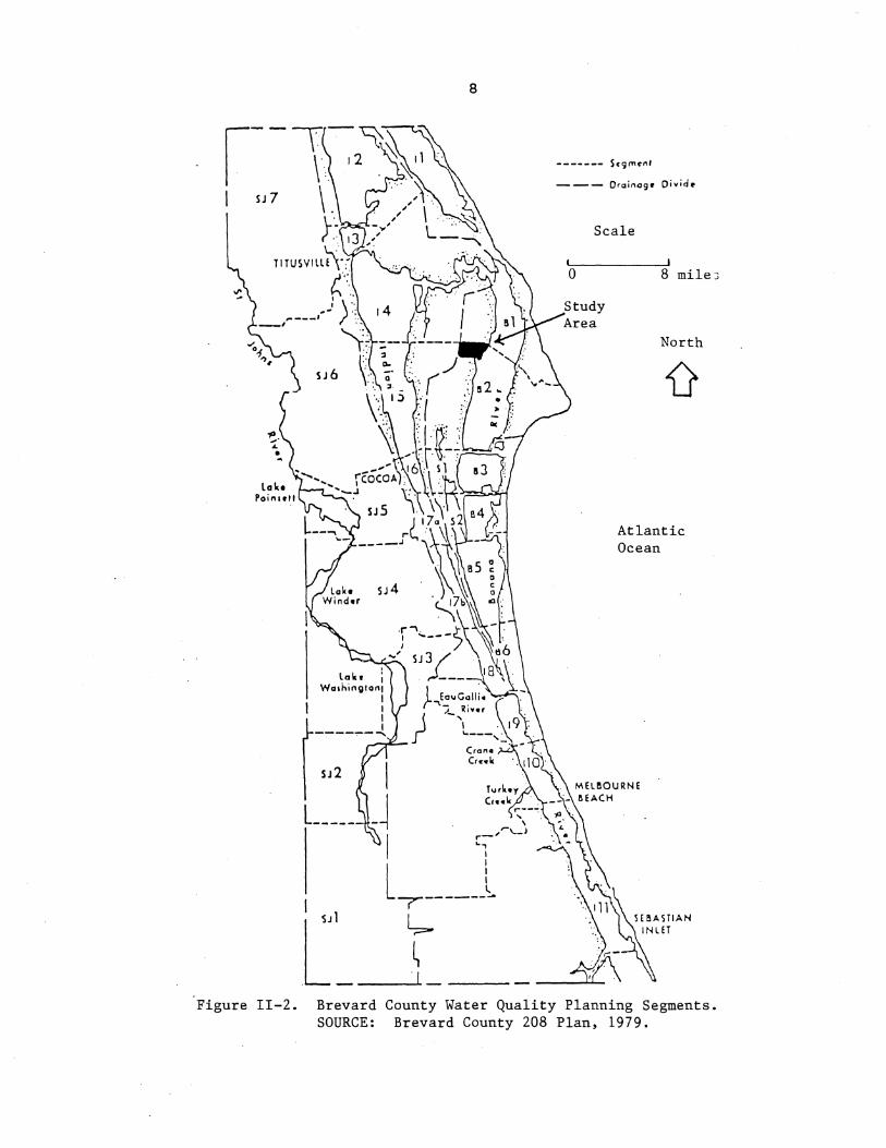
Figure II-2). The study area catchment can be divided into
six sub-catchments as delineated in Figure II-3. Land use
for the entire study area and by individual catchment is
summarized in Table II-1.
6

405
Indian River
Merritt Island
7
Banana River
SCALE IN FT.
~ o
15:300 ft0l
Atlantic Ocean
L-_____________________ --=-____ ._._ .. ___ -!.
Figure II-i. Location of the Study Area on Merritt Island, Florida. SOURCE: NASA, 1986.
8
------- Scgmen/
--- Orainage Oivid.
o
Scale
8 mile:;
North
Atlantic Ocean
Figure 11-2. Brevard County Water Quality Planning Segments. SOURCE: Brevard County 208 Plan, 1979.

Scale: I I o 2000 ft.
Figure 11-3. Study Area Subcatchments. From USGS topo map, 1976.
I,
I ~ .. i l
'" I.'
II
./ .,.,{ ./1 ./
~'?' ~'?'
CQ'?'
«-q" ~
~
J
\0

10
Table II-1. Summary of Study Area Land Use at KSC.
LAND USE
Undeveloped Undeveloped Ruderal Open Channels Impervious Total CATCHMENT Wetland Upland & Borrow Pits
1 Acres 23.7 514.5 0.0 39.0 0.0 577.2 % 4.1 89.1 0.0 6.8 0.0 100
3 Acres 95.0 233.1 64.2 34.4 63.1 489.8 % 19.4 47.6 13.1 7.0 12.9 100
4 Acres 0.1 7.7 71.1 9.7 78.5 167.1 % 0.1 4.6 42.5 5.8 47.0 100
5 Acres 0.0 33.1 38.5 0.0 61.2 132.8 % 0.0 24.9 29.0 0.0 46.1 100
15 Acres 0.0 0.0 123.0 0.0 95.5 218.5 % 0.0 0.0 56.3 0.0 43.7 100
24 Acres 46.8 179.2 26.0 19.0 44.6 315.6 % 14.8 56.8 8.2 6.0 14.1 100
Total Acres 165.6 934.5 284.3 102.1 281. 7 1901 % 8.7 49.2 15.0 5.4 14 .8 100
Ruderal: Vegetation disturbed by man (e.g. lawn, roads ides) .
Impervious: Roadways, rooftops, parking lots.
11
Geographical information for the study area was
generated by updating existing soil and vegetation map files
(Provancha et al. 1986) with cultural and urban features on
the ERDAS geographical information system. The added
features were digitized from KSC Master Planning maps at a
scale of 1:9600. ERDAS utilizes a raster format; the pixel
size for existing data files is 0.12 acres (73.79 ft. by
73.79 ft.).
As typical with most Florida Flatwood watersheds, the
undeveloped portions of the study area can be characterized
as having (1) extremely flat relief, (2) sandy soils, (3)
dynamic shallow water table, and (4) scattered wetlands,
locally referred to as interdunal swales. A very large
portion of the relief for the area is the result of an
extensive open channel drainage network constructed by the
U.S. Army Corps of Engineers (COE) in the 1960's. The
objective of the COE was to protect federal facilities from
flooding by improving drainage. The drainage system has
performed well (no flooding of .facilities has been reported)
and is continually maintained.
Buck Creek is a freshwater tributary to segment B2.
Improved drainage channels have also been connected with
Buck Creek. The remainder of the tributaries are man-made
open drainage channels. None of these tributaries have been
gauged for discharge in the past.

12
Segment B2 is approximately 16,000 acres in size, with a
length of 7 miles and a width of 3 miles. The average depth
is approximately 3.5 feet with the exception of barge
channels which have a design depth of 12 feet. It drains
approximately 31,000 acres of uplands from both Merritt
Island and Cape Canaveral. Approximately 1800 acres are
developed. The KSC Industrial Area accounts for 40% of this
development.
smith (1985) reports an astronomical tide elevation
range of less than 0.03 feet in this part of the Indian
River Lagoon. Changes in water level and current are due
primarily to freshwater runoff and aeolian tides. Smith et
al. (1987) used harmonic analyses of water level records
near Melbourne, Florida to quantify components of the tide.
They have shown that in the central part of the Indian River
Lagoon nontidal variance characteristically accounts for 40-
60% of the total. He notes that the non-tidal variation is
quasi-periodic at best, but suggests that relative maxima
occur approximately every five days as the result of a
variety of forms of meteorological forces. Mixing and
spreading of dissolved and suspended sUbstances in the
lagoon is a slow process; Carter and Okubo (1965) suggest a
residence time of 150 days.
Yearly mean concentrations (1980-1985) of salinity,
dissolved oxygen, total nitrogen, total phosphorous, and
chlorophyll-a for Segment B2 are reported in Figure II-4.

z 0
~ f--z w 0 z 0 0
13
32
30
28
26
24
22 ' .. ", ...
20 .............. 18
16
14
12
10
8
6 -.-.---.--.-.-.-.-.:.~.:.~.-.•. ~ =: - - - - - - -- - -+-- - - -- - - - - - - - - -+----- ----------+-- - - -- - - - - -----
4
2
---~---------------~---------------6----0·· .. '.. 0···
o 4----------,---------,----------,---------,---------~ 1980 1981 1982 1983
YEAR
Salinity (1000 mg/L)
DO (mg/L)
TN (mg/L)
TP (mg/L * 100)
Chlorophyll a (mg/L)
1984
Figure 11-4. Yearly Mean Concentration of Selected Water Quality Constituents in Segment B2 of the Banana River. SOURCE: Brevard County Department of Natural Resources (1987).
1985

14
Peffer (1975) found that the bulk of the bottom sediments in
the lagoon have a negative oxidation-reduction potential
(Eh) and consequently concluded that the sediments act as a
nutrient trap.
Four roles seagrass play in the ecology of an estuary
are (1) habitat, (2) food source, (3) nutrient buffer, and
(4) sediment trap. Among the major ecological values of
seagrass meadows is the fact that many recreationally and
commercially valuable fishery organisms utilize these
systems for part or all of their life history (Fonseca et
ale 1986). Seagrass and/or submerged aquatic vegetation
covers approximately 70% of Segment B2's bottom
(Provancha and Willard, 1986).
Receiving Water Impacts
The importance of the stormwater problem in terms of
direct and indirect impacts on receiving waters is now
receiving more attention. Heaney et ale (1979) stimulated
interest in direct assessment of receiving water impacts by
pointing out the very high cost of controlling runoff (an
initial estimate of $200 to $400 billion for the nation).
An early national inventory of available information on
receiving water impacts (Heaney et ale 1981) revealed
fundamental gaps in our knowledge. A more recent review,
specific to estuarine systems (Odum and Hawley, 1986), notes

15
that there are virtually no published studies which
definitively show degradation of a significant estuarine
area as a result of urban runoff. They go on to suggest
that this is due to (1) the tendency for urban runoff and
its effects to be interrelated with a host of other
pollutant sources and their effects, and (2) a lack of
recognition by estuarine scientists of the potential threat
from urban runoff pollution.
The EPA's Nationwide Urban Runoff Program (NURP)
sponsored several studies, including one in Tampa Bay, to
measure wet-weather impacts on receiving waters. The Tampa
Bay study revealed no acute toxicity to test organisms (Mote
Marine Laboratory, 1984). In contrast, Odum and Hawley
(1986) note that there is considerable circumstantial
evidence pointing to urban runoff as a serious pollution
source. They note examples along all coasts of the United
states, including the Chesapeake Estuary and Biscayne Bay,
in which damage from urban runoff is occurring but has not
been well documented. In all cases the impact of urban
runoff is masked by a variety of other pollutant inputs.
Obviously, the assessment of impact is an extremely
difficult task because (1) one must filter through numerous
environmental variables over which the researcher has no
control, (2) the definition of impact varies with the
individual and their personal values, and (3) the impact is
transient.

16
Perhaps the best synthesis of information on receiving
water impacts and degradation of the Indian River Lagoon is
found in steward and Van Arman (1987). Although a great
deal of data have been reviewed and synthesized, the
conclusions of this report are largely ancedotal and lack
data clearly documenting cause and effect relationships.
Steward and Van Arman (1987) point out three major impacts
on the Lagoon often associated with land drainage and
runoff: (1) eutrophication due to nutrient loadings, (2)
"muck" deposition, and (3) buildup of toxins and pathogens
in biota. Poor flushing characteristics of lagoon segments
intensify impacts due to runoff.
Turbidity is an expression of the optical quality of a
water sample to scatter and absorb light. The penetration
of light in water can be reduced by several factors
including algal blooms, suspended solids, and "colored"
water (tannic acid). Light penetration in estuaries
regulates the productivity of phytoplankton and seagrasses
(Rice et al. 1983; Heffernan and Gibson, 1983).
The roles of groundwater discharge in the lagoon ecology
are poorly understood. Drainage of uplands around the
lagoon has concentrated and increased flows from the
surficial aquifer, routed them to stormwater outfalls, and
altered the hydrology and constituent loads. Any benefits
of natural diffuse groundwater flows have likely been lost.
Thompson (1978) and Steward and Van Arman (1987) speculated

17
that reduced light levels due to point source discharges of
"colored" groundwaters were partially responsible for the
poor conditions of the seagrass beds. Materials responsible
for color in water exist primarily in colloidal suspension
and are not due to dissolved materials (Black and Christman,
1963).
In a study on muck in the Indian River Lagoon, Trefry et
ale (1987) found that the muck has been deposited over the
last 20 to 30 years and that the two sources which
contribute to the accumulation of muck are soil runoff and
organic matter (e.g. plant remains). Using Turkey Creek as
a field test site, Trefry et ale (1988) determined that
iron-rich inorganic minerals (e.g. clays) make up 50-80% of
the suspended sediment. Organic matter rich in nitrogen and
phosphorous adds 10-40% to the suspended load.
In a comprehensive report to NASA, Laster (1975)
reported that waters in the vicinity of KSC appear to be
experiencing some degree of degradation. He speculated that
nutrient materials derived from urban and agricultural
runoff were the cause rather than effluents derived from
"space oriented" activities. High concentrations of
nutrients were found to be accumulating in sediments near
the CCAFS sewage treatment plant outfall located 2.8 miles
from the study area outfalls.

18
Management Perspective
In the 1970's emphasis on environmental management was
based on risk aversion (strong anti-degradation philosophy) .
Due to the tremendous costs associated with the risk
aversion approach, environmental risk assessment is swinging
back to a cost-effective approach used in sanitary
engineering prior to the 1970's. The cost-benefit
reliability approach to stormwater and drainage problems is
by no means the only perspective, even today. During a 1984
workshop on contaminants in Florida's coastal zone (Delfino
et ale 1984), 200 scientists concluded that they could not
put the value of controlling contaminants in dollar terms.
They recommended that a procedure should be established to
accurately quantify ecological and esthetic values. To
date, no accepted interdisciplinary procedure has been
developed.
The goal of stormwater management is to reduce its
effects to an acceptable level, a compromise between costs
and benefits. It is impossible to predict costs and
benefits precisely. Predicting the effects of the
hydrologic changes (flow rates, water quality,
sedimentation) is complex and much less accurate than say
calculating peak runoff discharges. It is important not to
lose perspective that the concern is not over the quantity
of a specific chemical in water, but what effects the
chemical at a specific concentration will have on biota and

19
the subsequent benefit derived from the impacted water
resource.
Program-related standards specifying pollutant
concentrations and peak discharge ease implementation and
enforcement of regulations. However, Heaney (1988) pointed
out that this approach has been relatively ineffective given
the performance results of dry-weather wastewater treatment
plants under such an approach. Heaney noted that while it
is relatively easy to run computer models to tabulate the
statistics for a prescribed standard, it is an onerous
effort to develop the actual field and laboratory
information to support such a recommendation.
Increased environmental regulation has led to more
pollution abatement measures. Increasing costs of pollution
abatement services, construction, and monitoring have
resulted in environmental management funds taking a larger
percentage of available funds. Often this increased
spending has led to little perceived benefit. For the case
of stormwater regulation in Florida, performance standards
have been promulgated even though performance is rarely
monitored and the consequences of any violation are poorly
understood or documented.
The nation continues to struggle with a national
strategy for implementing stormwater programs to meet the
objectives of the Clean water Act. The Florida Department

20
of Environmental Regulation (FDER) developed a regulatory
program for the control of non-point sources. Livingston
(1986) summarizes The Stormwater Rule as having established
a performance standard for the treatment of stormwater. The
performance standard is based on two properties of
stormwater (1) annual storm frequency distribution, and (2)
the first flush of pollutants. The rule's basic objective
is to achieve 80-90% removal of stormwater pollutants before
discharge to receiving waters. Thousands of stormwater
basins have been designed and constructed to FDER
performance standards; yet very few have been monitored for
performance.
Livingston (1986) summarizes some of the major problem
areas with the Stormwater Rule. A number of them apply to
the KSC drainage network. The grand fathering of drainage
systems constructed prior to the Rule is one. The
retrofitting of existing systems that are causing water
quality degradation is a major objective of the stormwater
legislation. Little verification of removal effectiveness
of systems permitted and constructed under the Rule is
another. Recent performance evaluations of stormwater
detention/retention basins meeting The Stormwater Rule
specifications by Holler (1989) and Martin (1988), suggest
that the state's goal is not being met. Because of poor
retention system performance in flat, high water table areas
like KSC, an effective alternative is sought. wet detention
basins are now being considered for general permit

21
applications. Perhaps one of the most fundamental flaws
identified is the promotion of a piecemeal approach to
stormwater management which relies upon individual on-site
stormwater management. A potential problem with this
approach is the combined effects of individual randomly
located detention basins which can increase downstream peak
flow and cause channel scouring. The proliferation of
numerous small on-site systems increases the difficulty of
enforcing operation and maintenance requirements. The
agency is now promoting a watershed management approach.
In addition, the rule does not address other drainage
associated problems such as sediment scour in drainage
channels or the discharge of "colored" groundwater into the
drainage system.
Methods/Approach
Field documentation of impact, especially long-term
degradation, and effectiveness of control alternatives is
difficult, laborious, and costly. Even when the studies are
completed, the results are difficult to extrapolate to other
development scenarios. Mathematical models offer a quicker
and less costly approach to overall assessment of stormwater
runoff and drainage problems. Models are efficient
environmental quality management tools that are based on an
accumulation of knowledge of the environmental phenomena to

22
be managed; however, they are not intended to sUbstitute for
"real" data collection.
To minimize extensive and expensive field data
collection, it was felt that runoff, water routing, and
control can be reasonably predicted using existing models
such as EPA's storm water Management Model (Huber and
Dickinson, 1988). The requirements of the selected model
were to help organize and visualize cause and effect
relationships in the catchment and to assist in comparisons
of control alternatives. To lend credibility to the
predictions, local calibration/verification data were
collected. For planning and overall assessment, continuous
simulation (on the order of months or years) was used.
Detailed simulation of selected events and synthetic design
events were used for detailed performance analysis and
preliminary design.


CHAPTER III
STORMWATER MANAGEMENT OPTIONS FOR KENNEDY SPACE CENTER
Multiobjective Strategy
As alluded to in the previous discussion, a number of
objectives, some of them competing, were identified for a
comprehensive stormwater management strategy. stormwater is
a complex problem that must be organized for analysis and
decision making purposes. It is important to develop
multiobjective water resources management that is rationally
formulated to achieve the specified objectives. For this
study, seven objectives were identified, as shown in the
first column of Table III-I. Other objectives might be
identified if such a study was applied the entire Indian
River Lagoon watershed.
To aid in the identification of management
alternatives, it was useful to identify some of the
treatment/control principles that would be required of a
system. Flood control can be achieved by maintaining
hydraulically efficient drainage channels. Yousef et ale
(1986) attempted to develop design criteria for
23

24
Table III-l. Multiobjective Analysis and Performance Measures for Comprehensive Stormwater Management strategy.
OBJECTIVE
Protect facilities from Standard Project Flood
Maintain aerobic' sediments in channel
Reduce "colored" groundwater discharge
Maintain estuarine salinity
Reduce pollutant and sediment loading to the estuary
Prevent mosquito infestation
Enhance channel littoral zone as natural habitat and treatment system
PERFORMANCE MEASURE
Prevent road flooding at 3 selected locations
Minimize water depth (not to exceed 6 ft.)
Predicted annual groundwater discharge
No. of days in excess of 5 cfs. or cumulative discharge
Event mean concentration of total suspended solids (DER goal = 80% reduction)
Minimum water depth (0.5 ft.), number of days with no flow
Annual water level frequency
25
retention/detention basins based on nutrient removal and
transformation between the overlying water and bottom
sediments. They found that by maintaining an aerobic
environment at the sediment-water interface and in the upper
sediment layer, nutrient removal was enhanced. They
recommended the design of shallow basins no greater than 5
to 6.5 feet deep to maintain an aerobic environment.
Reduction of "colored" groundwater discharge could be
accomplished by raising channel invert elevations several
feet or by storing water in the channels to reduce the
groundwater hydraulic gradient to the channel. Black and
Christman (1963) found that prolonged storage has only a
slight effect on the color value of water. Contemporary
water treatment plants use alum coagulation with adequate
pretreatment for the removal of color from water supplies.
The reduction of freshwater discharge can be accomplished by
reducing the imperviousness of the catchment, runoff
retention, water reuse, or by enhancing evapotranspiration.
Sediment loads and pollutants associated with particulates
can be controlled using sedimentation and/or filtration.
This is usually accomplished by runoff detention or
retention. Stowell et al. (1985) suggested that the best
approach to controlling mosquito production in natural
wastewater treatment systems is to design the system so that
natural predators of mosquito larvae (e.g. mosquitofish,
dragonfly, and a variety of water beetles) will thrive
throughout the system. These predators are strict aerobes;
26
therefore, they recommended that no part of the system be
hydraulically static and that shallow areas not be allowed
to form. Fluctuating water levels are usually identified
with maintaining littoral zone vegetation species diversity.
Measures of performance that relate system capabilities
to the objectives were then generated. The performance
measures were based on regulatory guidelines and literature
suggestions. The next step involved generating alternative
schemes for attaining desired objectives. For this study,
nine alternatives were identified (Table III-2).
Selecting Management options
Environmental policy is established in the private
sector, but relies heavily on technical and social steering
committees. When addressing water pollution control or
water resources management, the regulatory agency must
somehow identify design or performance standard
alternatives. The traditional engineering approach has been
to use a single criterion of economic efficiency. This made
it possible to use cost-benefit analysis as a basis for
ranking alternatives. However, this method can not handle
other objectives such as environmental quality or social
well being (Heaney, 1979a). Therefore alternative
procedures were sought.

27
Table 111-2. Alternatives to Implement a Watershed stormwater Management strategy.
MANAGEMENT OPTIONS:
1: Retrofit canals with a weir.
2: Retrofit canal wi weir and wetland routing.
3: Construct individual retention basins for old & new
facilities.
4: Retrofit canals and construct individual basins.
5: Construct central off-line wet detention area.
6: Construct off-line wet detention & retrofit canals.
7: Construct storage reservoir and use for irrigation.
8: Construct storage basin, combine wi wastewater effluent, and use as cooling water makeup.
9: Take no action.

28
A large number of management strategies have been
developed over the years. The feasibility of each is based
on site specific criteria. Each and every alternative could
be evaluated; however, common sense dictates that resources
could be better spent by a detailed evaluation of those most
likely feasible. Therefore preliminary screening techniques
are very useful in eliminating options from further
analysis. Many technical and social factors come into play
for such environmental decision making, including judgment
and experience. Social choice analysis of water resources
and environmental problems is a formalized area of study of
its own. Straffin (1979) provides an informative synopsis
of social choice theory with respect to environmental
decision making. These formalized techniques were reviewed
and an appropriate analysis method synthesized from the
theory as a formalized procedure to aid in the selection of
a feasible watershed management 'approach.
The procedure must account for technical fact,
experience, multiple objectives, pre-emptive goals,
uncertainty, social preference, and decision-maker bias or
favoritism. The new age of microcomputers has led to the
development of decision support systems that utilize data
and models to aid environmental managers. However few
specific computational procedures for examining the social
choice questions have been applied. Therefore a simple
matrix based system was used for this study. Some of the
29
criteria, considerations, and assumptions incorporated were:
- Decision making based on intensities of
preference (Cardinal utility).
- Because the benefits of such a water quality
system will be difficult to measure or assign a
value to let alone an immediate realization of
benefit, cost must carry a high weight.
with the huge public investment in Federal
facilities that support the national space
exploration and industry mission, flood
protection must be a pre-emptive objective
(satisfied first before others).
The results of this analysis are found in Table III-3. It
can be seen that the option of channel retrofitting with
wetland routing will likely provide the best overall system
performance. However, its performance will unlikely
dominate other options for every objective. option specific
objectives and performance measures were then developed for
detailed analysis of the selected option (see Chapter VI,
Table VI-l).

30
Table III-3. Decision Aid Matrix for Selecting Feasible Management Strategy for Detailed Analysis.
OBJECTIVE WEIGHTS OPTION
1 2 3 4 5 6 7 8
Flood Control 5 10 10 10 10 10 10 10 10
Reduce TSS Loadinq 0.8 6 9 6 8 6 8 9 9
Reduce Groundwater Discharqe 0.8 8 8 1 8 4 8 8 8
Reduce Freshwater Discharqe 0.8 4 8 5 8 3 8 9 9
Maintain Diverse Veqetation 0.5 5 5 5 5 5 5 5 5
Maintain Aerobic System 0.8 3 7 8 8 5 2 5 5
Low Operation & Maintenance 0.8 9 8 4 3 8 6 2 1
Low capital cost 1.0 9 8 2 1 4 1 2 1
Proven Technoloqy 0.5 5 8 6 6 9 8 9 5
Does Not Promote Mosquitoes 0.6 7 5 4 3 5 4 5 5
WEIGHTED SCORE 94.8 102.8 82.8 90.0 89.2 90.0 93.2 88.4
9
10
4
1
2
5
8
7
10
3
7
87.6
Note: The key to the option numbers is found in Table III-2, page 27.


CHAPTER IV
DATA COLLECTION AND SUMMATION
There was a real lack of extended, reliable databases on
streamflow, lagoon water level, and water quality for the
Indian Lagoon. Available data were of short time series
(e.g. a year) and were generally collected with a narrow set
of objectives in mind. In addition, data in electronic form
are not located in one centralized location. Therefore data
collection stations for this study had to be established.
Although this contributed to the accumulation of project
specific data bases, it was required to add credibility to
the results of this project.
Precipitation
Analog recordings of precipitation were made by a
Belfort rain gauge at the CIF Antenna site which is located
approximately 1.1 miles north of the study area. The
instrument is included in, and therefore meets the standards
of the National Atmospheric Deposition Program (NADP). The
analog charts were evaluated by "hand" and hourly rainfall
intensities extrapolated.
31
32
Work by Dreschel et al. (1988) that estimated chemical
loadings to the Indian River from atmospheric precipitation
was reviewed. However, this initial investigation ignored
atmospheric loading. The surrogate parameter (i.e. in
substitute of all other pollutant constituents) used in this
study was Total Suspended Solids (TSS). other chemical
loadings were assumed to be represented as a "fraction of the
TSS loads. Dreschel et al. (1988) do not present data on
particulate loadings. Therefore, it was assumed that
atmospheric precipitation does not contribute to TSS
directly.
The major disadvantages to running continuous simulation
hydrologic models are the computational time and computer
hardware requirements. Therefore, a single year was
selected to represent typical conditions. continuous
hydrologic simulation will be driven with the 1951 hourly
precipitation record for a gauge in Melbourne, Florida.
This particular year was selected because, on the basis of
synoptic statistics of intensity, duration, and volume; it
was deemed "typical" for Melbourne (Dwornik, 1984). Goforth
(1981) demonstrated that a "typical" year will result in
production functions very similar to those developed from
much longer periods of record.

33
stage-Discharge Relationship
There are two major outfalls to the Banana River from
the Industrial Area catchment. All surface discharges, with
the exception of Catchment 3 ("Hot Fire Area"), were gauged
to continuously record channel water levels. Gauging
stations were located as a function of acceptable channel
characteristics and availability of existing data collection
equipment. The locations of gauging stations are shown in
Figure IV-l. A summary of stage data collected for this
study is found in Appendix A.
Each gauging station consisted of a continuous analog
water level recorder and a permanent mean sea level
reference marker. station SW-l and SW-4 used stevens Type F
Water Level Recorders with multi-speed timer and stations
SW-2 and SW~3 utilized a WEATHERtronics Model 6530 recorder
with ana day spring wound clock •.
Original study plans called for the development of
stage-discharge curves for each gauging station. However,
stations SW-l and SW-4, located at outfalls near the Banana
River, were significantly influenced by aeolian tides (wind
setup) of the lagoon. These quasi-periodic tides cause
reversible flow in the channels near the outfalls making it
impossible to develop rating curves for these stations.
Discharges at these stations were estimated by simulation.
These computations are addressed in the hydrologic
simulation section.
~ N
j
·i·.~:fO;t;l'ltri.,\:y.>'~';"J<~j, ~ '(fi.~·~:.Mii 'Ji1~T'lllmU-, N(~ ('j' J£ A'~!"I;~),!"'~ ~; i r. ~,i , 'I~" .. #i'i ~ .. : 6'~' ;,,'f',' , ,,,'j, ,»,:;a...'o:"\,' " 'j~",~~, ,I SW - 2,,) , .. ,;',,~, '. '2 / ,'.,Ii'" ( , .,.'t;':.i:·f·_,.~"~·'l" r'inaL ' ',-." .:~~: ~ l~l \ 1' .. ...-- __ 'r' ,"\ ..... ,., ~t ';1 ,'; ~ ~c·1;~:t~···.~ ' .... 1/_ . . !,>. ) ~5~(;.'.';~~11';:~~o-:.~ BAS18~·.~r~1(,,! · ... t':~5f~~j:~IVI:,~ .. :~r "'>':;'-~ .•. J:,~,; Vjl.~ , :'
Figure IV-I.
Scale.: o
Location of Data Collection Stations.
. 7~
/'!I ",'}
/ .
./ ~'*:-~
2000 ft.
~"<' ~"<'
<¢"<'
From USGS topo map. 1976.
~
,f
,>
w ~

35
In order to develop rating curves for the two gauged
upland sub-catchments, discharge was measured using two
methods. One method was the velocity times area method
(U.S. Geological Survey, 1980) where velocity was measured
using a QUALIMETRICS Model 6665 water Current Meter. For
extremely low flows, flow was measured directly using a
graduated cylinder and a hand-fashioned flume. Because (1)
peak storm stages last on the order of an hour, and (2) the
remoteness of the study area, an insufficient number of
direct peak (high stage) discharge measurements were made to
develop a regression equation from the log-log
transformation of stage and discharge data. In other words,
to represent the entire range of stage data, the regression
equation would have to be extrapolated to higher stages
where no direct discharge measurements were made. Because
the log-log transformation technique is dependent upon
sufficient empirical data rather than physics, such an
empirical relationship could lead to highly inaccurate
estimates of discharge at high stages.
The Manning equation is widely used for open channel
design with uniform flow and can be manipulated to represent
a stage discharge rating curve. Due to the extreme width of
the channel versus the shallow depth, and the high friction
factor of the bed, computations show that flow in these
channels is turbulent and rough (L-Range) when the depth is
less than approximately 1.8 feet. Theoretically, the
Manning's equation is not valid in this flow range.

36
From the Manning's equation, Christensen (1985) provides
power formulas to describe various types of flow and
selected channel geometries. The L-Range Power Formula for
describing flow in a wide, trapezoidal channel under a
normal flow regime is as follows:
(1)
where Q = discharge (m"3/sec) , L = roughness coefficient (m"O.S/sec) , Sb = bed slope (m/m) , Ao = area of the channel (m"2), Po = wetted perimeter of the channel (m) ,
and
L = (6.46 * sqrt(g»/k"0.3333
where g = acceleration due to gravity (m/sec"2), and k = equivalent sand roughness.
Solving for Q and inserting the geometry for a trapezoid
yields,
(2)
Q =[~~~-:-~:-~-~:~~~~~:~~:~~:~:-::~::~~:~~::~~:~:-J"1.6667 (3) (1+2*(do/b)*@sqrt(1+S"2»"0.4 * (K"0.3333)"0.6
and
where do = water depth (m)
for station SW-3, S = side slope b = bed width Sb = bed slope k = equivalent
= 1/2 = 0.5 = 4.57 m (15 ft) = 0.25/1000 sand roughness,

37
where k = [n*25]~6 = 0.1143; where n = 0.027
for station SW-2, S = 1/2 b = 4.57 m Sb = 1.0/1600 k = 2.140 where n = 0.044
Flow in the gauged channels was found to be
represented by a normal depth, wide trapezoid channel.
Manning's n was determined for each gauged channel through
iterative trial and error solutions for n with a known water
depth. For SW-3 and SW-2, Manning's n was found to be 0.027
and 0.044, respectively.
A conversion factor is used to convert from metric to
the more traditional English units. Recorded stages at each
station are shown in Figures IV-2 and IV-3; the respective
rating curves are shown in Figures IV-4 and IV-5,
respectively. Divergence between the observed and
theoretical discharges are thought to be related to the
Manning's n term. Observations in vegetated channels by
Christensen (1976), Petryk and Bosmajian (1975), and Turner
et ale (1978) indicate that Manning's n varies and should
not only be a function of the type and degree of vegetation
but also of the flow depth as well. Resistance to flow is
greater for emergent vegetation conditions which are common
in the study area during dry-weather periods. Theoretically
it is incorrect to assume a constant n value to extrapolate
the rating curve for vegetated channels as was done in this

4.4
4.3
4.2
4.1
4
-:::J 3.9 (J)
::2
!; 3.8
w 3.7 c.::>
~ 3.6 (J)
3.5
3.4
3.3
3.2
3.1
Figure
3.2
3.1
3
2.9
2.8
-:::J (J) 2.7 :;;:
!; 2.6 w c.::>
~ 2.5 (J)
2.4
2.3
2.2
2.1
2
a
IV-2.
a
38
2 4 6 8 (Thousands)
TIME (HOURS SINCE 1 JAN 88, 0000 HRS.)
Stage Data Collected at Station SW3 During the Study Period. (Invert Elevation = 3.35 ft. MSL)
.. ,
246 8 (Thousands)
TIME (HOURS SINCE 1 JAN 88, 0000 HRS)
Figure IV-3. Stage Data Collected at Station SW2 During the Study Period. (Invert Elevation = +2.0 ft. MSL)
18
17
16
15
14
13
12 Ul 11 "-~ 10 w '-' 9 n:: «
8 I U ~ 7 0
6
5
4
3
2
0 3.3 3.5 3.7
• MEASURED
39
3.9
STAGE (FT MSL)
4.1 4.3 4.5
PREDICTED
Figure IV-4. Stage-Discharge Rating Curve for Station SW3.
10
9
8
7
Ul 6 "-
~ w '-' 5 n:: « I u
4 U)
i5
3
2
2
Figure IV-S.
•
•
2.2 2.4
• MEASURED
2.6
STAGE (FT MSL)
2.8
PREDICTED
3 3.2
Stage-Discharge Rating Curve for Station SW2.

40
study. This likely accounts for some of the variability
between the observed and predicted di~charges. However for
high flows (a concern to this study) the Manning's n
approaches a constant.
Groundwater Levels
Because not enough continuous water level recorders were
available, water table elevations in the study catchment
were measured manually. KSC observation wells BAS18 and
BAS20, both located in the Industrial Area catchment (see
Figure IV-1, p. 34) and in the surficial aquifer, were used
to measure the shallow groundwater table elevation.
Measurements were taken on a weekly or twice weekly
frequency. Groundwater hydrographs for these stations are
plotted in Figure IV-6.
Water Quality
Generally, the concentration and annual load to
receiving water bodies from urban runoff is comparable with
that from secondarily treated domestic wastewater (USEPA,
1983). However, sUbstantial variation exists from site to
site and seasonally at a site.
Jones (1986) collected data on stormwater runoff quality
in the VAB area of Launch Complex 39. The results,
summarized in Table IV-1, are based on composite samples
r

:J (f)
:::a l:;:j w i:::-z 0 i= ~ W --l w W --l [D
~ n::: w ~ :;:
41
5.5
5
4.5 --4 •
+ 3.5
3
2.5
2
1.5
3 5 7 (Thousands)
TIME (HOURS SINCE 1 JAN 88, 0000 HRS.) • BAS18 + BAS20
Figure IV-6. Groundwater Hydrographs for Observation Wells BASI8 and BAS20.

42
Table IV-I. Stormwater Quality for the VAB Area of KSC for 1986.
Range of Composite Runoff Quality at Discharge Sites During
Three Rain Events.
Parameter*
Cl *pH *Conductivity BOD *Turbidity COD Hardnes.!5 Alkalinity TDS TOC TKN N02 N03 NH4 Ortho P04 Total P04 Oil & Grease TSS
Site 1
124-187 7.5-8.4 730-1298 5-1 2-50 63-71 232-280 141-184 589-710 16-20 0.8-2.9 <0.01-0.01 0.20 -,0.50 0.13-0.16 0.10-0.13 0.29-0.37 <0.2-4.4 19-73
Site 2
30-97 7.2-7.8 415-640 4-353 12-68 50-591 ::'54-235 145-254 224-382 14-16 0.6-4.3 <0.01-0.01 <0.02-1.80 < 0 . 1.0 -0 . 65 0.30-0.60 0.71-1.16 <0.2-4.0 52-398,
Site 3
10-72 7.0-7.3 133-640 4-9 1-10 34-70 ~9-10~
34-46 96~216
16-24 9.7-1.4 <0.01 0.30-1.30 <0.10-0.61 0.03-0.12 0.09-0.24 <0.2- 1.5 4-27
*Reported in mg/L, except pH and turbidity units and conductivity (umhos/cm)
Source: Jones, 1986.

43
from three rain events in 1986. They are comparable with
those generated by the Nationwide Urban Runoff Program
(NURP) (USEPA, 1983) from commercial areas. site 1 of the
Jones' study "area is apparently influenced by backwater from
the estuary. Ryan and Goetzfried (1988) report monthly
water qUality results in canals within the study area
tributary to Buck Creek.
Total Suspended Solids
It was beyond the scope of this project to perform a
comprehensive water quality sampling and analysis program.
However to support predictions of performance, it was
decided to monitor for a surrogate parameter to represent
stormwaterj drainage runoff quality. The NURP (USEPA, 1983)
found that TSS is an acceptable surrogate parameter for
determining pollutant loadings and effluent treatability
(sedimentation as primary treatment). Whipple and Hunter
(1981), Yousef et al. (1986), Martin (1988) and Ferrara and
witkowski (1983) have found that, with the exception of
perhaps nitrogen, settling of suspended sediments is fairly
well correlated with pollutant removal because of their
affinity for suspended sediments via the sorption process.
The sources of suspended solids include watershed washoff
processes and conveyance channel scour.
Flow weighted composite samples were collected for storm
events. Samples were collected by an ISCO Model 2700

44
Wastewater Sampler with a change in water level actuator. A
positive change in water surface elevation of 0.08 ft. was
the threshold for triggering the sampler. A one liter
sample was collected immediately with 23 successive one
liter samples collected every 30 minutes. A composite storm
sample based on relative discharge through the control
channel was prepared from these samples in the laboratory ..
Anytime the water level recedes below the actuator, sampling
was discontinued. Because only one sampler was available
(and was on call) its location was rotated between the sub-
catchments. Samples were analyzed for Event Mean
Concentration (EMC) TSS using Standard Method 209C (Standard
Methods, 1985). The EMC's of TSS for 11 events are shown in
Table IV-2.
Settleability of Runoff Pollutant Loadings
Sedimentation is the removal of solid particles from
suspension by gravity (Viessman and Hammer, 1985). It is a
commonly used primary treatment process in the water and
wastewater industry as well as in natural water bodies where
the near static pools occur (e.g. floodplains and wetlands)
where sufficient time is allowed for gravity settling.
Depending on the concentration and the tendency of the
particles to interact, theoretically four classifications of
settling can be described, (1) discrete particle, (2)
flocculant, (3) hindered, and (4) compression. Settling of

45
Table IV-2. Total Suspended Solids Loadings in Runoff From the Study Area.
Station: SW1 catchment: 2
RUNOFF TSS EVENT SAMPLE DATE HOUR RAINFALL VOLUME MEAN CONC.
(Inches) (ft."3) (mg/L)
2SMP1 21Feb88 1512 0.35 No Data 337
3SMP1 28Feb88 0100 *NOTE* No Data 25
Station: SW2 Catchment: 4
RUNOFF TSS EVENT SAMPLE DATE HOUR RAINFALL VOLUME MEAN CONC.
(Inches) (ft."3) (mg/L)
lSMP2 5Nov88 1300 0.44 55051 583
station: SW3 Catchment: 5
RUNOF TSS EVENT SAMPLE DATE HOUR RAINFALL VOLUME MEAN CONC.
(Inches) (ft."3 (mg/L)
lSMP3 19Mar88 1845 1.65 99515 220
2SMP3 9Apr88 1330 NO DATA 42047 310
3SMP3 11May88 1900 0.3 3497 135
4SMP3 14Jun88 0500 0.04 34819 210
5SMP3 13Jul88 1900 0.25 No Data 283
6SMP3 23Jul88 1500 1.05 65881 1483
7SMP3 25Jul88 1400 1.35 222234 172
10SMP3 5Nov88 1300 0.44 25437 460
Note: Sampler activated by wind setup.

46
stormwater loads in Florida can be generally described by
discrete particle settling (coarse material) or flocculant
(e.g. muck).
The settling velocity of a particle can be calculated
for ideal situations (e.g. spherical particles) as a
function of particle density, particle size, viscosity of
the settling medium, and the density of water using stoke's
Law. Unfortunately, particulate loads in urban runoff are
not of idealized shape, and the determination of particle
size and density is very laborious. A more pragmatic
approach is to estimate the distribution of settling
velocities empirically using standard settling column tests.
Testing runoff by the settling column procedure is a
very useful and relatively inexpensive technique. It
provides important information about the characteristics of
runoff that are useful in a general sense as well as having
direct application for the evaluation of detention basins
where sedimentation is the removal mechanism. Grizzard et
al. (1986) showed comparable results between laboratory
studies of quiescent settling of stormwater and field
performance data for full-scale detention ponds. In a
similar type comparison, Martin (1988) found the order of
constituent removal was about the same; however, the size of
the reductions was about 10 to 50% less in the detention
pond than in the laboratory.

47
settleability tests were conducted in quiescent settling
columns made of Pyrex glass, 0.17 feet ID and 1.5 feet in
depth. The settling column depth was determined by
available columns. Although they would be considered
shallow from the nationwide perspective, they are considered
fairly representative of basins on Merritt Island where
retention basin depth is very limited by the extremely
shallow depth to water table. Rather than sampling ports,
graduated pipettes were used for sampling TSS at the 1.2
foot depth as a function of time. A total of eight settling
tests from three sites were used to provide an overall
picture of the settleability of the runoff solids at KSC.
As was expected and observed in many stormwater studies, a
large percentage of the solids was removed within several
hours (e.g. 50% in two hours) .
Reaction kinetics are often used to describe
environmental processes. They are commonly used to describe
the settling of particles where the settling process is
considered a "reaction"; such generalities are particularly
useful in system performance evaluation applications.
Several integer kinetic orders were tested using regression
techniques on transformed and untransformed data.
Concentration data regressed were averaged concentration
values for the respective time. Both first and second order
reaction equations produced good coefficients of
determination (RA2 = 0.92 and 0.93, respectively). However,

48
using the coefficients generated from these techniques, the
resulting curve fit provided a poor visual fit to the
scattered raw data. As an alternative, the differential
method procedure for determining the reaction order for
isothermal irreversible reactions in a perfectly mixed,
constant volume reactor (Levenspiel, 1972) was used to
determine if a non-integer order kinetics applied to the
settling of the effluent. This procedure relates the rate
of reaction and the concentration of reactant by:
-dC/dt = r = kC~n
where r = reaction rate,
k = rate constant,
C = concentration of reactant, and
n = reaction order.
(4)
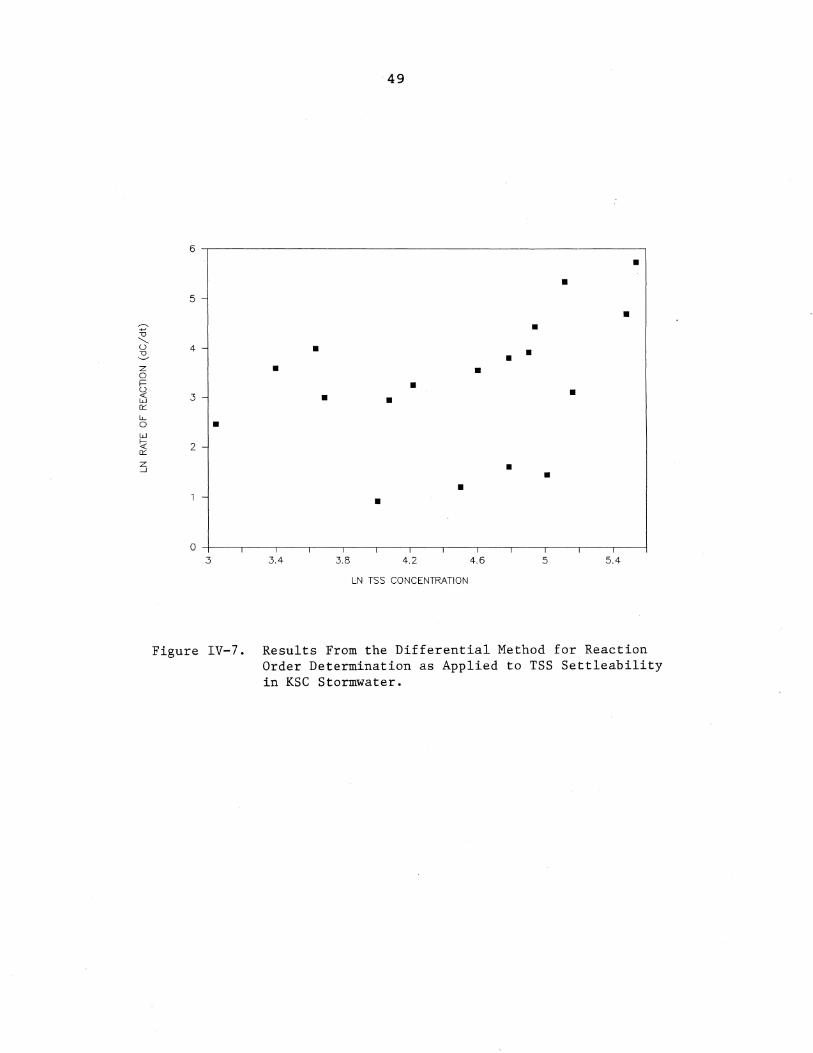
The reaction order is found by plotting reaction rate,
dC/dt, versus concentration, C, where the slope of the best
fitting line represents the reaction order. As Figure IV-7
illustrates, no best fit line could reasonably be applied.
Therefore after consulting work by Nix (1982) who noted
that TSS settleability is fairly represented by first-order
kinetics, it was decided to use the simple first-order
removal equation:
,-.. +' U
'--u .::., z 0 f= u L5 0:::
LL 0 w I;:( 0:::
Z ....J
49
6
• •
5 -
• •
4 • • • • • •
3 • • • •
2 -
• • •
1 - •
0 3 3.4 3.8 4.2 4.6 5 5.4
LN TSS CONCENTRATION
Figure IV-7. Results From the Differential Method for Reaction Order Determination as Applied to TSS Settleability in KSC Stormwater.

50
C/Co = 1 - (Rmax * (1 - EXPA(-kt»)
where Co = initial concentration (mg/L)
Rmax = maximum removal fraction
k = rate constant (l/hr.)
t = detention time (hrs.)
Rmax and k were adjusted by trial and error until a
reasonable fit of the scatter plot was obtained. A
"reasonable fit" was based on experience and visual
inspection. The selected coefficients are:
Rmax = 0.85 (Nix (1982) ; Whipple and Hunter (1981) suggested 0.75 for TSS).
k = 0.43 (Nix (1982) suggested that 0.108 was reasonable for stormwater effluent).
(5)
The results of this trial and error fit to the raw data are
shown in Figure IV-8. The raw settleability data are shown
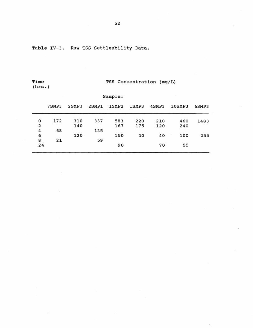
in Table IV-3.
Rating Curve for TSS Load
Because of the difficulty in predicting TSS loads based
on the physics of buildup-washoff processes, loads are
commonly predicted using empirical equations such as rating
curves. Field measurements on stream and channels often
warrant application of a simple empirical relationship
between suspended load and discharge, of the form:

0.9
0.8
0.7
0.6 ff) ff) f-
a 0.5 u "- • u
0.4 • 0.3 • 0.2
• 0.1
0 0 4
•
•
•
• • • 8
MEASURED
51
clco = 1-(O.85*(1-@exp(-0.43*t))) Settling Depth = 1.2 Feet
12 16 20
TIME (HOURS) PREDICTED
24
Figure IV-S. Results of Settleability Tests for Total Suspended Solids Load in KSC Stormwater Effluent.
52
Table IV-3. Raw TSS Settleability Data.
Time TSS Concentration (mgjL) (hrs. )
Sample:
7SMP3 2SMP3 2SMP1 lSMP2 lSMP3 4SMP3 10SMP3 6SMP3
0 172 310 337 583 220 210 460 1483 2 140 167 175 120 240 4 68 135 6 120 150 30 40 100 255 8 21 59 24 90 70 55

53
where M = total load (mass)
V = runoff volume, and
a,b = regression coefficients.
(6)
The results of the simple regression analysis on the
transformed data are presented in Figure IV-9. The
prediction of the rating model versus actual measured data
is shown in Figure IV-10. Note the general increase for
.these two locations in the variance of loads as runoff
volume increases. A number of field studies have shown
loading data as scattered as these (Diniz and Espey, 1979;
Smolenyak, 1979). For example, after using a log-log
transformation of TSS data for 260 events, Smolenyak (1979)
reported a coefficient of determination of 0.56 from
regression analysis.
Channel characteristics at KSC undergo continual
evolution (e.g. from scraping to various densities and
heights of vegetation) over the year. It is hypothesized
that this accounts for much of the variability. More data
over a number of channel cleaning and revegetation cycles
would likely produce a better rating curve. However for
analysis, this relationship provides general runoff loading
characteristics as long as its uncertainty is considered in
the study conclusions and recommendations.

o g [f) [f) I--I-Z w GJ Z ...J
54
9 ,------------------------------------------------------------,
• N = 8
• • •
7
• 6 •
5
4
• 3 4------,-----,,-----,-----,------,------r-----,------r----~
8 9 10 11 12
LN EVENT RUNOFF VOLUME (FT ~3)
Figure IV-9. Simple Regression of Transformed Event Runoff Volume and Event Total Suspended Solids Load Data.

55
7
6 •
5 Load Mass = 0.00415W~ 1.15 I/) III
2.~ OCll 4 <{"O OC -,0
CIl (/):::J (/)0 f--'c 3 f-f-'-' Z w GJ •
2 • •
• • o 40 80 120 160 200 240
(Thousands) EVENT RUNOFF VOLUME (FT ~3)
Figure IV-lO. Relationship Between Event Runoff Volume and Event Total Suspended Solids Load.

CHAPTER V
HYDROLOGIC SIMULATION OF THE STUDY AREA
Introduction
Changes in land use in a watershed can significantly
alter its natural hydrologic response. A quantified
prediction of the change in hydrologic response for a
specified change in land use is fundamental to engineering
design and the assessment of environmental impact.
Relatively simple estimates of runoff as a function of
land use are commonly performed for certain specified areas
within the Indian River Lagoon catchment. Typically, these
computations are performed for engineering design and are
based on synthetic design storm events. Only two documented
attempts at modeling large SUb-catchments within the Indian
River Lagoon basin were located. A preliminary assessment
study of the 13 square mile Turkey Creek sub-catchment
(Suphunvorranop and Clapp, 1984) used the STORM model (U.S.
Army Corps of Engineers, 1977) to simulate total runoff
hydrographs and pollutant concentrations. This model was
selected because it was readily available and required less
56

57
input data than other water quality models. Unfortunately
because of a lack of continuous streamflow records and
backwater effect from the lagoon, no calibrations were
performed. In addition, the STORM model is limited in
coastal areas of Florida as it does not include groundwater
contributions to runoff. Da Costa and Glatzel (1987)
conducted a simulation of "30 year monthly normal
conditions" of runoff to the entire Indian River Lagoon
using basic water budget methods outlined in Dunne and
Leopold (1978). The major weakness of this approach is it
lacks an accounting of groundwater discharge to the dense
network of drainage canals, and such large time steps may be
inadequate for receiving water analysis. Nevertheless, for
Crane Creek, a small stream, they state that the agreement
between field observations and simUlation was within 10%;
however, no data were presented.
Goodness of Fit criteria
Deterministic hydrologic model accuracy is largely
determined by (1) available input, (2) monitoring data on
system response to varying inputs, and (3) the degree of
model calibration and verification to mUlti-events over
time. After considering problems associated with generating
synthetic streamflow from models, Stedinger and Taylor
(1982) concluded that the impact of parameter uncertainty is
much greater than that of the selection between a simple and

58
a relatively complicated model. They went on to recommend
that given what is actually known about a basin's hydrology,
model parameter uncertainty should be incorporated into
simulation studies to obtain realistic and honest estimates
of watershed response. However for many applications, it is
highly impractical to obtain precise uncertainty information
on what may be hundreds of parameters required to describe
watershed response. Current practice assumes that the
simplest model that will describe the system for the given
input data should be used (Bedient and Huber,~1988). These
are typically lumped parameter models that are calibrated to
actual performance data.
Calibration involves minimization of deviations between
measured field conditions and model output by adjusting
parameters within the model. Verification is the process of
checking the model calibration using an independent set of
data.
Depending on the objectives, simulation of stormwater
discharge, baseflow, and hydrologic/hydraulic control in a
coastal drainage canal could require emphasis on the close
prediction of total annual flow, average monthly flow
volumes, peak flows, low flows, or specified events.
However, Heaney et ale (1986) noted that equally successful
prediction of each of these flow statistics using the same
set of parameters is highly improbable. Sensitivity analysis
for a lumped parameter model often shows a change in one
parameter may improve one aspect of the calibration though

59
reducing the "goodness of fit" of another aspect. Jewell et
ale (1978) even found that different storm events resulted
in different calibrations and different predictions.
Therefore, to make decisions on changing parameter values
during the calibration of the model, goodness of fit
criteria need to be established based on the objectives of
the study. The objectives for this simulation experiment
were the minimization of the average differences between
measured and predicted total event runoff volume, peak flows
for specified events, and total event pollutant load.
This discussion has highlighted some of the limitations
of watershed scale hydrologic simulation. Despite this,
models still provide the most logical and scientifically
advanced approach to understanding the hydrologic behavior
of complex watershed and water resources systems (Bedient
and Huber, 1988).
Runoff Block
The storm Water Management Model (SWMM) simulates real
storm events on the basis of rainfall and other
meteorological inputs and system (catchment, conveyance,
storage/treatment) characterization to predict outcomes in
the form of quantity and quality values (Huber and
Dickinson, 1988). The model consists of four main
computational blocks (RUNOFF, TRANSPORT, Storage/Treatment,
and EXTRAN) and six service blocks. The TRANSPORT,
60
storage/Treatment, and EXTRAN blocks may all use input and
provide output to any block, including themselves.
The Runoff Block (RUNOFF) has been developed to simulate
both quantity and quality runoff phenomena of a drainage
basin and the routing of flows and contaminants to major
conduits. Used in either the single event or continuous
mode, the program takes a step-by-step accounting of
rainfall, infiltration losses to pervious areas, surface
detention, overland flow, soil moisture, evaporation,
groundwater discharge to drainage canals, gutter flow, and
the constituents washed into inlets, leading to the
calculation of a number of inlet hydrographs and
pollutographs (Huber and Dickinson, 1988). Sub-catchments 4
and 5 in the study area (see Figure IV-I, p. 34) were
monitored, RUNOFF was calibrated and verified to these data
and then applied to the remainder of the study area using
Geographical Information System (GIS) data and other
discretized data. These two sub-catchments are
representative of developed areas of the study area. RUNOFF
is most sensitive to parameters that describe the degree of
development (e.g. impervious area, drainage channel
geometry) .
Runoff Quantity Data Input
Runoff Block parameters for sUb-catchments 4 and 5 are
listed in Table V-I. The average slope was found by

61
Table V-1. Runoff Block Parameters for Sub-Catchments 4 and 5.
PARAMETER
Area
Characteristic width
Percent hydraulically connected imperviousness
Slope
Manning's roughness Impervious Pervious Channel
Horton parameters Hydraulic conductivity Initial infiltration rate Decay rate of infiltration
Conduit parameters Length width Invert ope Side slope Full depth Weir height
Groundwater parameters Porosity wilting point Field capacity Hca pca Fraction of max. ET rate in upper zone
Deep recharge Maximum depth ET
UNITS
ac.
ft.
in./hr. in./hr. l/sec.
ft. ft.
ft. ft.
CATCHMENT
4
167
4000
18
0.00012
0.013 0.25 0.044
5.0 10.0 0.00115
4000 15 0.00035 1/2 4.0 0.04
0.3 0.03 0.05 10 15 0.001
5
133
3000
15
0.00012
0.013 0.25 0.044
5.0 10.0 0.00115
4000 15 0.00035 1/2 4.0 0.04
0.3 0.03 0.05 10 15 0.001
in./hr. 0.00003 0.00003 ft. 4.5 4.5
Note: Hca = Calibration parameter, estimates change in unsaturated hydraulic conductivity with change in soil moisture.
pca = Change in soil tension/change in soil moisture.

62
calculating the path length between a point on the edge of
the catchment to the catchment outlet, and dividing the path
length by the change in elevation. The catchments
essentially have a uniform, flat slope. Percent of
hydraulically connected impervious area was based on a
calibrated fraction of the total impervious area as
determined by the updated Industrial Area GIS land use
files. After calibration, the fraction was found to range
from 0.33 to 0.38. For unca.1ibrated sub-catchments, 35% of
the impervious area was assumed to be hydraulically
connected.
Soils in the study area are primarily of the Spodosol
Order with much of them having been classified as Urban type
(Huckle et al. 1974) which originated mainly from Immokalee
soils. Lesser areas of Felda, Basinger, Anclote, and Myakka
soils are also found. Soil types and parameters were lumped
and assumed to be represented by Immokalee soils. The
Horton infiltration equation option was used. Maximum
initial infiltration and the decay rate of infiltration
were assumed to be represented by published data summarized
in the SWMM manual (Huber and Dickinson, 1988) for dry sandy
soils. The asymptotic infiltration rate is essentially
equal to saturated hydraulic conductivity. For Immokalee
soils, Carlisle et al. (1985) report a value of 4 in/hr. for
saturated hydraulic conductivity. Using in-situ slug test
procedures in the study area, Clark Engineers-Scientists,

63
Inc. (1987) reported hydraulic conductivity ranging from 4
to 7.5 in/hr. A value of 5.0 in/hr. was selected for use in
RUNOFF.
Manning's n values were selected from tables based on
average type ground cover and from the rating curve
development. Average monthly pan evaporation data were from
National Weather Service values for Vero Beach,Florida
published by Heaney et al. (1984). The catchment width
parameter in RUNOFF represents the physical width of
overland flow for the catchment; however, in lumped
catchments it is used as a primary calibration factor.
After calibration, a rule of thumb used to determine
characteristic width for uncalibrated sub-catchments was to
calculate it from catchment area with a catchment length of
1800 feet, assuming a rectangular catchment. Catchment
length physically represents the distance overland flow must
travel to reach a conduit (channel flow). A single conduit
with a "dummy" mini-rectangular weir outfall was used for
each sub-catchment to provide routing delay and account for
in channel dead storage (due to depressions in the channel
and culvert invert elevations being above channel invert
elevations). The conduit length was used as a fine tuning
calibration parameter; however, it was based on the length
of the trunk or main drainage channel of the catchment.
In Florida, where land slopes are flat and water tables
are high, the primary drainage pathway is often through the

64
surficial aquifer and the unsaturated zone above it. Capece
et ale (1984) reported that in Florida Flatwood areas a
storm will cause a rise in the water table which results in
a natural detention release to the drainage canals. A
simple estimate by Clark Engineers-Scientists, Inc. (1987)
indicated that groundwater discharge to drainage canals
accounted for 11% of the water budget for KSC while direct
runoff accounted for less than 2%. This process was also
observed during the data collection phase of this project
and later hydrologic simulation experiments suggested that
this phenomenon was responsible for a large percentage of
the runoff from the study area (see simulation results
section).
RUNOFF, in the latest version of SWMM (Version 4),
contains a subroutine to account for subsurface flow routing
(groundwater seepage to canals). The groundwater subroutine
simulates two zones, an upper unsaturated zone and a lower
saturated zone. Inflow into the groundwater subroutine is
calculated in the infiltration subroutine. The flow from
the unsaturated to the saturated zone is controlled by a
percolation equation. Losses and outflow from the lower
zone can be via deep groundwater recharge, saturated zone
evapotranspiration, and groundwater flow. Groundwater flow
is a user-defined power function of water table stage and,
if chosen, depth of water in the discharge channel (Huber
and Dickinson, 1988).

65
The general groundwater discharge equation provided by
the model is as follows:
GWFLW = A1 * (01-BC)AB1 - TWFLW + A3 * 01 * TW (7)
and
TWFLW = A2 * (TW-BC)AB2 (8)
where
GWFLW = beginning of time step groundwater flow rate (per area),
TWFLW = channel water influence flow rate (per area),
A1,A2 = groundwater and channel water influence coefficients,
A3 = coefficient for cross-product,
B1,B2 = groundwater and tailwater influence exponents,
BC = elevation of bottom of channel,
TW = elevation of water in channel, and
01 = average water table head.
This general equation was given the functional form of the
oupuit-Forcheimer approximation (Bouwer, 1978) for drainage
to an adjacent channel by setting flow coefficients and flow
exponents as follows:
(9)
and
A2 = 0, B1 = 2
where K = hydraulic conductivity = 10 ft./day (5in./hr.)
L = length of flow for groundwater influenced by
channel.

66
Based on observations at KSC reported by Clark Engineers
Scientists, Inc. (1985), L ranges from 300 to 500 feet.
Therefore, the reasonable range for A1 and A3 is from 2.22E-
4 to 8.0E-5 (in./hr.-ft. A 2). During the calibration
process, a value of 1.2E-4 (in./hr.-ft. A 2) was found to
provide acceptable results.
Initial upper zone moisture content and water table
elevation for calibration events were estimated using
continuous simulation prior to the event~ Initial estimates
of porosity, field capacity, and wilting point 0.46,
0.13,and 0.038, respectively) were made from published data
(Carlisle et al., 1985) for Immokalee soils. However, such
data produced poor matches of channel baseflow, the observed
hydro graph characteristics indicative of groundwater flow
(slow prolonged discharge at the tail of the stormwater
runoff hydrograph), and groundwater table fluctuations.
Therefore these parameters in effect also became calibration
parameters. As a guide in estimation, Bennett's (1988)
lumped parameter estimates were used. Using a calibrated,
lumped parameter spreadsheet simulator to predict water
table behavior in Merritt Island, Florida, Bennett (1988)
found values for porosity and field capacity of 0.2 and
0.0275, respectively, to provided good matches between
observed and simulated groundwater table fluctuations.
Percolation calibration parameters used in the SWMM manual
for an example for the Cypress Creek, Florida watershed were
also used for this study area. The KSC Groundwater Survey

67
(Clark Engineers-Scientists, Inc., 1987) provided data on
(1) the rate of evapotranspiration (ET) from the water
table, (2) the depth limit of ET from the soil, and (3) the
rate of "effective" surficial aquifer recharge.
Calibration and Verification.
A randomly selected mix of event periods, generally
distributed over the 1988 year, was used for calibration and
verification. Calibration was done for average conditions
across several storms by maintaining the same parameter
values for each until predictive error was a minimum for all
events. From sensitivity analyses, it was deduced that
percentage impervious area, and groundwater parameters would
be the primary volume calibration factors.
Characteristic width and routing conduit parameters
change the shapes of the hydrographs and improve and
predicted peak flows. The agreement between measured and
predicted volumes and peak flows for Catchment 4 are shown
in Figures V-1 and V-2. The agreement for Catchment 5 are
shown in Figures V-3 and V-4. Some Catchment 4 multi-event
hydrographs of measured and predicted flows from the
calibration and verification runs are shown in Figures V-5
and V-6; similar hydrographs for Catchment 5 are shown in
Figures V-7 and V-8. Comparisons of measured and predicted
groundwater hydrographs for Catchments 4 and 24 are shown in
Figures V-9 and V-10, respectively.

16
15
14
13
12 (j)
11 u.. S "0
10
-1l 9 '0 i!: 8 "-w 7 c.:>
"" « 6 I 0 (f)
is 5
4
3
2
0 0 2
• +
•
68
4
+
6
DISCHARGE measured (CFS) • CALIBRATION + VERIFICATION
•
8
Figure V-i. Peak Flow Results from the Calibration and Verification Runs--Catchment 4.
10
5 ,-------------------------------------------------------,
-;;, W I o Z .;::.
3 •
2
+
+.
o ~--+~------._----------._--------_.----------~----------~ o 2 4
VOLUME measured (INCHES/167 ACRES) • CALIBRATION + VERIFICATION
Figure V-2. Total Flow Results From the Calibration and Verification Runs--Catchment 4.

69
15
14
13
12
1f 11
~ 10
-0 9 2 + 0 'U 8 Q)
a. 7 w '-' Cl:: 6 <{ I U 5 If) • is
4 + • 3
2
• • 0
0 2 4 6 8 10 12 14
DISCHARGE actual (CFS) • CALIBRATION + VERIFICATION
Figure V-3. Peak Flow Results from the Calibration and Verification Runs--Catchment 5.
0.9
0.8
'iiJ w 0.7 Cl:: u <{ ...,
0.6 ..., "-If) • W I u 0.5 z .;::,
-0 0.4 2 0 'U • + Q) a. 0.3
w ::E => 0.2 ...J
+ 0 >
+ 0.1 • +
0 0 0.2 0.4 0.6 0.8
VOLUME actual (INCHES/133 ACRES) • CALIBRATION + VERIFICATION
Figure v-4. Total Flow Results from the Calibration and and Verification Runs--Catchment 5.
70
11
10 -
9 -
8 -
8 7 -"--S
6 w (!> D::: « 5 I U (f)
is 4
3
2
2.6 2.8 3 3.2 3.4 3.6 3.8 4 (Thousands)
TIME (HOURS SINCE 1 JAN 88) ----- MEASURED -- PREDICTED
Figure V-5. Measured and Predicted Hydrographs from a Calibration Run on Catchment 4. April 12, 1988 through June 15, 1988.
3.5
3
2.5
E S 2 w Cl D:::
~ 1.5 u (f)
6
6.7 6.9 7.1 7.3 (Thousands)
TIME (HOURS SINCE 1 JAN 88, OOOOHRS) MEASURED -- PREDICTED
Figure V-6. Measured and Predicted Hydrographs from a Verification Run on Catchment 4. October 10, 1988 through November 2, 1988.

f S w (!) 0:: « I C,) (/)
0
3.5
3
2.5
2
1.5
0.5
71
, , .... - -\_1 , , , , , , , , , ,
I
"'--- ..... ,'-
o 1-------,-------,-------~-,~'------,_------r_------r_------r_----~ 1.52 1.54 1.56 1.58 1.6
(Thousands) TIME (HOURS SINCE 1 JAN 88, OOOOHRS) measured -- predicted
Figure V-7. Measured and Predicted Hydrographs from a Calibration Run on Catchment 5. March 4, 1988 through March 7, 1988.
,-,
~ S w (!) 0:: « I C,) (/)
0
1.4 ,---------------------------------------------------,----------,
1.3
1.2
1.1
0.9
0.8
0.7
0.6
0.5
0.4
0.3
0.2
0.1 -
0 6.7
! I,
"\ " " "
6.9 7.1 (Thousands)
TIME (HOUR SINCE 1 JAN 88, OOOOHRS) measured -- predicted
, , , , " ." " " "' 1111
:lj'~' 1111 1111 I \!t..
7.3
Figure V-8. Measured and Predicted Hydrographs from a Verification Run on Catchment 5. October 10, 1988 through November 2, 1988.

-::? (/)
::1'
~ z 0 i= ::; w ...J W
W ...J (l)
,::: '" W f-« 3<
-::? (/)
::1' --z 0 i= ::; w ...J W
W ...J (l)
,:::
'" w ~ 3<
7
6
5
4
3
2
o
72
2 4 6 (Thousands)
TIME (HOURS SINCE 1 JAN 88, 0000 HRS.) -- PREDICTED <> MEASURED
8
Figure V-9. Predicted and Measured Groundwater Table Elevation for Observation Well BAS18 Located in Catchment 4.
7
6
5
4 +
3
2
o 246 (Thousands)
TIME (HOURS SINCE 1 JAN 88, 0000 HRS.) -- PREDICTED + MEASURED
8
Figure V-10. Predicted and Measured Groundwater Table Elevation for Observation Well BAS20 Located in Catchment 24.

73
It is hypothesized that a major portion of the error is
accountable by variable rain distribution over the
catchment, error in using rain data 1.1 miles from the study
area, and exfiltration of runoff from channels during the
dry season. Other error may be introduced by the model's
simplistic representation of groundwater discharge to the
channels. Noted limitations are the lack of accounting of
exfiltration from the channels.
Runoff Quality
Available deterministic models usually compute
stormwater quality via a series of steps. First
accumulation of pollutants during dry weather buildup is
estimated. Then estimates of the accumulated pollutants
that are washed off (washoff) is made. Since the processes
of accumulation, redistribution, washoff, transport, and
dispersal are complex in nature, a general model for the
complete process suitable for application to all catchments
has yet to be developed (James and Boregowda, 1985).
However, with sufficient site-specific calibration data,
reasonable predictions can be made using empirical
relationships (e.g. rating curves) or simple, physically
based functions found in most general water quality models
(Huber, 1985).

74
Data Input
Water quality parameters used in RUNOFF are listed in
Table V-2. Three buildup equation forms are available in
RUNOFF, power-linear, exponential, and Michaelis-Menton. A
linear, no upper limit buildup formulation for particulate
was selected as a starting point for pollutant buildup
calibration for this study. Because development in the
study area is relatively mature and observation suggested
that channel scour was the principal contributor of
suspended solids, the functional dependence of the buildup
parameters was based on channel length rather than catchment
area. For pollutants other than particulates, this approach
would not be appropriate (e.g. nutrients, metal, and
hydrocarbons are better related as a function of catchment
area). Channel length for pollutant buildup was based on
total channel length rather than main channel length. To
account for ambient concentrations of TSS, it was assumed
that groundwater flow contributed 1 mg/L of TSS. The number
of dry days before a rain event was estimated to be 4.0
days; this corresponds to the mean interevent rain period
for Melbourne, Florida (Heaney et ale 1984). The buildup
parameters were used for calibration of RUNOFF water quality
predictions. Washoff estimates of suspended solids were
based on the rating curve developed from study area data
(see Chapter IV).

75
Table V-2. Runoff Block Water Quality Parameters.
PARAMETER VALUE
Buildup No. of dry days before
the start of storm Type of buildup calculation (KCALC) Functional dependence of buildup
parameters (KACGUT) Buildup limit
Buildup exponent Buildup coefficient
Washoff Type of washoff calculation (KWASH) Exponent for washoff rate (WASHPO) Washoff rate coefficient (RCOEF)
4 Power-linear (1)
Gutter length (0) 1.0E+6 lbs/100 ft.
1.0 5.0
Power (0) 1.15 40
Note: Parentheses indicate SWMM input variable nomenclature.

76
Calibration
For water quality predictions, calibration of RUNOFF
centered around a trial-and-error procedure to determine the
ideal combination of buildup rate coefficients that result
in a satisfactory match of the measured and predicted event
suspended solids loads. RUNOFF was calibrated for average
conditions across several storms to reduce predictive error
and increase confidence. The agreement between measured and
predicted event loads of suspended solids is shown in Figure
V-II. The loading predictions look reasonable with the
exception of event TSS5-4 which appears to be an outlier.
Channel scraping (cleaning) during the week of this event
explains the extraordinarily high loading measured. The
presence of outliers in a data set creates analysis
problems. They distort statistical measures and, in this
case, the outliers are generally neither periodic, nor
predictable. Fortunately, this outlier is explainable and,
therefore excluded from the calibration analysis as it is
unrepresentative of "average conditions".
variations in the runoff quantity predictions contribute
to error in the predicted loads. For example, a slight
difference between observed and predicted runoff discharge
concurrent with a high rate of mass transport, contributes
further to the error in estimating pollutant loads.
Because the goal of this project was to estimate the
loadings to the estuary and to examine relative

77
2.6
2.4
2.2
• U1 2 0}
.::::::. 1.8 0 <{ 0 1.6 • ---'~ I/)ffl 1/)-0
1.4 I- c • 0 <> I-ffl z:>
1.2 W o 2Jt 0 w I-u 0.8 is w Q::
0.6 0...
0.4
0.2
0 0 2 4 6
(Thousands) MEASURED TSS EVENT LOAD (LBS)
• CALIBRATION -- IDEAL <> OUTLIER
Figure V-ll. Goodness of Fit of Event Total Suspended Solids Load.

78
effectiveness of multi-objective surface water management
strategies, the model results were deemed acceptable.
Estimates of Loadings from the Industrial Area Catchment
An objective of this study was to estimate typical
annual freshwater discharge (from both overland runoff and
groundwater seepage to channels) and pollutant loadings
(represented by TSS) under existing land-use conditions and
future development for the study area. Future research
plans include incorporating such estimates in a receiving
water response analysis.
From the environmental management perspective, receiving
water may respond slowly to input (particularly estuaries
where the response time has been estimated at days to weeks
(Driscoll, 1979». It is seldom necessary to consider more
than the total pollutant load from a storm for receiving
water analysis. Detailed pollutographs are usually not
required since short time-step variations are strongly
dampened by the receiving water response (Huber, 1985). For
example, Bartleson (1988) suggests that high concentrations
of dissolved nutrients can increase epiphytic algae coverage
and reduce light, thus decreasing seagrass growth. However,
short term pulses of nutrients or turbidity may have little
effect on the seagrass biomass. stresses applied relatively
evenly over large estuarine areas will be the most difficult
for seagrass to tolerate (Florida Department of
Environmental Regulation, 1987).

79
Data Input
Calibrated input files for sub-catchments 4 and 5 were
extrapolated to represent the entire study area using rules
developed during calibration. A schematic diagram catchment
and associated channel numbers as represented in the model
of the study area is shown in Figure V-12. Parameters
varying between catchments under existing conditions are
summarized in Table V-3. Since "typical" loadings to the
receiving water are sought, a continuous simulation of
existing development was driven by the hourly precipitation
record for 1951 at the Melbourne station. As noted in
Chapter IV, 1951 was a "typical" rainfall record year. Sub
catchments 3 and 24 were simulated as "shoreline" catchments
where the average surface elevation is approximated at 5.0
ft MSL and the initial water table elevation is 3.7 ft.
MSL. The channel for sub-catchment 1 is heavily vegetated
(not maintained) and is assumed to produce little TSS
loading due to scour. Therefore, channel 111 for sub
catchment 1 is assumed to have only 100 feet of its 6200
feet available for "pollutant buildup".
The timing of discharges to the receiving water is
controlled by the backwater conditions of the lagoon.
Because of a lack of long-term lagoon elevation data,
"typical" lagoon water level elevation (backwater elevation)
as a function of time could not be generated. Therefore
continuous hydraulic routing of runoff to the lagoon was not

Catchment 444 4
N Catchment
24
INLET
txtx ~
Banana River
ca~h~ent Catc;ment I ca:~entl ~
IS 111/~ Catchment I ~ / ~ ~
555 5
~
INLET
Figure V-12. Schematic of the RUNOFF Simulation for the Entire Study Area.

81
Table V-3. Runoff Block Parameters for the study Area.
Hydraulically Initial Avq. sub- Characteristic Connected Channel water Table Grade Catchment Area width Imperviousness Length Elev. Elev.
(ac. ) (ft. ) (%) (ft. ) (ft. MSL) (ft. MSL)
1 577.2 13,970 0.0 6,200 4.5 8.0
3 489.3 11,841 4.5 4,000 3.7 5.0
4 167.0 4,000 18.0 4,000 4.5 8.0
5 133.0 3,000 15.0 4,000 4.5 8.0
15 218.5 5,290 15.0 3,600 4.5 8.0
24 315.6 7,640 5.0 6,000 3.7 5.0

82
attempted. Residence time in the trunk channels is
estimated at less than 2 hours under the existing
configuration. However, no adjustment factor was applied
to account for deposition in the trunk channel areas
influenced by backwater. Although a relatively crude
technique, it represents the best available procedure to
roughly estimate solids loadings to the estuary until long
term data sets on lagoon water levels are generated.
Detailed hydraulic analysis of TSS transport through the
channels is futile until backwater conditions become
predictable.
The processes involved in the transport of suspended
solids at channel mouths to the lagoon are complex.
Transport is influenced by such factors as the riverine-like
discharges from the channels, quasi-periodic aeolian tides,
and saline water enhanced coagulation of hydrophobic
colloids (and sedimentation) in the sediment laden
freshwater flows into the estuary (the double-layer
compression aggregation mechanism (Manahan, 1984». Exports
will change as the hydrology is switched from a stream
dominated system during wet-weather to an aeolian tide
dominated system. However, after reviewing the Ryan and
Goetzfried (1988) dry-weather data at the mouth of Buck
Creek, suspended solids transport is dominated by wet
weather events. Unfortunately, this area of the drainage
network can only be addressed qualitatively in this study
until additional data are generated.

83
Future land use change in the study area and the time
frame for any change are highly unpredictable. Therefore
for these simulation experiments, the concept of maximum
buildout is presented. The definition of maximum buildout
is somewhat subjective and will likely vary between agencies
and engineering/planning offices. For the purposes of this
research, maximum buildout is based on the existing
development in sub-catchments 4 and 5. It is assumed that
these catchments are fully developed. Calibration of the
model suggests that 18% of a "fully developed" catchment
will be hydraulically connected impervious area. The
construction of additional drainage channels was estimated
based on existing facilities layouts. The projection of
buildup channel length was based on the drainage channel
density in sub-catchments 4, 5, and 15. Details of this
projection are found in Table V-4. A summary of existing
and "maximum buildout" conditions in the study area is shown
in Table V-5. The actual RUNOFF input files used are found
in Appendix B.
Groundwater discharge to the drainage network can be
expected to increase with increased development (maximum
buildout). However in RUNOFF, groundwater discharge is
calculated as a function of catchment area. This approach
does not represent the length of the actual seepage face.
Therefore the increase in seepage face length expected with
increased development was not physically represented. Any
difference in the predicted groundwater discharge between

84
Table V-4. Calculations of Channel Buildup Length for Water Quality simulation in RUNOFF.
Assumptions:
Catchments 4, 5, and 15 represent typical buildout density and drainage channel density.
Catchment
----------Catchment 4
Catchment 5
Catchment 15
Area (ac. ) -----
167
133
218.5
Existing Buildup Channel Length
(ft. )
13,800
8,700
16,200
Mean Drainage Density =
Drainage Density (ft./acre)
82.6
65.4
74.1
74
Therefore, the formula for determining maximum buildout
buildup channel length is as follows:
«Catchment Area) - Unbuildable Catchment Area) * 74 ft./acre
Unbuildable Catchment Area = Wetlands and Surface Water.
Maximum Buildout Buildup Channel
Catchment Unbuildable Area Buildable Area Length (ac. ) (ac. ) (ft. )
--------- --------- --------- ---------
1 10 567 41,958
3 120 369 27,306
4 0 167 13,800
5 0 133 8,700
15 0 218.5 16,200
24 30.5 285 21,090
85
Table V-5. Development Scenarios for the Industrial Area.
PARAMETER
SUB-CATCHMENT 1: Area Percent hydraulically
connected imperviousness Channel length Buildup channel length
SUB-CATCHMENT 3: Area Percent hydraulically
connected imperviousness Channel length Buildup channel length
SUB-CATCHMENT 4: Area Percent hydraulically
connected imperviousness Channel length Buildup channel length
SUB-CATCHMENT 5: Area Percent hydraulically
connected imperviousness Channel length Buildup channel length
SUB-CATCHMENT 15: Area Percent hydraulically
connected imperviousness Channel length Buildup channel length
SUB-CATCHMENT 24: Area Percent hydraulically
connected imperviousness Channel length Buildup channel length
EXISTING MAXIMUM BUILDOUT
577.2 ac.
0.0 6200 ft. 100 ft.
489.3 ac.
4.5 4000 ft. 6600 ft.
167 ac.
18 4000 ft. 13,800 ft.
133 ac.
15 4000 ft. 8700 ft.
218.5 ac.
15 5600 ft. 10,200 ft.
315.6 ac.
5 6000 ft. 4000 ft.
577.2 ac.
18 9000 ft. 42,958 ft.
489.3 ac.
18 5000 ft. 27,300 ft.
167 ac.
18 4000 ft. 13,800 ft.
133 ac.
18 4000 ft. 8700 ft.
218.5 ac.
18 5600 ft. 10,200 ft.
315.6 ac.
18 7640 ft. 21,000 ft.

86
existing and maximum buildout conditions has no physical
meaning. In hindsight, groundwater discharge can be
calculated as a function of channel length rather than
catchment area by incorporating seepage face length in the
discharge coefficients in the model's general groundwater
discharge equation. This coefficient development is shown
in Appendix C.
Results
The predicted annual water budget for the study area
drainage network under existing land use conditions is shown
in Figure V-13. Groundwater inflow accounts for 87% of the
annual discharge from the study area. However, its
contribution varies both within the catchment and within the
storm event. For example, Figures V-14 and V-15 show
groundwater discharge in upland and lowland subcatchments.
During wet-weather, groundwater discharge is reduced if not
discontinued. Combined discharge from the study area for a
typical year is shown in Figure V-16. A comparison of
predicte~ annual loads for existing land use and maximum
buildout is shown in Table V-6 and by month in Figures V-17
and V-18. The model estimates that if development of the
study area were to occur to its maximum potential, the
annual discharge of freshwater would increase by 18% and the
annual TSS load would increase by 290%.

87
*************** ••• ***** •• *****.************* ••
* CONTINUITY CHECK FOR CHANNEL/PIPES * .******************** ••• ******** •• ******** ••••
INITIAL CHANNEL/PIPE STORAGE •.•••••••••••••• FINAL CHANNEL/PIPE STORAGE •..••••••••••••••• SURFACE RUNOFF FROM WATERSHEDS •.•••.••••••.• GROUNDWATER SUBSURFACE INFLOW •••.••••••••••• EVAPORATION LOSS FROM CHANNELS ••.•.••••••••• CHANNEL/P I PEn NLET OUTFLOW ••••••.••••••••••• INITIAL STORAGE + INFLOW •••.•.•••••••••••••• FINAL STORAGE + OUTFLOW ••••••••••.•••••••••• *********** •• ***** •• ************************
* FINAL STORAGE + OUTFLOW + EVAPORATION - * * WATERSHED RUNOFF - GROUNDWATER INFLOW - * * INITIAL CHANNEL/PIPE STORAGE * * * * FINAL STORAGE + OUTFLOW + EVAPORATION * ******************************** ••• *********
ERROR •.•••••••.•••••••••••.•.•••••..•.••••••
CUBIC FEET 2.900720E+05 7.393456E+04 1.544678E+07 9.651181E+07 2.246527E+06 1.107775E+08 1.122487E+08 1.130979E+08
INCHES OVER TOTAL BAS I N
0.042 o • 011 2.239
13.990 0.326
16.057 16.271 16.394
0.751 PERCENT
***************************************************
* CONTINUITY CHECK FOR SUBSURFACE WATER * ***************************************************
TOTAL INFILTRATION TOTAL UPPER ZONE ET TOTAL LOWER ZONE ET TOTAL GROUNOWATER FLOW TOTAL DEEP PERCOLATION INITIAL SUBSURFACE STORAGE FINAL SUBSURFACE STORAGE UPPER ZONE ET OVER PERVIOUS AREA LOWER ZONE ET OVER PERVIOUS AREA
*************** •• ************************.
* INFILTRATION + INITIAL STORAGE - FINAL * * STORAGE - UPPER AND LOWER ZONE ET -* GROUNDWATER FLOW - DEEP PERCOLATION
* *
* -------------------------------------- * * INFILTRATION + INITIAL STORAGE * **************** •• ************************
ERROR ••••..••••••••••.••••.••••••••••.•••
INCHES OVER CUBIC FEET SUBSURFACE
BASI N
2.876568E+08 41. 697 4.080912E+05 0.059 2.030482E+08 29.432 9.651181E+07 13.990 1.146781 E+06 0.166 1.117154E+08 16. 193 1.149681E+08 16.665 4.080912E+05 0.063 2.030482E+08 31.426
-4.184 PERCENT
Figure V-13. Predicted Annual Water Budget for the Study Area Under Existing Land Use Conditions.

88
1.CXXl 1---------1---------1-------- -1------ ---1--- ------1-- ---- --- I -- ------ - I --- ----- -1------- --\-- __ -- ___ I I
I
0.00:1 -
I
0.600 -
..
..
..
.. ... ... - .. ***** .. ... - ..
FUll * *** '**
IN
CFS
.. .. .. ...
.. .... .. .. ....
.. _ .. .. ....
.. _ .. .. ..... ... .. ....... - ... .. - .. - .. .. ..
0.400 - -.... ... .. - .. .. - .. .. ***** .. ** * ..... **"* *** ** .. .. ** .. ** .. ..
.. ** ***** **** *** I" ... .. --- -1- - .. .. .. - .. - .. .. - - .. .. .. - ... .. ..-
0.200 .. .. .. .. .. .. .. .. .. ..
O.CXXl .. --------- I ---------1--------- I ---------1--------- I --------- I --------- I --------- I ---------1--------- I
0.0 1CXXl.0 200).0 3OXl.0 400J.0 SOOJ.O 6000.0 700).0 !lXXI.O c;ro).O 10CXXl.0
I.CCATICN Nl. 4 TilE IN IQ.RS
Figure V-14. Groundwater Discharge under Existing Land Use in One Upland Subcatchment for a "Typical" Year.

89
2.0CKl 1·····-·· ·1------. -'1" ---'---1'- --- ---'1----- ----1---------1· ----.. -'1-' ---... ·1'·· ······1····· .... 1 I
I
1.600 •
I 1.200 •
• *
FLCW
IN
CFS
..... "'- '" 1* * . -
** ** • * '" ** * * *** ** * * *.
0.8Xl * * ** *** * -* '" .. * * ** *** * •• ** . '" . * ** * * * * * * *** * ** ** • '" * *** * * * ** • * * * '" '" ** * * * *** * * * ****** * '" '" *** • * ** * * * * ****** * • • • * • ** * * * * ****** * "'''' • * * •• * * * * ****** * "' . '" • • .* * * * * ****** * "'. • • * ** * • * ** ****** • '" '" • *
0.400 * .* * * * ** ****** • "'* * * * ** * * • ** ****** • * • '" * * ** * * * ** ****** * * • * * * ** * * * ** ****** * ** * * * ** * * * ** ***** * * ** * * * * * • * * ** * *** * * * ** * • * * * • * * ** ***** • * ** '" * * ** * * * ** ***** * • ** * * * * * * * * ** * *** * • • ** *'" * ** * * * ** • ***. • • ** *'"
O.COl *- -----**- I ......... , ••••• " .... ----**,., •• ,""'*'* ... ***** ... -******1" ......... __ .... I ...... -'**- --1- .. -***-- ... 1 .... ---- .. "'''-1
0.0 10CKl.0 2000.0 3CXll.0 4(0).0 5000.0 6(0).0 7IXXl.0 8XlO.0 9CO).0 100CKl.0
LOCATICN NO. : 24 TIlE IN IU.RS Figure V-iS. Groundwater Discharge Under Existing Land Use in One
Lowland Subcatchment for a "Typical" Year.

90
SO.COl 1---------1---------1---------1---------1---------1---------1---------1---------1---------1--------_1 1
1
1
4O.COl -
1
3O.COl -
* * * * * * * * * * * * * * *
* * * * * * * *
* * * * *
RIJO'F * * * * * * * *
IN * * * * * * * *
CFS * * * * * * * * * * * *
2O.COl - * * * * * * * *
* * * * * * * * * * * • * * - -* * * * ** -* * * * ** **
* -* * * ** ** I * -* * * ** -1 * -* * * * * ** -
10.COl - * - * * * * ** ** * - * * * * ** * ** * - * * * * ** * ** * - ** * * * - ** ** * - ** * - * * *- -* - - * - ** ** * * **** * - * ** ** - - ** * -
1- - * -- ** -•••••••••••• - * - - * * -* - * - •••••• *111 •• 111 ••••• * - -* - --
O.COl *---------1---------1--····-·-1-·······-1----·-··· I ·····--·-1-·-·--··-1-·······-1--···----1-·--···--1
0.0 1COl.0 2Im.0 3000.0 4(0).0 500).0 6CKXl.0 700).0 1DXl.0 SOOJ.O 10000.0
lCCATiOf 1«). : FUll 9.J4 mE IN I«l.RS
Figure V-16. Combined "Typical" Year Discharge from the Study Area Under Existing Land Use.

91
Table V-6. Predicted Annual Loads to the Indian River Lagoon From the study Area.
ANNUAL LOADS
Combined freshwater discharge Inlet 10 Inlet 60
Total
Groundwater discharge Inlet 10 Inlet 60
Total
Total suspended solids Inlet 10 Inlet 60
Total
EXISTING LAND USE
1819 ac-ft 724 ac-ft
----------2543 ac-ft
1628 ac-ft 588 ac-ft
----------2216 ac-ft
357,600 lbs 27.2,400 lbs ----------630,000 lbs
MAXIMUM BUILDOUT
2195 ac-ft 821 ac-ft
----------3016 ac-ft
1519 ac-ft 555 ac-ft
----------2074 ac-ft
1,304,000 lbs 581,000 lbs ----------
1,885,000 Ibs

'" U1
~ to (
0 .::::, U1 U1 l-
2.6
2.4
2.2
2
1.8
1.6
1.4
1.2
0.8
0.6
0.4
0.2
a
,.
:: I::::
1:> 1;,;: •. ,1.,,1;'1;;;.:;,., •• ,:
11111111<
92
JAN FEB MAR APR MAY JUN JUL AUG SEPT OCT NOV OEC
!;:::;:::;:;:;:;j EXISTING LAND USE c=J MAXIMUM BUILDOUT
Figure V-17. "Typical" TSS Loads From the Study Area Under Existing Land use and the Maximum Buildout Development Scenarios.
3
2.8
2.6
2.4
2.2
2 '" .' U1
1.8 LLJ J: u
1.6 z r,
v
r.-:- ""'.:""";I'; .. ;.:; ... ,.,;,'i;,.;,:;"",,,; ... ::I,,;, ... ,:>:':, ... ".;' i.:.:·.:.·:: rm: r;; = :-:": ill)'~ .... .... 0 z :::1 ct:
1.4
1.2
1 -=_ w:::: jjjijiji ::: _r iijjjjij ::> .,.", .. ,;i:";,::i .. :.,,"';: .. ; .. ;:,,:: .... , ... ;i,, ... ; .. ;:i,."., ... ,;i;";";:i::",,,,,;j ::.::::.:: iiiit···· ."";i .... ;.:i .. ;:,::.:.,.:i., .. :j;".:i:;,,,:: ..... ::.;:'.::'.: :::,;,;,., ""',. .",:i .. ,.,:!:·"::;i,,: .... :i .. ,,;i,.,,:i:,,,,;: .. :: .. :: 08 ~" , [ [
:: III~ I [ Ii It ~.... If a ~~~~~~~~~~~~~~~~~9r~~~~~~9r~~~
JAN FEB MAR APR MAY JUN JUL AUG SEPT OCT NOV DEC
1:::;:;::,;::::::1 EXISnNG. LAND USE EJ MAXIMUM BUILDOUT
Figure V-lB. "Typical" Freshwater Runoff Volumes From the Study Area Under Existing Land Use and the Maximum Buildout Development Scenarios.

93
The waste load allocation methodology for the Indian
River, as part of the Brevard County 208 Areawide waste
Treatment Management Plan, was based on maintaining average
annual concentrations of nutrients, rather than defining a
critical month or storm event (Brevard County 208 Plan,
1979). The reasons for justifying such an approach were (1)
severe data limitations, (2) the conservative nature of the
pollutants, and (3) the assimilative characteristics of the
lagoon.
A point of interest generated from this simulation
experiment is the difference between the average annual
concentration and the high flow concentration, emphasizing
the importance of specifying a design duration of steady
state conditions for wasteload allocation studies. A
wasteload allocation study using average annual
concentration could significantly underestimate the impact
from non-point source loads.


CHAPTER VI
SIMULATION OF WATERSHED CONTROL SYSTEM PERFORMANCE
The channel retrofitting with wetland routing strategy
(watershed control system) has been selected as the best
control alternative based on preliminary screening (Chapter
III). In the state of Florida, emphasis is shifting to
comprehensive stormwater management throughout the watershed
and the use of isolated wetlands and multipurpose wet
detention regional facilities to provide more natural
stormwater management (Livingston, 1986). Such an approach
also takes advantage of economies of scale and lower
operation and maintenance costs.
By adding a control structure at the outfall of the main
trunk channel of a catchment, the channel effectively
becomes a wet detention basin. Wet detention basins have
long been used for primary treatment (sedimentation) of
wastewater and are considered proven technology. The U.S.
EPA (1988) and Hyde et ale 1984) have established that
wetlands under certain scenarios can improve water quality
to a secondary or tertiary treatment level. Specific to an
oligohaline coastal marsh at KSC receiving secondarily
94

95
treated domestic wastewater, Mion (1986) demonstrated
removal efficiencies of 41-98% for nitrogen and phosphorous
compounds and 64-99% for copper and zinc. However, the rate
and pollutant flux in a wetland varies greatly and depends
on a number of factors such as the type of wetland, the
application rate, hydrology, soils, and others. Therefore,
the pollutant removal efficiency of a wetland treatment
system has a relatively high degree of uncertainty. The
long term effectiveness of such systems is unknown. Most
research has been conducted on the short term scale. One of
the more favorable aspects of this option is the copious
area of a variety of wetlands (disturbed, undisturbed,
freshwater, saltwater, etc.) at KSC. The analysis approach
was intended to apply to other KSC catchments with proper
definition. In summary, the wetland routing portion of the
strategy is controversial and a nontraditional control
alternative for stormwater management that holds great
promise. Even before system performance analysis, wetlands
must be recognized as the weak link in the strategy.
Table VI-1 summarizes objectives and measures of
performance specific to the selected strategy. Various
measures of performance are required to evaluate the system.
One practical approach to optimizing complex water resources
systems is through simulation models. Hydrologic,
hydraulic, and treatment analyses were conducted using SWMM;
an attempt to link these results with economic evaluation
was also performed. The analysis was not a

96
Table VI-l. Multiobjective Performance Measures for Watershed Control System.
OBJECTIVE PERFORMANCE MEASURE
Protect facilities from Standard Project Flood.
Do not exceed wetland assimilative capacity or change hydroperiod.
Maintain aerobic sediments in channel.
Protect wetland from excessive sedimentation.
Reduce "colored" groundwater discharge.
Maintain estuary salinity.
Reduce pollutant and sediment loading to the estuary.
Prevent mosquito infestation.
Enhance channel littoral zone as natural habitat and treatment system.
Prevent road flooding at 3 selected locations.
Hydraulic loading rate, (2-6 in./wk.).
Minimize water depth (not to exceed 6 ft.)
TSS loading rate (avg. annual conc. of 5 mg/L)
Predicted annual groundwater discharge.
No. of days in excess of 5 cfs. or cumulative discharge.
Event Mean Concentration of CDER goal = 80% reduction).
Minimum water depth (0.5 ft.), number of days with no flow.
Annual water level frequency.

97
specific design for the study area, but rather a feasibility
analysis. Only sub-catchments 4 and 24 were included in
this demonstration. More detailed surveying would likely be
required, particularly of the wetland, before actual design
and implementation. Even though continuous simulation is
somewhat more sophisticated than the traditional approach of
design for a single design event, it is still based on
static set points for control structures. Faced with the
facts that (1) all of the environmental systems being
modeled are not completely understood scientifically, (2)
the degree of uncertainty in the application of these
models, and (3) the model results are only truly applicable
for a given time series, dynamic designs are the only method
available to optimize the non-steady state condition of
watershed control system operation. Therefore, adjustable
control structures supported by performance/monitoring data
will be required to experiment and "fine-tune" the proposed
system.
Preliminary Design for Demonstration Scale Project
After analysis under various configurations, the channel
was found to be best retrofitted by constructing the
following three structures:
1.) Emergency outfall weir near outfall of the
channel (invert elevation = +4.5 ft. MSL).

98
2.) side spill weir to divert flow to wetland
(invert elevation = +3.0 ft. MSL).
3.) Flap-gated culverts for discharge from wetland
to Buck Creek (invert elevation = +2.5 ft.
MSL) •
A schematic of the plan is shown in Figure VI-l. A
schematic comparison of the proposed watershed control
system and the existing drainage network is shown in Figure
VI-2. For ease of simulation, a rectangular weir was used
to control outflow from the wetland. In actual application,
flap-gated culverts will prevent backflow into the system
during storm surge. Although the surface elevation of the
wetland bottom is estimated at +2.0 ft. MSL, it is assumed
that the shoreline dike crest elevation is +5.0 ft. MSL and
prevents storm surge overtopping.
Flood Control Performance
The Merritt Island area of Florida is subject to
flooding from hurricanes and tropical storms and has also
experienced some high waters during "Nor'easter" storms
(National Oceanic and Atmospheric Administration, 1971).
Factors contributing to extreme flood events are (1) storm
surge, (2) water level rise due to rainfall/runoff, and (3)
water setup due to wind and waves. For the initial
construction of KSC facilities, the U.s. Army Corps of

RECEIVING WATER LEVEL DATA: MEAN WATER LEVEL = + 0.56 ft MSL MEAN MONTHLY HIGH WATER = +1.25 ft MSL
SIDE FLOW WEIR
EMERGENCY OVERFLOW WEIR INVERT ELEV. = +4.5 ft MSL
INVERT ELEV. = +3.0 ft MSL
------ -------~----
I~f I I , I I I , I
, i,,: /r-_ I " I I
~ ______ ~ __________ ~I! WETLAND I I .. J I , I "\ I I : : : : / /
"
I' I I / J-___ L ___ -,-___ ---L _________ --', :: /)/
-.-.-.-.-.-----.-.-.-.-.- _______________________________ J,' ,'/ { f~ / '/ ,,, ,
SERIES OF FLAP I' GATED ULVE TS ( />~/ /' INVERT ELEV. = + 2.5 f MSL .. -:-.:.~' /
•• 1 \
LEGEND Roadway Major Channel
,
Figure VI-i. Schematic Plan for the Proposed Demonstration Scale Watershed Control System.
\0 \0

WATERSHED CONTROL SYSTEM
I-:-l ;"-.~ CO,"", ~"=~ 7" '"-~ .w~ ~~ T \/ \c T
\/ V I ..
7 FLOW THROUGH WETLAND ~N RIVER LAGOON
WET DETENTION IN TRUNK CHANNEL ' ~
EXISTING DRAINAGE NETWORK
G TRUNK DRAINAGE CHANNEL
I ... ... INDIAN RIVER LAGOON
Figure VI-2. Schematic Comparison of the Existing Drainage Network and the Proposed Watershed Control System.
..... o o

101
Engineers (COE) (1962) projected the following flood
elevations:
lOO-yr. hurricane and wind setup = +7.0 ft. MSL
standard Project Flood stage = +3.8 ft. MSL
Mean Lagoon water stage = +0.8 ft. MSL
For the Brevard county Flood Insurance study, NOAA set the
100-yr. flood elevation at +4.0 ft. MSL. This estimate was
based on empirical data and high water marks recovered by
the COE.
The Standard Project Flood (SPF) stage was selected for
this flood analysis. The 100-yr. hurricane combined with
maximum wind setup would inundate the entire drainage
network as well as many of the access roads. The combined
probability of this event occurring is not known. The COE
study, which estimated critical wind and surge conditions
near KSC, was based on statistical predictions of hurricane
path, intensity and frequency, using data from past
hurricanes. Considerable uncertainty is involved in these
computations, especially in view of the difficulty in
determining the frequency of a hurricane of a given
magnitude striking the area. Therefore, as a qualification
of analyses associated with this stormwater research, any
appraisal of the need for flood protection to facilities is
beyond the scope of this study.

102
Traditionally, intensity-duration-frequency (IDF) curves
are used to select the SPF design storm (lOa-yr., 24-hr.
storm). The synthetic design storm volume is then
distributed over the 24 hour period according to the Soil
Conservation Service (SCS) Type II distribution (for Florida
conditions). An alternative, less traditional technique, is
to use continuous simulation of historical storm events and
then performing a frequency analysis of synthetic runoff
events (the parameter of interest) rather than on
precipitation events. Such procedures tend to generate more
realistic designs and generally result in a lesser margin of
safety. However, to follow engineering tradition
(conservative) so that the flood analysis is not the center
of debate (but rather the water quality control issue), the
IDF procedure was used for this analysis.
Performance of the channel system under the SPF was
examined for existing and retrofitted (weir) conditions
under both existing development and estimated maximum
buildout. Three road crossings were used as control points
as measures of system performance. For this study, failure
was defined as inundation of the selected road crossings for
any length of time. The 100 yr.-24 hr. storm event is 10.56
inches (Florida Department of Transportation, 1987).
Because the most critical runoff conditions occur in the
hurricane season, typical antecedent wet season water level
elevations in the channel and wetland were determined by a
four month rainfall-runoff-routing simulation. starting at
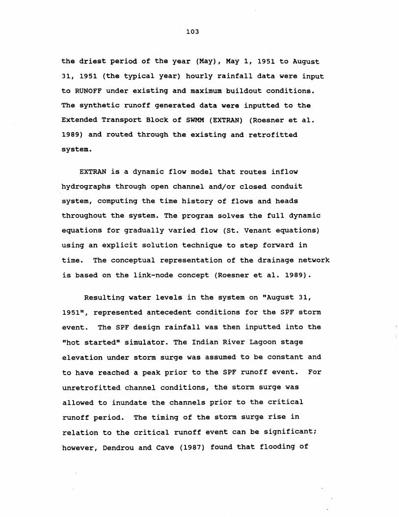
103
the driest period of the year (May), May 1, 1951 to August
31, 1951 (the typical year) hourly rainfall data were input
to RUNOFF under existing and maximum buildout conditions.
The synthetic runoff generated data were inputted to the
Extended Transport Block of SWMM (EXTRAN) (Roesner et ale
1989) and routed through the existing and retrofitted
system.
EXTRAN is a dynamic flow model that routes inflow
hydrographs through open channel and/or closed conduit
system, computing the time history of flows and heads
throughout the system. The program solves the full dynamic
equations for gradually varied flow (st. Venant equations)
using an explicit solution technique to step forward in
time. The conceptual representation of the drainage network
is based on the link-node concept (Roesner et ale 1989).
Resulting water levels in the system on "August 31,
1951", represented antecedent conditions for the SPF storm
event. The SPF design rainfall was then inputted into the
"hot started" simulator. The Indian River Lagoon stage
elevation under storm surge was assumed to be constant and
to have reached a peak prior to the SPF runoff event. For
unretrofitted channel conditions, the storm surge was
allowed to inundate the channels prior to the critical
runoff period. The timing of the storm surge rise in
relation to the critical runoff event can be significant;
however, Dendrou and Cave (1987) found that flooding of

104
coastal catchments in Virginia was relatively insensitive to
the timing of the tide. Using a constant tidal boundary
also eases analysis and adds further margins of safety. A
schematic of the simulator setup is shown in Figure VI-3.
Note that the wetland system was simulated as a wide shallow
trapezoidal channel because of a lack of survey information.
Junction and weir data input to the simulator are summarized
in Table VI-2
TSS Removal Performance in Channel
The use of sedimentation basins and detention basins is
a traditional engineering approach to water pollution
control and peak flow reduction. The theory of
storage/treatment devices has been thoroughly covered by
other (Medina et al., 1981a, 1981b; Goforth, 1981; Nix,
1982; and Nix, 1985) as well as the optimization of their
configurations (Nix et al., 1988 and Nix and Heaney 1988).
McCuen and Moglen (1988) demonstrated how basin geometry can
be manipulated to meet multiple objectives in water
resources management. Many authors have documented the
treatment efficiencies of various basin configurations with
field studies. Unfortunately, few have used their data to
calibrate design methods or deterministic models. For
example, when evaluating a wet detention basin in Central
Florida, Martin (1988) suggested estimates of removal
efficiencies for a number of environmental factors.
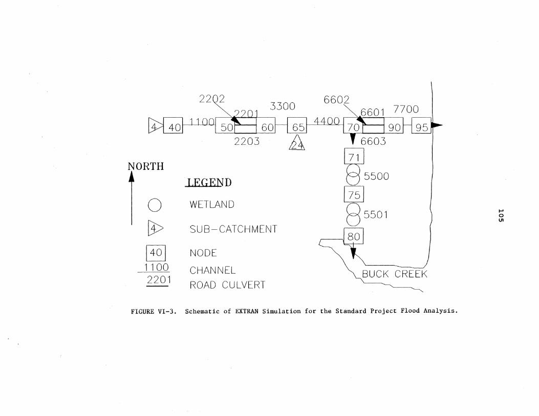
2202 3300 6602
NORTH !
LEGEND
0 WETLAND l I~~~. ~
0 U1 \ I
[9 SUB-CATCHMENT
~ NODE
1100 CHANNEL '\ BUCK CREEK 2201 ROAD CULVERT
FIGURE VI-3. Schematic of EXTRAN Simulation for the Standard Project Flood Analysis.

106
Table VI-2. EXTRAN Junction Data for Standard Project Flood Analysis.
Existing Channel, No Weir:
JUNCTION GROUND CROWN INVERT Qinitial INITIAL NUMBER ELEV. ELEV. ELEV. DEPTH
(ft MSL) (ft MSL) (ft MSL) (cfs) (ft)
40 7.7 6.17 2.1 0.0 1.90 50 7.7 6.00 2.0 0.0 2.00 60 7.7 6.10 1.6 0.0 2.40 65 7.5 5.50 1.0 0.0 3.00 70 5.0 3.80 -0.7 0.0 4.70 90 4.1 4.80 -0.7 0.0 4.70 95 4.1 3.80 -1.7 0.0 5.70
Channel Retrofitted with Weirs:
JUNCTION GROUND CROWN INVERT Qinitial INITIAL NUMBER ELEV. ELEV. ELEV. DEPTH
(ft MSL) (ft MSL) (ft MSL) (cfs) (ft)
40 7.7 6.17 2.17 0.0 0.88 50 7.7 6.00 2.00 0.0 1. 05 60 7.7 6.10 1.60 0.0 1. 45 65 7.5 6.00 1. 00 0.0 2.00 70 5.0 4.50 0.00 0.0 3.05 71 4.1 3.50 2.00 0.0 1. 20 75 4.1 3.50 2.00 0.0 1. 20 80 4.1 3.50 2.00 0.0 1.20
Weir Data:
FROM TO CREST WEIR WEIR JUNCTION JUNCTION HEIGHT TOP LENGTH
(ft MSL) (ft MSL) (ft)
70 71 3.0 5.0 50 70 OUTFALL 4.5 7.5 60 80 OUTFALL 6.2 13.2 6

107
Detention basins are normally categorized as one of
three types: (1) plug flow, (2) completely mixed, and (3)
intermediately mixed. Nearly all basins can be categorized
as intermediately mixed (Nix, 1985), but it is useful to
conceptualize them as one of the two extreme modes in order
to take advantage of simpler mathematics. Detention basins
receive non-steady flows. Theoretically, mean residence
time in a steady-state basin can be described by the
relationship:
(10)
where tr = residence time (hrs.)
V = basin volume (ft.A3), and
Q = hydraulic loading rate (ft. A3/hr.).
However, this simple relationship does not describe the mean
residence time of a detention basin under non-steady state
conditions. This does not preclude, however, the
possibility that the steady state equation may approximate
theory under certain circumstances (Nix, 1985). Long,
rectangular basins where settling is an important removal
mechanism is one case. The proposed weired channel in this
study was represented as a 5500 ft. long, 3 ft. deep
trapezoidal wet detention basin. The proposed side-flow
weir to the wetland system had an invert elevation of +3.0
ft. MSL and a width of 50 feet. Even though the basin had
a very large volume and very long travel path, nearly the

108
entire volume of the basin was dead storage. Relatively
little change in live storage occurred. Therefore, the
steady-state equation may approach the theoretical
approximation.
This study used a deterministic model approach
(storage/Treatment Block of SWMM) supported by site specific
settleability data to evaluate the relative treatment
efficiencies (sedimentation of solids) in the weired trunk
channel. The SIT Block uses the modified PuIs method of
reservoir routing (Viessman et al., 1977) to route flows
through the basin. Pollutants can be routed by one of two
modes: complete mixing or plug-flow. Removal is predicted
with either a user supplied removal equation containing one
or more terms with state variables such as residence time
and inflow concentration, or a discrete particle settling
routine (in the plug-flow mode only).
The hourly runoff flows and TSS loads produced by RUNOFF
were routed through the proposed storage-treatment system
simulated by the SIT Block of SWMM. Outflow from the basin
was determined by a broad-crested weir power equation where
the weir coefficient and power coefficients were assumed to
be 3.33 and 1.5, respectively. The storage basin was
assumed to behave as a completely mixed reactor.
Sedimentation of TSS was represented by the first-order
"reaction" equation developed from site-specific
settleability data (presented in Chapter IV). Although

109
plug-flow conditions combined with typical settling velocity
distribution data may be more applicable to settling of
solids in a very long basin, such a system could not be
simulated with the existing model. An unsuccessful attempt
was made to modify the SIT Block to account for more than
100 plugs within each time step or by reducing the number of
plugs accounted for by increasing the time step. No
reasonable combination was obtained. Removal percentage was
defined as the percent of the solids load entering the basin
that "decay" there.
Groundwater Discharge to Channels
For the coordinated and planned management of both
surface water and groundwater, watershed models must include
detailed groundwater processes with surface water processes.
This significantly increases the complexity of the modeling
effort. As noted in Chapter VI, the subsurface flow
subroutine in RUNOFF is fairly simple in design and contains
numerous parameters to be estimated. However, the
parameters are physically based and some were calibrated to
provide acceptable results. By placing a weir in the trunk
drainage channel, the depth of water in the channels will
rise to approximately the invert elevation of the weir
during dry-weather. This increase of water depth in the
channel can be expected to reduce the subsurface hydraulic

110
gradient to the channel which results in a decrease of
groundwater discharge.
To estimate this reduction after constructing a weir in
the channel, RUNOFF model parameters representing water
depth in the channel were specified to represent the invert
elevation of the outfall weir. For the purposes of
groundwater discharge simulation, these water depths were
assumed to remain constant in the channels. During wet
weather, however, water levels in the channels rise rapidly
(more rapidly than the water table) which, in effect,
minimizes groundwater discharge during wet-weather. This
results in groundwater discharge being primarily a dry
weather and transition between wet and dry weather period
phenomenon. Therefore, assuming a constant channel stage for
groundwater discharge computations provided a reasonable
simulation approach. The prolonged storage of "colored"
groundwater in the channel was assumed not to reduce its
color content even though a dilution affect would occur.
Other Performance Measures
The trunk channel water level elevation was assumed to
remain relatively static near the outfall invert elevation.
Minor fluctuations will occur during wet-weather and
extended dry periods due to evaporation. However dynamic,
seasonal water level variations were assumed to be all but
removed by a retrofitted drainage system. water levels

111
could be manipulated by bleeding down the basin on a
scheduled basis. The determination of a mulitiobjective
water level schedule in the trunk channel was beyond the
scope of this study.
No general guideline criteria for freshwater discharge
to an estuary could be found for the Indian River Lagoon.
Most data and impacts documented are highly site specific"
As a guide in selecting a performance measure, discharge
from subcatchments 4 and 24 under predevelopment conditions
was simulated using RUNOFF (assuming 1% hydraulically
connected impervious area). Under this scenario, no surface
runoff occurred during the "typical" year; all discharge was
accounted by groundwater seepage. Pre-development mean and
maximum discharge were 0.73 and 1.58 cfs, respectively. In
order to compare annual runoff event statistics from various
development scenarios, a common minimum interevent time
(MIT) of 2.0 hours with a baseflow of 1.5 cfs was used to
define runoff events from the hourly time series. Assuming
that the time between runoff events (delta t) is
exponentially distributed, the adequate MIT is the one
leading to a coefficient of variation equal to one for delta
t (Hydroscience, Inc., 1979).
Using common event definitions for the three development
scenarios, the coefficient of variation ranged from 1.1 to
1.3. Distinct characteristic differences in the runoff time
series between the development scenarios accounts for the

112
differing coefficients of variation. The frequency of mean
event flow rates (total event discharge/event duration) for
each development scenario is shown in Figure VI-4. Using
this figure, a mean event freshwater discharge of 5 cfs was
selected as a starting point performance measure for
maintenance of the Indian River Lagoon salinity. Although 5
cfs is in excess of events experienced under pre-
development, it represents a compromise in reaching a
pragmatic goal. Performance of the control system was
determined by inputting the hourly output from the wetland
outfall (represented as a second detention unit in the SIT
Block) into the SWMM statistics Block and summarizing events
based on the common event definition.
Performance Measures Specific to a Wetland System in Florida
The State of Florida Henderson Wetlands Act authorizes
the use of certain wetlands for the treatment of stormwater
and domestic wastewater. The recent Reclaimed Water to
Wetlands Rule provides design criteria for the discharge to
treatment or receiving wetlands. This rule requires
pretreatment for stormwater prior to discharge to the
wetland so as to the protect the ecological balance and
function of the wetland to be used. Efforts were made to
compare performance with design criteria with the most
notable exceptions being the annual average loading
concentration of Total Nitrogen (as N), Total Phosphorus
8
7 -
6 -
1] 5 c Q)
> w
(; 4 'Q)
.0
E ::J
Z 3
2
-
o I I I I
1 1.5 2 2.5 3 3.5 4 4.5 5 5.5 6 6.5 7 7.5 8 8.5 9 9.5 1010.51111.5
Mean Event Flow Rate, cfs
• Pre-development [I] Existing Land Use D Maximum Buildout
Figure VI-4. Frequency of Mean Event Discharge for the "Typical" Year Under Varying Development Scenarios.
......
...... w

114
(as P), and Carbonaceous Biochemical Oxygen Demand (CBOD5).
A comparison of the Ryan and Goetzfried (1988) and Jones
(1986) data on nutrient concentrations in KSC drainage
channels with design criteria suggests that the criteria can
be met, with perhaps the exception of TSS. This comparison
is shown in Table VI-3.
Performance Results
The multiobjective performance of the system is
summarized in Table VI-4. The results suggest that both
the existing and retrofitted systems perform nominally
(serious road crossing inundation did not occur) under SPF
conditions. Although the wetland overflows under all flood
scenarios, this is not considered a failure. These results
suggest that additional flood protection is gained by a weir
in the channel near the outfall as it prevents storm surge
from entering the drainage network resulting in additional
storage capacity during critical runoff periods. The
wetland also provides additional storage. Increasing the
Manning's n friction coefficient of the channel to represent
those typical of heavily vegetated channel (Manning's n of
0.1), resulted in system failure under all scenarios.
Therefore, the system must be continually maintained to
perform under SPF conditions. It is also important to
recognize however, that rainfall data with an hourly time
step may under predict peak flows.

115
Table VI-3. comparison of Untreated Drainaqe water Quality with Wetland Desiqn criteria.
Parameter
TKN
TP
TSS
(1) Mean
Desiqn criteria
3 mq/L
1 mq/L
5 mq/L
for dry weather
Ryan , Goetz fried (1988) (1)
1.3 mq/L
0.27 mq/L
11 mq/L
data at station 5
Jones (1986) (2)
0.6-4.3 mq/L
0.09-1.16 mq/L
4-398 mq/L
near outfall.
(2) wet-weather event composite concentration ranqe.

116
Table VI-4. comparison of Performance for Existing System vs. Retrofitted System.
EXISTING RETROFITTED SYSTEM SYSTEM
EXISTING MAXIMUM EXISTING MAXIMUM lAND USE BUILDOUT lAND USE BUILDOUT
PERFORMANCE MEASURES
Minimum Depth Below Road crossings Under Standard Project Flood 1. 70 ft. 0.00 ft. (1) 2.08 ft. 1.77 ft
Mean Water Depth 0.5 to 0.5 to 3.0 ft. 3.0 ft. in Trunk Channel 1.5 ft. 1.5 ft.
Annual Discharge 588 ac.- 555 ac.- 535 ac.- 516 ac.-of Groundwater feet feet feet feet
Annual TSS Load 272,000 581,000 37,483 121,260 lbs. Ibs. Ibs.(2) Ibs. (3)
Number of Freshwater Discharge Events 42 52 36 39
Number 0 f Mean Freshwater Discharge 6 14 1 8 Events in Excess of 5 cfs.
(1) Road flooding had a duration of one hour.
(2) 86 % removal efficiency.
(3) 79 % removal efficiency.
117
Even though the simulated system meets flood control
criteria, there is uncertainty in some assumptions made.
For instance, what will occur when the wetland overflows has
not been documented. There are parcels of undeveloped
lowlands in that part of the catchment; however, without
survey information, the storage capacity is not known. In
addition, it was assumed that the shoreline dike in the
catchment is continuous, in excess of +4.0 ft. MSL in
elevation, and will prevent storm surge from inundating the
lowland areas of the catchment. Perhaps most importantly is
the question of whether the use of the IDF derived 100yr.-
24hr. storm event occurring simultaneously with the 100-yr.
coastal flood elevation for flood analysis (the joint
probability method) is too stringent and leads to over
designed flood control. Using this traditional civil
engineering design approach has serious consequences in the
design of multiobjective watershed control systems (i.e. the
flood control criteria dominates the design). A better
method would be to analyze historical runoff data, or
synthetic runoff data generated from historical rainfall ,
and receiving water elevations; the flood control design
could then be based on critical "real" storm events. This
method, however, has not made it into the engineering
mainstream primarily because of a lack of sufficient
databases and a general lack of hydrologic analysis
capability in city and facility engineering staffs.

118
Improvements by way of reducing groundwater discharge
are poor. Compromises on flood protection and an aerobic
environment would be required to improve the system. The
model inaccurately represented groundwater discharge under
increasing development scenarios. Rather than representing
groundwater discharge as a function of channel length,
discharge coefficients in the groundwater subroutine in
RUNOFF were developed to represent discharge as a function
of catchment area. Although this approach is not physically
accurate, it is a convenient lumped parameter modeling
method for calibrated catchments. Hindsight has identified
methods to incorporate channel length in the discharge
coefficients (see Appendix C).
Theoretically, wet detention in the weired channel
provides adequate sedimentation that in effect meets The
Stormwater Rule goals of 80% pollutant removal. However,
the criteria for TSS loading to the wetland was not met
which may lead to excessive sedimentation in the wetland.
In addition, scour and resuspension in the channel and the
wetland under extreme storm events was not examined.
Wetlands performance, although not optimal, could be
easily adjusted to provide adequate wetland protection with
additional data and/or additional wetland acres. The
performance of the system with specific respect to the
wetland design criteria is shown in Table VI-5. Detention
time is nearly doubled by raising the outfall invert several

119
Table VI-5. Comparison of Performance for Existing Land Use and Maximum Buildout Specific to Florida Wetland Design criteria.
PERFORMANCE DESIGN EXISTING MEASURE CRITERIA LAND USE
Mean Annual Average TSS Concentration 5 mg/L 16 mg/L
Annual Average Hydraulic Loading 2 - 6 in./wk. 5.1 in./wk. Rate
Minimum Detention 14 days 6 days Time (annual basis)
MAXIMUM BUILDOUT
39 mg/L
6.5 in./wk.
5 days

120
inches; this tradeoff needs to be examined in reducing flow
through the wetland (i.e. primarily mosquito control) and
potential adverse backwater effects in the system. In
addition, the number of high freshwater discharge events and
TSS loads are significantly reduced. The relative
effectiveness in reducing mean freshwater discharge events
for existing land use and maximum buildout is illustrated in
Figures VI-5 and VI-6, respectively.
Cost Analysis
Without performing a complicated and likely
controversial benefit assessment, it was not possible to
quantify the "benefits" and "costs" of a watershed control
system and comparing it to current project specific
stormwater management practices at KSC. However to put the
proposed watershed control program into perspective, cost
analysis was required.
It would be incorrect to directly compare single
objective, site specific project costs with multiobjective
watershed project costs. However, from an operational
decision making standpoint, it is possible to weigh the
current single objective regulatory requirement costs with
an experimental, process-control oriented system that may
take advantage of economies of scale and more efficient O&M
but require more manpower to perform well. It is also

.11 c:
~ a '-<II .0
E ::J Z
.11 c: <II
~ '0 '-<II .0
E :::> z
121
11
10 - Existing Land Use, N = 42 9 - With Watershed Control, N = 36
8 -
7 -
6 -
5 -
4 -
3 -
2 -
o
-
n n n n 1 1.5 2 2.5 3 3.5 4 4.5 5 5.5 6 6.5 7 7.5 8 8.5 9 1010.51111.5
Meon Event Flow Rote. cfs _ Existing Lond Use c:::::J With Control System
Figure VI-5. Frequency of Mean Event Discharge for Non-Control and Watershed Control Under the Existing Land Use Scenario.
8
Maximum Buildout, N - 52 7 With Watershed Control, N - 39
6
5 -
4
3
2 -
1 1.5 2 2.5 3 3.5 4 4.5 5 5.5 6 6.5 7 7.5 8 8.5 9 9.51010.51111.5
Meon Event Flow Rote. cfs _ Moximum Buildout c:::::J With Control System
Figure VI-6. Frequency of Mean Event Discharge for Non-Control and Watershed Control Under the Maximum Buildout Scenario.

122
important to recognize the difficulty in estimating the
number and size of single project basins for the future in a
proposed retrofitted catchment. Several subcatchments may
have to be retrofitted to support a centralized area of
development. For example, the Industrial Area would require
retrofitting projects for three subcatchments. The KSC VAB
area might require retrofitting of as many as four
subcatchment outfalls. Therefore this cost analysis only
represents a typical cost of retrofitting a single "typical"
subcatchment.
The costs in 1989 dollars for the different management
techniques were calculated by estimates provided in the
literature and derived from interviews and multiplying them
by appropriate historical cost factors provided by the 1989
Means Cost System. Cost estimates are shown in Tables VI-6
and VI-7. The typical costs of constructing control
structures for a weired trunk channel with flow through
wetland system was $28,100.00 in 1989 dollars. Assuming
process control and monitoring will be required for the life
of the project, average annual costs were approximated at
$17,100.00/yr. in 1989 dollars.

123
Table VI-6. Cost Analysis for Demonstration Scale Watershed Control System.
Surveying Man Hours Hourly Wage Overhead Multiplier
Cost of Surveying
Design Engineering Engineer Man Hours Technician Man Hou Engineer Wage Technician Wage Overhead Multiplie
Cost of Design Engineering
Permitting Permit Specialist Man Hours Permit Specialist Wage Overhead Multiplier
Cost of Permitting
Control Structure Construction Number of 40,' 30" Corrugated Aluminum Culverts w/ Flap Gates and Adjustable Flow Restrictors Cost of Culvert and Installation Emergency Overflow Weir Construction Side Flow Weir to Wetlands Construction (adjustable)
64 hr. 13 $/hr. 3
2496.00 $
160 hr. 40 hr. 20 $/hr. 10 $/hr. 3
10800.00 $
40 hr. 12 $/hr. 1.2
576.00 $
4 1300 $/culvert 5000 $
4000 $ ------------------------------------------------------------Cost of Control Structure Construction 14200.00 $

124
Table VI-6--continued.
Monitoring Number of Monitoring Stations Number of Years of Monitoring Analytical Cost per tation sampling Man Hours Sampling Technician
5 10 yrs. 1500 $/st/yr. 36 hrs/yr. 8 $/hr.
------------------------------------------------------------Cost of Monitoring
Process Control Number of Years of Controlling Controller Man Hours Controller Wage
Cost of Process Control
Additional operation & Maintenance Number of Years of O&M Number of Pieces of Heavy Equipment Heavy Equipment Operation Cost Crew Size Hourly Wage Time per Man per Year
Cost of Additional Operation & Maintenance
77880.00 $/10 yrs.
10 yrs. 560 hrs./yr. 15 $/hr.
84000.00 $/10 yrs.
10 yrs. 2 equip. 1. 25 $ /hr . / equ. 2 men 10 $/hr. 40 hrs./yr.
9000.00 $/10 yrs.
************************************************************ Estimated Total Project Cost Over 10 Years: 198952 $/10 yrs. ************************************************************

125
Table VI-7. Cost Analysis for Single Project Basins in a Subcatchment.
Design Engineering Engineer Man Hours per Basin Technician Man Hours per Basin Engineer Wage Technician Wage Overhead Multiplier
30 hr. a hr. 20 $/hr. 10 $/hr. 3
------------------------------------------------------------Cost of Design Engineering 2040 .• 00 $/Basin
Permitting Permit Specialist Man Hours per Basin Permit Specialist Wage Overhead Multiplier
Cost of Permitting
Retention/Detention Basin Construction Average Construction Cost per Basi
Cost of Basin Construction per Year
Additional operation & Maintenance Number of Years of O&M Number of Pieces of Heavy Equipment Heavy Equipment Operation Cost Crew Size Hourly Wage Time per Man per Year
Cost of Additional Operation & Maintenance
Fixed Cost per Basin No. of Basins Constructed in 10 Year Period Annual Cost
30 hr. 12 $/hr. 1.2
432.00 $/Basin
30000 $/Basin
30000 $/Basin
10 yrs. 2 equip. 1. 25 $/hr/equ. 2 men 10 $/hr. 64 hrs./yr.
1440.00 $/yr.
32472 $/Basin 5 1440 $/yr.
************************************************************ Estimated Total Project Cost Over 10 Years: 176760 $/10 yrs. ************************************************************


CHAPTER VII
SUMMARY AND CONCLUSIONS
Summary
Evidence documenting the degradation of the Indian
River Lagoon is largely circumstantial. Even so, land
drainage has been identified as a primary factor in the
degradation. Agencies are now considering alternatives to
mitigating these effects such as retrofitting existing
drainage networks in problem areas and implementing a
watershed approach to stormwater management. These water
management problems in the Indian River Lagoon are complex.
Rather than identify additional environmental problems
associated with land drainage in the Indian River Lagoon
basin, this study attempted to evaluate mitigation
alternatives for the problems already identified. It
examined the fundamental premise of stormwater management,
the multiple criteria required for a watershed control
system, and attempted to use simulation experiments to test
various objective concerns and make recommendations for
practical application. In summary, it examined, in detail,
critical technical questions regarding the catchment
126

127
hydrology, channel hydraulics, and the treatment potential
of the existing drainage system.
The results of this study include:
1) A literature review of receiving water effects
near KSC.
2) The identification of issues and philosophies
related to water resources management at KSC.
3) Identification of watershed management
objectives and those competing in the Indian
River Lagoon Basin near Merritt Island.
4) Critique of previous watershed modeling
efforts conducted in the Indian River Lagoon
Basin.
5) Collection of site specific hydrologic data
for model calibration.
6) Calibration of SWMM, and with it,
demonstrated cause and effect relationships
in the generation of runoff and TSS loads to
the receiving water.
7) Examined the conjunctive use application of
modeling with SWMM.
8) Preliminary screening of water management
approaches for KSC-wide application.
9) Complete description of the physical layout of
a proposed watershed control system.

128
10) Simulation of the relative effectiveness of
the watershed control system.
11) A cost analysis of the proposed watershed
system versus the current stormwater
management approach.
Negative contributions to the Indian River Lagoon that
are associated with land drainage runoff include nutrients,
muck, "colored" groundwater, excessive freshwater, suspended
solids, and various toxins and pathogens. In an effort to
address these problems, the use of watershed models are
expected to increase significantly.
Environmental management perspectives of stormwater
runoff range from risk aversion to cost-effective approaches
(cost-benefit). While risk aversion is economically
infeasible, the cost-benefit approach is difficult to apply
due to the lack of data on benefits. Florida is considered
a leader in stormwater management regulation in the nation.
Its Stormwater Rule is based on static controls to achieve
cost-effective performance. Several problems remain (e.g.
piecemeal approach can lead to combined effects, lack of
long-term performance data, poor system performance in
Florida Flatwood areas, and a lack of retrofitting of
existing drainage networks) .
The study area was a typical "developed" catchment at
KSC that is 1900 acres in area. It can be described as a

129
Florida Flatwood watershed that has been "improved" with an
extensive drainage network of open channels that were
designed to pass the Standa,rd Project Flood. . It has two
major outfalls to the Banana River portion (Planning Segment
B2) of the Indian River Lagoon. Approximately 350 acres or
18% of the catchment is impervious. The depth to the water
table ranges from 2.5 to 4.5 feet below the land surface.
Segment B2 is not influenced by astronomical tide but does
undergo quasi-periodic fluctuation due to aeolian tide or
wind setup. This phenomenon causes reversible flow and
backwater effects in the channels near the outfalls during
dry weather.
Objectives of an ideal control system were identified as
(1) flood protection, (2) reduce groundwater discharges, (3)
reduce pollutant loads, (4) maintain an aerobic environment
in the channel waters and sediments, (5) reduce extreme
freshwater discharge events, (6) . enhance the littoral
habitat of the channels, and (7) prevent mosquito
infestation. Measures of performance for each objective
were then developed based on regulatory guidelines and
literature suggestions. using a simple decision-aiding
matrix (primarily based on the Cardinal utility), nine
potential control systems were screened. The option of
channel retrofitting with wetland routing was selected as
most likely to provide the best overall system performance.

130
The study area lacked an appropriate database;
therefore, ten months of site-specific data on
precipitation, water stage, water table elevation, channel
water velocity, event mean concentration of TSS loads, and
TSS settleability were collected. In addition, urban and
drainage features were added to the KSC GIS. with these
data, the cause and effect relationships of the catchment
hydrology, channel hydraulics, and pollutant loads were
documented and summarized using the calibration and
verification of the SWMM model. The simulation included
groundwater discharge to the channels. The surrogate
pollutant, TSS, was best represented by a rating curve to
describe scour in the drainage channels. The generation of
runoff was most sensitive to the depth to the water table,
catchment width, and percent imperviousness.
This calibrated model was then used to estimate
"typical" loadings to the estuary. This was performed by
running a continuous simulation of the RUNOFF block of SWMM
with a "typical" year (1951) of hourly rainfall data. For
the estimates it was assumed that no TSS removal occurred in
the trunk channels. Yearly loadings were estimated for both
existing land use and the maximum buildout scenario. The
model estimated that annual freshwater discharge would
increase by 18% and annual TSS loads increase by 290%.
The calibrated model was then used to evaluate the
relative effectiveness of the proposed watershed control

131
system under existing land use and maximum buildout. The
feasibility of the proposed system was evaluated in detail
for only one of the outfalls of the study area. The
proposed demonstration scale project involves constructing
three adjustable water control structures and connecting a
partially disturbed interdunal swale freshwater wetland site
to the drainage network. Two weir control structures are
proposed near the outfall of the trunk channel; one
functions as an emergency spillway discharging directly to
the estuary and the other, a side-spill weir, routes dry and
wet-weather flows through the forty acre wetland site.
Discharge from the wetland will be controlled by a series of
adjustable, flap-gated culverts. The trunk channel will
provide primary sedimentation as a wet detention basin and
the expected function of the wetland system is to provide
nutrient assimilation, additional storage, and enhanced
evapotranspiration.
The system was then evaluated using the general
objectives and objectives specific to the wetland system
established by the regulatory agencies. Even though the
system was not optimized due to analytical uncertainty, it
was apparent from the simUlation experiments that the system
could not satisfy all of the objectives. without sufficient
scientific evidence documenting the importance of individual
factors contributing to the degradation of the Indian River
Lagoon, it would be erroneous to prioritize the various
water quality improvement objectives. with SPF based flood

132
control as a pre-emptive goal, the simulated system only
achieved nominal performance for flood control, TSS load
reduction, and maximum water depth. Long-term performance
of the wetland system could not be predicted; however, it
will likely result in the reduction of dissolved water
quality constituents.
The simulation experiments clearly illustrated that th$
system will have great difficulty in meeting the groundwater
discharge and water level fluctuation criteria under all
development scenarios. Without periodic drawdown, water
levels in the system will be near static. Groundwater
discharge was estimated to be reduced only 9%. Under
maximum buildout, sedimentation in the wetland may be a
problem. Improvements in reducing the number of freshwater
discharge events in excess of the criteria are made;
however, numerous failures were recorded under maximum
buildout. To improve overall performance, this work
suggests that further compromises in the objectives will be
required as well as collecting actual system performance
data. This will involve critiquing the scientific basis of
the criteria, in particular the justification of using
synthetic design storms for flood control design and the
measurement of actual TSS loads to the wetland.
An itemized cost analysis determined that the fixed
cost of the proposed system would be approximately
$28,072.00 in 1989 dollars. Annual process control and

133
monitoring costs were estimated to cost $17,088.00 per year.
Over a ten year life of the project, the cost would be
expected to be $198,953.00 in 1989 dollars. Based on
construction trends since 1984, it was estimated that the
construction of individual project stormwater basins for the
demonstration subcatchment would cost $176,760.00 over ten
years in 1989 dollars. The cost of constructing a typical
retention basin was estimated from previous KSC construction
to be approximately $30,000.00. Although it would be
incorrect to directly compare single objective, site
specific project costs with multiobjective watershed control -
project costs, such a comparison illustrates that the
proposed system would not only be expected to be more
effective in addressing receiving water quality issues but
cost competitive as well.
Conclusions
To address receiving water effects in the Indian River
Lagoon, stormwater management on the watershed scale must
take on a multiobjective analysis approach. As this study
highlights, addressing the multiobjective criteria required
to design a watershed control system is no trivial endeavor.
From a practical standpoint, all of the criteria can not be
optimally achieved which raises some very interesting
tradeoff questions. For example, can a portion of the flood
protection margin of safety be traded for expected

134
improvements of water quality? Do the expected benefits of
water quality improvements due to an untested flow-through
wetland treatment system compensate for utilizing the
wetland resource? Although costs would be expected to be
comparable to current management practices, performance
would certainly be enhanced. optimization and justification
of such systems can not be made until adequate· receiving
water analyses are conducted.
The flood protection performance of the system is very
sensitive to the height of vegetation in the channels. This
study suggests that channels must be maintained regularly.
However, data from this study also support the hypothesis
that the regular denudation of vegetation in the channel
results in a significant contribution to the TSS load from
the catchment. Where practical, it is recommended that
channel vegetation be maintained by methods other than
scraping and removal of sod (e.g·. mowing or clipping during
dry weather). periodically the wetland system may require
maintenance to reduce organic matter accumulation, remove
accumulated sediment, and reduce the buildup of hillocks
which encourage channelization of flow, Case studies show
that burning, water level drawdown, and scraping are
commonly used for wetland maintenance. By reducing TSS
production due to channel scour, wetland sedimentation is
not expected to be a problem. Therefore, periodic burning
and water level drawdown may prove to be sufficient wetland

135
maintenance. This subject is covered in more detail by
others (Hyde et ale 1984; USEPA, 1988).
A number of recommendations can be made with respect to
the application of SWMM to additional watershed analysis in
the Indian River Lagoon Basin. A variable time step option
is available in RUNOFF (found in the B3 card); however,
other modules of SWMM do not have such an option which leads
to problems in coupling RUNOFF with other SWMM modules (e.g.
large continuity differences between the modules). A
constant time step is recommended if RUNOFF output is to be
interfaced with other SWMM modules. The groundwater
subroutine in SWMM is simple yet semi-physically based. For
future applications to surface-subsurface water management
it is recommended that groundwater discharge coefficients be
developed to represent seepage face length (channel length)
rather than catchment area. Also, as the SWMM manual notes,
this subroutine does not account for exfiltration from the
channel. This was found to be significant in this study,
particularly during dry weather. A nice review of transient
seepage can be found in Bouwer (1978). For evaluation and
design, plug flow best represents the wet detention in the
retrofitted channels. However without major modification of
the model (SIT Block), it is not possible to continuously
simulate plug flow in these lengthy channels. If model
modification is avoided, one option would be to develop and
utilize a historical design storm time series of pollutant

136
load for predicting the relative treatment effectiveness of
the retrofitted channel.
Although an estimate of the settleability of TSS in the
stormwater effluent was provided in this study, certainly
additional effluent treatability study is warranted.
Information on the settleability of nutrients, metals, and
hydrocarbons would help "fine tune" the proposed system.
The establishment of a long-term lagoon water level data
base would be beneficial to future water resources analysis
and design and estuarine research. Mathematical models of
seagrass systems offer an interesting new approach to
receiving water analysis. The feasibility of incorporating
such models into environmental management (i.e. used as an
all encompassing measure of system performance) should be
investigated.
Hydrologic simulation is a very powerful technique in
organizing and understanding the catchment hydrology and
hydraulics and in examining the relative effectiveness of
management scenarios. However, this detailed analysis has
highlighted that due to the analytical uncertainty, system
performance can only be optimized through dynamic designs
supported by dynamic simulation. As Schilling (1985)
concludes in his excellent overview of real-time control of
urban runoff quality management,

137
"There is no need for further research into even
more involved mathematical techniques,
but there is a great need for •.. joint
research/application projects and enhanced
communications between scientists, engineers, and
operators."
Perhaps the time has come for the implementation of
experimental, dynamic watershed control systems to address
the multiple water management objectives in the Indian River
Lagoon Basin.

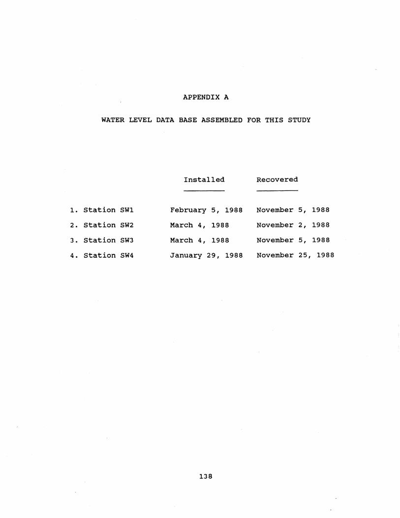
APPENDIX A
WATER LEVEL DATA BASE ASSEMBLED FOR THIS STUDY
1. station SW1
2. Station SW2
3. Station SW3
4. station SW4
Installed
February 5, 1988
March 4, 1988
March 4, 1988
January 29, 1988
138
Recovered
November 5, 1988
November 2, 1988
November 5, 1988
November 25, 1988


APPENDIX B
LISTING OF SWMM INPUT FILES FOR THE RUNOFF BLOCK FOR THE STUDY AREA UNDER EXISTING LAND USE AND MAXIMUM BUILDOUT

* KSC STORMWATER MANAGEMENT
* * DREW B. BENNETT, UNIVERSITY OF FLORIDA
* * INPUT FILE FOR RUNOFF BLOCK ************************************************.****************************
* CONTINUOUS SIMULATION FOR INDUSTRIAL AREA: 1951: CALC QUALITY & TSS LOAD * ***************************************************************************** * PREDICTION OF RUNOFF AND TSS LOAD UNDER EXISTING LAND USE * .********************************************************.*.*****************
SW 8 25 MM 7 9 12 13 14 15 16 17 a 9 'STMET51.0UT' a 25 'INDRO.INT' SRUNOFF A1 'RUNOFF FOR INDUSTRIAL AREA' A2 'SIX SUB-CATCMENTS, 1900.5 ACRES'
* B1 B2 B3 B4
* D 1
*
o o 900.0
30.0
o 0 o 2 3600.0 7200.0
0.01 2
o 51
8760
F1 0.09 0.12 0.18 0.22 0.24 0.22 0.21 0.21 0.21 0.19 0.17 0.11 0.08
* G1 444 60 G2 0 0.04 G1 244 60 G2 0 0.0 G1 555 10 G2 o 0.04 G 1 155 10 G2 o 0.04 G1 111 10 G2 0 0.0 G 1 333 10 G2 o 0.04
* H 1
H2 4 4 444
444
5 15 4000 0.00035 2 2 0.044 4
3.3 3 5 15 6000 0.00046 2 2 0.04 4
3.3 3 5 15 4000 0.0001 2 2 0.04 4
3.3 3 5 15 5600 0.0004 2 2 0.04 4
3.3 3 5 15 6200 0.0001 2 2 0.08 4
3.3 3 5 15 4000 0.0004 2 2 0.04 4
3.3 3
4000 167 18 0.00012 0.0
0.013 0.25 0.05 0.4 10 1 .8 8.0 4.5
H3 1.2E-4 2.0 0 1.2E-4 0.3 0.03 0.05 5.0 0.001 0.00003 4.5
0.035
H4 10 15
* H 1 H2 H3 H4
*
24 24 1.2E-4
10
244 244 2.0
15
7640 1
o
316
1.2E-4 0.001
5 0.00012 0.013 0.25 0.0 5.0 3.8
0.3 0.03 0.05 0.00003 4.5
5.0
0.05 0.4 10 0.0
0.035
0.1
1 .0
0.0
o • 1
1.5
0.1
5 0.00115 - 1 .0
5 0.00115 2.9
H 1
H2 H3 H4
1 5
5 1.2E-4
555 3000 555
133 15 0.000012 0.013 0.0 8.0 4.5
0.25 0.05 0.4 10 5 0.00115 4.7 -1.0
2.0 0 10 15
1.2E-4 0.3 0.03 0.05 0.001 0.00003 4.5
140
5.0 0.035
141
* H 1 1 3 333 4000 489 4.5 0.000012 0.013 0.25 0.05 0.4 10 5 0.00115 H2 3 333 1 0.0 5.0 3.8 3.8 - 1 .0 H3 1.2E-4 2.0 0 1.2E-4 0.3 0.03 0.05 5.0 0.035 H4 10 15 0.001 0.00003 4.5
* H 1 111 6300 577 0.0 0.000012 0.013 0.25 0.05 0.4 10 5 0.00115 H2 111 0.0 8.0 4.5 3.0 1 .5 H3 1.2E-4 2.0 0 1.2E-4 0.3 0.03 0.05 5.0 0.035 H4 10 15 0.001 0.00003 4.5
* H 1 15 155 3600 218.5 15 0.000012 0.013 o . 25 0.05 0.4 10 5 0.00115 H2 15 155 1 o . 0 8.0 4.5 1 .8 - 1 . 0 H3 1.2E-4 2.0 0 1.2E-4 0.3 0.03 0.05 5.0 0.035 H4 10 15 0.001 0.00003 4.5
* J 1 0 0 4.0 0.0 1 .0 0.0 0.0 0.0 367
* J2 'GENERAL' 0 0 10000 1 .0 5.0 o . 0 0.0 0.0 J3 ' T S S ' 'MG/L' 0 0 0 0 100000 1.0 5 0.0 0.0 1 • 1 5 40 0.0 0.0 0.0 J4 0 0 0.0
* L 1 1 0 0/ L 1 3 0 66 0/ L 1 4 0 138 0/ L 1 5 0 87 01 L 1 15 0 102 01 l1 24 0 40 01
* MO 1 .0 M1 2 0 M2 0 0 M3 10 60 SEND PROGRAM

142
* KSC STORMWATER ~ANAGEMENT
* * DREW B. BENNETT, UNIVERSITY OF FLORIDA
* * INPUT FILE FOR RUNOFF BLOCK ***************************************************************************** * CONTINUOUS SIMULATION FOR INDUSTRIAL AREA: 1951: CALC QUALITY & TSS LOAD * **************.****.****.********************************************* •• **.*. * PREDICTION OF RUNOFF AND TSS LOAD UNDER MAXIMUM BUILDOUT *********************.*.*******.***** ••• *************************************
SW 1 8 25 MM 7 9 12 13 14 15 16 17 iii 9 'STMET51.0UT' iii 25 ' INDRO.INT' $RUNOFF A1 'RUNOFF FOR INDUSTRIAL AREA' A2 'SIX SUB·CATCMENTS, 1900.5 ACRES' * B1 0 0 0 0 51 B2 0 0 2 B3 900.0 3600.0 7200.0 2 8760 B4 30.0 0.01 * 01 *
F 1 0.09 0.12 0.18 0.22 0.24 0.22 o . 21 0.21 0.21 0.19 0.17 0.11 0.08
* G1 444 60 5 15 4000 0.00035 2 2 0.044 4 0.1
G2 0 0.04 3.3 3 G1 244 60 5 15 6000 0.00046 2 2 0.04 4 1 .0
G2 0 0.0 3.3 3
G1 555 10 5 15 4000 0.0001 2 2 0.04 4 0.0
G2 0 0.04 3.3 3
G1 155 10 5 15 5600 0.0004 2 2 0.04 4 0.1
G2 0 0.04 3.3 3 G1 11 1 10 5 15 9000 0.0001 2 2 0.08 4 1.5
G2 0 0.0 3.3 3 G1 333 10 5 15 5000 0.0004 2 2 0.04 4 0.1
G2 0 0.04 3.3 3
* * * * H 1 4 444 4000 167 18 0.00012 0.013 0.25 0.05 0.4 10 5 0.00115
H2 4 444 1 0.0 8.0 4.5 1.8 - 1 .0
H3 1.2E-4 2.0 0 1.2E-4 0.3 0.03 0.05 5.0 0.035
H4 10 15 0.001 0.00003 4.5
* H 1 24 244 7640 316 18 0.00012 0.013 0.25 0.05 0.4 10 5 0.00115
H2 24 244 0.0 5.0 3.8 0.0 2.9
H3 1.2E-4 2.0 0 1.2E-4 0.3 0.03 0.05 5.0 0.035
H4 10 15 0.001 0.00003 4.5

143
* H1 5 555 3000 133 18 0.000012 0.013 0.25 0.05 0.4 10 5 0.00115 H2 5 555 1 0.0 8.0 4.5 4.7 -1.0 H3 1.2E-4 2.0 0 1.2E-4 0.3 0.03 0.05 5.0 0.035 H4 10 15 0.001 0.00003 4.5
* H1 3 333 4000 489 18 0.000012 0.013 0.25 0.05 0.4 10 5 0.00115 H2 3 333 1 0.0 5.0 3.8 3.8 - 1 .0 H3 1.2E-4 2.0 0 1.2E-4 0.3 0.03 0.05 5.0 0.035 H4 10 15 0.001 0.00003 4.5
* H1 111 6300 577 18 0.000012 0.013 0.25 0.05 0.4 10 5 0.00115 H2 111 1 0.0 8.0 4.5 3.0 1 .5 H3 1.2E-4 2.0 0 1.2E-4 0.3 0.03 0.05 5.0 0.035 H4 10 15 0.001 0.00003 4.5
* H 1 15 155 3600 218.5 18 0.000012 0.013 0.25 0.05 0.4 10 5 0.00115 H2 15 155 0.0 8.0 4.5 1.8 -1.0 H3 1.2E-4 2.0 0 1.2E-4 0.3 0.03 0.05 5.0 0.035 H4 10 15 0.001 0.00003 4.5
* J 1 0 0 4.0 0.0 1 .0 0.0 0.0 0.0 367 J2 'GENERAL' 0 0 10000 1.0 5.0 0.0 0.0 0.0 J3 ' T S S' 'MG/L' 0 1 0 0 0 100000 1.0 5 0.0 0.0 1 • 1 5 40 0.0 0.0 0.0 J4 0 0 0.0
* * L1 0 429 01 L1 3 0 273 01 L 1 4 0 138 01 L 1 5 0 87 01 L1 15 0 102 01 L1 24 0 210 01
* MO 1 .0 M1 2 0 M2 0 0 M3 10 60 SEND PROGRAM

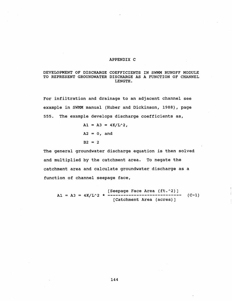
APPENDIX C
DEVELOPMENT OF DISCHARGE COEFFICIENTS IN SWMM RUNOFF MODULE TO REPRESENT GROUNDWATER DISCHARGE AS A FUNCTION OF CHANNEL
LENGTH.
For infiltration and drainage to an adjacent channel see
example in SWMM manual (Huber and Dickinson, 1988), page
555. The example develops discharge coefficients as,
A1 = A3 = 4K/LA2,
A2 = 0, and
B2 = 2
The general groundwater discharge equation is then solved
and multiplied by the catchment area. To negate the
catchment area and calculate groundwater discharge as a
function of channel seepage face,
[Seepage Face Area (ft. A 2)] A1 = A3 = 4K/LA2 * (C-1)
[Catchment Area (acres)]
144

REFERENCES
Bartleson, R.D. The Relative Influence of Current Reduction by Seagrasses on Sediment Nutrients and Seagrass Growth in High and Low Nutrient Waters: A Simulation Model and Field Observations. M.S. Thesis, Univ. of Florida, Gainesville, 1988.
Bedient, P.B. and W.C. Huber. Hydrology and Floodplain Analysis. Addison-Wesley Publishing Company, Reading, MA. 1988.
Bennett, D.B. Analysis and Prediction of Shallow Groundwater Level Behavior in Merritt Island, Florida. Unpublished, special project in environmental engineering. Univ. of Florida, Gainesville. 1988.
Black, A.P. and R.F. Christman. Characteristics of Colored Surface Waters. Jour. AWWA, Vo. 55, No.6, 753-770, 1963.
Bouwer, H. Groundwater Hydrology. McGraw-Hill Book Company, New York. 1978.
Brevard County 208 Areawide Waste Treatment Management Plan. Brevard County Department of Natural Resources, Merritt Island, Florida, February 1979.
Capece, J.C., J.C. Campbell, and L.B. Baldwin. Estimating Peak Rates and Volumes from Flat, High Water Table Watersheds. Paper No. 84-2020, ASAE, st. Joseph, MI, June 1984.
Carlisle, V.W., M.E. Collins, F. Sodek, III, and L.C. Hammond. Characterization Data for Selected Florida Soils. Soil Science Research Report No. 85-1, Dept. of Soil Science, Univ. of Florida, Gainesville. 1985.
Carter, H.H. and Okubo, A. A Study of the Physical Processes of Movement and Dispersion in the Cape Kennedy Area. Report No. NYO-2973-1, Chesapeake Bay Institute Ref. 65-2. 1965.
Christensen, B.A. Hydraulics of Sheet Flow in Wetlands. Proc. 3rd Annual Sympos. of Waterways, Harbors, and Coastal Eng. Div., ASCE, RIVERS 76, Vol. 1, 746-756, Fort Collins, CO, 1976.
145

146
Christensen, B.A. Hydraulic Notes. Hydraulic Laboratory, Dept. of civil Eng., Univ. of Florida, Gainesville, 1985.
Clark Engineers-scientists, Inc. KSC Subsurface Hydrology and Groundwater Survey. The Site Specific Program Report, Miami, Florida, 1985.
Clark Engineers-Scientists, Inc. KSC Subsurface Hydrology and Groundwater Survey. Volume IV, The Areawide Program. NASA Pub. No. KSC-DF-3081. 1987.
Da Costa, S.L. and K.A. Glatzel. Simulating Nonpoint Source Runoff to Coastal Waters. ASCE, Proc. 5th Sympos. Coastal and Ocean Mgmt, Vol. IV, Seattle, Washington, 3903-3916, May 1987.
Delfino, J.J., D. Frazier, and J. Nepshinsky. Contaminants in Florida's Coastal Zone. Florida Sea Grant College Report No. 62. Gainesville, 1984.
Dendrou, S. and K.A. Cave. Accounting for Tidal Flooding in Developing Urban Stormwater Management Master Plans. Proc. of Stormwater and Water Quality Model Users Group Meeting, EPA/600/9-87/016, March 23-24, Denver, CO., 1987.
Diniz, E.V. and W.H. Espey, Jr. Maximum utilization of Water Resources in a Planned Community. Application of the Storm Water Management Model, Volume I. EPA-600/2-79-050c, U.S. Environmental Protection Agency, Cincinnati, OH. July 1979.
Dreschel, T.W. B.C. Madsen, L.A. Maull, C.R. Hinkle, W.M. Knott. Precipitation Chemistry: Atmospheric Loadings to the Surface Waters of the Indian River Lagoon by Rainfall. In press, Florida Scientist.
Driscoll, E.D. In: Benefit Analysis for Combined Sewer Overflow Control. Seminar Pub. EPA-625/4-79-013, Environmental Protection Agency, Cincinnati, OH. April 1979.
Dunne, T. and L.B. Leopold. Water in Environmental Planning. W.H. Freeman and Co., San Francisco, CA. 1978.
Dwornik, D.S. A Stormwater Collection and Reuse System for the Kennedy Space Center. Florida Water Resources Research Center Pub. No. 83, University of Florida, Gainesville, 1984.

147
Ferrara, R.A. and P. Witkowski. stormwater Quality Characteristics in Detention Basins. Proc. ASCE, J. Env. Eng. Div., Vol. 109, No.2, 428-447, 1983.
Florida Department of Regulation. Biological Potential for Slowing, stopping, and Reversing the Trend of Seagrass Loss. Seagrass Task Force "White Paper", Unpublished Report, 1987.
Florida Department of Transportation. Drainage Manual. Florida Department of Transportation, Tallahassee, Florida, 1987.
Fonseca, M.S., W.J. Kenworthy, and G.W. Thayer. Restoration and Management of Seagrass Systems: A Review. Proc. International symposium on Ecology and Management of Wetlands, College of Charleston, Charleston, S.C., June 1986.
Goforth, G.F. Long-Term Performance of Stormwater Detention Facilities: A Comparison of Design Methodologies. Florida Water Resources Research Center Pub. No. 58, University of Florida, Gainesville, 1981.
Grizzard, T.J., C.W. Randall, B.L. Weand, and K.L. Ellis. Effectiveness of Extended Detention Ponds. Proc. Eng. Found. Conf. on Urban Runoff Quality, ASCE, New England College, Henniker, New Hampshire, 323-337, June 1986.
Heaney, J.P. Introduction. In: Introduction to Social Choice Theory for Environmental Decision Making. P.O. Straffin. ASCE Urban Water Resources Reserach Program Tech. Memo. No. 36, February 1979, New York.
Heaney, J.P. Cost-Effectiveness and Urban Storm-Water Quality criteria. Proc. ASCE Conf. on Current Practice and Design criteria for Urban Runoff Water Quality Control, New York. 1988.
Heaney, J.P., W.C. Huber, W.C. Downs, M.C. Hancock, and C.N. Hicks. Impacts of Development on the Water Resources of Cypress Creek, North of Tampa. Pub. No. 89, Florida Water Resources Research Center, Gainesville. 1986.
Heaney, J.P., W.C. Huber, R. Field, and R.H. Sullivan. Nationwide Cost of controlling Combined Sewer Overflows and Urban Stormwater Discharges. Jour. Water Pollution Control Fed., Vol. 51, No.8, Aug. 1979.
Heaney, J.P., W.C. Huber, and M.E. Lehman. Nationwide Assessment of Receiving Water Impacts from Urban Stormwater Pollution. Vo1s. I and II, EPA-600j52-81-025, Cincinnati, OH, 1981.

148
Heaney, J.P., B. Koopman, D.S. Dwornik, and R. Saliwinchik. water Resources of the Kennedy Space Center. Florida water Resources Research Center Pub. No. 82, Univ. of Florida, Gainesville. 1984.
Heffernan, J.J. and R.A. Gibson. A Comparison of Primary Production Rates in Indian River, Florida Seagrass Systems. Florida Scientist, Vol. 46, No. 3/4, 1983.
Holler, J.D. Storm Water Detention Basin Nutrient Removal Efficiency. Proc. ASCE, J. water Resources Planning and Management, Vol. 115, No.1, 52-63, 1989.
Huber, W.C. Deterministic Modeling of Urban Runoff Quality. In: Urban Runoff Pollution. H. Torno, J. Marsalek, and M. Desbordes, eds., NATO ASI Series, Series G: Ecological Sciences, Vol. 10, Springer-verlag, New York, 167-242, 1985.
Huber, W.C. and R.E. Dickinson. Storm Water Management Model, Version 4. Office of Research and Development, U.S. Environmental Protection Agency, Athens, GA., 1988.
Huckle, H.F., H.D. Dollar, and R.F. Pendelton. Soil Survey of Brevard County, Florida. U.S. Department of Agriculture, Soil Conservation Service, Washington, D.C. 1974.
Hyde, H.C., R.S. Ross, and F. Demgen. Technology Assessment of Wetlands for Municipal Wastewater Treatment. USEPA, EPA-600/2-84-154, Office of Research and Development, Cincinnati, OH, 1984.
Hydroscience, Inc. A Statistical Method for Assessment of Urban Stormwater Loads-Impacts-Controls. U.s. Environmental Protection Agency, EPA 440/3-79-093, washington, D.C., 1979.
James, W. and S. Boregowda. continuous Mass-Balance of Pollutant Build-Up Processes. In: Urban Runoff Pollution. H. Torno, J. Marsalek, and M. Desbordes, eds., NATO ASI Series, Series G: Ecological Sciences, Vol. 10, Springer-Verlag, New York, 243-271, 1985.
Jewell, T.K., T.J. Nunno, and D.O. Adrian. Methodology for Calibrating Stormwater Models. Proc. ASCE, J. Env. Eng. Div., Vol. 104, No. EE3, 485-501, 1978.
Jones, K.L. Quantitative Assessment of Stormwater Runoff from the Vehicle Assembly Building Area of Kennedy Space Center, Florida. Master's Thesis, Florida Institute of Technology,' Melbourne, 1986.

149
Laster, J.A. Water Chemistry Studies of the Indian River Lagoons. Report to NASA in An Ecological Study of the Lagoons Surrounding the John F. Kennedy Space Center, Florida. Florida Institute of Technology, Melbourne. 1975.
Levenspiel, o. Chemical Reaction Engineering. Second Edition. John Wiley and Sons, Inc., New York, New York, 1972.
Livingston, E.H. Stormwater Regulatory Program in Florida. Proc. Eng. Found. Conf. on Urban Runoff Quality, ASCE, New England College, Henniker, New Hampshire, 249-256, June 1986.
Manahan, S.E. Environmental Chemistry. Fourth Edition. Willard Grant Press, Boston, 1984.
Martin, E.H. Effectiveness of an Urban Runoff Detention Pond-Wetlands System. Proc. ASCE, J. Env. Eng. Div., Vol. 114, No.4, 810-827, 1988.
McCuen, R.H. and G.E. Moglen. Multicriterion Stormwater Management Methods. Proc. ASCE, J. Water Resour.Plan. and Mgmt., Vol. 114, No.4, 414-431, 1988.
Medina, M.A., W.C. Huber, and J.P. Heaney. Modeling Stormwater Storage/Treatment Transients: Theory. Proc. ASeE, J. Env. Eng. Div., Vol. 107, No. EE4, 1981a.
Medina, M.A., W.C. Huber, and J.P. Heaney. Modeling Stormwater Storage/Treatment Transients: Applications. Proc. ASCE, J. Env. Eng. Div., Vol. 107, No. EE4, 1981b.
Mion, L.P.O. Low-Energy Wastewater Recycling Through an Oligohaline Coastal Marsh Ecosystem. M.S. Thesis, Univ. of Florida, Gainesville, 1986.
Mote Marine Laboratory. Biological and Chemical Studies on the Impact of Stormwater Runoff Upon the Biological Community of the Hillsborough River, Tampa. Final Research Report submitted to Department of Public Works, Tampa, Florida. Mote Marine Laboratory, Sarasota, Florida. 1984.
National Aeronautics and Space Administration. Environmental Resources Document, John F. Kennedy Space Center, Florida, NASA Pub. No. KSC-DF-3080, 1986.
National Oceanic and Atmospheric Administration. Flood Insurance Study, Brevard County, Florida, 1971. '

150
Nix, S.J. Analysis of storage/Release Systems in Urban stormwater Quality Management. Ph.D., Dissertation. Univ. of Florida, Gainesville, 1982.
Nix, S.J. Residence Time in Stormwater Detention Basins. Proc. ASCE, J. Env. Eng. Div., Vol. 111, No.1, 95-100, 1985.
Nix, S.J. and J.P. Heaney. optimization of storm water Storage-Release strategies. Water Resour. Res., Vol. 24, No. 11, 1831-1838, 1988.
Nix, S.J., J.P. Heaney, and W.C. Huber. Suspended Solids Removal in Detention Basins. Proc. ASCE, J. Env. Eng. Div., Vol. 114. No.6, 1331-1341, 1988.
Odum, W.E. and M.E. Hawley. Impacts of Urban Runoff on Estuarine Ecosytems. Proc. Eng. Found. Conf. on Urban Runoff Quality, ASCE, New England College, Henniker, New Hampshire, 182-191, June 1986.
Peffer, S.D. Sediments. Report to NASA in An Ecological Study of the Lagoons Surrounding the John F. Kennedy Space Center, Florida. Florida Institute of Technology, Melbourne. 1975.
Petryk, S. and G. Bosmajian. Analysis of Flow Through Vegetation, Proc. ASCE. J. Hydraulics Div., Vol. 101, No. HY7, 871-884, 1975.
Provancha, J.A. and R.M. Willard. Submerged Aquatic Vegetation Density Classes, John F. Kennedy Space Center, Florida. GIS Information, NASA/KSC Biomedical operations and Research Office, 1986.
Provancha, M.J. P.A. Schmalzer, and C.R. Hinkle. Vegetation Types, John F. Kennedy Space Center. GIS Information, NASA/KSC Biomedical Operations and Research Office, 1986.
Rice, J.D., R.P. Trocine and G.N. Wells. Factors Influencing Seagrass Ecology in The Indian River Lagoon. Florida scientist, Vol. 46, No. 3/4, 1983.
Roesner, L.A., J.A. Aldrich, and R.E. Dickinson. Storm Water Management Model User's Manual Version 4: EXTRAN Addendum. Office of Research and Development, U.S. Environmental Protection Agency, Athens, GA., 1989.
Ryan, J. and A. Goetzfried. Unpublished water quality data for the Buck Creek drainage network. NASA Environmental Management Staff, Design Engineering, John F. Kennedy Space Center, Florida, 1988.

151
Schilling, W. Urban Runoff Quality Management by Real-Time control. In: Urban Runoff Pollution. H. Torno, J. Marsalek, and M. Desbordes, eds., NATO ASI Series, Series G: Ecological Sciences, Vol. 10, Springer-Verlag, New York, 765-817, 1985.
smith, N. The Suitability of Routine Weather Data for Estimating Local Estuarine Heat Energy Fluxes. Estuaries, Vol. 8, No.3, 270-278, 1985.
smith, N, P.A. Pitts, and P.S. Mikkelsen. Indian River Lagoon Circulation and Flushing Study. Final Report to the Florida Department of Environmental Regulation, contract No. CM-118, Harbor Branch oceanographic Institution, Inc., 85pp, 1987.
Smolenyak, K.J. Urban Wet-Weather Pollutant Loadings. M.E. Thesis, Univ. of Florida, Gainesville, 1979.
Standard Methods for the Examination of Water and wastewater, 16th ed., Amer. Publ. Health Assoc., Amer. Water Works Assoc., Water Pollute Control Fed., Washington, D.C. 1985.
Stedinger, J.R. and M.R. Taylor synthetic Streamflow Generation 2. Effect of Parameter Uncertainty. Water Resour. Res., Vol. 18, No.4, 919-924, 1982.
Steward, J.S. and J.A. Van Arman, eds. Indian River Lagoon Joint Reconnaissance Report. st. Johns River Water Management District and South Florida Water Management District. Contract No. CM-137. 1987.
Stowell, R., S. Weber, G. Tchobanoglous, B.A. Wilson, and K.R. Townzen. Mosquito Considerations in the Design of Wetland Systems for the Treatment of Wastewater. In: Ecological Considerations in Wetlands Treatment of Municipal Wastewaters, P.J. Godfrey, E.R. Kaynor, S. Pelczarski, and J. Benforado, eds. Van Nostrand Reinhold Company, New York, 1985.
straffin, P.D. Introduction to Social Choice Theory for Environmental Decision Making. ASCE Urban Water Resources Research Program Tech. Memo. No. 36, February 1979, New York.
Suphunvorranop, T. and D.A. Clapp. A Preliminary Study of Pollutant Concentrations for Turkey Creek Basin. st. Johns River Water Management District Tech. Pub. SJ 84-11, Palatka, FL. 1984.
Thompson, M.J. Species Composition and Distribution of Seagrass Beds in the Indian River Lagoon, Florida. Florida Scientist, Vol. 4, No.2, 1978.

152
Trefry, J.H., R.P. Trocine, S. Metz, N. Iricanin, and N-C. Chen. Sediment and Contaminant Sources to the Indian River Lagoon: The Turkey Creek Model. The Second Indian River Research Sympos., Florida Institute of Technology, Melbourne, FL, Sept. 1988.
Trefry, J.H., D.K. Stauble. Origin, Composition and Fate of organic-Rich Sediments in Coastal Estuaries, Project Muck (R/IRL-2). Final Report to The Florida Sea Grant College and The State of Florida Department of Environmental Regulation. Florida Institute of Technology, Melbourne, 1987.
Turner, A.K., K.J. Langford, M. win, and T.R. Clift. Discharge-Depth Equation for Shallow Flow. Proc. ASCE, J. Irri. and Drain. Div., Vol. 104, No. IR1, 95-110, 1978.
u.S. Army Corps of Engineers, Evaluation of oceanographic, Hydrographic, and Hydrologic Effects-Cape Canaveral Area. Florida, Jacksonville District, June 1962.
u.S. Army Corps of Engineers. Storage, Treatment, Overflow, Runoff Model, STORM User's Manual. Hydrologic Engineering Center, Davis CA, August 1977.
u.S. Environmental Protection Agency. Final Report of the Nationwide Urban Runoff Program. Water Planning Div., Washington, D.C. 1983.
u.S. Environmental Protectiion Agency. Design Manual, Constructed Wetlands and Aquatic Plant Systems for Municipal Wastewater Treatment. EPA/626/1-88/022, Office of Research and Development, Washington, D.C., September 1988.
u.S. Geological Survey. 1:24,000 quadrangle map for Orsino, Florida, Department of Interior, Washington, D.C., 1976.
u.S. Geological Survey. National Handbook of Recommended Methods for Water-Data Acquisition. USGS Office of Water Data Coordination, Reston, VA, 1980.
Viessman, W. and M.J. Hammer. Water Supply and Pollution Control. Fourth Ed. Harper & Row Publishers, New York, 1985.
Viessman, W., J.W. Knapp, G.L. Lewis, and T.E. Harbaugh. Introduction to Hydrology. 2nd Edition. Harper & Row Publisher, New York, 1977.

153
Whipple, w. and J.V. Hunter. settleability of Urban Runoff Pollution. J. water PoIlu. control Feder., Vol. 53, No. 12, 1726-1731, 1981.
Yousef, Y.A., T. Hvitved-Jacobsen, M.P. Wanielista, and R.D. Tolbert. Nutrient Transformation in Retention/ Detention Ponds Receiving Highway Runoff. Jour. Water PoIlu. Control Feder., Vol. 58, No.8, 838-844, 1986.


BIOGRAPHICAL SKETCH
Drew Burton Bennett was born on September 26, 1960, in
East Hampton, Long Island, New York, to Mr. and Mrs. G.
Berkley Bennett. He has one brother, G. Berkley, Jr. He
was raised on Apaquogue Road in East Hampton where his
favorite recreational activities were surfing, duck
shooting, and surfcasting. In 1974 he received the East
Hampton Ladies Village Improvement Society Merritt Award for
interest in the environment. He graduated from East Hampton
High School in 1978. It was the "island living" that drew
his interest to coastal water reSources. In 1982, he
graduated from The University of New Hampshire with a
Bachelor of Science degree in hydrology. In 1984 he moved
to Florida where he began his professional career with an
environmental engineering firm at NASA's John F. Kennedy
Space Center. There he gained great interest in surface
subsurface water interactions and its implication in water
resources engineering and management. pursuing this, he
enrolled in the Graduate School at The University of Florida
in 1987, earning a Master of Science degree in environmental
engineering sciences with a concentration in water resources
engineering in 1989. His plans after graduation include
buying a new surfboard and moving to Boston, Massachusetts,
to continue his professional career.
154