General rights Copyright and moral rights for the publications made accessible in the public portal are retained by the authors and/or other copyright owners and it is a condition of accessing publications that users recognise and abide by the legal requirements associated with these rights.

Users may download and print one copy of any publication from the public portal for the purpose of private study or research.

You may not further distribute the material or use it for any profit-making activity or commercial gain

You may freely distribute the URL identifying the publication in the public portal If you believe that this document breaches copyright please contact us providing details, and we will remove access to the work immediately and investigate your claim.

Downloaded from orbit.dtu.dk on: Apr 02, 2020

VT-Based Phase Envelope and Flash Calculations in the Presence of CapillaryPressure

Sandoval, Diego R.; Michelsen, Michael L.; Yan, Wei; Stenby, Erling Halfdan

Published in:Industrial and Engineering Chemistry Research

Link to article, DOI:10.1021/acs.iecr.8b05976

Publication date:2019

Document VersionPeer reviewed version

Link back to DTU Orbit

Citation (APA):Sandoval, D. R., Michelsen, M. L., Yan, W., & Stenby, E. H. (2019). VT-Based Phase Envelope and FlashCalculations in the Presence of Capillary Pressure. Industrial and Engineering Chemistry Research, 58(13),5291-5300. https://doi.org/10.1021/acs.iecr.8b05976

VT-based Phase Envelope and Flash Calculations

Including Capillary Pressure

Diego R. Sandoval,† Michael L. Michelsen,‡ Wei Yan,∗,† and Erling H. Stenby†

†Center for Energy Resources Engineering (CERE), Department of Chemistry, Technical

University of Denmark, Lyngby 2800

‡Center for Energy Resources Engineering (CERE), Department of Chemical Engineering,

Technical University of Denmark, Lyngby 2800

E-mail: *weya@kemi.dtu.dk

Abstract

Phase envelope construction and isothermal flash are two widely used phase equi-

librium calculations. Because of the increasing importance of oil and gas production

from shale, there is a need to perform these calculations in the presence of capillary

pressure. Such calculations are also important for other processes inside porous media.

Classical phase equilibrium calculations usually use PT -based thermodynamics that

requires the solution of the equation of state (EoS) for the molar volume or density

to calculate the desired thermodynamic properties. An alternative to this formulation

is V T -based thermodynamics where repeated molar volume or density solutions are

avoided by co-solving the equality of phase pressures in the equilibrium calculation.

The formulation is particularly advantageous for equilibrium calculation with capillary

pressure. It can naturally handle the negative pressures in the wetting phase (usu-

ally the liquid) caused by the capillary pressure. Furthermore, the capillary pressure

function usually has a high level of implicitness for the pressure variable which can

be circumvented in the V T -formulation. We present the V T -based formulations for

1

phase envelope construction and isothermal flash with capillary pressure. The incor-

poration of capillary pressure actually does not increase the number of equations since

the pressure equality equation is included in the V T -based formulations without cap-

illary pressure. Using volume as an independent variable result in simpler derivatives

for the interfacial tension models, which is more suitable for cases with large capillary

pressures or with saturation dependent capillary pressures that account for pore size

distribution. The developed algorithms are tested for multicomponent reservoir fluid

examples, including natural gas, gas condensate, and black oil, down to extremely

small pore sizes. The algorithms converge with only a few Newton iterations even for

the extreme cases. For the cases where pore size distribution is considered and the

capillary pressure is treated as saturation dependent, the same convergence behavior

is kept. This feature is especially attractive for reservoir simulation cases in which

saturation dependent capillary pressure curves are used.

Introduction

Phase equilibrium calculation is of utter importance in various applications from a simple

separator or storage tank design to whole process simulation in the petroleum or other

industries. Phase equilibrium problems are usually solved using the so-called pressure based

thermodynamics, where pressure, together with temperature and mole numbers, are selected

as the independent variables in the calculation of thermodynamic properties. This approach

is abbreviated as PT -based thermodynamics although other abbreviations like P -based or

NPT based are also common in the literature. The choice is considered as convenient since

pressure, similar to temperature, is easy to measure and often a variable used in the problem

specification. However, most equations of state (EoS) are formulated as explicit functions

of volume, temperature, and mole numbers. When we evaluate thermodynamic properties

such as fugacity coefficients using these EoS at a given pressure, it is necessary to solve

for the volume first. It means that at the innermost layer of thermodynamic properties

2

calculation we always need to use volume as an independent variable even if PT -based

thermodynamics is used. For simple cubic EoS solving for the volume is easy and efficient.

However, for complex EoS, especially the SAFT-type ones having an association term, the

volume or density solution is more expensive and should be avoided if possible. Hence, for

the mathematical formulation using P -explicit EoS models, it appears a more natural choice

to use volume as an independent variable instead of pressure. The resulting approach is

termed as V T -based thermodynamics.

V T -based thermodynamics has been used in various phase equilibrium calculations. The

critical point calculation algorithm proposed by Heidemann and Khalil1 is one of the first

attempts using V T -based thermodynamics. Nagarajan et al.2,3 suggested using independent

variables other than the PT -based ones in stability testing, flash calculation and critical

point determination. They proposed to use molar densities as independent variables to ob-

tain smooth functions and to avoid possible discontinuities when using mole fractions and

molar volumes. Michelsen4 generalized the solution of the flash problem to six thermody-

namic state function based flash specifications (PT, PH, PS, TV, UV and SV ) using either

PT -based or V T -based thermodynamics. He pointed out that both V T flash and PT flash

can be formulated as unconstrained minimization of a thermodynamic state function when

using V T -based thermodynamics. This is another attractive feature for V T -based thermo-

dynamics since in contrast only PT flash is an unconstrained minimization among the six

flash problems if PT -based thermodynamics is used. Recent years have seen many stud-

ies5–10 on stability analysis and phase split calculation of the isochoric problem since V T

flash is by nature an unconstrained minimization problem using V T -based thermodynamics.

For a different application, Halldorsson and Stenby11 presented a V T -based formulation to

calculate isothermal gravitational segregation. The solution exhibited a better behavior than

the PT -based formulation by giving a smoother convergence. Pereira et al.12 presented a

comparison of the computational speed between PT -based and V T -based thermodynamics

for PT -flash using a SAFT-type EoS. The obtained results indicate a better performance of

3

the V T -based formulation especially when the EoS becomes more complex and the number

of components increases. Recently, Paterson et al.13 presented new RAND-based formula-

tions for multiple phases and chemical equilibrium calculations as an extension of the original

ideal RAND formulation by White et al.14 Both the PT -based modified-RAND and the V T -

based vol-RAND were presented. Both formulations were compared using different EoS and

systems with a different number of phases. The superiority of vol-RAND over the modified

RAND is more noticeable as the complexity of the EoS increases. Paterson et al.15 further

evaluated the performance of the V T -based formulation (not RAND formulation) in slim-

tube and reservoir simulations, showing again improvements over the PT -based formulation

for complex SAFT-type EoS.

Apart from the various existing applications of V T -based thermodynamics, some other

equilibrium calculation problems can also benefit from the approach. One such problem

is equilibrium calculation involving capillary pressure effects, which has been investigated

using PT -based thermodynamics.16–19 One of the main advantages of using V T -based ther-

modynamics is that most of the interfacial tension models are explicit functions of V, T and

n, and the derivatives w.r.t. V are simpler and more straightforward than w.r.t. P . In

addition, pore size dependent capillary pressure is usually formulated as saturation (volume

fraction) dependent. The dependence is easier to handle using V T -based thermodynamics

due to the direct relation between saturation and phase volumes. Another advantage of

V T -based thermodynamics, in the presence or absence of capillary pressure, is that negative

pressure values can be easily handled as compared with PT -based thermodynamics. Finally,

it can be shown that V T -based phase envelope or flash calculation has the same number of

equations as the corresponding PT -based one in the presence of capillary pressure.

Phase equilibria calculation under capillary pressure effects has gained more attention in

the last decade due to the increasing interest in developing shale and tight reservoirs. Phase

equilibrium in extremely tight pores can deviate from the conventional bulk fluid behavior

due to fluid-wall interactions and geometry confinement. Fluid-wall interactions are respon-

4

sible for fluid adsorption close to the wall and for the capillary pressure arising from the

curved interfaces bridging from one wall to another as a continuum media. The assump-

tion of continuous fluid and interface can be questioned for pores down to nanometer scales,

nevertheless, the Kelvin equation has been validated experimentally for pure hydrocarbon

systems down to a few nanometers. Fisher and Israelachvili20 observed capillary condensa-

tion of cyclohexane between crossed mica cylinders at different radii (rc ≥ 4 nm). Recently,

direct observation21,22 of propane and n-butane capillary condensation using nanofluidic de-

vices was reported down to 8 nm pore sizes (rc ≈ 4 nm). The observed deviations of the

Kelvin equation are typically under 5%. For pore size analysis lower than 8 nm, the Kelvin

equation can introduce higher deviations and DFT-type methods are recommended.23 For

the multicomponent case, experimental measurements are more challenging due to diffusion

effects and accumulation of components at the interface. Interpretation of the experimental

results becomes difficult and a direct quantitative validation of theories such as the non-ideal

multicomponent Kelvin equation24 is not possible. Luo et al.25 measured the bubble point

of binary hydrocarbon mixtures using calorimetry techniques. A suppression of the bubble

point was observed for all the cases. Wang et al.26 and Alfi et al.27 measured the bubble

point of hydrocarbon mixtures using nanofluidic devices, observing as well a decrease in the

bubble point.

For extremely small pore sizes that can hold just a few molecules, the continuous medium

assumption is questionable and the geometrical restrictions of the molecules inside the pore

should be taken into account. Besides the expected change in density due to molecular

redistribution, a less intuitive consequence is the shift of the critical properties. Several

researchers have tried to address this observation by an artificial modification of the critical

parameters in cubic EoS. This approach is however over simplistic and lacks a sound theoret-

ical basis. A more appropriate way is to explicitly consider the wall potential and geometry

in the final model, such as the EoS developed by Travalloni et al.28 Some descriptive adsorp-

tion models like the multicomponent theory of adsorption (MPTA)29 or the simplified local

5

density theory (SLD)30 have essentially considered the wall potential, and should somewhat

capture the strong confinement effects.

In our current study, we limit our discussion to the range where capillary pressure effects

described by the Young-Laplace equation are considered to be the major effect. The other

effects including adsorption and geometrical confinement are neglected. We focus on the al-

gorithmic aspect of phase equilibrium calculation including capillary pressure. We construct

phase envelope and flash calculation in the presence of capillary pressure using V T -based

thermodynamics. In the presented examples, we do have cases with capillary radii smaller

than 4 nm. They are mainly for illustrative purposes, i.e. to examine the reliability of the

developed algorithm. The actual physical effects of capillary pressure at very small pore

radii (e.g. below 4 nm) should be discussed with caution.

In the remainder of the article, we first present the methods for V T -based phase envelope

construction and V T -based flash, both with and without capillary pressure. We then present

results for phase envelope and flash calculation, respectively, for cases with capillary pressure.

Methods

A V T -based thermodynamic formulation differs from the classical PT -based one in that the

system properties and their derivatives are obtained at specified (V, T,n) instead of (P, T,n).

A V T -based thermodynamic module can be developed through a slight modification of a PT -

based thermodynamic module. In a PT -based module, fugacity coefficients ϕi are calculated

by

RT lnϕi(n, P, T ) = − ∂

∂ni

[∫ V

∞

(P − nRT

V

)dV

]V,T,nj 6=i

−RT lnZ (1)

where R is the universal gas constant, Z is the compressibility factor, and n the mole numbers

vector. In the V T -based formulation, lnP is added on both sides of (Eq. 1), resulting in

RT lnFi(n, V, T ) = − ∂

∂ni

[∫ V

∞

(P − nRT

V

)dV

]V,T,nj 6=i

−RT lnV

nRT(2)

6

where Fi is defined as Pϕi or fi/zi. The reformulation of (Eq. 1) to (Eq. 2), and the

introduction of Fi18,31,32 avoid logarithms of negative compressibility factors and negative

fugacity coefficients, respectively. Notice that for pure component calculations F = f .

Capillary Pressure Models

Integration of the capillary pressure into phase equilibrium problems using V T -based for-

mulation may be advantageous over the PT -based formulation. Capillary pressure is usually

expressed as a function of interfacial tension and pore radius. For interfacial tension, we use

the parachor model presented by McLeod and Sugden33 where the interfacial tension σ is a

relatively simple expression in V and n,

σ =

[Nc∑i

Πinli

V l−

Nc∑i

Πingi

V g

]E(3)

where Nc is the number of components, E is the scaling exponent and Π is the parachor value.

The saturation dependent functions on the capillary pressure can be easily incorporated due

to the direct relationship between saturation and the phase volumes. This means that pore

size distribution of heterogeneous porous media can be easily considered in the problem

formulation. A general expression for the capillary pressure inside porous media can be

written as the Young-Laplace equation inside a capillary tube with a variable radius.

Pc =2σ cos θ

rc(S), with S =

V l

V g + V l(4)

where S is the liquid saturation, θ is the contact angle between the wetting phase and the

wall, and rc(S) is the effective capillary radius at a given saturation. An example of a sat-

uration dependent function is the widely used Leverett J-function in petroleum engineering

problems. The function relates the capillary pressure to the porosity φ, rock permeability k,

7

and saturation S

J(S) =Pc(S)

√k/φ

σ cos θ(5)

If we replace (Eq. 4) in (Eq. 5) we obtain an explicit expression for the effective capillary

radius as a function of the saturation

r(S) =2√k/φ

J(S)(6)

Construction of Phase Envelope with Capillary Pressure

A single saturation point calculation is a phase equilibrium problem in which a phase fraction

β is set to be 0 or 1 and an additional condition of the system is given. Such a condition is

generally a specification of one of the intensive properties of the system. For instance, the

specification of the temperature:

S1(T ) = T − Tspec = 0 (7)

It is not unusual to have convergence problems when the conditions are close to the critical

point, cricondenbar, or cricondentherm where close initial estimates are required. Therefore,

it is recommended to construct the phase envelope in a sequential manner using previous

points to generate initial estimates of the current calculation, rather than a single-blind

saturation point calculation.34,35

A system at equilibrium implies that the system is at thermal, mechanical, and chemical

equilibrium. This means that the temperature and pressure are uniform throughout the

system, and the chemical potentials of each component are the same in all the phases.

Standard phase equilibrium calculations using pressure and temperature as independent

variables satisfy the thermal and mechanical equilibrium implicitly since the properties of all

the phases are calculated at the same temperature and pressure. As a consequence, only the

chemical equilibrium conditions need to be taken care of. When VT-based thermodynamics

8

is used, the volume of each phase is used as an independent variable instead of the system

pressure. Consequently, the phase pressures are not necessarily equal during iterations but

only at the solution (i.e. equilibrium). Therefore, an additional equation for the pressure

equilibrium in the system is required.

Our V T -based phase envelope algorithm with capillary pressure is a direct extension of

Michelsen’s V T -based phase envelope algorithm without capillary pressure.31 Michelsen’s

V T -phase envelope code is developed by slightly modifying his PT -based phase envelope

algorithm.34 The V T -based algorithm can however trace the envelope in the region of neg-

ative pressures easily and save the time used in repeated density solution for complex EoS.

Although Kunz et al.31 have given a description of Michelsen’s code, we briefly describe

Michelsen’s V T -based algorithm without capillary pressure here for the completeness. The

V T -based phase envelope algorithm is based on the following formulation:

f(X) =

lnF li − lnF g

i + lnKi, i = 1, ..., Nc

Nc∑i

(yi − xi)

P l − P g

= 0

fugacity equilibrium

mole fraction summation

pressure equilibrium

(8)

where xi and yi the mole fraction of the liquid and gas phase respectively, P l and P g the

pressure in the liquid and gas phases. The equilibrium factors Ki are defined as the ratio

between the mole fractions

Ki =yixi

(9)

The mass balance follows that

xi =zi

1− β + βKi

, yi =ziKi

1− β + βKi

9

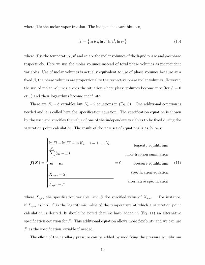
where β is the molar vapor fraction. The independent variables are,

X ={

lnKi, lnT, ln vl, ln vg

}(10)

where, T is the temperature, vl and vg are the molar volumes of the liquid phase and gas phase

respectively. Here we use the molar volumes instead of total phase volumes as independent

variables. Use of molar volumes is actually equivalent to use of phase volumes because at a

fixed β, the phase volumes are proportional to the respective phase molar volumes. However,

the use of molar volumes avoids the situation where phase volumes become zero (for β = 0

or 1) and their logarithms become indefinite.

There are Nc + 3 variables but Nc + 2 equations in (Eq. 8). One additional equation is

needed and it is called here the ‘specification equation’. The specification equation is chosen

by the user and specifies the value of one of the independent variables to be fixed during the

saturation point calculation. The result of the new set of equations is as follows:

f(X) =

lnF li − lnF g

i + lnKi, i = 1, ..., Nc

Nc∑i

(yi − xi)

P l − P g

Xspec − S

Pspec − P

= 0

fugacity equilibrium

mole fraction summation

pressure equilibrium

specification equation

alternative specification

(11)

where Xspec the specification variable, and S the specified value of Xspec. For instance,

if Xspec is lnT , S is the logarithmic value of the temperature at which a saturation point

calculation is desired. It should be noted that we have added in (Eq. 11) an alternative

specification equation for P . This additional equation allows more flexibility and we can use

P as the specification variable if needed.

The effect of the capillary pressure can be added by modifying the pressure equilibrium

10

equation in the system of equations in (Eq. 8). The resulting system of equations is the

following

f(X) =

lnF li − lnF g

i + lnKi, i = 1, ..., Nc

Nc∑i

(yi − xi)

P l − P g + Pc(x,y, vl, vg)

Xspec − S

= 0

fugacity equilibrium

mole fraction summation

pressure equilibrium

specification equation

(12)

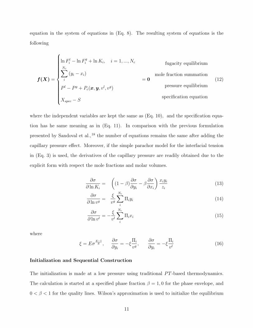
where the independent variables are kept the same as (Eq. 10), and the specification equa-

tion has he same meaning as in (Eq. 11). In comparison with the previous formulation

presented by Sandoval et al.,18 the number of equations remains the same after adding the

capillary pressure effect. Moreover, if the simple parachor model for the interfacial tension

in (Eq. 3) is used, the derivatives of the capillary pressure are readily obtained due to the

explicit form with respect the mole fractions and molar volumes.

∂σ

∂ lnKi

=

((1− β)

∂σ

∂yi− β ∂σ

∂xi

)xiyizi

(13)

∂σ

∂ ln vg=

ξ

vg

Nc∑i

Πiyi (14)

∂σ

∂ ln vl= − ξ

vl

Nc∑i

Πixi (15)

where

ξ = EσE−1E ,

∂σ

∂yi= −ξΠi

vg,

∂σ

∂yi= −ξΠi

vl(16)

Initialization and Sequential Construction

The initialization is made at a low pressure using traditional PT -based thermodynamics.

The calculation is started at a specified phase fraction β = 1, 0 for the phase envelope, and

0 < β < 1 for the quality lines. Wilson’s approximation is used to initialize the equilibrium

11

K-factors. It is then followed by 3-5 iterations using a partial Newton iteration method

neglecting the composition derivatives. The procedure is switched to a full Newton step

scheme using the set of independent variables X from (Eq. 10). When switching to the

V T -based variables, the volume of each phase is calculated from the EoS and one is selected

for the specification equation at the first iteration. The strategy presented in Michelsen34

can be employed to sequentially construct the phase envelope using sensitivity analysis

∂f

∂X

∂X

∂S+∂f

∂S= 0 (17)

where (∂X/∂S) is the vector of sensitivities. The most sensitive variable is used to specify

the next calculation point, and (∂X/∂S) is used to generate the initial estimates.

For the formulation in Eq. (11), the alternative specification can also be included in

the sensitivity analysis. In such case, the Jacobian (∂f/∂X) should be constructed for the

system with the alternative equation, and P is treated as an additional element in the vector

X. Moreover, to have a fair comparison with the other variables, the sensitivity of P should

be calculated in a ‘logarithmic’ manner as follows:

∂ logP

∂S≈ 1

1 + |P |∂P

∂S(18)

where the denominator has been modified to avoid indefinite values. Having the sensitivity

of P allows construction of a 3rd degree polynomial for interpolating/extrapolating to a

specified pressure value. A flowchart is provided in supporting information for visualization

of the described procedure.

The PT-flash using VT-based Thermodynamics

The solution of the PT -flash problem using PT -based thermodynamics corresponds to the

minimum of the system Gibbs energy. The problem is usually formulated as a minimization

12

subject to linear constraints on the mole numbers:

minng,nl

G(Tspec, Pspec,ng, nl), s.t. nz = ng + nl (19)

By setting the mole numbers in a certain phase (e.g. the liquid phase) as dependent

nli = nz

i − ngi , we convert the original problem to an unconstrained minimization with Nc

variables:

minng

G(Tspec, Pspec,ng) (20)

Michelsen4 showed that PT-flash can also be formulated as an unconstrained minimiza-

tion problem when V T -based thermodynamics is used. The state function to be minimized

with respect the mole numbers and the volume is

minng ,V l,V g

Q = minng,V l,V g

{A(Tspec,n

g, V l, V g) + V Pspec

}(21)

where A is the Helmholtz energy and V = V l + V g. The fact that the problem remains a

minimization problem for V T -based thermodynamics is particularly attractive since standard

minimization procedures using Newton steps can be employed

∆x = −H−1g (22)

where x is the set of independent variables x = {ng, V g, V l}. The gradient of the system

has the following form

g =

gi =∂Q

∂ngi

= ln f gi − ln f l

i , i = 1, ..., Nc

gNc+1 =∂Q

∂V g=

1

RT(−P g + Pspec)

gNc+2 =∂Q

∂V l=

1

RT

(−P l + Pspec

)(23)

where Q = Q/RT has been introduced for convenience. The Hessian matrix can be written

13

as follows

H =

Hij =∂gi∂ng

j

=∂ lnF g

i

∂ngj

− 1

βg+δijV g

+∂ lnF l

i

∂nlj

− 1

βl+δijV l, i, j = 1, ..., Nc

Hi,Nc+1 =∂gi∂V g

=∂ lnF g

i

∂V l

Hi,Nc+2 =∂gi∂V l

= −∂ lnF gi

∂V l

HNc+1,j =∂gNc+1

∂ngj

= − 1

RT

∂P g

∂ngj

=∂ lnF g

i

∂V g

HNc+2,j =∂gNc+2

∂ngj

=1

RT

∂P l

∂nli

= −∂ lnF li

∂V l

HNc+1,Nc+2 =∂gNc+1

∂V l= 0

HNc+2,Nc+1 =∂gNc+2

∂V g= 0

HNc+1,Nc+1 =∂gNc+1

∂V g= − 1

RT

∂P g

∂V g

HNc+2,Nc+2 =∂gNc+2

∂V l= − 1

RT

∂P l

∂V l

(24)

Notice that the elements of the Hessian matrix match those presented by Nichita.36 To

ensure a decrease of Q at each iteration, control on the step size and corrections to the Hessian

may be required to ensure positive definiteness.37,38 Initialization of the problem can be

performed either by stability analysis or by assuming 2-phases using Wilson’s approximation

for the equilibrium factors. In both cases, one to three updates of the phases fractions and

compositions based on PT -based Successive Substitution (i.e. assuming composition in-

dependent K-factors) are recommended before switching to the V T -based Newton step

procedure in (Eq. 22).

Inclusion of the Capillary Effect

Similar to the inclusion of the capillary pressure on the phase envelope calculations presented

in the previous section, capillary pressure can be introduced by modifying the gradient in

(Eq. 23). The capillary pressure term is included in gNc+1 as +Pc if the specification pressure

14

Pspec is the liquid pressure, or in gNc+2 as −Pc if Pspec is the gas pressure.

gNc+1 =1

RT(−P g + Pspec + Pc) or gNc+2 =

1

RT

(−P l + Pspec − Pc

)(25)

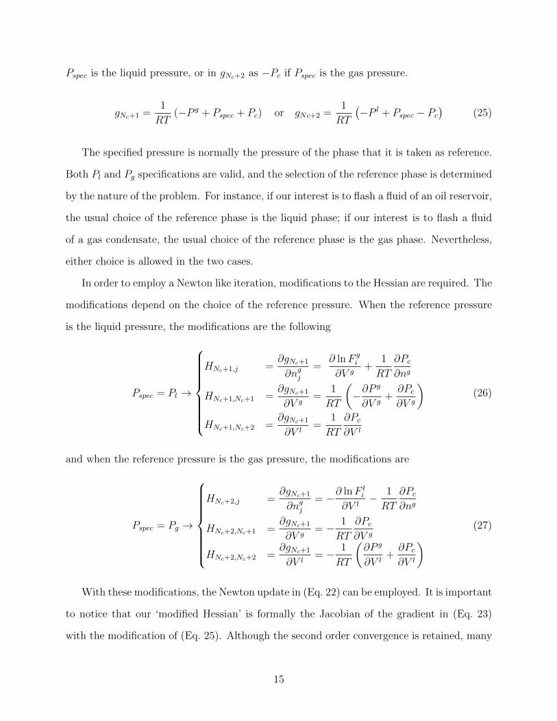
The specified pressure is normally the pressure of the phase that it is taken as reference.

Both Pl and Pg specifications are valid, and the selection of the reference phase is determined

by the nature of the problem. For instance, if our interest is to flash a fluid of an oil reservoir,

the usual choice of the reference phase is the liquid phase; if our interest is to flash a fluid

of a gas condensate, the usual choice of the reference phase is the gas phase. Nevertheless,

either choice is allowed in the two cases.

In order to employ a Newton like iteration, modifications to the Hessian are required. The

modifications depend on the choice of the reference pressure. When the reference pressure

is the liquid pressure, the modifications are the following

Pspec = Pl →

HNc+1,j =∂gNc+1

∂ngj

=∂ lnF g

i

∂V g+

1

RT

∂Pc

∂ng

HNc+1,Nc+1 =∂gNc+1

∂V g=

1

RT

(−∂P

g

∂V g+∂Pc

∂V g

)HNc+1,Nc+2 =

∂gNc+1

∂V l=

1

RT

∂Pc

∂V l

(26)

and when the reference pressure is the gas pressure, the modifications are

Pspec = Pg →

HNc+2,j =∂gNc+1

∂ngj

= −∂ lnF li

∂V l− 1

RT

∂Pc

∂ng

HNc+2,Nc+1 =∂gNc+1

∂V g= − 1

RT

∂Pc

∂V g

HNc+2,Nc+2 =∂gNc+1

∂V l= − 1

RT

(∂P g

∂V l+∂Pc

∂V l

) (27)

With these modifications, the Newton update in (Eq. 22) can be employed. It is important

to notice that our ‘modified Hessian’ is formally the Jacobian of the gradient in (Eq. 23)

with the modification of (Eq. 25). Although the second order convergence is retained, many

15

other properties are lost. Since the Jacobian is no longer symmetric, we cannot use a LDL

Cholesky factorization but use a slower LU factorization instead. Moreover, the procedure

is no longer a minimization and it is not possible to track the Q function in (Eq. 21). The

problem becomes an equation-solving problem and closer initial estimates are preferred. This

may require more successive substitution iterations at the initialization than the bulk flash.

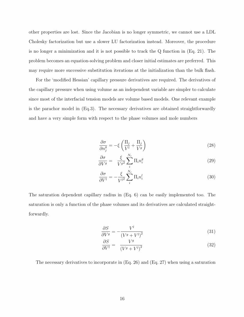
For the ‘modified Hessian’ capillary pressure derivatives are required. The derivatives of

the capillary pressure when using volume as an independent variable are simpler to calculate

since most of the interfacial tension models are volume based models. One relevant example

is the parachor model in (Eq.3). The necessary derivatives are obtained straightforwardly

and have a very simple form with respect to the phase volumes and mole numbers

∂σ

∂ngj

= −ξ(

Πj

V l+

Πj

V g

)(28)

∂σ

∂V g=

ξ

V g2

Nc∑i

Πingi (29)

∂σ

∂V l= − ξ

V l2

Nc∑i

Πinli (30)

The saturation dependent capillary radius in (Eq. 6) can be easily implemented too. The

saturation is only a function of the phase volumes and its derivatives are calculated straight-

forwardly.

∂S

∂V g= − V l

(V g + V l)2(31)

∂S

∂V l=

V g

(V g + V l)2(32)

The necessary derivatives to incorporate in (Eq. 26) and (Eq. 27) when using a saturation

16

dependent capillary radius are

∂Pc

∂ngj

=2 cos θ

rc(S)

∂σ

∂ngj

(33)

∂Pc

∂V g=

2 cos θ

rc(S)

∂σ

∂V g− 4σ cos θ

rc(S)2∂rc(S)

∂S

∂S

∂V g(34)

∂Pc

∂V l=

2 cos θ

rc(S)

∂σ

∂V l− 4σ cos θ

rc(S)2∂rc(S)

∂S

∂S

∂V l(35)

Notice that only an additional term in the derivatives of the capillary pressure with

respect to the volume is needed when a variable capillary radius is used instead of a fixed

one. This property is very attractive and easy to implement in more realistic simulations

scenarios where the pore size distribution of the porous media is important.

It is worthwhile mentioning that the presented PT -flash with capillary pressure can

be easily extended to the V T -flash specification problem. For the original formulation in

(Eq. 21), a minimization of the Helmholtz energy A instead of Q is required. The set

of independent variables is reduced to from Nc + 2 to Nc + 1 using the linear constraint

Vg = Vspec− Vl. As a result, the modified gradient of (Eq. 23) is also reduced to Nc + 1 with

gNc+1 = −Pg +Pl +Pc = 0. Solution of the V T -flash with capillary pressure using a dynamic

model has been recently presented in the literature.39

Initialization and Solution Procedure

Initialization is done using Wilson’s equilibrium K-factors followed by PT -based successive

substitution (SS) iterations. The PT-based SS requires solving the EoS but it is more ro-

bust than the VT-based SS. For the bulk case, if the first SS iteration yields in an increase

of the Gibbs energy or disappearance of a phase occurs, stability analysis is employed. If

unstable, a fixed number of SS iterations are taken before switching to Newton like steps.

When considering capillary pressure, checks on the Gibbs energy are no longer allowed since

it is not a minimization procedure. Therefore, SS iterations are taken until reaching an

intermediate tolerance ≈ 0.5 and the procedure is then switched to a Newton step using

17

the Hessian in (Eq. 24) with the modification of (Eq. 26). If a phase disappears during the

process, it is confirmed with the modified ‘stability analysis’ including capillary pressure.40

Good initial estimates are required for both the phase split calculation including capillary

pressure and the modified stability analysis before switching to second order methods since

it is no longer a minimization procedure. Therefore, the procedure is less robust than that

of the bulk case.

Results

Phase Envelope without Capillary Pressure

The V T -based phase envelope algorithm is applied to System I consisting of a ternary mix-

ture C1, C2 and C8 taken from Michelsen and Mollerup.35 The EoS-parameters are pre-

sented in the supporting information. The results for system I are presented in Figure 1.

Its construction is started from the dew point branch and continues to the bubble point

branch crossing the critical point. The phase envelope has intersecting phase boundaries at

the bubble point branch close to T = 200 K. This branch does not represent the real phase

boundary since there exists a narrow three-phase region at the vicinity of the intersection

which can be confirmed using stability analysis. For further details and discussion of the

three-phase region, please refer to Michelsen and Mollerup35 on chapter 12 and section 4.

Note that the tracing of the phase envelope continues to negative pressures and then comes

back without any problems because V T -based thermodynamics can naturally handle nega-

tive pressure values. This feature is not immediately obtained in a PT -based formulation.

Results with the same features have been obtained by Nichita with his density based phase

envelope algorithm. .41

18

100 200 300 400 500

0

100

200

300

T (K)

P(b

ar)

Critical Point

100 200 300 400 500

0

100

200

300

T (K)

Critical Point

Figure 1: Unusual hydrocarbon ternary system phase envelopes using V T -based formulation.[Left ] zfeed = {0.80, 0.15, 0.05}. [Right ] zfeed = {0.85, 0.05, 0.10}

.

Phase Envelope with Capillary Pressure

Three examples are presented in this section in order to test the algorithm proposed for

the phase envelope. No particular difficulties were observed. The obtained convergence is

quadratic as expected due to the Newton-based method approach implemented. For the

fluid description, the SRK-EoS was used for System II, III and IV, and the PR(78)-EoS42

for System V. The fluid description for each system is given as Supporting Information. The

Young-Laplace equation inside a tube in (Eq. 4) is selected to describe the capillary pressure

difference between the liquid and gas phase and the parachor model in (Eq. 3) to describe the

interfacial tension. The first example in Figure 2 represents a natural gas mixture made up

of seven components (System II). The results obtained match those of the PT -based phase

envelope calculations including capillary pressure presented by Sandoval et al.18 (Figure 2),

confirming the correctness of the results presented here. The algorithm handles different

capillary radii without any problem, obtaining quadratic convergence in each point along

the phase envelope. Shifts along the bubble point and the dew point are observed, except at

the critical point. A decrease in the bubble point branch and an inflated dew point branch

is observed in all the systems.

19

The results for System III and System IV are presented in Figure 3 and Figure 4 and

correspond to gas condensate systems described taken from Sherafati and Jessen,40 and

Whitson and Sunjerga43 respectively. The trace amounts of the heaviest components in sys-

tem III do not seem to affect the stability of the algorithm since the phase envelopes obtained

at different capillary radii are completely smooth. A sharp increase in the cricondentherm

compared to the other systems is observed. In general, gas condensates show larger shifts

in the dew point branch than oil systems. System III shows close to 25 K shift in the

cricondentherm at 5 nm and 50 K at 2 nm. System IV shows a more moderate change in

the cricondentherm compared to System III. Such difference can be attributed to the heavy

components in trace amounts of System III. Furthermore, System IV is a more conventional

gas condensate system, and the results are more representative for traditional gas condensate

systems. The calculations at rc = 2 are presented to show the stability of the code at high

capillary pressures. However, additional effects such as adsorption and confinement should

be taken into account if a more realistic description is required.

System V represents a black oil system from the Eagle Ford field taken from Orangi et

al.44 Figure 5 shows the results of the phase envelope at different capillary radii. This system

is characterized by having large interfacial tension values, yielding capillary pressures above

100 bar for a capillary radius of 2 nm. The system is a special case that represents a black

oil heavier than those typically reported for shale reservoirs. However, it exemplifies a fluid

in which capillary effects are of huge importance. If the reservoir temperature is between

300-400K, the saturation pressure shift for a 5 nm capillary radius is already higher than

20 bar. For the extreme case of 2 nm, the shift of the phase boundary is dramatic. The

modified saturation point is shifted to a very low-pressure value below 20 bar. The high

capillary pressure values corresponding to this capillary radius show the stability of the code

when high negative pressure values are found at low temperatures.

20

100 150 200 250 300−100

−50

0

50

100

T (K)

P(b

ar)

bulk

10 nm

5 nm

2 nm

10 nm18

Figure 2: Phase Envelope for a natural gas (system II) at different capillary radii rc includingresults from18 for comparison.

100 200 300 400 500−100

0

100

200

T (K)

P(b

ar)

bulk

10 nm

5 nm

2 nm

Figure 3: Phase Envelope for a gas condensate (system III) at different capillary radii rc

21

100 200 300 400 500 600−100

0

100

200

300

T (K)

P(b

ar)

bulk

10 nm

5 nm

2 nm

Figure 4: Phase Envelope for a gas condensate (system IV) at different capillary radii rc

100 200 300 400 500 600 700 800−300

−200

−100

0

100

200

T (K)

P(b

ar)

bulk

10 nm

5 nm

2 nm

Figure 5: Phase Envelope for Eagle-Ford black oil (system V) at different capillary radii rc

22

Figure 4: Phase Envelope for a gas condensate (system IV) at different capillary radii rc

100 200 300 400 500 600 700 800−300

−200

−100

0

100

200

T (K)

P(b

ar)

bulk

10 nm

5 nm

2 nm

Figure 5: Phase Envelope for Eagle-Ford black oil (system V) at different capillary radii rc

22

Flash

The flash code was tested for system II, III, IV, and V at different liquid pressure and

temperature specifications. The presented examples show the results at different capillary

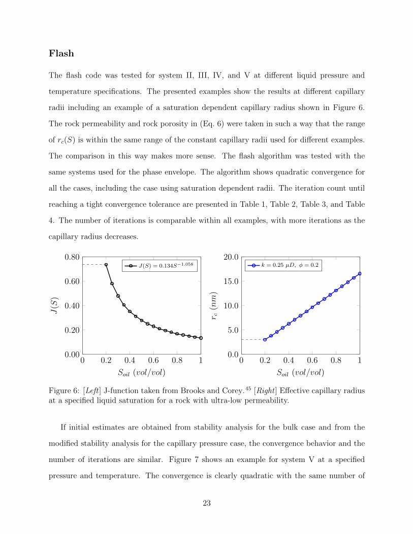
radii including an example of a saturation dependent capillary radius shown in Figure 6.

The rock permeability and rock porosity in (Eq. 6) were taken in such a way that the range

of rc(S) is within the same range of the constant capillary radii used for different examples.

The comparison in this way makes more sense. The flash algorithm was tested with the

same systems used for the phase envelope. The algorithm shows quadratic convergence for

all the cases, including the case using saturation dependent radii. The iteration count until

reaching a tight convergence tolerance are presented in Table 1, Table 2, Table 3, and Table

4. The number of iterations is comparable within all examples, with more iterations as the

capillary radius decreases.

0 0.2 0.4 0.6 0.8 10.00

0.20

0.40

0.60

0.80

Soil (vol/vol)

J(S

)

J(S) = 0.134S−1.058

0 0.2 0.4 0.6 0.8 10.0

5.0

10.0

15.0

20.0

Soil (vol/vol)

r c(nm

)

k = 0.25 µD, φ = 0.2

Figure 6: [Left ] J-function taken from Brooks and Corey.45 [Right ] Effective capillary radiusat a specified liquid saturation for a rock with ultra-low permeability.

If initial estimates are obtained from stability analysis for the bulk case and from the

modified stability analysis for the capillary pressure case, the convergence behavior and the

number of iterations are similar. Figure 7 shows an example for system V at a specified

pressure and temperature. The convergence is clearly quadratic with the same number of

23

iterations to reach the solution. Table 5 show the values of the vapor fraction at each iteration

and the values of the effective capillary radius for the saturation dependent case.

Table 1: Number of iterations at different PT -specifications and capillary radii for system II.Numbers inside parentheses are successive substitution steps and outside parentheses New-ton steps. SF = single phase, s = Initial estimate from stability analysis. (tolerance=10−10)

T (K) Pl (bar) bulk 10 (nm) 5 (nm) 2 (nm) rc(S)→ (nm)

150 1 2 (3) SF SF SF SF 16.58200 10 2 (3) 5 (3) 5 (4) 6 (4) 6 (3) 3.02200 50 6 (3) s 4 (3) 4 (3) 4 (3) 5 (3) 3.08225 10 2 (3) 6 (3) 6 (3) 6 (4) 5 (3) 3.02225 50 3 (3) s 3 (3) 3 (3) 4 (3) 5 (3) 3.02225 75 4 (3) s 5 (3) 4 (3) 3 (3) 3 (3) 3.02250 1 SF 5 (5) 4 (5) 6 (5) 5 (5) 3.02250 10 SF 4 (3) 5 (3) 5 (3) 5 (3) 3.02250 50 2 (3) s 3 (3) 3 (3) 5 (3) 4 (3) 3.02250 75 SF SF SF SF SF 3.02

Table 2: Number of iterations at different PT -specifications and capillary radii for system III.Numbers inside parentheses are successive substitution steps and outside parentheses New-ton steps. SF = single phase, s = Initial estimate from stability analysis. (tolerance=10−10)

T (K) Pl (bar) bulk 10 (nm) 5 (nm) 2 (nm) rc(S)→ (nm)

150 1 3 (3) SF SF SF SF 16.58200 10 3 (3) 5 (4) 5 (4) 9 (8) 6 (4) 3.27200 50 SF SF SF SF SF 16.58250 100 8 (3) s 7 (3) 6 (4) 6 (4) 8 (3) 5.40300 50 3 (3) 3 (3) 3 (4) 4 (4) 5 (3) 3.02300 120 5 (3) s 5 (3) 5 (3) 5 (3) 6 (3) 3.02350 10 2 (3) 4 (4) 5 (4) 5 (6) 6 (4) 3.02350 100 5 (3) 4 (3) 4 (3) 5 (3) 6 (4) 3.02380 10 3 (3) 5 (3) 6 (3) 7 (3) 8 (5) 3.02

24

Table 3: Number of iterations at different PT -specifications and capillary radii for system IV.Numbers inside parentheses are successive substitution steps and outside parentheses New-ton steps. SF = single phase, s = Initial estimate from stability analysis. (tolerance=10−10)

T (K) Pl (bar) bulk 10 (nm) 5 (nm) 2 (nm) rc(S)→ (nm)

150 1 1 (3) SF SF SF SF 16.58200 1 1 (3) 4 (3) 6 (3) SF 8 (3) 4.38200 50 SF SF SF SF SF 16.58300 10 3 (1) 4 (3) 4 (3) 8 (3) 6 (3) 3.02300 100 3 (3) 3 (3) 3 (3) 5 (3) 4 (3) 3.08300 150 7 (3) s 5 (3) 5 (3) 5 (3) 5 (3) 4.61400 10 1 (3) 4 (3) 4 (3) 7 (3) 5 (3) 3.02400 150 8 (3) s 4 (3) 4 (3) 5 (3) 4 (3) 3.02500 10 1 (3) 4 (3) 5 (3) 5 (3) 5 (3) 3.02500 150 7 (3) s 4 (3) 4 (3) 4 (4) 5 (3) 3.02

Table 4: Number of iterations at different PT -specifications and capillary radii for system V.Numbers inside parentheses are successive substitution steps and outside parentheses New-ton steps. SF = single phase, s = Initial estimate from stability analysis. (tolerance=10−10)

T (K) Pl (bar) bulk 10 (nm) 5 (nm) 2 (nm) rc(S)→ (nm)

200 10 2 (3) SF SF SF SF 16.58300 10 2 (3) 4 (3) 5 (3) SF 6 (3) 10.61400 10 2 (3) 3 (3) 4 (3) 5 (4) 6 (3) 7.62400 100 3 (3) 4 (3) SF SF 6 (3) 14.67500 10 2 (3) 4 (3) 5 (3) 6 (3) 6 (4) 5.22500 100 4 (3) 4 (3) 5 (3) SF 5 (3) 12.37600 10 2 (3) 5 (3) 6 (3) 4 (4) 7 (3) 3.02600 100 4 (3) 5 (3) 5 (3) 6 (6) 5 (3) 10.31700 50 4 (3) 5 (3) 7 (4) 6 (2) 5 (3) 3.02750 50 SF SF SF SF SF 3.02

Table 5: Values of β at each iteration and capillary pressure at the solution for the examplein Figure 7

iteration βbulk βrc=10 βrc=5 βrc=2 βrc(S) → rc(S) (nm)

1 0.3897440 0.3107606 0.2450603 0.0753131 0.2450603 8.61900222 0.4279117 0.3112307 0.2356720 0.0723429 0.2974333 7.72559033 0.4243932 0.3152221 0.2400675 0.0730090 0.2926242 7.81093604 0.4241739 0.3153344 0.2402755 0.0730130 0.2924600 7.81327625 0.4241734 0.3153346 0.2402761 0.0730130 0.2924599 7.81327816 0.4241734 0.3153346 0.2402761 — 0.2924599 7.8132781

Pc (bar) 0 23.42659 38.43796 62.14417 28.23014 —

25

0 2 4 6 8

−15

−10

−5

0

log‖g‖ ∞

bulk

10 nm

5 nm

2 nm

rc(S)

Iteration

25

Figure 7: Convergence plot of the gradient at different capillary radii using system V. Tspec =450 K, Pspec = 30 bar

Conclusions

We present in this paper how to solve two fundamental equilibrium calculation problems,

namely, phase envelope construction and flash calculation, in the presence of capillary pres-

sure by use of V T -based thermodynamics. V T -based thermodynamics has been previously

used in various phase equilibrium calculations for bulk phases. Compared with the classi-

cal PT -based thermodynamics, it avoids repeated solution of phase densities and can easily

handle negative pressure values. For calculations involving capillary pressures, it provides

the additional advantage that most capillary pressure expressions are functions of molar vol-

umes (e.g. in parachor models) and volume fractions (e.g. in the Leveret J function used to

account for pore size distribution) and it is much simpler to obtain the corresponding deriva-

tives required in the second-order methods. The explicit dependence of interfacial tension

and liquid saturation on phase volumes also makes the implementation easier.

Our phase envelope construction algorithm is a direct extension of Michelsen’s V T -based

phase envelope code. Compared with the PT -based algorithm, the V T -based code uses

26

the logarithm of phase molar volumes instead of the logarithm of pressure as independent

variables. This requires one more equation for equality of phase pressures in the phase

envelope construction for bulk phase. However, the introduction of capillary pressure does

not require an additional equation since a modification of the pressure equality equation is

sufficient. In comparison with PT -based phase envelope code with capillary pressure, the

number of equations is the same.

The V T -based flash involving capillary pressure has a similar form to the V T -based flash

for bulk phase (Michelsen, 1999). The only modification is to introduce capillary pressure

in the original pressure equality equations. This has unfortunately changed the problem

from a minimization problem to an equation solving one. The developed V T -based flash is

a second order method, and requires several rounds of successive substitution before it. The

successive substitution can be initialized by either the Wilson correlation or, more rigorously,

a modified stability analysis.

Three fluids (gas, gas condensate, and black oil) are used to test the developed phase

envelope and flash algorithms. A capillary radius down to 2 nm is used to test the algorithms

at extreme capillary pressure conditions. For the phase envelope code, the V T -based code

has given the same features in phase envelope shift as we obtained earlier with a PT -based

code. The V T -based code turns out to be particularly robust, having no problems with large

negative pressure values and showing second order convergence even at a capillary pressure

of several hundred bars. For the V T -based flash, the results show that more successive

substitution iterations are preferred when capillary pressure is considered, but the second

order iterations are nearly the same. Fast second order convergence can be obtained at

different capillary radii and also for the case considering pore size distribution.

Supporting Information

The Supporting Information is available free of charge on the ACS Publication website.

27

• System EoS Model Parameters

• Phase Envelope Construction Flowchart

Acknowledgments

We would like to acknowledge ConocoPhillips and ExxonMobil for their financial on the

COMPLEX project. We are also grateful to the Danish Hydrocarbon Research and Tech-

nology Centre for partly sponsoring this work.

References

(1) Heidemann, R. A.; Khalil, A. M. The Calculation of Critical Points. AIChE J. 1980,

26, 769–779.

(2) Nagarajan, N.; Cullick, A.; Griewank, A. New Strategy for Phase Equilibrium and Crit-

ical Point Calculations by Thermodynamic Energy Analysis. Part I. Stability Analysis

and Flash. Fluid Phase Equilib. 1991, 62, 191–210.

(3) Nagarajan, N. R.; Cullick, A. S.; Griewank, A. New Strategy for Phase Equilibrium

and Critical Point Calculations by Thermodynamic Energy Analysis. Part II. Critical

Point Calculations. Fluid Phase Equilib. 1991, 62, 211–223.

(4) Michelsen, M. L. State Function Based Flash Specifications. Fluid Phase Equilib. 1999,

158-160, 617–626.

(5) Nichita, D. V.; De-Hemptinne, J.-C.; Gomez, S. Isochoric Phase Stability Testing for

Hydrocarbon Mixtures. Pet. Sci. Technol. 2009, 27, 2177–2191.

(6) Mikyska, J.; Firoozabadi, A. A New Thermodynamic Function for Phase-Splitting at

Constant Temperature, Moles, and Volume. Am. Inst. Chem. Eng. J. 2011, 47, 1897–

1904.

28

(7) Jindrova, T.; Mikyska, J. Fast and Robust Algorithm for Calculation of Two-phase

Equilibria at Given Volume, Temperature, and Moles. Fluid Phase Equilib. 2013, 353,

101–114.

(8) Castier, M. Helmholtz Function-based Global Phase Stability Test and its Link to the

Isothermal-Isochoric Flash Problem. Fluid Phase Equilib. 2014, 379, 104–111.

(9) Jindrova, T.; Mikyska, J. General Algorithm for Multiphase Equilibria Calculation at

Given Volume, Temperature, and Moles. Fluid Phase Equilib. 2015, 393, 7–24.

(10) Nichita, D. V. Fast and Robust Phase Stability Testing at Isothermal-Isochoric Condi-

tions. Fluid Phase Equilib. 2017, 447, 107–124.

(11) Halldorsson, S.; Stenby, E. H. Isothermal Gravitational Segregation: Algorithms and

Specifications. Fluid Phase Equilib. 2000, 175, 175–183.

(12) Pereira, F. E.; Galindo, A.; Jackson, G.; Adjiman, C. S. On the impact of using vol-

ume as an independent variable for the solution of P-T fluid-phase equilibrium with

equations of state. Comput. Chem. Eng. 2014, 71, 67–76.

(13) Paterson, D.; Michelsen, M. L.; Stenby, E. H.; Yan, W. New Formulations for Isothermal

Multiphase Flash (SPE-182706-PA). SPE J. 2017, 20–22.

(14) White, W. B.; Johnson, S. M.; Dantzig, G. B. Chemical Equilibrium in Complex Mix-

tures. J. Chem. Phys. 1958, 28, 751–755.

(15) Paterson, D.; Michelsen, M.; Stenby, E.; Yan, W. Compositional Reservoir Simulation

Using (T, V) Variables-Based Flash Calculation. ECMOR XVI-16th European Confer-

ence on the Mathematics of Oil Recovery. 2018.

(16) Brusilovsky, A. I. Mathematical Simulation of Phase Behavior of Natural Multicom-

ponent Systems at High Pressures With an Equation of State. SPE 1992, February,

117–122.

29

(17) Shapiro, A. A.; Stenby, E. H. Thermodynamics of the Multicomponent Vapor-Liquid

Equilibrium under Capillary Pressure Difference. Elsevier Sci. B.V. 2001, 178, 17–32.

(18) Sandoval, D. R.; Yan, W.; Michelsen, M. L.; Stenby, E. H. The Phase Envelope of

Multicomponent Mixtures in the Presence of a Capillary Pressure Difference. Ind. Eng.

Chem. Res. 2016, acs.iecr.6b00972.

(19) Dong, X.; Liu, H.; Hou, J.; Wu, K.; Chen, Z. Phase Equilibria of Confined Fluids in

Nanopores of Tight and Shale Rocks Considering the Effect of Capillary Pressure and

Adsorption Film. Ind. Eng. Chem. Res. 2016, 55, 798–811.

(20) Fisher, L. R.; Israelachvili, J. N. Experimental Studies on the Applicability of the

Kelvin Equation to Highly Curved Concave Menisci. J. Colloid Interface Sci. 1981,

80, 528–541.

(21) Zhong, J.; Riordon, J.; Zandavi, S. H.; Xu, Y.; Persad, A. H.; Mostowfi, F.; Sinton, D.

Capillary Condensation in 8 nm Deep Channels. J. Phys. Chem. Lett. 2018, 9, 497–503.

(22) Yang, Q.; Jin, B.; Banerjee, D.; Nasrabadi, H. Direct Visualization and Molecular

Simulation of Dewpoint Pressure of a Confined Fluid in sub-10 nm Slit Pores. Fuel

2019, 235, 1216–1223.

(23) Thommes, M. Physical Adsorption Characterization of Nanoporous Materials. Chemie-

Ingenieur-Technik 2010, 82, 1059–1073.

(24) Shapiro, A.; Stenby, E. Kelvin Equation for a Non-Ideal Multicomponent Mixture.

Fluid Phase Equilib. 1997, 134, 87–101.

(25) Luo, S.; Lutkenhaus, J. L.; Nasrabadi, H. Use of Differential Scanning Calorimetry to

Study Phase Behavior of Hydrocarbon Mixtures in Nano-Scale Porous Media. J. Pet.

Sci. Eng. 2016, 1–8.

30

(26) Wang, L.; Parsa, E.; Gao, Y.; Ok, J. T. Experimental Study and Modeling of the Ef-

fect of Nanoconfinement on Hydrocarbon Phase Behavior in Unconventional Reservoirs

(SPE-169581-MS). SPE West. North Am. Rocky Mt. Jt. Meet. Denver, Colorado, USA,

2014.

(27) Al, M.; Nasrabadi, H.; Banerjee, D. Fluid Phase Equilibria Experimental Investigation

of Confinement Effect on Phase Behavior of Hexane, Heptane and Octane Using Lab-

on-a-Chip Technology. Fluid Phase Equilib. 2016, 423, 25–33.

(28) Travalloni, L.; Castier, M.; Tavares, F. W.; Sandler, S. I. Thermodynamic Modeling of

Confined Fluids Using an Extension of the Generalized van der Waals Theory. Chem.

Eng. Sci. 2010, 65, 3088–3099.

(29) Shapiro, A.; Stenby, E. Multicomponent Adsorption: Principles and Models. Adsorpt.

Theory, Model. Anal. 2002, 375–431.

(30) Rangarajan, B.; Lira, C. T.; Subramanian, R. Simplified local density model for ad-

sorption over large pressure ranges. AIChE J. 1995, 41, 838–845.

(31) Kunz, O.; Klimeck, R.; Wagner, W.; Jaeschke, M. Gerg Tm15 ; 2007.

(32) Nichita, D. V. Volume-based phase stability testing at pressure and temperature spec-

ifications. Fluid Phase Equilib. 2018, 458, 123–141.

(33) Sugden, S. A Relation Between Surface Tension, Density, and Chemical Composition.

J. Chem. Soc., Trans. 1924, 125, 1177–1189.

(34) Michelsen, M. Calculation of Phase Envelopes and Critical Points for Multicomponent

Mixtures. Fluid Phase Equilib. 1980, 4, 1–10.

(35) Michelsen, M.; Mollerup, J. Thermodynamic Models; Fundamentals & Computational

aspects ; 2007.

31

(36) Nichita, D. V. A volume-based approach to phase equilibrium calculations at pressure

and temperature specifications. Fluid Phase Equilib. 2018, 461, 70–83.

(37) Hebden, M. D. An Algorithm for Minimization Using Exact Second Derivatives ; 1973.

(38) McSweeney, T. Modified Cholesky Decomposition and Applications. Ph.D. thesis, The

University of Manchester, UK, 2017.

(39) Kou, J.; Sun, S. A Stable Algorithm for Calculating Phase Equilibria with Capillarity

at Specified Moles, Colume and Temperature Using a Dynamic Model. Fluid Phase

Equilib. 2018, 456, 7–24.

(40) Sherafati, M.; Jessen, K. Stability Analysis for Multicomponent Mixtures Including

Capillary Pressure. Fluid Phase Equilib. 2017, 433, 56–66.

(41) Nichita, D. V. Density-based phase envelope construction. Fluid Phase Equilib. 2018,

478, 100–113.

(42) Robinson, D. B.; Peng, D.-Y. The Characterization of the Heptanes and Heavier Frac-

tions for the GPA-Peng-Robinson Programs ; RR-28; Gas Processor Association, 1978.

(43) Whitson, C. H.; Sunjerga, S. SPE 155499 PVT in Liquid-Rich Shale Reservoirs. SPE

Annu. Tech. Conf. Exhib. San Antonio, Texas, 2012; pp 8–10.

(44) Orangi, A.; Nagarajan, N.; Honarpour, M. M.; Rosenzweig, J. Unconventional Shale

Oil and Gas-Condensate Reservoir Production, Impact of Rock, Fluid, and Hydraulic

Fractures (SPE 140536). Hydraul. Fract. Technol. Conf. Exhib. The Woodlands, Texas,

USA, 2011; pp 1–15.

(45) Brooks, R.; Corey, A. Hydraulic Properties of Porous Media; Colorado State University

Hydrology Papers; Colorado State University, 1964.

32

Graphical TOC Entry

100 120 140 160 180 200 220 240 2600

20

40

60

80

T (K)P

(bar

)

Steps

Start

Finish

Crit. point

For Table of Contents only

Graphical TOC Entry

100 120 140 160 180 200 220 240 260

0

20

40

60

80

T (K)

P(b

ar)

Start

Finish

Crit. point

For Table of Contents only

34

30

33