Voting Systems and Strategic Manipulation: an Experimental

Study ∗

Anna Bassi†

September 1, 2008

Abstract

This paper presents experiments analyzing the strategic behavior of voters under three voting

systems: plurality rule, approval voting, and the Borda count. Strategic behavior is significantly

different under each treatment (voting system). Plurality rule leads voters to play in a more so-

phisticated manner, but not necessarily insincerely, displaying the lowest levels of manipulation.

The opposite holds for the Borda count games, where players are the least sophisticated but

the most insincere. Approval voting shows intermediate levels of strategic behavior. In terms of

social efficiency, plurality rule unexpectedly performs better than both approval voting and the

Borda count. Yet, plurality rule is the weakest performer under Condorcet efficiency, whereas

approval voting and the Borda count perform remarkably well even with a small electorate.

∗Financial support from Andrew Schotter and the Center of Experimental and Social Sciences at NYU is gratefullyacknowledged. I would like to thank Guillaume Frechette, Rebecca Morton, and Andrew Schotter for their constantsupport and advice. I would also like to thank Steven Brams, Sean Gailmard, and Robert Veszteg for helpfulcomments. An earlier version of this paper was presented at the 2006 annual meetings of the MPSA and the APSA,at the 2006 Annual Summer Meeting of the Society for Political Methodology and at the 2006 annual meeting of theEconomic Science Association. Conference and discussion participants are thanked for useful comments. All errorsremain my own.

†NYU, Department of Politics, New York, NY, 10012. E-mail address: anna.bassi@nyu.edu.

1

1 Introduction

Voting is one of the chief foundations on which democracy and its political institutions are con-

structed and developed. Hence, understanding how citizens vote is key both to understanding

democratic processes and to constructing formal models of political institutions.

An issue in voters’ behavior that has long been of interest to political science scholars is whether

voters vote “sincerely” for their most preferred alternative or “strategically”, casting their vote for

a different alternative in order to induce a better outcome. Let us suppose a voter believes that her

most preferred candidate has little chance of competing for the lead in the election. Voting for such

a candidate may be “wasted.” The voter may decide to switch her vote to the expected leading

candidate she most prefers in order to make her vote “pivotal” in determining a better outcome

for herself. This is the trade-off a rational voter faces in an election. She must balance her relative

preference for the different candidates against the relative likelihood of influencing the outcome of

the election.

Gibbard (1973) proved that any preference aggregation method is vulnerable to strategic ma-

nipulation by voters. However it is not clear whether the strategic behavior of the voters leads to

outcomes that are less desirable than the more representative sincere outcomes. On the one hand,

a voting procedure should be thought of as a tool to aggregate the preferences of the society and

the more accurately that voting represents the true preferences, the better the elected political

institutions serve the society’s objectives. On the other hand, sophisticated voting outcomes may

be more efficient or superior to sincere outcomes, electing more often the Condorcet alternative.

As Palfrey (1989) claims, when voters behave in a strategic way and expect others to do the same,

they end up voting for one of the two leading candidates, making the Condorcet alternative more

likely to be elected.

One can think that some rules are more vulnerable than others and that the degree to which they

are empirically affected by strategic manipulation by voters in the elections provides an interesting

criterion for evaluating alternative voting rules.

This paper explores the extent that voters engage in such manipulation through the use of

laboratory experiments. The experiments are designed to evaluate the effect of different voting

systems and voter experience on the emergence of strategic behavior in committee elections and

how strategic manipulation affects the efficiency of the elections outcomes. Strategic behavior

is studied in a series of complete-information elections in which subjects know both their own

2

preferences and the preferences of each member of the committee. The committee is composed

of five subjects who are asked to vote to elect one of four candidates according to either plurality

voting, approval voting, or the Borda count. Abstention is not allowed, which is justified by the

small size of the electorate which makes each voter highly likely to be pivotal, and consequently

abstention a dominated strategy.

The experimental literature on voting in committees is wide and increasing. This line of research,

beginning with the landmark articles by Plott (1967), Fiorina and Plott (1978), McKelvey (1976,

1979), and Schofield (1983) explores the cooperative and non-cooperative theory predictions on

voting. The experimental works on multi-candidate elections focus on the fact that almost anything

can happen in equilibrium. The reason is that there are many Nash equilibrium voting strategies

(Palfrey 1989, Myerson and Weber, 1993). This work has been extended in a number of directions.

For example, Gerber, Morton, and Rietz (1998) analyze cumulative voting to see if it can improve

minority representation. Forsythe et al. (1996) explore the multi-candidate elections in a series of

experiments. They compare plurality rule, Borda Count (BC) and Approval Voting (AV), finding

that BC and AV produce better outcomes than plurality rule, in the sense that the Condorcet loser

won the election less frequently.

This paper departs from the existing literature, and in particular from the Forsythe et al. (1996)

paper with which it shares many of the same goals, by predicting unique equilibrium strategies and

by allowing for more than three candidates. The problem of multiplicity of Nash equilibrium

voting strategies is eliminated by adopting the iterated elimination of weakly dominated strategies

equilibrium refinement that allow for a unique sophisticated strategy. The number of alternatives

is increased to four to allow for a non-trivial analysis of voters’ strategic behavior under AV (with

three candidates every non-sincere vote is dominated by a sincere one, therefore there is no rational

reason for a voter to move from a sincere behavior to a sophisticated one).1

2 Strategic behavior

Strategy-proofness has received a great deal of attention in social choice theory, where it is frequently

discussed in the context of elections. The first impossibility result comes from Gibbard (1973) and1According to the definition of Brams and Fishburn (1978, 1983), when the number of candidates is less or equal

to three, the set of approval voting strategies may be partitioned in two subsets: “dominated” and “admissiblesincere” strategies. This implies that any Nash Equilibrium strategy is also admissible sincere. Extending thenumber of candidates to more than three generates a third subset of strategies that are neither admissible sincerenor dominated.

3

Satterthwaite (1975): given some basic conditions on the number of available alternatives and the

size of the electorate, they show that every election procedure which is non-dictatorial cannot be

strategy-proof.

Then, the question turns in designing a voting procedure that is the least manipulable. Ma-

nipulation occurs when a voter behaves strategically (insincerely) and he/she determines a change

in the outcome (i.e., being pivotal). Strategic behavior may be studied in two settings: on the one

hand strategic voting is decision-theoretic when individuals act optimally assuming that others in

the electorate will vote sincerely; on the other hand, a non-myopic voter might account for the

possibility of strategic voting behavior by others. To cope with this, a game-theoretic perspective

is required, such as that taken by Cox (1994) and Myerson and Weber (1993).

When an outcome is strategy proof - from individual deviations - it is a Nash equilibrium

in sincere strategies: the sincere strategy is the best reply to the other players’ action for every

player. As Gibbard pointed out, no voting system is able to produce a unique Nash equilibrium

with strategic voters using only sincere strategies. There may exist multiple Nash equilibria with

strategic voting. If the number of voters is greater or equal to three, any candidate may win in a

Nash equilibrium.

A way to deal with this problem of multiplicity of Nash equilibria is to look for equilibrium

refinements, such as ruling out weakly dominated voting strategies. Eliminating weakly dominated

strategies, as Besley and Coate (1997) argue, is a reasonable approach in voting games. The first

step of elimination simply amounts to no player voting for the worst-ranked alternative. But this

does not prevent voters from going one step further and recalculating which strategies are weakly

dominated for them given that other voters will not use the already deleted weakly dominated

strategies (to vote for their worst-ranked candidate).

Allowing players to be strategic and to anticipate that the other voters will not use the weakly

dominated strategies either ( iterative elimination of weakly dominated strategies), pins down a set

of possible outcomes in a voting game. This allows the computation of the sophisticated strategies

each voter should use to maximize his own utility for any of the different voting systems. When the

game is dominance-solvable, a unique sophisticated strategy for each player survives the elimination

process, leading to a unique equilibrium.2

As Rajan (1998) shows, any strategy chosen under the iterated weak dominance solution concept2The order of deletion of weakly dominated strategies doesn’t matter here because we assume strict preferences

and maximal simultaneous deletion of weakly dominated strategies as elimination algorithm (see Gale, 1953 and Luceand Raiffa, 1957).

4

can be justified by beliefs that are consistent with the equilibrium concepts, which requires the

assumption that players know each others’ beliefs. Common knowledge of rationality leads to

iterated weak dominance which results in perfect equilibria.

Moreno and Wooders (1996) prove that if a game is dominance solvable, then the unique NE is

also coalition-proof. The iterated elimination refinement produces an equilibrium that is not only

resistent to individual deviations but also to deviations by a coalition of players.

The literature about iterative elimination of weakly dominated strategies for predicting out-

comes in voting games dates back to the seminal contribution of Farquharson (1969). He calls a

voter “sophisticated” if, after considering all possible votes by others and seeing in which cases his

vote makes a difference, he/she eliminates strategies that are dominated and assumes all the other

voters do the same. This process tells the voter which strategies are best in all possible circum-

stances. He called this procedure “sophisticated voting” and defined a voting game “determinate”

if sophisticated voting led to a unique outcome.

The power of the dominance solvability as solution concept has been studied in several exper-

iments. The general finding (Nagel, 1995 and 1999) is that most of the subjects engage in up to

four steps of eliminations. However, the depth of reasoning and rate of learning seem to depend on

group size, sophistication of the players, and previous experience with the game.

The following will briefly characterize the three voting procedures analyzed in this paper. As-

sume that there are k ≥ 3 candidates and n voters; both k and n are finite. Each voter i has a

strict preference order over the set of candidates. When necessary, assume that the tie breaking

rule is to pick a candidate randomly among those that are receiving the most votes.

Definition 1 (Plurality Voting (PV)) Each voter casts a vote for one of the k candidates. The

winner is the candidate with the most votes.

As shown by De Sinopoli and Turrini (2002), in a four (or more) candidate PV game, the

iterated weak dominance equilibrium refinement eliminates all the Nash equilibria except for one,

leading to a unique NE strategy.

Definition 2 (Borda count (BC)) Each voter ranks k candidates giving k − s points to the sth

candidate. The winner is the candidate with the most points.

It has been proved that this system, above all others, is the one which forces voters to make

strategic decisions instead of encouraging sincere voting (Smith, 1999). Giving a high ranking to a

candidate who is the most viable challenger of a voter’s most preferred candidate hurts the chances

5

of the preferred candidate winning. For example, a voter might not want to risk giving points

to other candidates if his top choice is in a tight race. Then, given the number and strength of

candidates, a strategic voter may give a high rank to candidates unlikely to win and a low rank to

candidates who are in strong competition with a voter’s favorite candidate.

Definition 3 (Approval Voting (AV)) Each voter casts a vote for as many of the k candidates

as she wants. The winner is the candidate with the highest total number of votes.

The higher degree of freedom that this system allow to the voters (voters may choose how many

candidates to vote for) leads to non-uniqueness or non-definiteness of sincere strategy. Voting for

the most preferred alternative is undoubtedly sincere, but voting for both the most preferred and

the second most preferred alternative may be considered sincere as well. Since under AV a voter is

not limited to cast or to rank a defined number of alternatives, a sincere strategy is indeterminate.

Brams and Fishburn (1978, 1983) define admissible and sincere strategies under AV. They define

a strategy “admissible” if it is not dominated, always involves voting for a most-preferred candidate,

and never involves voting for a least preferred candidate. They define a strategy as “sincere” if,

for any given candidate that a voter casts a vote, the voter also casts a vote for all candidates the

voter ranks higher than that candidate.

From the definition of admissibility it follows that any weakly undominated strategy must belong

to either the set of “admissible sincere” or to the set of “admissible non-sincere” strategies. Notice

that when the number of alternatives is less than or equal to three, all the “admissible strategies”

are also “sincere,” meaning that the best reply strategies are always sincere as well.

Even if AV is subject to strategic manipulation, Brams and Fishburn (1978) argue that approval

voting is subject to a milder type of strategic manipulation: voters react to strategic considerations

by truncating their preference scale in a different way (setting their approval cutoff point higher or

lower in their scale), without any need to desert their first choice.

Yet, sincere voting typically implies non-strategic behavior. Even if the AV sophisticated strate-

gies belong to the set of the “admissible sincere” strategies, these strategies cannot be considered

as sincere, since they are the result of strategic considerations. As Niemi (1984) points out: “...The

fact the AV fails to yield a unique sincere strategy is of major significance: it means that, under

AV, to say voters use admissible sincere strategies is not equivalent to say that they make no strate-

gic calculation. The existence of multiple, equally sincere admissible strategies, suggests that AV

encourage strategic (albeit admissible) voting...”.

6

3 Experimental design

The experimental design focuses on the case in which information is complete and common to all

players. Information is one of the main determinants of strategic behavior: the incentive to vote

strategically increases with the precision and the type of information (private or common) available

to the voter. Not surprisingly, when voters are not perfectly or privately informed, strategic voting

exhibits negative rather than positive patterns (Feddersen & Pesendorfer, 1997). The intuition is

that the less or more private the information about preferences of other voters, the more a voter

is concerned about switching her vote in the wrong direction. This does not happen when voters

base their decisions on sources of information that are complete and common across voters. Each

voter can be assured that all others are observing the same information, and hence can coordinate

on an appropriate candidate that is believed to be the trailing candidates by all the voters.

The game-theoretic perspective adopted here may lead to the possibility of self-reinforcing

strategic voting. An initial perceived bias in favor of one particular candidate may lead to some

strategic voting away from less favored candidates. But this strategic switching increases the

incentive for others to vote strategically. This process continues until every subject plays a Nash

equilibrium “sophisticated strategy.”

In order to allow for learning, every subject participated in twenty, one-shot election rounds.

In order to eliminate repeated effects, every subject was randomly matched in a different group at

every round.

3.1 Recruitment and Organization

I conducted three sessions of computerized experiments using undergraduate students at New York

University during the Fall of 2005.3 The experiment was conducted at the Center of Experimental

and Social Sciences(C.E.S.S.) computer lab.

Each experimental session was played by students who enrolled in the NYU e-recruit subject

pool. Students had joined the subject pool voluntarily by completing a form online indicating

their interest in participating in experiments. When a student enrolled for participation in the

experiment, he or she was told only that she would participate in a “voting experiment” and that

“...the experiment will last about one hour. Subjects should earn between $10 and $25...”.

The experiment required each participant to cast one or more votes (abstention was not allowed)3The experiment was programmed and conducted with the software z-Tree, (Fischbacher 1999).

7

Table 1: Number of Observations.Session First 10 rounds Second 10 rounds # subjects # obs.

1 Plurality (CW) Plurality (Cycle) 10 2002 Plurality (Cycle) Plurality (CW) 10 2003 Approval Voting (CW) Approval Voting (Cycle) 10 2004 Approval Voting (Cycle) Approval Voting (CW) 10 2005 Borda Count (CW) Borda Count (Cycle) 10 2006 Borda Count (Cycle) Borda Count (CW) 10 200

Notes - The table reports for each voting systems and each sequence of treatments (in parenthe-ses), the total number of subjects who participated in the experiment and the total number ofobservations.

over the set of candidates. Every subject was asked to vote according to one of the three different

voting rules: PV, AV, and BC.

The experimental design employed a 3x2 design with three sessions and two treatment per

session. I ran the experiment on 60 subjects, 20 per session. The 20 subjects formed four groups,

each comprised of five subjects. To minimize any possible repeated-game influences on the outcomes

of the experiments, the participants were allowed to participate in only one session. Sessions

involved 20 rounds. Each subject was randomly grouped with different members in each round in

such a way that a subject was not in the same group of subjects more than once in each treatment.

Table 1 reports some summary statistics about the experiment.

Asking all the players in the same session to vote according to only one voting rule allows

them to learn how the voting system works during the experiment. This seems reasonable because

elections are usually run with a constant voting system over a long time interval. If a voting system

turns out to be relatively non-manipulable when voters know it well, this is a stronger argument

for its non-manipulability than if voters have only a brief experience with it.

Even if the group within which each subject was asked to play changes from round to round, the

preference profile of the group did not change for ten consecutive rounds. This facilitates learning

especially in small committees. Furthermore, if a voting system did turn out to be less manipulable

in small committees, the result is stronger than if it did so in large committees.

At the beginning of the 11th round, each subject was asked to play according to a different

preference ordering, which remained the same from that round until 20 rounds were completed.

This allowed two different treatments (associated with two different preference profiles) per session,

which provides a check for robustness of each voting system. In one treatment the preference profile

of the group allows for the existence of the Condorcet Winner; in the other there was a cycle of

8

Table 2: Payoffs Schedule.Period 1-10 A B C D Period 11-20 A B C D

Type 1 7 5 1 3 Type 1 3 7 1 5Type 2 7 5 1 3 Type 2 3 7 1 5Type 3 3 1 7 5 Type 3 7 1 5 3Type 4 3 1 7 5 Type 4 7 1 5 3Type 5 5 1 3 7 Type 5 3 5 7 1

Notes - The table reports the number of experimental points each subject would receive if anyof the four candidates won the election. In this session, subjects played the “Condorcet Winnertreatment” in the first ten periods and the “Cycle treatment” in the last ten periods.

preferences. The former treatment is referred to as the “Condorcet” (CW) treatment and the latter

as the “Cycle” treatment.

After all subjects had arrived, they were assigned to separate cubicles, each with a PC and

a desk. The cubicles were arranged so that the subjects could not see anyone except the ex-

perimenters, nor could they been seen by anyone except the experimenters. Subjects were given

instructions along with tables (Table 2) with the experimental points attached to every potential

winning candidate. The instructions specified that each earned experimental point would have been

converted into $, at a rate of 20 cents per point, at the end of the experiment.

Within each group, the payoff schedules were identical for every subject. Thus, each subject

knew his or her own payoffs, the payoffs of the other types in the group, and the number of subjects

of each type. However, subjects did not know the specific assignments of types nor the identities

of the other subjects with whom they were grouped.

The instructions were read aloud so that subjects had common knowledge of the voting rules.

After that, subjects were given an opportunity to ask questions. After the instructions, each

subject was randomly assigned the role of one of six types. Types stayed the same throughout the

experiment.

In each election each subject was asked to cast one or more ballots (according to the specific

voting system/treatment), and the candidate with the most votes was declared the winner. Subjects

were informed of the vote totals received by each candidate, how the different types cast their votes,

the winner of the election, and the payoffs each type received from the election (if a tie occurred

between two or more candidates, subjects received a payoff equal to the average value of the tied

winners).

9

3.2 Voting Equilibria

Preferences are induced in the experiment by a vector of payoffs attached to the alternatives

(ui1, ....u

ik), where ui

K is the payoff (in terms of experimental points) that voter i would receive

if candidate k won the election. The vectors of payoffs are shown in Table 2.

A social choice analysis of the preference profiles shows that candidate “D” is the Condorcet

alternative (the candidate who wins against every other candidate in pairwise comparisons) in the

“CW” treatment; that the Condorcet loser (the candidate who loses against every other candidate

in pairwise comparisons) is candidate “B” in the “CW” treatment and candidate “D” in the“Cycle”

treatment; and that candidate A is the social optimum (the candidate who maximizes the aggregate

payoff of the voting group) in both the treatments.

In order to make both the voting game and the analysis of the results simpler and more intuitive,

only symmetric voting strategies are considered (the strategies of the players depend only on their

preferences and not on payoff-irrelevant factors such as the particular identity of the voter). Three

comments are in order at this point.

First, I do not allow voters to abstain: abstention is always a weakly dominated strategy for

any voter (Brams, 1994) and so will be deleted at the first round of the iterated deletion process.

Second, since the strategy of voting for one’s worst alternative is always weakly dominated as

well as the strategy of not voting for one’s best alternative, this will be set as the first round of the

elimination process for each voting system.

Third, the voting games determined by the preference profiles in Table ?? are all dominance

solvable, but they have different characterizations: the number of strategies for each player increases

moving from PV (k) to AV (∑k

i=1(ki )) and to BC (k!). At the first step of elimination, the number of

undominated strategies under PV, AV, and BC are three, seven, and fourteen, respectively. Given

a larger set of strategies under BC, a greater number of steps of elimination of weakly dominated

strategies is required. PV and AV require three steps of eliminations in the Condorcet Winner

treatment and four steps in the Cycle treatment. BC requires six and eight steps respectively.

Under PV and BC, the sets of sincere and sophisticated strategies are singletons. Under AV, the

strategy that is the best reply after three steps of iterated elimination of weakly dominated strategies

belongs to the set of “admissible sincere” strategies. The “admissible non-sincere” strategy is always

weakly dominated in the iterative process of elimination. The Nash Equilibria of each election, after

n rounds of iterate elimination of weakly dominated strategies, are described in Table 3.

10

Table 3: Strategies and Equilibria.Voting Voter Sincere Sophisticated NESystem type Strategy Strategy Outcome

1 & 2 A APV 3 & 4 C C A

5 D ACW 1 & 2 A, AB, ABD AB

AV 3 & 4 C, CD, CDA CD Dtreatment 5 D, DA, DAC D

1 & 2 ABDC ABDCBC 3 & 4 CDAB DCBA D

5 DACB DACB1 & 2 B B

PV 3 & 4 A C C5 C C

Cycle 1 & 2 B, BD, BDA BDAAV 3 & 4 A, AC, ACD AC A

treatment 5 C, CB, CBA C1 & 2 BDAC BDAC

BC 3 & 4 ACDB CADB C5 CBAD CBAD

Notes - The table reports for each voting systems (first column) and each voter’s type (secondcolumn), the sincere and sophisticated (Nash Equilibrium) strategies. The last column tells theNash Equilibria. The upper panel refers to the ‘Condorcet winner treatment,’ the lower panel refersto the ‘Cycle’ treatment.

4 Experimental Results

In this section a summary of the election results and individual voter behavior is presented. First,

the election results are summarized for each of the three sessions and two treatments (section 4.1),

and the frequency with which particular candidates, like the Condorcet Winner wins the race is

compared. Second, the occurrence of the Duvergerian races is analyzed in the PV treatment (section

4.2). Third, the observed voters’ behavior is analyzed, and sophisticated voting (section 4.3) and

manipulation (section 4.4) is compared across the three voting systems and the two treatments.

Last, the Condorcet efficiency (section 4.5) and the social efficiency (section 4.6) of the election

results are discussed.

4.1 Summary of results

All voting systems may produce some undesirable paradoxes like electing the Condorcet loser or

failing to elect the Condorcet winner. Among different voting systems AV and BC are expected to

11

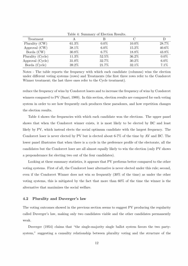
Table 4: Summary of Election Results.Treatment A B C D

Plurality (CW) 61.3% 0.0% 10.0% 28.7%Approval (CW) 38.1% 6.0% 15.2% 40.6%Borda (CW) 30.8% 6.7% 18.8% 43.8%

Plurality (Cycle) 11.3% 52.5% 36.2% 0.0%Approval (Cycle) 31.0% 32.7% 30.2% 6.0%Borda (Cycle) 39.2% 21.7% 32.1% 7.1%

Notes - The table reports the frequency with which each candidate (columns) wins the electionunder different voting systems (rows) and Treatments (the first three rows refer to the CondorcetWinner treatment; the last three ones refer to the Cycle treatment).

reduce the frequency of wins by Condorcet losers and to increase the frequency of wins by Condorcet

winners compared to PV (Saari, 1989). In this section, election results are compared for each voting

system in order to see how frequently each produces these paradoxes, and how repetition changes

the election results.

Table 4 shows the frequencies with which each candidate won the elections. The upper panel

shows that when the Condorcet winner exists, it is most likely to be elected by BC and least

likely by PV, which instead elects the social optimum candidate with the largest frequency. The

Condorcet loser is never elected by PV but is elected about 6-7% of the time by AV and BC. The

lower panel illustrates that when there is a cycle in the preference profile of the electorate, all the

candidates but the Condorcet loser are all almost equally likely to win the election (only PV shows

a preponderance for electing two out of the four candidates).

Looking at these summary statistics, it appears that PV performs better compared to the other

voting systems. First of all, the Condorcet loser alternative is never elected under this rule; second,

even if the Condorcet Winner does not win so frequently (30% of the time) as under the other

voting systems, this is mitigated by the fact that more than 60% of the time the winner is the

alternative that maximizes the social welfare.

4.2 Plurality and Duverger’s law

The voting outcomes showed in the previous section seems to suggest PV producing the regularity

called Duverger’s law, making only two candidates viable and the other candidates permanently

weak.

Duverger (1954) claims that “the single-majority single ballot system favors the two party-

system,” suggesting a causality relationship between plurality voting and the structure of the

12

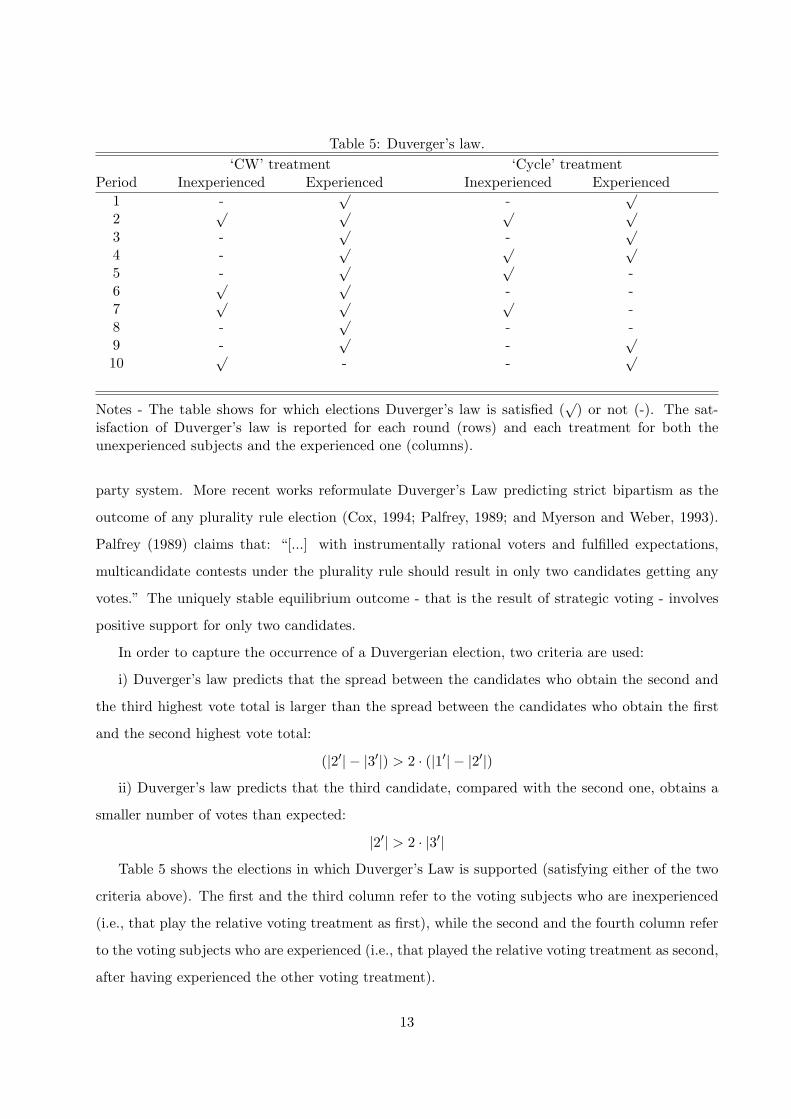
Table 5: Duverger’s law.‘CW’ treatment ‘Cycle’ treatment

Period Inexperienced Experienced Inexperienced Experienced1 -

√-

√2

√ √ √ √3 -

√-

√4 -

√ √ √5 -

√ √-

6√ √

- -7

√ √ √-

8 -√

- -9 -

√-

√10

√- -

√

Notes - The table shows for which elections Duverger’s law is satisfied (√

) or not (-). The sat-isfaction of Duverger’s law is reported for each round (rows) and each treatment for both theunexperienced subjects and the experienced one (columns).

party system. More recent works reformulate Duverger’s Law predicting strict bipartism as the

outcome of any plurality rule election (Cox, 1994; Palfrey, 1989; and Myerson and Weber, 1993).

Palfrey (1989) claims that: “[...] with instrumentally rational voters and fulfilled expectations,

multicandidate contests under the plurality rule should result in only two candidates getting any

votes.” The uniquely stable equilibrium outcome - that is the result of strategic voting - involves

positive support for only two candidates.

In order to capture the occurrence of a Duvergerian election, two criteria are used:

i) Duverger’s law predicts that the spread between the candidates who obtain the second and

the third highest vote total is larger than the spread between the candidates who obtain the first

and the second highest vote total:

(|2′| − |3′|) > 2 · (|1′| − |2′|)ii) Duverger’s law predicts that the third candidate, compared with the second one, obtains a

smaller number of votes than expected:

|2′| > 2 · |3′|Table 5 shows the elections in which Duverger’s Law is supported (satisfying either of the two

criteria above). The first and the third column refer to the voting subjects who are inexperienced

(i.e., that play the relative voting treatment as first), while the second and the fourth column refer

to the voting subjects who are experienced (i.e., that played the relative voting treatment as second,

after having experienced the other voting treatment).

13

The number of times that Duverger’s law is satisfied seems to be sensible to the preference

profile of the electorate, as data shows that turning from the “Condorcet Winner Treatment” to

the “Cycle treatment” reduces the Duverger’s law occurrence. Furthermore learning affects the

frequency of Duvergerian races, as Table 5 shows, when the subjects had experienced a former

treatment, the elections are more likely to be driven by two candidates.

4.3 Strategic behavior

As Farquharson (1969) suggests, if a voter doesn’t have a strategy which dominates every other

strategy, it is necessary for him/her to attempt to predict how the other voters are likely to vote

to make the best use of his/her vote. If a voter has complete information of the other voters’

strategies, this is sufficient to determine which strategies will not be chosen by the other voters

(being dominated), pinning down the number of possible contingencies that may be arise. But at

this point, the voter may reconsider his position on the basis of a smaller set of contingencies. This

method reaches conclusions by successively eliminating contingencies that will not happen.

However, the process of successively eliminating dominated strategies may require a substantial

amount of time, especially when the number of players increases. The voting games in our exper-

imental design are difficult to solve, and the experimental subjects are time constrained. Thus it

would not be surprising to find that subjects do not immediately play the sophisticated strategy, but

rather play different strategies over the course of the session, converging ultimately toward the so-

phisticated strategy (a QRE analysis which takes into consideration noise behavior in experimental

settings is discussed in detail in section 5). Furthermore, the preference profile of the electorate and

the voting procedure affects the players’ ability to converge or coordinate on particular equilibria.

The analysis of the voters’ behavior is summarized along the following hypotheses (the frequen-

cies with which each type played sophisticated, sincere, and dominated strategies are shown in

Table A1 and Table A2 in the Appendix).

Hypothesis 1: “Voting system” treatment effect. Sophisticated behavior is most likely

under PV and less likely under BC.

Sophisticated behavior increases as the number of iterated eliminations and the number of

strategies decreases. Since BC involves a number of eliminations greater than both PV and AV,

it will be likely to display the lowest level of sophisticated behavior. Furthermore, since the set of

strategies is smaller under PV than AV, then PV will be likely to display sophisticated behavior

14

Table 6: Sophisticated behavior.‘CW treatment’ ‘Cycle treatment’

PV AV BC PV AV BCPooled 0.69 0.45 0.27 0.71 0.40 0.35

Inexperienced 0.71 0.47 0.21 0.61 0.38 0.35Experienced 0.66 0.42 0.32 0.81 0.42 0.35

Notes - The table reports the frequency with which subjects played the sophisticated strategy. Foreach voting system and each treatment, three statistics are given: the first row for each type reportsthe frequency for the pooled subjects, the second row for the non experienced subjects, and thethird row for the experienced subjects (who experienced a early treatment).

more often than AV.

Hypothesis 2: “Preference Profile” Treatment effect. Sophisticated behavior is more

likely in the CW treatment than in the Cycle treatment.

Since the “Cycle treatment” implies a greater number of eliminations than the “CW treatment,”

it will be less likely to display sophisticated behavior.

Hypothesis 3: Learning. Sophisticated behavior increases as the number of voting games

experienced by the subjects increases.

Hypothesis 1.

Table 6 summarizes the frequency with which the experimental subjects chose the sophisticated

strategy in each preference profile and voting system treatment. From this first descriptive analysis,

it seems clear that there is a distinction between the ability to behave sophisticatedly under the

three voting systems. Plurality appears to be the system that induce the players to play the

sophisticated strategy the most (70%), while the Borda Count appears to be the one that is less

likely to lead players to behave in a sophisticated manner. Players under AV play the sophisticated

strategy 40%-45% of the time, which is a fairly standard result in a game involving three steps of

iterative eliminations.

I test the null hypothesis that the sophisticated behavior for the three voting system treatments

comes from populations with the same median using a Wilcoxon non-parametric rank sum test.

Comparing pairwise all three voting treatments (pooling data across CW and Cycle treatments),

the equality of the median is rejected at a 5% significance level (P-value=5.62e-007 for PV vs

AV, P-value=5.36e-013 for PV vs BC, P-value=0.0374 for AV vs BC). When comparing the three

15

voting systems according to the preference profile treatments, the results do not change but for the

comparison between AV and BC, for which the equality cannot be rejected at a 5% significance

level (P-value=0.88).

In addition, I also used a Kolmogorov-Smirnov test to examine whether the distribution of

the observed payoffs was the same across the two treatments. Consistent with the results of

the Wilcoxon test, the equality of distributions is rejected at a 5% significance level for all the

comparing voting systems (P-value=9.36e-005 for PV vs AV, P-value=6.02e-011 for PV vs BC,

P-value=0.0446 for AV vs BC). Even here, comparing the three voting systems according to the

preference treatments, the results do not change but for the comparison between AV and BC, for

which the equality cannot be rejected at a 5% significance level (P-value=0.63).

Both the descriptive and the statistical analyses suggest that sophisticated behavior under

different voting systems is significantly different.

Hypothesis 2.

From Table 6 it is not clear if the preference profile has a significative effect on the sophisticated

behavior. Wilcoxon and Kolmogorov-Smirnov tests are used again to test the effect of the preference

profile treatment.

According to Wilcoxon non-parametric rank sum test, the equality of the median under the “CW

treatment” and the “Cycle treatment” cannot be rejected at a 5% significance level for PV and AV,

while it is rejected for BC (P-value=0.8522 for PV, P-value=0.3881 for AV, and P-value=0.0592

for BC).

A Kolmogorov-Smirnov test confirms the above tests for PV and AV but not for BC: the equality

of distributions cannot be rejected at a 5% significance level for all the comparing voting systems

(P-value=0.6289 for PV, P-value=0.9808 for AV, P-value=0.6289 for BC). When the distribution of

frequency of sophisticated choices is compared, instead of the median, the equality of distributions

cannot be rejected.

The sophisticated behavior of the players, controlling for the voting system treatment, is not

affected by the preference profiles of the voting group. As shown by the data, the fact that the

preference profile allows for the existence of a Condorcet alternative does not lead to the voters

choosing more sophisticated strategies.

16

Hypothesis 3.

The experimental results do not show any general learning effect in the later rounds. However,

as Table A1 and A2 report, the data show a significant experience effect: subjects who experienced

an early treatment played less randomly than subjects who did not (the standard deviation for all

strategies is significantly lower).

4.4 Manipulation

In order for a scheme to be manipulable, there must be at least one voter whose insincere voting

can cause a change in the set of the winning alternatives.

The most used indices of manipulability like the “tainted”, the “F1”, and the “expected” index

(see Smith, 1999) measure the susceptibility of a voting rule to strategic voting by computing

the benefit a voter would enjoy by misrepresenting her true preference ordering, requiring the

definiteness of the voters’ sincere strategy. Since AV sincere voting is not definite, an alternative

index of manipulability must be used to compare the manipulability of the three voting systems.

Manipulation occurs when a voter votes insincerely and he/she is pivotal. Then, in order to

have a measure of the manipulation which occurred in the experiment, we compute the number of

times the experimental subjects cast an insincere vote that induced a change in the outcome. As

discussed in section 2, under PV and BC, there is a unique sincere strategy, while under AV, all

the strategies in the set of “admissible sincere” set are equally potentially sincere.

We adopt here three definitions of sincerity under AV:

1. Admissible sincerity: every strategy in the “admissible sincere” set is sincere (Brams and

Fishburn, 1978, 1983).

2. Non-sophisticated sincerity: every strategy in the “admissible sincere” set but the sophisticated

strategy is sincere. Since voters can play strategically by deviating to the “admissible sincere”

sophisticated strategy; only non-sophisticated admissible sincere strategies are considered as

sincere.

3. Pure sincerity: an AV strategy is sincere if a vote is casted for all the candidates whose utility

exceeds the expected utility of the election (Merrill, 1988). Since voters know with certainty

the preferences of every other voter, the expected utility is calculated by assuming that the

other voters play the sophisticated strategy.

17

si,t is defined as the sincere vote and ni,t the insincere vote cast by voter i in round t, where

N is the number of voters and T is the number of rounds. The manipulability index of a voting

system is defined as the frequency with which voters cast pivotal (with probability pi,t) insincere

votes.

M =T∑t

N∑

i

ni,tpi,t

NT(1)

Table 7 reports the score of the different voting systems. BC shows a higher manipulability with

respect to PV in every statistic. Furthermore, as Table A1 and A2 show, most of the insincere votes

are dominated strategies, meaning that voters manipulate the voting outcome in a non-rational way

(choosing weakly dominated strategies).

Table 7 shows how different definitions of AV sincere strategy are critical in determining the

level of manipulation to which AV is vulnerable.

According to the definition of Brams and Fishburn (1978, 1983), with four alternatives, there

are three admissible sincere strategies. Since proposition 4 shows that all the strategies that do not

belong to the “admissible sincere” set are dominated, according to this definition, manipulation

happens only when voters play dominated strategies. Data show that this type of manipulation

occurs 15%-20% of the time.

Yet, this definition doesn’t take into account the possibility of manipulating the outcome devi-

ating to “admissible sincere” strategies, which is shown in section 4.3 to occur 40%-45% of the time.

If voters manipulate the outcome by deviating to “admissible sincere” strategies (Niemi, 1984), then

this strategy cannot be considered as sincere. Data show that this type of manipulation occurs

between 50% and 60% of the times.

According to the definition of pure sincerity given by Merrill (1984), data shows that manipu-

lation occurs between 60% and 80% of the times.

As one turns from the first definition to the second, and then to the third, the set of sincere

strategies becomes smaller and smaller (with four alternatives there are three, two and one sincere

strategies respectively). Not surprisingly, the level of manipulability increases monotonically as the

definition of AV sincere strategies becomes more restrictive (i.e., as the sincere strategy set shrinks).

18

Table 7: Individual manipulation.PV BC AV (1) AV (2) AV (3)

Pooled 0.25 0.63 0.13 0.58 0.60‘CW treatment’ Inexperienced 0.27 0.68 0.10 0.57 0.65

Experienced 0.24 0.58 0.16 0.58 0.55Pooled 0.30 0.48 0.18 0.58 0.81

‘Cycle treatment’ Inexperienced 0.25 0.46 0.29 0.67 0.76Experienced 0.35 0.56 0.06 0.48 0.85

Notes - the table reports the manipulability score for the three voting systems under the twotreatments (upper and lower panel). The three AV scores refer to different definition of sincerity.For each voting system three statistics are given: the first row for each voting system reports thescore for the pooled subjects, the second row for the non-experienced subjects, and the third rowfor the experienced subjects (who experienced a early treatment).

4.5 Condorcet-Efficiency

Numerous criteria have been suggested to help select which voting systems, among various systems

for choosing winners from profiles, best reflect the cumulative will of the electorate. One of the most

common of these is the Condorcet criterion. A candidate is the Condorcet winner if she defeats

each candidate in pairwise majority elections. It is well known that a Condorcet winner need not

exist. However, many feel that a reasonable voting system should elect the Condorcet alternative

whenever such a candidate exists; this is called “Condorcet efficiency”.

For each voting system, Condorcet Efficiency is measured as the percentage of a given class of

elections for which the Condorcet candidate is chosen. Table 8 reports the Condorcet efficiency

score of each voting system. Consistent with the findings of other authors, even in small electorates,

PV is the weakest performer, whereas AV and BC perform quite well (with the latter being the

most likely to produce efficient outcomes consistent with Merrill’s work (1984)).

However, the last three rounds of each voting treatment highlight that under PV voters learn

how to manipulate the outcome in a way to elect the Condorcet alternative, while the frequency

with which it is elected under the other voting systems decreases in the last rounds.

None of the voting systems considered in the experimental analysis guarantees the selection

of the Condorcet alternative, but we can see how the sophisticated outcomes are superior to the

sincere outcomes. Recall what the sincere and the sophisticated outcomes would be for each voting

system. The theoretical Condorcet efficiency if every player behaved sincerely would be 0% for PV,

23% for AV, and 50% for BC. Instead, the theoretical Condorcet efficiency if every player behaved

sophisticatedly would be 0% for PV and 100% for AV and BC, since the NE candidate for the

19

Table 8: Condorcet Efficiency.Period Plurality Approval Borda

1 12.5% 33% 50%2 25% 50% 62.5%3 12.5% 37.5% 37.5%4 37.5% 25% 83%5 37.5% 37.5% 58%6 25% 65% 25%7 25% 54% 0%8 25% 54% 33%9 50% 25% 62.5%10 37.5% 25% 25%

Average 29% 41% 44%Last 3 37.5% 34.6% 40.16%

Per. AvSincere Outcome 0% 23% 50%

Sophisticated Outcome 0% 100% 100%

Notes - The Condorcet Efficiency is defined as the percentage of a given class of elections for whichthe Condorcet candidate is chosen. The Condorcet efficiency is reported for each round (rows) andeach voting system (columns). After the tenth period row, the overall average and the average ofthe last three periods is reported. The last two rows indicate what the Condorcet Efficiency wouldbe for the sincere and the sophisticated outcomes (breaking the ties with a fair coin and assumingthat under approval voting voters randomizes between sincere strategies).

latter ones coincides with the Condorcet winner.

4.6 Social Welfare Efficiency

The second measure of efficiency considers the value of each candidate for the entire electorate as

compared with other candidates. As distinct from the notion of Condorcet efficiency, the intensity

of the electorate’s preferences are weighted. Since the intensities of the preferences is usually not

revealed and difficult to discover by a researcher, this measure of efficiency is used less frequently

than the first one. An experimental analysis allows an analysis on intensity of preferences, since

subjects’ preferences are functions of the payoffs they receive at the end of the experimental session.

Following Harsanyi (1977), the “social optimum” is the candidate who maximizes the sum of

all voters’ utilities. Therefore “social efficiency” of a voting system is the normalized ratio between

the expected social utilities of the candidate selected by the system and the candidate maximizing

social utility.

Table 9 reports the performance of each voting system. Unexpectedly the PV System performs

20

Table 9: Social Efficiency.Plurality Approval Borda

Period CW Cycle CW Cycle CW Cycle1 0.93 0.90 0.92 0.88 0.96 0.962 0.95 0.91 0.96 0.91 0.89 0.913 0.96 0.87 0.91 0.87 0.94 0.834 0.94 0.88 0.95 0.87 0.87 0.905 0.95 0.87 0.81 0.92 0.93 0.836 0.95 0.89 0.89 0.88 0.80 0.877 0.98 0.88 0.87 0.93 0.82 0.918 0.95 0.92 0.89 0.95 0.79 1.009 0.96 0.89 0.95 0.89 0.92 0.8610 0.94 0.89 0.92 0.88 0.95 0.93

Average 0.95 0.89 0.91 0.90 0.89 0.90Sincere Outcome 0.88 0.96 0.96 0.87 0.96 0.91

Sophisticated Outcome 1 0.83 0.92 1 0.92 0.83

Notes - The Social Efficiency of a voting system is calculated as the ratio between the expectedsocial utilities of the elected candidate and the social optimum. The social efficiency is reportedfor each round (rows) and each voting system in both the CW treatment and Cycle treatment(columns). After the tenth period row, the overall average and the average of the last three periodsis reported. The last two rows indicated what the social efficiency would be for the sincere and thesophisticated outcomes (breaking the ties with a fair coin and assuming that under approval votingvoters randomize between sincere strategies).

significantly better than both AV and BC in the Condorcet winner treatment and approximately the

same as the other two voting systems in the cycle treatment. The explanation is simple: in the first

treatment, the PV system’s Nash Equilibrium, that is the actual outcome in 61% of experimental

elections, is the social optimum candidate. Besides this case, the measure of social efficiency is

approximately the same across voting systems and treatments.

Note that the social optimum candidate is not always the Condorcet candidate. That is, the

Condorcet criterion and the criterion of maximizing social utility may be different. However, the

Condorcet candidate yields a high level of social efficiency, even if not the highest one.

Recalling again the sincere and the sophisticated outcomes of each voting system, we can now

analyze if the sophisticated outcomes are superior to the sincere outcomes in terms of social welfare.

Under BC, sincerity always has a positive effect on the social welfare of the society, but under PV

and AV this effect is not clear, depending on the preference profile of the voting group.

As Table 9 shows, sophisticated behavior may not necessarily lead to more socially efficient

outcomes: when players act on the basis of individual self-interest alone, their behavior could lead

21

to the degradation of the social welfare of the electorate.

5 Quantal Response Equilibrium analysis

Iterated elimination of dominated strategies relies extensively on the assumption of perfect ra-

tionality. However, choice behavior in laboratory is shown to be noisy, revealing mistakes and

inconsistencies over time. In order to evaluate the iterated elimination procedure using data from

laboratory experiments, it is convenient to model a type of noisy behavior that includes the rational-

choice Nash predictions as a limit case.

One way to relax the assumption of noise-free, perfectly rational behavior is to specify a utility

function with a stochastic component. Probabilistic choice models (e.g., logit, probit) have long

been used to incorporate stochastic elements into the analysis of individual decisions, and the quan-

tal response equilibrium (McKelvey and Palfrey, 1995) is the analogous way to model games with

noisy players. The quantal response equilibrium (QRE) is a statistical version of Nash equilibrium,

where every strategy is played with positive probability. Players’ beliefs about other players’ ac-

tions determines players’ expected payoffs from different strategies, which in turn, generates choice

probabilities according to some quantal response function.

An identical and independently distributed stochastic term λ, accounting for the noise in the

best replies, is added to the expected payoff of each strategy. In the absence of noise (λ=0), the

QRE equilibrium reduces to a Nash equilibrium. Hence, the equilibria described in section 3.2

are limit cases of the quantal response equilibria described here. In order to provide parametric

estimates, a logit specification of the QRE is analyzed, where the quantal response functions are

logit curves, and λ is the response parameter.

The Quantal response functions for the PV and AV games, which describe the voting probability

as “noisy best responses” to the expected payoff of different strategies, are presented in figure 1

and 2 respectively.

Figure 1 presents the relationship between the probability of playing different strategies under

PV and the equilibrium values of λ along with the estimated values for both the Condorcet winner

treatment and the Cycle treatment. The curves in the plots show the equilibrium probability

of playing each of the three strategies associated with given values of λ. For λ = 0, the QRE

predicted probability is equal to 0.33. As λ increases, the equilibrium probability of playing the

equilibrium strategy (section 3.2) approaches one, while the equilibrium probability of playing the

22

0 5 100

0.2

0.4

0.6

0.8

1

λ

Typ

e 1&

2

0 5 100

0.2

0.4

0.6

0.8

1

λT

ype

3&4

0 5 100

0.2

0.4

0.6

0.8

1

λ

Typ

e 5

0 5 100

0.2

0.4

0.6

0.8

1

λ

Typ

e 1&

2

0 5 100

0.2

0.4

0.6

0.8

1

λ

Typ

e 3&

4

0 5 100

0.2

0.4

0.6

0.8

1

λ

Typ

e 5

CONDORCET WINNER TREATMENT

{A}

{D}

{B}

{C}

{D} {A}

{D}

{A} {C}

{B}

{D}

{A}

{C} {A}

{D}

{C} {B} {A}

CYCLE TREATMENT

Figure 1: Quantal Response Equilibrium functions for PV Games

other strategies approach zero. The vertical lines denote unconstrained estimated value of λ, and

the small circles denote the observed frequency with which each strategy is played.

Figure 2 presents the quantal response functions for AV games. The curves in the plots show

the equilibrium probability of playing each of the four strategies (three “admissible” and one “not

admissible”) associated with given values of λ. For λ = 0, the QRE predicted probability is equal

to 0.25. As λ increases, the equilibrium probability to play the equilibria strategy (section 3.2)

approaches one. The vertical lines denote the unconstrained estimated value of λ, and the small

circles denote the observed frequency with which each strategy is played.

Table 10 reports the estimates of the QRE for the plurality and approval voting games. The

table reports two estimated values of the error term λCW and λCycle for the two voting treatments.

The hypothesis that a unique parameter explain the behavior of the subjects for each voting systems

has been tested (H0 : λCW − λCycle = 0). The estimated values for λ in the two voting treatments

are λPV = 1.84 and λAV = 1.28 and the value of the Log Likelihood function is −219.96 and

−404.76 respectively. For both PV and AV, using a likelihood ratio test, the difference between

23

0 5 100

0.2

0.4

0.6

0.8

1

λ

Typ

e 1&

2

0 5 100

0.2

0.4

0.6

0.8

1

λT

ype

3&4

0 5 100

0.2

0.4

0.6

0.8

1

λ

Typ

e 5

0 5 100

0.2

0.4

0.6

0.8

1

λ

Typ

e 1&

2

0 5 100

0.2

0.4

0.6

0.8

1

λ

Typ

e 3&

4

0 5 100

0.2

0.4

0.6

0.8

1

λ

Typ

e 5

{A} {AB} {ABD, AD}

{C}

{CD}

{CDA} {CA}

{D}

{DA} {DAC}

{DC}

CONDORCET WINNER TREATMENT

CYCLE TREATMENT

{B} {BD}

{BDA}

{BA}

{A}

{AC}

{ACD}

{AD}

{C}

{CB}

{CBA} {CA}

Figure 2: Quantal Response Equilibrium functions for AV Games

λCW and λCycle is significant (the χ2 equals 12.58 and 22.94 respectively), suggesting that a unique

parameter cannot explain the behavior of the subjects in different strategic environments.

As shown by table 10, the QRE estimated probability fits the data better than the Nash

predictions, especially under PV which shows a larger log likelihood value with respect to AV. The

likelihood ratio test suggests that a same estimation for the “noise” does not explain the behavior

under the two treatments: in the cycle treatment, players’ best responses are much more noisy

than under the Condorcet winner treatment.

By combining behavior across voting systems, one can analyze whether the effect of different

preference aggregation methods on overall voting behavior is different. The estimations of lambda,

constrained to be equal across voting treatments, is λCW = 1.70 (LogL=318.31) and λCycle = 1.81

(LogL=313.73) for the Condorcet winner and cycle treatments respectively. For both treatments,

using a likelihood ratio test, the difference between λCW and λCycle is significant (the χ2 equals

26.00 and 24.15 respectively), suggesting that a unique parameter cannot explain the behavior of

the subjects under different voting systems.

24

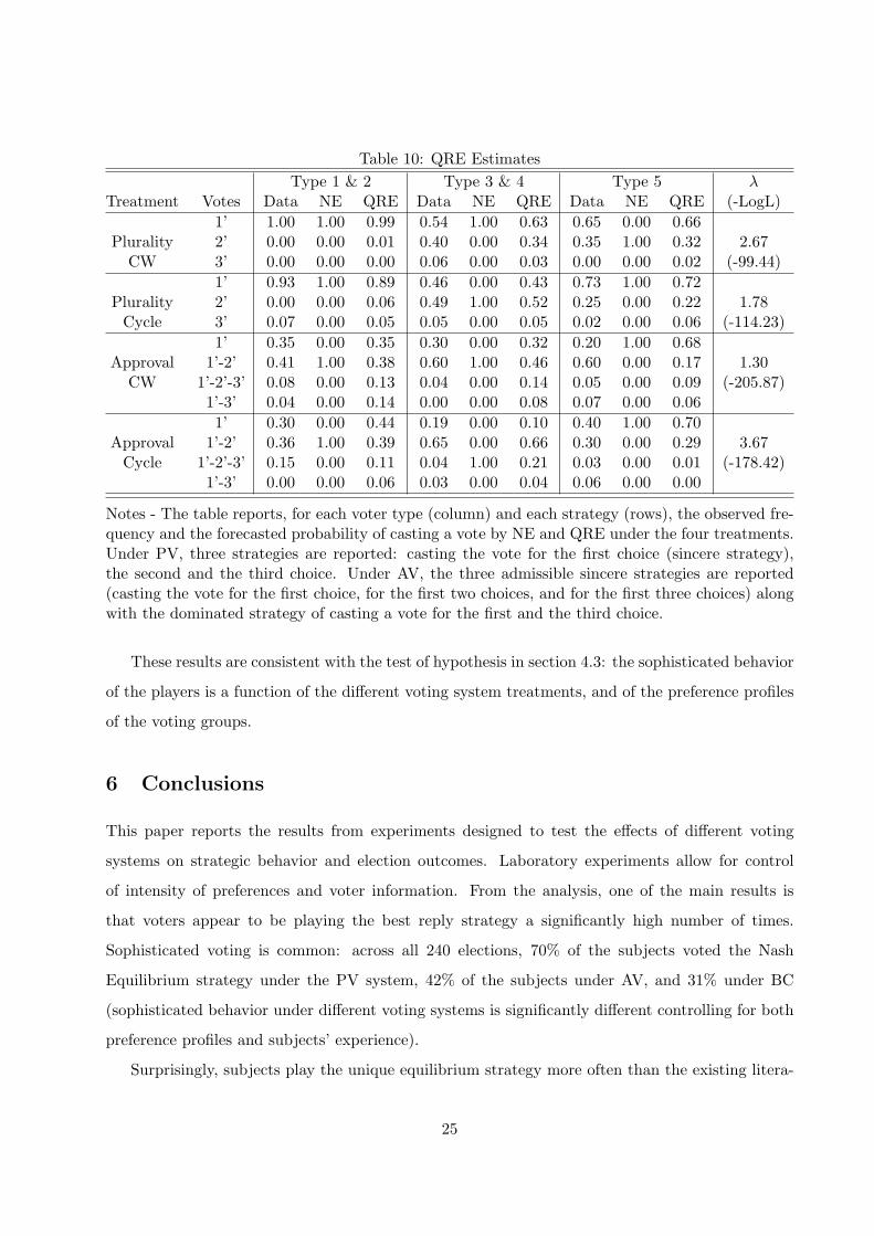
Table 10: QRE EstimatesType 1 & 2 Type 3 & 4 Type 5 λ

Treatment Votes Data NE QRE Data NE QRE Data NE QRE (-LogL)1’ 1.00 1.00 0.99 0.54 1.00 0.63 0.65 0.00 0.66

Plurality 2’ 0.00 0.00 0.01 0.40 0.00 0.34 0.35 1.00 0.32 2.67CW 3’ 0.00 0.00 0.00 0.06 0.00 0.03 0.00 0.00 0.02 (-99.44)

1’ 0.93 1.00 0.89 0.46 0.00 0.43 0.73 1.00 0.72Plurality 2’ 0.00 0.00 0.06 0.49 1.00 0.52 0.25 0.00 0.22 1.78

Cycle 3’ 0.07 0.00 0.05 0.05 0.00 0.05 0.02 0.00 0.06 (-114.23)1’ 0.35 0.00 0.35 0.30 0.00 0.32 0.20 1.00 0.68

Approval 1’-2’ 0.41 1.00 0.38 0.60 1.00 0.46 0.60 0.00 0.17 1.30CW 1’-2’-3’ 0.08 0.00 0.13 0.04 0.00 0.14 0.05 0.00 0.09 (-205.87)

1’-3’ 0.04 0.00 0.14 0.00 0.00 0.08 0.07 0.00 0.061’ 0.30 0.00 0.44 0.19 0.00 0.10 0.40 1.00 0.70

Approval 1’-2’ 0.36 1.00 0.39 0.65 0.00 0.66 0.30 0.00 0.29 3.67Cycle 1’-2’-3’ 0.15 0.00 0.11 0.04 1.00 0.21 0.03 0.00 0.01 (-178.42)

1’-3’ 0.00 0.00 0.06 0.03 0.00 0.04 0.06 0.00 0.00

Notes - The table reports, for each voter type (column) and each strategy (rows), the observed fre-quency and the forecasted probability of casting a vote by NE and QRE under the four treatments.Under PV, three strategies are reported: casting the vote for the first choice (sincere strategy),the second and the third choice. Under AV, the three admissible sincere strategies are reported(casting the vote for the first choice, for the first two choices, and for the first three choices) alongwith the dominated strategy of casting a vote for the first and the third choice.

These results are consistent with the test of hypothesis in section 4.3: the sophisticated behavior

of the players is a function of the different voting system treatments, and of the preference profiles

of the voting groups.

6 Conclusions

This paper reports the results from experiments designed to test the effects of different voting

systems on strategic behavior and election outcomes. Laboratory experiments allow for control

of intensity of preferences and voter information. From the analysis, one of the main results is

that voters appear to be playing the best reply strategy a significantly high number of times.

Sophisticated voting is common: across all 240 elections, 70% of the subjects voted the Nash

Equilibrium strategy under the PV system, 42% of the subjects under AV, and 31% under BC

(sophisticated behavior under different voting systems is significantly different controlling for both

preference profiles and subjects’ experience).

Surprisingly, subjects play the unique equilibrium strategy more often than the existing litera-

25

ture on iterated solvable games would suggest, and subjects also engage in three or more steps of

elimination significantly more often.

It is worth noting that dominated (and insincere) behavior is quite frequent, especially when

the voting system allows for a higher degree of freedom (i.e., when the voter may cast more than

a single vote or rank the alternatives). In fact subjects casted dominated ballots between 10% and

18% of the time under either PV or AV, but these percentages increase to 40%-50% under BC.

Though such actions are labelled “dominated,” they can be interpreted as strategic attempts to

manipulate the elections results, therefore providing greater support to the evidence that subjects

are not “naive.”

Under PV, the experimental outcomes provide support for Duverger’s law, in creating two-

candidate elections races, especially when the subjects are experienced. This result is consistent

with Gerber et al. (1998) and Forsythe et al. (1996), who find support for Duverger’s law creating

two-candidate races. The frequency of Duvergerian races seems to be sensible to the preference

profile of the electorate, as data show that the absence of a Condorcer candidate reduces the

Duverger’s law occurrence.

To analyze the manipulability of the three voting systems, the number of times the experimental

subjects cast an insincere vote that induced a change in the outcome is compared. Three definitions

of sincerity under AV are adopted: the Brams and Fishburn’s (1978, 1983) definition of “admissible

sincerity,” the Merrill’s (1988) definition of “pure sincerity,” and an intermediate definition that

considers all the strategies in the “admissible sincere” set as sincere except the sophisticated one.

Data show how the three different definitions of AV sincere strategy are critical in determining the

level of manipulation to which AV is vulnerable. Under the first definition, AV is almost always

the least manipulated, but when a more restrictive definition is adopted, the level of manipulation

dramatically increases, showing levels of manipulation sometimes larger than BC (which is on

average the most manipulated one).

According to the mild definition of AV “admissible sincerity,” AV displays by far the lowest

level of manipulation. Elsewhere, PV is the system which displays the lowest level of individual

manipulation. This is because under PV, it is not optimal for all the voters to vote insincerely, but

only for the voters who do not support the trailing candidates. Under AV and BC, this is not the

case.

In terms of social efficiency, unexpectedly the PV System performs significantly better than

both AV and BC (producing an outcome 5% more efficient) in the Condorcet Winner treatment,

26

while all voting systems perform equally well in the Cycle treatment (producing a social welfare

equal to 90% of the optimum social welfare). Yet, consistent with the literature, PV is the weakest

performer under Condorcet efficiency, whereas AV and BC perform remarkably well even with a

small electorate. However, in the last three rounds, PV’s performance improves significantly while

the performances of AV and BC decrease.

A Quantal Response analysis shows that the QRE concept fits the experimental data better

than the Nash equilibrium. The estimated value of λ for PV is fairly high under the Condorcet

Winner treatment, meaning that players play the Nash equilibrium strategies. However in the

Cycle treatment, players’ best responses are more affected by noise. This implies that the analysis

of sophisticated behavior is not robust across different preference profiles. The value of the Log

likelihood for AV games is not as high as for PV, meaning that a Quantal response interpretation

does not fit the data as well as under PV. This implies that under AV, voters’ best responses are

more affected by noise. Even here, the difference under the two treatments is significant suggesting

that different strategic environments do matter in the the strategic analysis of voting games.

7 Appendix

7.1 Instructions

You are about to participate in an experimental session on voting procedures and you will be paid

for your participation with a cash voucher privately at the end of the session. What you earn

depends partly on your own decisions, partly on the decisions of others, and partly on chance.

Please turn off pagers and cellular phones now. Please close any programs you may have open on

the computer.

The entire session will take place through computer terminals and all interaction between you

and other session participants will take place through the computers. Please do not attempt to

directly communicate with other participants during the session. If you have any question during

the experiment, ask the experimenter and she will answer them for you. Other than these questions,

you must keep silent until the experiment is completed. If you break silence while the experiment

is in progress, you will be asked to leave the experiment.

27

7.1.1 Voting groups

This experiment will last for 20 periods. In each period you will be placed into groups of 5 people.

You will not be told who else is in your group. You and the other members of your group will be

asked to make a decision in that period. Then the next period you will be placed into new groups

and again asked to make decisions, and so forth, for 20 periods. Thus, in each period the group

memberships will be different from the memberships in previous periods and you will not belong

to the same group more than once.

In each period, the group is asked to choose one alternative among a set of four: A, B, C, and

D. Every member of the group is asked to vote accordingly to the rule discussed in the following

screens. The votes cast will determine the winning alternative in that period.

In each period you may earn some ”experimental points” which will be converted into $, at a

rate of 20 cents for every point, at the end of the experiment.

7.1.2 Types

At the beginning of this experiment each of you will be randomly assigned a type (1, 2, 3, 4 or 5).

The type you are assigned to will remain the same for the entire experiment. Each group will be

composed of one person of each type.

7.1.3 Payoffs

In each round, the payoff you will receive will depend upon the winning alternative in your group.

The Payoff Tables show the payoffs you will receive if any of the four alternatives wins. In the

Payoff Tables you will also find the payoffs that other types of voters will receive depending on

which alternative wins. This means that every member of the group knows the payoffs that the

other members of the group will receive if each of the four alternatives wins.

The payoff schedule will stay the same for 10 periods. At the beginning of the 11th period, the

payoffs will change for all types of voters as shown in the Payoff Table. -Please look at the Payoff

Tables now-

In the Payoff Table you will find two tables. The first one tells you the payoffs that every type

will gain in the first 10 periods (periods: 1 - 10). The second one tells you the payoffs that every

member will get in the last 10 periods (periods: 11 - 20).

28

Period 1-10 A B C D Period 11-20 A B C DType 1 7 5 1 3 Type 1 3 7 1 5Type 2 7 5 1 3 Type 2 3 7 1 5Type 3 3 1 7 5 Type 3 7 1 5 3Type 4 3 1 7 5 Type 4 7 1 5 3Type 5 5 1 3 7 Type 5 3 5 7 1

7.1.4 Example: How to read the table

Let’s take the first table. It tells you the payoffs you and the other members of the group would

receive for every potential winning alternative.

For example, in each of the first ten periods, if alternative C wins, members of type 1 and 2

will get 1 experimental point, members of type 3 and 4 will get 7 points, and members of type 5

will get 3 points. After the 10th round, the payoffs attached to each alternative changes. Now if

alternative C wins, members of types 1 and 2 will get 5 experimental points, members of types 3

and 4 will get 1 point, and members of type 5 will get 7 points.

Whenever a tie occurs between 2 alternatives, each member gets the average of the experimental

points attached to each alternative. For example, in each of the first ten periods, if alternative A

and C tie, members of type 1 and 2 will get 4 experimental points, members of type 3 and 4 will

get 5 points, and members of type 5 will get 4 points.

7.1.5 Voting Rule

If PV treatment.

You may cast only 1 vote for an alternative of your choice. You can change your ballots until you

press the button ”Continue”, but you cannot change the ballot after that. After all the members

of the group have casts their ballots, the number of votes for every alternative will be summed up.

You will be told the total number of votes each alternative receives in your group. The alternative

with the highest number of votes in your group will be the winner of the election in your group. If

two or more alternatives tie with equal (highest) vote totals, your payoff will be the average of the

payoffs you attach to each tying alternative.

If AV treatment.

You may cast only 1 vote for one or more alternatives of your choice. You can change your

ballots until you press the button ”Continue”, but you cannot change the ballot after that. After

all the members of the group have casts their ballots, the number of votes for every alternative will

29

be summed up. You will be told the total number of votes each alternative receives in your group.

The alternative with the highest number of votes in your group will be the winner of the election

in your group. If two or more alternatives tie with equal (highest) vote totals, your payoff will be

the average of the payoffs you attach to each tying alternative.

If BC treatment.

You may cast your ballot by ranking the 4 alternatives from the most preferred to the least

preferred one. A decreasing number of score points will be attached to them starting from 3 points

for your most preferred to 0 points for the least preferred. You can change your ballots until you

press the button ”Continue”, but you cannot change the ballot after that. After all the members of

the group have casts their ballots, the number of score points for every alternative will be summed

up. You will be told the total number of points each alternative receives in your group. The

alternative with the highest number of points in your group will be the winner of the election in

your group. If two or more alternatives tie with equal (highest) points totals, your payoff will be

the average of the payoffs you attach to each tying alternative.

7.1.6 Example: How the voting rule works

If PV treatment.

Let’s suppose that 1 member voted for A; 1 member for B; 1 member for C; and 2 members for

D. D would win, since D received the highest number of votes. The payoffs would be: types 1 and

2 would get 3 experimental points; types 3 and 4 would get 5 points; type 5 would get 7 points

7.2 Tables of experimental results

30

Table A1: Voters’ behavior in CW treatment.Plurality Approval Voting Borda

Sinc Soph Dom Sinc Soph Dom Sinc Soph DomPooled 1.00 0.00 0.43 0.41 0.16 0.39 0.61

(0.00) (0.00) (0.22) (0.23) (0.19) (0.13) (0.13)

1&2 Non Exp 1.00 0.00 0.53 0.43 0.04 0.35 0.65(0.00) (0.00) (0.25) (0.29) (0.16) (0.13) (0.13)

Exp 1.00 0.00 0.33 0.39 0.28 0.43 0.57(0.00) (0.00) (0.12) (0.17) (0.14) (0.12) (0.12)

Pooled 0.54 0.46 0.34 0.60 0.06 0.34 0.08 0.58(0.26) (0.26) (0.23) (0.25) (0.11) (0.23) (0.12) (0.25)

3&4 Non Exp 0.55 0.45 0.28 0.63 0.09 0.30 0.03 0.67(0.26) (0.26) (0.25) (0.32) (0.13) (0.28) (0.08) (0.29)

Exp 0.53 0.47 0.40 0.57 0.03 0.38 0.13 0.49(0.28) (0.28) (0.21) (0.17) (0.08) (0.18) (0.13) (0.17)

Pooled 0.65 0.35 0.00 0.65 0.20 0.15 0.40 0.60(0.40) (0.40) (0.00) (0.37) (0.25) (0.24) (0.21) (0.21)

5 Non Exp 0.55 0.45 0.00 0.55 0.25 0.20 0.30 0.70(0.37) (0.37) (0.00) (0.37) (0.26) (0.26) (0.26) (0.26)

Exp 0.75 0.25 0.00 0.75 0.15 0.10 0.50 0.50(0.42) (0.42) (0.00) (0.35) (0.24) (0.21) (0.00) (0.00)

Notes - The table reports the average frequency with which voters play sincere, sophisticated, anddominated strategies under different voting systems (columns). Standard deviations are in paren-thesis. For each type of voter (row), three statistics are given respectively for pooled subjects, forthe non experienced subjects, and for the experienced subjects (who experienced a early treatment).

31

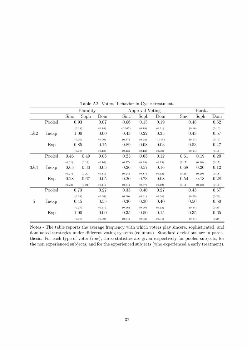
Table A2: Voters’ behavior in Cycle treatment.Plurality Approval Voting Borda

Sinc Soph Dom Sinc Soph Dom Sinc Soph DomPooled 0.93 0.07 0.66 0.15 0.19 0.48 0.52

(0.14) (0.14) (0.365) (0.19) (0.21) (0.16) (0.16)

1&2 Inexp 1.00 0.00 0.43 0.22 0.35 0.43 0.57(0.00) (0.00) (0.37) (0.22) (0.175) (0.17) (0.17)

Exp 0.85 0.15 0.89 0.08 0.03 0.53 0.47(0.18) (0.18) (0.13) (0.12) (0.08) (0.14) (0.14)

Pooled 0.46 0.49 0.05 0.23 0.65 0.12 0.61 0.19 0.20(0.31) (0.29) (0.10) (0.27) (0.29) (0.13) (0.17) (0.16) (0.17)

3&4 Inexp 0.65 0.30 0.05 0.26 0.57 0.16 0.68 0.20 0.12(0.27) (0.20) (0.11) (0.24) (0.17) (0.12) (0.21) (0.20) (0.18)

Exp 0.28 0.67 0.05 0.20 0.73 0.08 0.54 0.18 0.28(0.22) (0.24) (0.11) (0.31) (0.37) (0.12) (0.11) (0.12) (0.14)

Pooled 0.73 0.27 0.33 0.40 0.27 0.43 0.57(0.38) (0.38) (0.30) (0.31) (0.34) (0.29) (0.29)

5 Inexp 0.45 0.55 0.30 0.30 0.40 0.50 0.50(0.37) (0.37) (0.26) (0.26) (0.32) (0.24) (0.24)

Exp 1.00 0.00 0.35 0.50 0.15 0.35 0.65(0.00) (0.00) (0.34) (0.33) (0.34) (0.34) (0.34)

Notes - The table reports the average frequency with which voters play sincere, sophisticated, anddominated strategies under different voting systems (columns). Standard deviations are in paren-thesis. For each type of voter (row), three statistics are given respectively for pooled subjects, forthe non experienced subjects, and for the experienced subjects (who experienced a early treatment).

32

References

Besley, Timothy J. and Stephen Coate. (1997). “An Economic Model of Representative Democracy.”

Quarterly Journal of Economics 112: 85–114.

Brams, Steven J. and Peter C. Fishburn. (1978). “Approval Voting.” American Political Science

Review 72(3): 831–47.

Brams, Steven J. and Peter C. Fishburn. (1983). “Approval Voting.” Boston: Birkhuser.

Brams, Steven J. (1994). “Voting procedures.” Handbook of Game Theory. ed. by Aumann, R.J.,

Hart, S. Elsevier. 2.

Cox, Gary W. (1994). “Strategic Voting Equilibria Under the Single Nontransferable Vote.” The

American Political Science Review 88(3): 608–21.

De Sinopoli, Francesco and Alessandro Turrini. (2002). “A Remark on Voter Rationality in a Model

of Representative Democracy.” Journal of Public Economic Theory 4(2): 163–70.

Duverger, Maurice. (1954). Political Parties: Their Organization and Activity in the Modern State.

Wiley, New York.

Farquharson, Robin. (1969). Theory of Voting . Yale Univ. Press, New Haven.

Feddersen, Timothy and Wolfgang Pesendorfer. (1997). “Voting Behavior and Information Aggre-

gation in Elections with Private Information.” Econometrica 65(5): 1029–58.

Fiorina, Morris and Charles R. Plott. (1978). “Committee Decisions Under Majority Rule: An

Experimental Study.” American Political Science Review 72: 575–98.

Fischbacher, Urs. (1999). z-Tree - Zurich Toolbox for Readymade Economic Experiments - Ex-

perimenter’s Manual . Working Paper Nr. 21, Institute for Empirical Research in Economics,

University of Zurich.

Forsythe, Robert, Roger B. Myerson, Thomas A. Rietz, and Robert J. Weber. (1996). “An Experi-

mental Study of Voting Rules and Polls in Three-Candidate Elections.” International Journal

of Game Theory 25(3): 355–83.

Gale, David. (1953). “A Theory of N-Person Games With Perfect Information.” Proceedings of the

National Academy of Sciences 39: 496–501.

33

Gerber, Elisabeth A., Rebecca B. Morton, and Thomas A. Rietz. (1998). “Minority Representation

in Multimember Districts.” American Political Science Review 92: 127–44.

Gibbard, Allan. (1973). “Manipulation of Voting Schemes: a General Result.” Econometrica 41(4):

587–601.

Harsanyi, John C. (1977). Rational Behavior and Bargaining Equilibrium in Games and Social

Situations. Cambridge: Cambridge University Press.

Luce, Duncan R. and Howard Raiffa. (1957). Games and Decisions. Wiley, New York

McKelvey, Richard D. (1976). “Intransitivities in Multidimensional Voting Models and Some Im-

plications for Agenda Control.” Journal of Economic Theory 12: 472–82.

McKelvey, Richard D. (1979). “General Conditions for Global Intransitivities in Formal Voting

Models.” Econometrica 47: 1085–1112.

McKelvey, Rihard D. and Thomas R. Palfrey. (1995). “Quantal Response Equilibria for Normal

Form Games.” Games and Economic Behavior 10: 6–38.

Merrill, Samuel III. (1984). “A Comparison of Efficiency of Multicandidate Electoral Systems”

American Journal of Political Science 28(1): 23–48.

Merrill, Samuel III. (1988). Making Multi-candidate Elections More Democratic Princeton NJ:

Princeton University Press.

Moreno Diego and John Wooders. (1996). “Coalition-Proof Equilibrium.” Games and Economic

Behavior 17: 80–112.

Myerson, Roger B. and Robert J. Weber. (1993). “A theory of Voting Equilibria.” American

Journal of Political Science 87(1): 102–14.

Nagel, Rosemarie. (1995). “Unraveling in guessing games: an experimental study.” American

Economic Review 85: 1313–26.

Nagel, Rosemarie. (1999). “A survey of experimental guessing games: a study of bounded rationality

and learning.” In: Budescu, Erev, and Zwick. (Eds.), Games and Human Behavior: Essays in

Honor of Amnon Rapoport. 105–42.

34

Niemi, Richard G. (1984). “The Problem of Strategic behavior under Approval Voting.” American

Political Science Review 78: 952–958.

Palfrey, Thomas R. (1989). “A Mathematical Proof of Duverger’s Law.” Models of Strategic Choice

in Politics. Ed. by P. C. Ordeshook.University of Michigan Press, Ann Arbor. 69–92.

Plott, Charles R. (1967). “A Notion of Equilibrium Under Majority Rule.” American Economic

Review 57: 787–806.

Rajan, Uday. (1998). “Trembles in the Bayesian Foundations of Solution Concepts of Games.”

Journal of Economic Theory 82: 248–266.

Saari, Donald G. (1989). “A Dictionary for Voting Paradoxes.” Journal of Economic Theory 48:

443–475.

Satterthwaite, Mark Allen. (1975). “Strategy Proofness and Arrow’s Conditions: Existence and

Correspondence Theorems for Voting Procedures and Social Welfare Functions.” Journal of

Economic Theory 10(2): 187–207.

Schofield, Norman. (1983). “Generic Instability of Majority Rule.” Review of Economic Studies 50:

695–705.

Smith, David A. (1999). “Manipulability measures of common social choice functions.” Social

Choice and Welfare 16(4): 639–661.

35