visualization of oxidative stress in ex vivo biopsies
TRANSCRIPT

Visualization of oxidative stress in ex vivo
biopsies using electron paramagnetic resonance
imaging
Håkan Gustafsson, Martin Hallbeck, Mikael Lindgren, Natallia Kolbun, Maria Jonson, Maria
Engström, Ebo de Muinck and Helene Zachrisson
Linköping University Post Print
N.B.: When citing this work, cite the original article.
Original Publication:
Håkan Gustafsson, Martin Hallbeck, Mikael Lindgren, Natallia Kolbun, Maria Jonson, Maria
Engström, Ebo de Muinck and Helene Zachrisson, Visualization of oxidative stress in ex vivo
biopsies using electron paramagnetic resonance imaging, 2015, Magnetic Resonance in
Medicine, (73), 4, 1682-1691.
http://dx.doi.org/10.1002/mrm.25267
Copyright: Wiley
http://eu.wiley.com/WileyCDA/
Postprint available at: Linköping University Electronic Press
http://urn.kb.se/resolve?urn=urn:nbn:se:liu:diva-113407
1
Visualisation of oxidative stress in ex vivo biopsies using electron paramagnetic resonance imaging
(EPRI)
H. Gustafsson1, 2, *, M. Hallbeck3, M. Lindgren4, 5, N. Kolbun1, 2, M. Jonson5, M. Engström1, 2, E. de
Muinck6, H. Zachrisson6
1. Department of Medical Technology (MTÖ), Radiation Physics, Department of Medicine and
Health Sciences, Linköping University, Linköping, Sweden
2. Center for Medical Image Science and Visualization (CMIV), Linköping University, Sweden.
3. Department of Clinical Pathology and Clinical Genetics, and Department of Clinical and
Experimental Medicine, Linköping University, Linköping, Sweden.
4. Department of Physics, Norwegian University of Science and Technology, Trondheim, Norway.
5. IFM-Department of Chemistry, Linköping University, Linköping, Sweden.
6. Department of Medical and Health Sciences (IMH), Division of Cardiovascular Medicine,
Linköping University, Sweden.
* Corresponding author.
Contact details:
E-mail: [email protected]
Address: Håkan Gustafsson, IMH/Radiation Physics, Linköping University, 581 85 Linköping,
Sweden
Telephone: +46 (0)10 104 3023 or +46 (0)709 428446
Fax: Not available
Word count: 4314

2
ABSTRACT
Purpose
The purpose of this study was to develop an X-Band electron paramagnetic resonance imaging (EPRI)
protocol for visualisation of oxidative stress in biopsies.
Methods
The developed EPRI protocol was based on spin trapping with the cyclic hydroxylamine spin probe 1-
hydroxy-3-methoxycarbonyl-2,2,5,5-tetramethylpyrrolidine (CMH) and X-Band EPR imaging.
Computer software was developed for deconvolution and back-projection of the EPR image. A
phantom containing radicals of known spatial characteristic was used for evaluation of the developed
protocol. As a demonstration of the technique EPRI of oxidative stress was performed in six sections
of atherosclerotic plaques. Histopathological analyses were performed on adjoining sections.
Results
The developed computer software for deconvolution and back-projection of the EPR images could
accurately reproduce the shape of a phantom of known spatial distribution of radicals. The developed
protocol could successfully be used to image oxidative stress in six sections of the three ex vivo
atherosclerotic plaques.
Conclusion
We have shown that oxidative stress can be imaged using a combination of spin trapping with the
cyclic hydroxylamine spin probe CMH and X-Band EPR imaging. A thorough and systematic
evaluation on different types of biopsies must be performed in the future to validate the proposed
technique.
Key Words: EPR, EPR imaging, EPRI, spin trap, oxidative stress, reactive oxygen species
3
INTRODUCTION
Overproduction of reactive oxygen species (ROS) such as superoxide radicals (O2•-) and hydroxyl
radicals (OH•) can lead to oxidative stress with subsequent oxidative damage to tissues. ROS are also
known to be important for physiological functions such as for elimination of pathogens and as cell
signalling molecules (1-2). It is well-known that ROS are involved in the pathology of a large number
of diseases (3) and it has been shown that oxidative stress is a key factor in the initiation and
progression of atherosclerosis (4) in the development of endothelial dysfunction (5) and hypertension
(6).
Measurement of radicals in human tissues is a methodological challenge because of high reactivity
and short half-life of reactive oxygen and nitrogen species which leads to difficulties for direct
determination. Electron paramagnetic resonance imaging (EPRI) is a technique for imaging of
paramagnetic species (7) and provides a unique possibility to image the distribution of free radicals in
medical samples. EPRI is being developed towards in vivo monitoring and imaging of radicals in
mice (8-10) and initial attempts of in vivo EPR in humans have been conducted (11-12).
EPRI has several similarities with (nuclear) magnetic resonance imaging (MRI), but the progress of
EPRI has been slow compared to MRI. This is partly due to several technical difficulties associated
with the often very low concentrations of paramagnetic species in the samples of interest and the fast
electronic relaxation times. (T1 is typically in the order of milliseconds to seconds for protons as
compared to 1 to 20 microseconds for electrons (13)). The development of pulsed EPRI methods has
therefore been hindered and EPRI is therefore typically performed using filtered back-projection of a
set of repeated continuous wave (c. w.) experiments for different combination of gradient angles (14-
15). However, recent progress of EPR imaging is promising and may open for a large number of
important clinically applications. Nevertheless, visualisation of oxidative stress in biopsies and in vivo
needs to be further developed.
Visualisation of radicals using EPRI is based on the local interaction between the tissue and molecular
probes (EPR spin traps/probes)(16-17). Two main techniques can be used: (1) The rate constant (half-
life) of the reduction of a nitroxide free radical to an EPR silent diamagnetic hydroxylamine has been
observed in comparisons of images obtained at different time after the incubation/injection with the
nitroxide free radical. The rate constant of the reduction of the nitroxide free radical is dependent on
the tissue redox status and the time dependent loss of signal in the images can be used to assess tissue
redox status. Rapid loss of signal as compared to normal tissue thus indicates that the tissue is highly
4
reducing compared to normal tissue. There are examples in literature such as in the incubation with
TEMPO (2,6,6-Tetramethylpiperidine-1-oxyl) for studies of UV-induced ROS in human skin biopsies
(18)) and injection of 3-CP (3-carbamoyl-2,2,5,5-tetramethylpyrrolidine-N-oxyl) in mice for imaging
of tumour redox status (19)). Another method (2) for imaging of ROS is the incubation or injection of
an EPR silent diamagnetic cyclic hydroxylamine. The diamagnetic cyclic hydroxylamine will react
with ROS and accumulate as a free radical in regions containing high concentrations of ROS. This
will be observed as regions with high signal intensity. While cyclic hydroxylamines (20-21) has been
shown to be especially useful for detection of ROS in cardiovascular studies (22), to the best of our
knowledge no one has used the combination of EPR imaging with EPR silent diamagnetic cyclic
hydroxylamines for imaging of oxidative stress with high signal intensity in regions with oxidative
stress as we demonstrate here.
The diamagnetic cyclic hydroxylamine spin probe 1-hydroxy-3-methoxycarbonyl-2,2,5,5-
tetramethylpyrrolidine (CMH) is known to react with superoxide, peroxyl radical, nitrogen dioxide
and peroxynitrite (but do not react with H2O2 or nitric oxide) (20, 23-24). The oxidation of CMH
leads to the formation of the paramagnetic 3-methoxycarbonyl-proxyl nitroxide (CM•) (24) and it is
known that a majority of the formed CM• in vitro and in vivo is due to oxidation of CMH by
superoxide (25-26).
Vulnerable atherosclerotic plaques are prone to rupture and frequently lead to stroke or myocardial
infarction. Vulnerable plaques are characterized by an increased number of inflammatory cells such as
macrophages and related inflammation, especially in the cap, might lead to cap rupture as well as
thrombus formation. High local concentrations of immune cells such as macrophages are correlated to
regions of high oxidative stress (27) and it has been hypothesized that this leads to increased activity
of matrix metalloproteinase which degrades the fibrous cap and therefore further destabilise the cap of
atherosclerotic plaques with subsequent risk of cap rupture (28).
The aim of this work was to develop a new method and an imaging protocol for imaging of ROS in
biopsies. The method was based on incubation with an EPR silent diamagnetic cyclic hydroxylamine
and observing high signal intensity in regions with possible high oxidative stress using X Band EPR
imaging. The developed protocol was demonstrated for imaging of ROS in six sections of three
symptomatic ex vivo atherosclerotic plaques (two sections from each plaque).
METHODS
EPRI phantom

5
An EPRI phantom was made using 1.82 g gelatine leafs (gelatine from animal origin, Dr. Oetker,
Mölndal, Sweden), which were dissolved in 0.35 dl water with 1 mM TEMPO (2,2,6,6-Tetramethyl-
1-piperidinyloxy) (Aldrich 214000-5G) in a beaker using a magnetic stirrer/heater until completely
dissolved. An EPR tissue cell (WG-806-A-Q-P Suprasil tissue cell, Wilmad-LabGlas, Vineland, New
Jersey, USA) was completely filled with the gelatine/TEMPO mixture and the gelatine was allowed to
solidify completely at 4 °C. The gelatine with TEMPO could thereafter be cut into desired shapes and
sizes. A 6 mm diameter circle was used as the EPRI phantom to be reproduced in the imaging
reconstruction software as discussed below.
Patient data and duplex ultrasound in vivo
Three patients (a woman 64 years old, a man 74 years old and a man 85 years old) undergoing carotid
endarterectomy (CEA) was prospectively enrolled for study participation. The study was approved by
the Local Ethical Review Board in Linköping, Sweden. The participants were both written and
verbally informed about the purpose of the study and provided their written informed consent to
participate. All patients had symptomatic internal carotid artery (ICA) stenosis [minor stroke n = 2;
transient ischemic attack (TIA), n = 1]. Preoperative duplex ultrasound of the neck vessels was
performed within one week before carotid endarterectomy at an angle of 60 degrees at maximum
between the transducer and the blood flow direction using a high frequency ultrasound Acuson S2000
scanner (Siemens, Mountain View, USA) equipped with a 9 MHz -18 MHz transducer. Ultrasound
images/data were saved for further offline analysis using computerized image analysis software;
Adobe Photoshop CS5 (Adobe systems, Mountain View, USA). The degree of internal carotid artery
stenosis was measured as an evaluation of the peak systolic flow velocity (PSV), i.e. the European
Carotid Surgery Trial (ECST) method (29). Plaque composition and cap surface were objectively
assigned.
Carotid endarterectomy, plaque transport and storage
Immediately after carotid endarterectomy the plaque was placed in a small plastic bottle and snap-
frozen in liquid nitrogen. The plaque was transported to the EPRI laboratory and stored for up to 19
days in liquid nitrogen until the time of cryosection and subsequent EPRI.
Spin trap solution
0.01 M, pH = 7.4 phosphate buffered saline (PBS) (Sigma P3813-10-PAK) with 100 µM diethylene
triamine pentaacetic acid (DTPA) (Sigma-Aldrich D6518-5G) was kept on ice and bubbled with
nitrogen gas for approximately 30 minutes prior to addition of CMH (1-hydroxy-3-methoxycarbonyl -
2,2,5,5-tetramethylpyrrolidine) (Noxygen Science Transfer & Diagnostics GmbH. NOX-02.1-50mg)
to a final concentration of 30 mM CMH. This spin trap solution was kept on ice and under constant
6
bubbling with nitrogen gas until incubation of carotid plaque slices (see section below) to ensure an
oxygen free environment.
Cryosection
The plaques were equilibrated to – 20 °C for 90 minutes in a MICROM HM 550 Cryostat (MICROM
International GmbH, Walldorf, Germany) before mounted to a sample plate using Tissue-Tek O.C.T
compound (Histolab, Göteborg, Sweden). Cryosectioning was performed at – 20 °C chamber
temperature, with a knife temperature of – 17 °C. Histology slices for Hematoxylin and Eosine
staining (H&E) were cut with a thickness of 20 µm, while slices for EPRI had a thickness of 250 µm.
The slices for H&E staining were placed on SuperFrost Plus slides ( Menzel-Gläser, Braunschweig,
Germany), dried at room temperature for 30 minutes and stored at – 20 °C until use. Slices for EPRI
were placed on an EPRI tissue cell and immediately transported to the EPRI laboratory.
Incubation with spin trap and tissue cell.
Immediately after cryosection the 250 µm slices for EPRI were placed on the EPRI tissue cell and
transported to the EPRI laboratory. Time for transport was approximately 2 minutes, which allowed
the samples to thaw slightly. Incubation was performed using 30 µL of the spin trap solution (see
section above) during exactly three minutes and thereafter all surplus of the solution was gently
removed using a piece of paper on the sides of the plaques. Incubated plaques were thereafter covered
using Parafilm (Pechiney Plastic Packaging Company, Chicago, IL) to avoid drying and deterioration
of the biopsy.
EPRI
EPRI was performed using an X Band (9.6 GHz) Bruker E540 EPR and EPR imaging spectrometer
(Bruker BioSpin GmbH, Rheinstetten, Germany) equipped with a E540 GC2X two axis X band
gradient coil set with gradients along y axis (along sample tube) and z axis (along B0). An ER
4108TMHS resonator was used suitable for the 25 mm air gap between the gradient coils. All
measurements were performed in room temperature. During measurements, the samples were placed
on the WG-806-A-Q-P Suprasil tissue cell. An EPR spectrum obtained without gradients was
obtained for the deconvolution (see section below) using the following parameters: applied
microwave power 10.02 mW, modulation amplitude 0.150 mT, modulation frequency 100.0 kHz,
sweep width 15.94 mT, points 512, sweep time: 10.01 s, time constant 10.24 ms, number of
accumulated scans 5. EPRI was performed using the same parameters as for EPR spectroscopy with
the addition of the following imaging specific parameters: field of view (FOV): 14.00 mm * 14.00
mm, gradient strength (G) 3.000 mT/cm, pixel size 0.500 mm * 0.500 mm, first gradient angle
4.286 °, number of gradient angles 21, spectrum width 5.000 mT. The paramagnetic 3-
7
methoxycarbonyl-proxyl nitroxide (CM•) is very stable compared to the measurement time used in
the present study (22) and the total measurement time was therefore of less importance. However,
there is a constant, but slow, increase of CM• in regions with e.g. superoxide and the acquisition time
was therefore limited to 25 minutes to keep an approximately constant signal-to-noise ratio during
acquisition.
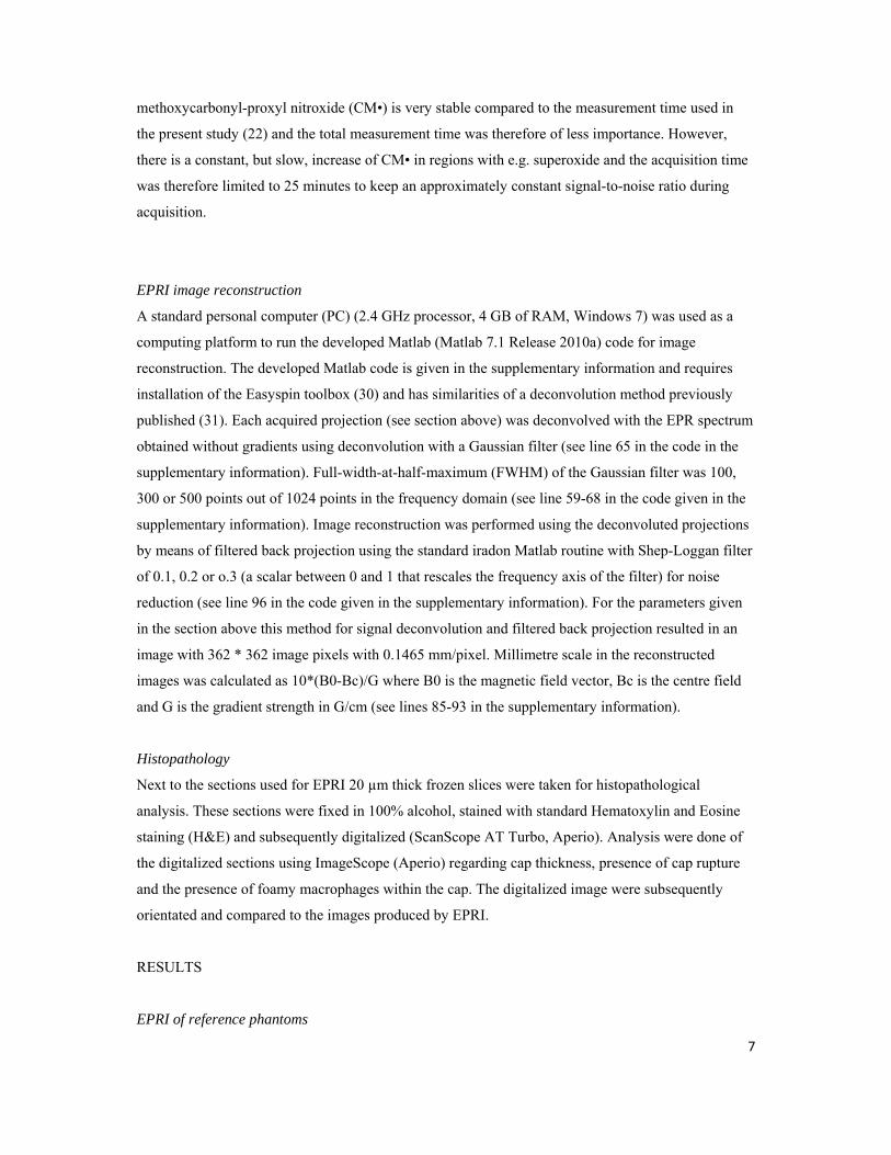
EPRI image reconstruction
A standard personal computer (PC) (2.4 GHz processor, 4 GB of RAM, Windows 7) was used as a
computing platform to run the developed Matlab (Matlab 7.1 Release 2010a) code for image
reconstruction. The developed Matlab code is given in the supplementary information and requires
installation of the Easyspin toolbox (30) and has similarities of a deconvolution method previously
published (31). Each acquired projection (see section above) was deconvolved with the EPR spectrum
obtained without gradients using deconvolution with a Gaussian filter (see line 65 in the code in the
supplementary information). Full-width-at-half-maximum (FWHM) of the Gaussian filter was 100,
300 or 500 points out of 1024 points in the frequency domain (see line 59-68 in the code given in the
supplementary information). Image reconstruction was performed using the deconvoluted projections
by means of filtered back projection using the standard iradon Matlab routine with Shep-Loggan filter
of 0.1, 0.2 or o.3 (a scalar between 0 and 1 that rescales the frequency axis of the filter) for noise
reduction (see line 96 in the code given in the supplementary information). For the parameters given
in the section above this method for signal deconvolution and filtered back projection resulted in an
image with 362 * 362 image pixels with 0.1465 mm/pixel. Millimetre scale in the reconstructed
images was calculated as 10*(B0-Bc)/G where B0 is the magnetic field vector, Bc is the centre field
and G is the gradient strength in G/cm (see lines 85-93 in the supplementary information).
Histopathology
Next to the sections used for EPRI 20 µm thick frozen slices were taken for histopathological
analysis. These sections were fixed in 100% alcohol, stained with standard Hematoxylin and Eosine
staining (H&E) and subsequently digitalized (ScanScope AT Turbo, Aperio). Analysis were done of
the digitalized sections using ImageScope (Aperio) regarding cap thickness, presence of cap rupture
and the presence of foamy macrophages within the cap. The digitalized image were subsequently
orientated and compared to the images produced by EPRI.
RESULTS
EPRI of reference phantoms

8
The imaging protocol was calibrated and evaluated using a phantom of known size and shape. This
was particularly important to be able to obtain precise geometrical parameters of the measured
heterogeneous radical distribution in unknown biological samples. Thus, a phantom (Figure 2, Panel
A) was constructed from gelatine containing 1 mM TEMPO to verify the image reconstruction using a
well-defined sample with high enough signal-to-noise ratio. While the EPRI spectrometer used for
this work allows gradient strengths up to 17 mT/cm, the imaging experiments described here were
performed using a modest gradient strength (G) of only 3 mT/cm. The reason for this was that
preliminary experiments had showed that 3 mT/cm was optimal for the limited signal intensity
available from incubated sections of atherosclerotic plaques. Even though higher gradient strengths
give the theoretical possibility of increased image resolution, it is necessary to have high enough
signal-to-noise ratio to be able to perform a successful deconvolution process.
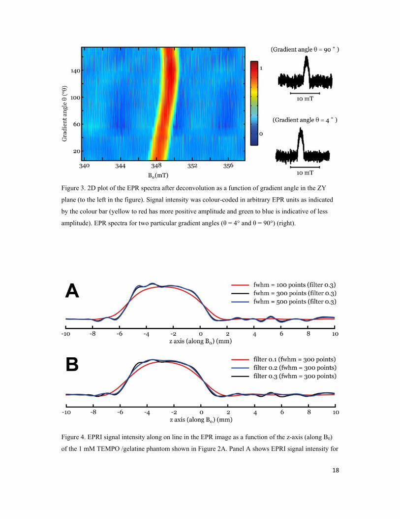
For this sample EPR spectra after deconvolution as a function of gradient angle in the ZY plane are
shown in Figure 3. The left panel is a 2D plot showing the EPR spectra after deconvolution as a
function of gradient angle, color-coded so that yellow to red is more positive amplitude and green to
blue is less amplitude. Representative EPR spectra after deconvolution for two particular gradient
angles (θ = 4° and θ = 90°) are shown in the right panel.
The developed software (described in the experimental section above and in the supplementary
information) was tested for image reconstruction of phantoms with radical distributions of known
sizes and shapes. As an example we show the analysis of the phantom shown in Figure 2A: We
studied the impact of the filter parameter used in the Gaussian deconvolution and the Shepp-Logan
filter parameter used in the filtered back-projection on the signal-to-noise ratio and resolution along
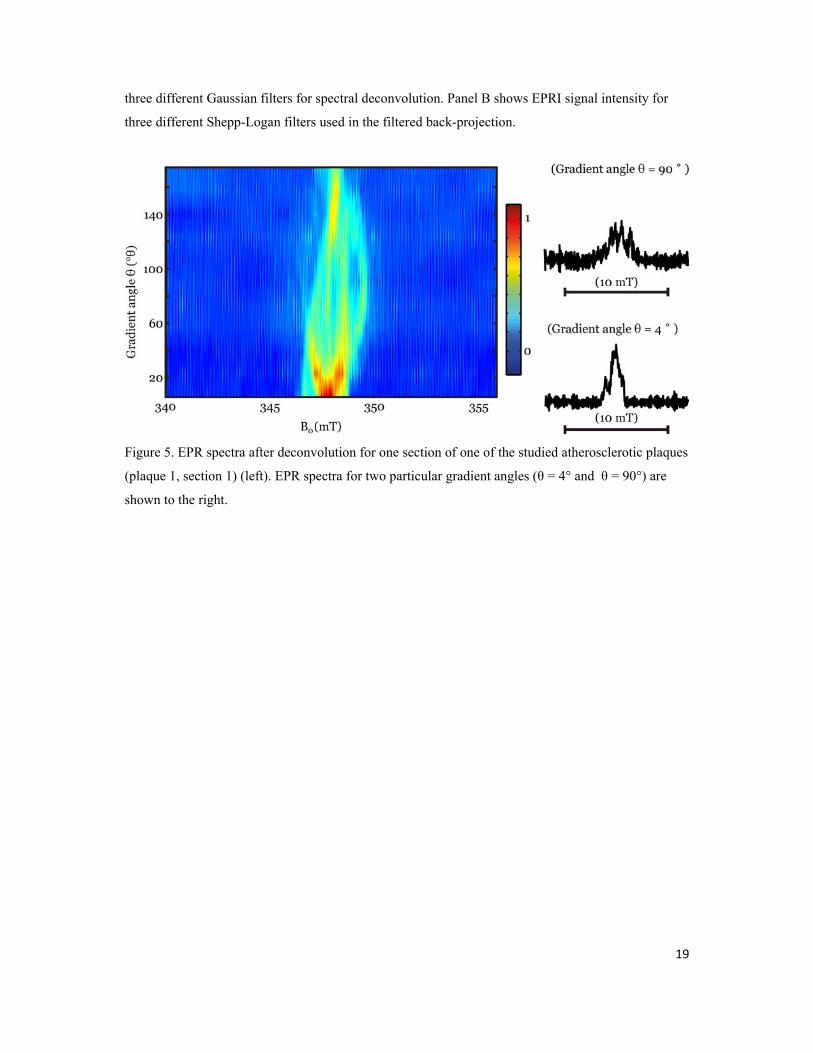
the horizontal axis of the phantom shown in Figure 2. In Figure 4, Panel A, the EPRI signal intensity
is showed for one line along the horizontal axis in the centre of the circular phantom for different
settings of the Gaussian filter used in the deconvolution (for an constant Shepp-Logan filter parameter
in the back-projection). A Gaussian filter with 100 points gave high signal-to-noise ratio but limited
resolution (red curve in Figure 4A). Resolution was increased with increased number of points in the
Gaussian filter (blue and black curves in Figure 4, Panel A), however, at the expense of lower signal-
to-noise ratio. We conclude by trial and errors that 300 points in the Gaussian filter for deconvolution
is a good compromise between resolution and signal-to-noise ratio. Similarly; the Shepp-Logan filter
used in the filtered back-projection (section 2.8), was optimised by trial and error (Figure 4B) and it
was found that a filter of 0.3 was optimal for best resolution without compromising the signal to noise
ratio. As can be read from the z-axis, in all cases of filter testing, the radical distribution is well
contained within the 6 mm diameter of the phantom. Using the optimized filter parameters for
deconvolution and filtered back-projection, reconstruction the EPRI of the gelatine phantom could be

9
calculated as shown in Figure 2 (Figure 2, Panel B) (image reconstruction using fwhm = 300 points
for the Gaussian filter in the deconvolution and a Shepp-Logan filter of 0.3 in the filtered back-
projection). Figure 2, Panel C shows a semi-transparent EPRI-image overlaid on the photograph of
the phantom. As can been seen in Figure 2, Panel A the shape of the phantom was no perfectly
cylindrical and a close examination also revealed that the thickness of the gelatine/TEMPO was not
perfectly uniform. However, there was a good agreement between the distribution of free radicals and
the shape and size of the phantom.
Patient data and duplex ultrasound in vivo
In vivo duplex ultrasound showed that the plaque composition was atheromatous in one plaque and
atheromatous with extensive calcification in two cases. The cap was classified as extensively
ulcerated in all three plaques. The degrees of the internal carotid artery (ICA) stenosis measured as
peak systolic flow velocities (PSV) were 5.3 m/s, 7.0 m/s and 3.0 m/s respectively indicating high
grade stenosis 80 % - 99 % on the ipsilateral (symptomatic) side (ECST (32)).
EPRI of atherosclerotic plaques
Having verified the image reconstruction algorithm, EPRI was performed for totally six sections
(N=6) from the three atherosclerotic plaques (two separated sections from each of the three patients).
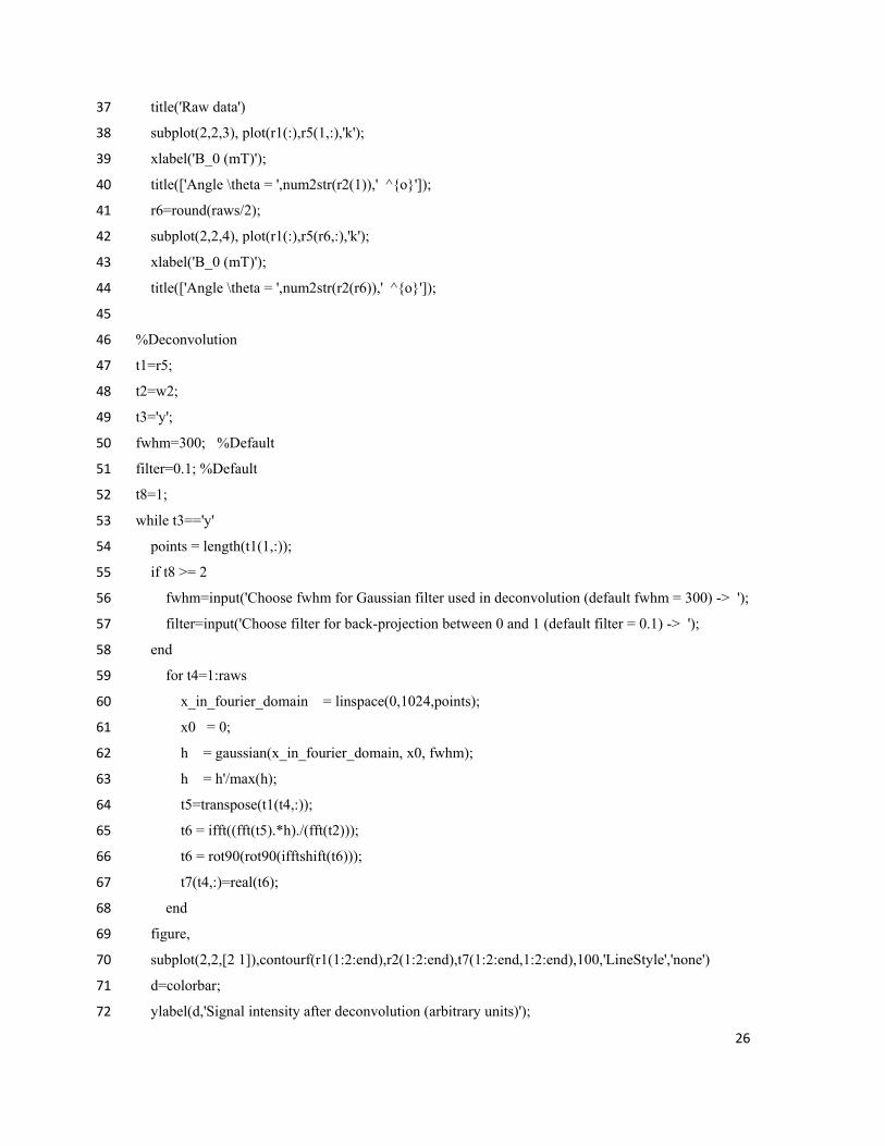
A typical example is shown in Figure 5 and 6 (plaque 1, section 1) where the deconvoluted EPR
spectra as a function of gradient angle are shown in Figure 5 (left panel) and the associated
deconvoluted EPR spectra for two particular gradient angles (θ = 4° and θ = 90°) are shown in Figure
5 (right panel). As shown, the EPR signal was relatively strong with good signal to noise ratio and
there were no problems to reconstruct the free-radical concentration map from these raw data.
Figure 6 shows a photograph of the section (plaque 1, section 1) located on the EPR tissue cell
immediately after cryosection, incubation with spin trap and after covering with Parafilm (Panel A).
Panel B shows the EPRI image obtained after reconstruction of the data shown in Figure 5. Note that
most part of the plaque gives some EPRI intensity but certain areas shows high concentration of spin
probe signal. Panel C shows the areas with highest EPRI intensity fused onto the photograph. Panel D
shows the immunohistochemistry of an adjacent slice of which the slice where the EPRI was carried
out. It is emphasized that this is not the identical sample and that the section is somewhat displaced in
relation with the section used for EPRI, that was mounted on an EPR tissue cell. Despite these small
discrepancies one can easily identify the important regions and carry out immunohistochemistry to be
further discussed below.
10
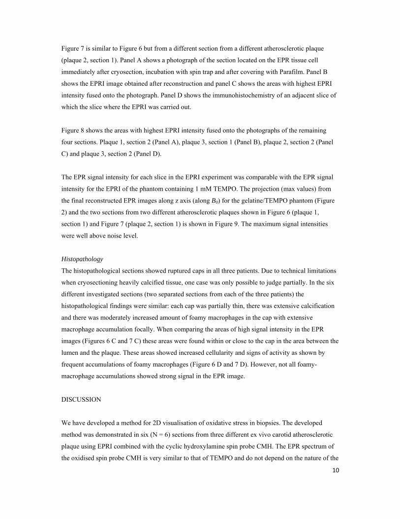
Figure 7 is similar to Figure 6 but from a different section from a different atherosclerotic plaque
(plaque 2, section 1). Panel A shows a photograph of the section located on the EPR tissue cell
immediately after cryosection, incubation with spin trap and after covering with Parafilm. Panel B
shows the EPRI image obtained after reconstruction and panel C shows the areas with highest EPRI
intensity fused onto the photograph. Panel D shows the immunohistochemistry of an adjacent slice of
which the slice where the EPRI was carried out.
Figure 8 shows the areas with highest EPRI intensity fused onto the photographs of the remaining
four sections. Plaque 1, section 2 (Panel A), plaque 3, section 1 (Panel B), plaque 2, section 2 (Panel
C) and plaque 3, section 2 (Panel D).
The EPR signal intensity for each slice in the EPRI experiment was comparable with the EPR signal
intensity for the EPRI of the phantom containing 1 mM TEMPO. The projection (max values) from
the final reconstructed EPR images along z axis (along B0) for the gelatine/TEMPO phantom (Figure
2) and the two sections from two different atherosclerotic plaques shown in Figure 6 (plaque 1,
section 1) and Figure 7 (plaque 2, section 1) is shown in Figure 9. The maximum signal intensities
were well above noise level.
Histopathology
The histopathological sections showed ruptured caps in all three patients. Due to technical limitations
when cryosectioning heavily calcified tissue, one case was only possible to judge partially. In the six
different investigated sections (two separated sections from each of the three patients) the
histopathological findings were similar: each cap was partially thin, there was extensive calcification
and there was moderately increased amount of foamy macrophages in the cap with extensive
macrophage accumulation focally. When comparing the areas of high signal intensity in the EPR
images (Figures 6 C and 7 C) these areas were found within or close to the cap in the area between the
lumen and the plaque. These areas showed increased cellularity and signs of activity as shown by
frequent accumulations of foamy macrophages (Figure 6 D and 7 D). However, not all foamy-
macrophage accumulations showed strong signal in the EPR image.
DISCUSSION
We have developed a method for 2D visualisation of oxidative stress in biopsies. The developed
method was demonstrated in six (N = 6) sections from three different ex vivo carotid atherosclerotic
plaque using EPRI combined with the cyclic hydroxylamine spin probe CMH. The EPR spectrum of
the oxidised spin probe CMH is very similar to that of TEMPO and do not depend on the nature of the

11
reacted ROS (22). Therefore a phantom of TEMPO with known spatial characteristics and
concentration (1 mM) could be used in order to show that the proposed imaging protocol and method
for reconstruction gave a reliable result useful for comparison with histopathology. The
gelatine/TEMPO phantom used to calibrate and evaluate the developed imaging protocol was not
perfectly cylindrical (as shown in Figure 2, Panel A) but visual inspection of the reconstructed EPR
image (Figure 2, Panel C) revealed that the there was a good agreement between the distribution of
free radicals and the shape and size of the phantom. However, as can been seen in Figure 2, Panel C
and in Figure 4, the resolution in the presented method is limited as a consequence of e.g. used
gradient strength and the compromise between resolution and signal-to-noise ratio in the Gaussian
filter for deconvolution and the Shepp-Logan filter used for the filtered back-projection.
The three plaques in this study were collected from patients with neurological symptoms
(symptomatic plaques) with ultrasound characteristics of high vulnerability including ulcerated plaque
surfaces. Histology showed local thrombus formation (N=1) as well as increased macrophage
infiltration in the cap (N=6) that might be associated with high oxidative stress as visualised by EPRI.
While various techniques such as ultrasound, magnetic resonance imaging (MRI), dual energy CT
(DECT) and positron emission tomography (PET) are available for visualization of carotid plaques, it
is still a clinical challenge to predict the vulnerability for plaque rupture and subsequent embolic
stroke. It is well-known that oxidative stress is a key factor in the initiation and progression of
atherosclerosis (27) and it has been hypothesized that oxidative stress destabilise the cap of
atherosclerotic plaques with subsequent risk of cap rupture (28). The further development of
visualisation techniques for imaging of oxidative stress is therefore of clinical interest, especially in
the cap whereas high oxidative stress increases the risk for cap rupture.
EPR can also be used to quantify Fe(III) in ex vivo atherosclerotic plaques in addition to studies of
oxidative stress. We recently performed an EPR study to assess data concerning differences in iron
content as a sign of haemorrhage in clinical silent plaques as compared to plaques provoking
neurological symptoms (33). We showed that the Fe(III) distribution varies substantially within
atherosclerotic plaques and that plaques from symptomatic patients had significantly higher
concentrations of Fe(III), as well as signs of cap rupture and increased cap macrophage activity (33).
Although the method for tissue preparation differed, the previous iron quantification study was based
on paraffin embedded and formalin fixed tissue, an increase in cap foamy macrophages was also seen
in the currently investigated plaque based on fresh, rapidly frozen sections.

12
The histopathological examination revealed that the symptomatic plaques in this study had high
presence of foamy macrophages in the caps and signs of ulcerated surface and thrombus formation.
Areas with high EPRI intensity were found within or close to the cap in the area between the lumen
and the plaque when comparing the areas of high signal in the image obtained using EPRI and
histopathology. These areas showed increased cellularity and signs of activity as shown by frequent
accumulations of foamy macrophages. However, not all foamy-macrophage accumulations showed
strong signal in the EPR image. This could be caused by the technical limitation of using different
sections for different analysis, although being close and similar, the sections are not identical. Another
interpretation is that there are additional factors, not evident by routine histological evaluation that is
necessary for the accumulation of EPRI signal intensity. However, only H&E staining was performed
in this study since the focus was to develop a new method and an imaging protocol for X-Band EPR
imaging in ex vivo samples.
It is anticipated that further additional histological evaluation with e.g. immunohistochemistry could
yield additional information to evaluate vessel status and related potential factors. These could include
iron contents (33) and other factors involved in oxidative stress. Many methods to quantify activity of
oxidative stress are done on homogenized tissue, e.g. Western blot and ELISA which hampers the
possibility to correlate results from these methods to the EPRI signal intensity pattern. However, it is
partially possible to study factors involved in oxidative stress in histological sections using
immunohistochemistry with antibodies against e.g. superoxide dismutase and active caspase-3. With
the potential of the EPRI method shown in the current study this opens up for future studies
correlating the EPRI signal pattern to tissue and cellular factors in atherosclerotic plaques.
CONCLUSIONS
We have demonstrated that the distribution of oxidative stress in a biopsy of ex vivo atherosclerotic
plaques can be mapped using EPRI of a ROS sensitive spin-probe. The method is based on incubation
with the spin probe CMH to observe signal accumulation in regions with possible high oxidative
stress and to develop a Matlab code for signal deconvolution and image reconstruction. The
methodology might give new and meaningful comparison between histopathology and redox-
condition in various biopsies. Thus, further work, including a thorough and systematic evaluation on
the performance of the proposed technique on different types of biopsies in comparisons with other
optical imaging techniques, must be performed to further validate the proposed technique.
ACKNOWLEDGMENTS

13
H. Gustafsson acknowledges The Swedish Research Council (diarienr 2009-5430) for financial
support. M. Engström acknowledges the Research Council of Southeast Sweden (FORSS) for
financial support. M. Lindgren thanks Linköping University for a visiting professor scholarship.
Sandeep Koppal is acknowledged for sample handling and transport. Per Hammarström, Sofie
Nyström and Daniel Sjölander are acknowledged for valuable discussions.
REFERENCES
1. Winterbourn CC. Reconciling the chemistry and biology of reactive oxygen species. Nat Chem
Biol 2008; 4: 278-286.
2. Dickinson BC, Chang CJ. Chemistry and biology of reactive oxygen species in signaling or stress
responses. Nat Chem Biol 2011; 7: 504-511.
3. Valko M, Leibfritz D, Moncola J, Cronin MTD, Mazur M, Telser J. Free radicals and antioxidants
in normal physiological functions and human disease. Int J Biochem Cell Biol 2007; 39: 44-84.
4. Drummond GR, Selemidis S, Griendling KK, Sobey CG. Combating oxidative stress in vascular
disease: NADPH oxidases as therapeutic targets. Nat Rev Drug Discov 2011; 10: 453-471.
5. Cai H, Harrison DG. Endothelial dysfunction in cardiovascular diseases: The role of oxidant stress.
Circ Res 2000; 87: 840-844.
6. Madamanchi NR, Vendrov A, Runge MS. Oxidative Stress and Vascular Disease. Arterioscler
Thromb Vasc Biol 2005; 25: 29-38.
7. Eaton GR, Eaton SS, Ohno K. EPR imaging and in vivo EPR. Boca Raton FL: CRC Press. 1991.
8. Bobko AA, Eubank TD, Voorhees JL, Efimova OV, Kirilyuk IA, Petryakov S, Trofimiov DG,
Marsh CB, Zweier JL, Grigorev IA, Samouilov A, Khramtsov VV. In Vivo Monitoring of pH, Redox
Status, and Glutathione Using L-Band EPR for Assessment of Therapeutic Effectiveness in Solid
Tumors. Magn Reson Med 2012; 67: 1827–1836.
9. Elas M, Ichikawa K, Halpern HJ. Oxidative Stress Imaging in Live Animals with Techniques
Based on Electron Paramagnetic Resonance. Radiat Res 2012; 177: 514-523.

14
10. Ji J, Kline AE , Amoscato A, Samhan-Arias AK, Sparvero LJ, Tyurin VA, Tyurina YY, Fink B,
Manole MD, Puccio AM, Okonkwo DO, Cheng JP, Alexander H, Clark RSB, Kochanek PM, Wipf P,
Kagan VE, Bayır H. Lipidomics identifies cardiolipin oxidation as a mitochondrial target for redox
therapy of brain injury. Nat Neurosci 2012; 15: 1407-1415.
11. Swartz HM, Liu KJ, Goda F, Walczak T. India Ink: A Potential Clinically Applicable EPR
Oximetry Probe. Magn Reson Med 1994; 31: 229-232.
12. Goda F, Liu KJ, Walczak T, O'Hara JA, Jiang J, Swartz HM. In vivo Oximetry Using EPR and
India Ink. Magn Reson Med 1995; 33: 237-245.
13. Eaton SS, Eaton GR. The world as viewed by and with unpaired electrons. J Magn Reson 2012;
223: 151-163.
14. Berliner LJ. In vivo EPR (ESR): theory & applications. New York: Kluwer Academic/Plenum
Publishers. 2003; 99-152 p.
15. Kruczala K, Motyakin MV, Schlick S. 1D and 2D Electron Spin Resonance Imaging (ESRI) of
Nitroxide Radicals in Stabilized Poly(acrylonitrile−butadiene−styrene) (ABS): UV vs Thermal
Degradation. J. Phys. Chem. B, 2000; 104: 3387–3392.
16. Halliwell B, Gutteridge JMC. Free Radicals in Biology and Medicine. New York: Oxford
University Press Inc. 2007; 268 - 340 p.
17. Finkelstein E, Rosen GM, Rauckman EJ. Spin Trapping. Kinetics of the reaction of superoxide
and Hydroxyl radicals with nitrones. J Am Chem Soc 1980; 102: 4994 – 4999.
18. Herrling T, Fuchs J, Rehberg J, Groth N. UV-induced free radicals in the skin detected by ESR
spectroscopy and imaging using nitroxides. Free Radic Biol Med 2003; 35: 59–67.
19. Kuppusamy P, Li H, Ilangovan G, Cardounel AJ, Zweier JL, Yamada K, Krishna MC, Mitchell
JB. Noninvasive Imaging of Tumor Redox Status and Its Modification by Tissue Glutathione Levels.
Cancer Res 2002; 62: 307–312.

15
20. Dikalov S, Skatchkov M, Bassenge E. Quantification of Peroxynitrite, Superoxide, and Peroxyl
Radicals by a New Spin Trap Hydroxylamine 1-Hydroxy-2,2,6,6-tetramethyl-4-oxo-piperidine.
Biochem Biophys Res Commun 1997; 230: 54–57.
21. Dikalov SI, Li W, Mehranpour P, Wang SS, Zafari AM. Production of extracellular superoxide by
human lymphoblast cell lines: Comparison of electron spin resonance techniques and cytochrome C
reduction assay. Biochem Pharmacol 2007; 73: 972 – 980.
22. Dikalov S, Griendling KK , Harrison DG. Measurement of Reactive Oxygen Species in
Cardiovascular Studies. Hypertension 2007; 49: 717-727.
23. Dikalov SI, Kirilyuk IA, Voinov M, Grigor´ev IA. EPR detection of cellular and mitochondrial
superoxide using cyclic hydroxylamines. Free Radic Res 2001; 45: 417–430.
24. Kuzkaya N, Weissmann N, Harrison DG, Dikalov S. Interactions of peroxynitrite with uric acid in
the presence of ascorbate and thiols: Implications for uncoupling endothelial nitric oxide synthase.
2005; 70: 343-354.
25. Dikalov SI, Dikalova AE, Mason RP. Noninvasive diagnostic tool for inflammation-induced
oxidative stress using electron spin resonance spectroscopy and an extracellular cyclic
hydroxylamine. Arch Biochem Biophys. 2002; 402: 218–226.
26. Dikalova A, Clempus R, Lassegue B, et al. Nox1 overexpression potentiates angiotensin II-
induced hypertension and vascular smooth muscle hypertrophy in transgenic mice. Circulation 2005;
112: 2668-2676.
27. Stocker R, Keaney Jr JF. Role of Oxidative Modifications in Atherosclerosis. Physiol Rev 2004;
84: 1381 – 1478.
28. Rajagopalan S, Meng XP, Ramasamy S, Harrison DG, Galis ZS. Reactive oxygen species
produced by macrophage-derived foam cells regulate the activity of vascular matrix
metalloproteinases in vitro. Implications for atherosclerotic plaque stability. J Clin Invest 1996; 98:
2572–2579.
16
29. Jogestrand T, Eiken O, Nowak J. Relation between the elastic properties and intima-media
thickness of the common carotid artery. Clin Physiol Funct Imaging 2003; 223: 134–137.
30. Stoll S, Schweiger A. EasySpin, a comprehensive software package for spectral simulation and
analysis in EPR. J Magn Reson 2006; 178: 42-55.
31. Hornak JP, Moscicki JK, Schneider DJ, Freed JH. Diffusion coefficients in anisotropic fluids by
ESR imaging of concentration profiles. J Chem Phys 1986; 84: 3387 - 3395.
32. Barnett HJ, Taylor DW, Eliasziw M, Fox AJ, Ferguson GG, Haynes RB, Rankin RN, Clagett GP,
Hachinski VC, Sackett DL, Thorpe KE, Meldrum HE, Spence JD. Benefit of carotid endarterectomy
in patients with symptomatic moderate or severe stenosis: North American Symptomatic Carotid
Endarterectomy Trial Collaborators. N Engl J Med 1998; 339: 1415–1425.
33. Gustafsson H, Hallbeck M, Norell M, Lindgren M, Engström M, Rosén A, Zachrisson H. Fe(III)
distribution varies substantially within and between atherosclerotic plaques Magn Reson Med 2014;
71: 885-892.
17
FIGURE LEGENDS
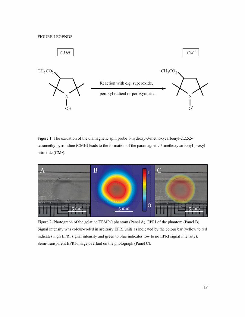
Figure 1. The oxidation of the diamagnetic spin probe 1-hydroxy-3-methoxycarbonyl-2,2,5,5-
tetramethylpyrrolidine (CMH) leads to the formation of the paramagnetic 3-methoxycarbonyl-proxyl
nitroxide (CM•).
Figure 2. Photograph of the gelatine/TEMPO phantom (Panel A). EPRI of the phantom (Panel B).
Signal intensity was colour-coded in arbitrary EPRI units as indicated by the colour bar (yellow to red
indicates high EPRI signal intensity and green to blue indicates low to no EPRI signal intensity).
Semi-transparent EPRI-image overlaid on the photograph (Panel C).
18
Figure 3. 2D plot of the EPR spectra after deconvolution as a function of gradient angle in the ZY
plane (to the left in the figure). Signal intensity was colour-coded in arbitrary EPR units as indicated
by the colour bar (yellow to red has more positive amplitude and green to blue is indicative of less
amplitude). EPR spectra for two particular gradient angles (θ = 4° and θ = 90°) (right).
Figure 4. EPRI signal intensity along on line in the EPR image as a function of the z-axis (along B0)
of the 1 mM TEMPO /gelatine phantom shown in Figure 2A. Panel A shows EPRI signal intensity for
19
three different Gaussian filters for spectral deconvolution. Panel B shows EPRI signal intensity for
three different Shepp-Logan filters used in the filtered back-projection.
Figure 5. EPR spectra after deconvolution for one section of one of the studied atherosclerotic plaques
(plaque 1, section 1) (left). EPR spectra for two particular gradient angles (θ = 4° and θ = 90°) are
shown to the right.

20
Figure 6. Photograph of the section (plaque 1, section 1) used to obtain the data in shown in Figure 5
located on the EPR tissue cell immediately after cryosection, incubation with spin trap and after
covering with Parafilm (panel A). Panel B: EPR image obtained after reconstruction of the data
shown in figure 5. Note that most part of the plaque gives some EPRI intensity but certain areas
shows high concentration of spin probe signal. Panel C shows the areas with highest EPRI intensity
fused onto the photograph. Panel D shows the histology of an adjacent slice with the high signalling
areas superimposed as dashed outlines. The arrow points at the thrombus formation protruding into
the lumen from the wall. L; lumen, C; lipid core. Scale bar correspond to 5 mm. The high
magnification insert shows aggregations of foamy macrophages taken from the upper high signalling
area.

21
Figure 7. EPRI similar to Figure 6 but obtained from a different section from a different
atherosclerotic plaque (plaque 2, section 1). Panel A shows a photograph of the section located on the
EPR tissue cell immediately after cryosection, incubation with spin trap and after covering with
Parafilm. Panel B shows the EPRI image obtained after reconstruction and panel C shows the areas
with highest EPRI intensity fused onto the photograph. Panel D shows the immunohistochemistry of
an adjacent slice of which the slice where the EPRI was carried out.

22
Figure 8. The areas with highest EPRI intensity fused onto the photographs of the remaining four
sections. Plaque 1, section 2 (Panel A), plaque 3, section 1 (Panel B), plaque 2, section 2 (Panel C)
and plaque 3, section 2 (Panel D).

23
Figure 9. The figure shows the projections (max values) along z axis (along B0) from the final
reconstructed EPR images shown in Figure 2 for the gelatine/TEMPO phantom, and from the two
sections from two different atherosclerotic plaques shown in Figure 6 (plaque 1, section 1) and Figure
7 (plaque 2, section 1).

24
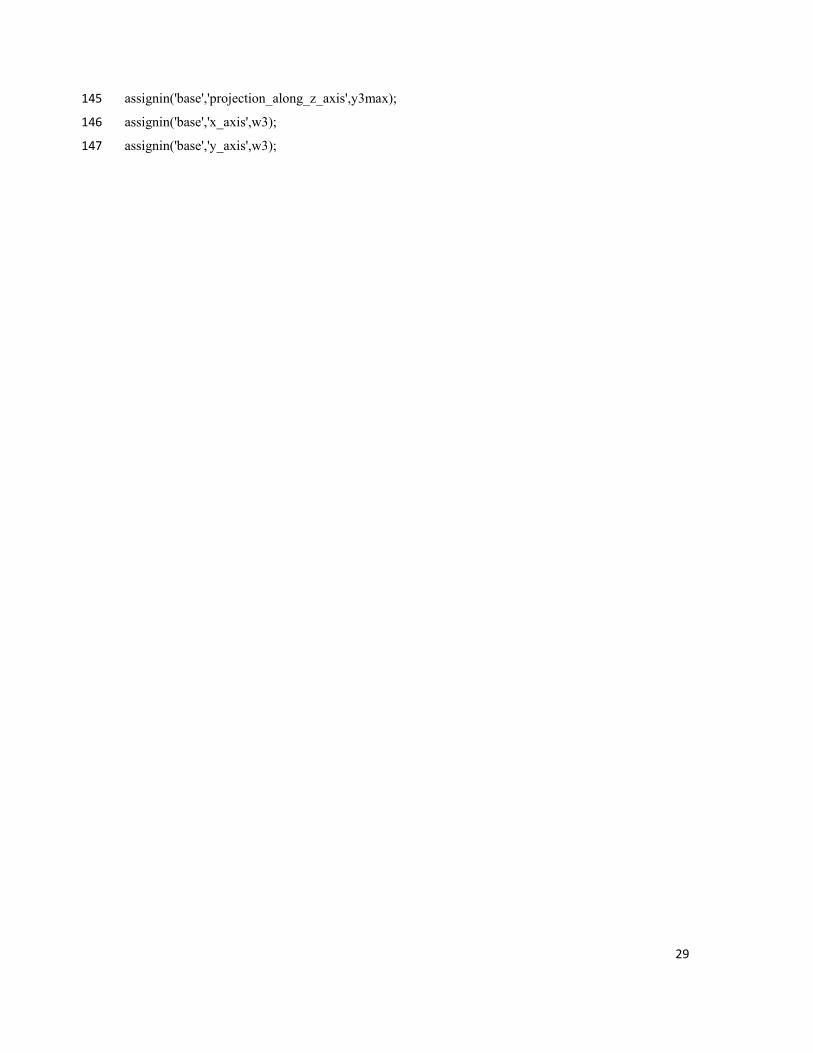
SUPPORTING INFORMATION
Matlab m-file for import of Bruker raw-data, deconvolution, back projection and image
reconstruction.

25
function [] = EPRI_tissue_cell 1
%File which reconstructs 2D EPRI from X Band EPR. 2
% 3
%function [] = EPRI_tissue_cell 4
% 5
% Håkan Gustafsson, December 2012. 6
7
clear all 8
close all 9
10
%Import of files. 11
file_name_1 = (input('Filename for measurement with gradient: ','s')); 12
[q1a,q1b,q1c] = eprload(file_name_1); 13
file_name_2 = (input('Filename for measurement without gradient: ','s')); 14
[~, w2] = eprload(file_name_2); 15
16
r1(:,1)=q1a{1,1}./10; % Magnetic field. 17
r2(:,1)=q1a{1,2}; % Gradient angles. 18
r3=rot90(q1b); 19
20
%Base line subtraction. 21
[raws ~]=size(r3); 22
for r4=1:raws 23
k=(r3(r4,end)-r3(r4,1))/(r1(end,1)-r1(1,1)); %y=kx+m 24
m=r3(r4,1)-r1(1,1)*k; 25
straight(r4,:)=k*r1(:,1)+m; 26
end 27
r5=r3-straight; 28
29
figure, 30
subplot(2,2,[1 2]), contourf(r1(1:2:end),r2(1:2:end),r5(1:2:end,1:2:end),100,'LineStyle','none') 31
c=colorbar; 32
ylabel(c,'EPR signal intensity (arbitrary units)'); 33
colormap jet 34
xlabel('B_0 (mT)'); 35
ylabel('Gradient angle \theta ( ^{o} \theta)'); 36
26
title('Raw data') 37
subplot(2,2,3), plot(r1(:),r5(1,:),'k'); 38
xlabel('B_0 (mT)'); 39
title(['Angle \theta = ',num2str(r2(1)),' ^{o}']); 40
r6=round(raws/2); 41
subplot(2,2,4), plot(r1(:),r5(r6,:),'k'); 42
xlabel('B_0 (mT)'); 43
title(['Angle \theta = ',num2str(r2(r6)),' ^{o}']); 44
45
%Deconvolution 46
t1=r5; 47
t2=w2; 48
t3='y'; 49
fwhm=300; %Default 50
filter=0.1; %Default 51
t8=1; 52
while t3=='y' 53
points = length(t1(1,:)); 54
if t8 >= 2 55
fwhm=input('Choose fwhm for Gaussian filter used in deconvolution (default fwhm = 300) -> '); 56
filter=input('Choose filter for back-projection between 0 and 1 (default filter = 0.1) -> '); 57
end 58
for t4=1:raws 59
x_in_fourier_domain = linspace(0,1024,points); 60
x0 = 0; 61
h = gaussian(x_in_fourier_domain, x0, fwhm); 62
h = h'/max(h); 63
t5=transpose(t1(t4,:)); 64
t6 = ifft((fft(t5).*h)./(fft(t2))); 65
t6 = rot90(rot90(ifftshift(t6))); 66
t7(t4,:)=real(t6); 67
end 68
figure, 69
subplot(2,2,[2 1]),contourf(r1(1:2:end),r2(1:2:end),t7(1:2:end,1:2:end),100,'LineStyle','none') 70
d=colorbar; 71
ylabel(d,'Signal intensity after deconvolution (arbitrary units)'); 72

27
colormap jet 73
xlabel('B_0 (mT)'); 74
ylabel('Gradient angle \theta ( ^{o} \theta )'); 75
title(['After deconvolution (Gaussian filter with fwhm = ',num2str(fwhm),') .']) 76
subplot(2,2,3), plot(r1(:),t7(1,:),'k'); 77
title(['Angle \theta = ',num2str(r2(1)),' ^{o}']); 78
xlabel('B_0 (mT)'); 79
t4=round(raws/2); 80
subplot(2,2,4), plot(r1(:),t7(t4,:),'k'); 81
title(['Angle \theta = ',num2str(r2(t4)),' ^{o}']); 82
xlabel('B_0 (mT)'); 83
84
%Axis in mm scale 85
r1(:,1)=q1a{1,1}; 86
q8=q1c; 87
q7=q8.XMIN; 88
q9=q8.XWID; 89
q10=q7+q9/2; 90
q11=q8.GRAD; 91
q12=q1a{1,1}-q10; 92
q13(:,1)=10*q12/q11; 93
94
t9=rot90(rot90(t7')); 95
t10 = iradon(t9,r2,'linear','Shepp-Logan',filter); 96
w_min=q13(1); 97
w_max=q13(end); 98
w2=size(t10); 99
w3=[w_min:(abs(w_max)+abs(w_min))/(w2(1,1)-1):w_max]; 100
figure, contourf(w3,-1*w3,t10,50,'LineStyle','none'); 101
colormap gray 102
xlabel('mm'); 103
ylabel('mm'); 104
axis square 105
grid on 106
e=colorbar; 107
ylabel(e,'EPRI signal intensity (arbitrary units)'); 108

28
colormap jet 109
title(['EPRI of sample ',num2str(file_name_1),' after deconvolution (Gaussian filter fwhm = 110
',num2str(fwhm), ') and filtered backprojection (Shepp-Logan filter = ',num2str(filter),' ).']) 111
t3 = input('Try other settings for deconvolution filter and/or filter for backprojection? Yes (y) or no 112
(n)? ','s'); 113
t8=t8+1; 114
end 115
116
assignin('base','signal',t10); 117
disp('To plot image write e.g. imagesc(x_axis,y_axis,signal).') 118
119
%Projection along each axis. 120
121
for y1 = 1:w2 122
y2max(y1)=max(t10(y1,1:end)); 123
end 124
125
for y1 = 1:w2 126
y3max(y1)=max(t10(1:end,y1)); 127
end 128
129
figure,plot(w3,y2max,'k'); 130
grid on 131
title('Projection (max values) along y axis (sample tube axis).') 132
axis square 133
xlabel('y axis (mm) (along sample tube)'); 134
ylabel('EPR signal intensity (arbitrary units)'); 135
legend('max value along axis') 136
figure,plot(w3,y3max,'k'); 137
grid on 138
title('Projection (max values) along z axis (sample B_0).') 139
axis square 140
xlabel('z axis (mm) (along B_0)'); 141
ylabel('EPR signal intensity (arbitrary units)'); 142
legend('max value along axis') 143
assignin('base','projection_along_y_axis',y2max); 144
29
assignin('base','projection_along_z_axis',y3max); 145
assignin('base','x_axis',w3); 146
assignin('base','y_axis',w3); 147