visualisations for comparing self-organising mapsandi/download/thesis/bau_thesis07.pdf ·...

M A S T E R A R B E I T

Visualisations for ComparingSelf-organising Maps

ausgefuhrt am Institut fur

Softwaretechnik und Interaktive Systeme

der Technischen Universitat Wien

unter der Anleitung vonao.Univ.Prof. Dipl.-Ing. Dr.techn. Andreas Rauber

durch

Doris BaumMatrikelnummer: 0426038

Friedrich-Ruckert-Weg 1090547 Stein

Deutschland

Wien, am 16. Marz 2007

2

Acknowledgements

I’d like to thank Andreas Rauber for being the best supervisor I could have wishedfor, always encouraging, always envisioning new possibilities, and always asking for

one more check-box in the GUI.I thank Thomas Lidy, Rudolf Mayer, Georg Polzlbauer, Robert Neumayer, and

Angela Roiger for indispensable help, encouragement, and lunches.

I thank my parents for their unquestioning support,both financial and emotional,

and all my friends for their patience and understanding,especially Florian Ruckeisen and Judith Oliva.

3

Zusammenfassung

Self-organising Maps (SOMs) sind ein sehr nutzliches Werkzeug um große Daten-sammlungen zu untersuchen und zu analysieren: Sie projizieren hochdimensionaleDaten in einen niedrigdimensionalen Raum, so dass die Daten leichter von Menschenanalysiert werden konnen als in ihrer ursprunglichen Form. Zum Zweck der Analyseexistieren viele Visualisierungen, die verschiedene Aspekte und Eigenschaften derSOMs und der Daten darstellen. Es gibt allerdings sehr wenige Visualisierungen umzwei oder mehr SOMs direkt mit einander zu vergleichen. Um dies zu beheben stelltdiese Arbeit drei Visualisierungen vor, die SOMs vergleichen, die auf dem gleichenDatenset mit unterschiedlichen Parametern trainiert wurden. Damit soll heraus-gefunden werden, wo die Daten jeweils auf den Karten zu liegen kommen und dieStabilitat und Qualitat der Projektionen eingeschatzt werden.

Abstract

Self-organising Maps (SOMs) are a very useful method for exploring and analysinglarge data collections: They project high-dimensional data into a low-dimensionaloutput space so that it is easier to analyse for humans than the original data. For thepurpose of analysis, plenty of visualisations exist which display different aspects andproperties of the maps and the data. There are, however, very few visualisations fordirectly comparing two or more SOMs with each other. This work tries to rectify thatby introducing three visualisations to compare SOMs trained on the same datasetwith different parameters, to find out where the data comes to lie on each map andassess the stability and quality of the projections.

Contents

1 Introduction 6

2 Self-organising Maps (SOMs) 7

2.1 Introduction . . . . . . . . . . . . . . . . . . . . . . . . . . . . . . . . 72.2 SOM Visualisations . . . . . . . . . . . . . . . . . . . . . . . . . . . . 92.3 Cluster Analysis on SOMs . . . . . . . . . . . . . . . . . . . . . . . . 112.4 Measuring the Quality of a SOM’s Projection . . . . . . . . . . . . . 122.5 Comparing Multiple SOMs . . . . . . . . . . . . . . . . . . . . . . . 132.6 Summary . . . . . . . . . . . . . . . . . . . . . . . . . . . . . . . . . 13

3 Visualisations 15

3.1 Data Shifts Visualisation . . . . . . . . . . . . . . . . . . . . . . . . . 153.1.1 Definition of the Neighbourhood . . . . . . . . . . . . . . . . 163.1.2 Data Shift Definition and Types . . . . . . . . . . . . . . . . 173.1.3 Mathematical Formalisation . . . . . . . . . . . . . . . . . . . 203.1.4 Example . . . . . . . . . . . . . . . . . . . . . . . . . . . . . . 21

3.2 Cluster Shifts Visualisation . . . . . . . . . . . . . . . . . . . . . . . 223.2.1 Cluster Mapping . . . . . . . . . . . . . . . . . . . . . . . . . 223.2.2 Example . . . . . . . . . . . . . . . . . . . . . . . . . . . . . . 24

3.3 Comparison Visualisations for Multiple SOMs . . . . . . . . . . . . . 253.3.1 Computing the Comparison Visualisations . . . . . . . . . . . 253.3.2 Mathematical Summary of the Computation . . . . . . . . . 273.3.3 Calculation of the Distance Matrix . . . . . . . . . . . . . . . 273.3.4 Example . . . . . . . . . . . . . . . . . . . . . . . . . . . . . . 29

3.4 Summary . . . . . . . . . . . . . . . . . . . . . . . . . . . . . . . . . 30

4 Datasets Used in the Experiments 31

4.1 Equidistant Gaussian Clusters . . . . . . . . . . . . . . . . . . . . . . 314.2 Intertwined Rings Dataset . . . . . . . . . . . . . . . . . . . . . . . . 334.3 Complex Artificial Cluster Dataset . . . . . . . . . . . . . . . . . . . 344.4 Iris Data Set . . . . . . . . . . . . . . . . . . . . . . . . . . . . . . . 354.5 Summary . . . . . . . . . . . . . . . . . . . . . . . . . . . . . . . . . 35

4

CONTENTS 5

5 Experiments 36

5.1 Data Shifts Visualisation on the Complex Artificial Cluster Dataset 365.1.1 Checking Results with Cluster Shifts Visualisation and Com-

parison Visualisation . . . . . . . . . . . . . . . . . . . . . . . 415.2 Cluster Shifts Visualisation on the Equidistant Gaussian Cluster Data-

sets . . . . . . . . . . . . . . . . . . . . . . . . . . . . . . . . . . . . . 435.2.1 Checking Results with Data Shifts Visualisation and Compar-

ison Visualisation . . . . . . . . . . . . . . . . . . . . . . . . . 465.3 Comparison Visualisation on the Intertwined Rings Dataset . . . . . 48

5.3.1 Checking Results with Data Shifts Visualisation and ClusterShifts Visualisation . . . . . . . . . . . . . . . . . . . . . . . . 52

5.4 Assessing SOM Quality on Equidistant Gaussian Cluster Dataset “5” 545.4.1 Data Shifts Visualisation . . . . . . . . . . . . . . . . . . . . 545.4.2 Cluster Shifts Visualisation . . . . . . . . . . . . . . . . . . . 565.4.3 Comparison Visualisation . . . . . . . . . . . . . . . . . . . . 56

5.5 Test on Real-life Data: Iris Dataset . . . . . . . . . . . . . . . . . . . 595.5.1 Data Shifts Visualisation . . . . . . . . . . . . . . . . . . . . 595.5.2 Cluster Shifts Visualisation . . . . . . . . . . . . . . . . . . . 625.5.3 Comparison Visualisation . . . . . . . . . . . . . . . . . . . . 64

5.6 Summary . . . . . . . . . . . . . . . . . . . . . . . . . . . . . . . . . 65

6 Future Work 66

7 Conclusion 68

A List of Tables 69

B List of Figures 72

C Bibliography 74

Chapter 1

Introduction

Self-organising Maps (SOMs) are a very useful method for data exploration: Theyproject high-dimensional data onto a low-dimensional output space, a two-dimensionalgrid, so that it can be more easily analysed by humans than the original data. Forthe purpose of analysis, plenty of visualisations exist which display different aspectsand properties of the maps and the data. There are, however, very few approachesfor directly comparing two or more SOMs with each other. This work tries to rec-tify that by introducing three visualisations to compare SOMs trained on the samedataset with different parameters. Two of them display where the data comes tolie on each map, showing the differences and similarities of two maps, while thethird compares “arbitrarily many” SOMs with each other (where the number is ofcourse limited by computing power). All three methods can be used to asses thestability and quality of the projection the SOM performs, as well as the influence ofthe parameters used. The visualisations were implemented in an existing frameworkfor SOM training and visualisation, the SOMViewer project, and experiments onsynthetic and real-world datasets were conducted. The tests lead to the conclusionthat the proposed visualisations can indeed be useful in data exploration.Chapter 2 gives an introduction to Self-organising Maps and shortly describes re-lated work: SOM visualisations, cluster analysis on SOMs, quality measures, andcomparing multiple SOMs. Chapter 3 explains the visualisations introduced in thiswork, while Chapter 4 describes the datasets used in the experiments. The actualexperiments are detailed in Chapter 5, a few possible improvements of the visuali-sations are proposed in Chapter 6, and Chapter 7 closes this work.

6

Chapter 2

Self-organising Maps (SOMs)

2.1 Introduction

Self-organising Maps (SOMs) were introduced by Teuvo Kohonen [5], [6], thereforesometimes also called Kohonen maps. They are a type of artificial neural networkand an unsupervised machine learning method (see, for example, [2] for a detailedexplanation of these terms).SOMs serve as an instrument for topology-preserving, low-dimensional visualisationof high-dimensional data, similar to Multidimensional Scaling [7]. That is, theyproject data from a high-dimensional input space onto a low-dimensional (usually2-dimensional) output space, trying to preserve the closeness relations of the datasamples. Visualisations of the resulting output space can be very useful in dataexploration to get an impression of the properties of the data.SOMs consist of artificial neurons placed in a low-dimensional (usually 2-dimensionalbecause this is easiest to visualise) grid with a rectangular or hexagonal lattice.Throughout the experiments in this work, a rectangular grid is used. Throughtheir position on the grid, the neurons’ distance relation is defined like on a map;for example, adjacent units on the grid are considered “close”, whereas units inopposing corners of the grid are considered “far apart”.The units are represented by prototype vectors mk in the input space. Prior to thetraining phase, the units’ prototype vectors are initialised to random values in manySOM implementations. To shorten the training phase, the prototype vectors mayalso be initialised to non-random values constructed from the data.During the training phase, a simple training step is repeated many times to make themap of prototype vectors fit the input data closely, so as to give a good projectionof the data:

1. Select a data sample x(t) from the input data, for example randomly.

2. Find the prototype vector c closest to the data sample. The unit it representsis called the Best Matching Unit (BMU) for that data sample.

7

CHAPTER 2. SELF-ORGANISING MAPS (SOMS) 8

Figure 2.1: A SOM’s prototype vec-tors in the input space before train-ing.

Figure 2.2: A SOM’s prototype vec-tors in the input space after training.

3. Move all prototype vectors towards the data sample, proportionally to theircloseness to the BMU. That is, if a unit is close to the BMU, move its prototypevector more than if the unit is far away from the BMU. The rule for the newposition of the prototype vectors is

mk(t + 1) = mk(t) + α(t)hck(t)(x(t)−mk(t)) (2.1)

where mk(t + 1) is the new position of the prototype vector (at step t + 1),mk(t) is the old position (at step t), x(t) is the selected data sample, a(t) isthe learning rate and hck(t) is a neighbourhood kernel around BMU c. Theneighbourhood kernel defines the measure for the units’ “closeness” to theBMU; often, a Gaussian kernel depending on the grid lattice distance to theBMU is used.

Both learning rate and neighbourhood kernel decrease monotonically withtime, so that learning starts quick and on a global scale and gradually be-comes slower and more local. The SOMViewer software used in this work togenerate and analyse SOMs uses negative exponential functions to determinethe current learning rate and size of neighbourhood.

Through the training, the SOM folds onto the data like a flexible net, giving a2-dimensional projection of the data on the grid, trying to preserve topologicalproperties of the data. Because of the neighbourhood kernel, similar prototypevectors end up in each other’s neighbourhood, so similar data vectors are mappedonto units close to each other on the grid. Thus, similarity is mirrored by closenessin a SOM.Figures 2.1 and 2.2 show a SOM’s prototype vectors and their grid in the input dataspace (the black dots and lines), together with the input data (the red, green, andblue dots, each colour marks a class). Both figures were produced with the Matlab


Figure 2.3: Example of a U-matrix. Figure 2.4: Example of a hit his-togram.

SOM Toolbox1. Figure 2.1 shows the SOM randomly initialised but yet untrained.Figure 2.2 shows the same SOM after training – with the SOM adjusted to the shapeof the data.

2.2 SOM Visualisations

There are numerous visualisation methods for SOMs, the basic and most frequentlyused ones summed up in [17].

Maybe the most prominent one is the U-matrix [14] which shows each prototypevector’s/unit’s euclidean distance to its neighbours in shades of grey, different huesof colour, by shape, or in some other way. An example for a U-matrix is depicted inFigure 2.3; it shows a SOM made with the SOMViewer software [3] from dataset “6”described in Section 4.1 (page 31). The dataset contains three equidistant clustersof samples taken from Gaussian distributions. The SOM has 10 × 10 units drawnas squares with grey borders. High distance of prototype vectors is indicated bydark colour here – there clearly is a Y-shaped black “rift” through the SOM, whichseparates three light areas. Looking at the data (see Figure 4.1, page 32) revealsthat there are indeed three well-separated clusters. So the U-matrix can be used todiscern clusters and cluster borders during data exploration.

Another often used SOM visualisation is the data histograms or hit histogram. Itshows for each unit for how many data samples it was the Best Matching Unit –that is, how many hits of data vectors it scored. The number can be indicated bythe size of a marker on the unit’s grid cell, by colour, by 3-dimensional bar charts,or by simply printing the number into the unit’s cell. Figure 2.4 is an example for

1Matlab: http://www.mathworks.com/; SOM Toolbox: http://www.cis.hut.fi/projects/

somtoolbox/.

http://www.mathworks.com/

http://www.cis.hut.fi/projects/somtoolbox/

http://www.cis.hut.fi/projects/somtoolbox/


Figure 2.5: Example of a Smoothed Data Histogram with s = 10

a hit histogram; it was made from the same data and the same SOM as Figure 2.3.When comparing Figure 2.4 with Figure 2.3, one can see that the units in the blackrift in the U-matrix get very few hits or no hits at all in the hit histogram: they arethe Best Matching Unit for at most one or two data vectors. This is to be expectedalong the cluster borders because the input space is sparse with data there.

The Smoothed Data Histograms (SDH) visualisation [10] is an extension of the datahistogram visualisation. It is used to visualise clusters in the data on the SOM. Itestimates the probability density of the input data on the map by smoothing theresults of the normal data histogram. Instead of assigning a data vector only toa single Best Matching Unit, it is assigned to be a member of those s units whoseprototype vectors are closest to the data vector, i.e. the s Best Matching Units. Thedegree to which a data vector is a member of a unit is determined by the rank ofcloseness between the data vector and the unit’s prototype vector: The membershipdegree is highest for the closest unit, second highest for the second closest unit, andso on. The units of the SOM are coloured in the SDH according to the summedup membership degrees of the data vectors assigned to them. Figure 2.5 shows anexample of a Smoothed Data Histogram with s = 10; it was made from the samedata and the same SOM as the examples above. The clusters already detected inthe U-Matrix can also be seen in the SDH, there is a similar Y-shaped rift betweenthe clusters. The SDH additionally shows the density of the data on the map.

Although the SOM is an unsupervised learning method and is not trained on infor-mation about different classes of data, existing class information can be used in afurther visualisation. If there is information on which classes the input data vectorsbelong to, a class information visualisation can be drawn showing for each unit theclasses of the data vectors for which it is Best Matching Unit. Figure 2.6 showsan example of this: The data vectors are mapped onto their Best Matching Units,and the units get coloured markers according to the classes of their data vectors.The data and the SOM for Figure 2.6 are the same as for the other examples, andhere one can see the three different classes that make up the three clusters already


Figure 2.6: Example of class informa-tion visualisation.

Figure 2.7: Example of SOM cluster-ing.

detected in the other two visualisations. This, of course, is only possible if classinformation on the data is available, which is not necessarily the case when using aSOM for data exploration.

This section gives just a few examples of SOM visualisations but there are, of course,more. The main part of this work is dedicated to introducing three new variationsof SOM visualisations, which compare two or more SOMs with each other. Theyare explained in Chapter 3 and tested on data in Chapter 5.

2.3 Cluster Analysis on SOMs

Two of the visualisations introduced in Chapter 3 make use of the SOMViewer’scluster analysis methods described in [12]. Cluster analysis is used to find clusters/ groups / partitions in the data, which is an essential task in data mining andespecially data exploration, as is explained in depth for example in [13]. The clustersfound may represent the actual structure of the data or may be used to summarise orcompress it. The SOM algorithm can be seen as a kind of clustering algorithm itself –a unit’s prototype vector representing the cluster centre for the data vectors mappedon the unit. Thus an application of cluster analysis on a SOM is really an applicationof clustering on a compressed / reduced data set. This can reduce the computationalload needed for clustering greatly without losing too much on clustering accuracy,compared with cluster analysis on the original data, as is described in [18].Figure 2.7 shows a SOM class information visualisation (on the same data andSOM as the other figures) with cluster borders drawn in grey, which were obtainedby applying the Ward’s linkage clustering [20] and setting the number of clustersto 3. The borders overlap with the rift from Figure 2.3 and separate the classes inFigure 2.6, though not perfectly. As can be seen, cluster analysis can be used tofind a real structure underlying the data.


2.4 Measuring the Quality of a SOM’s Projection

A number of measures have been described for computing and comparing the qualityof a SOM’s projection (summed up in [11]), such as the Topographic Error, theTopographic Product [1], Trustworthiness and Neighbourhood Preservation [16],and special decompositions of the SOM Distortion Measure [19]. They all measure,in one way or another, how well the topology is preserved in the projection onto theSOM’s two-dimensional grid.

The Topographic Error is a simple measure: For all input data vectors, the nearestweight vector (Best Matching Unit) and the second-nearest weight vector (SecondBest Matching Unit) are computed. If they are not adjacent on the SOM-grid, thisis counted as a local error. For the global topographic error measure, the numberof local errors is summed up and divided by the overall number of data samples.

The Topographic Product [1] is based on two measures, P1 and P2, which indicatefor each unit whether its k nearest neighbour units coincide, regardless of their order.P1 assesses the input space, using the distances between the units’ prototype vectors,while P2 assesses the output space, using the euclidean grid distance between theunits. Both are combined into P3, which differs from 1 if there are violations ofneighbourhood and indicates whether the dimensionality of the output space is toolarge (P3 > 1) or too small (P3 < 1). The P3 values of the units on the map areaveraged to get a global measure P for the whole map, which also indicates whetherthe dimensionality of the map fits or is too large or too small.Because the Topographic Product uses distances of units and prototype vectors, theinput dataset is not needed for its computation.

The Neighbourhood Preservation [16] measure is similar to the Topographic Productin that it indicates how well the neighbourhood of the k nearest neighbours inthe input space is preserved in the projection onto the output space. A differenceis that it works with input data vectors instead of prototype vectors. However,the more important measure introduced in the paper is the Trustworthiness of theneighbourhoods in the output space. It assesses whether the k nearest neighbours ofa data vectors in the output space (the SOM-grid) are also close in the input space,thus giving an indication of the expressiveness and reliability of the output spaceview on the data.

The decomposition of the SOM Distortion measure introduced in [19] gives anotherpossibility to assess the quality of the projection. The SOM Distortion measure is alocal energy function of the SOM if the data set is discrete and the neighbourhoodkernel is fixed; the SOM training rule approximates the Distortion measure’s gra-dient. The decomposition introduced by Vesanto et al. splits the SOM Distortioninto three parts: local data variance, neighbourhood variance, and neighbourhood


bias. The local data variance gives the quantisation quality. The neighbourhoodvariance assesses the trustworthiness of the map topology, similar to the Trustwor-thiness measure from [16]. The neighbourhood bias links the other two and can beseen as the stress between them.

All of these measures can be used to compare SOMs and (to varying success) toselect the SOM that best fits the data. However, none of these measures comparestwo SOMs with each other or directly shows their differences.

2.5 Comparing Multiple SOMs

There is – to the current knowledge of this work’s author – only one approach tocomparing and visualising multiple SOMs trained on the same data: The conceptof Aligned Self-organising Maps, explained in [8] and [9]. It is used to train severalSOMs on the same data with slightly different feature extraction parameter settingsin order to explore the effects of these settings. The problem in comparing suchSOMs is that the data vectors and clusters will come to lie on different areas inthe individual SOMs due to different initialisation and parameters. To alleviate thisproblem, the Aligned SOMs are trained in such a way that each data vector canbe found in the same region on different maps. This requires an adaption of theSOM training algorithm: The SOMs are stacked on top of each other, so that eachSOM is a layer in the stack, and a distance measure between the layers is definedto control the smoothness of the transition between the SOMs. With this distancemeasure, a distance between units in different layers can be derived, which is usedin training in the same way that the distance between units in one SOM is used topreserve the topology of the data. That is, for the training step a data vector anda layer are selected, the Best Matching Unit in the layer is found, and the units inthe other layers are adapted according to their distance from the BMU. The unitswithin the layer are adapted according to the normal SOM training step. The resultis an Aligned SOM stack which “morphs” the first layer in the stack to the last.However, this method can’t be used on maps trained with the unmodified SOMalgorithm, or on maps with different sizes. The methods introduced in the nextchapter try to alleviate this.

2.6 Summary

In this chapter, the concept of the Self-organising Map (SOM) was explained briefly:The SOM is a method for topology-preserving projection of high-dimensional datainto a low-dimensional output space for the purpose of visualisation and data explo-ration. It is an artificial neural network whose neurons are represented by prototypevectors in the input space. The neurons are placed in a lattice which defines a dis-


tance relation between them. During the training phase, the prototype vectors areshifted to fit to the data, and each time a specific unit is shifted the units close toit on the lattice are shifted as well, relative to their closeness.Several visualisations for the SOM were shortly described: The U-Matrix, the datahistograms, the Smoothed Data Histograms (SDH), and the class information visu-alisation, which can all be used to gain information about the data and the SOM inquestion.Also, cluster analysis on SOMs was touched on as a method to detect existingclusters in the data or to summarise and compress it. The clusters found by clusteranalysis algorithms can also be visualised to gain insight into the structure of thedata.Several quality measures were described: the Topographic Error, the TopographicProduct, Trustworthiness and Neighbourhood Preservation and decompositions ofthe SOM Distortion Measure. They can all be used to assess and compare thequality of a SOM’s projection. However, they all measure the fit of a SOM to itsinput data, they don’t compare two SOMs directly.Finally, a method for comparing multiple SOMs trained on the same data was ex-plained: Aligned Self-organising Maps. It can be used to train and compare a stackof maps with slightly different feature parameter settings to explore the effects ofthese settings. However, the method can’t be used on maps trained with the originalSOM algorithm or maps with different sizes or number of training steps.All in all, this chapter gave an overview of the underlying concepts used in the nextchapters.

Chapter 3

Visualisations

This chapter introduces three new variations of SOM visualisations – the main dif-ference to other visualisations being that they are applied to two or more SOMs.They compare the SOMs and show were the data comes to lie on different SOMs,which indicates how stable the data projection is, and which properties of the SOMsare just artefacts of different parameter settings. Parameters comprise such settingsas the size of the SOM, the learning rate, the number of iterations, etc.The first visualisation, described in section 3.1, shows differences in the projection ofthe data vectors. The second one, explained in Section 3.2, compares cluster analysisdone on two SOMs. The third one, detailed in Section 3.3, compares “arbitrarilymany” SOMs (limited, of course, by the computing power needed for a comparisonof a large number of SOMs) and shows the average distances of data vectors in theSOMs’ projections.

3.1 Data Shifts Visualisation

The data shifts visualisation is applied to two SOMs trained on the same data withdifferent parameters. It can be used to detect differences between these SOMs: Itdisplays changes in the position of the data vectors relative to neighbouring datavectors on the SOMs. More precisely, the data shifts visualisation shows for aspecific data vector how many other vectors mapped onto neighbouring units in thefirst SOM are also mapped onto neighbouring units in the second SOM. This can beused to find out how stable the mapping is, how steadily a data vector is put intoa neighbourhood of similar vectors on different SOMs. Or more abstractly: Howmuch of the data topology on the map really is caused by attributes of the data, andhow much of it is simply an effect of different SOM parameters or initialisations.The moving data vectors are displayed as arrows drawn between the grid visuali-sations of the two maps – see Figure 3.1 to get a first impression of what it lookslike. The thickness of the arrows corresponds to the number of neighbours thatare the same in both maps, while the colour stands for the type of data shift (see

15

CHAPTER 3. VISUALISATIONS 16

Figure 3.1: Comparison of the position of data vectors on two different SOMs trainedon the same data with different parameters; The SOMs are visualised by the tworectangular grids, where each square depicts a SOM unit and each number is thenumber of data vectors mapped to that unit. The vectors on the unit marked inorange in the left SOM split up and move to two different units in the right SOM.The majority of vectors (3 of 4) moves to the unit marked with the green arrow,while one of the vectors moves to a different unit, marked with the red arrow (thisunit also has another vector mapped to it).

Section 3.1.2 for details).Of course, the visualisation inherently relies on the definition of the neighbourhoodused. Definition and adjustment of the neighbourhood in the data shifts visualisationare described in Section 3.1.1.To visualise the number of neighbours of a data vector that are the same in bothcompared SOMs, the notion of a “data shift” is defined together with three differenttypes of shifts, all described in Section 3.1.2.

3.1.1 Definition of the Neighbourhood

The distance function used in this visualisation is the SOM-grid distance in theoutput space. The distance between two data vectors is defined by the euclideangrid distance between the SOM units they are mapped to. For example, in Figure 3.1,the distance between the starting points of the arrows is 0 (as they lie on the sameunit in the left SOM), and the distance between the end points is 1 (as they lie onadjacent units in the right SOM). Based on this, the neighbourhood of a vector isdefined as the vectors lying within a certain radius around it. From this definition ofneighbourhood it follows (maybe a little counter-intuitively) that a vector is alwaysneighbour to itself. So each vector will have at least one neighbour – itself.Figure 3.2 illustrates which units around a selected centre unit are within the neigh-bourhood for a (very limited) number of radiuses. The vectors mapped to the unitswithin the radius naturally all are neighbours to the vectors on the centre unit. Theunits are marked with Roman numerals, and each radius comprises the units markedwith the corresponding numeral and all lesser numerals. A neighbourhood of radius0 only contains (vectors on) unit I; a neighbourhood with radius 1 contains unit I


Figure 3.2: Units that lie within a certain neighbourhood radius around a centre.

and all units marked with II; a radius of√

2 ≈ 1.41 holds units marked with I, II,and III (all bluish units); a radius of 2 holds units marked with IV and below; aradius of

√5 ≈ 2.24 holds all units with V and below (i.e. all coloured units), and

so on.

The neighbourhood radius can be separately adjusted for both SOMs; that is, whilethe neighbourhood radius in the first SOM (called source threshold) may be set to0, the radius in the second SOM (called target threshold) can be set to 5. This canbe useful if the map sizes of the SOMs differ: In the larger of the two SOMs, thereare more units for the data vectors to spread over, so vectors on the same unit in thesmaller SOM may scatter over adjacent units in the larger. If one is not interestedin this effect, the thresholds can be adjusted to compensate it.Additionally, there are two “modes” of the visualisation, “cumulative” and “non-cumulative”. The “non-cumulative” mode changes the neighbourhood radiuses fora part of the calculation of the data shift types (see next section for a detailed expla-nation of the types and the changes). In the “cumulative” mode the neighbourhoodradiuses remain unchanged.

3.1.2 Data Shift Definition and Types

The “data shifts” used to build this visualisation correspond to the data vectors’property to either stay with their neighbouring data vectors on both SOMs, or toleave their neighbours from the first SOM and move to a new area in the second SOM.They are represented by arrows of different colours and thickness, which are drawnbetween the grid visualisations of the two SOMs (see Figure 3.1 for an example).Different arrow types display where the majority of vectors from a neighbourhoodon the first SOM moved to on the second SOM, and where the separating outlierscome to lie.During the calculation process of the visualisation, a shift is produced for each datavector on the maps, unnecessary doublets are discarded later on. A data shift hasseveral attributes:


Count / Thickness: The data shift’s “neighbour count” or just “count”, which isrepresented as the arrow’s thickness.

This is the number of data vectors that are both in the “old” neighbourhoodand in the “new” neighbourhood of the data vector in question. This count isalways at least one because each vector is neighbour to itself.

If the “non-cumulative” mode is used, the neighbourhood radiuses are changed.They are set to 0 for determining the count (but not for the adjacent shifts,see below). This effectively means that only vectors that move together froma certain unit on the first SOM to the same unit on the second SOM, areconsidered neighbours and increase the count. If the “cumulative” mode isused, the neighbourhood radiuses remain unchanged, and vectors within theradius also count as neighbours.

That is, if both neighbourhood radiuses are 5 and the “non-cumulative” modeis used only the data vectors mapped onto the same unit with the data vectorin question are regarded as neighbours. However, if the “cumulative” mode isused, all data vectors mapped to units with a euclidean distance of 5 or lessfrom the specified data vector’s Best Matching Unit are regarded as neigh-bours.

If the thresholds that determine the data shift type (see below) are given asabsolute values, the neighbour count is visualised by the thickness of the arrowthat represents the data shift.

Percentage / Thickness: The percentage of old neighbours which are also newneighbours. This is just the count divided by the total number of neighbours inthe old neighbourhood. The percentage may alternatively be used to determinethe arrow’s thickness.

If the thresholds that determine the data shift type (see below) are given aspercent values, the percentage is visualised by the thickness of the arrow thatrepresents the data shift.

So, how the thickness of the arrow is calculated depends on whether the thresh-olds are absolute values or percentages.

Coordinates: The coordinates of the shift. That is, the SOM grid coordinates ofthe two units the vector in question is mapped to.

These positions are, of course, visualised as the start and end points of thearrow representing the data shift.

Type / Colour: The shift type, one of “stable”, “adjacent”, or “outlier”, whichdetermines the colour of the arrow. The type is determined by measuring theneighbour count or percentage against two thresholds which can be adjusted


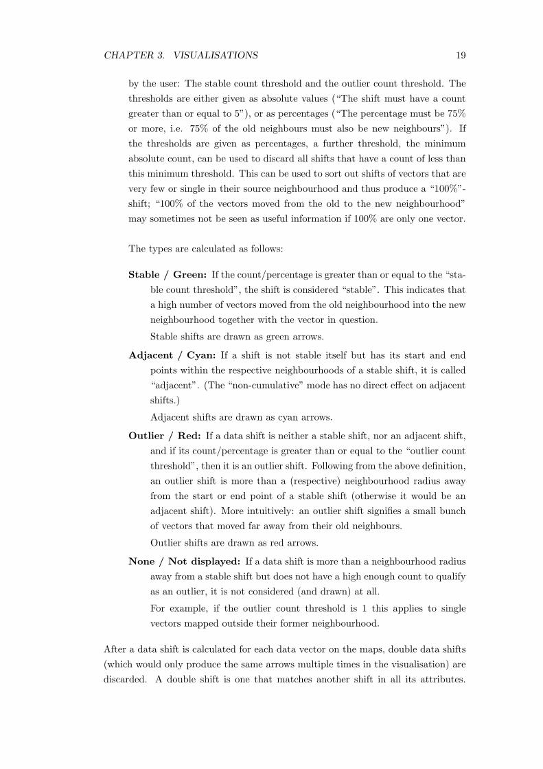
by the user: The stable count threshold and the outlier count threshold. Thethresholds are either given as absolute values (“The shift must have a countgreater than or equal to 5”), or as percentages (“The percentage must be 75%or more, i.e. 75% of the old neighbours must also be new neighbours”). Ifthe thresholds are given as percentages, a further threshold, the minimumabsolute count, can be used to discard all shifts that have a count of less thanthis minimum threshold. This can be used to sort out shifts of vectors that arevery few or single in their source neighbourhood and thus produce a “100%”-shift; “100% of the vectors moved from the old to the new neighbourhood”may sometimes not be seen as useful information if 100% are only one vector.

The types are calculated as follows:

Stable / Green: If the count/percentage is greater than or equal to the “sta-ble count threshold”, the shift is considered “stable”. This indicates thata high number of vectors moved from the old neighbourhood into the newneighbourhood together with the vector in question.

Stable shifts are drawn as green arrows.

Adjacent / Cyan: If a shift is not stable itself but has its start and endpoints within the respective neighbourhoods of a stable shift, it is called“adjacent”. (The “non-cumulative” mode has no direct effect on adjacentshifts.)

Adjacent shifts are drawn as cyan arrows.

Outlier / Red: If a data shift is neither a stable shift, nor an adjacent shift,and if its count/percentage is greater than or equal to the “outlier countthreshold”, then it is an outlier shift. Following from the above definition,an outlier shift is more than a (respective) neighbourhood radius awayfrom the start or end point of a stable shift (otherwise it would be anadjacent shift). More intuitively: an outlier shift signifies a small bunchof vectors that moved far away from their old neighbours.

Outlier shifts are drawn as red arrows.

None / Not displayed: If a data shift is more than a neighbourhood radiusaway from a stable shift but does not have a high enough count to qualifyas an outlier, it is not considered (and drawn) at all.

For example, if the outlier count threshold is 1 this applies to singlevectors mapped outside their former neighbourhood.

After a data shift is calculated for each data vector on the maps, double data shifts(which would only produce the same arrows multiple times in the visualisation) arediscarded. A double shift is one that matches another shift in all its attributes.


Double shifts are quite easy to find, because if the shifts coordinates match (theshifts go from the same unit to the same unit), all other attributes will match aswell. The count and percentage must be the same because the number of neighboursis the same, and the type must be the same because the types’ conditions mutuallyexclude each other and cannot be fulfilled for more than one type at the same time.

3.1.3 Mathematical Formalisation

The data shifts and their types can be mathematically formalised as follows:Let r1 and r2 be the radiuses of the source and target neighbourhoods (source andtarget threshold), and let d1 and d2 be the distance functions in the output spaceof the source and target SOM. Let cs be the stable count threshold and co be theoutlier count threshold. xi is the data vector in question. Then xi’s source andtarget neighbourhoods U1i and U2i contain other data vectors as follows:

U1i = {xj |d1(xj , xi) ≤ r1} (3.1)

U2i = {xj |d2(xj , xi) ≤ r2} (3.2)

The set of neighbours that are in both neighbourhoods, Si can easily be found, aswell as the set of vectors that are neighbours in the first SOM but not in the second,Oi:

Si = U1i ∩ U2i (3.3)

Oi = U1i \ U2i (3.4)

If the count thresholds are given as absolute values, vector xi’s data shift is stable if|Si| ≥ cs. On the other hand, if the count thresholds are given as percentages, thedata shift is a stable shift if |Si|

|U1i| ≥ cs.

If the data shift is not a stable shift, it is an adjacent shift if there is another datavector xs whose data shift is stable and

d1(xi, xs) ≤ r1 ∧ d2(xi, xs) ≤ r2. (3.5)

Finally, if the shift is neither stable nor adjacent, it is an outlier shift if |Oi| ≥ co

and the count thresholds are given as absolute values. In case the count thresholdsare given as percentages, the shift is an outlier if |Oi|

|U1i| ≥ co.


Figure 3.3: Part of a data shifts visualisation focusing on the vectors on the unitmarked with the blue box. The source and target thresholds (neighbourhood ra-diuses) are 1, the “non-cumulative” mode is active, and the stable and outlier countthresholds are 2 and 1 respectively. The circles represent the neighbourhood radiusesfor determining the neighbour count (green) and the adjacent shifts (cyan) of thevectors in question.

3.1.4 Example

The definitions above may seem quite abstract, but what does the visualisation looklike and what does it mean? See Figure 3.3 for an example of different data shifttypes explained on two very small maps.The parameters for this visualisation are a source threshold (neighbourhood radiuson the left map) of 1 and a target threshold (neighbourhood radius on the right map)of 1. The “non-cumulative” mode is active, so the neighbourhood radiuses are setto 0 for determining the counts; therefore only vectors that go from the same unitto the same unit count towards the neighbour count. The stable count threshold is2, while the outlier count threshold is 1.The focus is on the three vectors on the unit marked with the blue box and theirneighbours. Two of the three vectors move to the unit in the top right corner ofthe right map, one moves away from the other two (to the unit with the third greencircle). The green circles mark the neighbourhoods used for determining the countof the three data shifts. So the vectors that move to the top right corner each havetwo neighbours that move with them (one of the neighbours being themselves), theircount is 2. The other vector has only one neighbour that moves with it – itself. Thisyields two stable shifts and one outlier shift. The two stable shifts would produceexactly the same arrow, so one of them is discarded and the remaining one is shownas the green arrow.As we have a stable shift now, we can check whether it has any adjacent shifts thatmove from its source neighbourhood to its target neighbourhood (but don’t have ahigh enough count to be stable). The neighbourhood radiuses are both 1, the cyancircles mark the relevant areas on the SOM. If there is a vector that moves from


the left cyan circle to the right cyan circle, it yields an adjacent shift. There is oneindeed, which moves from the bottom right corner of the left map to the top leftcorner of the right map, marked with the cyan arrow. All the other vectors havea count of only 1 and don’t start and end in the cyan circles, so they are outliers,drawn as red arrows.

3.2 Cluster Shifts Visualisation

The cluster shifts visualisation is conceptionally similar to the data shifts visual-isation introduced in section 3.1. However, it works on clusters instead of unitsor neighbourhoods. It operates on two SOMs, which it compares to find out howsimilar the results of clustering on both maps are.Using the clustering functionality of the SOMViewer [12], the SOMs are clusteredwith Ward’s linkage [20], and the same (user-adjustable) number of clusters is ex-tracted from the cluster trees for both SOMs. The clusters of both maps are identi-fied with each other, and these mappings are then visualised. In the style of the datashifts visualisation, blue arrows are used to indicate which cluster in the first SOM ismapped onto which cluster in the second SOM. Additionally, the data vectors whichmove from a cluster in the first SOM to the assigned cluster in the second SOM isconsidered “stable” shift, and a vector which moves to another cluster is consideredan “outlier”. Again, these are drawn as green and red arrows. Figure 3.4 showsan example of a cluster shift visualisation of two SOMs which were both trained onsynthetic data. The data was generated to contain two slightly overlapping Gaussianclusters. The number of clusters to find was set to two by the user.

3.2.1 Cluster Mapping

Obviously, a mapping from the clusters in the first SOM onto the clusters in thesecond SOM must be found for this visualisation to work. The method used isdescribed below, although other methods are conceivable – for ideas see Chapter 6.

The mapping used in the data shifts visualisation is determined from the agreementof data vectors in the clusters of the first and second SOM: The more data vectorsfrom cluster Ai in the first SOM are mapped into cluster Bi in the second SOM, thehigher the confidence pji that cluster Ai corresponds to cluster Bj .To put it mathematically: Let set Mij contain all data vectors x which are in Ai

and in Bj . To compute the confidence pij that Ai should be mapped onto Bj , thecardinality of Mij is divided by the cardinality of Ai.

Mij = {x|x ∈ Ai ∧ x ∈ Bj} (3.6)


Figure 3.4: A cluster shifts visualisation, showing two SOMs clustered into twoclusters each. The cluster borders are drawn as grey lines. The blue arrows indicatewhich cluster has been mapped onto which, whereas the green arrows depict the datavectors that stayed within clusters mapped onto each other, and the red arrows showdata vectors not mapped into corresponding clusters.

pij =| Mij || Ai |

(3.7)

To compute all confidence values, a table with entries for all possible mappings isprepared and initialised to 0s. Then the list of data vectors is traversed and thetable entries are updated: When a vector moved from cluster Ai to cluster Bj , thetable entry for Ai 7→ Bj is increased by one. After that, the table entries are dividedby the number of data vectors in cluster Ai. This yields the percentage of datavectors from cluster Ai that moved to cluster Bj , the measure for confidence, for allpossible mappings.From the table of confidences, the final mapping is derived: The entries are sortedaccording to confidence, and the mapping Ai 7→ Bj from the highest entry is takenas the first definite cluster assignment. Then all table entries concerning either Ai

or Bj are excluded from the further search, and the next highest entry is picked asthe next definite assignment. This step is repeated until all clusters in both SOMshave been assigned.When the mapping is determined, the visualisation can easily be drawn. The clustermappings are indicated by blue arrows, whose thickness corresponds to the confi-dence of the assignment. The stable (green) shifts are shifts from a cluster in thefirst SOM to the assigned cluster in the second SOM. The outlier (red) shifts areshifts into other clusters.


Cluster in 1st SOM Cluster in 2nd SOM Confidence3 2 90%2 2 90%0 3 85%1 0 54%1 1 46%0 1 15%2 1 10%3 3 6%3 1 3%1 2 1%3 0 0%2 3 0%2 0 0%1 3 0%0 2 0%0 0 0%

Table 3.1: Table of confidences for two SOMs trained on the data set described inSection 4.2.

Cluster in 1st SOM Cluster in 2nd SOM Confidence0 3 85%1 0 54%2 1 10%3 2 90%

Table 3.2: Final cluster assignment resulting from Table 3.1.

3.2.2 Example

As an example, two SOMs were trained on three partially overlapping Gaussianclusters, with a different number of samples for each cluster. Clustering both SOMsinto 4 clusters yielded the table of confidences given in Table 3.1, which is sortedaccording to confidences. Clusters are named 0 through 3 in both SOMs. To derivethe cluster mappings, the table entry with the highest confidence is selected, thenother entries concerning one of the two clusters in questions are striked out (andthus can’t be selected later on). This step is repeated until all clusters are mapped.The grey table entries are not used because a full mapping is found within the firstseven lines.Through picking the cluster mappings with the highest confidentialities, the table isreduced to Table 3.2. These are the lines from Table 3.1 that are not striked out orgrey. The final mappings are 0 7→ 3, 1 7→ 0, 2 7→ 1, and 3 7→ 2.Figure 3.5 shows a simplified visualisation with no stable and outlier shifts and thecluster names added.


Figure 3.5: Simplified visualisation of the example with no stable and outlier shiftsdrawn in and the cluster names added.

3.3 Comparison Visualisations for Multiple SOMs

The comparison visualisation compares “arbitrarily many” SOMs trained on thesame data set – where “arbitrarily many” of course depends on the computing poweravailable. It focuses on one specific SOM, the “main SOM”, and compares it to a setof other SOMs. To be more precise, the visualisation colours each unit in the mainSOM according to the average pairwise distance of the unit’s data vectors in theother SOMs. The distance function used is, as before, the euclidean grid distance inthe SOMs’ output space. A threshold can be used to determine how large a pairwisedistance must be to contribute to the average.There are four variations of the comparison visualisation’s basic concept, combina-tions of different statistical moments with different distance functions:

The “Comparison – Mean” visualisation displays the mean euclidean distance overthe set of other SOMs.

The “Comparison – Variance” visualisation displays the variance of the euclideandistance over the set of other SOMs.

The “Comparison – Cluster mean” visualisation displays the mean of a clusterdistance (defined in Section 3.3.3) over the set of other SOMs.

The “Comparison – Cluster variance” visualisation displays the variance of thesame cluster distance over the set of other SOMs.

3.3.1 Computing the Comparison Visualisations

All four variations are computed in the same fashion, from the mapping of the datavectors onto the main SOM M and a data vector distance matrix for each otherSOM Sx.


Basically, each SOM Sx is compared to the main SOM M , all data vector distancesfrom all comparisons are accumulated and then divided by the number of SOMs s.It is cost-effective to always compute the mean and variance for the same distancefunction in one go and then cache them, as the necessary calculations are very similarand the additional cost is minimal. So in the author’s implementation, mean andvariance for the same distance function are always computed together.For the computation, a mean matrix and a variance matrix with the same size asSOM M are initialised to zero. Both matrices are used as an accumulator and inthe end contain the mean and variance of the distances over all SOMs Sx.To start the comparison between M and Sx, a distance matrix is derived for Sx,containing the pairwise distance between all data vectors in Sx. See Section 3.3.3for a detailed explanation of distance functions and the distance matrix. Only thedistance matrix makes the difference between the mean / variance and the clustermean / cluster variance visualisations – all other steps of the computation are thesame.Then, M is traversed unit by unit, and for each unit, the pairwise distances on thevarious other SOMs between the data vectors on it are summed up and divided bythe number of pairs. If the threshold value is used, only pairwise distances greaterthan the threshold are summed up, but the sum is still divided by the same number ofpairs. This effectively sets the pairwise distances less than or equal to the thresholdto 0.In any case, this yields a local average of distances in Sx for each unit of M . Thisaverage is added to the mean matrix for the unit in question. In a similar fashion,the variance matrix is updated with the average of the squared pairwise distances.For a mathematical explanation, see Section 3.3.2.When these steps are done for all SOMs Sx, each entry of the mean matrix and thevariance matrix is divided by the number of SOMs s, and the variance matrix entryis reduced by the squared mean matrix entry (why this is necessary is explained inthe next section). Now the matrices contain the final mean and variance over allSOMs.When calculating the colours corresponding to mean or variance values in the visu-alisation, it is desirable to use the whole available palette. The values are thereforenormalised and stretched to cover the full palette. Thus the colours in the compar-ison visualisation don’t indicate the absolute mean or variance, but are relative tothe maximum value from this comparison. So different comparison visualisationscan’t be compared directly by colours. Rather one has to remember that for exam-ple black in one visualisation may stand for a totally different value than black inanother. Comparisons between colours are only meaningful within one visualisation.


3.3.2 Mathematical Summary of the Computation

The computations done can be mathematically expressed as follows: If s is thenumber of SOMs to be compared with the main SOM; and k is the number of vectorpairs on unit u of the main SOM, then

meanMatrix(u) =

∑sj=0

Pki=0 dj(i)

k

s(3.8)

varianceMatrix(u) =

∑sj=0

Pki=0 dj(i)

2

k

s−meanMap(u)2 (3.9)

where dj(i) denotes the distance between the vectors of pair i in the output spaceof SOM j.(The formulas may look similar, but note that for the variance the distance issquared.)The variance V ar(X) is defined as

V ar(X) = E((X − µ)2) (3.10)

where E(.) is the expected value (mean), X is the random variable and µ is therandom variable’s expected value (mean).The variance can also be calculated in another way, using an alternative varianceformula (which follows from the linearity of expected values):

V ar(X) = E(X2)− (E(X))2 (3.11)

It is derived as follows:

V ar(X) = E((X − µ)2) = E((X − E(X))2)

= E(X2 − 2 ·X · E(X) + (E(X))2)

= E(X2)− 2(E(X))2 + (E(X))2

= E(X2)− (E(X))2

3.3.3 Calculation of the Distance Matrix

For the calculation of mean and variance of vector distances, one needs to know thepairwise distances of all vectors in all compared SOMs. This information can beconveniently represented by a distance matrix for each SOM. The distance matrixholds the pairwise distances between all vectors in a particular SOM.

Euclidean Distance

For a euclidean distance, the distance matrix is easily computed from the informationwhich units a vector pair comes to lie on. The distance between two vectors is simply


defined as the euclidean distance between the two units onto which the vectors aremapped.

d(a, b) =√

(xa − xb)2 + (ya − yb)2. (3.12)

Cluster Distance

But of course other distance measures can be used, for example a “cluster distance”,where it is important on which clusters a vector pair comes to lie. The distancebetween two vectors is then equal to the distance between the two clusters ontowhich the vectors are mapped. This, of course, requires the definition of a distancemeasure between two clusters.

In hierarchical clustering, for example, there are several metrics for cluster distance,called linkage functions. Among the most commonly used are single linkage, com-plete linkage, and average linkage (see, for example, [13]).The single linkage distance function is defined by the minimum pairwise distancebetween the elements of the two clusters. That is: The distance between two clustersis the distance of their closest elements:

dsingle(r, s) = min(dist(xri, xsj)), (3.13)

where dsingle(r, s) is the single linkage distance between clusters r and s, xri are theelements of r, xsj are the elements of cluster s, and dist(.) is the distance functionfor cluster elements (which in turn must be defined).Likewise, complete linkage is the maximum pairwise distance between the elementsof the two clusters, and average linkage is the mean pairwise distance between theelements of the two clusters.

The distance function for the “Comparison - Cluster Mean” visualisation is verysimilar to single linkage: the distance between two vectors is equal to the distancebetween the clusters they have been mapped to. The distance between two clustersis the minimum pairwise distance between the units in the clusters. The distancebetween units is plain vanilla euclidean distance.Special cases of cluster distances are: 0, if both vectors lie in the same cluster, and1, if the vectors lie in neighbouring clusters (clusters that share a piece of border).Figure 3.6 illustrates the distance function definition: The vectors we’re looking atare mapped onto the units marked with the red and green diamond. The clusterborders are shown in grey. The distance between the vectors is defined as the distancebetween the clusters they fall into, cluster 1 and cluster 2. The distance betweentwo clusters is the euclidean distance between their closest units – for cluster 1 andcluster 2 this is the distance indicated by the blue line.


Figure 3.6: The cluster distance function: The distance between the vectors markedwith the red and green diamond is actually the distance marked with the blue line.

Figure 3.7: Example of a “Compari-son – Mean” visualisation.

Figure 3.8: Combined comparisonand data shifts visualisation.

Of course, one could base other comparison visualisations on other distance defini-tions than the ones given here, see Chapter 6 for ideas.

3.3.4 Example

Figure 3.7 gives an example of a “Comparison – Mean” visualisation. It was madefrom two very small maps with only 3 units, the maps were trained on syntheticdata with four distinct clusters which had 10 samples each. The visualisation revealsthat the lower two units have a mean pairwise distance of 0, but that the topmostunit has a higher mean pairwise distance. This means that all data vectors fromeach of the lower two units must be mapped onto the same unit respectively in theother SOM. The data vectors from the topmost unit, however, split up and moveto different units in the other SOM. Figure 3.8, a combined comparison and datashifts visualisation of both SOMs, shows how the data vectors split up and wherethey move to.

This chapter introduced the three new visualisations and gave small examples how


they work. However, to better demonstrate their possibilities and functionality, theywere tested in more detail on selected datasets. The datasets used will be describedin the next chapter, while Chapter 5 contains the actual tests.

3.4 Summary

In this chapter, three new SOM visualisations were introduced and described whichcan be used to compare two or more SOMs.The data shifts visualisation compares the input data vector’s position on two mapsrelative to the neighbouring data vectors. Stable regions and outliers are identifiedand visualised.The cluster shifts visualisation compares clusterings of two SOMs. It uses clusteranalysis methods to split the SOMs into a given number of clusters and then iden-tifies clusters from both maps with each other. Data vectors that are mapped tocorresponding clusters are considered stable, while vectors that aren’t are regardedas outliers.The comparison visualisation compares two or more SOMs and displays the averagepairwise distance of each unit’s data vectors in the compared SOMs.The visualisations are intended to gain insight on the quality of the SOMs’ projectionand to find out which properties of the SOMs are just artefacts of their parametersettings.

Chapter 4

Datasets Used in the

Experiments

The datasets used in the experiments in Chapter 5 were created or selected to testdifferent properties of the visualisations.The first three datasets were artificially produced with Matlab1 to have a certainform, contain a given number of clusters, or impose specific difficulties on the SOMs’projection.The last dataset is a real-world example: the Iris dataset, which is well-known andfrequently used for testing new data exploration or machine learning techniques.Thus, the visualisations introduced here can be compared with other methods testedon the Iris dataset.

4.1 Equidistant Gaussian Clusters

The equidistant Gaussian cluster datasets are intended for testing the cluster analy-sis related features of the visualisations. They were created synthetically to containclusters which overlap in various degrees.The “test case” consists of eleven datasets, each of which was produced by taking 100samples each from three Gaussian distributions. The Gaussian distributions were2-dimensional, had a standard deviation of 1, and their centres all had the samedistance from each other. The distance was varied between the datasets, startingfrom 0 (all Gaussians overlap) in dataset “0”, increasing by 1 for each followingdataset, and ending with 10 in dataset “10” (all Gaussians are clearly separatedfrom each other). The samples from the different Gaussians are assigned differentclass labels (numbers from 1 to 3) and thus yield clusters in the datasets, which aremore or less separated, depending on the distance of the Gaussian centres. This, ofcourse, can be used to test how well a clustering algorithm can separate clusters inthe data.

1http://www.mathworks.com/

31

http://www.mathworks.com/

CHAPTER 4. DATASETS USED IN THE EXPERIMENTS 32

Figure 4.1: Equidistant Gaussian cluster datasets “0”, “2”, “4”, and “6” (from leftto right and top to bottom). Different classes are displayed by different colours andsymbols.

Dataset Red cluster (∗) Green cluster (+) Blue cluster (×)0 (0.00, 0.00) (0.00, 0.00) (0.00, 0.00)1 (0.50, -0.29) (-0.50, -0.29) (0.00, 0.58)2 (1.00, -0.58) (-1.00, -0.58) (0.00, 1.15)3 (1.50, -0.87) (-1.50, -0.87) (0.00, 1.73)4 (2.00, -1.15) (-2.00, -1.15) (0.00, 2.31)5 (2.50, -1.44) (-2.50, -1.44) (0.00, 2.89)6 (3.00, -1.73) (-3.00, -1.73) (0.00, 3.46)7 (3.50, -2.02) (-3.50, -2.02) (0.00, 4.04)8 (4.00, -2.31) (-4.00, -2.31) (0.00, 4.62)9 (4.50, -2.60) (-4.50, -2.60) (0.00, 5.20)10 (5.00, -2.89) (-5.00, -2.89) (0.00, 5.77)

Table 4.1: Coordinates of the cluster centres.


Figure 4.2: Intertwined Rings Dataset.

Figure 4.1 shows plots of the datasets “0”, “2”, “4”, and “6” (from left to right andtop to bottom). The different classes are marked by different colours and symbols.Table 4.1 shows the coordinates of the Gaussian centres for all distances/datasets.Note that from dataset “6” on, with a centre distance of 6 or more, the clustersappear nicely separated. This is to be expected, because the centres of the clustersare 2× 3σ apart (σ, the standard deviation, being 1). So the clusters’ 3σ radiuses,into which 99.7% of their samples should fall according to the Gaussian cumulativedistribution function, don’t overlap. This makes the probability of the clustersoverlapping very small.The experiments done with these datasets can be found in Sections 5.2 and 5.4.

4.2 Intertwined Rings Dataset

The intertwined rings dataset is very similar to, but not exactly the same as, the“Chain-link Benchmark” in [15]. It is used in the experiments to provoke breachesin topology in the SOMs trained on it. The breaches should then be detected bythe visualisations.The dataset consists of 1000 3-dimensional samples which make up two perpendic-ular, intertwined rings. The position of the samples along the rings is taken from aGaussian distribution, as is the distance of the samples from the centre circle of thering (the standard deviation for the distance is 0.05). The centres of the rings areat (0, 1, 0) and (0, 0, 0). A sample’s class is defined by the ring it belongs to, so thedataset has two classes. Figure 4.2 shows a plot of the dataset. As was said before,it can be used to provoke a breach in topology in the SOM’s projection and see howthis breach is detected by the visualisation methods. The breach will occur becausethe rings are intertwined and the SOM can’t project them onto a 2-dimensionalspace without in one way or the other violating the topology. The experiments andresults are detailed in Section 5.3.


Figure 4.3: Complex Artificial Cluster Dataset.

4.3 Complex Artificial Cluster Dataset

The third artificial dataset was specifically constructed to have ten clusters (named“1” through “10”), which form super-clusters and have varying distances. It can beused to test how the clusters and subclusters show up in SOMs of different sizes andhow the visualisations depict them.The dataset is ten-dimensional, a plot of the first three components is given inFigure 4.3. Although the dataset itself is ten-dimensional, some of the clusters onlyspread in two dimensions, like flat discs in ten-dimensional space. The clusters wereproduced by sampling from Gaussian distributions.Six of the clusters form two super-clusters with three equidistant clusters in eachsuper-cluster. The sub-clusters contain 50 samples each and have a standard devia-tion of 0.1 and a euclidean distance from each other of 2. One of the super-clustersuses all ten dimensions (marked in dark blue in the plot), the sub-clusters are named“1”, “2”, and “3”. The other super-cluster uses only two dimensions so that its sub-clusters are discs lying in a plane in ten-dimensional space (marked in greens); theyare named “5”, “6”, and “7”.Furthermore, there are four single clusters, each of which is a different combinationof the properties number of samples n, dimensionality dim, and standard deviationσ as follows.

• Cluster “4”: n = 150, dim = 2D, σ = 0.1, marked in light blue.

• Cluster “8”: n = 150, dim = 10D, σ = 0.1, marked in yellow.

• Cluster “9”: n = 50, dim = 2D, σ = 0.1, marked in light orange.

• Cluster “10”: n = 200, dim = 10D, σ = 1, marked in dark orange.


All super-clusters and single clusters have a euclidean distance from each other ofat least 7.The experiments done with this dataset are described in Section 5.1.

4.4 Iris Data Set

A non-artificial, “real-world” dataset the visualisations were tested on is the well-known Iris dataset [4]. It consists of 150 measurements of characteristics of Irisflowers from three different species: Iris setosa, Iris versicolor, and Iris virginica.The characteristics are sepal length, sepal width, petal length, and petal width,each measured in centimetres. The species of a sample serves as its class, each classhas 50 samples. While Iris setosa is linearly separable from the other two classes,the distributions of Iris versicolor and Iris virginica overlap, and a new sample couldnot necessarily be classified as one of the two classes with certainty.The experiments conducted on this dataset can be found in Section 5.5.

4.5 Summary

This chapter introduced the datasets used in the experiments described in the nextchapter. The datasets were constructed or selected to have certain properties whichshould be detected by the visualisations.The ten equidistant Gaussian cluster datasets each contain three Gaussian clusterswhich all have the same distance from each other. This distance varies betweenthe datasets, starting from 0 (clusters overlap totally) and ending at 10 (clustersare clearly separated). The datasets can be used to test the clustering relatedvisualisations.The intertwined rings dataset contains two rings of data vectors which are inter-twined. This property leads to breaches in topology in the SOMs trained on thedataset. So this dataset can be used to test the capability to detect breaches intopology.The complex artificial cluster dataset contains ten clusters with varying number ofsamples, variance and dimensionality; six of the clusters are grouped into two super-clusters. It can be used to test in how far visualisations detect super-clusters andsub-clusters and how the different properties of the clusters are reflected by differentSOMs.Finally, the well-known Iris dataset and its characteristics were shortly described.As a “real-world” dataset, it is used to test the visualisations on data that is notartificially constructed.

Chapter 5

Experiments

The experiments in this chapter were made to demonstrate the functionality andcapabilities of the proposed visualisations. The first three of the following sectionswill describe experiments on specially constructed datasets. There is a focus for eachvisualisation on one specific dataset which has the properties that the visualisation issupposed to detect. The findings of the visualisation in question are then comparedwith the results of the other two visualisations. The last section gives an analysis ofa real-world example, the Iris dataset, using all three visualisations.

5.1 Data Shifts Visualisation on the Complex Artificial

Cluster Dataset

The data shifts visualisation was tested mainly on the “complex artificial clusterdataset” (see Section 4.3). Two maps were trained, both with an initial learning rateα0 = 0.75, 10,000 iterations and a random seed for prototype vector initialisationof 42. The size and initial neighbourhood size for both maps differed, the first maphaving 2× 3 units and σ0 = 3 and the second map having 6× 9 units and σ0 = 9.The resulting maps were analysed and compared with the data shifts and the classinformation visualisation, to find out where the data is situated on both maps andhow stable the mappings are. The parameters for the data shifts visualisation were:source threshold: 0, target threshold: 0, cumulative “off”, absolute count thresholds:stable: 10, outlier: 1.Figure 5.1 shows four snapshots of the visualisations, each focusing on a differentunit of the smaller SOM. Note that the positions of the data vectors in the largerSOM are mirrored with respect to their position in the smaller SOM: Data from theleft-hand side of the small map moves to the right side of the large map and viceversa, data from the top of the small map moves to the bottom of the large mapand vice versa.The first snapshot (top left) shows where the data vectors from the top right unitin the small map move to on the large map. They split up into three equally sized

36

CHAPTER 5. EXPERIMENTS 37

Figure 5.1: Data shifts visualisation of two SOMs trained on the complex artificialcluster dataset.


groups which come to lie on three adjacent units. Looking at the colour coding ofthe class information, one can see that the data vectors concerned are from clusters“5”, “6”, and “7”, which were constructed to form a super-cluster. Obviously, thesuper-cluster was mapped onto one unit in the smaller SOM and split up into itssub-clusters in the larger SOM. Just the same goes for clusters “1”, “2”, and “3”,which lie on the right middle unit in the smaller SOM and in the middle of thelefthand side of the larger SOM (marked in red, green, and blue). There is nosnapshot of that because it is equivalent to the first snapshot.The second snapshot (top right) shows something similar: Data vectors that lieon one unit in the smaller SOM split up and spread over more units in the largerSOM. This case, however, is a little different because a part of the data vectorsmove away from the others onto an isolated unit (marked in dark red). The restof the data spreads over four adjacent units (marked in grey). Apparently, thereare two distinct clusters in the dataset which get mapped onto the same unit inthe small SOM and which separate in the large SOM because there is enough space.Possibly the grey cluster has sub-clusters which split up in the larger SOM. The classinformation visualisation confirms that there are indeed two distinct clusters, cluster“8” (marked in grey) and cluster “9” (marked in dark red). Cluster “8”, however,doesn’t have constructed sub-clusters, rather it has three times more samples thancluster “9” and these are spread on the large map according to the inner topologyof the cluster.The last two snapshots (bottom-half of Figure 5.1) also show data vectors from oneunit in the small SOM splitting up and spreading over a larger area in the largeSOM. However, in the third snapshot (bottom left) the vectors spread over a muchlarger area with fewer vectors per unit than in the forth snapshot (bottom right).Although there are more vectors in the dark blue cluster (200) than in the yellowcluster (150), this can’t account alone for the much larger spread of the dark bluecluster. It can be assumed that the variance in the dark blue cluster is larger thanin the yellow cluster. Checking with the class information, this is actually the case:The Gaussian distribution from which cluster “10” (dark blue) was drawn, has astandard deviation of 1, while the one cluster “4” (yellow) was taken from only hasa standard deviation of 0.1.From this, another question arises: Why does cluster “8” (grey) spread over fourunits in the larger SOM, while cluster “4” (yellow) only spreads over two units,indicating a lower variance in the data? They have the same number of samples(150) and were both drawn from a Gaussian distribution with standard deviation0.1. The only difference between the two clusters is their dimensionality: Cluster“8” uses all ten dimensions while cluster “4” only uses two dimensions. Thus thevariance in cluster “4” is indeed lower because in the unused dimensions there is novariance at all.The variance and spread can also be checked by changing the visualisation parame-


Figure 5.2: Data shifts visualisation of two SOMs trained on the complex artificialcluster dataset with different stable count threshold.

Figure 5.3: Data shifts visualisation of two SOMs trained on the complex artificialcluster dataset with stable count threshold of 50, cumulative mode on, and a targetthreshold of 1.

ters: If, as is the case, one knows that the smallest class / cluster in the input datahas 50 members, the absolute stable count threshold can be set to this minimum(while leaving the outlier threshold at 1). This changes the results from Figure 5.1in two regions: Cluster “8” (grey) and cluster “10” (dark blue), see Figure 5.2, allother data shifts stay the same. So, for all clusters but “8” and “10” stable shiftswith 50 or more neighbours occur between the small and the large SOM, showingthe high coherence of these clusters. Clusters “8” and “10”, however, spread overmore units in the large SOM, and each unit has less than 50 data vectors on it,which leads to the outlier shifts marked in red in Figure 5.2. The two clusters breakapart into smaller portions because of their high variance.

By changing the visualisation parameters further, the bunches of outlier shifts inFigure 5.2 can again be recognised as coherent clusters: If the cumulative mode isswitched on and the target threshold is set to 1, the outlier shifts are changed tostable or adjacent shifts, see Figure 5.3. The choice of a target threshold of 1 is


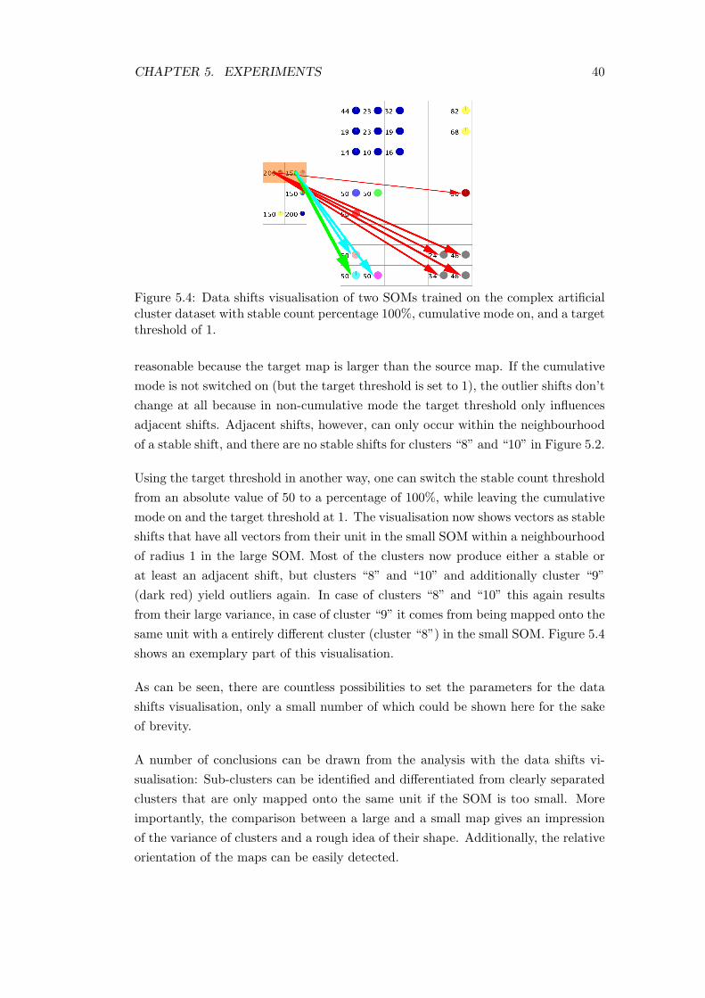
Figure 5.4: Data shifts visualisation of two SOMs trained on the complex artificialcluster dataset with stable count percentage 100%, cumulative mode on, and a targetthreshold of 1.

reasonable because the target map is larger than the source map. If the cumulativemode is not switched on (but the target threshold is set to 1), the outlier shifts don’tchange at all because in non-cumulative mode the target threshold only influencesadjacent shifts. Adjacent shifts, however, can only occur within the neighbourhoodof a stable shift, and there are no stable shifts for clusters “8” and “10” in Figure 5.2.

Using the target threshold in another way, one can switch the stable count thresholdfrom an absolute value of 50 to a percentage of 100%, while leaving the cumulativemode on and the target threshold at 1. The visualisation now shows vectors as stableshifts that have all vectors from their unit in the small SOM within a neighbourhoodof radius 1 in the large SOM. Most of the clusters now produce either a stable orat least an adjacent shift, but clusters “8” and “10” and additionally cluster “9”(dark red) yield outliers again. In case of clusters “8” and “10” this again resultsfrom their large variance, in case of cluster “9” it comes from being mapped onto thesame unit with a entirely different cluster (cluster “8”) in the small SOM. Figure 5.4shows an exemplary part of this visualisation.

As can be seen, there are countless possibilities to set the parameters for the datashifts visualisation, only a small number of which could be shown here for the sakeof brevity.

A number of conclusions can be drawn from the analysis with the data shifts vi-sualisation: Sub-clusters can be identified and differentiated from clearly separatedclusters that are only mapped onto the same unit if the SOM is too small. Moreimportantly, the comparison between a large and a small map gives an impressionof the variance of clusters and a rough idea of their shape. Additionally, the relativeorientation of the maps can be easily detected.


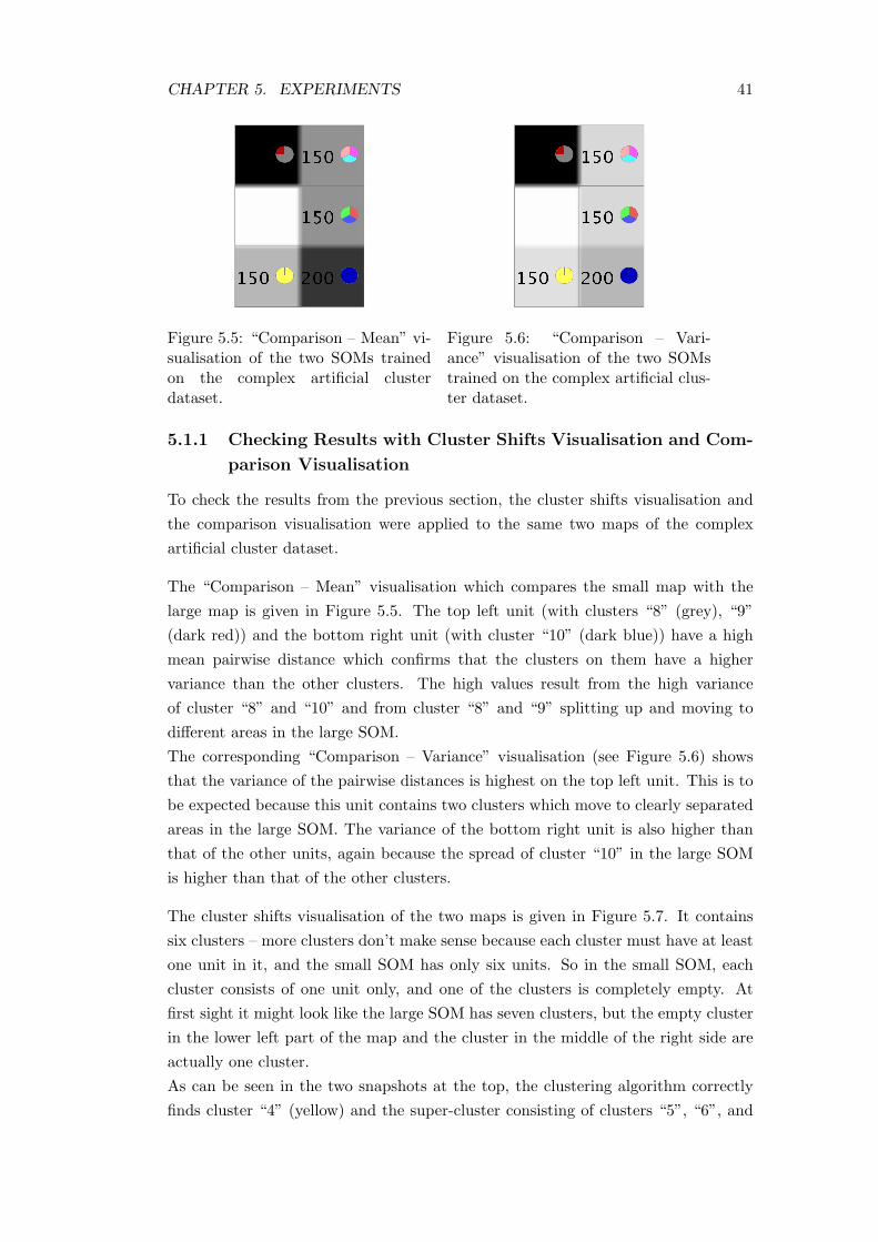
Figure 5.5: “Comparison – Mean” vi-sualisation of the two SOMs trainedon the complex artificial clusterdataset.

Figure 5.6: “Comparison – Vari-ance” visualisation of the two SOMstrained on the complex artificial clus-ter dataset.

5.1.1 Checking Results with Cluster Shifts Visualisation and Com-

parison Visualisation

To check the results from the previous section, the cluster shifts visualisation andthe comparison visualisation were applied to the same two maps of the complexartificial cluster dataset.

The “Comparison – Mean” visualisation which compares the small map with thelarge map is given in Figure 5.5. The top left unit (with clusters “8” (grey), “9”(dark red)) and the bottom right unit (with cluster “10” (dark blue)) have a highmean pairwise distance which confirms that the clusters on them have a highervariance than the other clusters. The high values result from the high varianceof cluster “8” and “10” and from cluster “8” and “9” splitting up and moving todifferent areas in the large SOM.The corresponding “Comparison – Variance” visualisation (see Figure 5.6) showsthat the variance of the pairwise distances is highest on the top left unit. This is tobe expected because this unit contains two clusters which move to clearly separatedareas in the large SOM. The variance of the bottom right unit is also higher thanthat of the other units, again because the spread of cluster “10” in the large SOMis higher than that of the other clusters.

The cluster shifts visualisation of the two maps is given in Figure 5.7. It containssix clusters – more clusters don’t make sense because each cluster must have at leastone unit in it, and the small SOM has only six units. So in the small SOM, eachcluster consists of one unit only, and one of the clusters is completely empty. Atfirst sight it might look like the large SOM has seven clusters, but the empty clusterin the lower left part of the map and the cluster in the middle of the right side areactually one cluster.As can be seen in the two snapshots at the top, the clustering algorithm correctlyfinds cluster “4” (yellow) and the super-cluster consisting of clusters “5”, “6”, and


Figure 5.7: Cluster shifts visualisation of two SOMs trained on the complex artificialcluster dataset.

“7”. It also finds the super-cluster of clusters “1”, “2”, and “3”, which is not shownin Figure 5.7 because it looks very similar to the top right snapshot. Cluster “10” isalso identified, see the bottom left snapshot. However, there is a cluster shift outlierin the bottom right snapshot: The vectors from clusters “8” and “9” come to lie inone unit / cluster in the small SOM, but are recognised as separate clusters in thelarge SOM. The data vectors from cluster “9” are marked as outliers because theircluster is identified with the empty cluster in the small SOM. A correct identificationisn’t possible here because the cluster mapping is always 1 to 1 and clusters “8” and“9” will always be mapped into the same cluster in the small SOM.

So the clustering algorithm correctly finds all (super-)clusters and the cluster as-signment scheme correctly identifies clusters where it is possible. Together with theresults from the comparison visualisations about the clusters’ variance, this rein-forces the findings of the data shifts visualisations.


0 1 2 3 4 5 6 7 8Lowest 68% 52% 81% 59% 70% 95% 97% 94% 100%Medium 88% 78% 86% 82% 84% 97% 97% 100% 100%Highest 94% 99% 99% 100% 97% 99% 100% 100% 100%Average 83% 76% 89% 80% 84% 97% 98% 98% 100%

Table 5.1: Cluster assignment confidences for SOMs trained on equidistant Gaussiancluster datasets “0” through “8”.

5.2 Cluster Shifts Visualisation on the Equidistant Gaus-

sian Cluster Datasets

The cluster shifts visualisation, particularly the cluster assignment method, wastested using the “equidistant Gaussian cluster datasets” described in Section 4.1.They contain samples from three equidistant 2-dimensional Gaussian distributions;the distance between the Gaussian centres (means) increases from 0 in dataset “0”to 10 in dataset “10”.For each of the datasets “0” through “8”, two SOMs were trained with exactly thesame parameters: a map size of 10× 10, an initial learning rate α0 = 0.75, an initialneighbourhood size σ0 = 10 and 10,000 iterations. Only the random seed for theinitialisation of the prototype vectors differed between both SOMs, being 42 for oneand 421 for the other.The resulting two SOMs for each dataset were then compared with each other.They were clustered into three clusters (because the data contains three classes) withhierarchical clustering, using Ward’s linkage function, and the clusters in both SOMswere assigned to each other. This yielded three cluster assignment confidences perdataset (one for each cluster pair). As described in Section 3.2.1, the “confidence”is the percentage of data vectors that moved from a cluster in the first SOM toa cluster in the second SOM. The highest, lowest and average cluster assignmentconfidence for datasets “0” through “8” are detailed in Table 5.1 and plotted inFigure 5.8.Naturally, the confidences increase the farther apart the Gaussian centres get.That the confidences get very close to 100% around dataset “5” and “6” is also notsurprising, given the structure of the data. In dataset “6”, the samples of differentclasses are (almost) completely separated because the 3σ radiuses of the Gaussiansdon’t overlap (see Section 4.1 for a more detailed explanation). Thus the clusteringalgorithm always finds clusters almost perfectly corresponding to the classes and toeach other.

A subset of the produced cluster shifts visualisations is shown in Figure 5.9. Itcontains the visualisations for datasets (top to bottom) “0”, “2”, “4”, and “6” – seeFigure 4.1 for plots of the original data.


Figure 5.8: Cluster assignment confidences for SOMs trained on equidistant Gaus-sian cluster datasets “0” through “8”.

In the topmost figure, the one for dataset “0”, it is obvious that the different classesare mixed up randomly on both SOMs, just as is to be expected from the data.The clusters are, of course, also built rather randomly, so the cluster assignmentconfidences are relatively low, averaging to 83% (compare Figure 5.8 and Table 5.8).The confidences are as high as 83% (which isn’t bad for other datasets which arenot built artificially) because the clustering algorithm detects similar areas in dataspace as clusters in both SOMs – only the right SOM is turned upside down incomparison to the left SOM. As the clusters are so random and don’t correspond toa single class each, it can’t be verified if the clusters that correspond to a class aremapped onto each other.In the next figure, based on dataset “2”, the classes start to separate, moving intodifferent corners of the SOM. The clusters aren’t so random any more – one can makeout a yellow, a green, and a red cluster (although there are errors, of course). Theyellow, green, and red clusters are correctly mapped onto each other, the averageconfidence increases to almost 90%.The third figure (for dataset “4”) shows quite well-separated classes, but the cluster-ing algorithm doesn’t find the clusters corresponding to the classes perfectly. Thereare errors along the class borders, the clustering is unprecise in separating the classes,thus the the average cluster assignment confidence decreases to 84%.The last figure (for dataset “6”) shows clearly separated classes, no data vectorsfrom different classes are mapped onto the same unit. The clustering is still a bitunprecise, however, the average cluster assignment confidence rises to almost 100%.(The cluster assignment confidence finally reaches 100% in dataset “8”.)

Apparently, the cluster assignment method works well. Where there are clusters


Figure 5.9: Cluster shift comparisons between pairs of SOMs trained on the samedatasets. The datasets are the equidistant Gaussian cluster sets (top to bottom)“0”, “2”, “4”, and “6” (see Figure 4.1).


Figure 5.10: “Comparison – Mean”visualisation of the two SOMs trainedon equidistant Gaussian clusterdataset “0”.

Figure 5.11: “Comparison – Mean”visualisation of the two SOMs trainedon equidistant Gaussian clusterdataset “6”.

corresponding to the classes, the right clusters are identified with each other, sothat the “green” cluster in the left SOM is always mapped onto the “green” clusterin the right SOM, and so on. The confidence value roughly corresponds to the gradeof separation of the clusters and thus to the “cleanness” of the clusters.

5.2.1 Checking Results with Data Shifts Visualisation and Com-

parison Visualisation

The equidistant Gaussian clusters datasets were also tested with the other visuali-sations to check whether their results would support the findings from the previoussection.Figure 5.10 and 5.11 show two “Comparison – Mean” visualisations for two pairs ofSOMs trained on the equidistant Gaussian cluster datasets “0” and “6” respectively.The maps are the ones used for Figure 5.9 in the previous section.When comparing the two comparison visualisations there are two interesting differ-ences:Firstly, while in Figure 5.10 there are a lot of grey units (with a low mean pairwisedistance) in the centre of the map, Figure 5.11 has very few units with a mean pair-wise distance greater than zero in its centre. This may seem trivial, as in Figure 5.11the clusters are already well-separated and the area in the centre is therefore sparseof data vectors. There is a Y-shaped rift between the clusters where the units havevery few data vectors or none at all. So the grade of cluster separation is visible inthese two comparison visualisations, too.Secondly, there are a lot more units with a mean pairwise distance of zero in Fig-ure 5.11 than in Figure 5.10. This probably results from the fact that dataset “6”has a clear inner structure (three distinct clusters) while dataset “0” consists onlyof one big Gaussian cluster. As dataset “0” has little structure, the fit of SOMs to


Figure 5.12: Data shift comparisons between pairs of SOMs trained on the equidis-tant Gaussian cluster datasets “0” (top) and “6” (bottom).

the input data depends a lot on their random initialisation, so the resulting SOMsdiffer. On the other hand, dataset “6” has a clear structure to which each SOM canfit, making the differences between SOMs with different random initialisations muchsmaller.

The structure of the input data also becomes visible in parts of the data shiftsvisualisations of the same SOMs. Figure 5.12 shows these visualisations where thetwo middle rows of units in each SOM are selected. The data vectors from theselections behave differently in both maps. For the maps trained on dataset “0”, thedata vectors scatter widely on the right SOM. For the maps trained on dataset “6”,however, the data vectors are mapped into the two middle columns of the right mapalmost perfectly. Taking into account the mirrored orientation of the two SOMs,this means that the same data vectors get mapped to almost the same positions inthose two maps.

So the data shifts and comparison visualisations back up each other and confirm thefindings from the cluster shifts visualisation.


Figure 5.13: “Comparison – Mean” (top) and “Comparison – Variance” (bottom)visualisations for two SOMs trained on the intertwined rings dataset.

5.3 Comparison Visualisation on the Intertwined Rings

Dataset

A useful application for the comparison visualisation is the detection of breaches intopology, which it can show by a high mean distance on a unit or area while thesurrounding units have a low mean distance. In order to test this, the “intertwinedrings dataset” was used (see Section 4.2).Eight SOMs were trained on it with a size of 20 × 10 units, initial neighbourhoodsize σ0 = 10, initial learning rate α0 = 0.75, and 10,000 iterations. The random seeddiffered in order to produce different projections, being 42, 21, 3515, 58, 486, 789,8, and 999 respectively for SOMs “1”, “2”, “3”, “4”, “5”, “6”, “7”, and “8”.The analysis was started by comparing SOM “1” with the SOM “3” using the“Comparison – Mean” and the “Comparison – Variance” visualisation. The results,


showing SOM “1” with a class information visualisation put on top, can be seen inFigure 5.13.Obviously, the two rings were broken during the projection. However, there is nounit with samples from both classes mapped onto it, rather the two classes aremapped into well-separated connected areas that can be seen as broken circles.The “Comparison – Mean” visualisation mostly shows low to medium values for themean distance, but two units in the middle of the SOM catch the eye immediatelybecause of their very high mean distance value (which makes them black). Whenlooking a the “Comparison - Variance” visualisation, it becomes clear that these twounits are the only ones to have significant variance. It can be suspected that thebreach in topology that results from breaking the rings occurs at these locations inthe data space – in the other SOM, SOM “3”.In order to minimise the influence of small pairwise distances of vectors (resultingfrom vectors being mapped onto neighbouring units) the threshold in the “Compar-ison – Mean” visualisation was set to 3. This means that the pairwise euclideandistance between two vectors in SOM “3” (which lie on the same unit in SOM “1”)must be more than 3 to count towards the mean distance. The result should be thatonly vectors that moved very far away from each other show up in the visualisation.Sure enough, only the two noticeable units have a mean distance greater than zerowith this setting.To see what happens with the data vectors from these units, the data shifts visual-isation was employed and put on top of the “Comparison – Variance” visualisation.(The parameters for the data shifts visualisation are not very important here butare given nonetheless: source threshold: 1, target threshold: 1, cumulative “on”,absolute count thresholds: stable: 5, outlier: 1.)Figure 5.14 shows two snapshots of the combined visualisation. The upper snapshotshows the data shifts for the area around the upper unit of interest (highlighted inorange); SOM “3” is displayed at the top and SOM “1” below it. As was suspected,this unit marks the location in the data space where the “red” ring is broken inSOM “3”. The same is true for the lower unit of interest and the “blue” ring, ascan be seen in the lower snapshot.

To further test the capabilities of the comparison visualisation, SOM “1” was thencompared not only with SOM “3” but with all other seven SOMs, the thresholdagain set to 3. The resulting “Comparison – Variance” visualisation (combined withthe class information) can be seen in Figure 5.15.This visualisation now shows not only two areas of interest but five: the two in themiddle already seen in the previous visualisations and additionally two at the endsof the blue conglomerate and one at the lower end of the red conglomerate.It appears that these points of interest mark the breakage points of the rings whichare most likely to be generated by SOMs. There are two breakage points on each


Figure 5.14: Combined data shifts and comparison visualisations for the intertwinedrings dataset.


Figure 5.15: “Comparison – Variance” visualisation for eight SOMs trained on theintertwined rings dataset.

Figure 5.16: Plot of the input space for the intertwined rings dataset with the pointsof interest marked in green.


ring and they are symmetrical.To check this hypothesis, the vectors on the units of interest can be marked inthe plot of the original data, which results in Figure 5.16 (markers in green). Andindeed, they show up as symmetrical points, one on each half circle, although thetwo ends of the blue conglomerate (which end up on the “upper” half of the bluering in the plot) do not overlap as nicely as one might expect.When looking back to Figure 5.14 it becomes clear that SOM “1” produced just themirror images of both breakage points in SOM “3”.

5.3.1 Checking Results with Data Shifts Visualisation and Cluster

Shifts Visualisation

The intertwined rings dataset was checked also with the data shifts and the clustershifts visualisations. Interesting findings of the data shifts visualisation were alreadygiven above in Figure 5.14: The breaches in topology become visible in the data shiftsvisualisation.Apart from the breaking points of the rings, the topology is preserved well by theSOMs’ projections, as can be seen from the comparison visualisation with low meanpairwise distances (see Figure 5.13). This is supported by another data shifts visu-alisation, see Figure 5.17, which compares SOM “1” (above) with SOM “3” (below)(and has the same parameters as Figure 5.14). The data vectors from a continuousconnected area in one SOM move to a similar area in the second SOM. The ringsare rotated in comparison to each other, but the data vectors remain within theirsmall neighbourhoods in both SOMs. For clarity, only a part of the data shifts isshown in the figure, but the other shifts look similar.

A cluster shifts visualisation on the same two maps also yields interesting results,see Figure 5.18. When clustering the map into two clusters, each cluster holds themajority of data vectors from one ring and a small part of the other ring. Thisis to be expected because the intertwined rings dataset is not linearly separable.When separating the 3-dimensional rings by a plane, a small portion of each ringwill always be cut off and assigned to the cluster of the other ring. In SOM “1”, thecluster borders run through the points where the breaches in topology occur, thepoints where the rings are broken up in SOM “3”. The breakage area of the bluering is selected (marked in orange) in Figure 5.18. The breakage area for the redring isn’t shown but looks analogue.

Apparently, the data shifts and cluster shifts visualisations back up the results fromthe comparison visualisation about the breaches in the rings’ topology.


Figure 5.17: Data shifts visualisation of two SOMs trained on the intertwined ringsdataset.

Figure 5.18: Cluster shifts visualisation of two SOMs trained on the intertwinedrings dataset.


5.4 Assessing SOM Quality on Equidistant Gaussian

Cluster Dataset “5”

To test how the proposed visualisations display differences in SOM quality, eight“well-trained” and two “badly-trained” SOMs were built on the equidistant Gaussiancluster dataset “5”, which contains 3 equidistant Gaussian clusters with distance 5(see Section 4.1).The parameters for the badly-trained maps were tweaked to impede a perfect fit ofthe map to the data, while the parameters of the well-trained maps were set to allowfor a good fit to the data. The parameters that were the same for all maps were: amap size of 6× 6 units, an initial learning rate of α0 = 0.75, and 500 training steps.The maps differed in their random seeds (to guarantee their independence) and theirinitial neighbourhood size (to tweak their fit to the data): The random seeds were1807, 4209, 289, 2431, 4571, 2079, 3506, 4659, 1185, and 4088 respectively. Theinitial neighbourhood size σ0 was 6 for SOMs “1” to “8” (well-trained) and 2 and1 respectively for SOMs “9” and “10” (badly-trained). The small neighbourhoodsizes were chosen to enforce errors in the SOMs’ preservation of topology.The maps were then analysed and compared with the help of the three visualisations.

5.4.1 Data Shifts Visualisation

Of the many possible combinations of maps for data shifts visualisations, two wereselected: A badly-trained map and a well-trained map were both compared withanother well-trained map. Figure 5.19 shows the resulting two data shifts visuali-sations: At the top, SOM “10” (badly-trained) is compared with SOM “5” (well-trained); at the bottom, SOM “1” (well-trained) is also compared with SOM “5”.The visualisations’ parameter settings were: Cumulative mode on, source thresh-old: 1, target threshold 1, absolute stable count threshold: 5, absolute outlier countthreshold: 1.The first snapshot shows that the data vectors from the two middle rows of SOM“10” spread over almost the whole map in SOM “5”. Apparently, the two SOMsdon’t represent the input data in a similar way, which is a hint that at least one ofthe maps doesn’t fit the data optimally.The second snapshot, however, reveals that the vectors from the two middle rowsfrom SOM “1” are mapped (almost perfectly) to the two middle columns of SOM“5”. This indicates that the SOMs’ orientations are mirrored in comparison to eachother and that they both represent the data’s inner structure in a similar way.So two SOMs (“1” and “5”) represent the input data in a similar way while thethird SOM differs from them. This suggests that SOMs “1” and “5” fit better tothe input data than SOM “10” – if they aren’t somehow similar by accident, whichmay be ruled out by comparing more SOMs with varying parameters with them.


Figure 5.19: Data shifts visualisation of SOMs trained on equidistant Gaussiancluster dataset “5”, comparing SOMs “10” and “5” (top) and “1” and “5” (bottom).


Figure 5.20: Cluster shifts visualisation of SOMs trained on equidistant Gaussiancluster dataset “5”, comparing SOMs “1” and “10”.

Thus, it gives an indication for the SOMs’ quality.

5.4.2 Cluster Shifts Visualisation

A cluster shifts visualisation with the number of clusters set to three was done next.It compares SOMs “1” (well-trained) and “10” (badly-trained), see Figure 5.20. Thedifferent shape of the clusters in the two SOMs gives a strong indication that theydon’t represent the input data in a similar way. In SOM “1”, three about equallysized and shaped clusters lie in three parts of the map. In SOM “10” there are twosmall and one large cluster, all with a different shape, and the large cluster claspsaround one of the small clusters. The question is, which of the maps represents thedata’s structure better. It may be the case that SOM “1” oversimplifies the inputdata’s inner structure into three similarly shaped clusters, but it seems more likelythat the obscure shapes of the clusters in SOM “10” are the result of a badly trainedmap, especially as the units on the right-hand side border of SOM “10” have almostno data vectors mapped to them.So, comparing the shapes of corresponding clusters in different SOMs may indicatethe SOMs’ quality as well.

5.4.3 Comparison Visualisation

Finally, four “Comparison – Mean” visualisations were generated, which compare theSOMs “1”, “5”, “9”, and “10” respectively with all other SOMs. The visualisationsare shown in Figure 5.21. It becomes apparent that the well-trained maps (“1” and“5”) have very few units with high mean pairwise distances and a lot of units withlow and approximately equal mean pairwise distances. (The units with no or onlyone data vector on them of course have a mean pairwise distance of 0 and shouldbe disregarded here.) The badly-trained maps (“9” and “10”) have more units with


Figure 5.21: “Comparison – Mean” visualisations on ten SOMs trained on equidis-tant Gaussian cluster dataset “5”. Top left: SOM “1”, top right: SOM “5”, bottomleft: SOM “9”, bottom right: SOM “10”.


Figure 5.22: ‘‘Comparison – Mean” visualisations on four SOMs trained on equidistant Gaussiancluster dataset “5”.]“Comparison – Mean” visualisations on four SOMs trained onequidistant Gaussian cluster dataset “5”. Top left: SOM “1”, top right: SOM “5”,bottom left: SOM “9”, bottom right: SOM “10”..

high mean distances and more variation of values between the units. Apparently, thevariation between the units of the same map is lower for the good maps and higher forthe bad maps. This seems logical because good maps should fit well to the input dataand thus be very similar, whereas in the bad maps the influence of random factorsand parameter settings is higher, which produces inhomogenous maps. (Rememberthat the colours can’t be compared directly between the visualisations, but that thevariation within a map can, of course, be read from each visualisation.)So it is possible here to discern good and bad maps by looking at the comparisonvisualisations and finding a high variation between the units there. This is also trueif the proportion of good maps in the comparison is smaller. In the above case, theset of compared SOMs contained eight good maps and two bad maps. However,the results are similar if it contains only two good maps and two bad maps, as canbe seen in Figure 5.22. But if there is only one good map in three bad maps, for


example, the distinction can’t be made anymore just from looking at the comparisonvisualisation, so this method has its limits.

All in all, it seems that the three visualisations can be used to asses SOM quality, toindicate which of a set of compared maps are better and which are worse. However,all three visualisations compare SOMs with each other and don’t compare the mapin the output space with the input data. So all indications of quality are relative tothe compared maps and not absolute. To get an absolute measurement of a SOM’sfit to its input data, quality measures like those mentioned in Section 2.4 can beused.

5.5 Test on Real-life Data: Iris Dataset

A test on real-life data was done for all three visualisations with the Iris dataset (seeSection 4.4). Two maps were trained on the data, both with an initial learning rateα0 = 0.75, 10,000 iterations and a random seed for prototype vector initialisation of42, though with different sizes and initial neighbourhood sizes: one with 5× 5 unitsand σ0 = 5 and the other with 10× 10 units and σ0 = 10.Then both maps were compared with all three visualisations to find out how thedata vectors moved, and what the differences and similarities of the maps are.

5.5.1 Data Shifts Visualisation

First, a data shifts visualisation was done with the following parameters:

• A source threshold of 0 and a target threshold of 1, to account for the farbigger size of the second map: Of course, the data vectors will have moreunits to spread over in the second SOM, so the neighbourhood for the secondSOM must naturally be larger.

• The cumulative option switched on, to make full use of the target neighbour-hood radius (target threshold) in the second SOM.

• An absolute count threshold of 4 for stable shifts and 1 for outlier shifts,because the minimum number of data vectors on a unit in the smaller SOM is3, and 4 is just a bit above it.

Information about the data vectors’ classes was added to the visualisations, revealingthe real inner structure of the data. The setosa class is marked in yellow, theversicolor class in dark blue, and the virginica class in light blue. This shows thatthe position of the data on the second map is mirrored in comparison to the firstmap.


Figure 5.23: Data shifts visualisation: data vectors from the setosa class spread overmore units in a larger SOM.


Figure 5.24: Data shifts visualisation: Data vectors from the core of the virginicaclass.

Figure 5.25: Data shifts visualisation: All outlier shifts in the data shifts visualisa-tion.


Interesting results can be seen when looking at the setosa class (see Figure 5.23). Its50 vectors all amass on 3 units in the top left corner of the small map, with a gapof empty units (onto which no data vectors were mapped) around them. Similarly,on the large map, the vectors come to lie in a clearly separated, elongated area onthe right-hand border. The gap shows that the setosa samples separate themselvesclearly from the other two classes (this is confirmed by looking at the statisticalanalysis of the Iris dataset [4]). The data shifts visualisation also shows how nicelythe topology of the data is preserved in both SOMs: The vectors from the rightmostsetosa unit in the small map is mapped onto the top of the elongated setosa area inthe large map; the vectors from the middle unit in the small map are mapped ontothe middle of the elongated area in the large map; and the vectors on the leftmostunit are mapped onto the bottom of the elongated area. This fits perfectly to themirrored orientation of the SOMs.The cohesive core of the virginica area is also clearly preserved in both SOMs, thoughits topological structure isn’t repeated in both SOMs as strongly as with the setosaclass. See Figure 5.24 for the mapping between the two SOMs.The borders of the virginica area and the versicolor area, however, are not as cohesiveand spread over a wider area than the other two classes. Figure 5.25 shows only theoutlier shifts for the data shifts visualisation of the two SOMs. Most of the outliershifts emerge from units in the versicolor area or the border of the virginica area.The conclusion that can be drawn is that the setosa class and the core of the virginicaclass seem to be projected onto the SOMs’ grids in a way that preserves the topologywell, and the distinction between the setosa class and the other two classes is veryclear. The borders of the virginica class and the versicolor class, however, overlapand are rendered differently on both maps.

5.5.2 Cluster Shifts Visualisation

To further investigate the properties of the dataset, the cluster shifts visualisationwas used. Different numbers of clusters were tried out on the two SOMs: Figure 5.26shows three different cluster visualisations with two, three, and four clusters respec-tively (from top to bottom).If the number of clusters is two, the clustering algorithm puts all setosa samplesinto one cluster and all versicolor and virginica samples into the other cluster. Thecluster assignment confidence here is 100% for both mappings. This, again, showsthat the setosa class is clearly distinct from the other two, while versicolor andvirginica are overlapping.For the next case, if there are three clusters, all possible mappings and their con-fidences are given in Table 5.2. The setosa cluster is still the same as before andits mapping has 100% confidence. The other two clusters each represent one of theother two classes in the small map, but in the large map the virginica cluster gets


Figure 5.26: Cluster shifts visualisations of the Iris dataset with 2, 3, and 4 clusters(top to bottom).


Cluster in 1st SOM Cluster in 2nd SOM Confidencesetosa setosa 100%virginica virginica 100%versicolor versicolor 69%versicolor virginica 31%all others 0%

Table 5.2: Cluster assignment confidences for two maps trained on the Iris dataset,clustered into three clusters.

Cluster in 1st SOM Cluster in 2nd SOM Confidencesetosa setosa 100%virginica core virginica core 100%versicolor/virginica versicolor/virginica 74%versicolor versicolor 69%versicolor versicolor/virginica 31%versicolor/virginica virginica core 26%all others 0%

Table 5.3: Cluster assignment confidences for two maps trained on the Iris dataset,clustered into four clusters.

assigned quite a few versicolor samples as well. These show up as the outlier shiftsdrawn in in red. The virginica clusters’ assignment confidence is 100%, the versicolorclusters’ confidence is only 69%.This points to a weakness in the confidence measure which only considers the direc-tion from the first (the small) to the second (the large) map, and not both ways.The problem may be alleviated by changing the confidence measures as proposed inChapter 6.The last snapshot shows the cluster shifts visualisation with four clusters (with nostable or outlier shifts drawn in). All possible mappings and their confidences aregiven in Table 5.3. There is one cluster for the setosa class (assignment confidence100%), one cluster for the core of the virginica class (assignment confidence 100%),one cluster for the versicolor class (assignment confidence 69%), and one clusterfor the border between versicolor and virginica (assignment confidence 74%). Thisshows again that at their borders the versicolor class and virginica class are hard todistinguish.

5.5.3 Comparison Visualisation

Finally, a comparison visualisation (“Comparison – Mean”) was used to find theunits in the smaller SOM where the projection onto the two-dimensional SOM-gridis unstable – see Figure 5.27. The minimum pairwise distance threshold was setto 2.5, to reduce the impact of the bigger size of the larger SOM: The data vectors


Figure 5.27: “Comparison – Mean” visualisation of the Iris dataset.

spread over more units in the larger SOM, thus the vectors that lie on one unit in thesmall SOM will spread over a couple of neighbouring units in the large SOM. Thiswill distort the conclusions we wish to draw from the visualisation, so the thresholdis used to compensate for the spread.The units with the high mean pairwise distances (marked in shades of grey) all areeither on the border between the versicolor and virginica classes or within the versi-color class. This points to the relative instability of the projection of the versicolorclass onto the SOM-grid: data vectors from the versicolor class are projected dif-ferently in both SOMs. Yet again, these results suggest that the setosa class andto some extend the core of the virginica class are well-defined and distinct, whilethe border between virginica and versicolor and versicolor class itself are a relativelyunstable area in a SOM projection.So the results from the three visualisations support and reinforce each other – andthus may allow to draw useful conclusions for other, not so well-known datasets aswell.

5.6 Summary

This chapter described the experiments conducted on the visualisations introducedin Chapter 3 on the datasets from Chapter 4.It was found that they can be used to detect differences between the projectionsof two or more different SOMs, breaches in topology, rotations and reflections ofSOMs relative to each other, clusters and sub-clusters, and clusters correspondingto each other. They give indications on the compared SOMs’ relative quality, seemto support and reinforce each other’s findings and may be useful to explore otherdatasets.

Chapter 6

Future Work

The visualisations described in this work may prove useful but surely can be im-proved upon to work faster, better, or give the user more options to fine-tune thevisualisations’ results.This chapter gives a few ideas and suggestions on possible improvements that couldbe useful.

• The data shifts visualisation could be extended by making the neighbourhoodsmore user-adjustable. Currently, the neighbourhoods can differ in size/radius,but will always be circular. Other shapes of neighbourhoods could be added.Also, instead of defining the neighbourhood through shape and radius, onecould just take the k nearest neighbours and use them as a neighbourhood.

• To improve the cluster shifts visualisation, different methods for establishingthe confidence of a the cluster mapping could be tried out. Instead of com-puting the percentage of data vectors which moved from a cluster in the firstSOM to a cluster in the second SOM, one could do it the other way round:compute the percentage of data vectors which moved from a cluster in thesecond SOM to a cluster in the first SOM. Or one could combine these twomeasures, possibly weighing them differently. This may result in a confidencemeasure more closely reflecting the similarity of the clusters but may increasethe computational cost.

• Another way to improve the cluster mapping could be to change the methodby which the entries from the table of confidences are picked. Instead ofalways choosing the highest available confidence, one could use an optimisationalgorithm to maximise the overall sum of confidences. This could achievebetter cluster mappings.

• The comparison visualisation could be extended by adding other distance func-tions to compute pairwise distances between vectors. For the cluster distance

66

CHAPTER 6. FUTURE WORK 67

measure, other linkage functions such as complete linkage or average linkagecould be tried out.

Of course this list is by no means exhaustive or claims to tackle all problems that mayarise with the visualisations. It is merely a starting point for further development.

Chapter 7

Conclusion

This work introduced three new Self-organising Map visualisations which enablethe user to compare two or more SOMs trained on the same data with differentparameters: The data shifts visualisation, the cluster shifts visualisation and thecomparison visualisation. Datasets were constructed to test the new visualisations.Experiments were conducted and analysed, and it was found that the visualisationscan be helpful in determining the influence of parameter choice on the SOMs; theycan be employed for finding breaches in topology or areas in the SOMs were theprojection onto two dimensions is unstable and ambiguous. Likewise, particularlystable mappings which preserve the topology in the original data space especiallywell can be discovered.During the experiments, possibilities for enhancement of the visualisations becameapparent and solutions were proposed.All in all, the proposed visualisations can be used in data exploration to gain knowl-edge about datasets and especially about SOMs trained on that data.

68

List of Tables

3.1 Table of confidences for two SOMs trained on the data set describedin Section 4.2. . . . . . . . . . . . . . . . . . . . . . . . . . . . . . . 24

3.2 Final cluster assignment resulting from Table 3.1. . . . . . . . . . . . 24

4.1 Coordinates of the cluster centres of the equidistant Gaussian clusterdatasets. . . . . . . . . . . . . . . . . . . . . . . . . . . . . . . . . . . 32

5.1 Cluster assignment confidences for SOMs trained on equidistant Gaus-sian cluster datasets “0” through “8”. . . . . . . . . . . . . . . . . . 43

5.2 Cluster assignment confidences for two maps trained on the Iris dataset,clustered into three clusters. . . . . . . . . . . . . . . . . . . . . . . . 64

5.3 Cluster assignment confidences for two maps trained on the Iris dataset,clustered into four clusters. . . . . . . . . . . . . . . . . . . . . . . . 64

69

List of Figures

2.1 A SOM’s prototype vectors in the input space before training. . . . . 82.2 A SOM’s prototype vectors in the input space after training. . . . . 82.3 Example of a U-matrix. . . . . . . . . . . . . . . . . . . . . . . . . . 92.4 Example of a hit histogram. . . . . . . . . . . . . . . . . . . . . . . . 92.5 Example of a Smoothed Data Histogram . . . . . . . . . . . . . . . . 102.6 Example of class information visualisation. . . . . . . . . . . . . . . 112.7 Example of SOM clustering. . . . . . . . . . . . . . . . . . . . . . . . 11

3.1 Comparison of the position of data vectors on two different SOMstrained on the same data with different parameters. . . . . . . . . . 16

3.2 Units that lie within a certain neighbourhood radius around a centre. 173.3 Part of a data shifts visualisation. . . . . . . . . . . . . . . . . . . . 213.4 A cluster shifts visualisation, showing two SOMs clustered into two

clusters each. . . . . . . . . . . . . . . . . . . . . . . . . . . . . . . . 233.5 Simplified visualisation of the cluster shifts example. . . . . . . . . . 253.6 Illustration of the cluster distance function. . . . . . . . . . . . . . . 293.7 Example of a “Comparison – Mean” visualisation. . . . . . . . . . . 293.8 Combined comparison and data shifts visualisation. . . . . . . . . . . 29

4.1 Equidistant Gaussian cluster datasets “0”, “2”, “4”, and “6”. . . . . 324.2 Intertwined Rings Dataset. . . . . . . . . . . . . . . . . . . . . . . . 334.3 Complex Artificial Cluster Dataset. . . . . . . . . . . . . . . . . . . . 34

5.1 Data shifts visualisation of two SOMs trained on the complex artificialcluster dataset. . . . . . . . . . . . . . . . . . . . . . . . . . . . . . . 37

5.2 Data shifts visualisation of two SOMs trained on the complex artificialcluster dataset with different stable count threshold. . . . . . . . . . 39

5.3 Data shifts visualisation of two SOMs trained on the complex artificialcluster dataset with stable count threshold of 50, cumulative mode on,and a target threshold of 1. . . . . . . . . . . . . . . . . . . . . . . . 39

5.4 Data shifts visualisation of two SOMs trained on the complex artificialcluster dataset with stable count percentage 100%, cumulative modeon, and a target threshold of 1. . . . . . . . . . . . . . . . . . . . . . 40

70

LIST OF FIGURES 71

5.5 “Comparison – Mean” visualisation of the two SOMs trained on thecomplex artificial cluster dataset. . . . . . . . . . . . . . . . . . . . . 41

5.6 “Comparison – Variance” visualisation of the two SOMs trained onthe complex artificial cluster dataset. . . . . . . . . . . . . . . . . . . 41

5.7 Cluster shifts visualisation of two SOMs trained on the complex arti-ficial cluster dataset. . . . . . . . . . . . . . . . . . . . . . . . . . . . 42

5.8 Cluster assignment confidences for SOMs trained on equidistant Gaus-sian cluster datasets “0” through “8”. . . . . . . . . . . . . . . . . . 44

5.9 Cluster shift comparisons between pairs of SOMs trained on the equidis-tant Gaussian cluster sets. . . . . . . . . . . . . . . . . . . . . . . . . 45

5.10 “Comparison – Mean” visualisation of the two SOMs trained onequidistant Gaussian cluster dataset “0”. . . . . . . . . . . . . . . . 46

5.11 “Comparison – Mean” visualisation of the two SOMs trained onequidistant Gaussian cluster dataset “6”. . . . . . . . . . . . . . . . 46

5.12 Data shift comparisons between pairs of SOMs trained on the equidis-tant Gaussian cluster sets. . . . . . . . . . . . . . . . . . . . . . . . . 47

5.13 “Comparison – Mean” and “Comparison – Variance” visualisationsfor two SOMs trained on the intertwined rings dataset. . . . . . . . . 48

5.14 Combined data shifts and comparison visualisations for the inter-twined rings dataset. . . . . . . . . . . . . . . . . . . . . . . . . . . . 50

5.15 “Comparison – Variance” visualisation for eight SOMs trained on theintertwined rings dataset. . . . . . . . . . . . . . . . . . . . . . . . . 51

5.16 Plot of the input space for the intertwined rings dataset. . . . . . . . 515.17 Data shifts visualisation of two SOMs trained on the intertwined rings

dataset. . . . . . . . . . . . . . . . . . . . . . . . . . . . . . . . . . . 535.18 Cluster shifts visualisation of two SOMs trained on the intertwined

rings dataset. . . . . . . . . . . . . . . . . . . . . . . . . . . . . . . . 535.19 Data shifts visualisation of SOMs trained on equidistant Gaussian

cluster dataset “5”. . . . . . . . . . . . . . . . . . . . . . . . . . . . . 555.20 Cluster shifts visualisation of SOMs trained on equidistant Gaussian

cluster dataset “5”. . . . . . . . . . . . . . . . . . . . . . . . . . . . . 565.21 “Comparison – Mean” visualisations on ten SOMs trained on equidis-

tant Gaussian cluster dataset “5”. . . . . . . . . . . . . . . . . . . . 575.22 ‘ . . . . . . . . . . . . . . . . . . . . . . . . . . . . . . . . . . . . . . 585.23 Data shifts visualisation: Data vectors from the setosa class spread

over more units in a larger SOM. . . . . . . . . . . . . . . . . . . . . 605.24 Data shifts visualisation: Data vectors from the core of the virginica

class. . . . . . . . . . . . . . . . . . . . . . . . . . . . . . . . . . . . . 615.25 Data shifts visualisation: All outlier shifts in the data shifts visuali-

sation. . . . . . . . . . . . . . . . . . . . . . . . . . . . . . . . . . . . 615.26 Cluster shifts visualisations of the Iris dataset with 2, 3, and 4 clusters. 63

LIST OF FIGURES 72

5.27 “Comparison – Mean” visualisation of the Iris dataset. . . . . . . . . 65

Bibliography

[1] Hans-Ulrich Bauer and Klaus R. Pawelzik. Quantifying the neighborhoodpreservation of self-organizing feature maps. IEEE Transactions on NeuralNetworks, 3(4):570–579, July 1992.

[2] Christopher M. Bishop. Neural Networks for Pattern Recognition. Oxford Uni-versity Press, 1995.

[3] Michael Dittenbach, Robert Neumayer, and Andreas Rauber. Playsom: An al-ternative approach to track selection and playlist generation in large music col-lections. In Proceedings of the First International Workshop of the EU Networkof Excellence DELOS on Audio-Visual Content and Information Visualizationin Digital Libraries (AVIVDiLib 2005), pages 226–235, Cortona, Italy, May 4-62005.

[4] Ronald A. Fisher. The use of multiple measurements in taxonomic problems.In Annual Eugenics, 7, Part II, pages 179–188, 1936.

[5] Teuvo Kohonen. Self-organized formation of topologically correct feature maps.Biological Cybernetics, 43:59–69, 1982.

[6] Teuvo Kohonen. Self-Organizing Maps. Springer, Berlin, Heidelberg, 1995.

[7] Joseph B. Kruskal and Myron Wish. Multidimensional scaling. Sage UniversityPaper Series on Quantitative Application in the Social Sciences, 1978.

[8] Elias Pampalk. Aligned self-organizing maps. In Proceedings of the Workshopon Self-Organizing Maps (WSOM’03), pages 185–190, Hibikino, Kitakyushu,Japan, September 11-14 2003. Kyushu Institute of Technology.

[9] Elias Pampalk, Werner Goebl, and Gerhard Widmer. Visualizing changes inthe structure of data for exploratory feature selection. In Proceedings of theNinth ACM SIGKDD International Conference on Knowledge Discovery andData Mining, pages 157–166, Washington DC, August 24-27 2003. ACM.

[10] Elias Pampalk, Andreas Rauber, and Dieter Merkl. Using smoothed data his-tograms for cluster visualization in self-organizing maps. In Proceedings of the

73

BIBLIOGRAPHY 74

Intl Conf on Artificial Neural Networks (ICANN 2002), pages 871–876, Madrid,Spain, August 27-30 2002.

[11] Georg Polzlbauer. Survey and comparison of quality measures for self-organizing maps. In Jan Paralic, Georg Polzlbauer, and Andreas Rauber, ed-itors, Proceedings of the Fifth Workshop on Data Analysis (WDA’04), pages67–82, Sliezsky dom, Vysoke Tatry, Slovakia, June 24–27 2004. Elfa AcademicPress.

[12] Angela Roiger. Analyzing, labeling and interacting with soms for knowledgemanagement. Master’s thesis, Department of Software Technology and Inter-active Systems, Vienna University of Technology, Vienna, March 2007.

[13] Pang-Ning Tan, Michael Steinbach, and Vipin Kumar. Introduction to DataMining. Addison-Wesley, 2006.

[14] Alfred Ultsch and H. Peter Siemon. Kohonen’s self-organizing feature maps forexploratory data analysis. In Proceedings of the International Neural NetworkConference (INNC’90), pages 305–308, Dordrecht, Netherlands, 1990. Kluwer.

[15] Alfred Ultsch and C. Vetter. Selforganizing feature maps versus statistical clus-tering: A benchmark. Technical Report 9, Dept. of Mathematics and ComputerScience, University of Marburg, Germany, 1994.

[16] Jarkko Venna and Samuel Kaski. Neighborhood preservation in nonlinearprojection methods: An experimental study. In Artificial Neural Networks—ICANN 2001, pages 485–491. Springer, Berlin, 2001.

[17] Juha Vesanto. Som-based data visualization methods. Intelligent Data Analysis,3(2):111–126, 1999.

[18] Juha Vesanto and Esa Alhoniemi. Clustering of the self-organizing map. IEEETransactions on Neural Networks, 11(3):586–600, May 2000.

[19] Juha Vesanto, Mika Sulkava, and Jaakko Hollmen. On the decomposition ofthe self-organizing map distortion measure. In Proceedings of the Workshop onSelf-Organizing Maps (WSOM’03), pages 11–16, Hibikino, Kitakyushu, Japan,September 2003. Kyushu Institute of Technology.

[20] Joe H. Ward. Hierarchical grouping to optimize an objective function. Journalof the American Statistical Association, 58(301):236–244, March 1963.

visualisations for comparing self-organising mapsandi/download/thesis/bau_thesis07.pdf ·...

Documents