1

Vision 2.1 Scenario Modeling System Limited Scope Release

General Model Documentation Addendum to ARB’s 2016 Mobile Source Strategy Document

February, 2017

2

Vision 2.1 Scenario Modeling System ARB’s Vision for Clean Air Framework1, released in 2012, was developed to enhance ARB’s ability to conduct transportation system-wide, multi-pollutant analysis to inform policy development. It allows for the evaluation of technology, fuel, and efficiency interactions across many source sectors and multiple pollutants. Measuring and analyzing the system-wide emissions impacts that stem from strategies in individual sectors requires a comprehensive approach that reflects real-world linkages. Initially based on the Argonne National Laboratory (ANL) national VISION model which only estimated on-road vehicle greenhouse gas (GHG) emissions using national average emission factors, ARB’s Vision 1.0 model included California-specific data and methodologies and expanded the ability of the model to estimate upstream and tailpipe emissions of both greenhouse gas (GHG) and criteria pollutants from the operation of light - and heavy- duty vehicles in California.

ARB staff continued building on the Vision 1.0 model framework, to develop the Vision 2.0 model, an updated and expanded emission estimation tool that can analyze multiple potential technology and fuel pathways for individual emission sources while collectively considering multiple sectors, fuels, and technologies in comprehensive scenarios to study different pathways to meeting California’s air quality and climate goals. The Vision 2.01 model, released in October 2015, was designed with a primary focus on mobile source sectors, but also seamlessly integrates other economic sectors including energy and fuel production, other non-energy sources, and energy use in buildings. The model uses ARB’s most recent official inventory data including a draft version of EMFAC20142, and also considers all adopted transportation, fuels, and related policies as listed in Appendix A. A detailed overview of the Vision 2.0 model was presented at a public workshop1 in March 2015.

Vision 2.0 is unique in that was designed to focus on California specific policy questions and metrics by incorporating ARB’s most recent inventory work such as EMFAC2014 and reflects all adopted policies. In addition, it is one of the few scenario tools that integrates greenhouse gas and criteria emissions to inform how air quality, climate, and petroleum reduction goals can be met. Vision 2.0 combines several modules that have the most detailed breakdowns of each sector by vocation, technology type, and emissions process, and go further by providing that detail at an enhanced spatial resolution that can be merged with roadway network models. The output from the modules can also be merged with information about the cost of technologies and infrastructure for an economic assessment of a policy.

After reviewing the inputs and assumptions in Vision 2.0, Staff reflected the latest planning assumptions including the final version of EMFAC2014, and updated scenario assumptions3 to develop the present Vision 2.1 model. Vision 2.1 has the same modeling structure as Vision 2.0 and is used for the May 2016 Mobile Source Strategy

1 Vision Scenario Planning: http://www.arb.ca.gov/planning/vision/vision.htm 2 EMFAC2014: http://www.arb.ca.gov/msei/categories.htm 3 Vision Model Update Memo: http://www.arb.ca.gov/planning/vision/docs/vision2.1lr_update_memo.pdf

3

assessment4.

The current release of the Vision 2.1 modeling system includes a suite of six model components (modules):

• Passenger Vehicle Module; • Heavy Duty Vehicle Module;

o Baseline, SIP Measures, and Cleaner Technologies and Fuels Scenarios o Expanded Heavy Duty Vehicle ZEV Scenario

• Off-Road Module (forklifts and airport ground support equipment); • Locomotive Module; • Ocean Going Vessels Module; and • Energy Module

The main purpose of this document is to focus on the scenarios illustrated in the Mobile Source Strategy document. The scenario concepts are translated into assumptions which are evaluated in the Vision 2.1 model. These assumptions, when run through the Vision modules, provide the emission reductions associated with each scenario or concept. While some of the measure concepts are more complex than the current emission inventory and Vision could fully reflect, staff strove to develop assumptions that are consistent with the intent of proposed actions. During the regulatory process, regulatory-specific inventories will be compiled based on detailed fleet information collected through the outreach process including the most up-to-date data.

4 2016 Mobile Source Strategy: http://www.arb.ca.gov/planning/sip/2016sip/2016mobsrc.htm

4

Vision 2.1 Model – General Methodology The Vision modeling system incorporates detailed data from ARB’s official mobile source inventories (e.g. EMFAC20142 and off-road5) into separate “vehicle fleet modules” where comprehensive scenarios can be run for individual mobile source sectors. The tank-to-wheel (TTW) energy demand and tailpipe emission outputs from the individual “vehicle fleet modules” are aggregated into a central “energy module” where input assumptions on fuel mix and supply are considered to estimate the well-to-tank (WTT) fuel production related emissions. Figure 1 shows the general framework of the Vision 2.1 model. For example, information about changing technology sales, how clean those technologies are, and any changes in the transportation system efficiency are input to specific “vehicle fleet modules”. The model evaluates the impact of the assumptions on the TTW emissions and the associated energy demand. The energy demand from the “vehicle fleet modules” is input to the energy module along with assumptions about the mix of fuels to estimate upstream WTT emissions. Combining the WTT and TTW outputs from the model provides the full well-to-wheel (WTW) impacts of the scenario assumptions on the energy needs and associated emissions.

Figure 1 Framework of Vision 2.1 Model

5 ARB Off-Road Mobile Source Inventories: http://www.arb.ca.gov/msei/categories.htm#offroad_motor_vehicles

5

On-road Vehicle Modules The Vision 2.1 passenger vehicle module (PVM) and heavy duty vehicle (HDV) modules are scenario planning tools for on-road vehicles. In general, the on-road vehicle fleet modules are best described as a scenario tool that uses official EMFAC2014 data as a baseline, then allows the user to modify vehicle population, VMT, efficiency or emissions factors. Scenarios with range of advanced technology introduction and penetration can be modeled to evaluate the impact of vehicle technology on emissions, fuel and energy demand. The PVM covers passenger cars and trucks less than 8,501 pounds (lbs) gross vehicle weight rating (GVWR) and buses, while the HDV model covers trucks with over 8,500 pounds (lbs) gross vehicle weight rating (GVWR). Motorcycles, motorhomes and motor coaches are not currently included in Vision. All baseline information, including vehicle population, activity, age distributions, and emissions are obtained directly from ARB’s EMFAC2014 model with VMT updated to reflect adopted Regional Transportation Plans (RTPs) and Sustainable Communities Strategies (SCSs). While both modules maintain the majority of specificity from EMFAC2014, speed bins and hourly data are aggregated. EMFAC2014 as Vision Baseline:

A special EMFAC2014 emission model output was generated as input to Vision. To be consistent with SIP planning inventory, VMT from 2015 FSTIP (Federal Statewide Transportation Improvement Program) for 17 MPOs and SCAG’s draft 2016 RTP/SCS was used as custom VMT inputs to EMFAC model run. For non-MPO regions, VMT was based on default EMFAC2014.

Table 1 EMFAC2014 Baseline Data used in Vision

Baseline Data Included Notes

PVM HDV Calendar Year 2010-2050 Season Summer Region Seven Geographic Areas, See Figure 2 Vehicle Type See Table 2 Model Year Vehicle/Chassis Model year

Population Daily population; vehicle population on any given day on road

Vehicle Miles Traveled Daily Trips Daily

Emissions (All processes including exhaust, evaporative, tire wear and brake wear)

Daily CH4, CO, CO2, HC, NOx, PM,

PM10, PM2.5, ROG, and TOG

emissions

Daily CO2, NOx, PM2.5, and ROG

emissions

Fuel Consumptions Daily

6

Table 2: Vehicle Categories in the PVM and HDV Modules

EMFAC Vehicle ID Vision Model Description

LDA PVM Light-Duty Automobiles (i.e. Passenger Cars) LDT1 PVM Light-Duty Trucks (0-3,750 lbs GVWR) LDT2 PVM Light-Duty Trucks (3,751-5,750 lbs GVWR) MDV PVM Medium-Duty Trucks (5,751-8,500 lbs GVWR) UBUS PVM Urban Buses SBUS PVM School Buses OBUS PVM Other Buses LHD1 HDV Light-Heavy-Duty Trucks (GVWR 8501-10000 lbs) LHD2 HDV Light-Heavy-Duty Trucks (GVWR 10001-14000 lbs) T6 Ag HDV Medium-Heavy Duty Diesel Agriculture Truck

T6 CAIRP heavy HDV Medium-Heavy Duty Diesel CA International Registration Plan Truck with GVWR>26000 lbs

T6 CAIRP small HDV Medium-Heavy Duty Diesel CA International Registration Plan Truck with GVWR<=26000 lbs

T6 instate construction heavy HDV Medium-Heavy Duty Diesel instate construction Truck with

GVWR>26000 lbs T6 instate construction small HDV Medium-Heavy Duty Diesel instate construction Truck with

GVWR<=26000 lbs T6 instate heavy HDV Medium-Heavy Duty Diesel instate Truck with GVWR>26000 lbs T6 instate small HDV Medium-Heavy Duty Diesel instate Truck with GVWR<=26000 lbs T6 OOS heavy HDV Medium-Heavy Duty Diesel Out-of-state Truck with GVWR>26000 lbs T6 OOS small HDV Medium-Heavy Duty Diesel Out-of-state Truck with GVWR<=26000 lbs T6 Public HDV Medium-Heavy Duty Diesel Public Fleet Truck T6 utility HDV Medium-Heavy Duty Diesel Utility Fleet Truck T6TS HDV Medium-Heavy Duty Gasoline Truck T7 Ag HDV Heavy-Heavy Duty Diesel Agriculture Truck T7 CAIRP HDV Heavy-Heavy Duty Diesel CA International Registration Plan Truck T7 CAIRP construction HDV Heavy-Heavy Duty Diesel CA International Registration Plan

Construction Truck T7 NNOOS HDV Heavy-Heavy Duty Diesel Non-Neighboring Out-of-state Truck T7 NOOS HDV Heavy-Heavy Duty Diesel Neighboring Out-of-state Truck T7 other port HDV Heavy-Heavy Duty Diesel Drayage Truck at Other Facilities T7 POAK HDV Heavy-Heavy Duty Diesel Drayage Truck in Bay Area T7 POLA HDV Heavy-Heavy Duty Diesel Drayage Truck near South Coast T7 Public HDV Heavy-Heavy Duty Diesel Public Fleet Truck T7 Single HDV Heavy-Heavy Duty Diesel Single Unit Truck T7 single construction HDV Heavy-Heavy Duty Diesel Single Unit Construction Truck T7 SWCV HDV Heavy-Heavy Duty Solid Waste Collection Truck T7 tractor HDV Heavy-Heavy Duty Diesel Tractor Truck T7 tractor construction HDV Heavy-Heavy Duty Diesel Tractor Construction Truck T7 utility HDV Heavy-Heavy Duty Diesel Utility Fleet Truck T7IS HDV Heavy-Heavy Duty Gasoline Truck PTO HDV Power Take Off

7

The special output also provides population, activity and emissions for natural gas powered trash trucks (T7 SWCV) and urban buses (UBUS). Table 1 outlines the data from EMFAC2014 model that were used in the development of the Vision 2.1 on-road baseline inventory. The on-road Vision vehicle categories listed in Table 2 are further split into the fuel technology categories shown in Table 3.

Table 3: Vehicle Technology Categories

Technology Description Model

EMFAC PVM HDV Gas Gasoline Fueled Vehicles x x x DSL Fueled Vehicles x x x ELE Electric Power Vehicles x x x E85 Ethanol Fueled Vehicles x NG Natural Gas Fueled Vehicles x† x x LNG Liquefied Natural Gas Fueled Vehicles x HYD Hydrogen Power Vehicles (i.e. Fuel Cells) x x

PHEV Plug-in Hybrid Vehicles x † T7 SWCV and UBUS only

Geographic Regions in the On-Road Vision Modules:

The PVM and HDV module outputs are aggregated to seven geographic areas of California as shown in Figure 2. These regions are aggregations of the 69 geographic regions in the EMFAC2014 model, which are uniquely identified by the county, air basin, and air district (COABDIS) specific to that region, and allows for analyzing areas where similar strategies and technologies can be applied based on the fleet composition and vehicle behavior specific to the areas. Splitting these aggregated regions back to 69- COABDIS regions is possible within the modules, but is not included in the output choices at this time. VMT by COABDIS for the Vision regions can be found on ARB’s Vision webpage6.

6 • Baseline VMT Data by County, Air District, Air Basin, and Vision Region: http://www.arb.ca.gov/planning/vision/docs/vision2.1lr_vmt_baseline.xlsx

Figure 2 Vision Geographic Areas

8

The seven Vision regions are as follows:

• South Coast Air Basin (SCAB): those counties and geographic areas defined by California law as the South Coast Air Basin. Includes non- attainment areas for the 1997 and 2008 ozone air quality standards as well as the 1997 and 2006 particulate matter less than 2.5 microns (PM2.5) air quality standards.

• Southern California Association of Governments (SCAG REM): those remaining counties and geographic areas under the jurisdiction of the Southern California Association of Governments not included in the SCAB. Includes non-attainment areas for the 1997 and 2008 ozone air quality standards as well as the 1997and 2006 PM2.5 air quality standards.

• San Diego Association of Governments (SANDAG): the geographic area confined by San Diego County. Includes non-attainment areas for the 1997 and 2008 ozone air quality standards.

• San Joaquin Valley (SJV): those counties and geographic areas defined by California law as the San Joaquin Valley Air Basin plus the eastern portion of Kern County not included in the San Joaquin Valley Air Basin. Includes non- attainment areas for the 1997 and 2008 ozone air quality standards as well as the 1997 and 2006 PM2.5 air quality standards.

• Sacramento Area Council of Governments (SACOG): those counties and geographic areas under the jurisdiction of the Sacramento Council of Governments. Includes non-attainment areas for the 1997 and 2008 ozone air quality standards as well as the 2006 PM2.5 air quality standards.

• Metropolitan Transportation Commission (MTC): those counties and geographic areas under the jurisdiction of the Metropolitan Transportation Commission. Includes non-attainment areas for the 1997 and 2008 ozone air quality standards as well as the 2006 PM2.5 air quality standards.

• California Remaining Areas (CAL REM): All remaining counties in California not in one the regions defined above. Some of the counties within this area are non- attainment for the ozone and/or PM2.5 air quality standards.

Scenario Variables:

The PVM and HDV modules are designed with capabilities that will allow the user to create scenarios that control a number of variables that impact emissions. Each modification or control measure can be applied individually to specific vehicle types, by county, by year, and can be introduced as a portion of new sales and imports, or a retrofit, or a mix of the two. For this model update release, user control capabilities are not readily provided in a user-friendly interface, but are accessible within the model code for the users with enhanced software coding abilities.

The variables that are enabled with this flexibility include:

9

• Population: Allows direct control of population, increasing or decreasing by a percentage of total or a discrete number

• Survival (Attrition): Allows control of population by defining a survival curve • Sales: Both total purchasing and the age distribution of purchased/imported vehicles

can be controlled • VMT or accrual rate: Allows the users to modify VMT. • Trip or trip rate: Allows the user to modify number of trips independently of VMT. • Emission Control: New technologies/fuels/control strategies are defined by their

impact on emissions. Emission factors can be controlled by pollutant by process individually (i.e. a NOx control) or all at once (electrification) or portion thereof.

• Deterioration: Deterioration may be modified (or turned off) independently of emissions control, or in conjunction with controls.

• Fuel/energy efficiency: Allow the users to modify fuel/energy efficiency.

To allow modeling flexibility, EMFAC output was aggregated, and combined to derive the baseline input variables discussed below. Baseline Model Inputs:

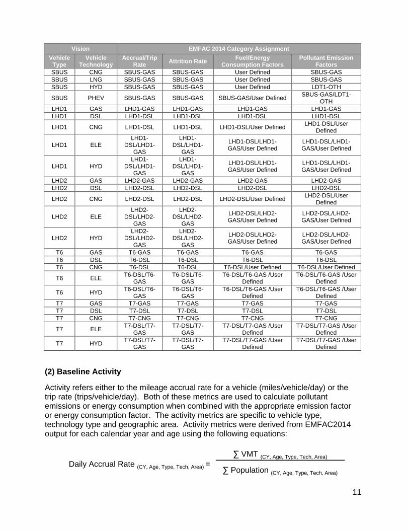
Both modules require inputs for population, activity, and emissions from EMFAC2014 from which attrition, sales, and emissions factors were derived. Because EMFAC2014 only provides output for certain vehicles technologies7 it was necessary to assign values to other vehicle/technology type combinations based on assumptions regarding similarities to the vehicle behaviors and engine technologies. As an example, Table 4 provides a summary of how the various vehicle/technology types found in EMFAC2014 were assigned to the vehicle/technology types represented in the modules. In the PVM module, variables for all eight technology types were assigned values while the variables in the HDV module were calculated and assigned on an as-needed basis.

(1) Baseline Attrition Rates

Attrition rates represent the survival fraction of vehicles of a particular age remaining in a fleet as the fleet ages. Attrition rates are specific to vehicle type, technology type and geographic area. Survival fractions were derived from EMFAC2014 output using the following equation:

Survival Fraction (CY, Age, Type, Tech, Area) = ∑ Population (CY, Age, Type, Tech, Area)

∑ Population (CY-1, Age-1, Type, Tech, Area)

7 In the case of electric vehicle technologies, EMFAC2014 only provides output for LDA and LDT1 vehicle types.

10

Table 4 EMFAC 2014 Vehicle Type and Technology Assignment Vision EMFAC 2014 Category Assignment

Vehicle Type

Vehicle Technology

Accrual/Trip Rate Attrition Rate Fuel/Energy

Consumption Factors Pollutant Emission

Factors LDA GAS LDA-GAS LDA-GAS LDA-GAS LDA-GAS LDA DSL LDA-DSL LDA-DSL LDA-DSL LDA-DSL LDA ELE LDA-OTH LDA-OTH User Defined LDA-OTH LDA ETH LDA-GAS LDA-GAS User Defined LDA-GAS LDA CNG LDA-GAS LDA-GAS User Defined LDA-GAS LDA LNG LDA-GAS LDA-GAS User Defined LDA-GAS LDA HYD LDA-OTH LDA-OTH User Defined LDA-OTH LDA PHEV LDA-GAS LDA-OTH LDA-GAS/User Defined LDA-GAS/LDA-OTH LDT1 GAS LDT1-GAS LDT1-GAS LDT1-GAS LDT1-GAS LDT1 DSL LDT1-DSL LDT1-DSL LDT1-DSL LDT1-DSL LDT1 ELE LDT1-OTH LDT1-OTH User Defined LDT1-OTH LDT1 ETH LDT1-GAS LDT1-GAS User Defined LDT1-GAS LDT1 CNG LDT1-GAS LDT1-GAS User Defined LDT1-GAS LDT1 LNG LDT1-GAS LDT1-GAS User Defined LDT1-GAS LDT1 HYD LDT1-OTH LDT1-OTH User Defined LDT1-OTH LDT1 PHEV LDT1-GAS LDT1-OTH LDT1-GAS/User Defined LDT1-GAS/LDT1-OTH LDT2 GAS LDT2-GAS LDT2-GAS LDT2-GAS LDT2-GAS LDT2 DSL LDT2-DSL LDT2-DSL LDT2-DSL LDT2-DSL LDT2 ELE LDT2-GAS LDT2-GAS User Defined LDT2-GAS LDT2 ETH LDT2-GAS LDT2-GAS User Defined LDT2-GAS LDT2 CNG LDT2-GAS LDT2-GAS User Defined LDT2-GAS LDT2 LNG LDT2-GAS LDT2-GAS User Defined LDT2-GAS LDT2 HYD LDT2-GAS LDT2-GAS User Defined LDT1-OTH LDT2 PHEV LDT2-GAS LDT2-GAS LDT2-GAS/User Defined LDT2-GAS/LDT1-OTH MDV GAS MDV-GAS MDV-GAS MDV-GAS MDV-GAS MDV DSL MDV-DSL MDV-DSL MDV-DSL MDV-DSL MDV ELE MDV-GAS MDV-GAS User Defined MDV-GAS MDV ETH MDV-GAS MDV-GAS User Defined MDV-GAS MDV CNG MDV-GAS MDV-GAS User Defined MDV-GAS MDV LNG MDV-GAS MDV-GAS User Defined MDV-GAS MDV HYD MDV-GAS MDV-GAS User Defined LDT1-OTH MDV PHEV MDV-GAS MDV-GAS MDV-GAS/User Defined MDV-GAS/LDT1-OTH

OBUS GAS OBUS-GAS OBUS-GAS OBUS-GAS OBUS-GAS OBUS DSL OBUS-DSL OBUS-DSL OBUS-DSL OBUS-DSL OBUS ELE OBUS-GAS OBUS-GAS User Defined OBUS-GAS OBUS ETH OBUS-GAS OBUS-GAS User Defined OBUS-GAS OBUS CNG OBUS-GAS OBUS-GAS User Defined OBUS-GAS OBUS LNG OBUS-GAS OBUS-GAS User Defined OBUS-GAS OBUS HYD OBUS-GAS OBUS-GAS User Defined LDT1-OTH

OBUS PHEV OBUS-GAS OBUS-GAS OBUS-GAS/User Defined OBUS-GAS/LDT1-OTH

UBUS GAS UBUS-GAS UBUS-GAS UBUS-GAS UBUS-GAS UBUS DSL UBUS-DSL UBUS-DSL UBUS-DSL UBUS-DSL UBUS ELE UBUS-GAS UBUS-GAS User Defined UBUS-GAS UBUS ETH UBUS-GAS UBUS-GAS User Defined UBUS-GAS UBUS CNG UBUS-NG UBUS-NG UBUS-NG UBUS-NG UBUS LNG UBUS-GAS UBUS-GAS User Defined UBUS-GAS UBUS HYD UBUS-GAS UBUS-GAS User Defined LDT1-OTH

UBUS PHEV UBUS-GAS UBUS-GAS UBUS-GAS/User Defined UBUS-GAS/LDT1-OTH

SBUS GAS SBUS-GAS SBUS-GAS SBUS-GAS SBUS-GAS SBUS DSL SBUS-DSL SBUS-DSL SBUS-DSL SBUS-DSL SBUS ELE SBUS-GAS SBUS-GAS User Defined SBUS-GAS SBUS ETH SBUS-GAS SBUS-GAS User Defined SBUS-GAS

11

Vision EMFAC 2014 Category Assignment Vehicle

Type Vehicle

Technology Accrual/Trip

Rate Attrition Rate Fuel/Energy Consumption Factors

Pollutant Emission Factors

SBUS CNG SBUS-GAS SBUS-GAS User Defined SBUS-GAS SBUS LNG SBUS-GAS SBUS-GAS User Defined SBUS-GAS SBUS HYD SBUS-GAS SBUS-GAS User Defined LDT1-OTH

SBUS PHEV SBUS-GAS SBUS-GAS SBUS-GAS/User Defined SBUS-GAS/LDT1-OTH

LHD1 GAS LHD1-GAS LHD1-GAS LHD1-GAS LHD1-GAS LHD1 DSL LHD1-DSL LHD1-DSL LHD1-DSL LHD1-DSL

LHD1 CNG LHD1-DSL LHD1-DSL LHD1-DSL/User Defined LHD1-DSL/User Defined

LHD1 ELE LHD1-

DSL/LHD1-GAS

LHD1-DSL/LHD1-

GAS

LHD1-DSL/LHD1-GAS/User Defined

LHD1-DSL/LHD1-GAS/User Defined

LHD1 HYD LHD1-

DSL/LHD1-GAS

LHD1-DSL/LHD1-

GAS

LHD1-DSL/LHD1-GAS/User Defined

LHD1-DSL/LHD1-GAS/User Defined

LHD2 GAS LHD2-GAS LHD2-GAS LHD2-GAS LHD2-GAS LHD2 DSL LHD2-DSL LHD2-DSL LHD2-DSL LHD2-DSL

LHD2 CNG LHD2-DSL LHD2-DSL LHD2-DSL/User Defined LHD2-DSL/User Defined

LHD2 ELE LHD2-

DSL/LHD2-GAS

LHD2-DSL/LHD2-

GAS

LHD2-DSL/LHD2-GAS/User Defined

LHD2-DSL/LHD2-GAS/User Defined

LHD2 HYD LHD2-

DSL/LHD2-GAS

LHD2-DSL/LHD2-

GAS

LHD2-DSL/LHD2-GAS/User Defined

LHD2-DSL/LHD2-GAS/User Defined

T6 GAS T6-GAS T6-GAS T6-GAS T6-GAS T6 DSL T6-DSL T6-DSL T6-DSL T6-DSL T6 CNG T6-DSL T6-DSL T6-DSL/User Defined T6-DSL/User Defined

T6 ELE T6-DSL/T6-GAS

T6-DSL/T6-GAS

T6-DSL/T6-GAS /User Defined

T6-DSL/T6-GAS /User Defined

T6 HYD T6-DSL/T6-GAS

T6-DSL/T6-GAS

T6-DSL/T6-GAS /User Defined

T6-DSL/T6-GAS /User Defined

T7 GAS T7-GAS T7-GAS T7-GAS T7-GAS T7 DSL T7-DSL T7-DSL T7-DSL T7-DSL T7 CNG T7-CNG T7-CNG T7-CNG T7-CNG

T7 ELE T7-DSL/T7-GAS

T7-DSL/T7-GAS

T7-DSL/T7-GAS /User Defined

T7-DSL/T7-GAS /User Defined

T7 HYD T7-DSL/T7-GAS

T7-DSL/T7-GAS

T7-DSL/T7-GAS /User Defined

T7-DSL/T7-GAS /User Defined

(2) Baseline Activity

Activity refers either to the mileage accrual rate for a vehicle (miles/vehicle/day) or the trip rate (trips/vehicle/day). Both of these metrics are used to calculate pollutant emissions or energy consumption when combined with the appropriate emission factor or energy consumption factor. The activity metrics are specific to vehicle type, technology type and geographic area. Activity metrics were derived from EMFAC2014 output for each calendar year and age using the following equations:

Daily Accrual Rate (CY, Age, Type, Tech, Area) = ∑ VMT (CY, Age, Type, Tech, Area)

∑ Population (CY, Age, Type, Tech, Area)

12

Daily Trip Rate (CY, Age, Type, Tech, Area) = ∑ Trips (CY, Age, Type, Tech, Area)

∑ Population (CY, Age, Type, Tech, Area) (3) Baseline Emission Factors

Emission factors represent the mass of pollutant emitted per unit of activity. As with attrition rates and activity metrics, emission factors are specific to vehicle type, technology type and geographic area. Emission factors are further subdivided into various emissions processes. Exhaust processes such as start, running and idle emit all the pollutants reported while brake wear and tire wear only generate particulates (PM, PM10 and PM2.5). Evaporative processes, like running loss emissions, hot soak emissions, resting loss emissions and diurnal, are significant contributor of hydrocarbon emissions (HC, ROG, and TOG). Based on practical needs and engineering judgment, several of the processes were combined to create overall emission factors in the PVM module. Table 5 provides a summary of the calculations required to estimate the emission factors for each of the pollutant and process combinations.

Table 5 Baseline Emission Factor Calculations

Process

EMFAC2014 Output Calculations

PVM HDV

Activity Used EF Units Activity Used EF Units

Start Trip tons/trip VMT tons/mile

Running VMT (combined running and idle

emissions as running emissions)

tons/mile VMT tons/mile

Idle VMT tons/mile

Brake Wear VMT tons/mile VMT tons/mile

Tire Wear VMT tons/mile VMT tons/mile

Running Loss Trip (combined running loss and hot soak

emissions as running loss emissions)

tons/trip VMT tons/mile

Hot Soak VMT tons/mile

Resting Loss Vehicle (combined

resting loss and diurnal emissions as

resting loss emissions)

tons/vehicle VMT tons/mile

Diurnal VMT tons/mile

*Emission factors are function of calendar year (CY), age, vehicle type, technology and area

13

(4) Baseline Fuel Efficiency

Table 6 provides a summary of the calculations required to estimate fuel efficiencies for start, running and idle processes from EMFAC output. Fuel efficiencies for alternative fuel vehicles in the PVM are expressed in units of miles per gasoline gallon equivalent (mpgge). Fuel efficiencies for non-gasoline and non-diesel technologies are derived from the National Academy of Sciences study on “Transitions to Alternative Vehicles and Fuels (NRC 2013)” and assigned to the various other technology types found in the PVM and discussed in Appendix B. In the HDV module, base fuel type (fuel type in baseline scenario) determines the fuel equivalency. For vehicle categories with gasoline as base fuel, the fuel economy units are expressed in gasoline gallon equivalent. All other vehicles in the HDV module are in diesel gallon equivalent. The fuel/energy economies for heavy duty zero emission technologies are assumed to be 58% more efficient than conventional combustion technologies, within the Energy Economy Ratio ranges assumed in LCFS8.

Table 6 Baseline Fuel Economy Calculations

Process EMFAC2014 Output Calculations

PVM HDV

Start Trips/gallon = (trips/day)/(start fuel consumption/day)

Miles/gallon = (miles/day)/(start fuel consumption/day)

Running Miles/gallon = (miles/day)/(running and idle fuel consumption/day)

Miles/gallon = (miles/day)/(running fuel consumption/day)

Idle Miles/gallon = (miles/day)/(idle fuel consumption/day)

(5) Baseline Sales Fractions

The sales fractions for the various technology types found in the on-road modules are specific to vehicle type, technology type and geographic area. The sales fractions in PVM module for a given calendar year were determined based on the number of “Age 0” vehicles in a given calendar year and calculated using the following equation:

Sales Fraction (CY, Age, Type, Tech, Area) in PVM

= ∑ Population (CY, Age(0), Type, Tech, Area)

∑ Population (CY, Type, Tech, Area)

In the HDV module, the sales for a given calendar year were determined based on the number of vehicles in the module of a specific model year, compared to the year prior. This was then divided by the total vehicle purchases with a vehicle type and technology to

8 The LCFS Credit Price Calculator, http://www.arb.ca.gov/fuels/lcfs/dashboard/creditpricecalculator.xlsx

14

determine sales fraction within a year, as shown in the following equation:

Sales Fraction (CY, Age, Type, Tech, Area) in HDV

= ∑ Population (CY, Age, Type, Tech, Area) - ∑ Population (CY-1, Age-1, Type, Tech, Area)

∑ Vehicle Purchases (CY, Age, Type, Tech, Area)

(6) Additional Modifications to EMFAC2014 Data

In addition to the extra steps described earlier to generate the special EMFAC output, more modifications were necessary to create the final baseline used as the starting point for evaluation of all other Vision scenarios, as listed below.

PVM modifications:

• Splitting total ZEV sales between LDA and LDT2 vehicle categories. EMFAC2014 apportions all ZEV sales resulting from the Advanced Clean Cars regulation to LDAs only. For the VISION baseline, total ZEV sales from the EMFAC2014 model were split between LDA and LDT vehicles. The sales fraction splits begin in 2016 and reflect a greater proportion of ZEV sales being allocated to the LDT2 category. Specifically, 0% of ZEV are allocated to LDT2s in 2015 but gradually increase to 20%, 33% and 25% in 2025 for BEVs, FCEVs, and PHEVs, respectively.

• Accrual and trip rate reductions to LDA and LDT2 BEVs for model years 2010 to 2025. These reductions reflect the reduced range of BEVs for these model years relative to gasoline-powered vehicles. Specifically, the accrual rate for an LDA/LDT2 BEV is 50% of an LDA/LDT2 gasoline vehicle for model year 2010. The accrual rate for each successive model year increases gradually until model year 2025 whereby the accrual rate for BEV and gasoline vehicles are equivalent. In order to keep the total VMT constant for the LDA and LDT2 sector, the accrual rates for gasoline vehicles were increased by an adjustment factor each calendar year to account for the reduced BEV VMT. The magnitude of the adjustment factors ranged from 0.0 to 0.3%.

• eVMT degradation for PHEVs. The EMFAC2014 model assumes the eVMT fraction of total VMT travelled by PHEVs is constant (i.e. 40%) throughout the life of the vehicle. For the VISION baseline, staff assumed there was degradation in the eVMT fraction of total VMT travelled by PHEVs such that the eVMT fraction decreases over the life of the vehicle. Specifically, the eVMT fraction decreases with age such that the eVMT fraction is only 90% of new vehicle (i.e. age 0) eVMT fraction by the time the vehicle reaches age 15. The Cleaner Fuels and Technology scenario discussed below explores the impact of the expanded eVMT.

• eStart fraction for PHEVs. The EMFAC2014 model assumes the eStart fraction (i.e. the number of starts in electric mode) for PHEVs is constant (i.e. 40%). For the VISION 2.0 baseline, staff assumed the eStart fraction to be 20% throughout the life of the vehicle. In VISION 2.1 Scenario 2 the eStart fraction and eVMT fraction maintain a 1:2 ratio throughout the vehicle life time.

• Increased fuel efficiency in PHEVs. The fuel efficiency of PHEVs while operating in combustion mode is increased by 25% to account for the advanced design and fuel

15

efficiency of the engines in these vehicle types.

Scenario Assumptions:

The scenarios included in this version of the PVM and HDV modules relied on both the baseline data and a series of assumptions about the technologies and implementation, which are documented below. For heavy duty vehicles, the assumptions for the SIP Measures and Cleaner Technologies and Fuels scenarios are the same. The expanded zero emission technology scenario, which assumes higher zero emission technology penetrations in the heavy duty sector discussed in the 2016 Mobile Source Strategy4

, is also included in the following description.

Baseline/Current Control Programs

PVM

• Advanced Clean Car: ARB’s emissions-control program for light duty passenger vehicles model years 2017 through 2025 adopted in 2012. The program combines the control of smog, soot and global warming gases and requirements for greater numbers of zero-emission vehicles.

• SB375: The Sustainable Communities Act supports the State's climate action goals to reduce greenhouse gas (GHG) emissions through coordinated transportation and land use planning with the goal of more sustainable communities.

HDV

• GHG Phase I: US EPA’s measure to improve fuel efficiency and reduce green-house gas emissions from model years 2014~2018 heavy duty trucks.

• ARB Tractor-Trailer Regulation: requires the use of aerodynamic tractors and trailers to reduce GHG emissions.

• ARB Truck and Bus Rule: ARB’s measure to accelerate turnover of heavy duty trucks to the on-road 2010 emission standard by 2023.

• ARB Drayage Truck Regulation: Requires drayage trucks in South Coast to upgrade to 2007 or newer engines, with 2010 or newer required in 2023.

• ARB Public Fleets Rule and Solid Waste Collection Vehicle Rule: Fleets must apply the Best Available Control Technology (BACT) to reduce PM emissions, with multiple options depending on the truck model year.

SIP Measure Concepts

PVM

• Assumed combined LDA/LDT2 ZEV/PHEV sales increase from 18 percent to 40 percent between 2025 and 2030.

• Assumed MDV ZEV/PHEV sales beginning in 2025, ramping up to 10 percent by 2030.

• Assumed increased fuel efficiency (~2.9 percent per year) 2025 to 2035 for gasoline vehicles.

16

• Assumed new SULEV NOx standard phased in between 2025 and 2030 for gasoline LDAs. 100 percent SULEV20 sales by 2030

• Assumed Urban Bus ZEV sales, both battery and fuel cell technologies, begin in 2018 and increase to 100 percent of all sales in 2030

• Assumed 100 percent purchases of Low-NOx standard starting model years 2018 and 2020 for natural gas and diesel buses, respectively

HDV

• Federal Low-NOx Engine Standards Combining the Low-NOx Engine Standards and Lower In-Use Emission Performance Level measures, staff applied a flat 90 percent reduction in NOx emissions from the current 2010 standard for all exhaust processes throughout the life of the vehicle. For modeling purpose, staff assumed 100% of model year 2024 and newer trucks will be impacted by the measure. The splits between and natural gas depended on technology availability, vocation and infrastructure. Long-haul trucks would still be dominated by low-NOx while local delivery trucks were assumed to have higher penetration of natural gas low-NOx.

• California Only Low-NOx Engine Standards This measure is similar to Federal Low-NOx Engine Standards but would only impact vehicles purchased new in California. Since significantly more used federal standard trucks will migrate to California than used trucks meeting California standard migrating out, the benefit of California only Standard would be a fraction of the reduction achieved with Federal Standards. Staff used simplified purchase fractions and derived survival rates to simulate the overall impact of California Only Low-NOx Standard.

• Medium and Heavy-Duty Greenhouse Gas Phase 2 Reductions in CO2 and fuel consumptions phase in from 2018 to 2027 with 5 to 25 percent efficiency improvements depending on vocation beyond currently adopted GHG Phase I and ARB’s Tractor-Trailer Regulation.

• Last Mile Delivery (LMD) Staff identified several local Class 3 to 7 vehicle categories in EMFAC2014 that are most likely to include fleets impacted by this measure. Based on projected heavy duty ZEV population for the measure, staff assumed 2.5 percent of new sales starting 2020 to be battery or fuel cell technologies. The zero emission technology penetration ramping up to 10 percent by 2025 and remain flat thereafter. The actual last mile delivery fleets would be a subset of these categories and the percent sales assumptions were applied equally to the categories identified.

Cleaner Technologies and Fuels

PVM

• Assumed combined LDA/LDT2 ZEV/PHEV sales increase from 18 percent to 40 percent between 2025 and 2030, and reach 100 percent by 2050.

• Assumed MDV ZEV/PHEV sales beginning in 2025, ramping up to 10 percent by

17

2030, and reach 50 percent by 2050. • Assumed increased fuel efficiency (~2.9 percent per year) for gasoline vehicles

starting 2025. • Assumed new SULEV NOx standard phased in between 2025 and 2030 for gasoline

LDAs. 100 percent SULEV20 sales by 2030. • Assumed VMT reductions ramping up to 15 percent below 2050 baseline VMT in

2050. • Assumed extended electric range for PHEVs after 2025 from 40 percent to 60

percent eVMT by 2050.

HDV – same as SIP Measure Concepts

Expanded Zero-Emission for HDV

This scenario reflected expansion of zero emission technologies beyond those assumed in the Cleaner Technologies and Fuels scenario. • Assumed same ZEV penetration as in the SIP Measures scenario until 2025; the

penetration rate increases beyond 2025, from 10% in 2025 to 35% in 2050 for the local Class 3 to 7 trucks identified in Last Mile Delivery Measure assumption

• Since there is no SIP Measure requirement, the penetration of zero emission technologies for the remaining instate Class 2B~6 trucks was assumed to have a 3-year lag behind that of local Class 3 to 7 in LMD

• The zero emission port truck demonstration program will accelerate the technology penetration for drayage trucks serving in South Coast and the zero emission truck population in the fleet could reach 3,000 in 2033

• From 2030 on, sales of zero emission vehicle in other instate Class 7 and 8 would begin, growing to 10 percent by 2050

18

Off-Road Vision Module for Forklifts And Airport Ground Support Equipment The Vision 2.1 Off-Road Vision module builds off of ARB’s official off-road inventories for In-Use Off-Road Equipment and OFFROAD20079 which contains the Large Spark-Ignited (LSI) Equipment Regulation10 categories. The Off-Road module forecasts populations, activity, fuel consumption and pollutant emissions for forklifts and airport ground support equipment (GSE). All forecasts are provided out to calendar year 2050. There have been no changes to the Off-Road Vision module since the October 2015 release of Vision. Baseline Emissions Inventory Assumptions:

The Off-Road Vision module was developed relying heavily on the methodology and output from ARB’s official off-road emissions inventory models: OFFROAD2007 for spark ignition equipment; 2010 In-Use Off-Road Emissions Inventory (2010 In-Use) and associated Off-road Simulation Model (OSM) for diesel equipment. The outputs from these three official off-road models serve as baseline for Off-Road Vision, and include information equipment class, type and rating; fuel type and consumption; activity; vehicle population; model and calendar years, geographic location, and pollutant emissions. The module’s inventory assumptions such as turnover, activity, sector growth, regional allocation, etc. are also inherited by the fundamental methodologies behind these models. Detailed information on these models is available at: http://www.arb.ca.gov/msei/categories.htm#offroad_motor_vehicles. Off-Road Vision Module Scenario Assumptions:

Scenarios in the Off-Road Vision module are evaluated through vehicle sales by model year, technology type, and vehicle type. Specifically, this is accomplished by scaling model year output for vehicle types targeted by the proposed measures. The module adjusts the output from these models by selecting the emissions from vehicles targeted and setting their emissions to zero simulating the replacement of a combustion engine with an electric engine.

The “SIP Measure Concepts” scenario in the Strategy document models deployment of zero emission vehicle technologies into targeted equipment categories such as forklifts and airport ground support equipment.

• Zero Emission Off-Road Forklift Regulation Phase 1: This measure considers electrification of small forklifts (less than 65 horsepower) in the industrial and airport ground support sectors through incentives as well as natural and accelerated turnover. Approximately 73% of forklifts in California were determined to be in medium or large fleets, and it was assumed that 90% of qualifying forklifts (aggregate 67.5%) could reasonably be targeted for electrification by 2035 with the electrification starting in 2028. A linear penetration of replaced equipment to

9 Mobile Source Emissions Inventory http://www.arb.ca.gov/msei/categories.htm 10 Off-road Large Spark Ignition Equipment Regulation, http://www.arb.ca.gov/msprog/offroad/orspark/orspark.htm

19

2035 was applied to the output data from the three official off-road models mentioned above.

• Zero Emission Airport Ground Support Equipment: This measure considers electrification of certain airport ground support equipment (belt loaders, baggage tugs, and cargo tractors) through incentives and natural turnover. Using the turnover inherent in the official OSM model, all new vehicles of these types will be electric starting in 2023. Natural turnover is allowed to accomplish the replacement of the GSEs, meaning equipment that would have been purchased at the normal rate in the future would simply be electric instead of with no acceleration of purchasing habits.

20

Ocean Going Vessel (OGV) Module The Vision 2.1 Ocean Going Vessel (OGV) module forecasts energy consumption, activity, and pollutant emissions of commercial vessels that are either at least 10,000 gross tons or 400 feet in length in California waters under various SIP compliance strategies.

The OGV module output is specific to three different geographic domains. The first is a statewide domain consisting of the entire coastline. The second and third are the South Coast Air Basin (SCAB) and the San Joaquin Valley Air Basin (SJVAB) consisting of the counties and geographic areas defined by California Law for those air basins. Statewide forecast are provided out to 2050, while the San Joaquin Valley and South Coast forecasts are provided out to calendar year 2030.These three domains have two different outer boundaries over the ocean that are used in the module. The first zone is within 24 nautical miles of the California coastline that is defined in California law and is also used for regulatory purposes. The second zone is within 100 nautical miles of California’s mainland coastline.

The baseline inputs and scenario assumptions in the Vision OGV module are the same as those in Vision 2.0. Staff did, however, refine and enhance model structure such that the calculations and outputs are easier to follow. Baseline Emissions Inventory Assumptions:

The OGV module relies on an early draft of the Marine Emissions Model (MEM) version 2-3L11 for the modules baseline input data. Data generated from the MEM was further processed to derive baseline input data in a format compatible with the OGV module. The MEM outputs for activity, fuel use and pollutant emissions were aggregated by operational mode, calendar year, and geographic domain. There are four operational modes that characterize vessel activity: transiting (traveling at open sea), maneuvering (slow speed operations while in a port), hoteling (moored to a dock) and anchorage (moored by anchor).

The OGV module also includes data that are not obtained from the MEM. Marine energy consumption from the MEM only specifies if residual oil or fuel was used, and does not account for electricity consumption from shorepower. Therefore, the OGV module estimated the amount of electricity consumed by vessels utilizing shorepower. The OGV module also requires turnover rates of the vessels. The MEM provides a turnover rate based on the vessel type. For the purposes of the OGV module, a weighted average of the turnover was calculated.

The MEM does not include, at this time, the Energy Efficiency Design Index (EEDI) that came into effect in 2015. This regulation was passed by the International Maritime Organization and requires that new vessels be 10% more fuel efficient beginning 2015, 20% more efficient beginning 2020, and 30% more efficient beginning 2025. Instead, the

11 OGV Model Version 2-3L https://www.arb.ca.gov/msei/categories.htm#offroad_motor_vehicles

21

baseline module inputs are based on IMO’s 2014 Greenhouse Gas study12. Ocean Going Vessels Module SIP Measure Assumptions:

At-Berth Regulation Amendments: This measure requires that additional vessels (i.e., auto carriers, bulk cargo, general cargo, roll-on roll-off carriers, and tankers) would connect to shore power rather than run auxiliary engines. For modeling purposes, the amendments were limited to the ports that are currently offering shore power and implementation was assumed to start in 2022 at 10 percent fleet compliance and to increase to 50 percent fleet compliance by 2032. This compliance rate was converted into the number of ships impacted, and then multiplied by the average time spent at berth. As the current regulation allows between three to five hours of auxiliary engine operation for each affected visit, four hours was used as the average time spent at berth using auxiliary engines. The results from above were then combined to find the total hours of auxiliary engine use at berth that would be reduced by the amendments. Tier IV Vessel Standards: The measure would require that 100 percent of new vessels meet Tier 4 NOx emissions standards, starting in the calendar year 2025. Tier 4 NOx emission standards are 70 percent lower than existing Tier 3 standards. The new standards would be allowed to enter the fleet using natural turnover and would not be accelerated by additional rules or incentives.

12 Third IMO Greenhouse Gas Study: http://www.imo.org/en/OurWork/Environment/PollutionPrevention/AirPollution/Documents/Third%20Greenhouse%20Gas%20Study/GHG3%20Executive%20Summary%20and%20Report.pdf

22

Line Haul Locomotives Module The Vision 2.1 Locomotive model uses as a starting point the most current locomotive inventory, which was updated in 201413. This inventory is one of the most comprehensive assessments of locomotive operations in California. The Vision Locomotive module builds off this inventory and forecasts fuel consumption and emissions for line-haul locomotives out to calendar year 2050. The Locomotive module output is provided for eleven of the fifteen defined air basins in California, which include Mountain Counties (MC), Mojave Desert (MD), North Central Coast (NCC), Northeast Plateau (NEP), South Coast (SC), South Central Coast (SCC), San Diego (SD), San Francisco Bay Area (SF), San Joaquin Valley (SJV), Salton Sea (SS), and Sacramento Valley (SV). Data is not provided for Great Basin Valleys, Lake County, Lake Tahoe, and the North Coast as line-haul rail activity data is not present in those air basins. Baseline Emissions Inventory Assumptions:

The Vision Locomotive module uses the official locomotive inventory13 as the initial input into the module. This inventory was developed using activity data provided by the rail lines, which included activity (duty cycle and gross ton-miles), fuel consumption, and Tier distribution data, and combined with locomotive Tier emissions data provided by the US EPA’s Non-road engines and Vehicles Emissions Standards inventory14. ARB then allocated those data across county, air district, and air basin, and uses this allocation as the base data going forward. The growth rate is calculated from other ARB inventory models or external industry data. The Vision module’s inventory assumptions are directly inherited by the fundamental methodologies behind the official locomotive inventory. Locomotive Vision Module Scenario Assumptions:

More Stringent National Locomotive Emissions Standards: Newly manufactured locomotives: The Tier 5 emissions standard was modeled as a new tier of locomotives to be introduced in 2025. Tier 5 is defined by the same emission standards as Tier 4 for all pollutants except NOx, and PM, for which the standard is 75% lower for NOx and 67% lower for PM. This was represented in the model by increasing the Tier 5 locomotive population in the total tier distribution by ~4.0 percent per year over the baseline population with an equal reduction in the Tier 4 distribution. Remanufactured Locomotives: Remanufactured locomotives: The locomotive fleet meeting the remanufacture emissions levels is modeled such that 95 percent of line-haul locomotive activity is represented by Tier 4 locomotives by 2031, with phase-in of Tier 4 starting in 2023. For modeling purposes, this is represented by increasing the Tier 4 locomotive population in the total

13 Locomotive Emission Inventory: http://www.arb.ca.gov/msei/goods_movement_emission_inventory_line_haul_octworkshop_v3.pdf 14 US EPA Non-Road Engines and Vehicles Emissions Standards: https://www.epa.gov/emission-standards-reference-guide/nonroad-engines-and-vehicles-emission-standards

23

tier distribution by ~8 percent per year over the baseline with an equal total reduction in the lower tier populations to account for the increase in Tier 4.

24

Energy Module (EM) The Vision 2.1 energy module is used to evaluate the liquid fuels, electric power, hydrogen, and natural gas required to supply the demands of the demand models. Additionally, the energy module calculates the upstream WTT emissions associated with fuel consumption and total WTW greenhouse gases based on the composition of the fuels used in the scenario. The module processes energy demand and tailpipe emissions output data from the demand modules (e.g. PVM, HDV, OGV, rail, etc), with assumptions about fuel blending, supply capacities and emission factors. The module then estimates consumed quantities of finished fuels, feedstocks, electricity, and other supplies required to meet demand module energy requirements and their associated emissions. Upstream emissions in the EM cover the direct emissions resulting from the process required to producing, refining and delivering the energy requirements (also referred to as well-to-tank (WTT or WtT). Emissions coming from the demand sectors, also referred to as tank-to-wheel (TTW or TtW) emissions, comes from the transportation sector modules directly, and are combined with the WTT emissions calculated in the EM for a full well-to-wheel (WTW) assessment.

The EM contains six demand sectors: passenger vehicle module (PVM), heavy duty vehicle (HDV) module, locomotive, ocean going vessels (OGV), off-road equipment (forklift and ground support), and Other. The Other sector contains air, construction and agricultural vehicles. It also contains other non-demand sectors like high global warming potential emissions, non-combustion agricultural emissions and waste processing emissions.

25

Demands from the various sectors are bundled into the following fuel types:

EM Fuel Bundle Description GAS Gasoline DSL Diesel

DSL_US_C Imported Conventional Diesel O85 85% Blend Ethanol NG Natural Gas (pipeline)

CNG Compressed Natural Gas LNG Liquefied Natural Gas ELE Grid Electricity HYD Hydrogen JET Jet Fuel

The energy module contains a number of different fuels and blend stocks, including:

Table 7: Vision Fuels and Blend stocks

Demand Blend stocks

Gasoline CARBOB, Ethanol, Renewable Gasoline Diesel ULSD, Bio-diesel, Renewable diesel

Electricity Coal, Natural Gas, Nuclear, Hydro, Natural gas Fossil, Landfill, AD Gas

Hydrogen Reformed Natural Gas, Biomass, Wind, Jet Fuel Petroleum, Bio-Jet, Renewable Jet

Model Inputs and Constraints:

(1) Emission Factors An ARB internal analysis was performed to calculate California specific statewide average emission factors for upstream fuel production. Criteria pollutant emission factors were derived from several data sources: • CA-specific facility emissions (CEIDARS15) • CA-specific fuel production throughputs/capacities (CEC16, DOGGR17, EIA18, DOE19) • CAGREETv220 national averages for fuels not currently produced in CA

15 District Resources for Emission Inventory - Database References - http://www.arb.ca.gov/ei/drei/maintain/database.htm 16 2012 Weekly Fuels Watch Report - http://energyalmanac.ca.gov/petroleum/fuels_watch/reports/2012_Weekly_Fuels_Watch_RPT.xls 17 Department of Conservation's Division of Oil, Gas, and Geothermal Resources - http://www.conservation.ca.gov/dog 18 U.S. Energy Information Administration - http://www.eia.gov/ 19 Hydrogen Analysis Resource Center - http://hydrogen.pnl.gov/ 20 CA-GREET 2.0 Model and Documentation - http://www.arb.ca.gov/fuels/lcfs/ca-greet/ca-greet.htm

26

For the fuels that are not produced in California, a scalar was applied to reflect the differences between average California refineries in comparison to a national refinery (conventional fuel production). GHG emission factors were derived from: • CA GHG emissions Inventory21 • CA-specific fuel production throughputs/capacities (CEC22, DOGGR23, EIA24, DOE25) • CAGREETv226 national averages for fuels not currently produced in CA

(2) Energy Module Supply Constraints

Petroleum Fuels The supply curves placed on petroleum fuels do not actually constrain the usage of fossil fuels. The constraint is used primarily for the purposes of calculating the quantity of finished fuels that will be exported to external markets. It is assumed that the quantity of finished petroleum fuels produced in California in 2012 is indicative of the capacity for California’s refiners. The 2012 production data was provided by the CEC, based upon the CEC’s Weekly Fuels Watch Report27. Renewable Natural Gas The other major supply constraint provided in the Vision model is on Renewable Natural Gas. The technical potential of Renewable Natural Gas is informed by ARB’s Proposed Short-Lived Climate Pollutant Reduction Strategy28 (SLCP). The Baseline or Current Control scenario assumes a negligible amount of renewable natural gas production from landfills and dairy sources. The SIP and CTF scenarios have a modest increase renewable natural gas produced from dairy and landfill sources. DOE 2011 Billion Ton Study Update Biofuel consumption is generally unconstrained within the EM. A broad analysis of the DOE’s 2011 Billion Ton Study Update 29was performed to analyze biofuel/feedstocks that could potentially flow to California to help it meet its climate change goals. It was determined that a realistic capacity for biofuels in California to be on the approximately 6.5 billion gallons gasoline equivalent. All scenario runs are compared to this number to ensure estimated biofuel consumption doesn’t exceed this capacity.

21 California Greenhouse Gas Emission Inventory Program - http://www.arb.ca.gov/cc/inventory/inventory.htm 22 2012 Weekly Fuels Watch Report - http://energyalmanac.ca.gov/petroleum/fuels_watch/reports/2012_Weekly_Fuels_Watch_RPT.xls 23 Department of Conservation's Division of Oil, Gas, and Geothermal Resources - http://www.conservation.ca.gov/dog 24 U.S. Energy Information Administration - http://www.eia.gov/ 25 Hydrogen Analysis Resource Center - http://hydrogen.pnl.gov/ 26 CA-GREET 2.0 Model and Documentation - http://www.arb.ca.gov/fuels/lcfs/ca-greet/ca-greet.htm 27 2012 Weekly Fuels Watch Report - http://energyalmanac.ca.gov/petroleum/fuels_watch/reports/2012_Weekly_Fuels_Watch_RPT.xls 28 SLCP Proposed Strategy - https://www.arb.ca.gov/cc/shortlived/shortlived.htm 29 U.S Department of Energy Billion Ton Study 2011 Update - https://bioenergykdf.net/content/billiontonupdate

27

(3) Scope, Nodes and Conversion Factors

There are two main Scopes used by the EM: 1. CA – Emissions and processes that occur within the AB32 boundary 2. US – Emissions and processes that occur externally to the AB32 boundary. Although

labeled US, this process may occur Internationally.

The nodes utilized by the EM characterize steps a feedstock travels from production to being placed within a fuel tank. For example, the nodes utilized by CARBOB are:

1. Production field (where the crude oil is produced) 2. Refinery 3. Bulk Terminal

While the nodes ethanol travel in the real world may have additional steps, this process was simplified in this version of Vision.

The EM uses CAGREETv2 as a reference for all conversion factors for conversions between volume and energy content. The lower heating value is typically used. (4) Energy Module Blending

The EM uses the blending table to determine what components (if any) are used to produce the resources being analyzed. There are two main methodologies that the EM uses to determine component quantities.

1. Arbitrary blending Arbitrary blending is used when a fixed ratio of blending is required. The EM prioritizes the analysis of each arbitrary component first, and verifies there is adequate supply to meet the demand. Recursion into these components occurs before any optimized blend stocks are analyzed. If the supply functions of the EM cannot provide enough resources to meet the component’s demand, and error occurs and the module terminates.

2. Optimized blending After the EM fulfills the demands required for the arbitrary components; the EM evaluates any components that are to be optimized. The rank field provides the means for the EM to perform the prioritization of possible components.

In this release, each component uses a 4-digit ranking number. The first digit is dedicated to the scope of the node this resource is associated with. This allows the EM to choose pathways that are local before choosing external sources. The second digit is an indicator of three main types of resources: (1) renewable, (2) biomass derived or (3) conventional. The optimization then looks to how clean a pathway is for prioritization. The last two digits are ranking on similar fuel, typically referencing Carbon Intensity (CI) of pathways according to CAGREETv2.

Appendix C provides detailed descriptions on Energy Module project processing.

28

Scenario Assumptions:

The baseline or Current Control Program scenario reflects all adopted and implemented policies. The Cleaner Technology and Fuels (CTF) scenario explored a path to getting deeper NOx reductions and identifying a potential pathway to meeting climate goals. The SIP Measure Concept case was designed to reflect ARB’s policy concepts to attain the 2008 Federal Ozone Air Quality Standards.

Baseline/Current Control Programs

• Blend assumptions for liquid fuels in the transportation sector come from the Low Carbon Fuel Standard (LCFS) Regulation. Appendix B of LCFS’s ISOR30 contains an illustrative scenario for compliance. This compliance curve is used to calibrate the baseline scenario.

• Phase 3 California Reformulated Gasoline Regulations (RFG3)31 provides the maximum oxygenate content for CARFG, which is 10% by volume. All scenarios do not exceed this blend wall.

• ASTM D97532 provides a similar blend wall for diesel fuel. This places a maximum blend of biodiesel at 5%. All scenarios do not exceed this 5% blend wall for biodiesel.

• The base assumption for electric power generation blends is the Renewable Portfolio Standard (RPS). Pursuant to SB1078, SB107, and SB2, the RPS requires investor-owned utilities (IOUs), electric service providers, and community choice aggregators to increase procurement from eligible renewable energy resources to 33% of total procurement by 2020. All scenarios use this standard as a foundation for electric power generation blends.

• The Emission Performance Standards33, pursuant to SB1368, limits long-term investments in baseload generation by the state's utilities to power plants that meet an emissions performance standard (EPS) jointly established by the California Energy Commission and the California Public Utilities Commission. SB1368 effectively bans new contracts from coal power generators. The CEC projects34 coal will phase out in 2027-2028.

• The San Onofre Nuclear Generation Station (SONGS) was retired in 2013. It is assumed that additional natural gas baseload power generators were used to displace the nuclear power SONGS produced.

• The Diablo Canyon Power Plant (DCPP) is the only remaining nuclear power generation facility in California. In the baseline it is assumed that the DCPP will be relicensed and will continue to generate its current capacity.

30 Low Carbon Fuel Standard Regulation - http://www.arb.ca.gov/regact/2015/lcfs2015/lcfs2015.htm 31 Phase 3 California Reformulated Gasoline Regulations - http://www.arb.ca.gov/regact/2007/carfg07/carfg07.htm 32 Standard Specification for Diesel Fuel Oils - http://www.astm.org/Standards/D975.htm 33 Emission Performance Standard - http://www.energy.ca.gov/emission_standards/index.html 34 Current expected energy from coal - http://www.energy.ca.gov/renewables/tracking_progress/documents/current_expected_energy_from_coal.pdf

29

• The CEC released an analysis35 of future effects of climate change on California’s generated, and procured, hydropower generation. All scenarios displace hydropower and with natural gas production to make up for reduced hydropower generation.

• SB150536 regulates the renewable content of transportation hydrogen. The regulation will require providers of hydrogen to produce 33.3 percent of the hydrogen from eligible renewable energy resources. It is assumed this percentage will be reached in 2020, when SB1505 is expected to go into effect.

• Based in part on the Short Lived Climate Pollutant Plan (SLCP), 10% of the technical potential of renewable natural gas is used to supply demand.

SIP Measure Scenario

• Assumed 50 percent of the diesel pool is renewable by 2030. Assumes an overall ~14 percent reduction in diesel carbon intensity.

• DCPP will not be relicensed, and displaces the nuclear power with additional natural gas baseload generation.

Cleaner Technology and Fuels Scenario

• In the 2013 Scoping Plan Update37, a strategy to extend LCFS was discussed. The SMC and CTF scenarios both use an expanded LCFS target of 18% CI reduction in 2030 as a foundation for blending fuels.

• In 2015, the signing of SB350 further expands RPS to increase procurement of renewable energy resources to 50% of the total procurement by 2030.

• There is an inclusion of renewable jet fuel to a blend of 5% by 2020. • All proposed methane reductions from the SLCP will be redirected towards

renewable natural gas supply. • A linear growth of in-state produced biofuels from 25% in 2020 to 100% in 2050. • A linear expansion of renewable hydrogen from 33% in 2025 to 75% in 2050.

35 Potential Changes in Hydropower Production from Global Climate Change in California and the Western United States - http://www.energy.ca.gov/2005publications/CEC-700-2005-010/CEC-700-2005-010.PDF 36 Environmental & Energy Standards for Hydrogen Production - http://www.arb.ca.gov/msprog/hydprod/hydprod.htm 37 First Update to the AB 32 Scoping Plan - http://www.arb.ca.gov/cc/scopingplan/document/updatedscopingplan2013.htm

30

Appendix A: Current Control Measures Included in the Vision Model

Biofuels:

Low Carbon Fuel Standard • Pursuant to AB32 and S-01-07 • Requiring the Carbon Intensity of transportation fuels to be reduced by 10% in 2020

from a 2010 baseline. • Dec 30, 2014 - Staff Report - Initial Statement of Reasons - Appendix B:

Development of Illustrative Compliance Scenarios and Evaluation of Potential Compliance Curves http://www.arb.ca.gov/regact/2015/lcfs2015/lcfs15appb.pdf

Renewable Fuel Standard • Pursuant to the Energy Policy Act (EPAct) of 2005 and Security Act (EISA) of 2007 • Requires a varying amount of biofuels to be mixed into Gasoline and Diesel

http://www3.epa.gov/otaq/fuels/renewablefuels/documents/420f15028.pdf

California production of Biofuels, S-06-06 • Requires the state to produce a minimum of 20 percent of its biofuels within California

by 2010, 40 percent by 2020, and 75 percent by 2050 http://www.arb.ca.gov/fuels/altfuels/incentives/eos0606.pdf

SB350 - 50% RPS • Raises California’s renewable portfolio standard from 33% to 50% by 2030

http://focus.senate.ca.gov/sites/focus.senate.ca.gov/files/climate/505050.html

Electric Grid:

SB1078, SB107, SB2 - 33% RPS • Requires investor-owned utilities (IOUs), electric service providers, and community

choice aggregators to increase procurement from eligible renewable energy resources to 33% of total procurement by 2020. http://www.cpuc.ca.gov/PUC/energy/Renewables/

SB 1368 - Emissions Performance Standards • http://www.energy.ca.gov/emission_standards/index.html • Limits long-term investments in baseload generation by the state's utilities to power

plants that meet an emissions performance standard (EPS) jointly established by the California Energy Commission and the California Public Utilities Commission. Effectively bans new contracts from coal power generators. CEC projects coal will phase out in 2027-2028 http://www.energy.ca.gov/renewables/tracking_progress/documents/current_expected_energy_from_coal.pdf

31

Hydrogen:

SB1505, Renewable Content • The regulation will require providers of hydrogen to do the following: • Produce hydrogen that has 50 percent less local emissions of Oxides of Nitrogen and

Reactive Organic Gas compared to gasoline production well-to-tank; • Produce hydrogen that has 30 percent fewer greenhouse gas emissions (GHG) as

compared to gasoline well-to-wheel; • Produce hydrogen that has zero increase in toxic air contaminants as compared to

gasoline production well to tank; • Produce 33.3 percent of the hydrogen from eligible renewable energy resources; and • Report annual quantities and methods of hydrogen dispensed to ARB.

http://www.arb.ca.gov/msprog/hydprod/hydprod.htm

On-Road Vehicles

SB375 • Adopted in 2008 • Impacts all vehicles in light duty autos, light duty trucks and medium duty vehicles • Depending on the region, these reductions began as early as 2013 and continued out

to 2035 reaching total accrual/trip rate reductions of 5-10% (depending on the region) https://www.arb.ca.gov/cc/sb375/sb375.htm

Pavley, Assembly Bill 1493 • Aligned with 2012 - 2016 National GHG Standards. • Adopted in 2004 and amended in 2009 • Impacts 2009 - 2016 Model Year passenger cars and light trucks • Reduce greenhouse gas (GHG) emissions in new passenger vehicles

https://www.arb.ca.gov/cc/ccms/documents/ab1493.pdf

ACC GHG Emission Standards for Cars and Light Trucks • Aligned with EPA/NHTSA 2017 - 2025 fuel economy standards • Adopted in 2012 • Impacts 2017 - 2025 Model Year passenger cars and light trucks • The adopted GHG emission standards would reduce new passenger vehicles carbon

dioxide (CO2) emissions from their model year 2016 levels by approximately 34 percent by model year 2025, from about 251 to about 166 gCO2/mile. The standard targets would reduce car CO2 emissions by about 36 percent and truck CO2 emissions by about 32 percent from model year 2017 through 2025. https://www.arb.ca.gov/msprog/consumer_info/advanced_clean_cars/consumer_acc.htm

32

2012 ZEV Regulation • First adopted in 1990 • The 2012 amendments increase requirements which push ZEV and PHEV to over

15-percent of new vehicle sales by 2025 https://www.arb.ca.gov/msprog/zevprog/zevprog.htm

Tractor-Trailer Heavy-Duty Vehicle GHG Emission Reduction Regulation • First adopted in 2008 • Impacts 53-foot or longer box-type trailers and the tractors that pull them • Starting January 2010: 2011 - 2013 MY tractors that pull affected trailers in

California must be SmartWay compliant • Tractor-Trailer Greenhouse Gas regulation reduces GHG emissions from 53-foot or

longer box-type trailers and the tractors that pull them by increasing their fuel efficiency through improvements in aerodynamic drag and tire rolling resistance. It requires (i) 2010 and older tractors to be retrofitted with U.S. EPA SmartWay verified tires, (ii) 2010 and older model year trailers with U.S. EPA verified aerodynamic technologies and low rolling resistance tires, and (iii) 2011+ model year trailers and 2011 through 2013 model year tractors to be U.S. EPA SmartWay designated. https://www.arb.ca.gov/cc/hdghg/hdghg.htm

Phase 1 Greenhouse Gas Standards for Heavy-Duty Trucks • Adopted in 2013 • Impacts 2014 - 2018 Model Year Trucks • Phase 1 standards align with the federal Phase 1 Regulation, adopted by U.S.EPA in

2011. The adoption provides nationwide consistency for engine and vehicle manufacturers, and allows ARB to enforce the requirements. https://www3.epa.gov/otaq/climate/regs-heavy-duty.htm

Solid Waste Collection Vehicle Rule • Adopted in 2003 • Impacts diesel-fueled commercial and residential solid waste and recycling collection

vehicles • Fleets must apply Best Available Control Technology (BACT) to their Vehicles to

reduce diesel PM https://www.arb.ca.gov/msprog/SWCV/SWCV.htm

Fleet Rule for Public Agencies and Utilities • Adopted in 2005 • Reduce diesel particulate matter (PM) emissions from fleets operated by public

agencies and utilities • Fleets must apply Best Available Control Technology (BACT) to their Vehicles based

on engine model year https://www.arb.ca.gov/msprog/publicfleets/publicfleets.htm

33

Statewide Drayage Truck Regulation • First adopted in 2007 • Impacts diesel-fueled vehicles that transport cargo to and from California’s ports and

intermodal rail yards regardless of the state or country of origin or visit frequency • All Drayage Trucks must operate with a 2007 or newer model year engines by

January 1, 2014. Provides greenhouse gas benefits and is designed to support local emissions reduction goals such as the Clean Air Action Plan by the ports of Los Angeles and Long Beach and the Comprehensive Truck Management Program by the Port of Oakland. https://www.arb.ca.gov/msprog/onroad/porttruck/porttruck.htm

ARB Truck and Bus Regulation • First adopted in 2008 • Impacts pre-2010 trucks above 14,000 lbs • The regulation requires diesel trucks and buses that operate in California to be

upgraded to reduce emissions. Newer heavier trucks and buses must meet PM filter requirements beginning January 1, 2012. Lighter and older heavier trucks must be replaced starting January 1, 2015. By January 1, 2023, nearly all trucks and buses will need to have 2010 model year engines or equivalent. https://www.arb.ca.gov/msprog/onrdiesel/onrdiesel.htm

Optional Reduced NOx Emission Standards • Adopted in 2013 • Encourage engine manufacturers to introduce new technologies to reduce NOx

emissions below the current 0.2 g/bhp-hr mandatory on-road heavy-duty diesel engine emission standards https://www.arb.ca.gov/msprog/onroad/optionnox/optionnox.htm

Line Haul Locomotives

1998 Rail MOU • Impacts locomotives in the South Coast

2005 Statewide Rail Yard Agreement • Railroads committed to implementing actions to reduce pollutant emissions from rail

operations throughout the state https://www.arb.ca.gov/msprog/offroad/loco/loco.htm

Ocean Going Vessels

ATCM for Ocean-Going Vessels At-Berth • Adopted in 2007 • Impacts container vessels, passenger vessels or refrigerated cargo vessel at a

California port

34

• Requires vessels at-berth (in ports) to use electric power instead of auxiliary diesel engines for a specified percent of the time, defined as a portion of a fleet of vessels total time in port. Reduces fuel consumption in ports and increases electricity consumption. https://www.arb.ca.gov/ports/shorepower/shorepower.htm

35

Appendix B: Scaled Midrange On-Road Fuel Economies (mpgge)

Scaled midrange average on-road fuel economies for ZEV technologies based on the National Academy of Sciences study on “Transitions to Alternative Vehicles and Fuels (NRC 2013)”.

YEAR BEV HYD LDA LDT LDA LDT

2010 102.5 75.4 63.3 46.3 2011 100.8 74.1 62.5 45.6 2012 109.1 80.0 67.7 49.3 2013 110.3 80.8 68.7 50.0 2014 112.1 82.0 70.0 50.8 2015 115.0 84.1 72.0 52.2 2016 118.1 86.2 74.1 53.7 2017 123.4 89.9 77.6 56.2 2018 125.7 91.5 79.3 57.3 2019 128.8 93.6 81.4 58.7 2020 131.0 95.1 83.0 59.8 2021 134.3 97.3 85.3 61.4 2022 137.0 99.2 87.3 62.7 2023 139.3 100.7 88.9 63.8 2024 141.8 102.3 90.8 65.1 2025 145.4 104.8 93.3 66.8 2026 147.3 106.0 94.8 67.8 2027 149.3 107.3 96.3 68.8 2028 151.2 108.5 97.8 69.7 2029 153.2 109.8 99.3 70.7 2030 155.3 111.1 100.9 71.8 2031 157.3 112.4 102.5 72.8 2032 159.4 113.7 104.1 73.8 2033 161.5 115.0 105.7 74.9 2034 163.6 116.4 107.4 76.0 2035 165.7 117.8 109.1 77.1 2036 167.9 119.1 110.8 78.2 2037 170.1 120.5 112.5 79.3 2038 172.4 121.9 114.3 80.4 2039 174.7 123.4 116.1 81.6 2040 177.0 124.8 117.9 82.8 2041 179.3 126.3 119.7 83.9 2042 181.6 127.8 121.6 85.2 2043 184.0 129.3 123.5 86.4 2044 186.5 130.8 125.5 87.6 2045 188.9 132.3 127.4 88.9 2046 191.4 133.9 129.4 90.2 2047 193.9 135.4 131.5 91.4 2048 196.5 137.0 133.5 92.8 2049 199.1 138.6 135.6 94.1 2050 201.1 140.3 137.8 95.4

36

Appendix C: Energy Module Project Processing

The Energy Module (EM) is a tool to process projects comprised of one to many scenarios. There are five phases in using the EM to process a project.

The first phase imports input files and prepares them for the model run. Demands are converted from fuel volumes into energy. Sector demands are bundled together into aggregate fuel demand bundles.

The second phase is the actual model run. The model walks upstream, checking available supplies, accounts for direct emissions, and accounts for expended supplies.

Optionally, the EM enters the third phase, which calculates the amount of finished refined fuel is exported by the refining sector. The export analysis can be performed one of two ways. The first is to compare the demanded fuel against a refining capacity, and export the difference. The second way is similar to the first, but applies an export constraint by the volume exported in a base year.

The fourth phase amends the Tank to Wheel (TTW) emissions provided in the input phase to include Greenhouse Gasses (GHG).

The fifth and final stage process and exports the data into a project file. This project file contains all inputs/assumptions/results of the project, and can be modified and re-imported in the first phase.

37

Import Project Data

Amend TTW Data to Include GHG

Another Analysis Year?

Another Demand Bundle Analysis?

Another Refined Fuel Export Analysis?

Export Project Data

Another Analysis Year?

Yes

Yes

No

No

Yes

Yes

No

No

38

Importing and Processing Input Files

Import Each of the Demand Sector Module’s (HDV, LDV, Rail, etc.) output energy demands and criteria TTW emissions are imported into the EM. The required data is provided in two parts.

1. Demand • Year • Demand Bundle • Demand • Unit • Base Fuel

2. TTW Emissions • Year • Pollutant • Demand Bundle • Daily Emissions • Annual Emissions • Day Factor

The pollutants provided to the EM can consist of:

Pollutant Description tog Total Organic Gas voc Volatile Organic Compounds cot Carbon Monoxide nox Oxides of Nitrogen sox Oxides of Sulfur pm Particulate Matter

pm10 Particulate Matter (<10µm) pm25 Particulate Matter (<2.5µm) nh3 Ammonia co2 Carbon Dioxide ch4 Methane n2o Nitrous Oxide

Processing Before the EM can utilize the imported files, the demand data must be processed. The demands are converted into energy content based upon the lower heating value (LHV) of the fuel indicated by the base fuel data. To reduce any further conversions, the EM performs all calculations in quadrillion btus (or quads).

39

Recursion of Resources

The initial steps of the EM’s recursion is to aggregate all demand sector demands into individual fuel bundles. The EM iterates over each of the demand bundles in turn, calculating all the resources required to fulfill the aggregate total demand for each bundle. This methodology enables the EM to avoid certain fuel bundles gaining an unequal share of the ultra-clean fuel pathways, which are likely to have very limited supplies.

The next step in the recursion is to determine the blend of resources required. The blend can be either an arbitrary blend, or optimized. An example of an arbitrary blend is the ethanol content of CARFG (9.7% by volume). If the blend is optimized, there are typically several resources that are interchangeable. In these situations, the EM refers to the ranking of each resource. The resource with a lower rank is utilized first, until all supplies are depleted then sequentially uses higher ranked resources. An example is renewable gasoline and CARBOB. The model utilizes all supplies of renewable gasoline first, and then the remaining demand utilizes CARBOB.

Once a resource is identified, the model then attempts to locate available supplies. Typically the supplies are produced locally, or external to California. After supplies are located, the EM then begins the next recursion by attempting to determine if the resource is comprised of a blend of an additional dimension of resources. An example is ethanol. The EM determines that ethanol is a resource required to blend into CARFG. When the EM looks for supplies of ethanol, it will determine that ethanol is comprised of conventional and advanced ethanol. This process is repeated through multiple loops of blending and supply analysis until there are no further blend components of a resource.

Once the final step in recursion is found, the model then calculates the emissions of the resource, and tabulates the resource as expended. The EM returns these values back to the calling resource as a supply constraint. This methodology ensures that the supply of a particular pathway is constrained by the least available resource.

During this process, the EM tabulates expended resources, direct emissions associated with each resource, location of the direct emissions, and associates these to the initial fuel bundle demand. Refined Fuel Exports

The EM has an option to calculate the refined fuel exports associated with traditional petro-chemical refining. There are two methodologies that can be used to account for refined fuel exports.

The first methodology assumes that petroleum refiners located in California will continue to refine fuels near capacity, regardless of decreasing California demand for these refined fuels. This excess of refined fuels will be sold and delivered to external markets. To determine the amount of CARBOB, ULSD and Jet Fuel exported, the EM considers fuels refined in 2012 to be the baseline for California refining capacity. For each year modeled by the EM, the total demand for CARBOB, ULSD and Jet Fuel is compared to this 2012 baseline and the difference is added as a demand. The EM performs a blend/supply recursion on each of these exported fuels to add to the overall emissions and expended resources.

40

The second methodology to calculate refined fuel exports is very similar to the first. The major difference is that a “cap” on refined fuel is placed based upon a specified base year, which defaults to 2012. This methodology, by default, calculates the exported fuel volume in 2012 as an exported fuel capacity, then does not let the first methodology export more fuels than this capacity. Amend Imported TTW Emissions

Each demand module provides criteria TTW emissions to the EM for aggregation and presentation. Each demand sector module has the ability and capability to provide GHG TTW emissions. It was determined that it would be beneficial for future versions of Vision for the EM to calculate the TTW GHG emissions. The varying ways the EM can choose feedstock and processes to produce fuels have a direct effect on the quantity of GHG emitted from the combustion of these fuels. Vision 2.1’s EM references the official GHG Inventories documented TTW emission factors for all fuels. For advanced biofuels that are not documented by the GHG Inventory, CAGREETv2 is referenced. Export Data for Reporting/Charting

Once the EM has finished its modeling run, data is extracted using and export function. All tables contained within the EM is exported in an *.xlsx format. The exported file is formatted to be easily imported into the EM for future runs. This feature allows projects/scenarios to be saved individually, and to be recalled for further refinement. The EM provides some additional tools within the exported file to ease report and chart generation.

1. All tables are provided a set of named ranges to provide external worksheets similar references across all projects.

2. A ratio table is calculated and included to allow disaggregation of emissions and expended resources to individual demand sectors.

3. A table aggregating all demands into a single table for reference.