MA 282-Assignment #1: First Order Differential Equations -Part-1The standard form for a first-order differential equation is dydt =f (t , y) . A solution to this equation is a differentiable function y (t )of the independent variable t that satisfies y ' (t )=f (t , y (t )).Analytic TechniquesMATLAB can solve most of the differential equations that can be solved with the standard techniques encountered in this course. MATLAB's differential equations solver dsolve provides symbolic solutions to first-order differential equations although they not always explicit solutions.ExampleFind the general solution to the differential equation dydt =t3+ y.

Notice that MATLAB produces the answer with an arbitrary constant C i; in this example with a constant C2 .To solve the initial value problem dydt =t3+ y , y (0 )=7:

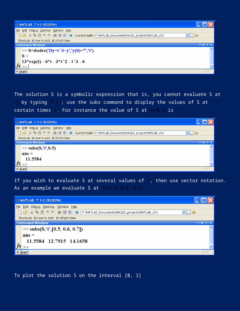
The solution S is a symbolic expression that is, you cannot evaluate S at t 0 by typing S(t 0); use the subs command to display the values of S at certain times t. For instance the value of S at t=0.5 is

If you wish to evaluate S at several values of t, then use vector notation. As an example we evaluate S at t=0.5 ,0.6 ,0.7 :

To plot the solution S on the interval [0, 1]

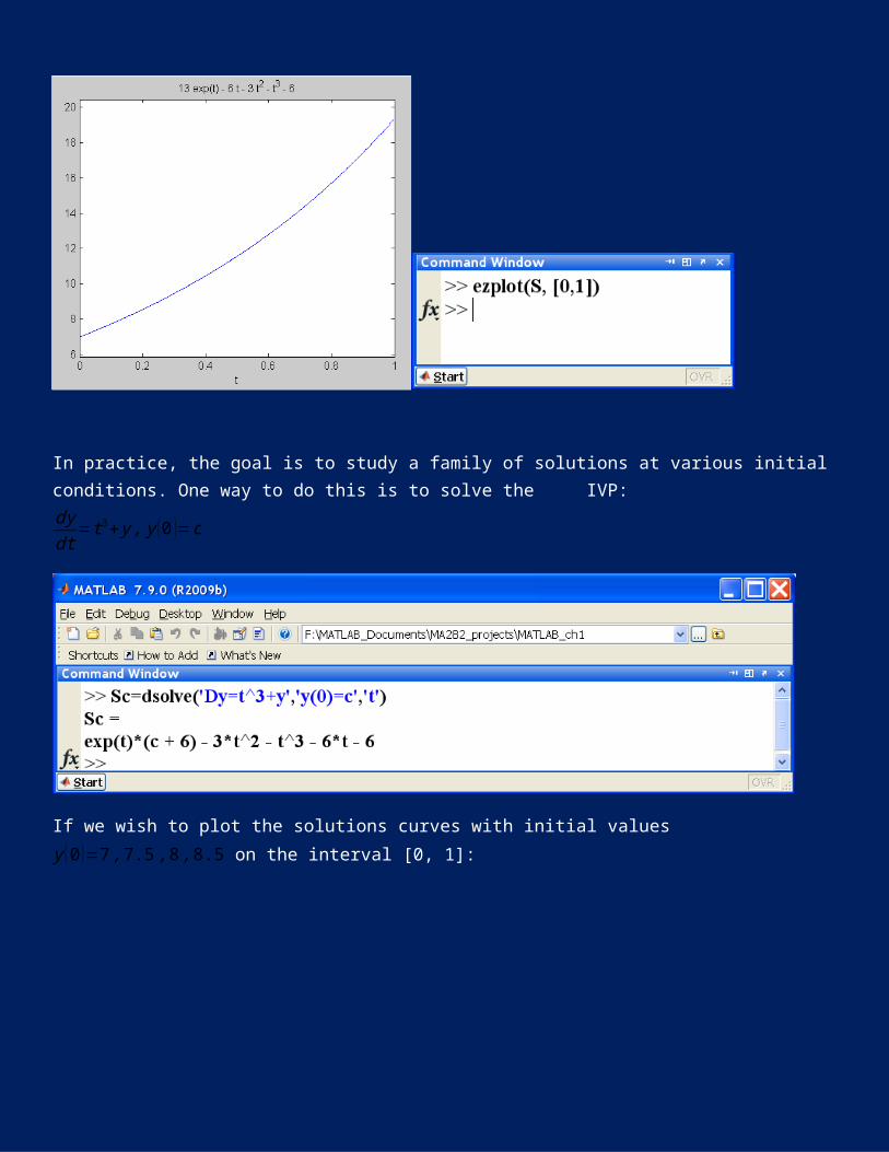
In practice, the goal is to study a family of solutions at various initial conditions. One way to do this is to solve the IVP: dydt =t3+ y , y (0 )=c

If we wish to plot the solutions curves with initial values y (0 )=7 ,7.5 ,8 ,8.5 on the interval [0, 1]:

Exercise MA282-1 (B. Hunt) (Solution at the end of document)Consider the initial value problem: t y '+3 y=5 t 2, y (2 )=5

a. Solve using the MATLAB function dsolveb. Plot the solution y (t ) on the intervals 0.5≤ t ≤5 and 0.2≤t ≤20. Determine the behavior of y (t ) as t approaches 0 from the right and as t becomes large.

c. Change the initial condition to y (2 )=3 and determine the behaviour of this solution, again by plotting on intervals such as 0.2≤t ≤20 and 0.5≤ t ≤5.

Exercise 282-2 (B. Hunt) (Solution at the end of document)a. Solve the initial value problem: y '−2 y=sin 2 t , y (0 )=cb. Use MATLAB to graph solutions for c=−0.5 ,−0.45 ,…,−0.05 ,0 on the interval [0, 1]. Use axis tight.c. Use MATLAB to graph solutions for c=−0.5 ,−0.45 ,…,−0.05 ,0 on the interval [0, 2.5]d. What happens to the solution curves as t increases?e. What effect small changes in initial data can have on the global behavior of solutions curves?

MA 282-Assignment #2: First Order Differential Equations -Part-2Qualitative Techniques1. Understanding the quiver commandThe quiver command allows us to draw vectors in the plane R2:

For instance, if we wish to draw the two vectors a¿<2,3>¿ and b=¿1,4>¿ and place them at the points (0 ,0) and (0 ,1) in R2, then we form the following four matrices:1. The x-positions matrix: [0,0]2. The y-positions matrix: [0,1]3. The x-components matrix: [2,1]4. The y-components matrix: [3,4]

If we type "quiver([0 0],[0 1],[2 1],[3 4])" in the command window, we see

Note that MATLAB automatically scales vectors so that they do not overlap. To prevent MATLAB from scaling vectors we add a zero to the script:

We can use the command axis to request that MATLAB draw the vectors and display them on a specific window. In this example we draw the vectors A and B and display them on the window 0≤ x≤10 ,0≤ y≤10:

To display a grid, simply type "grid on":

We can use the command "linewidth" to change the width of the vectors; in this example we multiply the original length by 1.5:

Important RemarkTo draw a single vector a=¿a1 , a2>¿ and place it at the point x=(x1 , x2), typequiver ([ x1 , x1 ] , [ x2 , x2 ] , [a1 , a1 ] , [a2 , a2 ]); that is we draw the vector a=¿a1 , a2>¿ twice.2. Slope FieldsConsider the equation dydt = y−t . If y (t ) is a solution of the equation, then f ( t , y )= y−t represents the slope of the tangent line to the graph of y (t ) at the point (t , y ). The following table gives the slopes of the tangent lines at three different points.

(t , y ) f (t , y )

(-1, 1)(-1, 0)(1, 4)

213

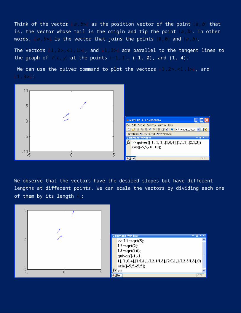
Think of the vector ¿a ,b>¿ as the position vector of the point (a ,b) that is, the vector whose tail is the origin and tip the point (a ,b). In other words, ¿a ,b>¿ is the vector that joins the points (0 ,0) and (a ,b).

The vectors ¿1 ,2> ,<1 ,1>¿, and ¿1 ,3>¿ are parallel to the tangent lines to the graph of f (t , y ) at the points (−1 ,1), (-1, 0), and (1, 4). We can use the quiver command to plot the vectors ¿1 ,2> ,<1 ,1>¿, and ¿1 ,3>¿:

We observe that the vectors have the desired slopes but have different lengths at different points. We can scale the vectors by dividing each one of them by its length Li:

The slope field of our differential equation can be obtained by repeating the same procedure for a large number of points. To do this we use the MATLAB commend meshgrid.In this example we plot the slope field of the above equation on the domain −4≤t ≤4, −3≤ y≤3.

We can obtain a better picture by reducing the length of the vectors by half:

Using the dsolve command, we see that the general solution of our equation consists of the family of functions y ( t )=t+1+ce t. The following figure shows the solutions for c=−2,−1 ,0 ,1 ,2 superimposed on the slope field.

ExamplePlot the slop field: y '=−t y2.A special attention should be directed to the second line and the way S was written. Make sure that use ".*" and ".^"

Exercise MA282-3 (B. Hunt) (Solution at the end of document)

Consider the critical threshold model for population growth y '=−(2− y ) y.a. Find the equilibrium solutions of the differential equation.b. Draw the slop field and use it to decide which equilibrium solutions are stable and which are unstable (y (t ) is stable if solutions that start near y (t ) converge to y (t )). Hint: modify [T,Y]=meshgrid(-4:0.2:4, -4:0.2:4)until you obtain a desirable slope

field.c. What is the limiting behavior of the solution if the initial population is between 0 and 2? Greater than 2?d. Use dsolve to find the solutions with initial values 1.5, 0.3, and 2.1. e. Plot the three solutions of part (d) together with the slop field on the same graph. Do the solutions follow the slope field as you expect it to?Exercise MA282-4 (Solution at the end of document)Consider y '=(α−1 ) y− y3.

a. Use solve to find the roots of (α−1 ) y− y3. Explain why y=0 is the only real root when α≤1, and why there are three distinct roots when α>1.b. For α=−2 ,−1,∧2, draw a direction field for the differential equation and deduce there is only one equilibrium solution. Is it stable?c. Do the same for α=1.d. For α=1.5 ,2 ,draw the direction field . Identify the equilibrium solutions and explain their stability.e. Explain: "As α increase through 1, the stable solution x=0 bifurcates into two stable solutions"

MA 282-Assignment #3: Numerical Solutions-the MATLAB Command ode45So far we have been using examples where the command dsolve was capable of producing explicit solutions of the differential equations.Now consider the IVP: y '= y− y2−0.2 sin ( t ) , y (0 )=2.If we type:

In this situation we use the numerical solver ode45 to find and plot approximate solutions for the equation.First we define an anonymous function (we could use an inline function):

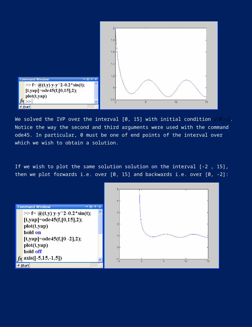
We will use the notation yap instead of y just to emphasis that the solution is an approximation one:

We solved the IVP over the interval [0, 15] with initial condition y (0 )=2. Notice the way the second and third arguments were used with the command ode45. In particular, 0 must be one of end points of the interval over which we wish to obtain a solution.If we wish to plot the same solution solution on the interval [-2 , 15], then we plot forwards i.e. over [0, 15] and backwards i.e. over [0, -2]:

Now suppose we want to plot a family of solutions with initial values y (0 )=0.1,0.3 ,0.5 ,1,2 over the interval [0, 15], then:

Similarly, we can plot the entire family on the interval [-2, 15] by solving forwards and backwards:

RemarkThe choice of axis is very important in producing a complete graph.ExampleConsider the initial value problem y '= y− y2−0.2 sin (t ) , y (7 )=0.5. Use ode45 to find an approximate solution over the interval [0, 15]. Plot the approximate solution together with an appropriate slope field.

Exercise MA282-5 (Solution at the end of document)Consider the differential equation y '= t

y .a. Use ode45 to calculate and plot an approximate solution to the initial value problem: y '= t

y, y (0 )=1 for 0≤ t ≤2b. Use dsolve to find an exact solution of the IVPc. Plot the exact and the approximate solution on the same graph. Can you distinguish between the two curves?d. Plot a family of solutions with initial values y (0 )=1.2 ,1.4 ,1.6 ,1.8 over the interval [-1, 2]

MA 282-Assignment #4: First-Order SystemsExample1 The predator-prey model

dRdt

=2R−1.2RF

dFdt =−F+0.9 RF

predicts cyclic population behavior for both the predator population described by F(t) and the prey population described by R(t). See Blanchard for more details.Equilibrium SolutionsThe solutions of the system {2 R−1.2 RF=0

−F+0.9 RF=0 are pairs of constant functions called equilibrium solutions to the system.We can use the solve command to find the equilibrium points of the above system by typing:

That is the equilibrium solutions are (R , F )=(0 ,0) and (R , F )=( 109

, 53 ).

R(t)- and F(t)-graphsIf we specify the initial conditions R0=1 and F0=0.5 we can use the MATLAB function ode45 to obtain approximate solutions to the system.Let P=(R ( t ) ,F (t ) ) ; we think of P as a vector whose components are R(t ) and F(t). For MATLAB, R(t ) is P(1) and F (t) is P(2). With this in mind, we begin by defining an anonymous function f whose components are the right hand side of the system:

Let us denote by Sap the approximate solution to the IVP; that is Sap=(R ( t ) , F ( t )) is an approximation to the actual solution of the system with the indicated initial conditions. If we wish to plot the first component of Sap i.e. R(t ) over the interval 0≤ t ≤15 then:

Similarly we can plot the component F (t) for 0≤ t ≤15:

We can plot the two solutions on the same graph as follows:

Phase PortraitThe plot of a solution (F ( t ) ,R ( t )) as a function of t would be a curve in the ( t ,F ,R )−space. The projection of this curve into the (F , R )−plane is called a trajectory or a solution curve. A trajectory is an example of a parameterized curve and is drawn by plotting (F ( t ) ,R ( t )) as t varies. A plot of a family of trajectories is called a phase portrait of the system.The solution curve for the predator-prey system dRdt

=2R−1.2RF

dFdt =−F+0.9 RF

corresponding to the initial condition (R0 , F0 )=(1,0.5) is

Making a phase portrait requires some planning. The best approach is to start by plotting the equilibrium solutions:

Next use a loop to add extra curves:

RemarkThe above phase portrait corresponds to the curves where (R (0 ) , F (0 ) )=(a ,b) for several values of a and b. Moreover we solved forwards from t=0 to t=6.If we change the initial conditions to (R (2 ) ,F (2 ) )=(a ,b) then it is necessary that we plot forwards and backwards otherwise we do not obtain complete curves.

Exercise MA282-6 (Solution at the end of document)Consider the predator-prey system {dRdt =2(1− R

3 )R−RF

¿

dFdt

=−2 F+4 RF . (See Blanchard section 2.1)

a. Use solve to find all the equilibrium solutionsb. Plot the solution curve corresponding to the initial conditions R (1 )=1 ,∧F (1 )=3.7 over the interval 0≤ t ≤30. For axis, use [0, 2, 0, 6].c. Describe the fate of the prey and predator populations based on the solution curve.d. Display graphs of the solutions R(t ) and F (t) corresponding to the initial conditions R (1 )=1 ,∧F (1 )=3.7 over the interval 0≤ t ≤30. Compare with part (c).

MA 282-Assignment #5: Vector Fields

Once again consider the predator-prey systemdRdt

=2R−1.2RF

dFdt =−F+0.9 RF

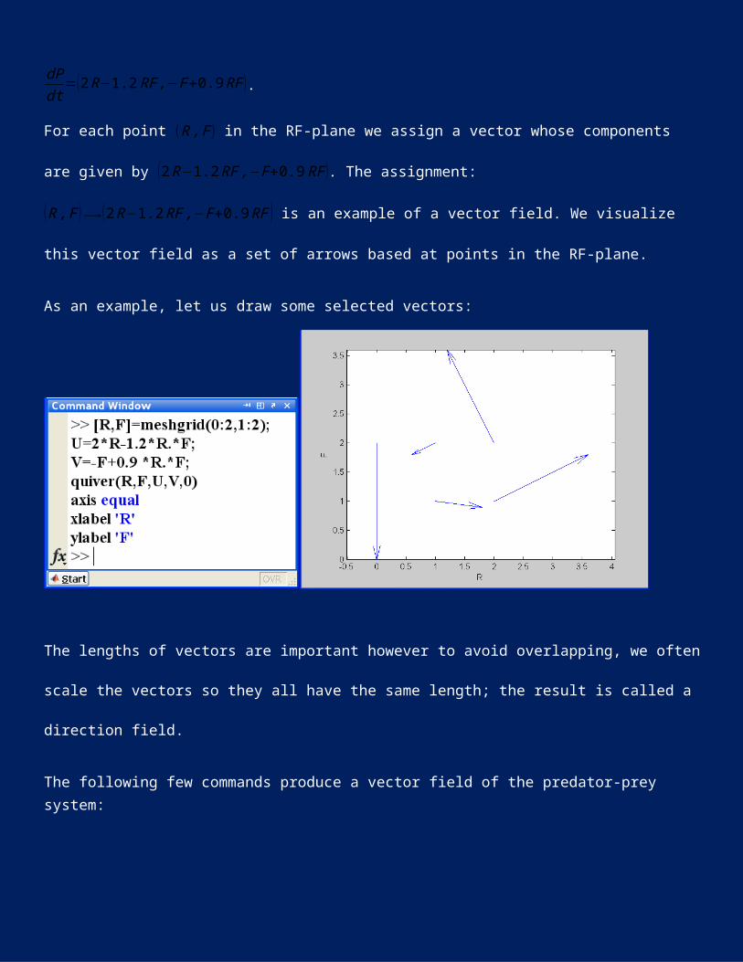
If we let P ( t )=(R (t ) , F( t)), then the system can be written in the formdPdt

=(2 R−1.2 RF ,−F+0.9 RF ).For each point (R , F) in the RF-plane we assign a vector whose components are given by (2 R−1.2 RF ,−F+0.9 RF ). The assignment: (R , F )⟶ (2R−1.2RF ,−F+0.9RF ) is an example of a vector field. We visualize this vector field as a set of arrows based at points in the RF-plane. As an example, let us draw some selected vectors:

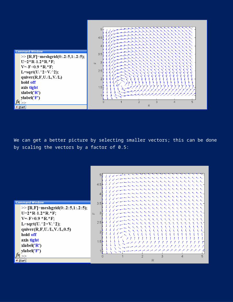
The lengths of vectors are important however to avoid overlapping, we often scale the vectors so they all have the same length; the result is called a direction field.The following few commands produce a vector field of the predator-prey system:

We can get a better picture by selecting smaller vectors; this can be done by scaling the vectors by a factor of 0.5:

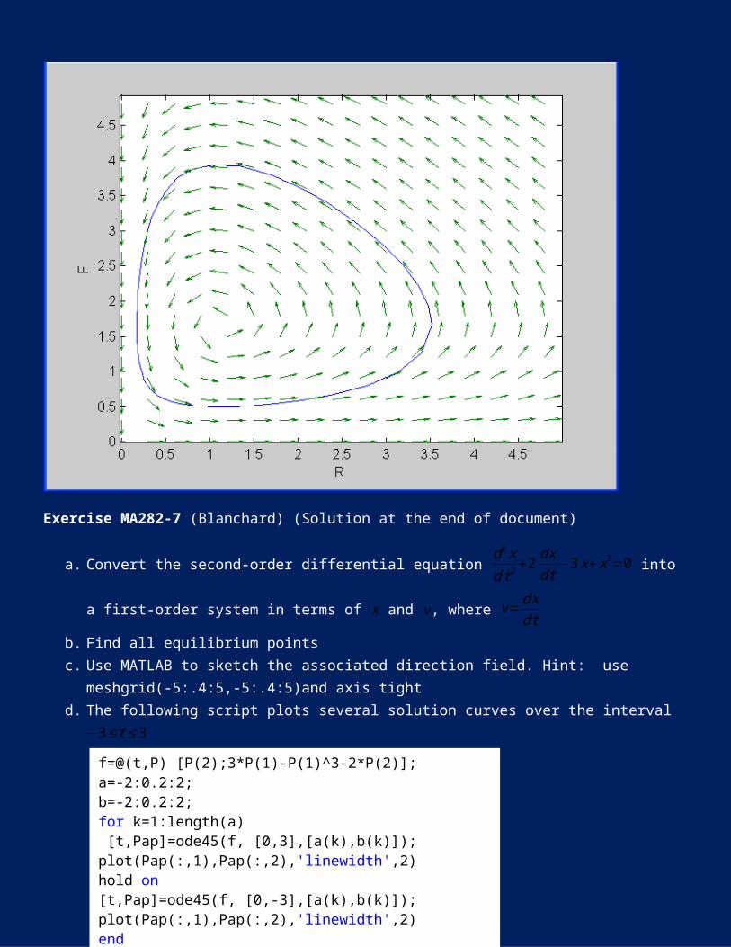
Now we plot the direction field together with the solution curve corresponding to the initial condition (R (0 ) , F (0 ) )=(1 ,0.5).

Exercise MA282-7 (Blanchard) (Solution at the end of document)a. Convert the second-order differential equation d2 x

d t 2 +2 dxdt

−3 x+x3=0 into a first-order system in terms of x and v, where v=dx

dt b. Find all equilibrium pointsc. Use MATLAB to sketch the associated direction field. Hint: use meshgrid(-5:.4:5,-5:.4:5)and axis tightd. The following script plots several solution curves over the interval −3≤ t ≤3

What are the initial conditions?e. Use the above script to plot a phase portrait together with the direction field of part c.f. Describe the behavior of the solutions?

f=@(t,P) [P(2);3*P(1)-P(1)^3-2*P(2)];a=-2:0.2:2;b=-2:0.2:2;for k=1:length(a) [t,Pap]=ode45(f, [0,3],[a(k),b(k)]);plot(Pap(:,1),Pap(:,2),'linewidth',2)hold on[t,Pap]=ode45(f, [0,-3],[a(k),b(k)]);plot(Pap(:,1),Pap(:,2),'linewidth',2)endhold offaxis([-5,5,-5,5])

MA 282-Assignment #6: Linear SystemsWe restrict our discussion to systems of the form

dxdt

=ax+by

dydt =cx+dy

where a ,b , c , d are constants.We let ¿(a b

c d) , Y (t )=( x (t)y (t)), and we write the system in the form dYdt =AY .

1. Strait -Line SolutionsRecall, if the matrix A has a real eigenvalue λ with associated eigenvector v, then the linear system dYdt =AY has the straight line solution Y (t )=eλt v.ExampleConsider the system dYdt =(2 2

1 3)Y .We use the MATLAB command eig to calculate the eigenvalues and their associated eigenvectors as follows.

The eigenpairs of the system are: λ1=1 , v1=[−21 ] and λ2=4 , v2=[11].

So the system has two straight- line solutions namely, Y 1 ( t )=et [−21 ]=[−2et

e t ] and Y 2 (t )=[e4 t

e4 t ].We can plot the direction field of the system exactly as we did for non-linear systems:

To plot half of the straight line solution, we type

Any multiple of the vector v1 is also an eigeinvector of λ1. In particular – v1 is an eigenvector and the lower half of the line is obtained by plotting the solution – et v1 .

Similarly we can plot the second straight solution as folows.

Please consult the textbook for detailed analysis of the importance of straight line solutions. Next we use MATLAB to solve linear systems in two different ways. We will focus on the technical parts; students should consult their textbooks to learn about the valuable information that eigenpairs pairs contain.

2. Solving Systems in Terms of EigenpairsCase I: two distinct real eigenvaluesExampleAs an example we solve the system dYdt =(−3 1

0 2)Y , Y (0 )=[25].We enter the coefficient matrix A=(−3 1

0 2) in MATLAB:

Next we use the command eig to calculate the eigenpairs of A:

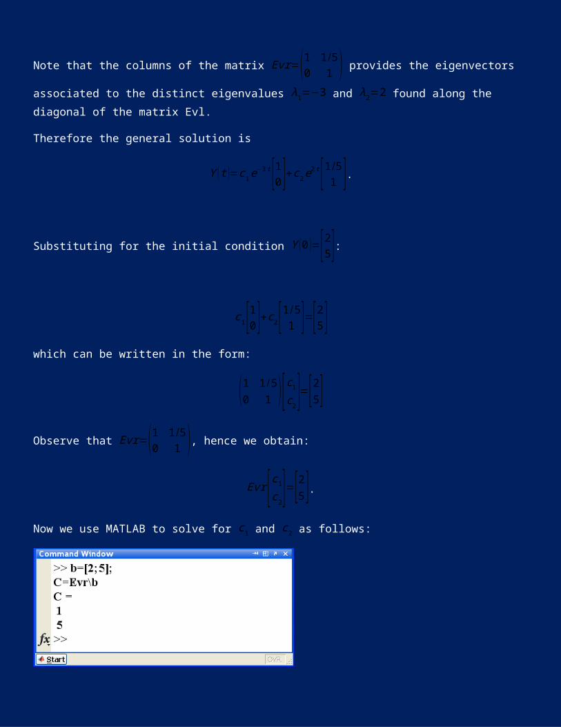
Note that the columns of the matrix Evr=(1 1/50 1 ) provides the eigenvectors associated to the distinct eigenvalues λ1=−3 and λ2=2 found along the diagonal of the matrix Evl.

Therefore the general solution isY (t )=c1 e

−3 t [10]+c2 e2 t [1 /5

1 ].

Substituting for the initial condition Y (0 )=[25]:

c1[10]+c2[1/51 ]=[25]

which can be written in the form:(1 1/50 1 )[c1

c2]=[25]Observe that Evr=(1 1/5

0 1 ), hence we obtain:Evr [c1

c2]=[25].Now we use MATLAB to solve for c1 and c2 as follows:

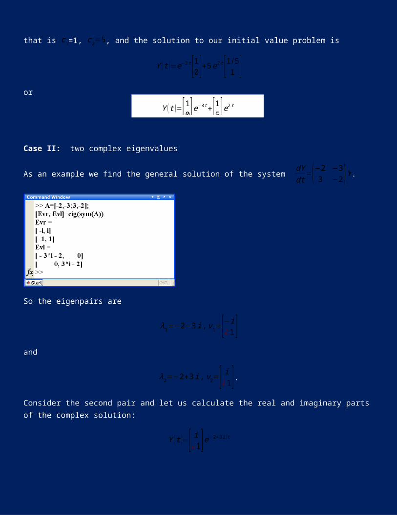
that is c1=1, c2=5, and the solution to our initial value problem is Y ( t )=e−3 t[10]+5e2 t [1 /5

1 ]or

Case II: two complex eigenvaluesAs an example we find the general solution of the system dYdt =(−2 −3

3 −2)Y .

Y ( t )=[10] e−3 t+[15]e2 t

So the eigenpairs areλ1=−2−3 i , v1=[−i

¿1]and

λ2=−2+3 i , v2=[ i¿1].

Consider the second pair and let us calculate the real and imaginary parts of the complex solution:Y (t )=[ i

¿1]e (−2+3 i) t

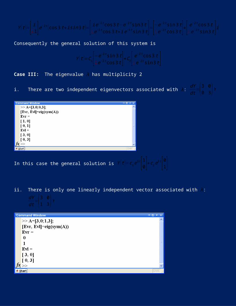
Y (t )=[ i¿1]e−2 t (cos3 t+isin3 t )=[ ie−2 t cos3 t−e−2 t sin 3 t

¿e−2t cos 3t+i e−2t sin 3 t ]=[−e−2 t sin 3 t¿e−2 t cos3 t ]+[ e−2 t cos3 t

¿e−2 t sin3 t ] iConsequently the general solution of this system is

Y ( t )=C1[−e−2 t sin 3 t¿e−2t cos 3t ]+C2[ e−2 t cos 3t

¿e−2 t sin 3 t ]Case III: The eigenvalue λ has multiplicity 2i. There are two independent eigenvectors associated with λ: dYdt =(3 0

0 3)Y

In this case the general solution is Y (t )=c1 e3 t [10 ]+c2 e

3 t [01 ]

ii. There is only one linearly independent vector associated with λ: dYdt =(3 01 3)Y

So there is one vector, v=[01 ], associated with λ=3. A particular solution is given by Y 1=eλt v=e3 t [01].A second solution is Y 2=te λt v+we λt, where ( A−λI )w=v.Note that Evr is just the vector v hence we can easily solve for w:

Therefore, Y 2=te λt v+we λt=te3 t [01]+[10]e3 t and the general solution is T (t )=C1Y 1 (t )+C2Y 2( t).3. Solving Systems using the command dsolveLet us consider the system discussed in Case III (ii): dYdt =(3 0

1 3)Y .That is the system

dxdt

=3 x

dydt =x+3 y

To find the general solution, we type

To solve the same system but with the initial conditions x (0 )=2 , y (0 )=5:

Exercise MA282-8 (Solution at the end of document)Let a be a real number different from 0 and consider the system

dxdt

=ax+4 y

dydt =ay

1. Use MATLAB to verify that the system has a double eigenvalue λ2. Use MATLAB to verify that there is only one eigenvector associated with λ3. Write a script that calculates the general solution of the system4. Verify your script by using dsolve to solve the system

MA 282-Assignment #7: Phase Portraits and Direction FieldsConsider the initial value problem

dxdt

=2x+2 y

dydt =x+3 y

, x (0 )=m , y (0 )=n .

We can use desolve to solve this IVP problem in terms of m and n:

As we have indicated before the outputs of the desolve command are symbolic expressions. We can use MATLAB to change those symbolic expressions into functions xf (t ,m,n) and yf ( t ,m,n). This can be done using the MATLAB command eval.Finally since we intend to plot solutions curves, we need to make sure that all expressions are vectorized ; has dots before * and /; otherwise t will be interpreted as a matrix and multiplications and divisions will not make any sense.

The following script should plot the straight-line solutions:

Let us plot the straight-line solutions together with some solutions curves:

Putting everything together by adding a direction field:

Exercise MA282-9 (Blanchard Ex 19, 3.3)Consider the initial value problem

dxdt

=−2x+ 12y

dydt =− y

, x (0 )=m, y (0 )=n.

1. Draw a direction field for the system. 2. Determine the type of the equilibrium point at the origin.3. Use dsolve to solve the IVP in terms of m and n4. Find all straight-line solutions5. Plot the straight-line solutions together with the solutions with initial conditions (m ,n )=(2 ,1 ) , (1 ,−2 ) , (−2 ,2 ) ,(−2,0)