vhdl design and simulation for embedded zerotree wavelet
TRANSCRIPT

Edith Cowan University Edith Cowan University
Research Online Research Online
Theses : Honours Theses
2000
VHDL design and simulation for embedded zerotree wavelet VHDL design and simulation for embedded zerotree wavelet
quantisation quantisation
Hung Huynh Edith Cowan University
Follow this and additional works at: https://ro.ecu.edu.au/theses_hons
Part of the Signal Processing Commons, Software Engineering Commons, and the Theory and
Algorithms Commons
Recommended Citation Recommended Citation Huynh, H. (2000). VHDL design and simulation for embedded zerotree wavelet quantisation. https://ro.ecu.edu.au/theses_hons/342
This Thesis is posted at Research Online. https://ro.ecu.edu.au/theses_hons/342

Edith Cowan University
Copyright Warning
You may print or download ONE copy of this document for the purpose
of your own research or study.
The University does not authorize you to copy, communicate or
otherwise make available electronically to any other person any
copyright material contained on this site.
You are reminded of the following:
Copyright owners are entitled to take legal action against persons who infringe their copyright.
A reproduction of material that is protected by copyright may be a
copyright infringement. Where the reproduction of such material is
done without attribution of authorship, with false attribution of
authorship or the authorship is treated in a derogatory manner,
this may be a breach of the author’s moral rights contained in Part
IX of the Copyright Act 1968 (Cth).
Courts have the power to impose a wide range of civil and criminal
sanctions for infringement of copyright, infringement of moral
rights and other offences under the Copyright Act 1968 (Cth).
Higher penalties may apply, and higher damages may be awarded,
for offences and infringements involving the conversion of material
into digital or electronic form.
Edith Cowan University Faculty of Communications, Health and Science
School of Engineering and Mathematics
Hung Huynh Bachelor of Computer Systems Engineering
First Class Honours
VHDL Design and Simulation for Embedded Zerotree Wavelet
Quantisation
© Huog Huyoh, 2000, ECU- Perth

USE OF THESIS
The Use of Thesis statement is not included in this version of the thesis.

I certify that this thesis does not incorporate without acknowledgment any material
previously submitted for a degree or diploma in any institution of higher education;
and that to the best of my knowledge and belief it does not contain any material
previously published or written by another person except where due reference is made
in the text.
Signature
Date 27 Jam/ 200{
,•
11

Acknowledgments.
I would like to take this opportunity to express my deepest gratitude to my supervisor,
Associate Professor Abdesselam Bouzerdoum for his fruitful support and guidance
throughout the course of this project. He spent a considerable amount of time out of
his busy schedule to ensure the success of my project.
I would also like to thank Dr. Hon Cheung who provided the supervision necessary
concerning the first half of the project. Also he provided invaluable literature related
to the project.
Last but not least, I would like to thank to my family and many friends, who have
inspired and showed much tolerating support throughout my course of study.
Hh,
Hung Huynh, Perth- 2000.
iii
Abstract
This thesis discusses a highly cfTcctivc still image compression algorithm - The
Embedded Zcrotrcc Wavelets coding technique, as it is called. This technique is
simple but achieves a remarkable result. The image is wavelet-transformed,
symbolically coded and successive quantised, therefore the compression and
transmission/storage saving can be achieved by utilising the structure of zerotrec. The
algorithm was lirst proposed by Jerome M. Shapiro in 1993, however to minimise the
memory usage and speeding up the EZW processor, a Depth First Search method is
used to transverse across the image rather than Breadth First Search method as
initially discussed in Shapiro's paper (Shapiro, 1993).
The project's primary objective is to simulate the EZW algorithm from a basic
building block of 8 by 8 matrix to a weB-known reference image such Leona of 256
by 256 matrix. Hence the algorithm performance can be measured, for instance its
peak signal to noise ratio can be calculated. The software environment used for the
simulation is a Very-High Speed Integrated Circuits - Hardware Description
Language such Peak VHDL, PC based version. This will lead to the second phase of
the project.
The secondary objective is to test the algorithm at a hardware level, such FPGA for a
rapid prototype implementation only if the project time permits.
iv

Table of Contents
Acknowledgment . . . . . . . . . . . . . . . . .. . . . . . . . . . . . . . . . . . . . . . . . . . . . . . . . . . . . . . . . . . . . . . . . . . . . 111
Abstract . . . . .. .. . . .. . . . . . . . . . . .. . .. .. . . . . . . . . . . . . . . . . . . . . . . . . . . . . . . . . . . . . . .. . . . . . . . . . . ... 1v
Table of Contents . . . . . . . . . . . . . . . . . . . . . . . . . . . . . . . . . . . . . . . . . . . . . . . . . . . . . . . . . . . . . . . . . . ... v
List of Figures ......................................................................... VIII
List of Tables . . . . . . . . . . . . . . . . . . . . . . . . . . . . . . . . . . . . . . . . . . . . . . . . . . . . . . . . . . . . . . . . . . . . . . . ... IX
Abbreviations . . . . . . . . . . . . . . . . . . . . . . . . . .. . . . . . . . . . . . . . . . . . . . . . . . . . . . . . . . . . . . . . . . . . . . . .. x
Notations . . . . . . . . . . . . . . . . . . . . . . . . . . . . . . . . . . . . . . . . . . . . . . . . . . . . . . . . . . . . . . . . . . . . . . . . . . . . . .. x1
Chapter I General Introduction . . . . . . . . . . . . . . . . . . . . . . . . . . . . . . . . . . . . . . . . . . . . ... I
1.1 Overview .............................................................. .
1.2 Project Objectives . . . . . . . . . .. . .. . . . . . . . . . . . . . . . . . . . . . . . . . . . . . . . . . . . . . . 2
1.3 Thesis Gutline . . . . . . . . . . . . . . . . . . . . . . . . . . . . . . . . . . . . . . . . . . . . . . . . . . . . . . ... 2
Chapter 2 An Introduction to Image Compression . . . . . . . . . . . . . . . . . . . . . . . . 4
2.1 Imagery in Perspective . . . . . . . . . . . . . . . . . . . . . . . . . . . . . . . . . . . . . . . . . . . . . .. 4
2.2 Perfonnance Measurement . . . . . . . . . . . . . . . . . . . . . . . . . . . . . . . . . . . . . . . . . . 5
2.3 Redundancy in Images .. . . . . . . . . . . . . . . . . . . . . . . . . . . . . ... . . . . . . . . . . . ... 6
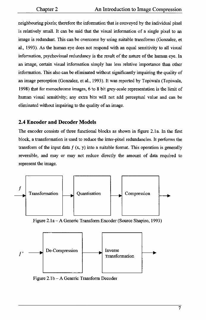
2.4 Encoder and Decoder Models . . . . . . . . . . . . . . . . . . . . . . . .. . . . . . . . . . . . ... 7
2.5 Lossless Compression Technique . . . . .. . . . . . . . . . . . . . . . . . . . . . . . . . . .. 8
2.5.1 Bit Plane Encoding . . . . . . . . . . . . . . . . . . . . . . . . .. . . . . . . . . . . . . .... 8
2.5.2 Run-Length Encoding . . . . . . . . . . . . . . . . . . . . . . . . . . . . . . . . . . . . ... 9
2.5.3 Huffinan Encoding . .. . . . . . . . . . .. . . . . . . . . . . . . . . . . . . . . . . . . . . . . 9
2.5.4 Arithmetic Encoding .. . . . . . . . . . . .. . . . . . . . . .. . . . . . . . . . . . . . . .. 9
2.5.5 Lossless Predictive Encoding ... . . . . . . . . . . . . . . . . . . . . . . . .... I 0
2.6 Lossy Compression Technique . . . . . . .. . . . . . . . . . . . . . . . . . . . .. . . . .. ... I 0
2.6.1 Vector Quantisation ......................................... 10
2.6.2 Discrete Cosine Transform . . . . .. . . . . .. . . . . . . . . . . . . . . . . . .... I 0
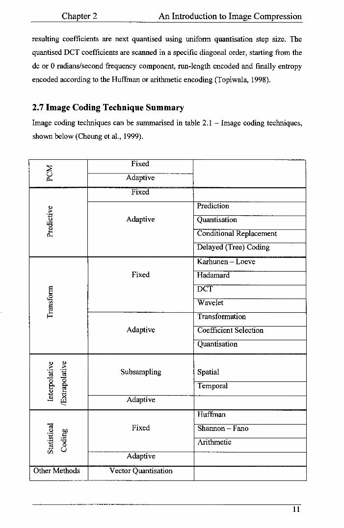
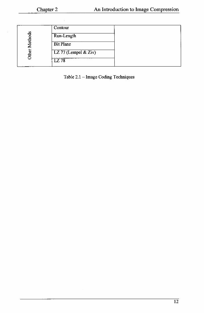
2.7 Image Coding Technique Summary ................................ II
Chapter 3 Wavelet Transform . . . . . . . . . .. . . . . . . . .. . . . . . . . . .. . . . . .. . . . .. . . . . . . .. 13
3.1 A Historical Milestone .. . .. . . . . .. . .. . . .. .. . . . . .. . . . . . . . . . . . ... . . . . ... 13
v
3.2 Fourier Transform.................................................... 14
3.3 Continuous Wavelet Transform . .. .. .. .. .. .. .. .. .. .. .. .. .. . .. .. .. .. 15
3.4 Discrete Wavelet Transform .. .. .. .. .. . .. . .. . .. .. .. . .. .. .. . .. . .. . .. . 18
3.5 Wavelet Transform in Image Processing.......................... 21
Chapter 4 EZW Algorithm . . . . . . .. . . .. . .. .. .. . . . . . . .. .. . .. . . . . . . .. . .. .. . . . . . . ... 23
4.1 Features of EZW Encoder........................................... 23
4.2 Decaying Spectrum Hypothesis.................................... 24
4.3 Subband Decomposition .......... .... ...... .. .. .... .. .... .. ......... 27
4.4
4.5
4.6
ChapterS
5.1
5.2
5.3
5.4
5.5
5.6
5.7
Chapter6
6.1
6.2
6.3
6.4
Chapter?
7.1
7.2
EZW Data Structure- Zerotree .. .. .. .. .. .. .. .. .. .. .. .. .. .. .. .. .. .. 28
Successive Approximation Quantisation . . . . . . .. . . . . . . . . . . . . . . . . .. 31
Adaptive Arithmetic Coding .... .. .... .. ...... ...... ...... .. .... .... 33
VHDL Implementation .. . .. . . .. .. .. .. .. . .. . .. .. .. .. . .. .. . .. . .. . .... 34
VHDL Overview .. . .. . .. .. .. .. . . .. .. .. .. .. .. .. .. .. .. .. . .. . .. . .. .. . .... 34
Design Consideration . . . . . . . . . . . . . . . . . . . . . . . . . . . . . . . . . . . . . . . . . . . . . . . . 3 7
Support Module .. .. .. .. .. .. .. . .. . .. .. .. .. . .. . .. .. .. .. .. .. .. .. . .. .. . . .. 40
Initialisation Module .. . .. .. .. .. .. . .. .. . .. . .. .. .. .. .. . .. .. . .. . . .. . .. .. 41
Encoder Module .. .. .. .. . .. .. .. . .. .. . .. .. .. .... .. .. . .. . .. . .. .. . . .. . .. . 42
Decoder Module . .. .. .. .. .. . .. . .. . . .. .. . .. . .. . .. .. .. .. .. .. .. .. .. . . . .. . 43
Th- .................................................................. M
Simulation Results .. .. .. .. .. .. .. .. .. .. .. .. .. .. .. .. .. .. .. .. .. .. .. ..... 46
Lenna- Who was she? .. .... .. .. .. .. .. .. .. .. .. .. .. .. .. .. .. .. .. .. .. ... 46
Test Image- Lenna ............ .......................... ............. 47
Test Modules .. . .. .. .. .. .. .. .. .. .. .. .. .. .. . .. .. .. .. .. .. .. . .. . .. . .. . .. .. 4 7
Embedded Transmission Test .. .. .. .. .. .. .. .. .. .. .. .. .. .. .. .. .. .. ... 48
Conclusion .. . .. .. . . . . . .. . . . . . . . . . . . . . . . . .. . . . . . . .. . . . . . . . . . . . . . . . . . . . . 54
Project Contribution .. .. .. .. .. .. .. .. .. .. . .. .... .. .... .. .. .. .. . .. .. .... 54
Further Direction...................................................... 55
Bibliography . . . . .. .. . . . . . . . . .. .. .. . .. .. . .. .. . .. . . . . . .. . . . .. . .. . . .. . . . . . . . . . . . . . . . . . . 57
VI
Appendix A
Appendix B
AppendixC
Listing A.O Module 0- Support VHDL Codes ............ 61
A. I Module I -Initialisation VHDL Codes ....... 62
A.2 Module 2- Encoder VIIDL Codes ............ 65
AJ Module 3- Test Encoder VIIDL Codes ...... 72
A.4 Module 4- Decoder VHDL Codes ............ 73
A.5 Module 5- Test Decoder VHDL Codes ...... 77
A.6 MatLab Converting Input Format Codes ..... 78
A.7 MatLab Converting Output Format Codes ... 79
Images B.! Original Image of Lenna . . . . . . . . . . . . . . . . . . . . . . . . 80
B.2 Embedded Image of Lenna . . . . . . . . . . . . . . . . . . .. . 8 I
C.! Typical Magnitude Output . . . . . . . . . . . . . . . . . . . . .. 86
C.2 Typical Symbolic Output . . . . . . . . . . . . . . . . . . . . .... 87
vi
List of Figures
2.1 A Generic Transform Coder and Decoder . . . . . . . . . . . . . . . . . . . . . . . . . . . . . . . . . ... 7
3.1 Uncertainty Principle in Wavelet Transform ...... .. . ... .. . . .. . ..... .. ...... 17
3.2 Subband Coding Algorithm . . . . . . . . . . . . . . . . . . . . . . . . . . . . . . . . . . . . . . . . . . . . . . . . . . .. 20
4.1 Parent-Child Dependencies of Subbands . . . . . . . . . . . . . . . . . . . . . . . . . . . . . . . . . . . . 25
4.2 Coefficients Scanned in Breadth First Search Method . . . . . . . . . . . . . . . . . .... 27
4.3 Coefficients Scanned in Depth First Search Method . . . . . . . . . . . . . . . . . . . . . .. 28
4.4 Flow Chart for Encoding a Coefficient for the Significance Map . . . . . . .. 30
5.1 VHDL General Design Process . . . . . . . . . . . . . . . . . . . . . . . . . . . . . . . . . . . . . . . . . . . . . ... 35
5.2 Abstraction Level in Structural Style . . . . . . . . . . . . . . . . . . . . . . . . . . . . . . . . . . . . . . . .. 36
5.3 Abstraction Level in B"havioural Style ........ .. . . ......... ... ... .. ......... 37
5.4 An Overview ofEZW DFS Architecture.................................... 38
5.5 DFS Scan Sequence . ......... .. ......... ... .... ...... .. ... ...... ... .......... ... 40
5.6 Encoder Pseudo Code . . . . . . . . . . . . . . . . . . . . . . . . . . . . . . . . . . . . . . . . . . . . . . . . . . . . . . . . . .. 42
5.7 Decoder Pseudo Code .. .... ...... .............. ........ ..... .... ... ..... ... . . .. 43
5.8 Shapiro Test Data . . . . . . . . . . . . . . . . . . . . . . . . . . . . .. . . . . . . . . . . . . . . . . . . . . . . . . . . . . . . . . . 44
5.9 SMAP Symbols . . . . . . . . . . . . . . . . .. . . . . . . . . . . . . . . . . . . . . . . . . . . . . . . . . . . . . . . . . . . . . . ... 44
5.10 SAQ Bit Stream . . . .. . . . . . . . . . . . . . . . . . . . . . . . . . . . . . . . . . . . . . . . . . . . . . . . . . . . . . . . . . . ... 45
5.11 Reconstructed Data . . . . . . . . . . . . . . . . . . . . . . . . . . . .. . . . . . . . . . . . . . . . . . . . . . . . . . . . . . . ... 45
6.1 OriginallmageofLenna ....................................................... 47
6.2 A Near Lossless Image of Lenna . . . . .. . . . . . . . . . . . . . . . . . . . . . . . . . . . . . . . . . . . . . . . 49
6.3 Lossy Image ofLenna for PSNR of 42.40 dB ... ... ............. .. ... .. . .. . 50
6.4 Lossy Image ofLenna for PSNR of35.03 dB.............................. 51
6.5 Lossy Image ofLenna for PSNR of26.61 dB.............................. 52
6.6 Lossy Image ofLenna for PSNR of 17.40 dB.............................. 53
VII

List of Tables
2.1 Image Coding Techniques .. . . . . . . . . . . . . . . . . .. . . . . . .. . . . . . . .. . . . . . . . . . . . . . . . . ... 11
4.1 Symbols for Zcrotrcc Structure . . . . .. . . . .. . .. . . . . .. . . . . . . .. . . . . . . . . . . . . . . . . . ... 29
5.1 Thresholds for 8-bit Coefticicnts ... ... . .. ... . .. .. . ... .... .... .. ..... . . . .. .. . 39
5.2 Alios ofSubband Levels lor an 8 by 8 Coefficient Matrix................ 39
5.3 Abstract Data Type lor Encoder and Decoder Units .. .. . . .. ... . ..... .. ..... 41
5.4 Signal Declaration lor Encoder Module...................................... 42
6.1 Embedded Transmission Test........................................... . . ... 49
IX

Abbreviations
ASIC
2D-DWT
ASCII
BFS
CWT
DCT
DFS
dpi
DWT
EOB EZW
FFT
FPGA
IBM
IEEE
IZ
JPEG
MSig
Neg
NTSC
PC
PCM
Pas
PSNR
QMF
RTL
SAQ
~DF
SMAP
SNR
STFT
VHDL
VLSI
WT
z ZTR
Application Specific Integrated Circuit
Two-Dimensional Discrete Wavelet Transform
American Standard Code for lnf{nmatiun Interchange
Breadth First Search
Continuous Wavelet Transform
Discrete Cosine Transform
Depth First Search
Dots Per Inch
Discrete Wavelet Transform
End-Of-Block Symbol
Embedded Zerotree Wavelets
Fast Fourier Transform
Field Programmable Gate Array
International Business Machine Corporation
Institute of Electronic and Electrical Engineers
Isotated Zero
Joint Photographic Experts Group
Marked Significant
Negative Significant
National Television Standards Committee
Personal Computer
Pulse Code Modulation
Positive Significant
Peak Signal to Noise Ratio
Quadrature Mirror Filter
Register-Transfer Language
Successive Approximation Quantisation
Significant Descendant Flag
Significant Map
Signal to Noise Ratio
Short Time Fourier Transform
Very-High Speed Integrated Circuits- Hardware Description Language
Very Large Scale Integration
Wavelet Transform
Zero
Zerotree Root
X

Notations
~ Coding Etlicicncy
'" Angular Frequency
~· Mother Wavelet Function
' Translation
Y (x.y) Coefficient y at coordinate of x and y
s {f(t)} Fourier Transfonn of Function f (t)
mse Mean Square Error
s Scale
a Input Variance
xi
Chapter 1 - General Introduction
1.1 Overview
The use of digital images first became generally visible to a broad community during
the early-unmanned lunar and planetary exploration missions, conducted by the
National Aeronautics and Space Administration in the mid-1960's. Since images have
been always used to enrich the textual information, especially when the computer
technology has been expanding at an ever-increasing rate. Digital images require a
large amount of memory space for storage and computing power for transmitting
and/or accessing image data. Hence there is an undeniable demand for better
methodology of image storage and very low rate transmission (i.e., smaller bandwidth
availability). Over the last forty years, many clever and efficient ways of sending both
still and moving images have been proposed and tested. Amongst them, the
Embedded Zero tree Wavelet Image Coding technique is an excellent method that can
be applied efficiently to a still image (Clarke, 1993).
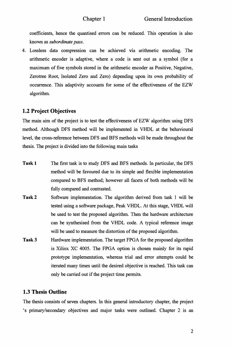
The EZW algorithm is a highly effective method; it is based on four principal
concepts.
1. Subband coding using discrete wavelet transform (DWT). The DWT technique is
used to overcome a long well known analysis tool of Fourier transform (i.e., time
information is lost). It offers a multi-resolution analysis where scale (i.e.,
frequency) and translation (i.e., time) can coexist in a transform domain.
2. Exploiting the similarity inherent in images using decay spectrum hypothesis. The
DWT coefficients are compared to a known threshold (to both encoder and
decoder), these coefficients are only coded if they are larger than the threshold,
otherwise these coefficients will be suppressed as an isolated zero or zerotree root
symbol. This operation is also known as dominant pass.
3. Successive-approximation quantisation. As significant coefficient symbols are
sent out, a binary stream of l's and O's will also be sent out to the arithmetic
encoder. These bits will be used to refine the reconstructed values of significant
1
Chapter 1 General Introduction
coefficients, hence the quantised errors can be reduced. This operation is also
known as subordinate pass.
4. Lossless data compression can be achieved via arithmetic encoding. The
arithmetic encoder is adaptive, where a code is sent out as a symbol (for a
maximum of five symbols stored in the arithmetic encoder as Positive, Negative,
Zerotree Root, Isolated Zero and Zero) depending upon its own probability of
occurrence. This adaptivity accounts for some of the effectiveness of the EZW
algorithm.
1.2 Project Objectives
The main aim of the project is to test the effectiveness of EZW algorithm using DFS
method. Although DFS method will be implemented in VHDL at the behavioural
level, the cross-reference between DFS and BFS methods will be made throughout the
thesis. The project is divided into the following main tasks
Taskl
Task2
Task3
The first task is to study DFS and BFS methods. In particular, the DFS
method will be favoured due to its simple and flexible implementation
compared to BFS method; however all facets of both methods will be
fully compared and contrasted.
Software implementation. The algorithm derived from task 1 will be
tested using a software package, Peak VHDL. At this stage, VHDL will
be used to test the proposed algorithm. Then the hardware architecture
can be synthesised from the VHDL code. A typical reference image
will be used to measure the distortion of the proposed algorithm.
Hardware implementation. The target FPGA for the proposed algorithm
is Xilinx XC 4005. The FPGA option is chosen mainly for its rapid
prototype implementation, whereas trial and error attempts could be
iterated many times until the desired objective is reached. This task can
only be carried out if the project time permits.
1.3 Thesis Outline
The thesis consists of seven chapters. In this general introductory chapter, the project
's primary/secondary objectives and major tasks were outlined. Chapter 2 is an
2
Chapter 1 General Introduction
introduction to digital image compression. This chapter identifies the redundancy
factors in image compression, several distortion metrics are also discussed. It then
investigates a typical model for encoding and decoding processes.
Chapter 3 examines the Fourier transform and its historical origin in mathematical
analysis. Both continuous and discrete wavelet transforms will be studied and how the
uncertainty principle, initially proposed by Heisenberg, can be extended to the theory
of wavelet transform. A comparison between the Fourier and wavelet transforms will
also be made.
In chapter 4, the EZW algorithm will be discussed in details. This chapter first focuses
on the main features of the EZW algorithm and the image analysis using this
algorithm. Second, it discusses the hypothesis of decaying spectrum. The rest of the
chapter is devoted to the EZW algorithm, particularly the data structure called
zerotree. It finishes with a brief discussion on the adaptive arithmetic coding.
Chapter 5 presents the EZW DFS implementation based on VHDL language. It
discusses all VHDL modules in details, including the EZW encoder and decoder
modules. Pseudo codes for modules are presented. The chapter concludes with the
testing aspect of the modules.
The simulation result will be the topic of chapter 6. The EZW algorithm derived and
implemented in previous chapters is tested using a reference test image of Lenna. A
brief background on the reference image is discussed. The next chapter examines a
near lossless reconstruction and several lossy reconstructions of the Lenna image
should the embedded transmission be terminated at certain point in the transmission.
A distortion measure is also presented for comparison purposes.
The final chapter, chapter 7 summaries the project contribution and highlights some
possible follow-up directions based on the knowledge gained in this project. It also
discusses a wish list to be accomplished if the time would otherwise be made
available.
3

Chapter 2 - An Introduction to Image
Compression
Pictorial information can be assimilated much more rapidly -and accurately than the
equivalent text or speech. Therefore, images generally are found in many aspects of
the modem society. Yet the data that comprises the image can easily grow at an
escalating rate. In many cases, it is impractical to store and transmit the images
without some form of compression. Image compression is a term that addresses the
issue of reducing the amount of data that is digitally required to represent the image.
In general, a signal can be compressed because it contains redundancies. A pure
random signal, for instance white noise, cannot be compressed because it contains no
redundancies. In this chapter, an overview of image compression will be discussed.
2.1 Imagery in Perspective
To appreciate the major gain in image compression, consider the following typical
examples (Cheung, et al., 1999)
An A4 size page of full text, scanned at 200 dpi will require 3.74 Mbits for
its storage. However, if this page is transmitted over Public Switched
Telephone Networks, it will take up to 6.54 minutes via a 9600-baud
modem.
In the case of still images, a frame of 35-mm film scanned at 2000 by 3000
pixel resolution and a requirement of 24 bits/pixel will require a
considerably large amount of storage, 18 Mbytes. An X-ray film of 14 by
17 inch size scanned at 5000 by 6000 pixel resolution with a requirement
of 12 bits/pixel will require 45 Mbytes.
In the case of motion images, a full-motion video of NTSC format will
require a bit rate of 150Mbits/second over the transmission medium to
achieve high-fidelity.
The examples above certainly highlight the need for still and motion image
compression means. It is required not only to achieve a saving in storage, but also to
reduce the needed bandwidth over the transmission medium. Data compression can be
4
Chapter 2 An Introduction to Image Compression
defined as the technique that is employed to remove irrelevant information and to
reduce the redundancy details in the raw data (V etterli, et al., 1995). The performance
of an image compression technique must be viewed with three aspects
Compression efficiency,
Image quality (ie. Distortion measurement), and
Computational cost.
Hence, many compression algorithms have been derived over the past years. The
differences between many algorithms are based on extracting/exploiting the data
redundancy/irrelevancy, compression efficiency, image quality and computational
cost. Yet, they can be categorised as lossless and lossy compression techniques.
2.2 Performance Measurement
Compression ratio can be used to measure the algorithm performance for both lossless
and lossy techniques. It is the ratio between the number of bits to represent the
original image and that of the compressed image. In lossless techniques, only a
modest amount of compression can be achieved. The reconstructed image coefficients
in lossless technique are numerically identical to the original image coefficients on a
pixel-by-pixel basis. All encoded and decoded coefficients are identical. Hence, this
technique yields a reversible compression process.
In lossy compression (also known as irreversible compression), the reconstructed
image will have some degradation relative to the original image. As a result, a much
higher compression ratio can be achieved as compared to lossless compression. For
lossy techniques, a number of distortion metrics can be used to measure the algorithm
performance. The mean squared error (mse) or distortion error can be defined as
1 N-� 2 mse = -( Z:1xi-Yil ) N i=O
Where Xi is the input value, Yi is the reconstructed value and N is the total number of
pixels in the image.
The signal to noise ratio is a measure of the separation between the signal and its error
( also known as noise)
SNR = 10 x log10 (Signal Power / Noise Power) in dB
5

Chapter 2 An Introduction to Image Compression
SNR = 10 x log10 ( cr2 / mse2) in dB
Where CJ is the input variance. And the peak signal to noise ratio is commonly used as
PSNR = 10 x log10 (M2 / mse) in dB
Where M is the maximum peak to peak value in the signal (typically 256 for an eight
bit image).
According to Shannon, the entropy of an information source S is defined as
H(S) = �Pi logr(pi) = -�Pi log p i
I I
Where Pi is the probability that a symbol Si will occur, and for the base r = 2, it has a
binary outcome. Therefore, the coding efficiency of an algorithm can be defined as
Tl= (Entropy / Average Code Length)
2.3 Redundancy in Images
The compression process is used to identify and remove the redundancy in data.
Various amounts of data may be used to represent the same amount of visual
information. When there are more data than actually required to represent a given
visual information, the data is known to contain data redundancy.
Data redundancy is a major concern in digital image compression field. Three basic
data redundancies can be identified and removed in digital image compression as
coding, inter-pixel and psycho visual redundancy.
The term coding redundancy refers to the fact that codes assigned to a set of events
are not based upon the occurrence probabilities of the events. It is certainly present
when image grey scale levels are represented with a natural binary code. In this case,
the same number of bits is assigned to both the most and the least probable values.
This can be overcome by using the adaptive coding technique. One such best-known
coding technique is Huffman coding (Gonzalez, et al., 1993).
Inter-pixel coding is a term that refers to the correlation between pixels in an image.
As the value of any given pixel can be reasonably predicted from the values of its
6
Chapter 2 An Introduction to Image Compression
Quantisation is the next block in the encoder model; it is used to assign the analog
values of the transformed input to predetermined binary values. It performs a
conversion between analog and digital representation. Yet the quantiser will reduce
the accuracy of the original data / (x, y). However, the psychovisual redundancy
elimination will be achieved within pre-established fidelity criterion. Finally, the last
block in the encoder model is the compression encoder, also known as symbol
encoder. Its function is to encode a fixed or variable length code to represent the
quantiser output. In many cases, a variable length code will be utilised to represent the
quantised data set. It will assign the shortest code words to the most frequently
occurring output value, and thus reduces coding redundancy. This operation is also a
reversible process. Upon completion of the symbol coding process, the input image
would have been processed to remove all redundancies; namely coding, inter-pixel
and psychovisual redundancies.
In figure 2. 1 b, the reverse process; decoder is shown. The decoder output is a
reconstructed image f ' (x, y). In general, f ' (x, y) may or may not be an exact replica
of the input image f (x, y). Some level of distortion is present in a reconstructed
image only if f' (x, y) is not an eigenfunction off (x, y). This is normally the case for
the lossy compression techniques.
2.5 Lossless Compression Techniques
2.5.1 Bit Plane Encoding
Bit plane encoding is a lossless compression technique. An image can be represented
by n x n matrix of pixels, where each pixel is quantised by m bits. By selecting each
bit from the same position in the binary representation of each pixel, a (m - 1) bit
plane image can be formed. For instance, the most significant bit of each pixel value
can be selected to generate an n x n binary image representing the most significant bit
plane. Repeating this process for the other bit positions, the original image can be
decomposed into a set of m in n x n bit planes. Each bit plane is therefore encoded
efficiently using a lossless binary compression technique such Run-Length Encoding
or Arithmetic Encoding.
8
Chapter 2 An Introduction to Image Compression
2.5.2 Run-Length Encoding
A Run-Length encoder replaces sequences of consecutive identical symbols with
three elements as
A single symbol.
A run-length count.
An indicator that signifies how the symbol and the count are to be
interpreted.
This coding algorithm applies equally well to sequence of bytes such as characters of
text, and to sequence of bits such as black and white pixels in an image. It is highly
effective when the data have many runs of consecutive symbols such computer data
files, which may contain repeated sequences of blanks or O 's. It is also effective
during the final stage of image and video data compression. Run-length encoding is
not adaptive, therefore its parameters must be carefully selected to match the data,
maximum compression only occurs when blanks are the most frequent character
found in repeated sequences.
2.5.3 Huffman Encoding
It is the best known and most widely used statistical entropy encoding technique
resulting from the study of information theory and probability. Its ideal is to observe
how frequently a particular symbol occurs. The compression can be obtained by
assigning shorter codewords to frequently occurring, more probable symbols, and
assigning longer codewords to infrequent occurring, less probable symbols. It was
used in the Morse code, and formalised by the work of Shannon, Fano and Huffman.
2.5.4 Arithmetic Encoding
To overcome the Huffman code limitation discussed above, the arithmetic encoding
technique was developed. It is a statistical entropy technique, and achieves near
optimal results for all symbol probabilities. This is achieved by merging the entire
sequence of symbols and encoding them as a single number. It also has another
advantage by making adaptive compression much simpler. It can be applied to a
variety of data, not just characters or particular types of image but to any information
that can be represented as binary digits.
9
Chapter 2 An Introduction to Image Compression
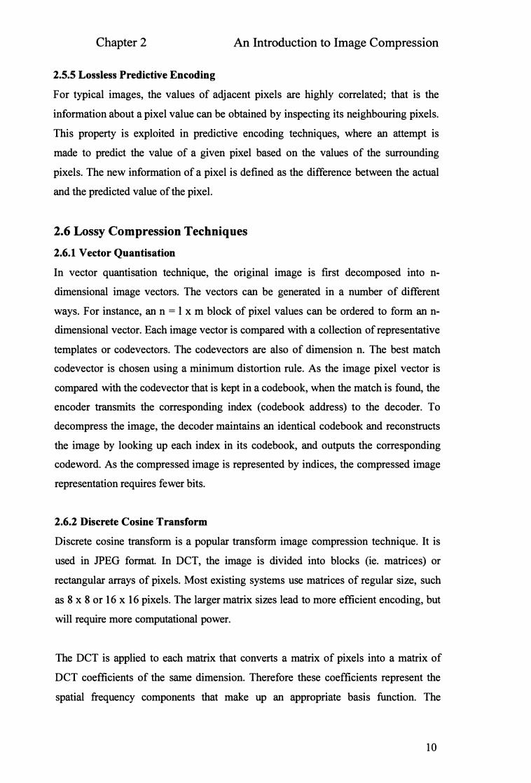
2.5.5 Lossless Predictive Encoding
For typical images, the values of adjacent pixels are highly correlated; that is the
information about a pixel value can be obtained by inspecting its neighbouring pixels.
This property is exploited in predictive encoding techniques, where an attempt is
made to predict the value of a given pixel based on the values of the surrounding
pixels. The new information of a pixel is defined as the difference between the actual
and the predicted value of the pixel.
2.6 Lossy Compression Techniques
2.6.1 Vector Quantisation
In vector quantisation technique, the original image is first decomposed into n
dimensional image vectors. The vectors can be generated in a number of different
ways. For instance, an n = 1 x m block of pixel values can be ordered to form an n
dimensional vector. Each image vector is compared with a collection of representative
templates or codevectors. The codevectors are also of dimension n. The best match
codevector is chosen using a minimum distortion rule. As the image pixel vector is
compared with the codevector that is kept in a codebook, when the match is found, the
encoder transmits the corresponding index (codebook address) to the decoder. To
decompress the image, the decoder maintains an identical codebook and reconstructs
the image by looking up each index in its codebook, and outputs the corresponding
codeword. As the compressed image is represented by indices, the compressed image
representation requires fewer bits.
2.6.2 Discrete Cosine Transform
Discrete cosine transform is a popular transform image compression technique. It is
used in JPEG format. In DCT, the image is divided into blocks (ie. matrices) or
rectangular arrays of pixels. Most existing systems use matrices of regular size, such
as 8 x 8 or 16 x 16 pixels. The larger matrix sizes lead to more efficient encoding, but
will require more computational power.
The DCT is applied to each matrix that converts a matrix of pixels into a matrix of
DCT coefficients of the same dimension. Therefore these coefficients represent the
spatial frequency components that make up an appropriate basis function. The
10
Chapter 3 - Wavelet Transform
Before investigating the wavelet transform, it is essential to have an understanding of
the Fourier transform, its advantages and drawbacks. Fourier transform has been used
as an analysis tool in the past many years; however, as a new technology emerged,
Fourier transform showed some shortcoming, since wavelet transform has been
derived to add a new dimension in the engineering analysis toolbox. In this chapter, a
brief mathematical aspect of Fourier transform will be discussed, its shortcoming and
it is then followed by an introduction of wavelet transform, both in continuous and
discrete forms. This new technique offers an important transform in digital image
compression, it is also known as multi-resolution analysis.
3.1 A Historical Milestone
Fourier analysis is a profoundly important tool in modelling many phenomena in
physics and engineering, as well as in modem medicine such as nuclear magnetic
resonance. It is a common term that is familiar in engineering profession. However,
let us go back in time to appreciate a historical milestone that is enable diversity of
modem time analysis. At the tum of the nineteenth century, the mathematical
description of heat conduction was a major outstanding problem. In 1807, a French
mathematician, Joseph Fourier (1768 - 1830) who lived during the Napoleonic era
and accompanied Napoleon on his Egyptian campaign, submitted a paper on this
subject to the prestigious Academy of Science of Paris. He was competing for a prize
that had been offered for the most successful analysis on this problem. Mathematical
geniuses as Laplace, Lagrange and Legendre evaluated the work and rejected it for a
lack of mathematical precision. And again in 1811, Fourier submitted a revised
version of his paper and was awarded the prize by the committee. However, the
academy still refused to publish the paper because many details were still unclear.
Even though Fourier is honoured by having his name attached to this important
engineering analysis tool, many of his contemporaries and immediate predecessors
contributed to his achievement, including Swiss mathematician Leonhard Euler (1707
- 1783); also known as the greatest analyst who ever lived (O'Neil, 1995).
13
Chapter 3 Wavelet Transform
3.2 Fourier Transform
Most of the signals in real life are time domain signals, that is, the signal is a function
of time. As the signal is plotted, the quantity of x is called the independent variable;
which normally is time, and the quantity of y is called the dependent variable of the
signal function; which normally is amplitude - This technique is called time
amplitude domain representation. A mathematical transform is applied to a signal to
obtain further information from that signal, which is not readily available in the
original signal. In other words, some properties of the signal in the new domain are
easier accessible than in the original domain. And in many real life cases, the most
distinguished information is hidden in the frequency content of the signal (Polikar,
1994 ). Furthermore, the desirable property of a transform is the ability to decorrelate -
that is, to eliminate the relation between transform coefficients in the transform
domain; thus the redundancy is reduced.
Fourier transform is used to translate the time-amplitude domain representation to
amplitude-frequency representation. Fourier transform can be defined as (O'Neil,
1995)
00
<; {/(t)}(co) = J f(t)e -jrot dt -00
In the amplitude-frequency domain, the plot is normally labelled for amplitude
variable as x and for frequency variable as y. It shows the frequency components that
are present in the original signal. However, this transform is only suitable for a
stationary signal, whose frequency components do not vary in time. In this case, one
does not require to realise at what times the frequency components are present, since
all the frequency components are present at all times. Furthermore, Fourier transform
can be used for non-stationary signal, whose frequency components vary in time. Yet,
the time information in Fourier transform based domain cannot be realised. In fact,
one cannot differentiate the amplitude-frequency domains between stationary and
non-stationary signals, which have the same frequency components. For transform
based signal compression, the main goal is to apply a transform that in most cases
provides a shorter description of a signal. In other words, a transform that decorrelates
14
Chapter 3 Wave let Transform
any signal in most cases is the best. The wavelet transform is such a transform. It can
be concluded that Fourier transform is not a suitable analysis tool for processing non
stationary signals, which are prevalent in digital image processing (Valens, 1999).
3.3 Continuous Wavelet Transform
The concept of wavelet transform was first proposed in 1984 by Goupillaud,
Grossman and Morlet. Wavelets are functions that can be generated from a single
function, the mother wavelet \jl, by dilation and translation. It can be defined as
1 * t - -r1/'(-r, s) = iTJ f x(t) 'I' (-)dt
vlsl s
The transformed signal is a function of two variables, 't and s, the translation and
scale; that is the time information and scale, respectively. The variables s and -r, scale
and translation, are the new dimensions after the wavelet transform. \jl(t) is the
transforming function, and it is called the mother wavelet. The term wavelet means a
small wave. The smallness refers to the condition that this function (it is the analysis
window) is of finite length. The term mother implies that the mother wavelet is a
prototype for generating the other analysis window functions. Scale used in the
equation refers to the resolution in the transform based domain, high scale means to
show the low frequency components and low scale means the high frequency
components that is a detailed information of a hidden pattern in the signal (normally
lasts a relatively short time).
Wavelet analysis is similar to Fourier analysis in the sense that it breaks a signal down
to its constituent components for analysis. Whereas the Fourier transform breaks the
signal into a series of sine waves of different frequencies, the wavelet transform
breaks the signal into its wavelets, scaled and shifted versions of the mother wavelet.
There are however some very distinct differences between the former and latter
transforms. In comparison to the sine wave, which is smooth, and of infinite length,
the wavelet is irregular in shape and compactly supported. It is these properties of
being irregular in shape and compactly supported which make wavelets an ideal tool
for analysing signals of a non-stationary nature. Their irregular shape lends them to
15

Chapter 3 Wavelet Transform
analysing signals with discontinuity or shape changes, while their compactly
supported nature enables temporal localisation of signal features. When analysing
signals of non-stationary nature, it is often beneficial to be able to acquire a
correlation between the time and frequency domains of a signal. The Fourier
transform, provides information about the frequency domain, however time localised
information is essentially lost in the process. The problem with this is the inability to
associate features in the frequency domain with their location in time, as an alteration
in the frequency spectrum will result in changes throughout the time domain. In
contrast to the Fourier, the wavelet transform allows the exceptional localisation in
both the time domain via translations of mother wavelet, and in the scale (that is
frequency) domain via dilations. The translation and dilation operations applied to the
mother wavelet are performed to calculate the wavelet coefficients, which represent
the correlation between the wavelet and a localised section of the signal. The wavelet
coefficients are calculated for each wavelet segment, yielding a time-scale function
relating the wavelets correlation to the signal.
The most important properties of wavelets are the admissibility and the regularity
conditions. It can be shown that square integrable function \j/(t) satisfying the
admissibility condition.
I 12 lf/({J)) J-- dm<+oo
1ml
The equation above can be used to first analyse and then reconstruct a signal without
loss of information. This implies that wavelets must have a band-pass like spectrum
(Sheng, 1996). The effect of this shifting and scaling process is to produce a time
scale representation. In comparison with the STFT, which employs a windowed FFT
of fixed time and frequency resolution, the wavelet transform offers superior temporal
resolution of high frequency components and scale (or frequency) resolution of the
low frequency components. This is often beneficial as it allows the low frequency
components, which normally show a signal its main characteristics or identity, to be
distinguished from one another in terms of their frequency content, while providing an
excellent temporal resolution for the high frequency components which add the
16
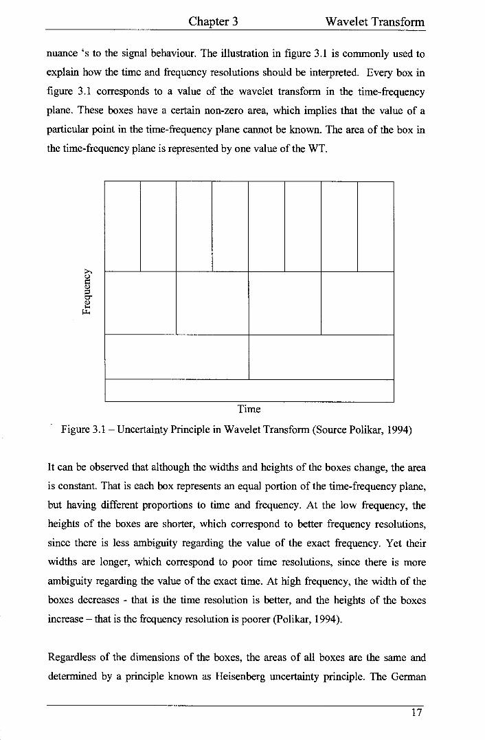

Chapter 3 Wavelet Transform ---------------~~~----~-~~
physicist Werner Heisenberg, who won the Nobel Prize in 1932, first proposed the
uncertainty principle. He stated that it is not possible to know simultaneously both the
exact momentum and position of a particle or to know its precise energy at a precise
time (Thornton ct al., 1993). This principle can be extended to WT theory. That is one
cannot reduce the areas of the boxes as much as he/she wishes due to Heisenberg 's
uncertainty principle. In other words, for a given mother wavelet the dimensions of
the boxes can be changed, but the area will remain the same - It is a compromise
belwec:n time and fr~quency resolutions.
3.4 Discrete Wavelet Transform
The continuous wavelet transform is the best transform that can be applied to a non
stationary signal; however, there are three properties that make it difficult to realise.
Firstly, the wavelet transform is calculated by continuously shifting scalable function
over a signal and calculating the correlation between the time and frequency. It will be
clear that the obtained wavelet coefficients will therefore be highly redundant. For
most practical applications, this redundancy should be removed. Secondly, without
the redundancy of the CWT, there is an infinite number of wavelets in the wavelet
transform (due to the integrating operator J ), the number of wavelets should be
reduced to manageable count. The third problem is that for most functions, the
wavelet transforms have no analytical solutions and they can be calculated only
numerically or by an analog computer. Thus, fast algorithms are required to be able to
exploit the power of the wavelet transform, and it is in fact the existence of these fast
algorithms that have many worldwide researchers studying the wavelet transform to
its full potential (Valens, 1999). These problems can be eliminated by using the
discrete wavelet transform. The DWT provides sufficient information for analysis of
the original signal; it is considerably easier to implement when compared to the CWT.
This can be accomplished by using the digital filtering technique. The continuous
wa¥elet transform is computed by changing the scale of the analysis window, shifting
the window in time, multiplying by the signal, and integrating over all times. In the
discrete case, filters of different cut-off frequencies are used to analyse the signal at
different scales. The signal is passed through a series of high and low-pass filters. The
resolution of the signal, which is a measure of the amount of the detail information in
the signal, is changed by the filtering operations, and the scale is changed by
18

Chapter 3 Wavelet Transform
upsampling and downsampling operations. Upsampling a signal corresponds to
increasing the sampling rate of a signal by adding new samples to the signal.
Similarly, downsampling a signal corresponds to reducing the sampling rate, or
removing some of the samples of the signal.
Filtering a signal is a mathematical operation of convolution of the signal with the
impulse response of the filter (Wade, 1994).
"' x[n]xh[n]= 2:x[k].h[n-k] k=-oo
The high-pass and low-pass filters are not independent of each other, and they arc
related by
g[L -1-n] = (-1)" .h[n]
Where g[n] is the high-pass filter, h[n] is the low-pass filter, and Lis the filter length.
Filters satisfying this condition are commonly used in signal processing, and they are
also known as the Quadrature Mirror Filters (QMF).
The DWT employs two sets of functions, called scaling function and wavelet
function, which are associated with low-pass and high-pass filters, respectively. The
decomposition of the signal into different frequency bands is simply obtained by
successive highMpass and low-pass filtering of the time domain signal. In effect, these
operations half the time resolution since only half the number of samples currently
characterises the entire signal. However, the decomposition doubles the frequency
resolution, since the frequency band of the signal spans only half the previous
frequency band, effectively reducing the uncertainty in the frequency by half. The
above procedure, which is also known as the subband coding, can be repeated for
further decomposition. At every level, the filtering and subsampling will result in half
the number of samples (and hence half the time resolution) and half the frequency
band spanned (and hence double the frequency resolution). Figure 3.2 illustrates this
procedure, where x[n] is the original signal to be decomposed, and h[n] and g[n] are
low-pass and high-pass filters, respectively. The bandwidth of the signal at every level
19
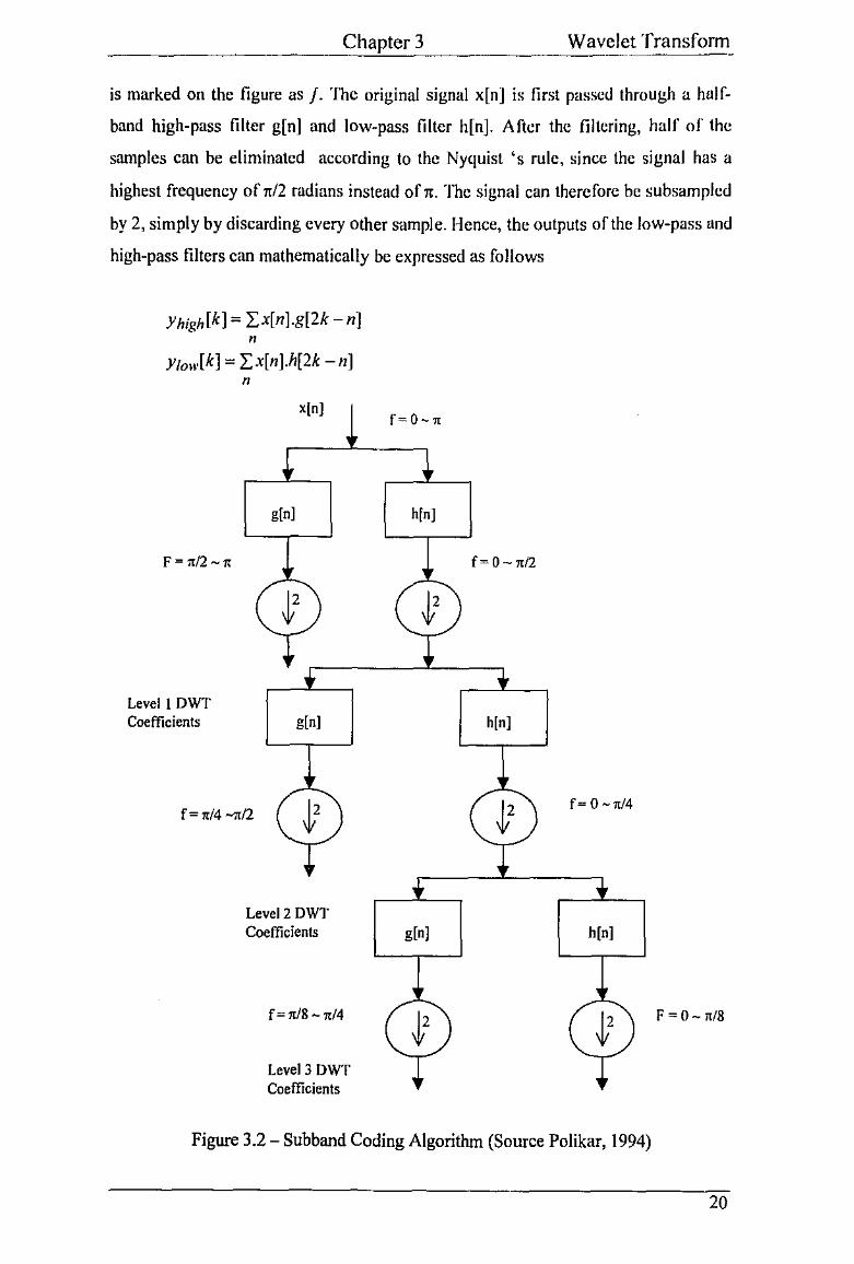
Chapter 3 Wavelet Transform ----------------~~~~--------~--
is marked on the figure as f. The original signal x[n] is first passed through a half
band high-pass filter g[n] and low-pass filter h[nJ. After the filtering, half of the
samples can be eliminated according to the Nyquist ~s rule, since the signal has a
highest frequency of rr/2 radians instead of rr. The signal can therefore be subsamplcd
by 2, simply by discarding every other sample. Hence, the outputs of the low-pass and
high-pass filters can mathematically be expressed as follows
Yhigh[k] = Ix[n].g[2k- n] n
Ylow[k] = Ix[n].h[2k -n]
F=1t/2-tt
Levell DWT Coefficients
n
x[n]
g[n]
~2
g[n]
f= 11'/4 -n/2 ~2
Leve12 DWT Coefficients
f = n/8 - n/4
Level3 DWT Coefficients
h[n]
f= 0 -nl2
h[n]
g[n] h[n]
~2
Figure 3.2- Subband Coding Algorithm (Source Polikar, 1994)
F=D-n/8
20
Chapter 3 Wavelet Transform
The ditTcrcncL~ of the DWT transfOrm from the Fourier transform is that the time
loculisation of these frequencies will not be lost. However, the time localbation will
have a resolution that depends upon which level they appear. If the main information
of the signal is located in the high frequencies, the time localisation of these
frequencies will be more precise, since they are characterised by more number of
samples. If the main information is located at very low frequencies, the time
localisation will not be very precise, since less samples are used to express signal at
these frequencies. This method in effect offers a good time resolution at high
frequencies, and good frequency resolution at low frequencies. The frequency bands
that are not very prominent in the original signal will have very low amplitudes, and
that part of the DWT signal can be discarded without any major loss of information,
thus allowing data reduction. The DWT provides a very effective data reduction
scheme, especially in image precessing (Vetterli et al., 1995).
3.5 Wavelet Transform in Image Processing
One of the classical problems in image processing is to select the size of the analysis
window in transfonning image pixels to corresponding coefficients. The criteria are to
select the best possible size for the anomalies and trends in the image. It is a
compromise selection. The animality is a signal behaviour that is more localised in the
time domain (or space domain in the case of image), and tends to spread in the
frequency domain. For instance, the perception of anomalies can be edges or object
boundaries. Conversely, the trend is a signal behaviour that is more localised in the
frequency domain, but tends to spread in the time domain. AsaP. example of this type,
image consistent background can be the typical case.
The anomalies nonnally have a small energy compared to an entire image, but to
human visual perception, these are significant as the ability to recognise the overall
image. The traditional transform can be used to decompose an image. However, to
achieve a reasonable fidelity at low bit rate transmission, a large number of non-zero
coefficients will be required which prohibit the realisation of the algorithm. That is a
large number of coefficients will require medium to high bit rate transmission. The
wavelet transform technique shows a promise transform that allows analysing the
21
Chapter 3 Wavelet Transform ~~-------=::.=:::.:_::___________ ·---
anomalies and trends on an equal basis, An extremely low bit rate is possible due to
more non-zero coefficients assigned to the anomalies (the anomalies normally have
the highest absolute value) and less resources assigned to the trends. In practice, the
linear correlation between the values of the coefficients in an image has been found to
be extremely small, implying that the wavelet transfonn is the currently best
transfonn used in image processing (Shapiro, 1993).
22
Chapter 4 - EZW Algorithm
The EZW algorithm was first proposed by Shapiro in 1993, since it has become a
prominent paper in image compression literatures using wavelet transform technique.
EZW stands for Embedded Zcrotrec Wavelet. In chapter 3, the wavelet transform was
examined in many details. The EZW encoder is based on progressive encoding to
compress an image into a bit stream with increasing accuracy. This means that when
more bits are added to the stream, the decoded image will contain more details.
Progressive encoding is also known as embedded coding. Zerotrec is a data structure
that can be used to compress an image against a predetermined threshold level - that
is the threshold is known to both the encoder and decoder. Coding an image using the
EZW algorithm results in a remarkably effective image compressor with the property
that the compressed data stream can have any bit rate depending upon the required
distortion. Any bit rate is only possible if there is infonnation loss in the encoding
process; hence the compressor is lossy. However, lossless compression is also
possible with the EZW encoder, only if a full bit stream is allowed to be transmitted.
In this chapter, many aspects of the EZW encoding/decoding processes will be
investigated in details.
4.1 Features ofEZW Encoder
The features of EZW encoder can be summarised as follows
A DWT is used to produce image coefficients by transforming pixel by pixel. The
DWT property of localisation (that is the pixel compactness) is utilised in the
transform process.
A data structure of zerotree is used to predict the insignificant coefficients at the
lower subbands. As the encoder is scanning across an image, the hierarchical tree,
which is used to represent the subbands will expand at the exponential rate. In
other words, the parent subband will have a further four children subbands. By
using zerotree structure, compression can be achieved in progressive transmission
where the bit stream can be terminated if the required distortion is met.
23
Chapt~r 4
Successive approximation is used to minimise the quantisution errors. This will be
implemented in the embedded coding, as lower bit rate is initially transmitted for
more significant coefficients.
Image details will be transmitted in the spirit of importance. That is coefficients
will be prioritied by the precision, magnitude, scale and spatial location in the
Image.
Adaptive arithmetic coding scheme is used to predict the absent coefficients as the
transmission is early terminated (that is the target bit rate or required distortion is
met). The adaptive arithmetic encoder statistically stores the symbol occurrences,
and makes a prediction based on this statistical data.
The algorithm can stop encoding as the target bit rate or required distortion is met.
It is an interesting point to note that the encoding process does not produce any
artefacts that would indicate where in the image the termination occurs.
The image compression using EZW algorithm is based on two key concepts
Natural images in general have a low-pass spectrum. When an image is
transformed, the wavelet coefficients will, on average, be smaller m higher
subbands than in lower subbands, as the higher subbands only add details.
Large wavelet coefficients are more important than small wavelet coefficients.
The two key concepts are exploited by encoding the wavelet coefficients in
decreasing threshold orUer, in several passes. For every pass, a threshold is selected
against which all the coefficients are measured. The outputs of each pass from the
EZW algorithm are the significance map SMAP, and successively approximated
values of significant coefficients SAQ.
4.2 Decaying Spectrum Hypothesis
The wavelet coefficient in one subband will have a pre-defined parent-child
relationship with the wavelet coefficients in other subbands. These relations will
define the appropriate symbols according to their spatial location and orientation. The
coefficient at the coarse scale is called the parent, and all coefficients corresponding
to the same spatial location at the next finer scale of similar orientation are called
children. For a given parent, the set of all coefficients at all finer scales of similar
24
Chapter 4 EZW Algorithm --
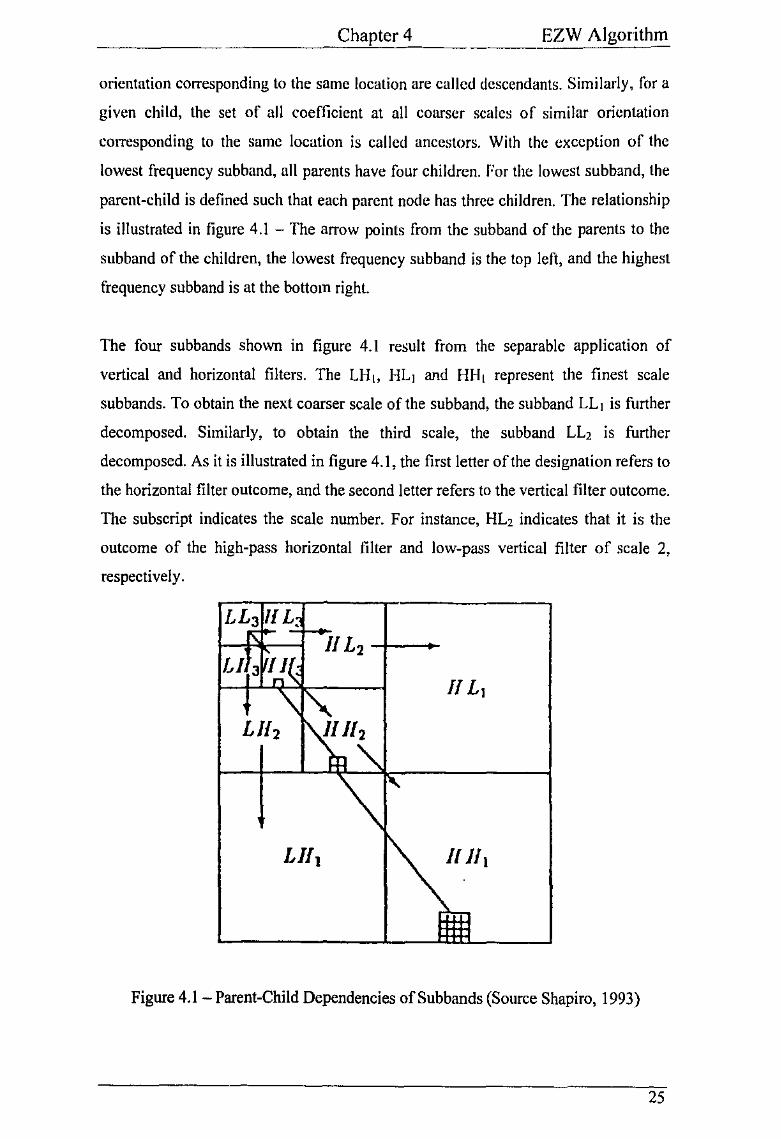
orientation corresponding to the same location are called descendants. Similarly, for a
given child, the set of all coefficient at all coarser scales of similar orientation
corresponding to the same location is called ancestors. With the exception of the
lowest frequency subband, all parents have four children. For the lowest subband, the
parent-child is defined such that each parent node has three children. The relationship
is illustrated in figure 4.1 -The arrow points from the sub band of the parents to the
subband of the children, the lowest frequency subband is the top left, and the highest
frequency subband is at the bottom right.
The four subbands shown in figure 4.1 result from the separable application of
vertical and horizontal filters. The LH 1, HL 1 and HH 1 represent the finest scale
subbands. To obtain the next coarser scale of the subband, the subband LL, is further
decomposed. Similarly, to obtain the third scale, the subband LL, is further
decomposed. As it is illustrated in figure 4.1, the first letter of the designation refers to
the horizontal filter outcome, and the second letter refers to the vertical filter outcome.
The subscript indicates the scale number. For instance, HL2 indicates that it is the
outcome of the high-pass horizontal filter and low-pass vertical filter of scale 2,
respectively.
/[ 111
Figure 4.1- Parent-Child Dependencies ofSubbands (Source Shapiro, 1993)
25

Chapter 4 EZW Algorithm
A tree structure, called spatial orientation tree, defines the spatial relationship on the
hierarchical decomposition. Figure 4.1 shows how the spatial relationship tree is
defined in hierarchical decomposition constructed with a recursive four-subband
splitting. Each node of the tree corresponds to a pixel and is defined by the pixel
coordinate.
The coetlicient is known to be significant if its absolute value is greater than the
current threshold index, otherwise it is insignificant. Moreover, the coefficient is a
positive significant if it is greater than zero, and a negative significant if it is less than
zero. A pre-determined sequence of thresholds may be used to save the threshold
transmission overhead; thresholds are stored at the decoder. It is called a bit plane
coding, as the pre-determined sequence is a sequence of powers of two; the thresholds
correspond to the bit value in the binary representation of the coefficients. The initial
threshold of bit plane coding can be defined as (Val ens, 1999)
Whereas max ( ) is the maximum coefficient value in the image, and y(x,y) denotes the coefficient at the coordinate of (x,y).
One of the aspects that have been used in image models is the hypothesis of decaying
spectrum. This hypothesis suggests that if a coefficient at a coarser scale is
insignificant, it is likely that all coefficients at finer scales will also be insignificant It
is analogous to the amplitude-frequency spectrum of a signal resulting from Fourier
transfonn. At higher frequency harmonics (that is much further away from the
fundamental component), their amplitudes will considerably be smaller than the
fundamental frequency amplitude. The hypothesis is a generalised statement - It
actually depends on the size of the analysis window. The hypothesis can be true at
some size of the analysis window, as the analysis window becomes larger (hence,
more coefficients have to be considered), the same truth may not be held. However,
the concept of a zerotree can be more general than the hypothesis of decaying
spectrum, as the structure of zero tree will be the topic of the next section. The zero tree
structure allows some deviation where the decaying spectrum will be violated.
26

Chapter 4 EZW Algorithm
4.3 Subband Decomposition
To process the coefficients, the scanning of coefficients is pcrfhrmcd in such a way
that no child is scanned before its parent. The EZW algorithm makes usc of the
ancestor-descendant relationships amongst the coefficients in difiCrcnt subbands in a
tree structure to efficiently encode the approximated values of the coefficients in a
sequence of passes through the coefficient tree. Shapiro initially proposed a search
method of exploring the width (it is the breadth of the tree structure) of the coefficient
tree first. hence the name of Breadth First Search. All coefficients in a given subband
are scanned before the scan moves to the next subband, as shown in figure 4.2 -
Coefficients scanned in Breadth First Search method. Each square in the figure
represents one pixel in the image.
,,, Hl, HLz
'"i HH,
ULt
LHz/ HH2
I
LH, I IIH1
Figure 4.2- Coefficients Scanned in Breadth First Search Method
(Source Shapiro, 1993)
In this method, a memory bank is used to store an intermediate data between the
dominant and subordinate passes. Each coefficient is scanned and its ancestors will be
stored in the allocated memory bani<. This memory baok will grow at ao exponential
rate, as the structure tree becomes larger. Furthermore, the EZW processor will
greatly slow down in accessing the allocated memory baok.
In contrast to the BFS, the Depth First Search method is more efficient in term of the
EZW processor speed. That is each coefficient cao be processed without having to
directly locate its ancestors, hence the memory bank is not required in this case.
Furthermore, the processor overall architecture is simple aod flexible. This lends itself
27
Chapter 4 EZW Algorithm
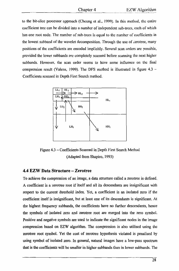
to the bit-slice processor approach (Cheung ct al., 1999). In this method, the entire
coeflicicnt tree can be divided into a number of independent sub-trees, each of which
has one root node. The number of sub-trees is equal to the number of cocfJicicnts in
the lowest subband of the wavelet decomposition. Through the usc of ;:crotrec, many
positions of the coefr1cients are encoded implicitly. Several scan orders arc possible,
provided the lower subbands arc completely scanned before scanning the next higher
subbands. However, the scan order seems to have some influence on the final
compression result (Valens, 1999). The DFS method is illustrated in figure 4.3 -
Coefficients scanned in Depth First Search method.
LL, HL, BL2 - 1---7
LH, HH HL,
Lllz IlHz
I~ , \
LH, I\ HH,
Figure 4.3 -Coefficients Scanned in Depth First Search Method
(Adapted from Shapiro, 1993)
4.4 EZW Data Structure- Zero tree
To achieve the compression of an image, a data structure called a zerotree is defined.
A coefficient is a zerotree root if itself and all its descendants are insignificant with
respect to the current llireshold index. Yet, a coefficient is an isolated zero if the
coefficient itself is insignificant, but at least one of its descendants is significant. At
the highest frequency subbands, the coefficients have no further descendants, hence
the symbols of isolated zero and zerotree root are merged into the zero symbol.
Positive and negative symbols are used to indicate the significant nodes in the image
compression based on EZW algorithm. The compression is also utilised using the
zerotree root symbol. Yet the cost of zerotree hypothesis violated is penalised by
using symbol of isolated zero. In general, natural images have a low-pass spectrum
that is the coefficients will be smaller in higher subbands than in lower sub bands. The
28
coefficients in higher subband will only add details. Furthermore, the analysis window
also plays a role in the validity of zcrotrce hypothesis. The analysis window size can
be enlarged to accommodate more image spectrum, however the complexity of
high/low subband decomposition will be increased, it will require a greater effort to
design, simulate and implement the system. It is a trade-off between the complexity
and spectrum covered. The proposed EZW DFS algorithm will be discussed in
chapter 5 - VHDL Implementation utilises an analysis window of an eight by eight
matrix, this will generate three-scale sub band decomposition.
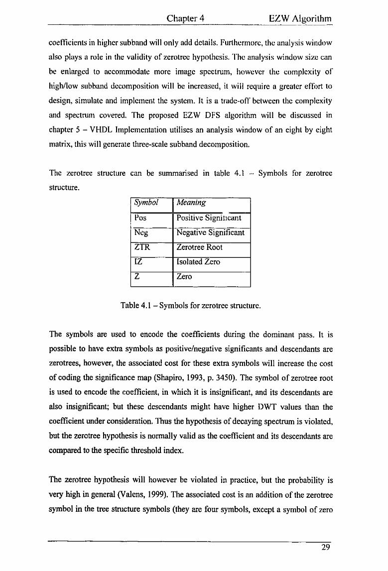
The zerotree structure can be summarised m table 4.1 - Symbols for zerotree
structure.
Symbol Meaning
Pos Positive Signit1cant
Neg Negative Significant
ZTR Zerotree Root
IZ Isolated Zero
z Zero
Table 4.1 -Symbols for zerotree structure.
The symbols are used to encode the coefficients during the dominant pass. It is
possible to have extra symbols as positive/negative significants and descendants are
zerotrees, however, the associated cost for these extra symbols will increase the cost
of coding the significance map (Shapiro, 1993, p. 3450). The symbol of zerotree root
is used to encode the coefficient, in which it is insignificant, and its descendants are
also insignificant; but these descendants might have higher DWT values than the
coefficient under consideration. Thus the hypothesis of decaying spectrum is violated,
but the zerotree hypothesis is normally valid as the coefficient and its descendants are
compared to the specific threshold index.
The zerotree hypothesis will however be violated in practice, but the probability is
very high in general (Valens, 1999). The associated cost is an addition of the zerotree
symbol in the tree structure symbols (they are four symbols, except a symbol of zero
29
+
_____________ C=ha::op:..:.tcr_~-------- _ _I:Z_\V_f\lgorithm_
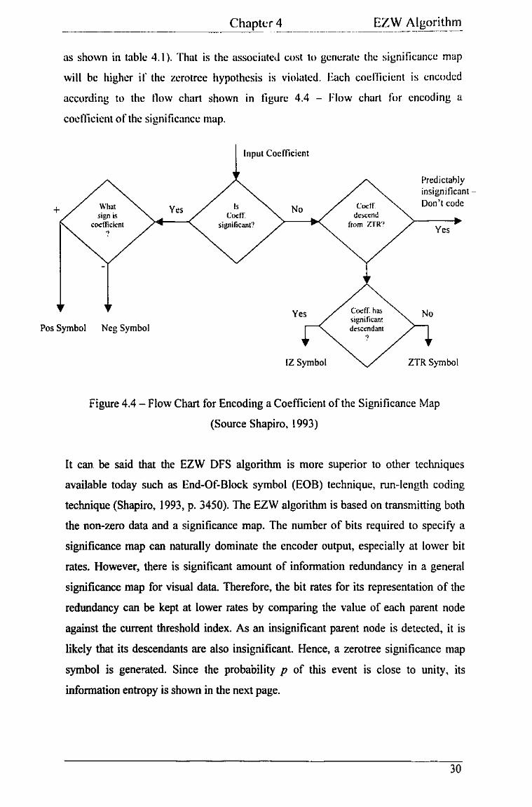
as shown in table 4.1 ). That is the associatcJ cost to generate the significance map
will be higher if the zcrotrcc hypothesis is violated. Each cocf"licicnt is encoded
according to the tlow chart shown in figure 4.4 - Flow chart for encoding a
coctlicient of the significance map.
What Yes sign is
coetlicicnt .,
Input Coefficient
,, Coo::ff_
No
signilicant'1
Yes
Predictahly insignificant-
Coclf Don't code
from ZTR'.' Yes
No
Pos Symbol Neg Symbol
Coeff has signili~ant descendant .,
IZ Symbol ZTR Symbol
Figure 4.4- Flow Chart for Encoding a Coefficient of the Significance Map
(Source Shapiro, 1993)
It can be said that the EZW DFS algorithm is more superior to other techniques
available today such as End-Of-Block symbol (EOB) technique, run-length coding
technique (Shapiro, 1993, p. 3450). The EZW algorithm is based on transmitting both
the non-zero data and a significance map. The number of bits required to specify a
significance map can naturally dominate the encoder output, especially at lower bit
rates. However, there is significant amount of information redundancy in a general
significance map for visual data. Therefore, the bit rates for its representation of the
redundancy can be kept at lower rates by comparing the value of each parent node
against the current threshold index. As an insignificant parent node is detected, it is
likely that its descendants are also insignificant. Hence, a zerotree significance map
symbol is generated. Since the probability p of this event is close to unity, its
infonnation entropy is shown in the next page.
30
___________ C_h_a_,.p_tc_r_4 ______ E_c_Z_W Algorithm
H(S)=-'i.;P;Iogp; -->0
That is, H(S) is very small. This implies that on average, a small amount of
information is transmitted, and this will translate to the average bit rate required for
the significance map is relatively low.
Yet, one or more of the children of the insignificance node is significant. In this case,
a symbol of an isolated zero is generated. The likelihood of this event is smaller, and
thus the bit rate for conveying this information entropy is higher. That is a drawback
of the EZW DFS algorithm, as the loss of information down the tree can generate
distortions should the lossy transmission be required.
4.5 Successive Approximation Quantisation
The role of quantisation is to represent the continuum of values with finite -
preferably small - amount of information. The quantiser is a function whose output
values are discrete and normally finite. Therefore, this implies that some loss of
information occurs at this stage. An ideal quantiser is one that represents the signal
with a minimum level of distortion.
The SAQ is performed during the scan of the subordinate pass. During this pass, the
output bits that are used to refine the true magnitudes of the coefficients found
significant during the dominant pass are specified to have an additional bit of
precision. The uncertainty interval is defined as the interval between two consecutive
thresholds, and the quantisation err0r of the coefficient is the difference between the
true magnitude and the quantised value after decoding the quantised bit stream
referenced up to and including the current threshold index. Thus during the
subordinate pass, the width of the effective quantised step size is halved as the bit
plane coding is used. Moreover, !I.e output bits of each magnitude can be encoded
using a binary decision with a I symbol indicating that the true value numerically falls
in the upper half of the last uncertainty interval, and a 0 symbol indicating the lower
half accordingly. The string of the symbols from this binary decision that is generated
during the subordinate pass is entropy-encoded.
31

___________ C=ha"'p'-'tec.:r_4 _____ ___:E:c:Z::,Wc.c Algorithm
In the decoding operation, each decoded symbol, both during a dominant and a
subordinate pass. refines and reduces the width of the uncertainty interval in which
the true value of the coefficient may occur. However, the initiJI reconstructed value of
a significant coefficient can be calculated as shown below should a 0 symbol of the
SAQ bit stream be received at the decoder
Reconstructed value~ 2_ x Current threshold index 4
Similarly, the initial reconstructed value ts shown below should a 1 symbol be
received at the decoder
Reconstructed value~ 7 x Current threshold index
4
As a sequence of threshold indices is used to test the coefficients of an image, the
quantised error will become smaller; that is the SAQ bit stream is used to refine the
actual magnitude value of coefficients found significant during the dominant pass. So
the current reconstructed magnitude value of a coefficient can be calculated as
I Current reconstructed value =Last reconstructed value± (- x Current
4
threshold index)
Whereas a positive sign (+) is used should a I symbol of the SAQ bit stream be
received at the decoder. Similarly, a negative sign(-) is used should a 0 symbol be
received at the decoder.
The encoding can stop when some target stopping condition is reacher!, such as when
the bit budget is exhausted or when the required distortion is met. The encoding can
cease at any time and the resulting bit stream contains all lower rate encodings.
Should the SAQ bit stream be truncated at an arbitrary point, there may be bits at the
end of the code that do not decode to a valid symbol as the codeword has been
32
Chapter 4 EZW Algorithm ---
truncated. In this case, these bits do not reduce the width of the uncertainty interval;
that is these bits are not used in the decoding process. Therefore, terminating the
decoding of an embedded bit stream at a specific point in the bit stream produces the
same image thal would have resulted had that specific point been the initial target rate.
This can be achieved without producing any blocking artefact in the reconstructed
image.
4.6 Adaptive Arithmetic Coding
The two outputs from EZW encoder are SMAP and SAQ streams. SMAP stream is
generated during the dominant pass, and SAQ stream is generated during the
subordinate pass. In the subordinate pass, the symbols of 1 's and O's are used to
indicate the significant coefficient values falling within the upper or lower half of the
width, respectively. Furthermore, the symbols used in the dominant pass depend upon
the condition of the coefficient values and the current threshold indices. As a zerotree
root is detected, there are only three symbols used; Pos, Neg and IZ, otherwise four
symbols are used; they are Pos, Neg, IZ and ZTR. Thus a maximum of four symbols
is used depending on the current scan is a dominant or subordinate pass. The final
encoder is normally an adaptive arithmetic encoder as theoretically it is the best
possible encoder; based on information theory. The adaptive encoding technique is a
compromise between speed, compression ratio and image quality. Therefore, the
SMAP and SAQ streams are best encoded by an adaptive arithmetic encoder, as all of
the possibilities typically occur with a reasonably measurable frequency for the
symbols. This adaptivity accounts for the effectiveness of the EZW algorithm. In
other words, the encoder will learn the source statistics as it progresses. So it can be
said that the source model is incorporated into the actual bit stream.
At the decoder end, the same source statist:. s are kept to monitor the incoming bit
stream. When the transmission stops as the stopping condition is reached (that is the
distortion rate or the target bit rate is met), the source statistics can be used to predict
the values of the coefficients that are not transmitted. This certainly yields a higher
distortion rate.
33

Chapter 5 - VHDL Implementation
As the size and complexity of digital systems increase, design methodology has to be
improved. A higher level of abstraction to capture designs is not a luxury, but it is a
necessity. VHDL stands for VHSIC Hardware Description Language and is becoming
increa..;;ingly popular as a way to express complex digital concepts for both simulation
and synthesis. It can be used to describe digital logic for implementation in FPGA's or
ASIC's. It is a high level programming language that allows complex design concepts
to be expressed as computer programs; VHDL allows the behaviour of complex
electronic circuits to be captured into a design system for automatic circuit synthesis
or for system simulation. This chapter focuses on the VHDL implementation of the
EZW DFS algorithm. The chapter first presents an overview of the VHDL language.
Second, it describes how the encoder is mapped into a structure data type in VHDL.
The rest of the chapter is on how the decoder is implemented in VHDL. The listings
of the VHDL code on this chapter can be found in appendix A.
5.1 VHDL Overview
VHDL language is used to describe the hardware for the pu~JOse of simulation,
modelling, testing, design and documentation of digital systems regardless of their
complexity. It was initially created for the United States Department of Defence in the
summer of 1983 (by IBM, Texas Instruments and Intermetrics Corporations), and fom
years later in December of 1987, IEEE formally approved it as a standaro ... . ... ,e
description language. Today, it is an international standard, reviewed by IEEE every
five years (Navabi, I 993, pl6).
The design of the system is functionally described with VHDL. It is expressed in a
high level programming language structures such structural and/or behavioural styles.
These styles differ primarily in how closely they relate to the underlaying hardware.
In the structural style, the design concept is described at the hardware level, which
logic gates are interconnected. This provides designers an environment to utilise the
hardware resources. It also provides an excellent tool to debug the system timing
issue. Conversely in the behavioural style, the concept is abstractly described at the
34

Chapter 5 VHDL Implementation
mathematical/logical expression. That is designers arc only concerned with the system
conceptual specification. These two styles will complement one another in the design
process. Next, the simulation is used to verify the functionality of the design. This
allows designers to make faster functionally correct designs, to explore more
architecture trade-offs, anrl to have more impacts on the designs. The VHDL dcsign
process is shown in figure 5 .I - VHDL general design process.
Description
Simulation
Synthesis
Figure 5.1 - VHDL General Design Process
After the functions match the requirements, the VHDL code is synthesised to generate
schematics or equivalent netlists. The netlist can be used to layout the circuit and to
verify the timing requirement. The design changes can be made by modifying VHDL
code or changing the constraints such as timing, chip area in the synthesis. Moreover,
VHDL supports structural and behavioural styles, as illustrated in figures 5.2 and 5.3,
respectively. Each figure shows the levels of abstraction for its style. At the most
abstract level, the function of the system can be described in terms of an algorithm, as
shown in figure 5.3. This level of functional modelling is also called behavioural
modelling. At this top level of structural abstraction, the structure of the system can be
described as an interconnection of such components as processors, memories and
input/output devices. This level is also known as the Processor Memory Switch level.
35

Chapter 5 VHDL Implementation
The next level of abstraction in structural domain is rcJCrrcd to register transfer level,
composed of a data path and a control section. The data path contains data storage
registers, and the control section sequences operation of the data path components. In
the ftmctional domain, a register-transfer language (RTL) is used to specify the
operation of the system at this level. Storage of data is represented using register
variables.
Processor-Memory Switch
Register-Transfer
Gate
Transistor
Level Of
Abstraction
Figure 5.2- Abstraction Level in Structural Style (Source Ashenden, 1996, p 4)
The third level of abstraction is the conventional logic level. At this level, the
structure is modeled using interconnections of gates, and function is modeled by
Boolean equations, or truth tables. At the most detailed level of abstraction, structured
model is described using individual transistors, function using the differential
equations that relate voltage and current in circuit. There are many levels involved in
the design process, however a number of software vendors that support the automatic
transfonnation between different levels are available. This new design approach and
methodology has improved the design process by shortening design time, reducing the
36

Chapter 5 VHDL Implementation
number of design iterations, and increasing the design complexity that designers can
manage.
Algorithm
Register-Transfer Language
Boolean Equation
Differential Equation
Level Of
Abstraction
Figure 5.3- Abstraction Level in Behavioural Style (Source Ashenden, 1996, p4)
5.2 Design Consideration
In this project, the EZW DFS algorithm is implemented in Peak VHDL Professional
Edition, version 5.1la. The EZW DFS architecture is divided into a number of
manageable modules called hierarchical levels. These hierarchical levels are
numbered orderly starting from 0. Thus a higher hierarchical level can utilise a
function/procedure declared in a lower hierarchical level. The hierarchical levels 2
and 4 are EZW encoder and decoder units, respectively. The encoder and decoder
units are initialised at power-up by module level 1, and structurally supported by
module level 0. These modules will be examined in this chapter, except module levels
37
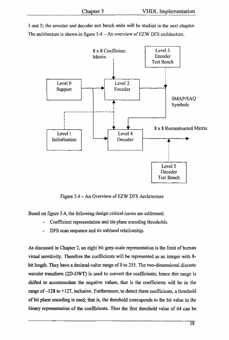
Chapter 5 VHDL Implementation
3 and 5; the encoder and decoder test bench units will be studied in the next chapter.
The architecture is shown in figure 5.4 -·An overview of EZW DFS architecture.
8 x 8 Cocflicicnt Lcvel3 Matrix Encoder
Test Bench
Leve!O Level2 Support Encoder
SMAP/S ~ Symbols '
AQ
:·-·--------------___________ ,
' ' ' ' i ;
' y 8 x 8 Reconstruct ed Matrix Levell Leve14
Initialisation Decoder
LevelS Decoder
Test Bench
Figure 5.4- An Overview ofEZW DFS Architecture
Based on figure 5.4, the following design critical-issues are addressed.
Coefficient representation and bit-plane encoding thresholds.
DFS scan sequence and its sub band relationship.
As discussed in Chapter 2, an eight bit grey-scale representation is the limit of human
visual sensitivity. Therefore the coefficients will be represented as an integer with 8-
bit length. They have a decimal-value range of 0 to 255. The two-dimensional discrete
wavelet transform (2D-DWT) is used to convert the coefficients; hence this range is
shifted to accommodate the negative values, that is the coefficients will be in the
range of -128 to+ 127, inclusive. Furthermore, to detect these coefficients, a threshold
of bit plane encoding is used; that is, the threshold corresponds to the bit value in the
binary representation of the coefficients. Thus the first threshold value of 64 can be
38

Chapter 5 VHDL Implementation
used to detect the highest coefficients ( ~ 128 or + 127) as positive/negative significants;
the second threshold value of 32 can be used next in the dominant pass. However, the
initial threshold of bit plane encoding is defined in Chapter 2. The sequence of
thresholds used in the EZW DFS algorithm is shown in table 5.1 -Thresholds for 8-
bit coefficients.
Threshold
Order Value
7 64
6 32
5 16
4 8
3 4
2 2
I I
0 0
Table 5.1 -Thresholds for 8-bit coefficients
In order to encode an image, a pre-determined scan sequence of EZW DFS is used to
transverse across the image. The analysis window of an 8 by 8 coefficient matrix is
chosen due to the complexity of DFS decomposition. For an 8 by 8 matrix, there are
four sub band levels to be considered. They are defined as shown in table 5.2 - Alias
of subband levels for 8 by 8 coefficient matrix.
Decomposed Subbands
Level Alias Meaning
I" node Main Parent ancestor
znd node Second Parent 1st descendant
3rd node First Child znd descendant
4ili node Last Child 3 '' descendant
Table 5.2- Alias of Sub band Levels for an 8 by 8 Coefficient Matrix
39
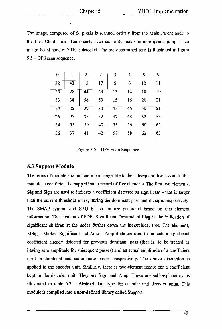
Chapter 5 VHDL Implementation
The image, composed of 64 pixels is scanned orderly from the Main Parent node to
the Last Child node. The orderly scan can only make an appropriate jump as an
insignificant node of ZTR is detected. The pre-determined scan is illustrated in figure
5.5- DFS scan sequence.
0 I 2 7 3 4 8 9
22 43 12 17 5 6 10 II
23 28 44 49 13 14 18 19
33 38 54 59 15 16 20 21
24 25 29 30 45 46 50 51
26 27 31 32 47 48 52 53
34 35 39 40 55 56 60 61
36 37 41 42 57 58 62 63
Figure 5.5- DFS Scan Sequence
5.3 Support Module
The terms of module and unit are interchangeable in the subsequent discussion. In this
module, a coefficient is mapped into a record of five elements. The first two elements,
Sig and Sign are used to indicate a coefficient detected as significant - that is larger
than the current threshold index, during the dominant pass and its sign, respectively.
The SMAP symbol and SAQ bit stream are generated based on this element
information. The element of SDF; Significant Descendant Flag is the indication of
significant children at the nodes further down the hierarchical tree. The elements,
MSig - Marked Significant and Amp - Amplitude are used to indicate a significant
coefficient already detected for previous dominant pass (that is, to be treated as
having zero amplitude for subsequent passes) and an actual amplitude of a coefficient
used in dominant and subordinate passes, respectively. The above discussion is
applied to the encoder unit. Similarly, there is two-element record for a coefficient
kept in the decoder unit. They are Sign and Amp. These are self-explanatory as
illustrated in table 5.3 - Abstract data type for encoder and decoder units. This
module is compiled into a user-defined library called Support.
40
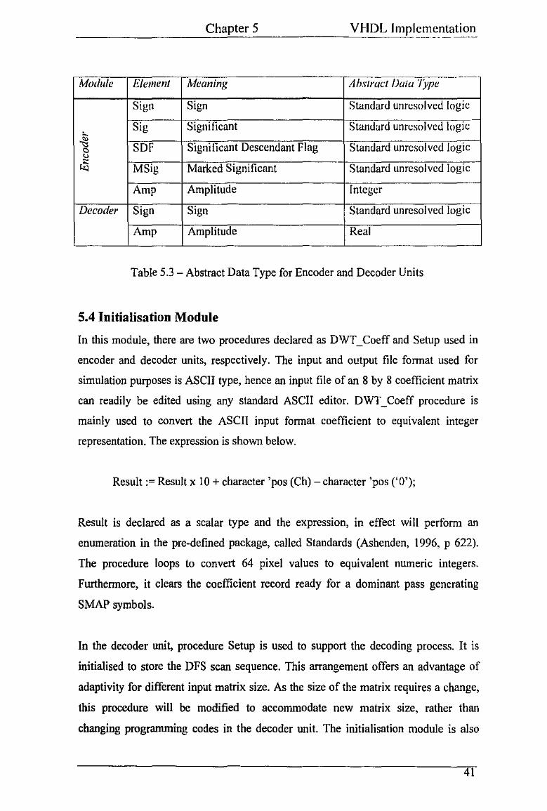
________ ____:cCcchc:ap"-t:..:e:..r:..S ______ _cV_c.~:.ciD=-L=-Implc~l11~ntatioll_
Module Element Meaning Ah.\·trlict7JUiu.l'ype~------·
Sign Sign Standard unresolved logic
~ Sig Significant Standard unresolved logic
SDF Significant Descendant Flag Standard unresolved logic c " <:\ MSig Marked Significant Standard unresolved logic
Amp Amplitude Integer
Decoder Sign Sign Standard unresolved logic
Amp Amplitude Real
Table 5.3- Abstract Data Type for Encoder and Decoder Units
5.4 Initialisation Module
In this module, there are two procedures declared as DWT _ Coeff and Setup used in
encoder and decoder units, respectively. The input and output file format used for
simulation purposes is ASCII type, hence an input file of an 8 by 8 coefficient matrix
can readily be edited using any standard ASCII editor. DWT _ Coeff procedure is
mainly used to convert the ASCII input format coefficient to equivalent integer
representation. The expression is shown below.
Result:~ Result x IO +character 'pos (Ch)- character 'pos ('0');
Result is declared as a scalar type and the expression, in effect will perform an
enumeration in the pre~defined package, called Standards (Ashenden, 1996, p 622).
The procedure loops to convert 64 pixel values to equivalent numeric integers.
Furthermore, it clears the coefficient record ready for a dominant pass generating
SMAP symbols.
In the decoder unit, procedure Setup is used to support the decoding process. It is
initialised to store the DFS scan sequence. This arrangement offers an advantage of
adaptivity for different input matrix size. As the size of the matrix requires a change,
this procedure will be modified to accommodate new matrix size, rather than
changing programming codes in the decoder unit. The initialisation module is also
41
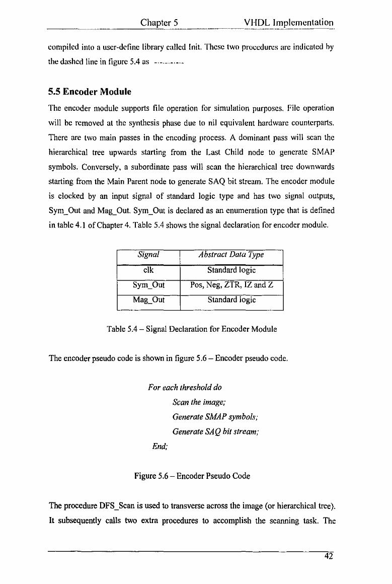
compiled into a user-define library called I nit. These two proccdun:s arc indicated by
the dashed line in figure 5.4 as -·-·-·-·-·-
5.5 Encoder Module
The encoder module ~upports file operation for simulation purposes. File operation
will be removed at the synthesis phase due to nil equivalent hardware counterparts.
There are two main passes in the encoding process. A dominant pass will scan the
hierarchical tree upwards starting from the Last Child node to generate SMAP
symbols. Conversely. a subordinate pass will scan the hierarchical tree downwards
starting from the Main Parent node to generate SAQ bit stream. The encoder module
is clocked by an input signal of standard logic type and has two signal outputs,
Sym_Out and Mag_ Out. Sym_Out is declared as an enumeration type that is defined
in table 4.1 of Chapter 4. Table 5.4 shows the signal declaration for encoder module.
Signal Abstract Data Type
elk Standard logic
Sym_Out Pos, Neg, ZTR, IZ and Z
Mag_ Out Standard logic
Table 5.4- Signal Declaration for Encoder Module
The encoder pseudo code is shown in figure 5.6- Encoder pseudo code.
For each threshold do
End;
Scan the image;
Generate SMAP symbols;
Generate SAQ bit stream;
Figure 5.6- Encoder Pseudo Code
The procedure DFS_Scan is used to transverse across the image (or hierarchical tree).
It subsequently calls two extra procedures to accomplish the scanning task. The
42

Chapter 5 VI-IDL Implementation
coefticient has determined its status of significance in a procedure called Compare.
The initial coefficient values are kept in an array of 64 clements. These cocflicicnt
values arc compared and the SMAP symbols arc generated in a procedure named
Sym _Gen. However to generate the SAQ bit stream, a coefficient whose record
element of MSig is set is compared with the current threshold and corresponding
width in procedure named Mag_ Gen. Should the coefficient value be within the upper
half of the width, a I symbol is sent out, otherwise a 0 symbol is sent out (that is
within the lower half of the width). These procedures are executed until the bit budget
is exhausted or the transmission is terminated as a pre-determined condition of
distortion measure is reached.
5.6 Decoder Module
The scan sequence for the decoder module is stored in the initialisation module. It is a
modular design. Hence it is relatively simple to modify should a different matrix size
be used. The initialisation module can be modified without affecting the decoder
module. In the decoder module, two separate procedures are utilised to process SMAP
and SAQ streams. A procedure called Decode_SMAP is used to decipher the SMAP
symbols. Consequently, it calls second procedure; Process_ Symbol to process each
symbol individually. Process_Symbol can initiate an appropriate jump for the ZTR
symbol. To decipher the SAQ bit stream; procedure of Dec~de _ SAQ is used. The
computation is based on the expressions presented in chapter 4 - EZW algorithm.
Finally, a procedure named Display_Result is used to output the reconstructed data.
The merit of clocking for the decoder module has a similarity to the encoder module.
That is the decoder module can be clocked by an internal or external clock source.
The intemaVextemal clocking decision mainly depends on the encoder/decoder as a
stand-alone module or incorporated into a larger VLSI with DWT module. The
decoder pseudo code is shown in figure 5. 7 - Decoder pseudo code.
Initialise;
For each threshold do
Decode SMAP symbols;
Decode SAQ bit stream;
End;
Figure 5.7- Decoder Pseudo Code
43
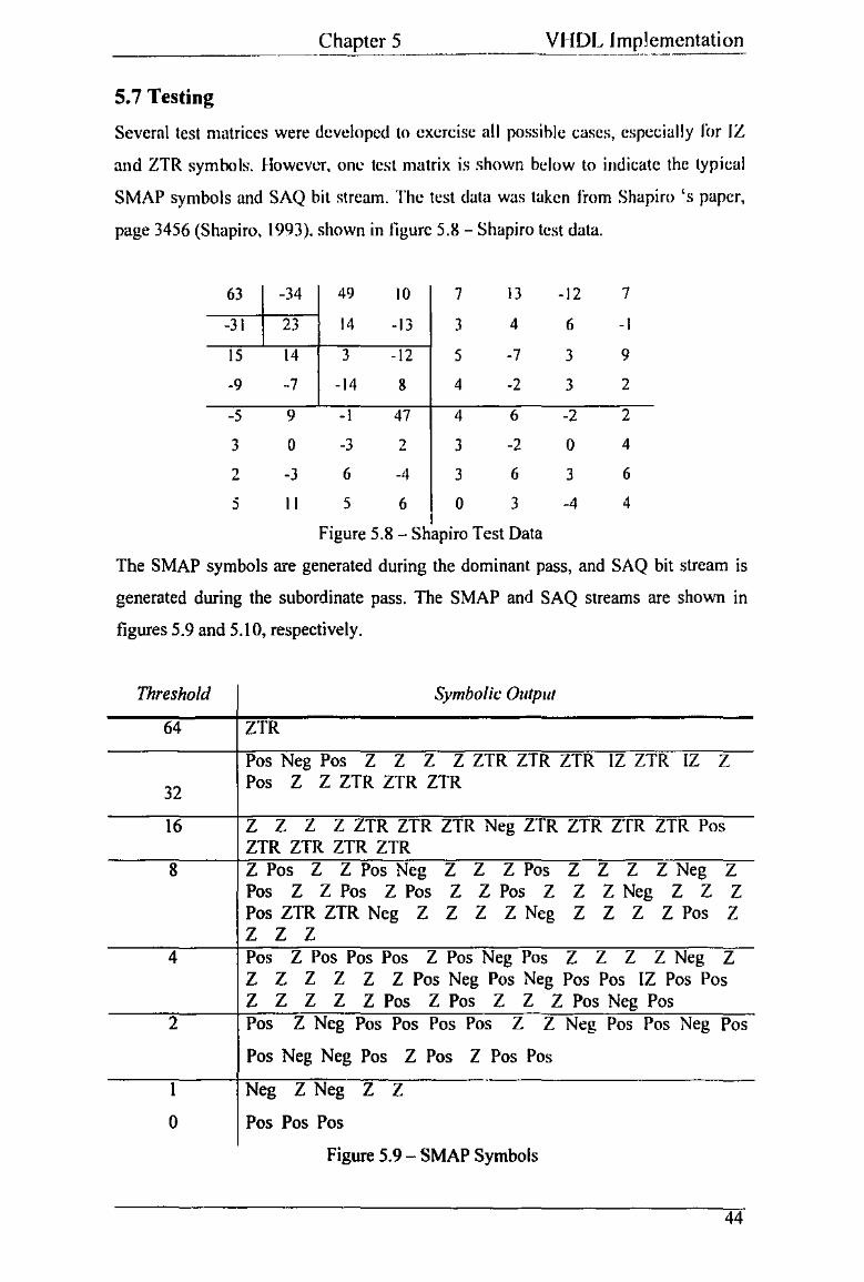
5.7 Testing
Several test matrices were developed to exercise all possible cases, especially for IZ
and ZTR symbols. However, one test matrix is shown below to indicate the typical
SMAP symbols and SAQ bit stream. The test data was taken from Shapiro 's paper,
page 3456 (Shapiro, 1993). shown in figure 5.8- Shapiro test data.
63 -34 49 10 7 13 -12 7
-31 23 14 -13 3 4 6 -I
15 14 3 -12 5 -7 3 9
-9 -7 -14 8 4 -2 3 2
-5 9 -I 47 4 6 -2 2
3 0 -3 2 3 -2 0 4
2 -3 6 -4 3 6 3 6
5 II 5 6 0 3 -4 4
Figure 5.8- Shapiro Test Data
The SMAP symbols are generated during the dominant pass, and SAQ bit stream is
generated during the subordinate pass. The SMAP and SAQ streams are sho"'n in
ligures 5.9 and 5.10, respectively.
Threshold
64
32
Symbolic Output
ZTR
Pos Neg Pos Z Z Z Z ZTR ZTR ZTR IZ ZTR lZ Z Pos Z Z ZTR ZTR ZTR
16 Z Z Z Z ZTR ZTR ZTR Neg ZTR ZTR ZTR ZTR Pos ZTR ZTR ZTR ZTR
8 Z Pos Z Z Pos Neg Z Z Z Pos Z Z Z Z Neg Z Pos Z ZPos ZPos Z ZPos Z Z ZNeg Z Z Z Pos ZTR ZTR Neg Z Z Z Z Neg Z Z Z Z Pos Z z z z
4 Pos Z Pos Pos Pos Z Pos Neg Pos Z Z Z Z Neg Z Z Z Z Z Z Z Pos Neg Pos Neg Pos Pos IZ Pos Pos Z Z Z Z ZPos ZPos Z Z ZPosNegPos
2 Pos Z Neg Pos Pos Pos Pos Z Z Neg Pos Pos Neg Pos
Pos Neg Neg Pos Z Pos Z Pos Pos
I Neg Z Neg Z Z
0 Pos Pos Pos
Figure 5.9- SMAP Symbols
44

Chapter 5 VHDL Implementation
Thresholcl Magnitude Output
64 ---
32 I 0 I 0
16 I 0 0 I I 0
8 I 0 0 I I I I 0 0 I 1010100010
4 I 0 0 I I I 0 0 I 0 0 0 I 0 0 0 I I 0 I I 0
I 0 0 I 0 0 0 I 0 0 0 0 0 0 0 0 0 0 0
2 0 I 0 0 0 0 0 I I I 0 0 0 0 I 0 0 I I I 0 I
0 I 0 0 I 0 0 0 I I 0 I I I I I I I I 0 0 0
0 0 0 0 0 0 0 0 0 0 0 0 0 0 0
I 0 I 000001 I I 0 0 0 0 I 0 0 I I 1 0 I 0 I 0 0 I 0 0 0 I I 0 1 1 I I I I I I 0 I 0 0 I 0 0 I I 0 0 0 I I I 0 0 0 0 0
0 0 I 0 0 0 0 0 1 I I 0 0 0 0 1 0 0 I 1 1 0 I 0 I 0 0 I 0 0 0 I I 0 I I I I I I I 1 0 I 0 0 I 0 0 I I 0 0 0 I I 1000001 0 I
Figure 5.10- SAQ Bit Stream
The two streams are deciphered at the decoder module, and the reconstructed data is
presented in figure 5.11 -Reconstructed data, shown below.
63 -33 49 9 7 13 -II 7
-31 23 13 -13 2 5 5 -I
IS 13 2 -II 5 -7 2 9
-9 -7 -13 II 5 -2 2 2
-5 9 -I 47 5 5 -2 2
2 0 -2 2 2 -2 0 5
2 -2 5 -5 2 5 2 5
5 II 5 5 0 2 -5 5
Figure 5.11 -Reconstructed Data
45
-

Chapter 6 - Simulation Result
In this chapter, the EZW DFS algorithm derived and implemented in previous
chapters will be tested using real image such Lenna. The aspect of embedded
transmission is also examined closely by terminating the transmission at certain
thresholds. So the distortion measure can be computed to evaluate the effectiveness of
the proposed algorithm. The chapter first studies a short history of Lenna image. Next,
a number of incomplete l!mbedded transmissions will be tested and their distortion
metric will be compared. At the conclusion of the chapter, a summary of distortion
will be produced for comparison purposes.
6.1 Leona- Who was she?
Many worldwide researchers and students working in image processing would be
likely to use the image of the mysterious Lenna in their work. But who was Lenna and
how was it started with her as an image model? The humble answer could be traced
back to the November, I 972 issue of Playboy magazine, a Swedish centrefold model
named Lena Soderberg (Lenna is the English spelling in Playboy magazine) was
scanned by research student at the time; Dr. William K. Pratt for his study of image
processing. Since, the image of Lenna has been practically adapted as standard test
image for comparison purposes by many image-processing professionals.
Finally, Lenna was invited to attend the 50th Anniversary of Image Science and
Technology in Boston on May !997. She was amazed at how her image could
contribute to advance modern science over the past many years. Lenna commented to
the reporters that "They must be so tired of me ... looking at the same picture for all
these years!".
Currently, Lenna lives near Stockholm and works for a govenunent agency
supervising handicapped employees archiving data using computers and scanners.
Without any doub~ Lenna image is the most widely used test image nowadays (Po,
1997).
46
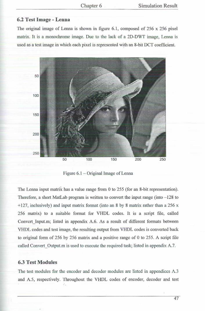
Chapter 6 Simulation Result
6.2 Test Image - Lenna
The original image of Lerma is shown in figure 6.1, composed of 256 x 256 pixel
matrix. It is a monochrome image. Due to the lack of a 2D-DWT image, Lerma is
used as a test image in which each pixel is represented with an 8-bit DCT coefficient.
50
100
150
Figure 6.1 - Original Image of Lerma
The Lerma input matriX has a value range from 0 to 255 (for an 8-bit representation).
Therefore, a short MatLab program is written to convert the input range (into - 128 to
+ 127, inclusively) and input matrix format (into an 8 by 8 matrix rather than a 256 x
256 matrix) to a suitable format for VHDL codes. It is a script file, called
Convert_Input.m; listed in appendix A.6. As a result of different formats between
VHDL codes and test image, the resulting output from VHDL codes is converted back
to original form of 256 by 256 matrix and a positive range of 0 to 255. A script file
called Convert_ Output.m is used to execute the required task; listed in appendix A. 7.
6.3 Test Modules
The test modules for the encoder and decoder modules are listed in appendices A.3
and A.5, respectively. Throughout the VHDL codes of encoder, decoder and test
47
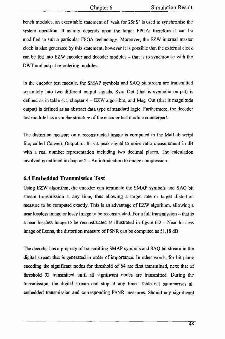
Chapter 6 Simulation Result
bench modules, an executable statement of 'wait for 25nS' is used to synchronise the
system operation. It mainly depends upon the target FPUA; therefore it can be
modified to suit a particular FPGA technology. Moreover, the EZW internal master
clock is also generated by this statement, however it is possible that the external clock
can be fed into EZW encoder and decoder modules- that is to synchronise with the
DWT and output re-ordering modules.
In the encoder test module, the SMAP symbols and SAQ bit stream are transmitted
sl"parately into two different output signals. Sym_Out (that is symbolic output) is
defined as in table 4.1, chapter 4- EZW algorithm, and Mag_ Out (that is magnitude
output) is defined as an abstract data type of standard logic. Furthermore, the decoder
test module has a similar structure of the encoder test module counterpart.
The distortion measure on a reconstructed image is computed in the MatLab script
file; called Convert_Output.m. It is a peak signal to noise ratio measurement in dB
with a real number representation including two decimal places. The calculation
involved is outlined in chapter 2- An introduction to image compression.
6.4 Embedded Transmission Test
Using EZW algorithm, the encoder can terminate the SMAP symbols and SAQ bit
stream transmission at any time, thus allowing a target rate or target distortion
measure to be computed exactly. This is an advantage of EZW algorithm, allowing a
near lossless image or lossy image to be reconstructed. For a full transmission- that is
a near lossless image to be reconstructed as illustrated in figure 6.2 - Near lossless
image ofLenna, the distortion measure ofPSNR can be computed as 51.18 dB.
The decoder has a property of transmitting SMAP symbols and SAQ bit stream in the
digital stream that is generated in order of importance. In other words, for bit plane
encoding the significant nodes for threshold of 64 are first transmitted, next that of
threshold 32 transmitted until all significant nodes are transmitted. During the
transmission, the digital stream can stop at any time. Table 6.1 summarises all
embedded transmission and corresponding PSNR measures. Should any significant
48
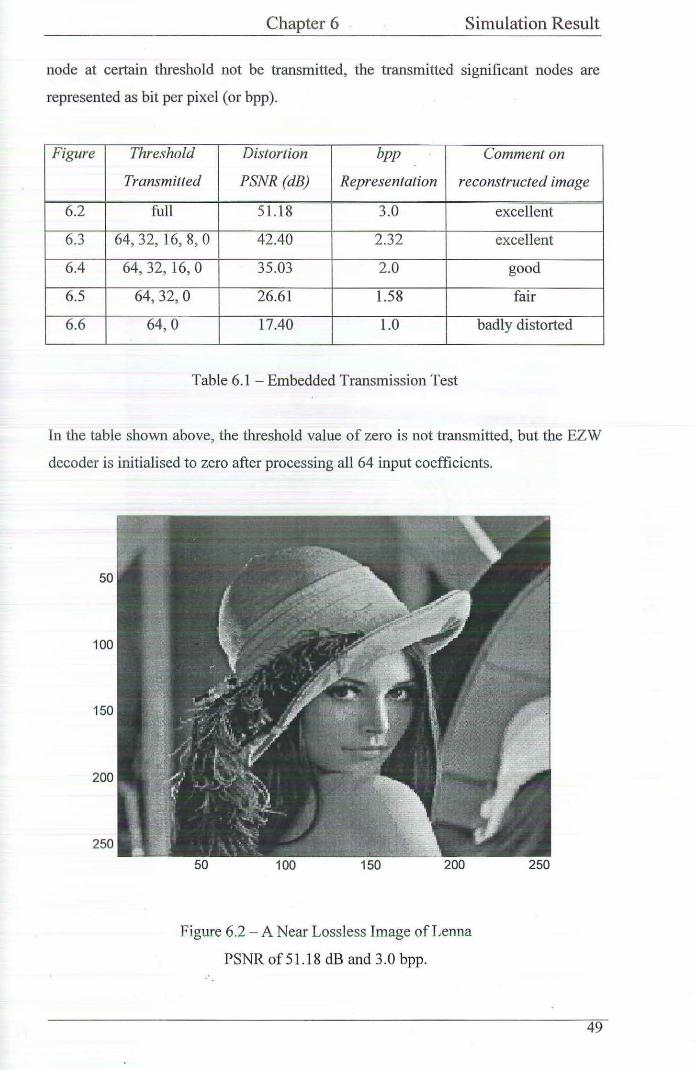
Chapter 6 Simulation Result
node at certain threshold not be transmitted, the transmitted significant nodes are
represented as bit per pixel (or bpp ).
Figure Threshold Distortion bpp Comment on
Transmitted PSNR (dB) Representation reconstructed image
6.2 full 51.18 3.0 excellent
6.3 64, 32, 16, 8,0 42.40 2.32 excellent
6.4 64,32, 16, 0 35.03 2.0 good
6.5 64,32,0 26.61 1.58 fair
6.6 64, 0 17.40 1.0 badly distorted
Table 6.1 - Embedded Transmission Test
In the table shown above, the threshold value of zero is not transmitted, but the EZW
decoder is initialised to zero after processing all 64 input coefficients.
100 150
Figure 6.2- A Near Lossless Image ofLenna
PSNR of51.18 dB and 3.0 bpp.
49

50
100
150
200
250
Chapter 6
Figure 6.3- Lossy Image ofLenna
PSNR of 42.40 dB and 2.32 bpp.
Simulation Result
50
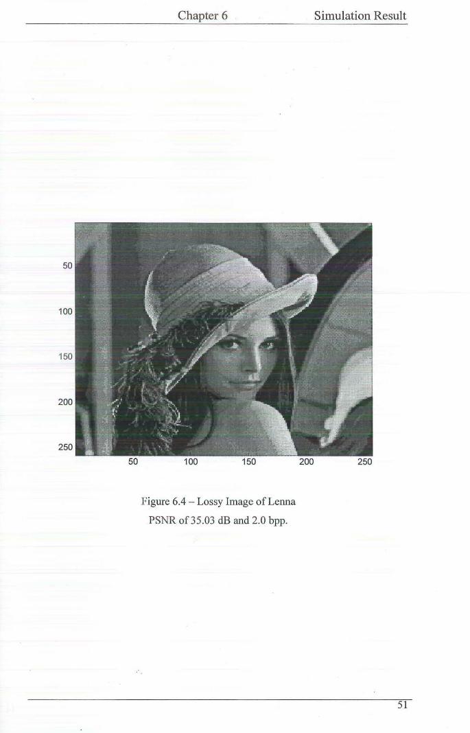
50
100
150
200
250
50
Chapter 6
100 150
Figure 6.4 - Lossy Image of Lenna
PSNR of 35.03 dB and 2.0 bpp.
··.
Simulation Result
200 250
51
50
100
150
. ·
Chapter 6
Figure 6.5 - Lossy Image ofLenna
PSNR of26.61 dB and 1.58 bpp .
Simulation Result
52
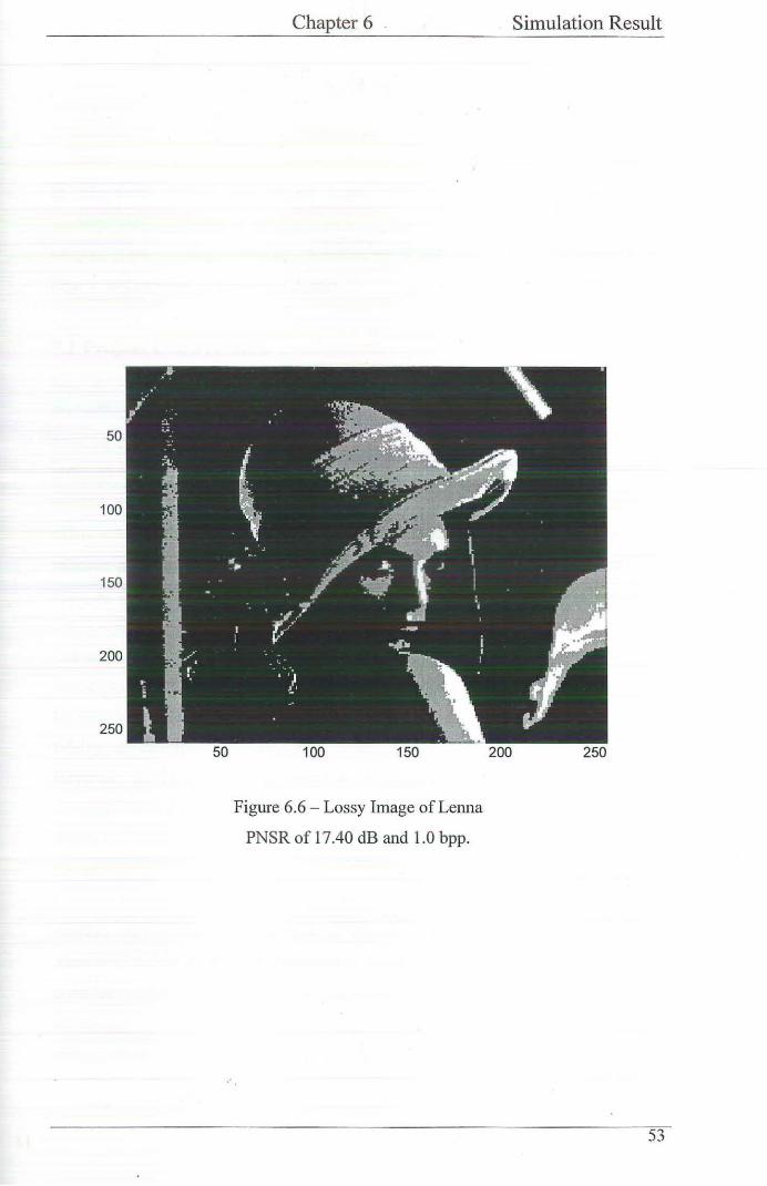
50
100
150
200
250
50
Chapter 6
100 150
Figure 6.6 - Lossy Image ofLenna
PNSR of 17.40 dB and 1.0 bpp.
Simulation Result
200 250
53
Chapter 7 - Conclusion
In this final chapter, the project contribution will detail many maJOr tasks
accomplished; including a practical focus of mastering the Peak-VHDL PC-based
version. It also highlights a further direction and a wish list to be accomplished if the
time would othetwise be made available.
7.1 Project Contribution
One of the most significant contributions of this project is to be able to simulate the
Embedded Zerotree Wavelet algorithm, first proposed by Jerome M. Shapiro in 1993.
Most of the suggested details discussed in Shapiro 's paper is derived and extended,
although the derived and implemented algorithm is based on the Depth First Search
method rather than the Breadth First Search method - However, the DFS method
offers a better solution compared to the BFS method. As the EZW DFS algorithm
requires minimum storage in EZW processor, its processing speed is expected to
increase. As a result, the EZW processor architecture will be simpler to implement.
The second significant contribution is to be able to obtain near-lossless reconstructed
image. As the Significance Map symbols and Successive Approximation Quantisation
bit stream are allowed to be fully transmitted, the reconstructed image will have high
fidelity; the distortion measure of Peak Signal to Noise Ratio is in the order of 50 dB.
However, should the stopping condition be reached (a target bit rate or distortion
measure is exactly met), the reconstructed image is reasonably recognisable as many
details can clearly be differentiated; the distortion measure of PSNR is in the order of
20dB.
Another contribution is to be able to present a conctse explanation of wavelet
transform teclmique from an engineering point of view without utilising to many
complex mathematical expressions. However, a number of equations are also
introduced to aid a further understanding on such a complex topic. Furthermore, such
mathematical equations can be realised by using a set of high pass and low pass
54
Chapter 7 Conclusion
filters. Consequently. the merit of this realisation can be applied to the EZW
algorithm.
The main focus of this project is to simulate the EZW algorithm in l'cak-VHDL PC
based environment. The Peak VHDL software was used extensively throughout the
project. It provides an economical tool to accomplish the set out goals compared to
main frame computers such Unix. Although DCT technique is used to present the
original test image of Leona, the EZW DFS algorithm is tested on a black box basis.
Therefore, we are highly confident that should the discrete wavelet transform be
available, more spectacular results would be obtained.
7.2 Further Direction
Due to time constraint, the following wish list in the selected order could otherwise be
fulfilled
The scan sequence for an 8 by 8 matrix was incorporated in the VHDL encoder
codes. However, it should be written in a separate module, thus the algorithm is
truly modular. This will offer an advantage of modular adaptivity for different
input matrix size. As discussed in chapter 4 - EZW algorithm, the validity of
zerotree data structure mainly depends upon the analysis window, which is the
input matrix size. Therefore, it is less likely that the zerotree hypothesis is violated
- more efficient compression EZW algoritlun can offer. The above discussion
only applies to the encoder module.
The input/output file format is ASCII type. However, to minimise the storage
space for files, the input/output file should be kept in binary format. Yet, the
binary file format is mainly software-vendor dependent. This requires time to
correspond with the software vendor. Furthermore, it also depends on software
vendor after-sale support.
20-DWT coefficients should be used to utilise the full strength of EZW algorithm.
It is expected that the results will be more spectacular. Although DCT coefficients
were used, the results of near loss!ess (PSNR is 51 dB) to a lossy reconstructed
image (PSNR is 35 dB or 2 bits per pixel) are a reasonable achievement.
The implemented algorithm should be synthesised and tested at a hardware level.
The timing issue could be encountered and changes could consequently be made
55

Chapter 7 Conclusion
on the proposed architecture. Peak FPGA software is such an excellent tool fOr
fast prototyping.
Finally, this project provides a good opportunity for further work by building on an
existing gained knowledge as listed below.
An adaptive arithmetic encoder can be derived and implemented as suggested in
chapter 4- EZW algorithm. It is possible to achieve an image compression having
the distortion measure in the order of 40 dB or I bit per pixel.
The ultimate challenge could be asked as 'How eco!lomically to stop the
embedded transmission provided the reconstructed image is reasonably
recognisable' or 'What is the best universal compression ratio for any image?'.
The task could be fulfilled by carrying out a series of tests on different images.
However, a knowledge of different techniques/fields will be required to gain, such
edge detection, pattern recognition and the like in order to accomplish further
work. This is an ultimate step that can be taken to further promote the work in this
project.
56

Bibliography
[1] Ang L., Cheung H. N. & Eshraghian K. (1999). EZW Algorithm Using
Depth-First Search Representation of the Wavelet Zerotree. Proceedings 5th
International Symposium on Signal Processing and Its Applications, pp. 75 -
78.
[2] Ang L., Cheung H. N. & Eshraghian K. (1999). VLSl Architecture for
Embedded Zerotree Wavelet Coding. Proceedings 5th International
Symposium for Communication Systems, pp. 128- 133.
[3] Antonini M., Barlaud M., Mathieu P. & Daubechies I. (1992). Image Coding
Using Wavelet Transform. IEEE Transactions on Image Processing. Vol 1
(2).
[4] Ashenden, P. (1996). The Designer's Guide to VHDL. California: Morgan
Kaufmann Publishers, Inc.
[5] Barlaud, M. (1994). Wavelets m Image Communication. Amsterdam:
Elsevier Science B. V.
[6] Chang, K. C. (1997). Digital Design and Modeling With VHDL and
Synthesis. California: IEEE Computer Society Press.
[7] Cheung C. H., Wang S. Y., Cheung K. W. & Po L. M. (1999). Embedded
Lossless Wavelet Coder Using Multi-Partitioning Algorithm. Proceedings
14th International Conference on Computers and Their Applications.
[8] Clarke, R. J. (1993). A Survey of Low-Rate Digital Image Coding
Techniques. Canadian Conference on Electrical and Computer Engineering.
Vol!, pp. 27-30.
[9] Clarke, R.J. (1993). A Survey of Low Rate Digital Image Coding
Techniques. Canadian Conference on Electrical and Computer Engineering.
Vol!, pp. 27-30.
[10] Creusere, C. D. (1997). A New Method of Robust Image Compression Based
on the Embedded Zerotree Wavelet Algorithm. IEEE Transactions on Image
Processing. Vol6 (10), pp. 1436- 1442.
[II] Gander, W., & Hrebicek, J. (1995). Solving Problems in Scientific
Computing Using Maple and MatLab. (2"' exp. ed.). New York: Springer.
[12] Gonzalez, R. C. & Woods, R. E. (I 993). Digital Image Processing.
57

Massachusetts: Addison- Wesley Publishing Company.
[JJJ Green. W. (1989). Digit~!)mJ_lge Pr~~c_,.:s~I!llL~ A.~yst~ms Approach. (2m1 cd.).
New York: Van Nostrand Reinhold.
[14] IEEE Standard VHDL Language Reference Manual. (Available from the
Institute of Electrical ami Electronic Engineers, Inc. 345 East 47'11 Street,
New York. NY 10017. USA)
[IS] Lewis A. S. & Knowles Ci. ( 1992). Image Compression Using the 2-D
Wavelet Transform. IEEE transactions on Image Processing. Vol 1 (2).
[16] Martucci S. A., Sodagar 1., Chiang T. & Zhang Y. Q. (1997). A Zerotree
Wavelet Video Coder. IEEE Transactions on Circuits and Systems for Video
Technology. Yol7 (1), pp. 109-118.
[17] Mathews, J. H., & Fink, K. D. (1999). Numerical Methods Using MatLab (3''
ed.). New Jersey: Prentice Hall.
[18] Meyer, Y. (1993). Wavelets: Algorithm and Applications. Philadelphia:
Society for Industrial and Applied Mathematics.
[19] Navabi, z. (1993). VHDL Analysis and Modeling of Digital Systems. New
Jersey: Me Graw Hill.
[20] Netravali, A. N. & Haskell, G. B. (1989). Digital Pictures- Representation
and Compression. New York: Plenum Press.
[21] 0 'Neil, P. (1995). Advanced Engineering Mathematics (41h ed.).
Massachusetts: PWS Publishing Company.
[22] Parker, J. R. (1997). Algorithnns for Image Processing and Computer Vision.
New York: John Wiley & Sons, Inc.
[23] Peak VHDL User 's Guide - Professional Edition. (Available from Protei
Technology, Inc. 5252 North Edgewood Drive, Suite 175. Provo. UT 84604.
USA)
[24] Po, L. M. (1997). A Complete Story of Lenna. [on-line]. Available WWW:
http://www.image.cityu.edu.hk
[25] Polikar, R. (1994). The Wavelet Tutorial. [on-line]. Available WWW:
http://www.public.iastate.edu/-rpolikar/W A VELETS.
[26] Prasanna, V. K. & Bae, J. (1995). A Fast and Area-Efficient YLSI
Architecture for Embedded Image Coding. Proceedings International
Confere .. ce on Image Processing. Vol3, pp. 452-455.
58
[27] Said, A. & Pearlman, W. (1996). A New, Fast, and Efficient Image Codcc
Based on Set Partitioning in Hierarchical Trees. IEEE Transactions on
Circuits and Systems for Video Technology. Vol 6 (3), pp. 243-250.
[28] Shapiro, J.M. (1993). Embedded Image Coding Using Zerotrces of Wavelet
Coefficients. IEEE Transactions on Signal Processing. Vol 41 (12), pp. 3445
-3462.
[29] Sigmon, K. (1994). MatLab Primer (41h ed.). Florida: CRC Press.
[30] Thornton, S. T., & Rex, A. (1993). Modern Physics for Scientists and
Engineers. Florida: Saunder College Publishing.
[31] Topiwala, P. N. (1998). Wavelet Image and Video Coding. Massachusetts:
Kluwer Academic Press.
[32] Valens, C. (!999). EZW Encoding. [on-line]. Available WWW:
http://perso.wanadoo.fr/polyvalens/clemens/ezw/ezw.html.
[33] Vetterli, M., & Kovacevic, J. (1995). Wavelets and Subband Coding. New
Jersey: Prentice Hall.
[34] VHDL Forum. (2000). [on-line]. Available WWW: http:/www.vhdl.org/.
[35] Wade, G. (1994). Signal Coding and Processing. (2"' ed.). Cambridge:
Cambridge University Press.
[36] Young, R. K. (1993). Wavelet Theory and Its Applications. Massachusetts:
Kluwer Academic Press.
59

Appendices

Listing A.O Support. vhd
Global declaration Written by Hung !luynh Hierarchical level 0
library IEEE:;
use IEEE.std_logic_ll64.all;
package Type Def is
64) ;
type Code_Type is {Pas, Neg, IZ, Z'l'R, Z); type Array Length is array ( 0 to 7) of integer;
constant Thres_Array : Array_Length := (0 1 1, 2, 4, 8, 16, 32,
constant Image_Size : integer := 1023; constant Stack_Length : integer := 63;
type Coeff Rec is -- Elemental unit in coding record
Sign Sig SDF MSig Amp
end record; type Index Info is
record
std_ulogic; std_ulogic; -- Significant bit std_ulogic; std_ulogic; integer;
Used to store the scan sequence
Index No : integer; SAQ_Counter : integer; Done : boolean;
end record; type Coeff Det is -- Elemental unit in decoding
record Sign : std_ulogic; Amp real;
end record;
type Stack_Type is array (0 to Stack Length) of Coeff Rec; type Scan_Index_Type is array (0 to Stack_Length) of
Index Info; type Storage_Type is array (0 to Stack_Length) of Coeff Det; type DWT_Type is array (0 to Stack_Length) of integer;
end Type_Def;
61

Listing A. I lnit.vhd
IO Operation Written by Hung Huynh Hierarchical level 1
library IEEE, std, support;
use IEEE.std_logic_ll64.all,
package Loaded_File is
std. textio.all, support.Type_Def.all;
procedure DWT Coeff (DWT: DWT_Type; Stack Ln : line; Index : integer); end Loaded File;
use IEEE.std_logic_1164.all, support.Type_Def.all;
package Decode !nit is
Stack_Type;
procedure Setup (Storage Scan_Index_Type);
Storage_Type; Scan_Index
end Decode !nit;
package body Loaded_File is
procedure DWT_Coeff (OWT : inout DWT_Type; Stack Stack_Type; Ln : in line; Index : inout integer) is
in out
-- This procedure is used to convert ASCII code to decimal value for input coefficients
begin
variable Ch : character; variable Neg_Flag : boolean := false; variable Result : integer := 0;
for Count! in 0 to 7 loop for Count2 in 0 to 3 loop
read (Ln, Ch); if Ch I= ' ' then
if Ch = '-' then Neg_Flag := true;
else Result := Result * 10 +
character'pos (Ch) - character'pos ('0'); end if;
end if; end loop; if Neg_Flag then
Result := - Result; end if; DWT (Index) := Result; Index := Index + 1; Result := 0; Neg_Flag :~ false; read (Ln, Ch);
end loop; for Count! in 0 to Stack_Length loop
Stack(Countl).Sign :~ '-';
62
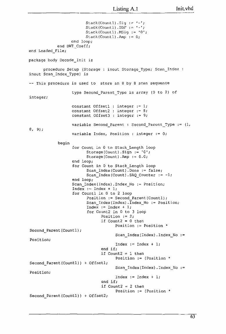
Listing A.l Jnit.vhd
Stack(Countl) .Siq- !"'" '-';
Stack (Count 1) . [~DE' : ~ '-';
Stack(Countl) .MSiq :~ '0'; St:acJ.:(Countl) .Amp :~ 0;
end loop; end DWT_ Coe f f;
end Loaded ~ile;
package body Decode_Init is
procedure Setup (Storage inout Scan_Index_Type) is
inout Storage_Type; Scan Index.
-- This procedure is used to store an 8 by 8 scan sequence
integer;
8, 9);
begin
type Second Parent_Type is array (0 to 2) of
constant Offset! constant Offset2 constant Offset3
integer integer integer
;= 1 i ;= 8 i := 9;
variable Second Parent : Second Parent_Type := (1,
variable Index, Position : integer := 0;
for Count in 0 to Stack_Length loop Storage(Count) .Sign := '0'; Storage(Count) .Amp := 0.0;
end loop; for Count in 0 to Stack_Length loop
Scan_Index(Count) .Done ;; false; Scan_Index(Count).SAQ_Counter := -1;
end loop; Scan_Index(Index) .Index_No := Position; Index := Index + 1; for Count1 in 0 to 2 loop
Position := Second_Parent(Count1); Scan_Index(Index) .Index_No := Position; Index := Index + 1; for Count2 in 0 to 3 loop
Position : = 2; if Count2 = 0 then
Position := Position * Second_Parent(Count1);
Position; Scan_Index{Index) .Index_No :=
Index := Index + 1; end if; if Count2 = 1 then
Position := {Position * Second_Parent(Count1)) +Offset!;
Position; Scan_Index(Index) .Index_No :=
Index := Index + 1; end if; if Count2 = 2 then
Position := (Position * Second_Parent(Countl)) + Offset2;
63

Position;
Listing A. I lnit.vhd
Scan Ind(~;.: (Index). Index Ho :""
Index :"" Tndex -l 1; end i [; if Count2 = 3 then
Position := (Position ~
Second_Parent (Countl)) + Offset3;
Position; Scan Index(Indl'n:) .Ind-::x_No :=
Index := Index + 1; end .if; Position := Position 1 2; Scan_Index (Index). Index_No := Position; Index := Index + 1; Position := Position + 1; Scan_Index(Index) .Index_No := Position; Index := Index + 1; Position := Position + 7; Scan_Index(Index) .Index_No :=Position; Index := Index + 1; Position := Position + 1; Scan_Index(Index) .Index_No :=Position; Index := Index + 1;
end loop; end loop;
end Setup; end Decode Init;
64
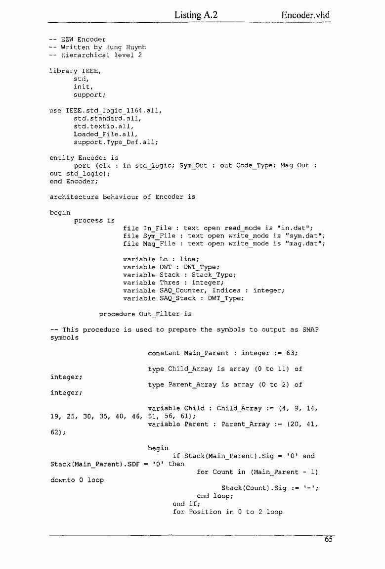
Listing A.2 Encoder. vhd
EZW Encoder Written by Hung Huynh Hierarchical level 2
library IEEE, std, in it, support;
use IEEE.std_logic_l164.all, std.standard.all, std.textio.all, Loaded_File.all, support.Type Def.all;
entity Encoder is port (elk in std_logic; Sym_Out
out std_logic); out Code_Type; t<lag_Out
end Encoder;
architecture behaviour of Encoder is
begin process is
file In_File : text open read_mode is "in.dat"; file Syrn_File text open write mode is "sym.dat"; file Mag_File : text open write mode is "mag.dat";
variable Ln : line; variable DWT : DWT_Type; variabl& Stack : Stack_Type; variable Thres : integer; variable SAQ_Counter, Indices integer; variable SAQ_Stack : DWT_Type;
procedure Out_Filter is
-- This procedure is used to prepare the symbols to output as SMAP symbols
constant Main_Parent : integer := 63;
type Child_Array is array (0 to 11) of integer;
type Parent_Array is array (0 to 2) of integer;
variable Child : Child_Array := (4, 9, 14, 19, 25, 30, 35, 40, 46, 51, 56, 61);
variable Parent : Parent_Array := (20, 41, 62);
begin if Stack(Main_Parent) .Sig = '0' and
Stack(Main_Parent) .SDF = '0' then
downto 0 loop for Count in (Main_Parent - 1)
Stack(Count) .Sig := '-'; end loop;
end if; for Position in 0 to 2 loop
65

Listing A.2 Encodcr.vhd
if Stack(Parent(Position)) .Si1 '0' and Stack(Parent(Position)) .SDF = '0' thon
for Count in 0 to 19 loop
Stack(Parent(Position) - 1 -Count) .SDF :m '-';
Stack(Parent(Position) - l - Count).Sig := end
·-'. '
'1' then
end if; end loop;
loop;
for Po3i tion in 0 to 11 loop if Stack(Child(Position)) .Sig
for Count in 0 to 3 loop Stack(Child(Position}
- 1- Count) .SDF := 'L'; end loop;
end if; end loop; for Position in 0 to 11 loop
if Stack(Child(Position)) .Sig '0' and Stack(Child(Position)) .SDF = '0' then
for Count in 0 to 3 loop Stack(Child(Position)
- 1 - Count) .SDF := '-';
integer) is
end loop; end if;
end loop; end Out Filter;
procedure Subband (Index : in integer; Band Num
-- This procedure is used to locate the decomposed subband
constant HL constant LH constant HH
integer integer integer
:= 4 2; := 21; := 0;
begin if Index = 31 then
Band Num : = HL; e1sif Index = 59 then
Band_Num := LH; elsif Index = 63 then
Band Num : = HH; end if;
end Subband;
inout
procedure Compare (Index, Thres inout boolean; Band_Num : inout integer) is
in integer; Sig_Flag
-- This procedure is used to test coefficient against the current threshold
begin if Stack(Band_Num) .MSig /= '1' and Thres /= 0
then if (abs(DWT(Index)) > Thres) then
Stack(Band_Num) .Sig := '1';
66
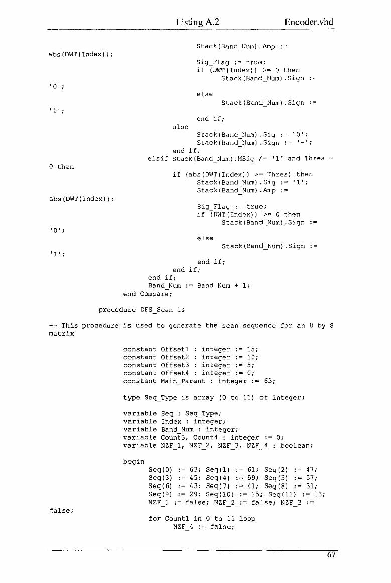
abs (DWT (Tndex));
'0';
I ' I ,
" '
0 then
abs(DWT(Index));
I 0 I j
I 1 I j
Listing A.2 Encoder. vhd
else
---.--·
Stack(Band Num) .Amp :'""
Sig_Flag :~ true; i[ (D\o'l'l'(Indez)) >eo 0 then
Stack(Band_Nurn) .Sign :=
else Stack (Band_Nurn) .Sign :=
end if;
Stack (Band _Num) . Sig : = '0'; Stack(Band_Num) .Sign := '-';
end if; elsif Stack(Band_Num) .MSig /= '1' and Thres
if (abs(OfriT(Index)) >= Thres) then Stack(Band_Num) .Sig := '1'; Stack(Band_Num) .Amp :=
Sig_Flag := true; if {DWT(Index)) >= 0 then
Stack(Band_Num),.Sign :=
else Stack(Band_Num) .Sign :=
end if; end if;
end if; Band Num := Band Num + 1;
end Compare;
procedure DFS Scan is
-- This procedure is used to generate the scan sequence for an 8 by 8 matrix
false;
constant Offsetl integer := 15 i constant Offset2 integer ;:= 10; constant Offset3 integer := 5; constant Offset4 integer := 0; constant Main Parent ' integer := 63;
type Seq_Type is array (0 to 11) of integer;
variable Seq : Seq_Type; variable Index : integer; variable Band_Num : integer; variable Count3, Count4 : integer := 0; variable NZF_l, NZF_2, NZF_3, NZF 4 : boolean;
begin Seq(O) := 63; Seq(1) := 61; Seq(2) !"' 47; Seq(3) ;:= 4 5 i Seq(4) ;:= 59; Seq (5) := 57; Seq( 6) := 43; Seq(7) := 41; Seq (8) := 31; Seq{9) := 2 9; Seq{lO) := 15; Seq(ll) := 13; NZF 1 ;:= false; NZF 2 := false; NZF 3 := -
for Countl in 0 to 11 loop NZF 4 := false;
67
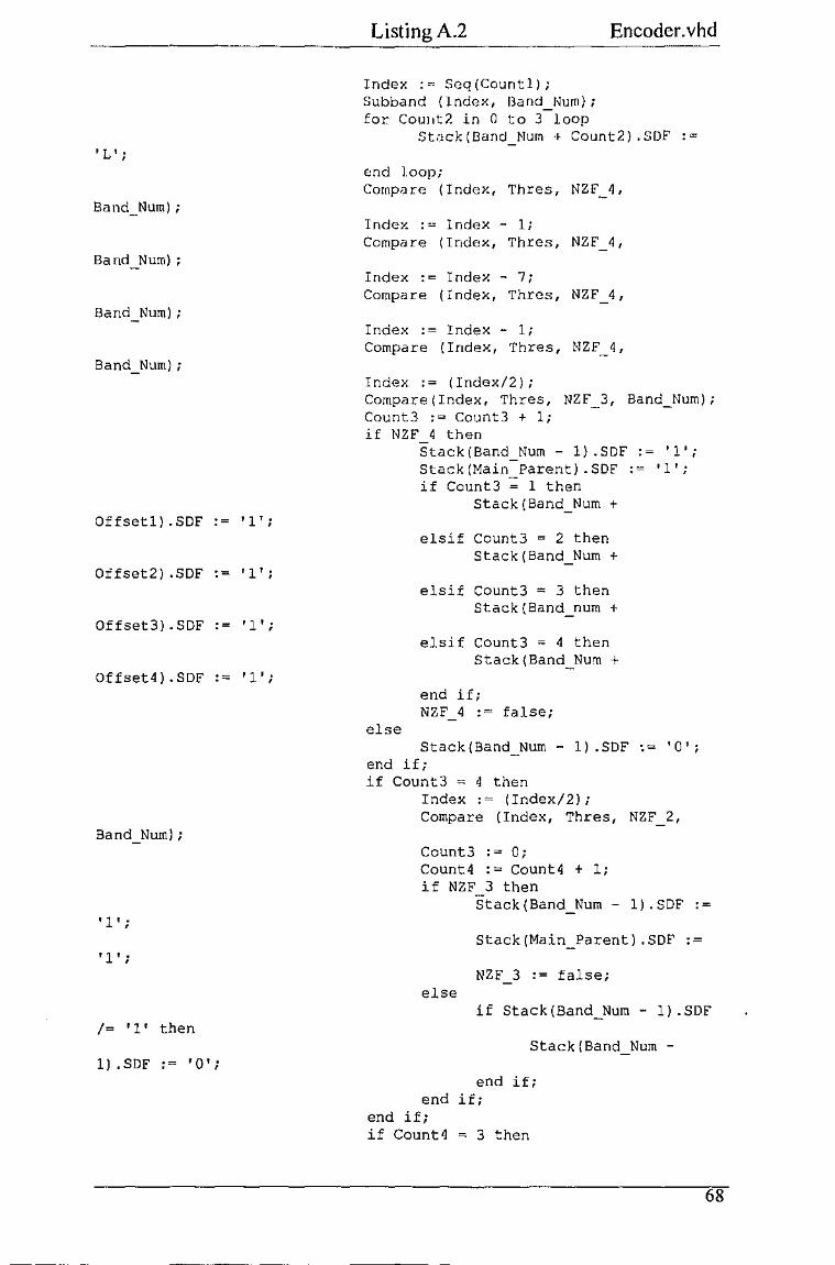
I L I;
Band_Num);
Band _Num) ;
Band _Num);
Band_Num};
Offsetl). SDF := '1' ;
Offset2) .SDF := r 1';
Offset3) .SDF := I 1 I j
Offset4). SDF !"' I 1' j
Band_Num);
• 1.;
• 1' ;
/= '1' then
1) .SDF ·= '0';
Listing A.2 Encoder.vhd
lndex :~ Scq(Countl); Subband (lndcx, 13and_Nurn); for Cou11t2 in 0 to 3 loop
St~ck{Band Num -~ Count2) .SDF :=
end loop; Compare (Index, Thres, NZF_4,
Index :~ lndex- 1; Compare (Index, Thres, NZF_4,
Index := Index - 7; Compare (Index, Thrcs, NZF_4,
Index := Index - 1; Compare (Index, Thres, NZF_4,
Index := (Index/2); Compare(Index, Thres, NZF_3, Band_Num); Count3 := Count3 + 1; if NZF 4 then
else
Stack(Band Num- 1) .SDF := '1'; Stack(Main_Parent) .SDF := '1'; if Count3 = 1 then
Stack(Band_Num +
elsif Count3 = 2 then Stack(Band_Num +
elsi£ Count3 = 3 then Stack(Band_num +
elsif Count3 ~ 4 then Stack{Band_Num +
end if; NZF 4 := false;
Stack{Band_Num - 1) .SDF ;= '0'; end if; if Count3 = 4 then
Index := {Index/2); Compare {Index, Thres, NZF_2,
Count3 := 0; Count4 := Count4 + 1; if NZF 3 then
Stack(Band_Num - 1) .SDF :=
Stack(Main_Parent) .SDF :=
NZF_3 := false; else
if Stack(Band_Num - 1) .SDF
Stack(Band_Num-
end if; end if;
end if; if Count4 = 3 ~hen
68
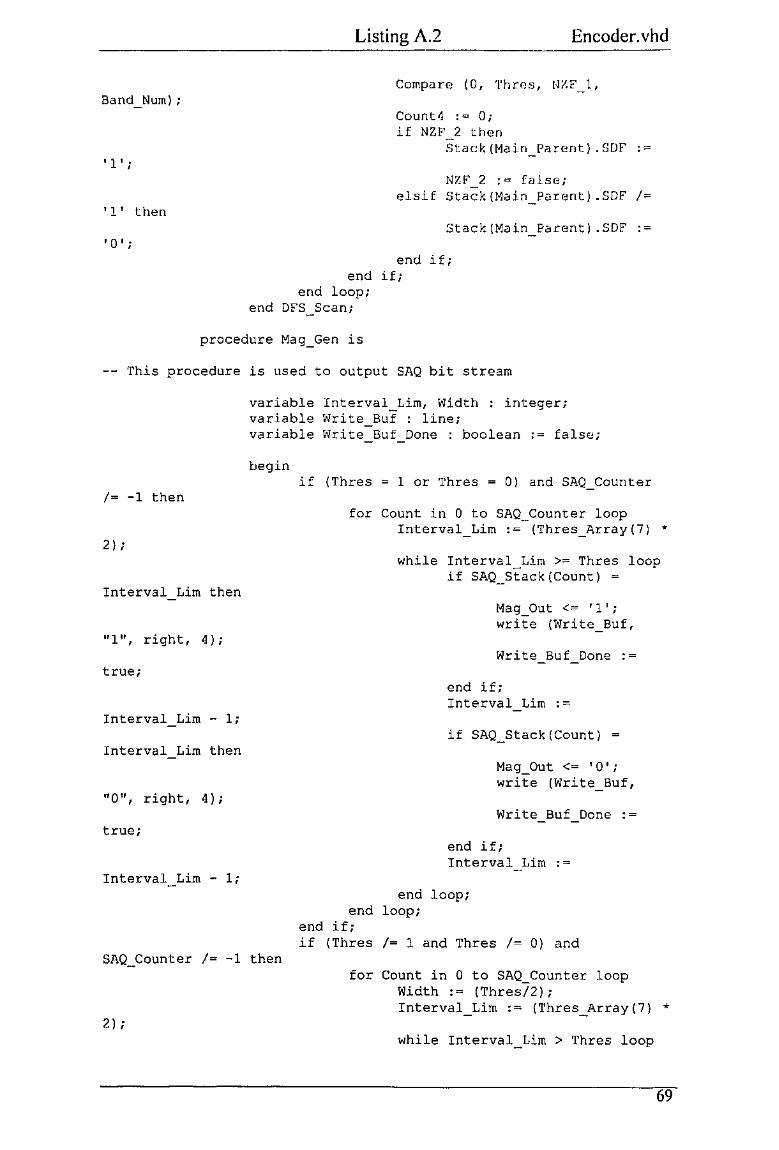
Band_Num);
' 1' i
'1' then
'0' ;
Listing A.2 Encoder. vhd
Compare (0, 'l'hrr)s, Nf,E'_l,
Count4 := 0; if NZI'' 2 then
Stack (Main Parent) . SDF :"'
NZF_2 :"' false; elsif Stack(Main Parent) .SDF /""
Stack(Main_Parent) .SDF :=
end if; end if;
end loop; end DFS_Scan;
procedure Mag_Gen is
-- This procedure is used to output SAQ bit stream
!~ -1 then
2) i
Interval Lim then
"1", right, 4 I ;
true;
Interval Lim - 1;
Interval Lim then
"Q" 1 right, 4) ;
true;
Interval Lim - 1;
variable Interval_Lim, Width : integer; variable Write_Buf : line; variable Write Buf Done : boolean := false;
begin if (Thres = 1 or Thres = 0) and SAQ_Counter
for Count in 0 to SAQ_Counter loop Interval_Lim := (Thres_Array(7) *
while Interval Lim >= Thres loop if SAQ_Stack(Count) =
Mag_ Out <~ '1'; write (Write_Buf,
Write Buf Done :=
end if; Interval Lim : =
if SAQ_Stack(Count)
Mag_ Out <= '0'; write (Write_Buf,
Write Buf Done :=
end if; Interval Lim : =
end loop; end loop;
end if; if (Thres /= 1 and Thres /= 0) and
SAQ_Counter /= -1 then
2) ;
for Count in 0 to SAQ_Counter loop Width := (Thres/2); Interval_Lim := (Thres_Array(7) *
while Interval Lim > Thres loop
69

Listing A.2 Encoder.vhd
j_f
(Interval_Lim>,SAQ_Stack(Count)) and (SAQ_f:itack(Counl)>lnter.val LirnWidth) then
"1", right, 4);
true;
t1ag_Out <= '1'; write (Write Buf,
!rlrite Buf Done :=
end if; Interval Lim :=
Interval Lim - Width; if
(Interval_Lim>,SAQ_Stack(Count)) and (SAQ_Stack{Count)>Interval LimWidth) then
"0", right, 4);
true;
Mag_Out <= '0'; write (\'1rite_Buf,
Write Buf Done :=
end if; Interval Lim :=
Interval Lim - Width; end loop;
end loop; end if; if Write Buf Done then
writeline (Mag File, Write_Buf); end if;
end Mag_ Gen;
procedure Sym_Gen is
-- This procedure is used to output SMAP symbols
(Stack(Caunt} .Sig
+ 1;
Stack(Count) .Amp;
right, 4);
If) ) ;
(Stack(Count) .Sig
+ 1;
variable Write_Buf : line; variable Write Buf Done : boolean := false;
begin for Count in Stack_Length downto 0 loop
if Stack(Count) .MSig /= '1' then
'1') then
'1') then
if (Stack(Count) .Sign= '0') and
Sym_Out <= Pas; Stack(Count) .MSig := '1'; SAQ_Counter := SAQ_Counter
SAQ_Stack(SAO_Counter) :=
write (Write_Buf, "Pas",
write (Write_Buf, string'("
Write_Buf Done := true; end if; if (Stack(Count) .Sign '1') and
Sym _Out <= Neg; Stack(Count).MSig := '1'; SAQ_Counter := SAQ_Counter
70

Encoder. vhd Listing A.2 ------·-----------'"'-----------
Stack(Count) .Amp;
righr., 4);
" ) ) i
write (Write Buf, "N0g'',
write (Write __ Buf, string'("
Wri.te Buf Done := true; end if; if (Stack(Count) .Sig = '0') and
(Stack(Count) ,SDE' = '0') then
right, 4);
" ) ) ;
(Stack(Count) .SDF '1') then
right, 4);
") ) ;
Sym_Out <= Z'I'R; write (Tflri'::e_Buf, "ZTR",
"1rite (~;riLe_Buf, string'("
Stack Stack
(Count) . Sig (Count) . SDF
:= '-'; ·- ,_,. . - '
Write Buf Done ·=true; end if; if (Stack(Count) .Siq = '0') and
Sym_Out <= IZ; write (i'lrite_Buf, " IZ",
write (Write_Buf, string'("
Stack Stack Write
end if;
(Count) .Sig (Count) . SDF Buf Done :=
•- I- I • .- ' := '- r; true;
if (Stack(Count).Sig= '0') and (Stack(Count) .SDF = 'L') then
right, 4);
" ) ) ;
begin
Sym_Out <= Z; write (Write_Buf, " Z" '
write (Write~Buf, string'("
Stack (Count) .Sig := '-'; Stack (Count) .SDF := '-'; Write Buf Done := true;
end if; end if;
end loop; if Write Buf Done then
writeline (S}m_File, Write_Buf); end if;
end Sym_Gen;
for Process Count in 0 to Image_Size loop Indices : = o; SAQ_Counter := -1; for Count in 0 to 7 loop
readline (In_File, Ln); DWT_Coeff (DWT, Stack, Ln, Indices);
end loop; for Index in 7 downto 0 loop
wait for 25ns; next when (Index = 0) ; Thres := Thres_Array(Index); DFS_Scan;
71

Listing A.2 .
Out Filter; Sym_Gen; Mag_Gen;
end loop; end loop; wait;
end process; end architecture behaviour;
Encoder.vhd
72

Listing A.3 Test enc.vhd
EZW Test bench ·for encoder Written by Hung Huynh Hierarchical level 3
library IEEE, std, support, work;
use IEEE.std_logic_1164.all, std.standard.all, std.textio.all, support.Type_Def.all, work.all;
entity Test_Encoder is end Test_Encoder;
architecture Stimulus of Test Encoder is component Encoder
port (elk : in std_logic; Sym_Out Mag_Out : out std_logic);
end component;
signal elk : std logic; signal Sym_Out : Code_Type; signal Mag_Out : std_logic; signal Clock_Cycle : natural :~ 0;
begin
out Code_Type;
DUT Encoder port map (elk, Sym_Out, Mag_Out); process is
end Stimulus;
begin loop
Clock Cycle <~ Clock_Cycle + 1; elk<= '1'; wait for 25ns; elk<= '0'; wait for 25ns;
end loop; wait;
end process;
72

Listing A.4 Decoder.vhd
EZW Decoder Written by Hung Huynh Hierarchical level 4
library IEEE, std, in it, support;
use IEEE.std_logic 1164.all, std. standard. all, std.textio.all, Decode_Init.all, support.Type Def.all;
entity Decoder is port (elk in std_logic; Sym_In
std_logic); end Decoder;
architecture behaviour of Decoder is
begin process is
in Cocte·_Type; Mag_In in
file Magnitude_File : text open read_mode is "mag.dat"; file Symbol_File : text open read_mode is "sym.dat"; file Reconst_File : text open write_mode is "result.dat";
variable Storage : Storage_Type; variable Scan Index : Scan Index_Type; variable SAQ_Count : integer; variable ZTR_Root : boolean := false;
procedure Gen Index (-Index : out integer; Feedback in integer) is
-- This procedure is used to make a jump for an appropriate symbol
begin for Count in Feedback to Stack_Length loop
Index := Count; exit when not (Scan_Index(Count) .Done);
end loop; end Gen_Index;
procedure Process_Symbol {Index integer; Ln : in line) is
in integer; Feedback
-- This procedure is used to process input symbols
constant Main Parent : integer ·~ 0; constant Offsetl integer .- 1; constant Offset2 : integer .- 8; constant Offset3 : integer ·~ 9; constant Last Child : integer ·~ 27;
variable Ch: string (0 to 4);
begin read (Ln, Ch); if .(Ch = " Pos ") or {Ch " Neg ") then
out
73

Listing A.4 · Decoder.vhd
if Ch = " Neg " then
Storage(Scan_Index(Index) .Index_No) .Sign :~ '1'; end if; if Scan_Index(Index) .Index_No Stack_Length
then Feedback : = Inde.x;·
else Feedback .- Index + 1;
end if; Scan_Index(Index) .Done :=true; Scan_Index(Index) .SAQ_Counter :~ SAQ_Count; SAQ_Count :~ SAQ_Count + 1;
end if; if (Ch = " IZ ") or (Ch = '' Z ") then
if Scan_Index(Index) .Index_No Stack_Length then
Feedback := Index; else
Feedback := Index + 1; end if;
end if; if Ch = " ZTR u· then
if (Scan_Index(Index) .Index No (Scan_Index(Index) .Index No~ Offset2) then
Offset1) or
then
Feedback :~ Index + 21; elsif Scan_Index(Index) .Index_No
Feedback := Index + 20; elsif (Scan_Index(Index) .Index No
Main Parent and SAQ_Count ~ 0) then ZTR_Root := true;
Offset3
elsif Scan_Index(Index) .Index_No Last Child then
Feedback := Index + 4; else
Feedback ·~ Index + 5; end if;
end if; end Process Symbol;
procedure Decode SMAP is
This procedure is used to decipher SMAP symbols
Ln);
variable Ln : line; variable Feedback : integer; variable Valid Index : integer;
begin if SAQ_Count <~ Stack_Length then
readline (Symbol File, Ln); Feedback :~ 0; for Count in 0 to (Ln'length/5)-1 loop
Gen_Index(Valid_Index, Feedback); Process Symbol{Valid_Index, Feedback,
end loop; end if;
end Decode_SMAP;
74
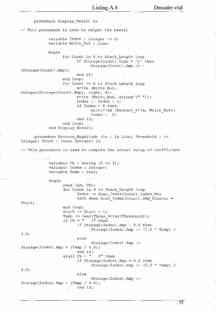
Listing A.4 Decoder.vhd
procedure DiSplay_Result is
This procedure is used to output the result
variable Index : integer := 0; variable Write Buf : line;
begin for Count in 0 to Stack_Length loop
if Storage(Count) .Sign~ '1' then Storage(Count) .Amp :~
(Storage(Count) .Amp); end if;
end loop; for Count in 0 to Stack Length loop
write (Write_Buf, integer(Storage(Count) .Amp), right, 4);
write {Write_Buf, string'("")); Index := Index + 1; if Index ~ 8 then
writeline (Reconst File, Write_Buf}; Index 0;
end if; end loop;
end Display_Result;
procedure Process Magnitude (Ln integer; Start : inout integer) is
in line; Threshold in
-- This procedure is used to compute the actual value of coefficient
Start;
4.0;
variable Ch: string (0 to 3); variable Index- : integer; variable Temp : real;
begin read (Ln, Ch); tor Count in 0 to Stack_Length loop
Index := Scan_Index{Count) .Index_No; exit when Scan_Index(Count) .SAQ Counter
end loop; Start := Start + 1; Temp:~ real(Thres_Array(Threshold)); if Ch = '' 1" then
if Storage(Index) .Amp~ 0.0 then Storage(Index) .Amp :~ (7.0 *Temp) I
else Storage(Index) .Amp :~
Storage(Index) .Amp+ (Temp I 4.0);
4.0;
end if; elsif Ch = " 0'' then
if Storage(Index) .Amp~ 0.0 then Storage(Index) .Amp :~ (5.0 *Temp) I
else Storage(Index) .Amp .
Storage(Index) .Amp- (Temp I 4.0); end if;
75

Listing A.4 Decoder.vhd
end if; end Process_Magnitude;
procedure Decode SAQ (Thres : in integer) is
This procedure is used to decipher SAQ bit stream
variable Ln : line; variable Start : integer;
begin if not ZTR Root then
readline (Magnitude File, Ln); Start :~ 0; for Count in 0 to (Ln'length/4)-1 loop
Process_Magnitude(Ln, Thres, Start); end loop;
end if; end Decode SAQ;
begin for Coeff Count in 0 to Image_Size loop
wait for 25ns; SAQ_Count :~ 0; Setup (Storage, Scan_Index); for Index in 7 downto 0 loop
next when (Index= 0); Decode SMAP; Decode SAQ (Index); ZTR Root :~ false;
end loop; Display_ Result;
end loop; wait;
end process; end architecture behaviour;
76

Listing A.5 Test dec.vhd
EZW test bench ·tor decoder Written by Hung Huynh Hierarchical level 5
library IEEE, std, support, work;
use IEEE.std_logic_1164.all, std.textio.all, support.Type Def.all, work.all;
entity Test Decoder is end Test Decoder;
architecture Stimulus of Test Decoder is component Decoder
port (elk : in std logic; Sym_In in Code_Type; Mag_In: in std_logic);
end component;
signal elk : std_logic; signal Sym_In : Code_Type; signal Mag~In : std_logic; signal Clock_Cycle : natural 0;
begin OUT Decoder port map (elk, Sym_In, Mag In);
process is begin
loop Clock_Cycle <~ Clock_Cycle
+ 1;
end Stimulus;
elk <= '1'; wait for 25ns; elk<= '0'; wait for 25ns;
end loop; wait;
end process;
77
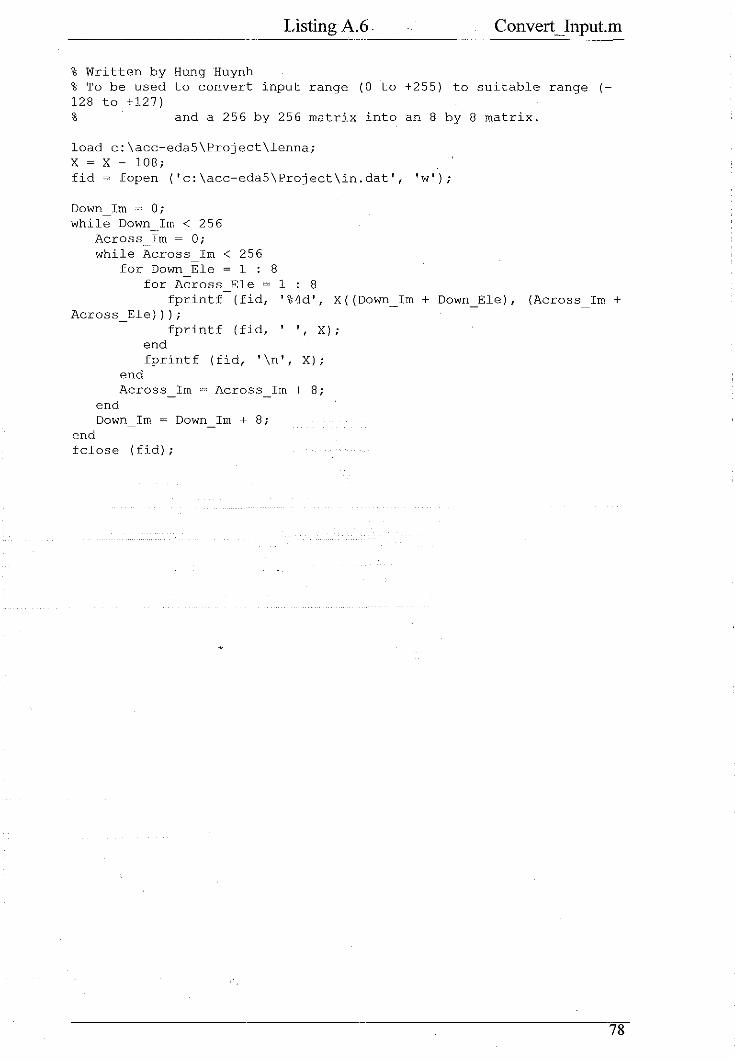
Listing A.6. Convert_Input.m
% Written by Hung Huynh % To be used to convert input range (0 to +255) to suitable range (-128 to +127) % and a 256 by 256 matrix into an 8 by 8 matrix.
load c:\acc-eda5\Project\lenna; X ~ X - 108; fid = fopen { 'c: \acc-edaS \Project \in. dat', 'w') ;
Down Im = 0; while Down Im < 256
Across _Im = 0; while Across Im < 256
for Down Ele ~ 1 : 8 for Across Ele = 1 : 8
fprintf (fid, '%4d', X((Down_Im + Down_Ele), {Across Im + Across_Ele)));
fprintf (fid, ' ', X); end fprintf (fid, '\n', X);
end Across Im =Across Im + 8;
end Down Irn = Down Im + 8;
end fclose I fid) ;
78

Listing A.7 Convert_ Output.m
% Written by Hung Huynh % To be used to convert input range (-128 to +127) to suitable range (0 to +255) % and an 8 by 8 matrix into a 256 by 256 matrix
load c: \acc-edaS \proj ect\result. dat; % load irnag.e into variable: result
x = zeros(256,256); %resulting matrix
for i ~ 1:32 %Read 32 blocks 8x8 to form one "row" 8x256 in result for j ~ 1:32
x( (i-1) *8+l:i*8, (j-1)*8+l:j*8) ~result( (i-1)*32*8+(jl) *8+1: (i-1) *32*8+j*8,:);
end end X = X + 108; imagesc (x); colormap gray;
load c:\lenna; err = X - x; mse ~ (norm (err, 'fro')A2)/(256*256); disp (' ')·; disp (' Distortion Measure in dB'); psnr ~ 10*logl0(255A2/mse); fprintf ('%6.2f\n', psnr)
79

Listing B.l Original Image of Lerma
50
100
150
200
250
50 100 150 200 250
Original Image of Lenna
80
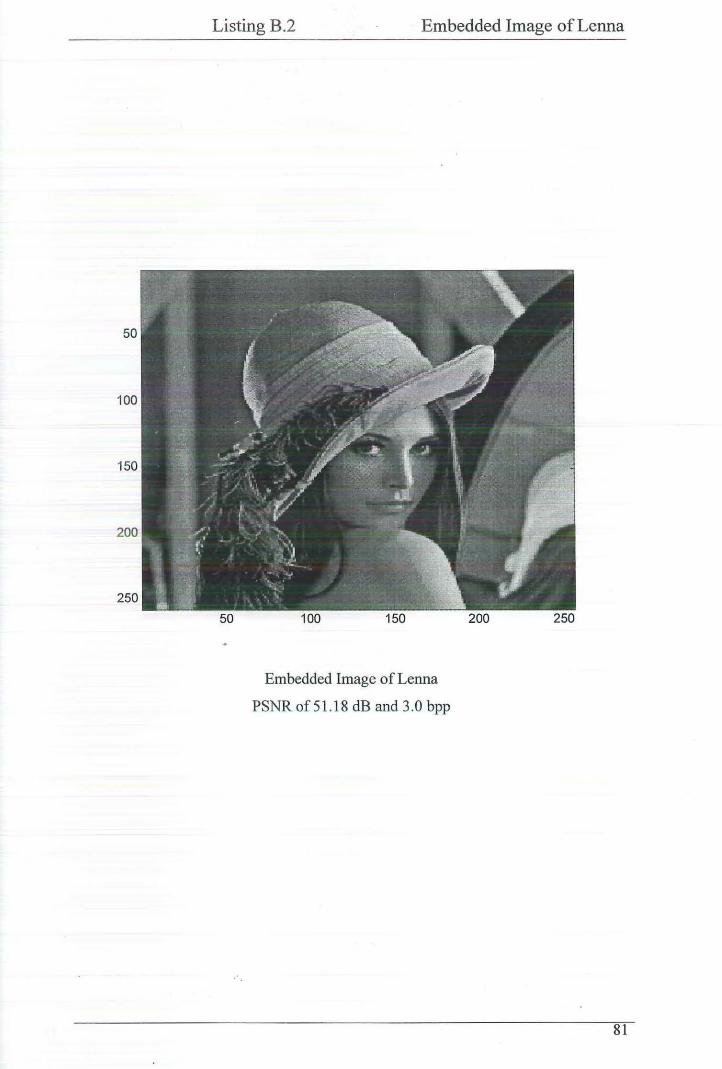
50
100
150
200
250
Listing B.2 Embedded Image of Lerma
50 100 150
Embedded Image of Lerma
PSNR of 51.18 dB and 3.0 bpp
200 250
81
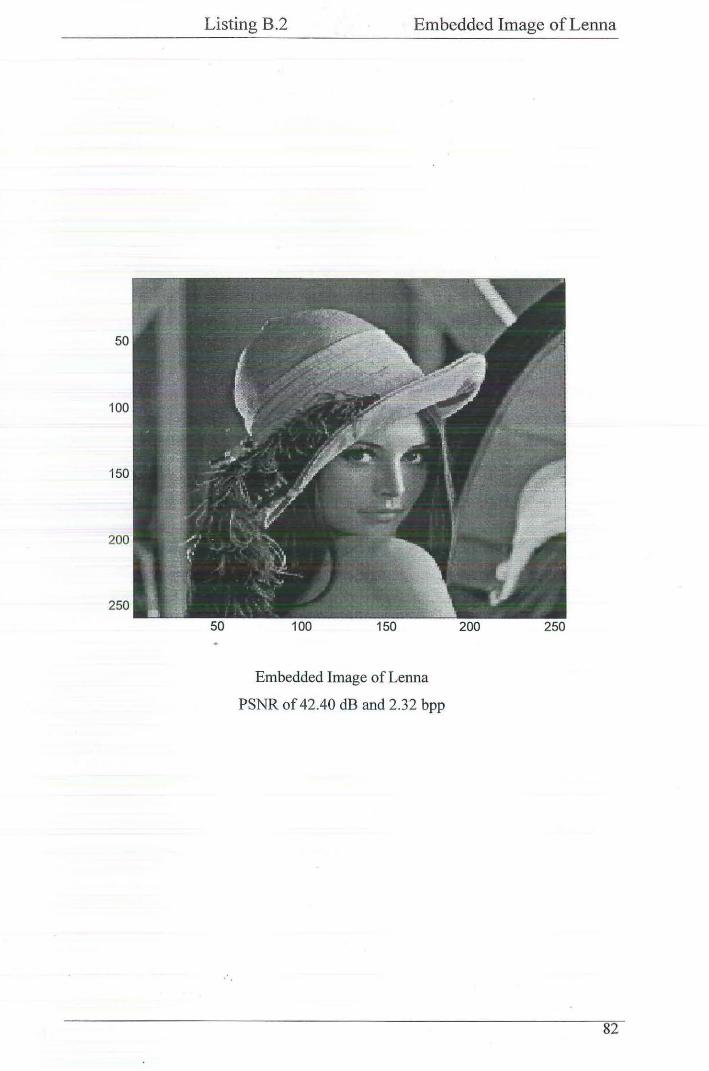
50
100
150
200
250
Listing B.2 Embedded Image of Lerma
50
..
100 150
Embedded Image of Lerma
PSNR of 42.40 dB and 2.32 bpp
200 250
82
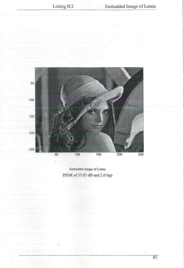
50
100
150
200
250
Listing B.2 Embedded Image of Lerma
50 100 150
Embedded Image of Lerma
PSNR of35.03 dB and 2.0 bpp
200 250
83

50
Listing B.2 Embedded Image ofLenna
..
Embedded Image of Lenna
PSNR of26.61 dB and 1.58 bpp
200 250
84
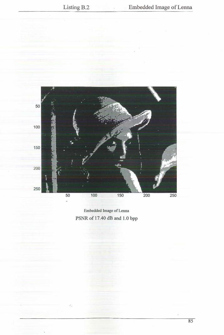
50
100
150
200
250
Listing B.2 Embedded Image of Lerma
50 100 150
Embedded Image ofLenna
PSNR of 17.40 dB and 1.0 bpp
200 250
85

1 1 1 1
1 0 0
. " 1 1
0 1 1
0 0 1
0 0 1
1 1 1
0 1 0
0 0 0
1 0 0
1 1 0
1 1 0
1 1 1
0 0 0
1 1 1 1
1 0 0 1
0 1 1 0
1 0 1 1
1 0 1 0
1
1
0 1 0
1 1 1
0 0 0 0
1 1 0 1
0 1 1 1
0 0 1 1
0 0 1 1
0 0
1 1 1
0 1 1 1
1
1
1 1
1 0 0
0
1 0
0 1 1
0 0 1 1
0
1
0 1 1
1 1 1
1 0 0 0
0 1 1 0
0 0 0 0
1 1 0 0
1 1 0 0
0 0
1 1 1
0 1 1 1
1 1 1 1
1
0
1
0
0 1 0
1 0 1
0 1
' 0 0 0
0 0 0 0
1 1 1 1
0 0 0 0
0 0 0 0
1 1 1 1
1 0 1 0
1 0 1 0
0 0
1 1 1
0 1 1 1
1
1 I
I 0 0 0
I I
I 0
I
1
0 0 I
I 1 0
1 1 0
1 1 1 1
0 0 0 0
0 0 1 0
1 0 1 1
0
0
1 0 1
1 0 1
0 0
1 1 1
0 1 1 1
Listing C. I
0
0
0
I
I
I
0
0 0 0
1 0
I 1 0
1 1 0
1 1
1 0
0 1 0
1 1 0 0
0 0 0 1
0 0 0 1
0 0 0 1
0 0
1 1 1
0 0 0 1
1
1 1 1 1
I [J
I
0
0 0
1
1
1 0 0
1 0 1
1 0 1
1 1 1 1
0 0 0 0
0 1 0 1
1 0 1 0
0 0 0 1
0 0 0 1
0 0
1 1 1
0 0 0 1
1 1 I 1
1 0 0 0
1 1 1
[I
0 0 Q
0 0 l 1
0
1
0 1 1
1 1 1
0 0 0 0
1 1 0 0
0 1 1 1
0 0 1 1
0 0 1 1
0 0
1 1 1
0 1 1 1
1 1
1
0 0 0
I 0 0
1 1
0
u (J
1 [J
0 1 l l
(j 0 ri 0
0 0 1 1
0 0 0 0 0 0 1 1
1 l 1 1 1 1 1 1
0 0 1 0 1 0 0 0
0 1 0 1 0 0 0 1
1 1 0 0 0 1 1 0
1 0 0 1 1 1 0 0
1 0 0 1 1 1 0 0
0 0 0 0
1 1 1 1 1 1
0 0 1 1 0 1 1 1
1
1 1
0 1 0
u 0
,,
0
0
0 Q
1 0 1
1 0 1
1 1 1 1
0 0 0 0
1 0 1 1
0 1 0 1
1 0 1 0
1 0 1 0
0 0
1 1 1
0 1 0 1
Typical Magnitude Output
0 1 1 () 0
0 l fJ
I
0 0 0 0 1 1
0 0 0 0 0 0
0 u 0 0 0 0
1 1 1 1 1 1
0 0 1 0 0 0
1 1 0 1 0 0
1 0 0 0 0 0
0 1 1 0 1 1
0 1 1 0 1 1
0 0 0 0
1 1 1 1
0 0 0 0 1 1
I I I
0 0
0 I I
1
0
0
1
1 1
1 1
1 1
1 1
0 0 0
0 1 0
1 1 1
1
1
1 1
1 1
0 0
1 1
0 0 1
l
1
1 1 1
0 1
1
(j
0
1 r;
1 0
1 1
0 0 0
0 1 0
1
0
1 1
0 1
0 0 1
0 0
1 1
0 0 0
r;
1
0
1
,, 'J
1
'J (j
0 0
1 1
0 0
1 0
0 0 1
0 1 0
0 1 0
0 0
1 1
0 0 0
,, ,,
'J f) I)
I '•
., .. ,,
0 G
! 'J
l 1 1 1 1 1
0 0 0 0 0 0
0 0 0 1 1 1
1 1 1 1 0 0
1 1 0 0 1 1
1 1 0 0 1 1
1 1 1 1 1 1
0 0 0 0 1 1
87
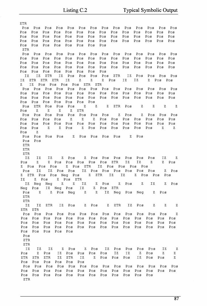
Listing C.2 Typical Symbolic Output
ZTR
Pas Pas Pas Pas Pas Pas Pas Pas Pas Pas Pas Pas Pas Pas
Pas Pas Pas Pas Pas Pas Pas Pas Pas Pas Pas Pas Pas Pas
Pas Pas Pas Pas Pas Pas Pas Pas Pas Pas Pas Pas Pas Pas
Pas Pas Pas Pas Pas Pas Pas Pas Pas Pas Pas Pas Pas Pas
Pas Pas Pas Pas Pas Pas Pas Pas
ZTR
Pas Pas Pas Pas Pas Pas Pas Pas Pas Pas Pas Pas Pas Pas
Pas Pas Pas Pas Pas Pas Pas Pas Pas Pas Pas Pas Pas Pas
Pas Pas Pas Pas Pas Pas Pas Pas Pas Pas Pas Pas Pas Pas
Pas Pas Pas Pas Pas Pas Pas Pas Pas Pas Pas Pas Pas Pas
Pas
IZ
IZ
Pas
IZ
ZTR
Pas
ZTR
ZTR
Pas
IZ
ZTR
Pas
Pas
IZ
Pas
Pas
z
Pas
Pas
z
Pas
Pas
z
ZTR
Pas IZ
IZ Pas
IZ
Pas
z
Pas
Pas
Pas
Pas
Z IZ Pas Pas Pas Pas ZTR ZTR
Pas
Pas
Pas
Pas
Pas
Pas
Pas
Pas
Pas
Pas
ZTR
z
Pas
Pas
Pas
Pas
Pas
z
Pas
Pas
Pas
Pas
Pas
z
Pas
Pas
Pas
Pas
Pas
z
Pas Pas Pas Pas Pas
Pas Pas Pas Pas Z
Pas
Pas
Pas
Pas
Pas
z
Pas
z
Pas Pas
Z Pas
Pas
Pas
Pas
Pas
z
ZTR
Pas
z
Pas
z
Pas
Pas
Pas
Pas
z
Pas
Pas
Pas
z
Pas
Pas
Pas
ZTR
Pas
Pas
Pas
Pas
Pas
Pas
Pas
z
Pas
Pas
Pas
z
Pas
Pas
Pas
z
Pas
Pas
Pas
z
Pas Pas Z Pas Z Pas Pas Pas
Z Pas Pas Pas Pas Pas Pas Pas
Pas
Pas
Pas
Pas
Pas
Pas
Pas
Pas
Pas
Pas
Pas
Pas
Pas
z
Pas
z
Pas Pas Pas Pas
Pas Pas
Z Pas Pas Pas Pas Z Pas
ZTR
ZTR
ZTR
IZ IZ IZ z Pas
z z Pas
z Pas Pas Pas
ZTR
Pas
IZ
Pas
IZ
Pas
z
IZ Z
Z Pas Pas
z Pas Pas
IZ
Pas
Pas
Pas
z
Pas Pas
Pas ZTR
Pas
IZ Pas Pas Pas Pas
Pas
Z ZTR
IZ
IZ
IZ Pas Pas
Pas Neg Pas
Z Pas ZTR
z z
IZ
z
IZ
Pas Pas
ZTR IZ
z
Pas Pas
IZ
z Pas
Pas
Z Pas
z
Neg
Pas
ZTR
ZTR
Z Pas
Neg Neg
Pas IZ
z
Neg
Pas
Pas
Neg
IZ z
Pas
Pas
IZ
ZTR
Neg z
IZ IZ ZTR
ZTR ZTR
IZ Pas
z z
Z Pas Z ZTR
Pas Neg
IZ Pas
Pas
Pas
IZ
z
z
Z Pas
Pas
Z Pas
Pas
z z
Pas Pas Pas Pas Pas Pas Pas Pas Pas Pas Pas Pas Pas Z
Pas Pas Pas Pas Pas Pas Pas Pas Pas Pas Pas Pas Pas Pas
Pas Pas Pas Pas Pas Pas Pas Pas Pas Pas Pas Pas Pas Pas
Pas Pas Pas Pas Pas Pas Pas Pas Pas Pas Pas Pas Pas Pas
Pas Pas Pas Pas Pas
Pas
ZTR
ZTR
IZ
Pas
ZTR
IZ
z
ZTR
IZ
Pas
ZTR
IZ
IZ
z Pas
Pas
ZTR
Pas
IZ
Pas Pas Pas Pas Pas Pas
z Pas
Pas
z
IZ
Pas
Pas
Pas
IZ
Pas
Pas
IZ
Pas
Pas
z
IZ
Pas
Pas
Pas
IZ
z
Pas
z
z
z
Pas Pas Pas Pas Pas Pas Pas Pas Pas Pas Pas Pas Pas Pas
Pas Pas Pas Pas Pas Pas Pas Pas Pas Pas Pas Pas Pas Pas
Pas Pas Pas Pas Pas Pas Pas Pas Pas Pas Pas Pas
ZTR
87