1

Universidad de Chile

Facultad de Economía y Negocios

Escuela de Economía y Administración

Vessel Routing Problem Under Uncertainty of

Demand

Seminario para optar al título de

Ingeniero Comercial, Mención Administración

Participantes

Felipe Andrés Vega Fink

Profesor Guía

Juan Pablo Torres Cepeda

Santiago de Chile – 10 de diciembre de 2014

2

Contents

Abstract ........................................................................................................................................... 3

1. Introduction ................................................................................................................................ 3

2. Literature Review ...................................................................................................................... 5

3. Problem Description .................................................................................................................. 7

4. Formulation of the Problem ....................................................................................................... 9

4.1 VRP formulation ....................................................................................................................... 9

4.2 Demand Uncertainty ............................................................................................................... 12

4.3 Income-Cost equilibrium ........................................................................................................ 14

5 Experimental analyses ............................................................................................................... 16

6 Conclusions ................................................................................................................................ 17

References ..................................................................................................................................... 18

Tables

Table 1 Respective distributions assigned to fit each port. ........................................................... 13

Table 2 Result of NB scenarios .................................................................................................... 17

Table 3 Results of SB scenarios.................................................................................................... 17

Equations

VRP Formulations ( 1 )-( 10 ) ....................................................................................................... 11

VRP Formulations ( 11 )-( 19 ) ..................................................................................................... 12

Demand Uncertainty ( 20 )-( 23 ) ................................................................................................. 14

Demand Uncertainty ( 24 )-( 30 ) ................................................................................................. 15

Income-Cost Equilibrium ( 31 )-( 35 ) .......................................................................................... 16

3

Vessel Routing Problem Under Uncertainty of

Demand

Abstract In this paper it is introduced an optimization to solve the Vehicle Routing Problem (VRP) with

uncertainty of demand. The focus is to minimize the transportation costs while satisfying all the

given constraints of the problem. The demand uncertainty is solved by applying a distribution

fitting to the historical demand data provided by a break-bulk sea shipping company; therefore

this is a real world implementation of the VRP with uncertainty of demand. Various scenarios

are generated, each with randomized demand from each port’s distribution.

Keywords: Optimization, vehicle routing, demand uncertainty, distribution fitting

1. Introduction

Many transport optimization models have been developed to improve the performance in the

shipping industry. Several models focus on reducing cost and transit time, for land, air or sea

transportation (Okita et al. 2004).

Sea shipping has been standardized to optimize performance, where the biggest breakthrough

was the introduction of the container. These reusable steel boxes provided easier transportation,

optimizing space, standardizing gear for the load and discharge process and even to protect the

goods in a safer way. Since the beginning of the containerization in early 1960s to 1990, the

trade grew from 0.45 trillion dollars to 3.4 trillion dollars. It grew by a factor of 7. (Bernhofen et

al., 2013)

However, not every cargo fits in a container, projects like a windmill, an oversized gear, or

heavy machinery. Also there is cargo that is inefficient to consolidate in a container like metal,

cement, concentrate, or grain (Bornozis, 2006). And other cargo preferred to avoid containeriza-

tion because of their size. Most break bulk cargoes are highly valuable products. (Shipping Aus-

tralia’s Break Bulk Shipping Study). Break-Bulk carrier is a ship that has wide vaults to carry

cargo, which can carry volumetric cargo that would not fit in a container.

4

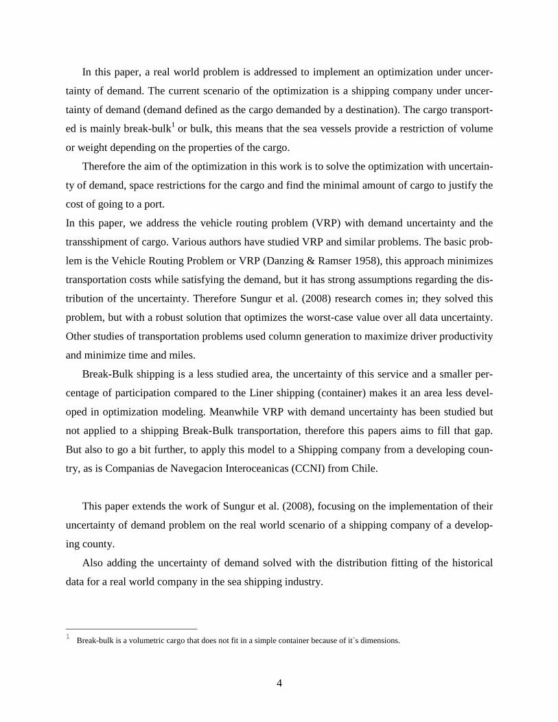
In this paper, a real world problem is addressed to implement an optimization under uncer-

tainty of demand. The current scenario of the optimization is a shipping company under uncer-

tainty of demand (demand defined as the cargo demanded by a destination). The cargo transport-

ed is mainly break-bulk1 or bulk, this means that the sea vessels provide a restriction of volume

or weight depending on the properties of the cargo.

Therefore the aim of the optimization in this work is to solve the optimization with uncertain-

ty of demand, space restrictions for the cargo and find the minimal amount of cargo to justify the

cost of going to a port.

In this paper, we address the vehicle routing problem (VRP) with demand uncertainty and the

transshipment of cargo. Various authors have studied VRP and similar problems. The basic prob-

lem is the Vehicle Routing Problem or VRP (Danzing & Ramser 1958), this approach minimizes

transportation costs while satisfying the demand, but it has strong assumptions regarding the dis-

tribution of the uncertainty. Therefore Sungur et al. (2008) research comes in; they solved this

problem, but with a robust solution that optimizes the worst-case value over all data uncertainty.

Other studies of transportation problems used column generation to maximize driver productivity

and minimize time and miles.

Break-Bulk shipping is a less studied area, the uncertainty of this service and a smaller per-

centage of participation compared to the Liner shipping (container) makes it an area less devel-

oped in optimization modeling. Meanwhile VRP with demand uncertainty has been studied but

not applied to a shipping Break-Bulk transportation, therefore this papers aims to fill that gap.

But also to go a bit further, to apply this model to a Shipping company from a developing coun-

try, as is Companias de Navegacion Interoceanicas (CCNI) from Chile.

This paper extends the work of Sungur et al. (2008), focusing on the implementation of their

uncertainty of demand problem on the real world scenario of a shipping company of a develop-

ing county.

Also adding the uncertainty of demand solved with the distribution fitting of the historical

data for a real world company in the sea shipping industry.

1 Break-bulk is a volumetric cargo that does not fit in a simple container because of it`s dimensions.

5

The structure of this paper is organized as follows. Section 2 presents the relevant literature

for this case. The problem is presented in Section 3, which shows the characteristics of the situa-

tion to optimize the model. Section 4 presents formulations of the vessel routing problem de-

mand uncertainty. Experimental results are shown and analyzed in Section 5. And the paper

concludes in section 6 with a discussion of the main findings and conclusions.

2. Literature Review

A wide range of literature concerning vehicle routing optimization and intermodal freight

transportation is currently available. Escudero et al. (2012) solved the drayage problem with

transit time uncertainty. They applied two different methods, the first was a Two-Phase heuristic

algorithm, where all possible combinations of tasks are analyzed and then combined tasks are

inserted into routes. And the second methods was a Genetic Algorithm, which is a stochastic

metaheurisic algorithm based on the evolutionary theory. To improve performance they intro-

duced the concepts of penalty costs of certain actions and improvement factor, which demands a

certain minimum of improvement to change the current combination. The comparison of the two

possible methods ended with the first one as the best fitted for the task, because of the speed to

solve and the flexibility of adaption. Katayama & Yurimoto (7th

International Symposium on

Logistics) focused on the Load Planning Problem for Less-than-Truckload. The method to solve

the problem was a Lagrangian Relaxation (LR), the results of the experimentation suggested that

the (LR) can perform a good job of identifying a lower bound of the problem, but it is lacking an

adaptation to the real world. Ileri et al. (2006) focused on minimizing the cost of daily drayage

operations. The column-generation with Tree Orders was used to solve the problem and to find

cost-effective schedules. Sun et al. (2014) extends and refines the work done in Ileri et al. (2006).

The focus was on fast solving an optimization of daily dray operations across intermodal freight

network in the face of constant changing data. This problem focused on maximizing driver’s

productivity meanwhile minimizing miles and time. And continue with the column-generation

considering traffic congestion, integration with commercial transportation system and address

imbalance of empty containers that get accumulated in certain regions.

In Arnold et al. (2003) was modeled an intermodal transportation system. The model fo-

cused on optimally locating rail or road terminals for freight transport. To solve the model a heu-

6

ristic approach was used. The paper aims to analyze the impact of variations in the supply of

transport of the rail and road freight transport in the Iberian Peninsula. The heuristic method was

used due to the requirement of time limit to provide a solution.

Powell & Koskosidis (1992) applies a tree constraint to solve a shipment routing sub

problem that is extracted from real world considerations. A family of algorithms is investigated

to find a solution to the routing sub problem. The used algorithms are a Hierarchical solution,

Gradient-Based local search and Primal Dual Methods. The Primal Dual Methods analyzed

where the Sub gradient Optimization (SGO), Multiplier Adjustment Algorithm and Dual Ascent

Algorithm. The SGO algorithm showed the best execution time and quality of the upper and

lower bounds. Therefore the SGO is the best suited seems best suited to provide a good solution

in relatively short time.

Varelas et al. (2013) is a paper that presents a toolkit that Danaos Corporation developed

to optimize ship routing. The toolkit, named ORISMAS, solves the problem of least-cost voyage

versus faster voyage. This is achieved through the integration of financial data, hydrodynamic

models, weather conditions, and marketing forecasts. Due to ORISMAS in 2011 the revenues

where increased in $1.3 million from time saving and $3.2 million from fuel savings. This is

considering 30 vessels that where operated with ORISMAS.

Christiansen et al. (2003) made a literature review of the current status of ship routing

and scheduling up to the year 2003. Christiansen et al. (2003) provides relevant research to in

terms of liner and tramp. Liner services are defined as a bus line, because it operates with a pub-

lished itinerary that the ship must stick to it. The Liner shipping must take decisions at different

instances, such as route and schedule design, fleet size and mix (combinations of cargoes to max-

imize revenues), fleet deployment and cargo booking (choose which cargoes are accepted or re-

jected for the voyages).

A tramp services follows the available cargoes, it works like a taxi. Compared with in-

dustrial shipping (such as oil) this area has been less researched. Principally this is due to the

large number of small operations in the tramp business. Tramp ships follow the available cargo

to transport and sometimes they reach agreements that specify quantities, destinations, transit

time and a payment per ton. The optimization is done as maximization instead of industrial ship-

ping considering both costs and revenues. The optimization is done with a LP-Relaxed solution

approach with a sub problem of shortest path. Other was solved with formulated as a set packing

7

problem with an algorithm for generating all possible schedules a priori. Fagerholt (2003) devel-

oped a heuristic hybrid search algorithm to solve the ship scheduling problems. Also the paper

comments the differences of sea transport with other types. Ships pay port fees; draft is a func-

tion of weight of the load that affects the possibility to dock in ports. Plus the ports operate in

international trade, therefore crossing multiple jurisdictions. And the ships can be diverted at sea.

Dumas et al. (1990) takes a generalization of the Vehicle Routing Problem (VRP) that is

the pick up and delivery problem with time windows (PDPTW). The VRP focuses on providing

a design of routes that present minimum cost for a set of vehicles that service a known demand.

The PDPTW constructs an optimal route to satisfy different requests, such as pickup and deliver

under capacity, time windows and precedence constraints. The algorithm used is a column gen-

eration algorithm scheme with a constrained shortest path as sub problem. The findings are that

the time windows and the distribution of pickup demand are the most significant parameters,

both having higher influence on the running time of the algorithm. If the nodes in the problem

are fewer than ten, then the shortest path is an efficient way to generate feasible routes.

Sungur et al. (2008) addresses the problem of uncertainty of demand and considering

this, use the robust approach. The robust solution provides a good solution for all possible data

uncertainty. A normal VRP solution just will find an optimal value, which due to the uncertainty

could not be a good solution. The robust solution is an attractive option to formulate the problem,

since it does not require distribution assumptions on the uncertainty. This model will be adapted

in this work to solve the current problem of a break-bulk shipping company.

3. Problem Description

As the break-bulk transportation was relegated to a secondary concern, few models at-

tempted to develop models of optimization for this sort of transportation and fewer for a compa-

ny that is located in a developing country. As any transportation problem there is the trade off

between a least-cost voyage and a faster voyage (cost savings against time savings). The least-

cost voyage is affected by a variety of expenses. The Bunker cost (fuel cost) is one of the most

important in this industry; it is a key component for the whole sea shipping industry. The cost is

determined by the amount of bunker consumed in the route and by the price of the IFO140 and

MDO, which are determined by the trading markets. The company is a price taker on the fuel

market and does not considering derivatives to reduce the price variation. Every sea vessel has

8

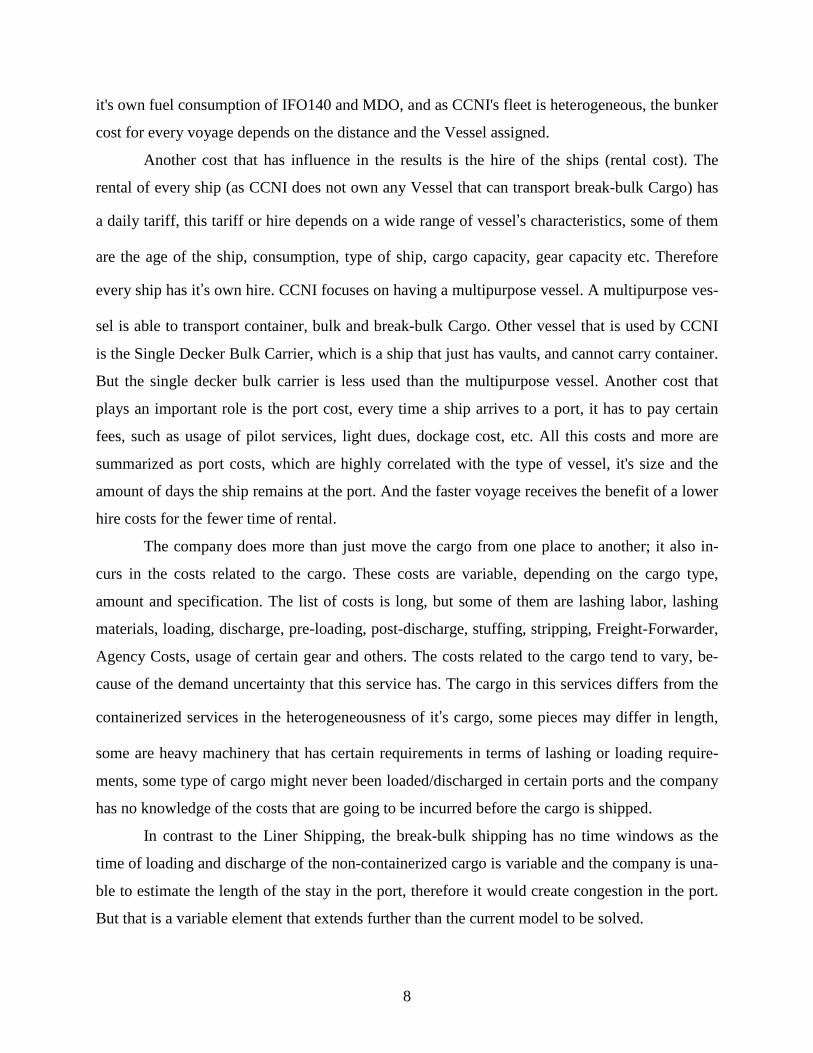
it's own fuel consumption of IFO140 and MDO, and as CCNI's fleet is heterogeneous, the bunker

cost for every voyage depends on the distance and the Vessel assigned.

Another cost that has influence in the results is the hire of the ships (rental cost). The

rental of every ship (as CCNI does not own any Vessel that can transport break-bulk Cargo) has

a daily tariff, this tariff or hire depends on a wide range of vessel’s characteristics, some of them

are the age of the ship, consumption, type of ship, cargo capacity, gear capacity etc. Therefore

every ship has it’s own hire. CCNI focuses on having a multipurpose vessel. A multipurpose ves-

sel is able to transport container, bulk and break-bulk Cargo. Other vessel that is used by CCNI

is the Single Decker Bulk Carrier, which is a ship that just has vaults, and cannot carry container.

But the single decker bulk carrier is less used than the multipurpose vessel. Another cost that

plays an important role is the port cost, every time a ship arrives to a port, it has to pay certain

fees, such as usage of pilot services, light dues, dockage cost, etc. All this costs and more are

summarized as port costs, which are highly correlated with the type of vessel, it's size and the

amount of days the ship remains at the port. And the faster voyage receives the benefit of a lower

hire costs for the fewer time of rental.

The company does more than just move the cargo from one place to another; it also in-

curs in the costs related to the cargo. These costs are variable, depending on the cargo type,

amount and specification. The list of costs is long, but some of them are lashing labor, lashing

materials, loading, discharge, pre-loading, post-discharge, stuffing, stripping, Freight-Forwarder,

Agency Costs, usage of certain gear and others. The costs related to the cargo tend to vary, be-

cause of the demand uncertainty that this service has. The cargo in this services differs from the

containerized services in the heterogeneousness of it’s cargo, some pieces may differ in length,

some are heavy machinery that has certain requirements in terms of lashing or loading require-

ments, some type of cargo might never been loaded/discharged in certain ports and the company

has no knowledge of the costs that are going to be incurred before the cargo is shipped.

In contrast to the Liner Shipping, the break-bulk shipping has no time windows as the

time of loading and discharge of the non-containerized cargo is variable and the company is una-

ble to estimate the length of the stay in the port, therefore it would create congestion in the port.

But that is a variable element that extends further than the current model to be solved.

9

The demand of break-bulk transportation is unstable and variable, due to fluctuations in produc-

tion, economic cycles, competitors, etc. Those are characteristics of the spot market as is the

break-bulk. Contracts are hard to get and the price competition generates a price war. For this

reason, the demand for the service has to be estimated to solve the optimization problem. An

analysis of distribution of the demands has to be done in order to archive an optimum solution.

The demand can be divided in North Bound (NB) and South Bound (SB).

4. Formulation of the Problem

4.1 VRP formulation

The formulation of the problem is the following:

The ship has a volume capacity of V cbm2, a weight capacity of W tons, and a container ca-

pacity of T Teu3, to consider the limitations of the vessels. Let P be the set of ports. Whether or

not a cargo is shipped from port i to j depends on and it takes value 1 if the cargo k is trans-

ported from to port i to port j. is the variable that represents the variable costs of the cargo k

that is originated from port “i” has as destination port “j”. is the volume of cargo k and is ex-

clusive to the cargo that goes SB. is the weight of the cargo k that only takes a value other

than cero if the cargo goes NB. Also refers to the amount of teus, is particular to the car-

goes k’s that are containerized.

is the variable that denotes the number of days that takes a voyage between ports i and j.

is a variable that determines the if the vessel sails from port i to port j. Takes value 1 if the

vessel sails from port i to port j and cero other case.

is the port cost of port i and is the variable that shows how many times the vessel is to

be docked at the port i, therefore can only take integer values.

B is the bunker price designated for the voyage and H is the hire (price per day) for the ves-

sel.

2 Cbm: cubic meter 3 TEU: Twenty-foot equivalent unit

10

is a binary variable that takes value 1 if cargo is to be shipped to port i. And is a binary

variable that takes value 1 if cargo is to be shipped from port i.

, and respectively denote the total volume, weight and teus of the cargoes when the

vessel sails from port i.

And , and, are the demands of port i for volumetric cargo, normal cargo (weight

cargo) and containerized cargo respectively.

( 1 )

( 2 )

( 3 )

( 4 )

( 5 )

( 6 )

( 7 )

( 8 )

11

( 9 )

( 10 )

( 11 )

( 12 )

( 13 )

( 14 )

for

( 15 )

for

( 16 )

( 17 )

( 18 )

12

( 19 )

The constraint ( 1 ) represents the objective function to minimize, with considering all the

costs related to the model. Constrain ( 2 ) restricts the vessel to be able to transport cargo just

one time. The constraint ( 5 ) imposes the ship to go to port i when cargoes that are going to be

transported have port i as origin or destination. Constraints ( 6 ) and ( 7 ) impose that the vessel

has to arrive to or sail from a certain port due to the supply of cargo. Constraints ( 8 ) - ( 13 ) are

the cargo flows from the ports. Constraints ( 14 )-( 16 ) are the vessel’s capacity restrictions. The

constraints ( 17 ) - ( 19 ) are demand limitations where cargo transported to port i cannot be

higher than it’s demand in terms of volume and weight.

4.2 Demand Uncertainty

The optimization mentioned in section 4.1 represents a problem where the demand is cer-

tain and the company has knowledge of the demand of cargoes. But for this services most of the

time, mainly earlier to the three weeks before the beginning of the voyage, demand is uncertain.

Therefore values , and are uncertain. To address that uncertainty an analysis of the

distribution of the historical values was made. The weekly distribution of each port was analyzed

and values where assigned, due to the considerable amount of observations that had cero cargo

transported, a double distribution was used. In the first stage a binominal distribution was used,

where 1 referred to a week when cargo is transported and cero otherwise. And this binominal

helped address the first part of the distribution of the demand. Later to combine the binominal,

the amount of cargo transported per week (volume, weight or teu) was fitted to distributions.

Each port has a specific distribution for the two demands, a demand of break-bulk cargo and

containerized cargo. This distribution assigns a random value of the total weekly demand for

each port. In Table 1 the first row show the different ports, each port has a break-bulk distribu-

tion for its demand that is the second column. And the containerized cargo distribution is shown

in the third column of the table. Also five new variables were added, the first pair are the random

13

binomial values for the demand of each port. refers to the break-bulk cargo and to the

containerized cargo. The other three variables are random numbers distributed fitted to the data

of the port and cargo type , and . The first is the random value of the total sum of

containers to be demanded by port i. and are the random values of the total break-

bulk cargo demanded by port i but separated by volume and weight.

Table 1 Respective distributions assigned to fit each port.

In consequence constraints ( 2 ) and ( 8 ) - ( 18 ) are no longer valid due to the lack of individual

cargo to be shipped. So a variation of that constraint is used. is replaced by and , those

are binomial variables for break-bulk and containerized cargo respectively. and , takes

value 1 if the total cargo from port i to port j is to be transported by the vessel. And , and

are reformulated to refer to the total volume, teus or tons that are demanded from port i to j.

( 20 )

Ports12

3

456

7

891011

12131415

BBDistrib TEUDistribINVGAUSS InvGaussLogNorm Expon

LogNorm -

InvGauss ExponInvGauss InvGaussInvGauss Expon

InvGauss -

Expon InvGaussPareto2 InvGaussWeibull InvGaussPert Weibull

Expon ExponTriang InvGaussPert Expon- Expon

14

( 21 )

( 22 )

( 23 )

( 24 )

( 25 )

( 26 )

( 27 )

( 28 )

( 29 )

15

( 30 )

With this reformulation of the problem in 3.1, the uncertainty of demand is solved and the prob-

lem can work with an estimated demand that is based on the distribution of the historical de-

mand. Now the problem can be solved even weeks in advance.

4.3 Income-Cost equilibrium

To improve the cost minimization, an analysis of the income and cost of the transported

cargo for each port was done. This has to be done due to the lack of information about cost asso-

ciated to the cargoes due to the fact that the demands of ports are uncertain. And to solve that,

random numbers with certain distribution were created, but no cost linked to those demands.

Therefore another tool has to be developed to consider the economically beneficial cargoes. The

income per amount of cargo was brought up against the cost per amount of cargo. As the econo-

mies of scale are present in this problem, the higher the amount of cargo, the bigger was the

growth of income in comparison to the growth of cost. Therefore equilibrium could be found to

set a minimum cargo that covers at least all the costs that the company will have to incur to

transport certain amount of cargo form a port.

( 31 )

( 32 )

( 33 )

( 34 )

16

and are the restrictions of container and break-bulk for port i, that were originated from

the income-cost equilibrium. The new variables and from constraints ( 31 ) and ( 32 ) take

value 1 if demand from port i is higher than the restriction. And constraints ( 33 ) and ( 34 ) re-

strict the cargo to be transported by the vessel to cero if the cargo demanded by port i is not supe-

rior to the restriction of port i. With the new properties of the estimated demand, the objective

function is reformulated extracting the costs related to cargoes. The new objective function is

( 35 )

5 Experimental analyses

In this section, the performance of the model is evaluated and parameters to apply a com-

parison will be determined. To measure the effectiveness of the model that has been created in

section 3, a set of scenarios were created. Each scenario has it’s own randomized demand for

each port, so each scenario is unique. The model will have to optimize every scenario in a differ-

ent way, therefore it will be possible to create a comparison of the different results and evaluate

the benefit of the model created. The results of the NB scenario are resumed in Table 2. The

table synthetizes the relevant information from the scenario after the optimization took place.

The first parameter is the sum of ports, which is the number of ports that the vessel will have to

visit in the respective scenario. The cost is the monetary value of the scenario. Demand CNT is

the demanded container cargo and the CNT transported represents the amount of TEU’s that are

transported considering the respective demand. Demand BB and BB Transported work in the

same logic as the previews columns but applied to the break-bulk cargo.

And the last column refers to the total distance that the vessel will have to sail that is

measured in nautical miles. The different scenarios provide a wide variety of information after

the constraints have been met. For instance in scenario 8 NB the break-bulk demand was 222.5

wt, but it does not exceed the equilibrium point stated for the ports, therefore none of the break-

bulk cargo should be loaded. Having a voyage with just 50 TEU’s to be shipped, turns out to be

17

unproductive. For this reason, the voyage in scenario 8 NB should be a blank sailing (no voyage

is made). Other important aspect is the automatic reduction of ports, if the cargo is not sufficient

to satisfy the port equilibrium constraints, then the port is skipped. As is the case of scenario 1

NB, where 5 ports are in the vessel’s itinerary in comparison with the 6 of scenario 2 NB or the 4

ports of scenario 4 NB. The omission of a port provides a variety of benefits such as the avoid-

ance of the port cost. Also bunker cost and hire cost due to the deviation in time and fuel con-

sumption.

Table 3 shows the same parameters Table 2 but applied to the scenarios of the SB voyag-

es. The results can be used and analyzed as in Table 2. For instance, the scenario 4 NB has the

lowest cost of the bunch of scenarios. But also has the lower amount of ports in the itinerary.

That can compensate the fewer cargo, therefore lower income that it will receive in comparison

to the like of scenario 6 where the cargo is almost the double with 3276.9 cbm.

Table 2 Result of NB scenarios

Table 3 Results of SB scenarios

ScenarioNB SumofPorts Costs DemandCNT CNTTransported DemandBB BBTransported Distance

1 5 $494.276 5 0 2377,9 2106,9 7221

2 6 $574.393 84 72 1114,7 1114,7 8334

3 6 $561.443 50 48 5975,1 5975,1 8080

4 4 $534.620 36 32 36,8 0 7779

5 6 $561.443 133 130 1651,2 1554,9 8080

6 6 $561.443 83 58 3732,8 3635,5 8080

7 5 $494.276 64 55 375,8 260,3 7221

8 5 $494.276 64 50 222,5 0,0 7221

9 5 $537.312 0 0 868,2 868,2 7814

10 6 $561.443 146 143 0 0 8080

ScenarioSB SumofPorts Costs DemandCNT CNTTransported DemandBB BBTransported Distance

1 8 $647.686 129 120 928 928 8910

2 8 $587.481 211 196 1319 1319 8004

3 7 $656.020 109 94 2038 2038 9388

4 6 $541.704 35 19 1972 1674 7916

5 8 $623.357 38 36 2452 2452 8828

6 8 $635.346 124 117 3277 3277 8942

7 9 $659.337 240 239 1900 1868 8929

8 6 $624.432 183 162 0 0 9057

9 6 $541.704 77 41 3642 3642 7916

10 9 $659.337 278 279 2545 2545 8929

18

6 Conclusions

In this study, a problem of a vehicle routing problem with uncertainty of demand was

proposed. This work has shown that it is feasible to implement a VRP with the distribution of

historical demand to solve the uncertainty in a real world scenario. The simple VRP was derived

to a transshipment problem, with constraints of capacity for volume, weight and quantity of con-

tainers. Also was implemented an equilibrium point of income versus cost, to provide the mini-

mum amount of cargo that brings a positive result to the operation. The work is applicable to a

real-world scenario that can provide relevant information such as when to implement a blank

sailing, which ports to omit despite that it has a demand of products, or even to end the voyage in

a port earlier than it should. With the measures the deficiency created by the lack of cargo can be

reduced. This study proofs that the VRP with the distribution of demand and equilibrium point is

feasible in the real world scenario. Moreover it can be applied to the sea transportation of break-

bulk and containers a like. This tool can be of assistance to the decision takers and may bring

better results to the companies.

References

Arnold P, Peeters D, Thomas I. (2004). Modeling a Rail/Road Intermodal Transportation System. Transportation

Research Part E 40, 255-270.

Bernhofen D. M, El-Sahli Z, Kneller R. (2013). Estimating the Effects of the Container Revolution on World Trade.

CESifo Working Paper: Trade Policy 4136.

Bornozis N (2006) Dry Bulk Shipping: The Engine of Global Trade. BARRON’S. 30 October, 2006.

Christinsen M, Fagerholt K, Ronen D. (2004). Ship Routing and Scheduling Transportation Science. Interfaces

38(1), 1-18.

Danzing G. B. andRamser J. H. (1959). The Truck Dispatching Problem. Management Science 6 (1), 80-91.

Dumas Y, Desrosiers J, Soumis F. (1991). The pickup and Delivery Problem with Time Windows. European Journal

of Operational Research 54, 7-22.

Escudero A, Muñuzuri J, Guadix J, Arango C. (2013). Dynamic Approach to Solve the Daily Drayage Problem with

Transit Time Uncertainty. Computers in Industry 64, 165-175.

19

Fagerholt K. (2003). A computer-based decision support system for vessel fleet scheduling-Experience for Future

Research. Decision Support System 37(1), 35-47.

Ileri Y, Bazaraa M, Gifford T, Nemhauser G, Sokol J, Wikum E. (2006). An Optimization Approach for Planning

Daily Drayage Operations. CEJOR 14, 141-156.

Katayama N and Yurimoto S. The Load Planning Problem for Less-Than-Truckload Motor Carriers and a Solution

Approach. 7th International Symposium on Logistics.

Okita K, Ishii Y, Takeyasu K. (2004). Optimization in Inter-Modal International Logistics. Procedings of the Fifth

Asia Pasific Industrial Engineering and Management Systems Conference 2004 18(6), 1-16.

Powell W, Koskosidis I. (1991). Shipment Routing Algorithm with Tree Constraints. Transportation Science 26(3),

230-245.

Saksena H. J, Saksena A, Jain K, Parveen C. M. (2013). Logistics Network Simulations Design. Proceedings of the

World Congress on Engineering 1, July 2013, London, U.K.

Shipping Australia Limited. (n.d). Break Bulk Shipping Study. http://shippingaustralia.com.au/wp-

content/uploads/2012/03/Break-Bulk-Study-Final.pdf.

Sun X, Garg M, Balaporia Z, Bailey K, Gifford T. (2014). Optimizing Daily Dray Operations Across an Intermodal

Freight Network. Interfaces, Articles in Advance, 1-12.

Sungur I, Ordóñez F, Dessouky M. (2008). A Robust Optimization Approach for the Capacitated Vehicle Routing

Problem with Demand Uncertainty, IIE Transactions 40(5), 509-523.

Varela T, Archontaki S, Dimotikalis J, Turan O, Lazakis I, Varelas O. (2013). Optimizing Ship Routing to Maxim-

ize Fleet Revenue at Danaos. Intefaces 43(1), 37-47.