Some Help on the Way: Opportunistic Routing under Uncertainty

Eric Horvitz and John Krumm

Microsoft Research

Microsoft Corporation

Redmond, WA USA

{horvitz|jckrumm}@microsoft.com

ABSTRACT

We investigate opportunistic routing, centering on the

recommendation of ideal diversions on trips to a primary

destination when an unplanned waypoint, such as a rest stop

or a refueling station, is desired. In the general case, an

automated routing assistant may not know the driver’s final

destination and may need to consider probabilities over

destinations in identifying the ideal waypoint along with the

revised route that includes the waypoint. We consider

general principles of opportunistic routing and present the

results of several studies with a corpus of real-world trips.

Then, we describe how we can compute the expected value

of asking a user about the primary destination so as to

remove uncertainty about the goal and show how this

measure can guide an automated system’s engagements

with users when making recommendations for navigation

and analogous settings in ubiquitous computing.

Author Keywords

Opportunistic routing, mixed-initiative, information value.

ACM Classification Keywords

H5.m. Information interfaces and presentation:

Miscellaneous.

General Terms

Experimentation, Human Factors, Theory.

INTRODUCTION

We explore the challenge of providing drivers of cars with

efficient diversions to waypoints that may address an acute

or standing interest or need on the way to a primary

destination. As examples, a driver may issue a voice search

in pursuit of an entity or service, such as a rest stop or a

refueling or recharging station while driving to a target

destination. Alternatively, an automated recommender

system, embedded in an onboard device or communicating

through a cloud service, might know or speculate about a

driver’s or passenger’s rising needs or background interests,

understand about a user’s time availability, and recognize

when opportunities for modifying a trip in progress might

be desired. The system could then alert the driver about the

possibilities, and share information about the ideal routing

and time required for the divergence. We investigate such

opportunistic routing. We extend prior work on

opportunistic routing by considering methods for selecting

among candidate unplanned waypoints and formulating

efficient revised routes given uncertainty about the primary

destination. In the general case, an automated routing

assistant may not know a final destination and may need to

consider the uncertainty in the destination of the driver in

identifying the best waypoint and revised route to the

primary destination. In fact, drivers specify their destination

to their vehicle’s navigation system for only about 1% of

their trips, making uncertainty almost inevitable [1]. We

shall first consider principles of opportunistic routing under

Permission to make digital or hard copies of all or part of this work for personal or classroom use is granted without fee provided that copies are

not made or distributed for profit or commercial advantage and that copies

bear this notice and the full citation on the first page. To copy otherwise, or republish, to post on servers or to redistribute to lists, requires prior

specific permission and/or a fee.

UbiComp’ 12, Sep 5 – Sep 8, 2012, Pittsburgh, USA. Copyright 2012 ACM 978-1-4503-1224-0/12/09...$10.00.

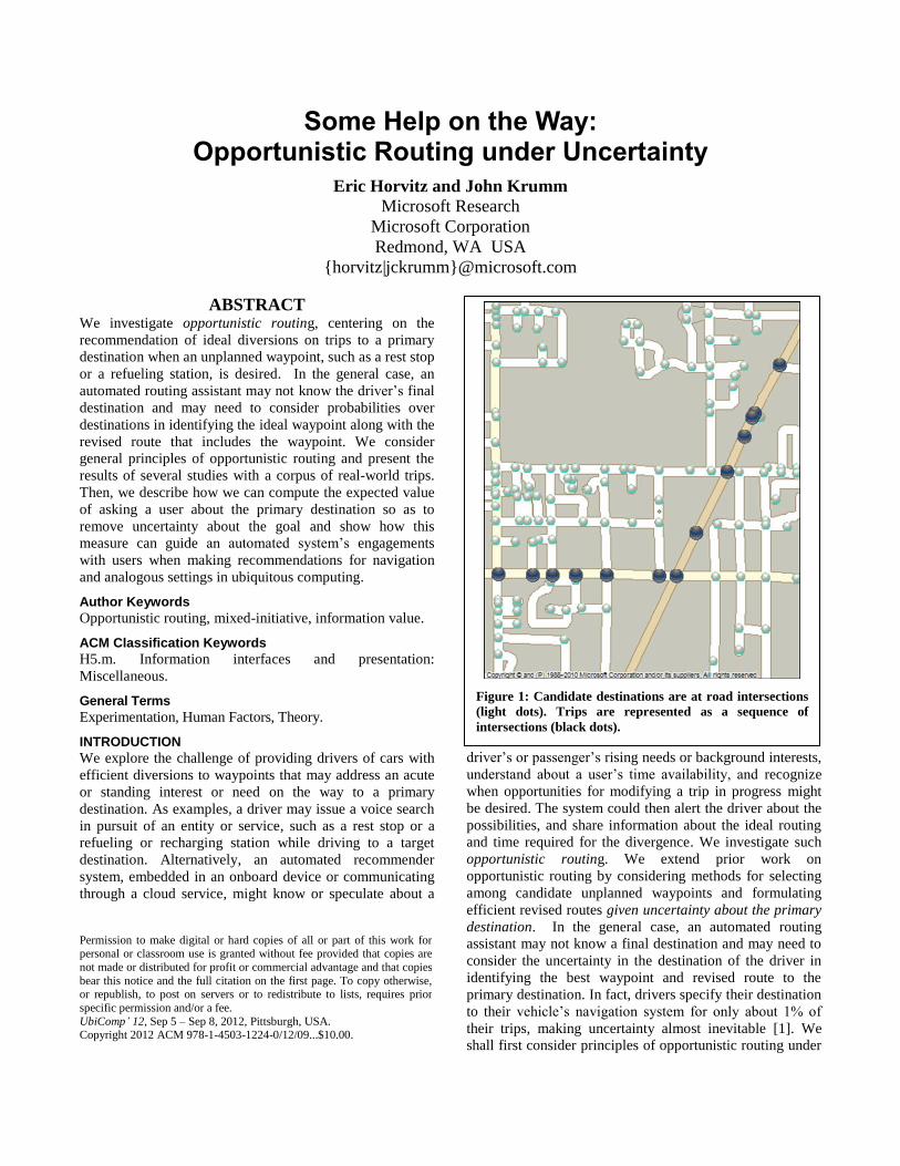
Figure 1: Candidate destinations are at road intersections

(light dots). Trips are represented as a sequence of

intersections (black dots).

uncertainty. Then we introduce methods for computing the

expected value of gaining additional information about the

primary destination. We discuss how this computation can

be harnessed to guide decisions about the value of asking

drivers to resolve a system’s uncertainty about the ultimate

destinations—versus providing recommendations on

waypoint candidates in an autonomous manner.

RELATED WORK

The problem of mobile opportunistic routing was

introduced by Horvitz, Koch, and Subramani in [2]. The

work presents methods for opportunistic routing and

describes a prototype named Mobile Commodities. The

system receives queries or automatically identifies needs

for accessing goods or services during a trip to primary

destination. Standing goals, such as “search for a gas

station when fuel tank is less than 10 percent full,” can be

encoded in the system. The prototype continues to perform

cost-benefit analyses as it speculates about potentially

valuable waypoints and the time associated with investing

time in a diversion. While the project mentions the

challenge of handling uncertainty in destinations, the effort

focuses largely on cases where a known destination is input

to the system, and considers detailed modeling of the

uncertainty in the availability of a driver and the cost of

taking additional time to divert to and engage in an

opportunistic task, using Bayesian user models of the

context-sensitive cost of time (drawing upon information

from an online calendar and traffic). Inferences about the

cost of elapsed time are used in considerations of

introducing new waypoints or finding ideal solutions to

needs such as refueling a car based on a consideration of

the pricing and distance of fueling stations. Later related

work by Kamar, Horvitz, and Meek [3] explored multiple

challenges with electronic commerce in an opportunistic

routing setting and introduced an auction-centric system

named MC-Market. The prototype provides decisions

about offers and pricing for various goods and services

based on drivers’ locations, destination, and preferences,

and can initiate context-sensitive auctions on pricing of

services. Like the work before it, efforts on MC-Market

center largely on opportunistic routing in situations where

the primary destinations of drivers are known.

In this paper, we focus on opportunistic routing under

uncertain destinations. The work leverages prior work on

probabilistic predictions of a driver’s destination. The

problem of predicting destinations has been addressed by

other researchers. Marmasse and Schmandt [4] presented

experiments with a Bayes classifier, histogram matching,

and a hidden Markov model to match a partial route with

stored routes. Ashbrook and Starner [5] clustered GPS data

to find a person’s significant locations like home and work,

and then trained a Markov model to predict transitions

between these locations. Hariharan and Toyama present a

means of clustering GPS points and then use a Markov

model to characterize transitions [6]. Liao et al. [7] and

Patterson et al. [8] describe probabilistic models for route

prediction, trained from observations on individuals.

Besides routes, their techniques can infer the person’s mode

of transportation. The Predestination algorithm by Krumm

and Horvitz predicts destinations based partially on past

behavior, but also allows for predictions at previously

unvisited locations [9]. Ziebart et al. train a location

prediction algorithm from GPS observations of 25 taxi

drivers [10]. Their algorithm reasons about route decisions

in context and gives predictions for the driver’s next turn,

their route to a given destination, and their next destination

given a partially observed trip. The NextPlace system not

only predicts destinations, but arrival times [11]. Filev et al.

present a fuzzy Markov model for predicting previously

visited destinations based on the previous destination, the

day of the week, and the time of day [12].

While our technique recommends slight modifications to a

driver’s existing route, other work has concentrated on

recommending entire routes, such as the T-Drive system by

Yuan et al. [13]. The same group has looked at helping taxi

drivers find their next passenger [14] and travel

recommendations based on GPS traces [15]. Also related is

the work of Zhang et al. who learn a user’s important

locations and routes [16].

DESTINATION PREDICTION

Identifying the optimal waypoint, and associated diversion

introduced to a trip, requires knowledge of the driver’s

destination. Although a driver may sometimes provide a

destination to a vehicle’s navigation system, this happens

rarely. Thus, we take as a central focus the identification of

ideal waypoints under uncertainty in a driver’s destination.

To compute probabilities over destinations, we employ a

destination prediction algorithm derived as a modification

of the methodology described in [17]. The technique is

based on the observation and expectation that drivers drive

efficiently toward their destination. The method computes

destination probabilities ( ) for destinations contained

in a set of candidate destinations , i.e. . In the

version of the algorithm we shall use in studies, the

candidate destinations consist of all road intersections

within 60 minutes driving time from the start of the trip.

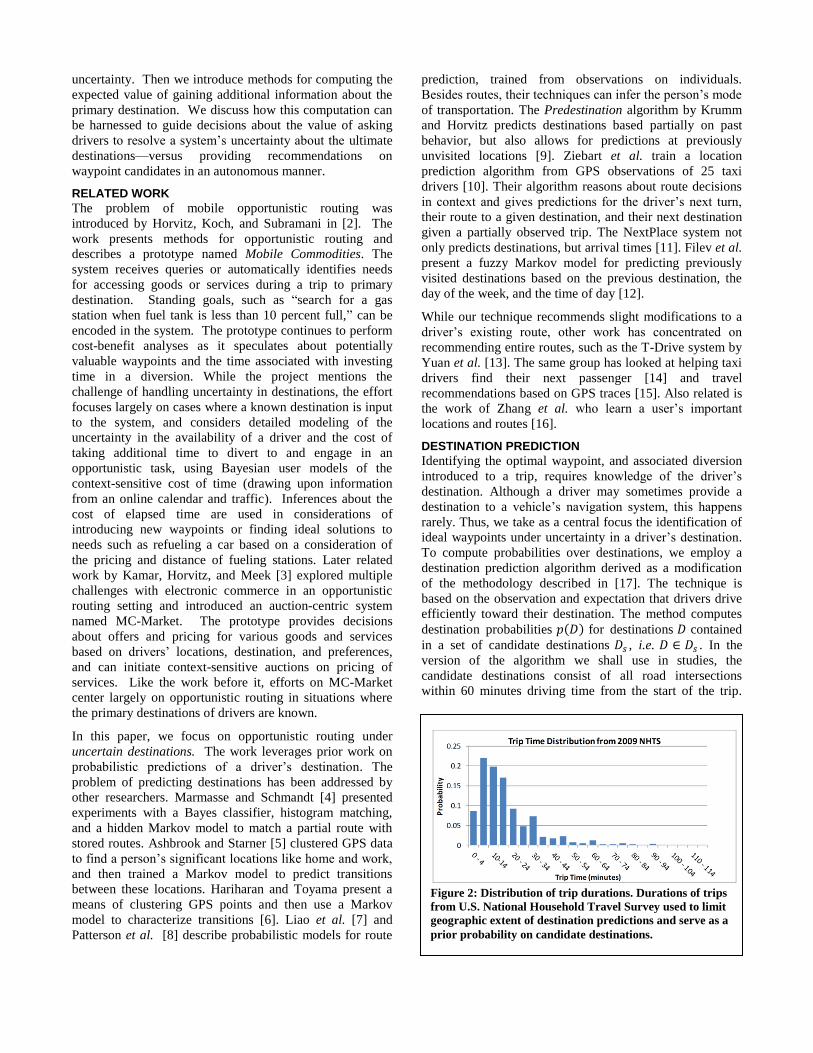
Figure 2: Distribution of trip durations. Durations of trips

from U.S. National Household Travel Survey used to limit

geographic extent of destination predictions and serve as a

prior probability on candidate destinations.

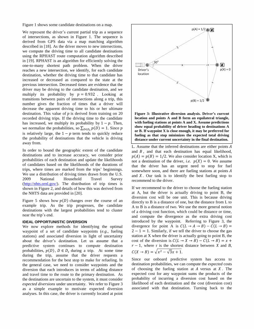
Figure 1 shows some candidate destinations on a map.

We represent the driver’s current partial trip as a sequence

of intersections, as shown in Figure 1. The sequence is

derived from GPS data via a map matching algorithm

described in [18]. As the driver moves to new intersections,

we compute the driving time to all candidate destinations

using the RPHAST route computation algorithm described

in [19]. RPHAST is an algorithm for efficiently solving the

one-to-many shortest path problem. When the driver

reaches a new intersection, we identify, for each candidate

destination, whether the driving time to that candidate has

increased or decreased as compared to the state at the

previous intersection. Decreased times are evidence that the

driver may be driving to the candidate destination, and we

multiply its probability by . Looking at

transitions between pairs of intersections along a trip, this

number gives the fraction of times that a driver will

decrease the apparent driving time to his or her ultimate

destination. This value of is derived from training on 20

recorded driving trips. If the driving time to the candidate

has increased, we multiply its probability by . Then,

we normalize the probabilities, so ∑ ( ) . Since

is relatively large, the term tends to quickly reduce

the probability of destinations that the vehicle is driving

away from.

In order to bound the geographic extent of the candidate

destinations and to increase accuracy, we consider prior

probabilities of each destination and update the likelihoods

of candidates based on the likelihoods of the durations of

trips, where times are marked from the trips’ beginnings.

We use a distribution of driving times drawn from the U.S.

2009 National Household Travel Survey

(http://nhts.ornl.gov/). The distribution of trip times is

shown in Figure 2, and details of how this was derived from

the NHTS data are provided in [20].

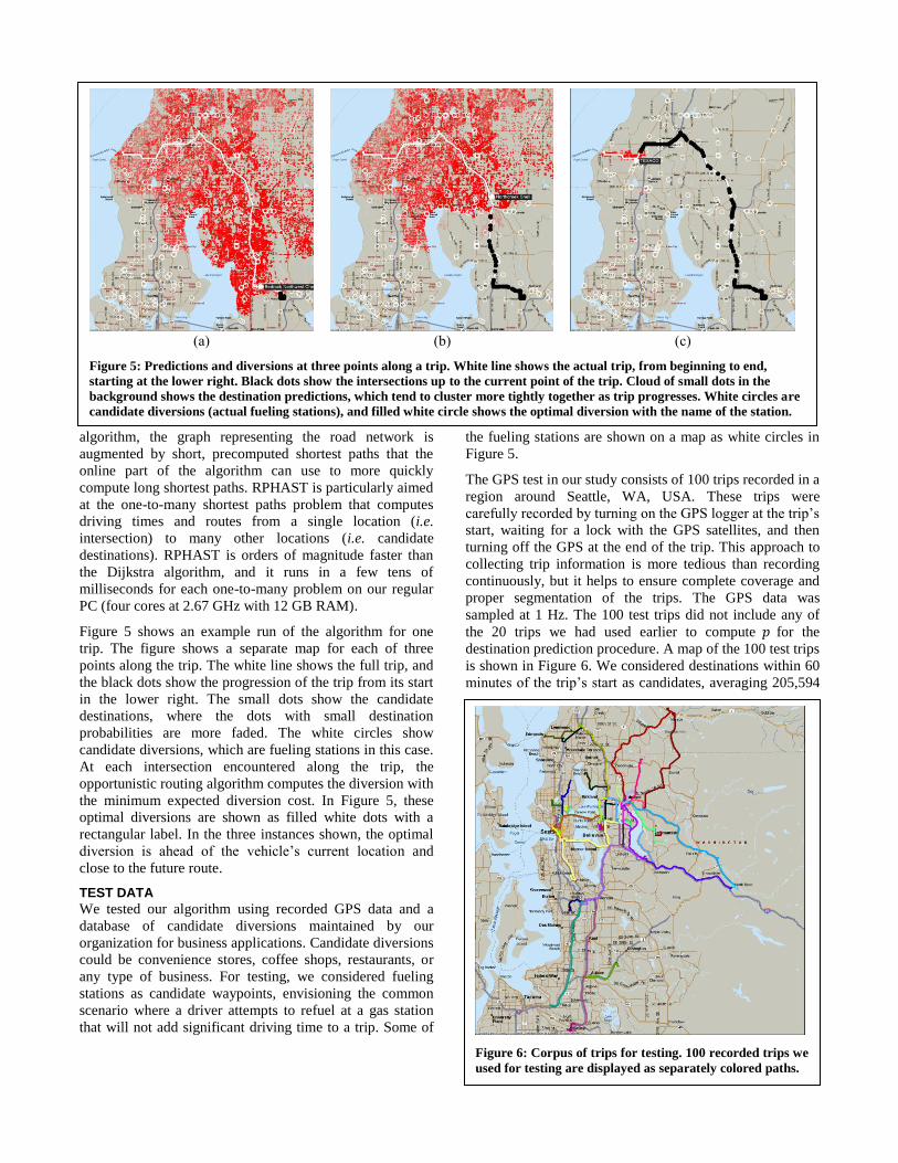
Figure 5 shows how ( ) changes over the course of an

example trip. As the trip progresses, the candidate

destinations with the largest probabilities tend to cluster

near the trip’s end.

IDEAL OPPORTUNISTIC DIVERSION

We now explore methods for identifying the optimal

waypoint of a set of candidate waypoints (e.g., fueling

stations) and associated diversion in light of uncertainty

about the driver’s destination. Let us assume that a

predictive system continues to compute destination

probabilities, ( ) , during a trip. At some time

during the trip, assume that the driver requests a

recommendation for the best stop to make for refueling. In

the general case, we need to consider waypoints and the

diversion that each introduces in terms of adding distance

and travel time to the route to the primary destination. As

the destinations are uncertain to the system, it must consider

expected diversions under uncertainty. We refer to Figure 3

as a simple example to motivate expected diversion

analyses. In this case, the driver is currently located at point

L. Assume that the inferred destinations are either points

and , and that each destination has equal likelihood,

( ) ( ) . We also consider location X, which is

not a destination of the driver, i.e. ( ) . We assume

that the driver has an urgent need to stop for fuel

somewhere soon, and there are fueling stations at points

and . Our task is to identify the best fueling stop to

recommend to the driver.

If we recommend to the driver to choose the fueling station

at A, but the driver is actually driving to point B, the

diversion cost will be one unit. This is because driving

directly to B is a distance of one, but the distance from L to

A to B is a distance of two. We use the more general notion

of a driving cost function, which could be distance or time,

and compute the divergence as the extra driving cost

introduced by the waypoint. Referring to Figure 3, the

divergence for point A is ( ) ( ) . Similarly, if we tell the driver to choose the gas

station at X when the driver is actually going to point B, the

cost of the diversion is ( ) ( ) , where r is the shortest distance between X and B,

( ) √ √ .

Since our onboard predictive system has access to

destination probabilities, we can compute the expected costs

of choosing the fueling station at versus at . The

expected cost for any waypoint sums the products of the

probability of incurring a diversion cost based on the

likelihood of each destination and the cost (diversion cost)

associated with that destination. Turning back to the

Figure 3: Illustrative diversion analysis. Driver’s current

location and points A and B form an equilateral triangle,

with fueling stations at points A and X. Assume predictions

show equal probability of driver heading to destinations A

or B. If waypoint X is close enough, it may be preferred for

fueling as that stop minimizes the expected total driving

distance under current uncertainty in the final destination.

illustrative example, the expected cost of choosing the gas

station at is thus,

( )[ ( ) ( )]

( )[ ( ) ( )]

( )[ ( ) ( )]

[ ]

[ ]

[ ]

We can compute the expected cost of choosing the gas

station at in a similar way:

( )[ ( ) ( )]

( )[ ( ) ( )]

( )[ ( ) ( )]

[ ]

[ ]

[ ]

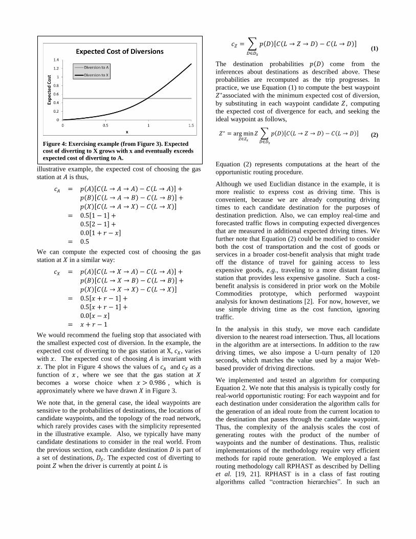
We would recommend the fueling stop that associated with

the smallest expected cost of diversion. In the example, the

expected cost of diverting to the gas station at , , varies

with . The expected cost of choosing is invariant with

. The plot in Figure 4 shows the values of and as a

function of , where we see that the gas station at

becomes a worse choice when , which is

approximately where we have drawn in Figure 3.

We note that, in the general case, the ideal waypoints are

sensitive to the probabilities of destinations, the locations of

candidate waypoints, and the topology of the road network,

which rarely provides cases with the simplicity represented

in the illustrative example. Also, we typically have many

candidate destinations to consider in the real world. From

the previous section, each candidate destination is part of

a set of destinations, . The expected cost of diverting to

point when the driver is currently at point is

∑ ( )[ ( ) ( )]

(1)

The destination probabilities ( ) come from the

inferences about destinations as described above. These

probabilities are recomputed as the trip progresses. In

practice, we use Equation (1) to compute the best waypoint

associated with the minimum expected cost of diversion,

by substituting in each waypoint candidate , computing

the expected cost of divergence for each, and seeking the

ideal waypoint as follows,

∑ ( )[ ( ) ( )]

(2)

Equation (2) represents computations at the heart of the

opportunistic routing procedure.

Although we used Euclidian distance in the example, it is

more realistic to express cost as driving time. This is

convenient, because we are already computing driving

times to each candidate destination for the purposes of

destination prediction. Also, we can employ real-time and

forecasted traffic flows in computing expected divergences

that are measured in additional expected driving times. We

further note that Equation (2) could be modified to consider

both the cost of transportation and the cost of goods or

services in a broader cost-benefit analysis that might trade

off the distance of travel for gaining access to less

expensive goods, e.g., traveling to a more distant fueling

station that provides less expensive gasoline. Such a cost-

benefit analysis is considered in prior work on the Mobile

Commodities prototype, which performed waypoint

analysis for known destinations [2]. For now, however, we

use simple driving time as the cost function, ignoring

traffic.

In the analysis in this study, we move each candidate

diversion to the nearest road intersection. Thus, all locations

in the algorithm are at intersections. In addition to the raw

driving times, we also impose a U-turn penalty of 120

seconds, which matches the value used by a major Web-

based provider of driving directions.

We implemented and tested an algorithm for computing

Equation 2. We note that this analysis is typically costly for

real-world opportunistic routing: For each waypoint and for

each destination under consideration the algorithm calls for

the generation of an ideal route from the current location to

the destination that passes through the candidate waypoint.

Thus, the complexity of the analysis scales the cost of

generating routes with the product of the number of

waypoints and the number of destinations. Thus, realistic

implementations of the methodology require very efficient

methods for rapid route generation. We employed a fast

routing methodology call RPHAST as described by Delling

et al. [19, 21]. RPHAST is in a class of fast routing

algorithms called “contraction hierarchies”. In such an

Figure 4: Exercising example (from Figure 3). Expected

cost of diverting to X grows with x and eventually exceeds

expected cost of diverting to A.

algorithm, the graph representing the road network is

augmented by short, precomputed shortest paths that the

online part of the algorithm can use to more quickly

compute long shortest paths. RPHAST is particularly aimed

at the one-to-many shortest paths problem that computes

driving times and routes from a single location (i.e.

intersection) to many other locations (i.e. candidate

destinations). RPHAST is orders of magnitude faster than

the Dijkstra algorithm, and it runs in a few tens of

milliseconds for each one-to-many problem on our regular

PC (four cores at 2.67 GHz with 12 GB RAM).

Figure 5 shows an example run of the algorithm for one

trip. The figure shows a separate map for each of three

points along the trip. The white line shows the full trip, and

the black dots show the progression of the trip from its start

in the lower right. The small dots show the candidate

destinations, where the dots with small destination

probabilities are more faded. The white circles show

candidate diversions, which are fueling stations in this case.

At each intersection encountered along the trip, the

opportunistic routing algorithm computes the diversion with

the minimum expected diversion cost. In Figure 5, these

optimal diversions are shown as filled white dots with a

rectangular label. In the three instances shown, the optimal

diversion is ahead of the vehicle’s current location and

close to the future route.

TEST DATA

We tested our algorithm using recorded GPS data and a

database of candidate diversions maintained by our

organization for business applications. Candidate diversions

could be convenience stores, coffee shops, restaurants, or

any type of business. For testing, we considered fueling

stations as candidate waypoints, envisioning the common

scenario where a driver attempts to refuel at a gas station

that will not add significant driving time to a trip. Some of

the fueling stations are shown on a map as white circles in

Figure 5.

The GPS test in our study consists of 100 trips recorded in a

region around Seattle, WA, USA. These trips were

carefully recorded by turning on the GPS logger at the trip’s

start, waiting for a lock with the GPS satellites, and then

turning off the GPS at the end of the trip. This approach to

collecting trip information is more tedious than recording

continuously, but it helps to ensure complete coverage and

proper segmentation of the trips. The GPS data was

sampled at 1 Hz. The 100 test trips did not include any of

the 20 trips we had used earlier to compute for the

destination prediction procedure. A map of the 100 test trips

is shown in Figure 6. We considered destinations within 60

minutes of the trip’s start as candidates, averaging 205,594

(a) (b) (c)

Figure 5: Predictions and diversions at three points along a trip. White line shows the actual trip, from beginning to end,

starting at the lower right. Black dots show the intersections up to the current point of the trip. Cloud of small dots in the

background shows the destination predictions, which tend to cluster more tightly together as trip progresses. White circles are

candidate diversions (actual fueling stations), and filled white circle shows the optimal diversion with the name of the station.

Figure 6: Corpus of trips for testing. 100 recorded trips we

used for testing are displayed as separately colored paths.

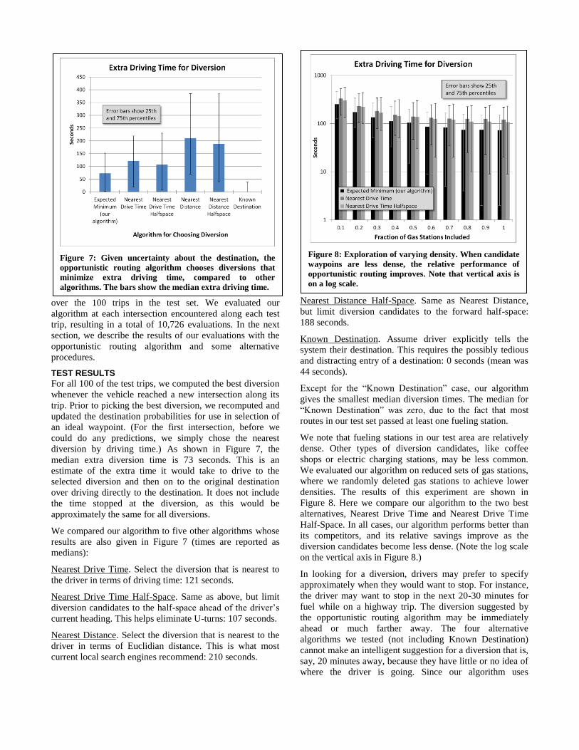
over the 100 trips in the test set. We evaluated our

algorithm at each intersection encountered along each test

trip, resulting in a total of 10,726 evaluations. In the next

section, we describe the results of our evaluations with the

opportunistic routing algorithm and some alternative

procedures.

TEST RESULTS

For all 100 of the test trips, we computed the best diversion

whenever the vehicle reached a new intersection along its

trip. Prior to picking the best diversion, we recomputed and

updated the destination probabilities for use in selection of

an ideal waypoint. (For the first intersection, before we

could do any predictions, we simply chose the nearest

diversion by driving time.) As shown in Figure 7, the

median extra diversion time is 73 seconds. This is an

estimate of the extra time it would take to drive to the

selected diversion and then on to the original destination

over driving directly to the destination. It does not include

the time stopped at the diversion, as this would be

approximately the same for all diversions.

We compared our algorithm to five other algorithms whose

results are also given in Figure 7 (times are reported as

medians):

Nearest Drive Time. Select the diversion that is nearest to

the driver in terms of driving time: 121 seconds.

Nearest Drive Time Half-Space. Same as above, but limit

diversion candidates to the half-space ahead of the driver’s

current heading. This helps eliminate U-turns: 107 seconds.

Nearest Distance. Select the diversion that is nearest to the

driver in terms of Euclidian distance. This is what most

current local search engines recommend: 210 seconds.

Nearest Distance Half-Space. Same as Nearest Distance,

but limit diversion candidates to the forward half-space:

188 seconds.

Known Destination. Assume driver explicitly tells the

system their destination. This requires the possibly tedious

and distracting entry of a destination: 0 seconds (mean was

44 seconds).

Except for the “Known Destination” case, our algorithm

gives the smallest median diversion times. The median for

“Known Destination” was zero, due to the fact that most

routes in our test set passed at least one fueling station.

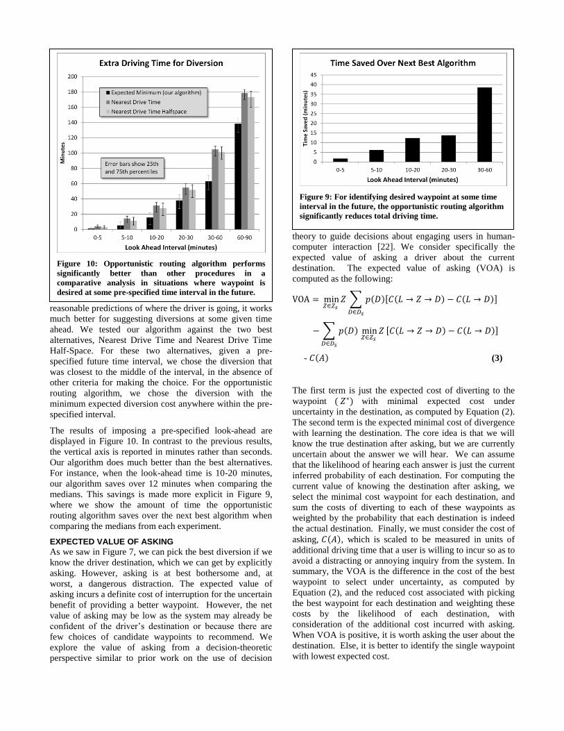
We note that fueling stations in our test area are relatively

dense. Other types of diversion candidates, like coffee

shops or electric charging stations, may be less common.

We evaluated our algorithm on reduced sets of gas stations,

where we randomly deleted gas stations to achieve lower

densities. The results of this experiment are shown in

Figure 8. Here we compare our algorithm to the two best

alternatives, Nearest Drive Time and Nearest Drive Time

Half-Space. In all cases, our algorithm performs better than

its competitors, and its relative savings improve as the

diversion candidates become less dense. (Note the log scale

on the vertical axis in Figure 8.)

In looking for a diversion, drivers may prefer to specify

approximately when they would want to stop. For instance,

the driver may want to stop in the next 20-30 minutes for

fuel while on a highway trip. The diversion suggested by

the opportunistic routing algorithm may be immediately

ahead or much farther away. The four alternative

algorithms we tested (not including Known Destination)

cannot make an intelligent suggestion for a diversion that is,

say, 20 minutes away, because they have little or no idea of

where the driver is going. Since our algorithm uses

Figure 7: Given uncertainty about the destination, the

opportunistic routing algorithm chooses diversions that

minimize extra driving time, compared to other

algorithms. The bars show the median extra driving time.

Figure 8: Exploration of varying density. When candidate

waypoins are less dense, the relative performance of

opportunistic routing improves. Note that vertical axis is

on a log scale.

reasonable predictions of where the driver is going, it works

much better for suggesting diversions at some given time

ahead. We tested our algorithm against the two best

alternatives, Nearest Drive Time and Nearest Drive Time

Half-Space. For these two alternatives, given a pre-

specified future time interval, we chose the diversion that

was closest to the middle of the interval, in the absence of

other criteria for making the choice. For the opportunistic

routing algorithm, we chose the diversion with the

minimum expected diversion cost anywhere within the pre-

specified interval.

The results of imposing a pre-specified look-ahead are

displayed in Figure 10. In contrast to the previous results,

the vertical axis is reported in minutes rather than seconds.

Our algorithm does much better than the best alternatives.

For instance, when the look-ahead time is 10-20 minutes,

our algorithm saves over 12 minutes when comparing the

medians. This savings is made more explicit in Figure 9,

where we show the amount of time the opportunistic

routing algorithm saves over the next best algorithm when

comparing the medians from each experiment.

EXPECTED VALUE OF ASKING

As we saw in Figure 7, we can pick the best diversion if we

know the driver destination, which we can get by explicitly

asking. However, asking is at best bothersome and, at

worst, a dangerous distraction. The expected value of

asking incurs a definite cost of interruption for the uncertain

benefit of providing a better waypoint. However, the net

value of asking may be low as the system may already be

confident of the driver’s destination or because there are

few choices of candidate waypoints to recommend. We

explore the value of asking from a decision-theoretic

perspective similar to prior work on the use of decision

theory to guide decisions about engaging users in human-

computer interaction [22]. We consider specifically the

expected value of asking a driver about the current

destination. The expected value of asking (VOA) is

computed as the following:

∑ ( )[ ( ) ( )]

∑ ( )

[ ( ) ( )]

- ( ) (3)

The first term is just the expected cost of diverting to the

waypoint ( ) with minimal expected cost under

uncertainty in the destination, as computed by Equation (2).

The second term is the expected minimal cost of divergence

with learning the destination. The core idea is that we will

know the true destination after asking, but we are currently

uncertain about the answer we will hear. We can assume

that the likelihood of hearing each answer is just the current

inferred probability of each destination. For computing the

current value of knowing the destination after asking, we

select the minimal cost waypoint for each destination, and

sum the costs of diverting to each of these waypoints as

weighted by the probability that each destination is indeed

the actual destination. Finally, we must consider the cost of

asking, ( ), which is scaled to be measured in units of

additional driving time that a user is willing to incur so as to

avoid a distracting or annoying inquiry from the system. In

summary, the VOA is the difference in the cost of the best

waypoint to select under uncertainty, as computed by

Equation (2), and the reduced cost associated with picking

the best waypoint for each destination and weighting these

costs by the likelihood of each destination, with

consideration of the additional cost incurred with asking.

When VOA is positive, it is worth asking the user about the

destination. Else, it is better to identify the single waypoint

with lowest expected cost.

Figure 9: For identifying desired waypoint at some time

interval in the future, the opportunistic routing algorithm

significantly reduces total driving time.

Figure 10: Opportunistic routing algorithm performs

significantly better than other procedures in a

comparative analysis in situations where waypoint is

desired at some pre-specified time interval in the future.

We note that over a trip the point-wise VOA can be

changing as the value of each term can shift based on

changes in the probabilities inferred about different ultimate

destinations, and the changing details of the geospatial

structure of waypoints and the topology of the road network

relative to the current location of the car. Also, beyond a

driver’s preferences about being asked about destinations,

the cost of such an interaction can change based on several

contextual factors, including whether a driver is currently

speaking with a passenger and the complexity of driving.

Studies in driving simulators have demonstrated the

existence of a task-dependent microstructure of the

interaction of human cognition and driving complexity, and

the influence of different mixes of road complexity and

cognitive tasks (e.g., introduced in phone conversations) on

driving safety [23]. In practice a proactive system might

monitor the value of asking and if positive defer engaging

the user until a better time. Other studies of bounded

deferral of notifications and engagement are relevant to this

task [24].

We performed a study with the same test corpus of 100

recorded GPS trips aimed at exploring the expected value

of asking using Equation (3) to compute the value of

asking. We set ( ) here for simplicity. We found that

the median cost saved by asking is 16 seconds. The 75th

percentile of savings is 99 seconds, and maximum savings

is about 23 minutes. The relatively low median shows that

our algorithm is doing a good job recommending a

waypoint, based on predictions. However, the value of

asking can be high, so it can be valuable to ask about the

destination.

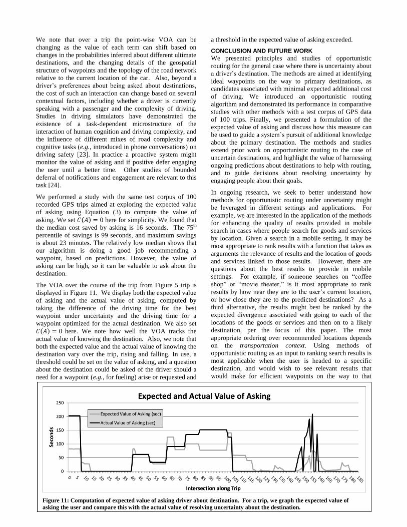
The VOA over the course of the trip from Figure 5 trip is

displayed in Figure 11. We display both the expected value

of asking and the actual value of asking, computed by

taking the difference of the driving time for the best

waypoint under uncertainty and the driving time for a

waypoint optimized for the actual destination. We also set

( ) here. We note how well the VOA tracks the

actual value of knowing the destination. Also, we note that

both the expected value and the actual value of knowing the

destination vary over the trip, rising and falling. In use, a

threshold could be set on the value of asking, and a question

about the destination could be asked of the driver should a

need for a waypoint (e.g., for fueling) arise or requested and

a threshold in the expected value of asking exceeded.

CONCLUSION AND FUTURE WORK

We presented principles and studies of opportunistic

routing for the general case where there is uncertainty about

a driver’s destination. The methods are aimed at identifying

ideal waypoints on the way to primary destinations, as

candidates associated with minimal expected additional cost

of driving. We introduced an opportunistic routing

algorithm and demonstrated its performance in comparative

studies with other methods with a test corpus of GPS data

of 100 trips. Finally, we presented a formulation of the

expected value of asking and discuss how this measure can

be used to guide a system’s pursuit of additional knowledge

about the primary destination. The methods and studies

extend prior work on opportunistic routing to the case of

uncertain destinations, and highlight the value of harnessing

ongoing predictions about destinations to help with routing,

and to guide decisions about resolving uncertainty by

engaging people about their goals.

In ongoing research, we seek to better understand how

methods for opportunistic routing under uncertainty might

be leveraged in different settings and applications. For

example, we are interested in the application of the methods

for enhancing the quality of results provided in mobile

search in cases where people search for goods and services

by location. Given a search in a mobile setting, it may be

most appropriate to rank results with a function that takes as

arguments the relevance of results and the location of goods

and services linked to those results. However, there are

questions about the best results to provide in mobile

settings. For example, if someone searches on “coffee

shop” or “movie theater,” is it most appropriate to rank

results by how near they are to the user’s current location,

or how close they are to the predicted destinations? As a

third alternative, the results might best be ranked by the

expected divergence associated with going to each of the

locations of the goods or services and then on to a likely

destination, per the focus of this paper. The most

appropriate ordering over recommended locations depends

on the transportation context. Using methods of

opportunistic routing as an input to ranking search results is

most applicable when the user is headed to a specific

destination, and would wish to see relevant results that

would make for efficient waypoints on the way to that

Figure 11: Computation of expected value of asking driver about destination. For a trip, we graph the expected value of

asking the user and compare this with the actual value of resolving uncertainty about the destination.

destination. Proximity-based ranking may be best for the

transportation contexts where driver and passengers are

either casually exploring a city or are leaving or planning to

leave their homes and offices to head directly to the specific

location before returning back. Inferences about users’

transportation contexts may be feasible based on such rich

attributes as location and velocity data, and streams of

queries over time.

ACKNOWLEDGMENTS

We thank Daniel Delling for his assistance with using

efficient routing routines.

REFERENCES

1. Krumm, J., Where Will They Turn: Predicting Turn

Proportions At Intersections. Personal and Ubiquitous

Computing, 2010. 14(7): p. 591-599.

2. Horvitz, E., P. Koch, and M. Subramani, Mobile

Opportunistic Planning: Methods and Models, in 11th

international conference on User Modeling (UM 2007).

2007. p. 228-237.

3. Kamar, E., E. Horvitz, and C. Meek, Mobile

Opportunistic Commerce: Mechanisms, Architecture,

and Application, in International Conference on

Autonomous Agents and Multiagent Systems (AAMAS

2008). 2008: Estoril, Portugal.

4. Marmasse, N. and C. Schmandt, A User-Centered

Location Model. Personal and Ubiquitous Computing,

2002(6): p. 318-321.

5. Ashbrook, D. and T. Starner, Using GPS to Learn

Significant Locations and Predict Movement across

Multiple Users. Personal and Ubiquitous Computing,

2003. 7(5): p. 275-286.

6. Hariharan, R. and K. Toyama. Project Lachesis:

Parsing and Modeling Location Histories. in

Geographic Information Science: Third International

Conference, GIScience 2004. 2004. Adelphi, MD, USA:

Springer-Verlag GmbH.

7. Liao, L., D. Fox, and H. Kautz. Learning and Inferring

Transportation Routines. in Proceedings of the 19th

National Conference on Artificial Intelligence (AAAI

2004). 2004. San Jose, CA, USA.

8. Patterson, D.J., et al., Inferring High-Level Behavior

from Low-Level Sensors, in UbiComp 2003: Ubiquitous

Computing. 2003: Seattle, WA USA. p. 73-89.

9. Krumm, J. and E. Horvitz, Predestination: Inferring

Destinations from Partial Trajectories, in UbiComp

2006: Ubiquitous Computing. 2006: Orange County,

CA USA. p. 243-260.

10. Ziebart, B.D., et al., Navigate Like a Cabbie:

Probabilistic Reasoning from Observed Context-Aware

Behavior, in Tenth International Conference on

Ubiquitous Computing (UbiComp 2008). 2008: Seoul,

South Korea. p. 322-331.

11. Scellato, S., et al., NextPlace: A Spatio-temporal

Prediction Framework for Pervasive Systems, in 9th

International Conference on Pervasive Computing

(Pervasive 2011). 2011: San Francisco, CA USA.

12. Filev, D., et al., Contextual On-Board Learning and

Prediction of Vehicle Destinations, in 2011 IEEE

Symposium on Computational Intelligence in Vehicles

and Transportation Systems (CIVTS). 2011: Paris,

France. p. 87-91.

13. Yuan, J., et al., T-Drive: Driving Directions Based on

Taxi Trajectories, in 18th ACM SIGSPATIAL

International Symposium on Advances in Geographic

Information Systems (GIS). 2010, ACM: San Jose, CA

USA.

14. Yuan, J., et al., Where to Find My Next Passenger?, in

13th International Conference on Ubiquitous

Computing (UbiComp 2011). 2011, ACM: Beijing,

China.

15. Zheng, Y. and X. Xie, Learning Travel

Recommendations from User-Generated GPS Traces.

ACM Transactions on Intelligent Systems and

Technology (TIST) 2011. 2(1).

16. Zhang, K., et al., Adaptive Learning of Semantic

Locations and Routes, in 3rd International Symposium

in Location- and Context-Awareness (LoCA). 2007,

Springer: Oberpfaffenhofen, Germany. p. 193-210.

17. Krumm, J., Real Time Destination Prediction Based on

Efficient Routes, in Society of Automotive Engineers

(SAE) 2006 World Congress. 2006: Detroit, Michigan,

USA.

18. Newson, P. and J. Krumm, Hidden Markov Map

Matching Through Noise and Spaseness, in 17th ACM

SIGSPATIAL Conference on Advances in Geographic

Information Systems (GIS '09). 2009: Seattle, WA

USA. p. 336-343.

19. Delling, D., A.V. Goldberg, and R.F. Werneck, Faster

Batched Shortest Paths in Road Networks, in 11th

Workshop on Algorithmic Approaches for

Transportation Modeling, Optimization, and Systems

(ATMOS'11). 2011: Saarbruecken, Germany.

20. Krumm, J., How People Use Their Vehicles: Statistics

from the 2009 National Household Travel Survey, in

Society of Automotive Engineers (SAE) 2012 World

Congress. 2012: Detroit, MI USA.

21. Delling, D., et al., PHAST: Hardware-accelerated

shortest path trees Journal of Parallel and Distributed

Computing, 2012.

22. Horvitz, E., Principles of Mixed-Initiative User

Interfaces, in SIGCHI Conference on Human Factors in

Computing Systems (CHI 1999). 1999, ACM:

Pittsburgh, Pennsylvania, USA.

23. Iqbal, S., Y.-C. Ju, and E. Horvitz, Cars, Calls and

Cognition: Investigating Driving and Divided Attention,

in 2010 ACM Conference on Human Factors in

Computing Systems (CHI 2010). 2010: Atlanta,

Georgia, USA.

24. Horvitz, E., J. Apacible, and M. Subramani, Balancing

Awareness and Interruption: Investigation of

Notification Deferral Policies, in Tenth Conference on

User Modeling (UM 2005). 2005: Edinburgh, Scotland.