verification of mechanistic-empirical pavement
TRANSCRIPT

Verification of Mechanistic-Empirical Pavement Deterioration Models Based on Field Evaluation
of In-Service Pavements
Carlos Rafael Gramajo
Thesis Submitted to the Faculty of Virginia Polytechnic Institute and State University
in Partial Fulfillment of the Requirements of the Degree of
Master of Science in Civil and Environmental Engineering
COMMITTEE MEMBERS:
Dr. Gerardo Flintsch, Chair
Dr. Imad Al-Qadi
Dr. Amara Loulizi
May 23, 2005
Blacksburg, Virginia
Keywords: Pavement evaluation, pavement structural capacity, backcalculation, mechanistic-
empirical design, performance prediction, pavement distresses

Verification of Mechanistic-Empirical Pavement Deterioration Models Based on Field Evaluation of In-Service Pavements
Carlos Rafael Gramajo
(Abstract)
This thesis focused on using a detailed structural evaluation of seven (three flexible and four
composite) high performance in-service pavements designated as high-priority routes to verify
the applicability of the Mechanistic Empirical (M-E) models to high performance pavements in
the Commonwealth of Virginia. The structural evaluation included: determination of layer
thicknesses (from cores, GPR and historical data), pavement condition assessment based on
visual survey, estimation of layer moduli from FWD analysis as well as material characterization.
One of the main objectives of this study was to utilize the results from the backcalculated moduli
in order to predict the performance of this group of pavement structures using the M-E Design
Guide Software. This allowed a quick verification of the performance prediction models used by
comparing their outcome with the current condition.
The in-depth structural evaluation of the three flexible and four composite pavements showed
that all the sites are structurally sound. The investigation also confirmed that the use of GPR to
determine layer thicknesses and the comparison with a minimum number of cores is a helpful
tool for pavement structural evaluation. Despite some difficulties performing the backcalculation
analysis for complex structures, the obtained results were considered reasonable and were
useful in estimating the current structural adequacy of the evaluated structures.
The comparison of the measured distresses with those predicted by the M-E Design Guide
software showed poor agreement. In general, the predicted distresses were higher than the
distresses actually measured. However, there was not enough evidence to determine whether
this is due to errors in the prediction models or software, or because of the use of defaults
material properties, specially for the AC layers. It must be noted that although an in-depth field
evaluation was performed, only Level 3 data was available for many of the input parameters.
The results suggest that significant calibration and validation will be required before
implementation of the M-E Design Guide.

iii
Acknowledgements I would like to express my gratitude to my advisor, Dr. Gerardo Flintsch, for all his support and
guidance during this graduate school experience. I would also like to express thanks to the
committee members, Dr. Imad Al-Qadi, of University of Illinois at Urbana Champaign, and Dr.
Amara Loulizi, of Virginia Tech.
I also owe thanks to my colleagues at Virginia Tech Transportation Institute for all their support
and friendship during these two years.
Finally, I would like to thank my family and friends for their trust and encouragement. I would
like to dedicate this thesis to my mother, Sonia, a friend who has always been there for me, and
who has made a lot of sacrifices to see her two sons succeed in life.

iv
Acronyms
AADTT Annual Average Daily Truck Traffic
AASHTO American Association of State Highway and Transportation Officials
AC Asphalt Concrete
ACI American Concrete Institute
ASCE American Society of Civil Engineers
ASTM American Society for Testing and Materials
ATB Asphalt Treated Base
CBR California Bearing Ratio
CCI Critical Condition Index
CRC Continuously Reinforced Concrete
CRCP Continuously Reinforced Concrete Pavement
CSL Chemically Stabilized Layer
CTA Cement Treated Aggregate
CV Coefficient of Variation
D Slab Thickness
Deff Effective Slab Thickness
DMI Distance Measurement Instrumentation
ESG Subgrade Modulus
FWD Falling Weight Deflectometer
FWD Falling Weight Deflectometer
GPR Ground Penetrating Radar
GSSI Geophysical Survey Systems, Inc
HMA Hot Mix Asphalt
IRI International Roughness Index
JCP Jointed Concrete Pavement
JCP Jointed Pavement Concrete
M-E Mechanistic-Empirical
MR Resilient Modulus
NCHRP National Cooperative Highway Research Program
NDT Non-Destructive Testing
PCC Portland Cement Concrete

v
PG Performance Grade
RMS Root Mean Square
SN Structural Number
SNeff Effective Structural Number
TAG Total Analysis Group
USCS Unified Soil Classification System
VDOT Virginia Department Of Transportation
vi
Table of Contents
Chapter 1 - INTRODUCTION ......................................................................................................... 1
1.1. Background.......................................................................................................................... 1
1.2. Problem Statement .............................................................................................................. 2
1.3. Research Objectives............................................................................................................ 2
1.4. Research Scope .................................................................................................................. 3
Chapter 2 - LITERATURE REVIEW............................................................................................... 4
2.1. Introduction .......................................................................................................................... 4
2.2. Pavement Evaluation........................................................................................................... 4
2.2.1. Structural Evaluation .................................................................................................... 5
2.2.2. Load Related Distresses .............................................................................................. 5
Fatigue Cracking................................................................................................................. 5
Fatigue Fracture in Chemically Stabilized Layers.............................................................. 5
Permanent Deformation (Rutting) ...................................................................................... 6
2.3. Destructive Structural Evaluation ........................................................................................ 7
2.4. Nondestructive Structural Evaluation .................................................................................. 8
2.4.1. Visual Survey................................................................................................................ 9
2.4.2. Ground Penetrating Radar (GPR).............................................................................. 11
2.4.3. Deflection Testing – Falling Weight Deflectometer (FWD) ........................................ 12
2.4.4. Moduli Backcalculation ............................................................................................... 14
Typical Moduli Values....................................................................................................... 14
Spatial Frequency ............................................................................................................. 15
2.5. M-E Design Analysis for Flexible Pavements ................................................................... 16
2.5.1. Design Inputs .............................................................................................................. 16
2.5.2. Critical Response Variables and Pavement Response Models ................................ 19
2.5.3. Incremental Distress and Trial Design Suitability ...................................................... 20
Chapter 3 - RESEARCH APPROACH ......................................................................................... 21
3.1. Data Collection................................................................................................................... 22
3.1.1. GPR Testing ............................................................................................................... 22
3.1.2. Visual/Video Survey ................................................................................................... 23
3.1.3. FWD Testing ............................................................................................................... 24
3.1.4. Coring/Boring.............................................................................................................. 25
3.2. Data Analysis Methodology ............................................................................................... 26
vii
3.2.1. Visual Distress Quantification..................................................................................... 26
3.2.2. Core Measurements and Material Characterization .................................................. 26
3.2.3. Layer Thickness Determination.................................................................................. 27
3.2.4. Deflection Analysis ..................................................................................................... 29
Deflection Variability Analysis........................................................................................... 29
Homogenous Sections...................................................................................................... 29
Layer Moduli Backcalculation ........................................................................................... 30
3.2.5. Determination of Effective Structural Capacity .......................................................... 30
Design (Original) Structural Number (SN)........................................................................ 31
Effective Structural Number (SNeff) from Condition Survey ............................................. 31
Effective Structural Number (SNeff) from NDT Evaluation................................................ 31
Design Subgrade Resilient Modulus (Design MR)............................................................ 32
Effective Modulus of the Pavement (Ep)........................................................................... 32
Effective Slab Thickness (Deff) .......................................................................................... 33
3.2.6. M-E Design Guide Software Verification.................................................................... 33
Input Variables .................................................................................................................. 35
Analysis Assumptions....................................................................................................... 35
Distress Models ................................................................................................................ 37
Chapter 4 - RESULTS AND DISCUSSION.................................................................................. 41
4.1. Visual Survey and Profile Measurements ......................................................................... 41
4.2. Backcalculation Results..................................................................................................... 42
4.3. Material Characterization................................................................................................... 46
4.4. Effective (current) Structural Capacity .............................................................................. 48
4.5. M-E Design Guide Software Results................................................................................. 50
4.5.1. Initial Construction ...................................................................................................... 50
4.5.2. After Overlay Predicted Performance ........................................................................ 52
Comparison of Measured and Predicted Performance.................................................... 53
Critical Distress Identification ........................................................................................... 58
4.6. M-E Design Guide Software Limitations and Troubleshooting ......................................... 59
Chapter 5 - FINDINGS AND CONCLUSIONS............................................................................. 61
5.1. Findings.............................................................................................................................. 61
5.2. Conclusions ....................................................................................................................... 62
Chapter 6 - RECOMMENDATIONS ............................................................................................. 64
Recommendations for Data Collection..................................................................................... 64

viii
Recommendation for Future Research .................................................................................... 65
References.................................................................................................................................... 66
Appendix A – Determination of Layer Thickness from Cores, GPR, and Historical Data........... 69
Appendix B – Homogeneous Sections Based on Cumulative Sums of Deflections ................... 73
Appendix C – Backcalculation Results ELMOD 5.1..................................................................... 78
Appendix D – M-E Design Software Output................................................................................. 83

ix
List of Figures
Figure 1. HMA Rutting .................................................................................................................... 6
Figure 2. Base/Subbase/Subgrade Rutting.................................................................................... 7
Figure 3. Core Sample.................................................................................................................... 8
Figure 4. Coring Machine and Core Extraction .............................................................................. 8
Figure 5. Pavement Structure Subjected to GPR Testing ........................................................... 11
Figure 6. FWD – Dynatest Model 8002....................................................................................... 12
Figure 7. Deformations of Pavement Subjected to Loading ........................................................ 13
Figure 8. Loading Plate and Geophones ..................................................................................... 13
Figure 9. Stress Zone of a Pavement Subjected to FWD Testing............................................... 15
Figure 10. Location of Evaluated Flexible and Composite Pavements Sites.............................. 21
Figure 11. Antenna Used for GPR Collection .............................................................................. 23
Figure 12. Digital Camera Used for Video Survey ....................................................................... 24
Figure 13. FWD Used by VDOT................................................................................................... 24
Figure 14: Raw GPR Data, Center of the Lane, Flexible Section................................................ 28
Figure 15. Homogeneous Sections Based on Cumulative Sum of Deflections – Site 2 ............. 30
Figure 16. Summary of Predicted Distresses from Construction to Overlay Year (Flexible) ...... 51
Figure 17. Summary of Predicted Distresses from Construction to Overlay Year (Composite) . 52
Figure 18. Predicted vs. Current Distresses – Surface-Down (longitudinal) Fatigue Cracking
(m/km) ................................................................................................................................... 53
Figure 19. Predicted vs. Current Distresses – Bottom-Up (alligator) Fatigue Cracking (% of Lane
Area)...................................................................................................................................... 54
Figure 20. Predicted vs. Current Distresses – Thermal Cracking (m/km) ................................... 55
Figure 21. Predicted vs. Current Distresses – Total Rutting (cm) .............................................. 56
Figure 22. Predicted vs. Current Distresses – IRI (m/km) .......................................................... 57
Figure 23. Summary of Existing Distresses in 2004 .................................................................... 59

x
List of Tables
Table 1. Distress Types and Levels for Assessing Flexible Pavement Structural Adequacy [1] 10
Table 2. Typical Stiffness Moduli for Different Materials.............................................................. 15
Table 3. Design Process Steps .................................................................................................... 16
Table 4. Description of Design Input Levels................................................................................. 17
Table 5. Allowable Distress Limits Recommended by the M-E Design Guide........................... 18
Table 6. Selected Pavement Sites ............................................................................................... 22
Table 7. Selection of Thicknesses Between Historical Data, GPR and Cores for Site 16
(Flexible) ............................................................................................................................... 29
Table 8. Summary of Pavement Structures Analyzed ................................................................. 34
Table 9. Input Parameters and Source of Information................................................................. 36
Table 10. Existing Surface Distresses and Profile Measurements.............................................. 41
Table 11. Adequacy Levels Based on Existing Distresses.......................................................... 42
Table 12. Deflection Variability Expressed in Terms of Coefficient of Variation (CV)................. 43
Table 13: Summary of Backcalculation Results for Flexible Pavements .................................... 44
Table 14. Summary of Backcalculation Results for Composite Pavements ............................... 45
Table 15. Comparison of Typical and Backcalculated Subgrade Moduli (ESG)........................... 46
Table 16. Comparison of Backcalculated and Laboratory Asphalt Moduli .................................. 47
Table 17. Comparison of Backcalculated and Laboratory CRCP Moduli................................... 48
Table 18. Effective Structural Number (SNeff) .............................................................................. 49
Table 19. Effective Slab Thickness (Deff)...................................................................................... 49
Table 20. Effective Slab Thickness (Deff)...................................................................................... 50

1
Chapter 1 - INTRODUCTION
1.1. Background This investigation focused on the use of structural evaluation results, specially Falling Weight
Deflectometer (FWD) and backcalculation, for supporting pavement analysis and design. The
Virginia Department of Transportation conducted a study for developing pavement designs for
high-priority routes based on current and past field experience. The investigation aimed at
identifying the necessary tools to effectively design pavement structures with a life span of 40
years or more. The first phase of this project included an in-depth field evaluation and analysis
of high performance in-service pavements designated as high-priority routes. In addition to
FWD testing, the field evaluation included Ground Penetrating Radar (GPR), and visual and
video surveys of the pavement surface. Additionally, a limited number of cores were taken from
each site and some of the core pits were used to perform subgrade boring. In total, eighteen
pavement sections were evaluated. These sections included flexible, composite, and rigid
(jointed and continuously reinforced) pavement structures. Seven of these sections were
selected to be part of this thesis; these sections included three flexible pavements and four
composite pavement structures.
Falling Weight Deflectometer (FWD) measurements were performed to determine the structural
condition of each of the test sites evaluated and to determine in-situ modulus of the various
layers. All tests were conducted using a Dynatest model 8002 FWD unit with nine sensing
transducers located at 0, 203, 305, 457, 610, 914, 1219, 1524 and 1829 mm (0, 8, 12, 18, 24,
36, 48, 60 and 72 in) from the center of the loading plate. The backcalculated moduli were
compared with moduli measured using laboratory tests for the pavement layers and estimated
based on geotechnical studies for the subgrade.
The results obtained from the backcalculation process were used as an input for modeling
pavement performance as presented in the “Guide for Mechanistic-Empirical Design of New and
Rehabilitated Pavement Structures” (hereafter referred to as M-E Design Guide) recently
developed under NCHRP 1-37A. The performance criteria of the M-E Design Guide includes
load-related distress prediction models that cover Asphalt Concrete (AC) surface-down and
bottom-up cracking, chemically stabilized layer fatigue fracture (for composite pavements),
permanent deformation (rutting) in asphalt layers, and permanent deformation in unbound

2
layers. The performance of the selected structures was predicted using the M-E Design Guide
(version 0.701) software1 and was compared to the distresses measured from the visual survey
results to verify the applicability of the models to the studied pavements.
In addition, the results from the Non-Destructive Evaluation (NDT) were used to estimate
effective (current) structural capacity of the pavements using the 1993 AASHTO Design
Methodology (in terms of structural number (SN) and equivalent slab thickness (D) for flexible
and composite pavements respectively). This allowed determining if the observed distresses
were compatible with the pavement’s effective structural capacity (SN and D) determined by this
procedure.
1.2. Problem Statement Nondestructive Testing (NDT) methods such as Falling Weight Deflectometer (FWD)
complemented with other evaluation techniques are commonly used to determine the structural
adequacy and condition of pavements. The results from a field evaluation, e.g. backcalculated
moduli, can be used as input parameters to predict the performance of a pavement structure as
a function of the accumulation of damage over time. The distress prediction models presented
in the M-E Design Software can be used to estimate pavement’s performance. However, the
applicability of these models to Virginia’s pavements has to be verified based on actual
pavement performance data.
1.3. Research Objectives This thesis focused on using a detailed structural evaluation of the pavement sections to verify
the applicability of the M-E models to high performance pavements in the Commonwealth of
Virginia. The structural evaluation included: determination of layer thicknesses (from cores,
GPR and historical data), pavement condition assessment based on visual survey, estimation of
layer moduli from FWD analysis, and material characterization. The main objective of this study
was to utilize the results from the backcalculated moduli in order to predict the performance of a
selected group of pavement structures using the M-E Design Software. This allowed a quick
1 Developed by ERES Division, Applied Research Associates and Arizona State University

3
verification of the performance prediction models used by comparing their outcome with the
current condition determined from the visual survey.
1.4. Research Scope This thesis is organized as follows. Chapter 2 contains a literature review regarding pavement
evaluation and mechanistic-empirical analysis of flexible pavements. Chapter 3 describes the
data collection and data analysis process. Chapter 4 discusses the results obtained from the
analyses performed. Chapter 5 includes the findings and conclusions, and Chapter 6 provides
recommendations for future research.

4
Chapter 2 - LITERATURE REVIEW
2.1. Introduction
The Report Card for America’s Infrastructure [2], recently published by the ASCE, showed that
more than sixty percent of the roads in the United States are in poor to mediocre condition,
which translates into unnecessary expenses to the drivers for maintenance, car repairs, traffic
congestions, accidents, etc. Therefore, there is a demand to improve highway conditions,
capacity, and safety, not only by building new roads, but also by maintaining the existing ones in
the best possible condition. Thus, it is important to evaluate the existing roadways to determine
their structural and functional capacity, as well as to understand the failure mechanisms,
enhance performance models, and take necessary actions to achieve the desired reliability.
2.2. Pavement Evaluation
The evaluation of pavements can be divided into two main groups: (1) Structural adequacy (load
related distresses) and (2) Functional adequacy (safety and rideability). Both types of
evaluations are used for pavement management. Since the condition of pavements
deteriorates over time, it is necessary to perform periodic evaluations to develop distress
history. This investigation focuses on the pavement structural evaluation using Falling Weight
Deflectometer (FWD).
Frequently, structural evaluation of pavements involves three sources of information: historical
data, destructive testing, and nondestructive testing (NDT). Nondestructive Testing (NDT)
methods are commonly supplemented with destructive testing techniques because experience
has shown that NDT techniques alone may not always provide a reasonable or accurate
characterization of the in situ material properties, particularly for the top pavement layers [10].
The most common pavement structural evaluation procedures will be discussed in the following
section.

5
2.2.1. Structural Evaluation The structural evaluation relates to the assessment of those properties and features that define
the response of the pavement to traffic loads. Results from the field evaluation should help
assessing the overall condition of the existing pavement and identifying pavement problems.
This is usually the first step in the process of pavement rehabilitation strategy selection.
2.2.2. Load Related Distresses The performance criteria of the M-E Design Guide includes the following load-related distress:
AC surface-down cracking (longitudinal cracking), AC bottom-up cracking (alligator cracking),
chemically stabilized layer fatigue fracture (only for composite pavements), permanent
deformation (rutting) in asphalt layers, and permanent deformation in unbound layers.
Fatigue Cracking
Fatigue cracking initiates as short longitudinal cracks that quickly spread in the wheelpath and
become interconnected following a pattern that resembles chicken wire or alligator skin. This
type of failure results from the repetitive bending of the HMA (Hot Mix Asphalt) layer while
subjected to traffic loads.
The bending action of the pavement layer results in flexural stresses that develop at the bottom
of the bound layer, this is why for more that 30 years it has been assumed that fatigue cracking
initiates at the bottom of the asphalt layer and propagates to the surface (bottom-up cracking).
Nevertheless, recent investigations have demonstrated that fatigue cracking may as well initiate
from the top and propagate down (top-down cracking) probably due to critical tensile and/or
shear stresses developed at the surface and caused by large contact pressures at the tire
edges-pavement interface [10], in combination with aged (oxidized or stiff) surface layers.
Fatigue Fracture in Chemically Stabilized Layers
Fatigue fracture in the underlying chemically stabilized base layers is a distress that needs to be
considered in composite pavements. Chemically stabilized layers are defined as high quality
base materials treated with materials such as lime, cement or flyash; the stiffness of these
layers can be reduced (and even lead to fatigue fracture) because of the development of
6
microcracks induced by repeated applications of traffic loading. This type of failure has a
significant impact on the distress progression in the overlying HMA layers.
The behavior of chemically stabilized layers is very complex to characterize, in part because
fatigue cracking in the material layer is not directly observed in the surface. In some situations,
the fatigue cracking in the chemically stabilized layer will result in a fraction of the cracking
reflected in the HMA surface layer, a situation that might be minimized or eliminated when
placing crack relief layer (e.g. unbound granular base/subbase layer). In addition, when the level
of fatigue damage in the chemically stabilized base layer increases, the modulus of such layer
may be degraded, causing an increase in the tensile strain of the HMA layer that will accelerate
bottom-up cracking in the HMA layer itself.
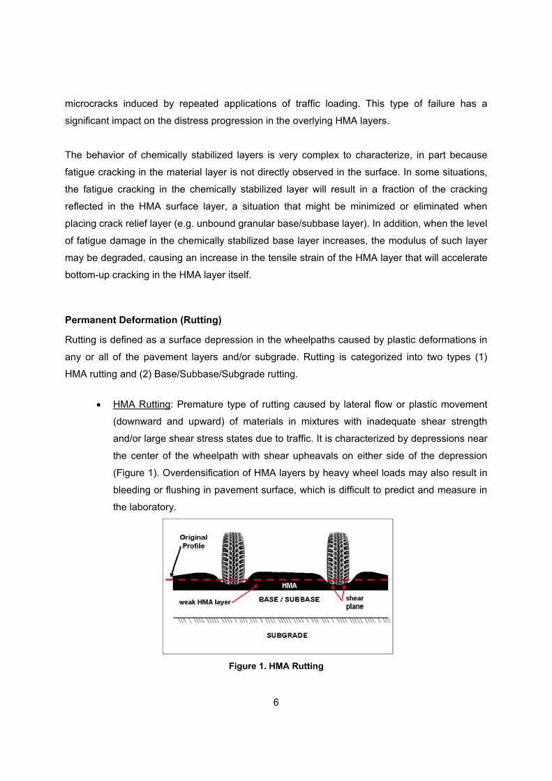
Permanent Deformation (Rutting)
Rutting is defined as a surface depression in the wheelpaths caused by plastic deformations in
any or all of the pavement layers and/or subgrade. Rutting is categorized into two types (1)
HMA rutting and (2) Base/Subbase/Subgrade rutting.
• HMA Rutting: Premature type of rutting caused by lateral flow or plastic movement
(downward and upward) of materials in mixtures with inadequate shear strength
and/or large shear stress states due to traffic. It is characterized by depressions near
the center of the wheelpath with shear upheavals on either side of the depression
(Figure 1). Overdensification of HMA layers by heavy wheel loads may also result in
bleeding or flushing in pavement surface, which is difficult to predict and measure in
the laboratory.
Figure 1. HMA Rutting

7
• Base/Subbase/Subgrade Rutting: Vertical compression caused by material
densification due to excessive air voids or inadequate compaction of any of the
bound or unbound pavement layers when subjected to traffic loads. It manifests as
depressions near the center of the wheelpath without a hump on either side of the
depression (Figure 2). The severity of the depressions caused by secondary rutting
varies from low to moderate.
Figure 2. Base/Subbase/Subgrade Rutting
Permanent deformation is the cumulative sum of ruts occurring in all layers of the pavement
system. No permanent deformation is assumed to occur for chemically stabilized materials,
PCC (Portland Cement Concrete) fractured slab materials and bedrock; they are assumed to
have no contribution to the total permanent deformation of the pavement system.
2.3. Destructive Structural Evaluation
Destructive testing techniques involve evaluating a specimen (pavement structure in this case)
by changing its original shape or properties. The most common destructive evaluation
technique in pavements is physical removal of pavement layer material by coring. Samples are
usually 10 or 15 centimeters in diameter (Figure 3) and are used to identify layers of different
materials and their thicknesses, and to examine general material condition. The observation of
samples can supplement the information obtained from visual distress surveys and helps
identifying the potential causes of structural problems (e.g. lack of bonding between layers,
stripping of AC layers, and presence of defects such as cracks or voids). Laboratory tests are
commonly used to characterize materials, i.e., determine material mechanical properties such
as strength and modulus of different layers. Destructive testing has the advantage of allowing

8
the observation of subsurface conditions of pavement layers and bonding within them, which
usually cannot be obtained with other methods.
Figure 3. Core Sample
Coring and boring require a considerable amount of samples and tests to characterize the
different materials that compose the pavement’s structure. Thus, some limitations of this type of
procedure include its intrusive nature and the disruption of trafficked areas (Figure 4), the
amount of time and labor required, and its cost. However, it is generally essential to perform a
destructive test program to complement NDT techniques.
Figure 4. Coring Machine and Core Extraction
2.4. Nondestructive Structural Evaluation
Nondestructive testing (NDT) involves the assessment of pavement structure and material
properties by utilizing methods that will not change the structure’s properties or induce damage
into it. There are several available NDT techniques for use in pavement structural evaluation;

9
some of the most common types include visual surveys, Ground Penetrating Radar (GPR), and
deflection testing (FWD). These types of technologies offer advantages like the reduction of
costs, reduction of occurrence of accidents due to lane closures, faster data collection, and
greater area coverage. NDT results can provide a reliable evaluation of in situ structural
adequacy, which is needed for the selection and design of rehabilitation treatments.
The selection of NDT technologies for pavement evaluation depends on the existing budget,
speed, productivity, and required quality of collected data. The NDT technologies utilized in this
investigation are the following:
(1) Visual survey: Observation, measurement and mapping of pavement distresses.
(2) Ground Penetrating Radar (GPR): Determination of layer thickness and irregularities.
(3) Falling Weight Deflectometer (FWD): Determination of in situ pavement structural
properties.
2.4.1. Visual Survey
Visual survey can vary from a windshield survey carried out from a moving vehicle to a detailed
survey performed by walking the project to measure and map out the identified distresses on
the pavement (including surface, shoulders, and drainage systems). The survey technique
adopted for this research is based on a video of the surface taken by a high-speed, downward
looking digital video camera.
The raw data collected during the survey must be processed for the pavement evaluation and
analysis. Several methods are available to measure and quantify distresses and they vary from
agency to agency. It is important that the quantification of the distresses (e.g. area of alligator
cracking and length of longitudinal cracking at each severity level) is compatible with the
distress rating tables to be used.
The identification of significant load-related surface distresses in the visual condition survey
could be an indication that the pavement is approaching or has already reached the end of its
service life. Examples of load related distresses for flexible pavements include fatigue cracking
and rutting. The structural adequacy can be determined by comparing the severity and extent of
load related distresses to specific thresholds, which depend on highway classification. An
10
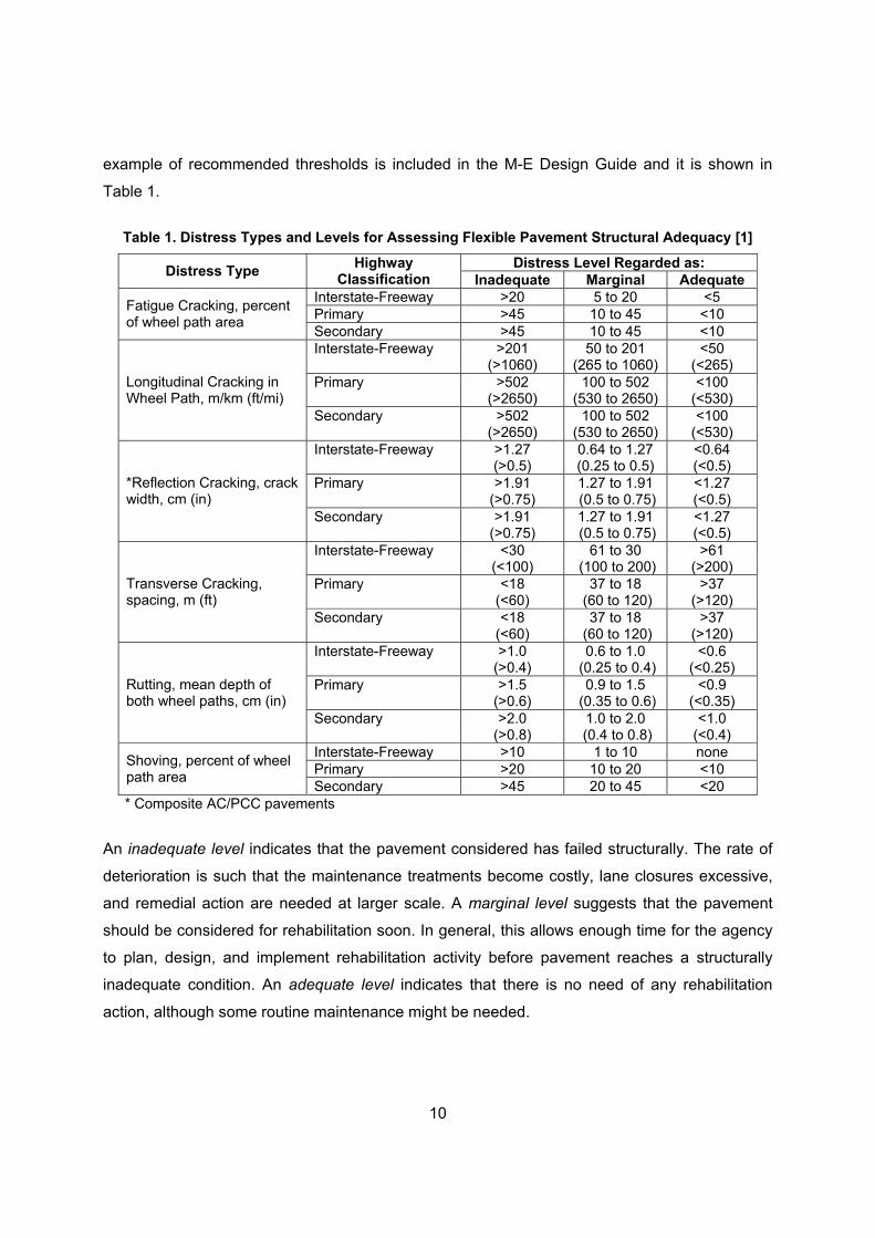
example of recommended thresholds is included in the M-E Design Guide and it is shown in
Table 1.
Table 1. Distress Types and Levels for Assessing Flexible Pavement Structural Adequacy [1]
Distress Level Regarded as: Distress Type Highway Classification Inadequate Marginal Adequate
Interstate-Freeway >20 5 to 20 <5 Primary >45 10 to 45 <10 Fatigue Cracking, percent
of wheel path area Secondary >45 10 to 45 <10 Interstate-Freeway >201
(>1060) 50 to 201
(265 to 1060) <50
(<265) Primary >502
(>2650) 100 to 502
(530 to 2650) <100
(<530) Longitudinal Cracking in Wheel Path, m/km (ft/mi)
Secondary >502 (>2650)
100 to 502 (530 to 2650)
<100 (<530)
Interstate-Freeway >1.27 (>0.5)
0.64 to 1.27 (0.25 to 0.5)
<0.64 (<0.5)
Primary >1.91 (>0.75)
1.27 to 1.91 (0.5 to 0.75)
<1.27 (<0.5)
*Reflection Cracking, crack width, cm (in)
Secondary >1.91 (>0.75)
1.27 to 1.91 (0.5 to 0.75)
<1.27 (<0.5)
Interstate-Freeway <30 (<100)
61 to 30 (100 to 200)
>61 (>200)
Primary <18 (<60)
37 to 18 (60 to 120)
>37 (>120)
Transverse Cracking, spacing, m (ft)
Secondary <18 (<60)
37 to 18 (60 to 120)
>37 (>120)
Interstate-Freeway >1.0 (>0.4)
0.6 to 1.0 (0.25 to 0.4)
<0.6 (<0.25)
Primary >1.5 (>0.6)
0.9 to 1.5 (0.35 to 0.6)
<0.9 (<0.35)
Rutting, mean depth of both wheel paths, cm (in)
Secondary >2.0 (>0.8)
1.0 to 2.0 (0.4 to 0.8)
<1.0 (<0.4)
Interstate-Freeway >10 1 to 10 none Primary >20 10 to 20 <10 Shoving, percent of wheel
path area Secondary >45 20 to 45 <20 * Composite AC/PCC pavements
An inadequate level indicates that the pavement considered has failed structurally. The rate of
deterioration is such that the maintenance treatments become costly, lane closures excessive,
and remedial action are needed at larger scale. A marginal level suggests that the pavement
should be considered for rehabilitation soon. In general, this allows enough time for the agency
to plan, design, and implement rehabilitation activity before pavement reaches a structurally
inadequate condition. An adequate level indicates that there is no need of any rehabilitation
action, although some routine maintenance might be needed.

11
2.4.2. Ground Penetrating Radar (GPR)
The determination of the thicknesses of the layers that compose the pavement structure can be
performed using a Ground Penetrating Radar (GPR). Layer thicknesses are determined by
sending pulses of electromagnetic energy with a radar system and detecting the electrical echo
produced when the pulse encounters electromagnetic discontinuities (e.g., sudden variations in
material properties, existing pipes, and voids). Figure 5 illustrates a pavement structure
subjected to GPR testing. An image of the profile of the layers inside the pavement system can
be generated by the reflected waves that are received by the radar moving across the surface of
the pavement. The result is a profile of the elapsed time between the penetration of the
electromagnetic pulse into the pavement system and the back bounce to the GPR receiver. The
longer period of time it takes to obtain the returning signal, the further the signal would have
traveled. The true depth of layers is determined by converting this time profile into thicknesses.
Figure 5. Pavement Structure Subjected to GPR Testing
Interpreting GPR data and profiles is not a simple task because interpretations are usually
ambiguous. Few are the measurements that have such quality data that can be literally
interpreted. Sometimes the analysis works better by interpolating between known values, e.g.,
thickness measurements between cores at different locations or extrapolations from known
pavement profiles. One of the limitations in differentiating pavement layers is when the
materials have similar dielectric properties, creating a difficult scenario for a type of radar that
depends on the electromagnetic contrast to distinguish between material, occasionally making
these interfaces invisibles.
HMA
BASE
SUBGRADE
GPR antenna
HMA
BASE
SUBGRADE
GPR antenna

12
2.4.3. Deflection Testing – Falling Weight Deflectometer (FWD)
The magnitude and shape of the pavement’s surface deflection when subjected to loading
reflects its structural condition and can also be used to determine the load transfer efficiency for
rigid pavements. Deflection testing is a common type of pavement NDT method used to
quantify the variability of pavement strength within a project, evaluate the structural adequacy of
the pavement, determine the in situ modulus of each of the pavement layers, and determine
remaining service life by characterizing the pavement response to loading for flexible (asphalt)
pavements [12]. For rigid pavements, FWD tests are used to determine the concrete elastic
modulus and subgrade modulus of reaction (at the slab center), void detection, and load
transfer efficiency of cracks and joints. The layer properties are calculated by using static load
analytical procedures and empirical performance relationships applied to the dynamic deflection
data [13].
Different types of deflection testing equipment are commercially available. However, Falling
Weight Deflectometer (FWD) (Figure 6) is the most frequently used device to evaluate
pavements because it is the one that better simulates the load from a moving tire in both
magnitude and duration [8]. These devices measure the pavement surface deflection caused
by a dropping load using velocity transducers (seismometers, geophones).
Figure 6. FWD – Dynatest Model 8002
Falling weight deflectometers deliver a transient force impulse to the pavement surface. A brief
description of the operation sequence is as follows:
• A weight is hydraulically lifted to a given height on a guide system and is then
dropped to simulate the deformations produced by a moving tire (Figure 7).

13
Figure 7. Deformations of Pavement Subjected to Loading
• The force of the falling weight is transmitted to the pavement through a circular foot
plate with a diameter of 30 cm (11.8 in) (a 45 cm (17.7 in) plate can be also used
when testing directly over unbound layers).
• The surface deflection caused by the impulse load is measured by deflection sensors
(geophones). Usually seven to nine geophones are used; the first one mounted in
the center of the loading plate and the rest positioned at various distances from it (up
to 2.5m (98in) from the center of the loading plate). The loading plate and geophones
are shown in Figure 8.
• Peak deflection values are recorded to be stored and displayed.
Figure 8. Loading Plate and Geophones
The applied impulse load (with duration from 20 ms to 60 ms depending on the equipment
manufacturer) may be varied between 11 kN (2.5 kips) to 120 kN (27.0 kip) by modifying the

14
mass, the drop height, or both. However, it is recommended that the FWD load should be in the
range of 40 kN (9.0 kips) to 53.4 kN (12 kips) so that the layer moduli predictions will be
representative of pavement response under heavy truck wheel loads. The FWD load level used
for testing AC and PCC pavements may affect the backcalculated moduli obtained from the
deflection data, particularly for non-linear unbound granular and subgrade materials.
2.4.4. Moduli Backcalculation
The procedure used to estimate the in situ elastic moduli for each pavement layer (including the
subgrade) based on the measured deflections is called backcalculation. The backcalculation
procedure involves calculating theoretical deflections under the applied load using assumed
pavement layer moduli. These theoretical deflections are then adjusted in an iterative process
until the theoretical and measured deflections reach an acceptable agreement (low Root Mean
Square error - RMS) and reasonable backcalculated moduli for each layer are obtained. The
RMS error is defined as the absolute difference between the measured and computed deflection
basins expressed usually as percentage.
Several backcalculation algorithms and software are commercially available. Even though
many of the software packages may have some similarities, the results can differ depending on
assumptions, iteration technique, and backcalculation or forward calculation schemes used
within the programs. Some examples include ELMOD, EVERCALC, ILLI-BACK, MODCOMP5,
MODULUS, and WESDEF.
Typical Moduli Values
Backcalculated results are usually compared to typical stiffness moduli for each material, such
as the ones presented in Table 2. Some of the presented values were obtained from the
available literature [4], [7], [18] and others were estimated from experience. Ranges are usually
specified for all materials in order to improve the reasonableness of the results.
Since the deflection testing program is performed at a particular month or season of the year,
the backcalculated values are representative of only that period of the year. Correction factors
should be taken into account for the seasonal changes; the best practice to obtain these factors
is by performing deflection measurements at different times of the year.

15
Table 2. Typical Stiffness Moduli for Different Materials
Range of values, MPa (ksi) Material
Initial Modulus, MPa
(ksi) Low High Asphalt Materials Hot Mix Asphalt 3,500 (500) 2,000 (300) 5,500 (800) PCC Materials Intact slab 31,000 (4,500) 20,500 (3,000) 41,500 (600) Fractured slab 3,500 (500) 700 (100) 20,500 (3,000) Open Grade Drainage Layers Asphalt Stabilized 1,000 (150) 700 (100) 1,700 (250) Cement Stabilized 1,700 (250) 1,000 (150) 2,400 (350) Cement Stabilized Layers 21A 5,800 (850) 4,800 (700) 13,800 (2,000) Cement Treated Aggregate 5,800 (850) 4,800 (700) 13,800 (2,000) Stabilized Subgrade 2,400 (350) 900 (130) 3,800 (550) Unbound Materials Crushed stone/gravel, Base 350 (50) 70 (10) 1,000 (150) Gravel or soil-agg. mix, coarse Base 200 (30) 70 (10) 700 (100) Gravel or soil-agg. mix, fine Base 150 (20) 35 (5) 550 (80)
Spatial Frequency
Another important issue when performing FWD tests is the spacing between consecutive
measurements. This spatial frequency depends on the length of the road section under
investigation and level of investigation (network or project level). The spacing may vary from 50
m (165 ft) to 100 m (330 ft) for project level investigations, and between 200 m (660 ft) to 250 m
(820 ft) for network level. Higher frequencies are used for research purposes. Testing may be
performed in the outer wheelpath (area subjected to traffic loading) or in the center of the lane
(for comparison with wheelpath results). Figure 9 shows a schematic of the stress zone of a
pavement under FWD testing.
Figure 9. Stress Zone of a Pavement Subjected to FWD Testing

16
2.5. M-E Design Analysis for Flexible Pavements
The Mechanistic-Empirical (M-E) design presented in this section is applicable for new and
reconstructed flexible pavements. For the purpose of this study, flexible pavements are defined
as structures having asphalt concrete surfaces. The analysis is an iterative procedure where a
trial design is analyzed to determine if it meets the established performance criteria, including:
permanent deformation (rutting), fatigue cracking (bottom-up and top-down), chemically
stabilized layer fatigue fracture (only for composite pavements), thermal cracking, and
smoothness (International Roughness Index or IRI). Table 3 is a summary of the flexible
pavements design process steps.
Table 3. Design Process Steps
# Step Description
1 Trial design for specific site conditions
Define subgrade, asphalt concrete and other paving material properties, traffic loads, climate, pavement type, and design and construction features
2 Acceptable pavement performance criteria
Establish acceptable levels of rutting, fatigue cracking, thermal cracking, and IRI at the end of the design period
3 Reliability level for each performance measure
Select desired level of reliability level for, rutting, cracking, IRI. Reliability is defined as the probability that a component or system will satisfactorily perform its specified function for the specified or required period of time under given or predicted operating conditions [13]
4 Input needed information to obtain monthly values of site conditions
Input needed information to obtain material’s seasonal variation, and monthly changes in traffic and environment for the entire design period
5 Compute structural responses (stresses and strains)
Use multilayer elastic theory or finite element-based pavement response models for each axle type and load and for each damage-calculation increment throughout the design period
6 Calculate distress/damage Calculate accumulated distress/damage at the end of each analysis period for the entire design period
7 Predict key distresses Use M-E Guide performance models to predict distresses at the end of each analysis period throughout the design life
8 Predict smoothness (IRI) Predict smoothness as function of: initial IRI, accumulated distresses over time, and site factors at the end of each analysis increment
9 Evaluate expected performance
Evaluate the expected trial design performance at the given reliability level.
10 Modify design Modify design if performance criteria is not met
2.5.1. Design Inputs
The required inputs for the trial design include project site conditions, such as subgrade and
material properties, presence of bedrock, traffic information and climatic data. In addition, there
are design inputs related to construction, such as initial smoothness (in terms of International

17
Roughness Index or IRI), estimated month of construction, and estimated month that the
pavement will be opened to traffic.
There are three input levels in the M-E analysis process; the input level must be selected based
on the importance of the project, available information/resources, and available time. A
description of the input levels is presented in Table 4.
Table 4. Description of Design Input Levels
Level Description Examples
1 Direct testing or measurements to obtain site and/or material inputs
- Material properties obtained through laboratory testing - Measured traffic volumes and weights at the project
site
2 Determine required inputs by the application of correlations
- Estimation of unbound base or subgrade resilient modulus from CBR or R-values using empirical correlations
3 Define inputs by utilizing national or regional default values
- Determination of typical resilient modulus value from AASHTO soil classification
- Determination of normalized axle weight and truck type distributions from roadway type and truck type classification
It is important to mention that it is not required that the input levels for all the parameters be the
same, i.e., asphalt concrete can be obtained from laboratory testing (Level 1) and climatic
information from regional data (Level 3).
The input data for new flexible pavement design is divided in six categories: (1) General
information; (2) Site/project identification; (3) Analysis parameters; (4) Traffic; (5) Climate, and
(6) Pavement structure. The information required within each category is explained as follows:
1. General Information: Expected design life (years), estimated month in which the base
and subgrade are going to be constructed, pavement (HMA) construction month
(defines time t = 0 for the HMA material aging model and thermal cracking model),
expected traffic opening month, and pavement type.
2. Site/project identification: Project location and identification, pavement’s functional
class (principal arterial, minor arterial, major collector, minor collector, local routes,
and streets).
3. Analysis parameters: Selection of some or all of the performance indicators (fatigue
cracking, thermal cracking, permanent deformation and pavement smoothness) and

18
establishment of criteria to evaluate a design. The magnitude of allowable distresses
(thresholds) recommended by the M-E Design Guide are included in Table 5.
Table 5. Allowable Distress Limits Recommended by the M-E Design Guide
Distress Type Allowable Value Surface-down (longitudinal cracking) 190m/km (1,000ft/mi) Bottom-up (fatigue cracking) 25% to 50% of total lane area Thermal cracking 190m/km (1,000ft/mi) Fatigue fracture of CSL* Damage index < 25% Total permanent deformation 75mm to 125mm (0.3in to 0.5in) Terminal Smoothness (IRI) 2.35m/km to 3.95m/km (150 to 250in/mile)
*CSL = Chemically Stabilized Layers
4. Traffic: The load spectra for single, tandem, tridem, and quad axles is specified
utilizing the following traffic information:
• Basic information: Annual Average Daily Truck Traffic (AADTT), percentage
of trucks in the design direction (directional distribution factor), percentage of
trucks in the design lane (lane distribution factor), and vehicles operational
speed (used in the asphalt bound layers moduli calculation).
• Traffic Volume Adjustment: Monthly adjustment factors, vehicle class
distribution (classes 4 through 13), hourly truck-traffic distribution, and traffic
growth factors.
• Axle Load Distribution Factors: Percentage of the total axle applications
within each load interval for a specific axle type and vehicle class (classes 4
through 13). Data provided for each month for each vehicle class.
• General Traffic Inputs: Mean wheel location, traffic wander standard
deviation, design lane width, number of axle types per truck class, axle
configuration, and wheelbase.
5. Climate: The weather related factors (required as hourly averages over the design
period) are: air temperature, precipitation, wind speed, percentage sunshine, and
ambient relative humidity. Seasonal or constant water table depth at the project site
is also considered.
6. Pavement Structure:
• Drainage and surface characteristics: Pavement surface layer absorptivity,
infiltration potential, cross slope, and length of drainage path.
• Layer properties:

19
Asphalt Concrete and Asphalt Stabilized Layers: Layer thickness,
Poisson’s ratio, thermal conductivity, heat capacity, total unit weight.
Laboratory-measured dynamic modulus (Level 1 input), mix properties
(Level 2 and 3 inputs), Superpave or conventional laboratory binder
test data (Level 1 input), specific PG grade, Viscosity Grade or
Penetration Grade (Level 2 and 3 input), dynamic modulus from FWD
backcalculation and/or predictive equations (Level 2 and 3 input),
volumetric effective binder content, air voids, reference temperature
for master curve development, average tensile strength at 14°F, creep
compliance data, and mix coefficient of thermal contraction.
Chemically Stabilized Layers: Maximum design resilient modulus,
minimum resilient modulus (after fatigue damage), modulus of rupture,
unit weight, Poisson’s ratio, thermal conductivity, and heat capacity.
Unbound Base/Subbase/Subgrade: Layer thickness, resilient modulus
(Level 1: using nonlinear finite element code; Level 2: directly
specified from FWD backcalculation or empirical relations; Level 3:
specified default resilient modulus as a function of AASHTO or Unified
Soil Classification), Poisson’s ratio, and coefficient of lateral earth
pressure (K0).
Bedrock: Presence of bedrock within 3 m (10 ft) of the pavement
surface influences the structural response of pavement layers; inputs
for this layer include: layer thickness, unit weight, Poisson’s ratio, and
layer modulus.
• Distress potential: These are supplementary properties required for
smoothness (IRI) prediction models. The prediction of the development of
additional distresses affecting smoothness are used with empirical relations
that are not mechanistically considered by the M-E Guide, e.g., block
cracking and sealed longitudinal cracks outside the wheelpath.
2.5.2. Critical Response Variables and Pavement Response Models
There are different critical variables that determine the pavement structural response to traffic
loads and environmental influences. Environmental factors may influence the structure directly
(e.g., strains due to thermal expansion and/or contraction) or indirectly through effect of material
properties (e.g., changes in stiffness due to temperature and/or moisture effects).

20
The pavement response models were developed to determine the critical response variables
that affect the development of specific distresses. The output of the pavement response models
are stresses, strains, and displacements within the pavement layers. These outputs can be
used in pavement distress prediction models (also called transfer functions), which will
determine the structure’s performance. Examples of pavement distresses that can be predicted
utilizing these critical variables include the following:
- HMA fatigue cracking: Tensile horizontal strain at the bottom/top of HMA layer.
- HMA rutting: Compressive vertical stresses/strains within the HMA layer.
- Unbound layers rutting: Compressive vertical stresses/strains within the base/subbase
layers.
- Subgrade rutting: Compressive vertical stresses/strains at the top of the subgrade.
2.5.3. Incremental Distress and Trial Design Suitability
Critical stresses and/or strains for each distress type are estimated for an increment or design
analysis period. An increment is defined as a shorter analysis period in which the target design
life is divided into, starting with the traffic opening month. The basic unit for estimating the
damage is one month, however, modulus values may vary rapidly during freeze and thaw
conditions; therefore the analysis interval is reduced to two-week periods. These critical stress
and/or strain values are converted to incremental distresses in absolute terms (e.g., incremental
rut depth) or in terms of damage index (e.g., fatigue cracking). The suitability of the trial design
is analyzed by summing all increments of distresses and/or damage at the end of each analysis
period; this procedure is performed automatically by the M-E Design Software.
21
Chapter 3 - RESEARCH APPROACH
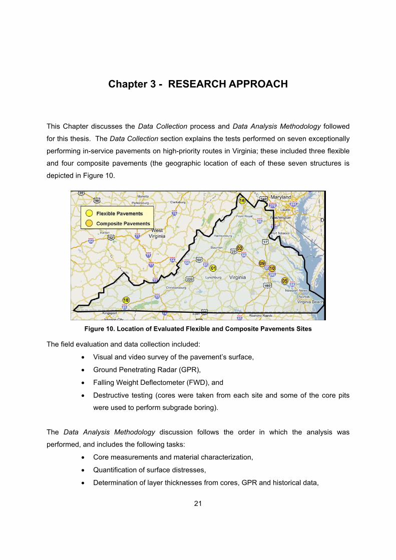
This Chapter discusses the Data Collection process and Data Analysis Methodology followed
for this thesis. The Data Collection section explains the tests performed on seven exceptionally
performing in-service pavements on high-priority routes in Virginia; these included three flexible
and four composite pavements (the geographic location of each of these seven structures is
depicted in Figure 10.
Figure 10. Location of Evaluated Flexible and Composite Pavements Sites
The field evaluation and data collection included:
• Visual and video survey of the pavement’s surface,
• Ground Penetrating Radar (GPR),
• Falling Weight Deflectometer (FWD), and
• Destructive testing (cores were taken from each site and some of the core pits
were used to perform subgrade boring).
The Data Analysis Methodology discussion follows the order in which the analysis was
performed, and includes the following tasks:
• Core measurements and material characterization,
• Quantification of surface distresses,
• Determination of layer thicknesses from cores, GPR and historical data,

22
• Deflection analysis, backcalculation and comparison with laboratory results,
• Determination of the effective (current) structural capacity for flexible and
composite pavements using the 1993 AASHTO Design Methodology (in terms of
structural number (SN) and equivalent slab thickness (D), respectively), and
• Performance prediction of the selected structures and comparison of the
predicted pavement damage with the actual pavement distresses
observed/measured in the field.
The following sections describe the methodology used in each of these tasks.
3.1. Data Collection
Given that the evaluated sections were located mainly on interstate and other high-traffic routes,
the sections lengths were set at 0.8 km (0.5 mi) to avoid excessive delays to the public during
field evaluation; Table 6 shows a summary of the selected test sections and their locations.
Table 6. Selected Pavement Sites
Site # County Route Direction Milepost Pavement
Age/Surface Age (yrs)
FLEXIBLE PAVEMENTS 01 Amherst 29 South 7.80-7.30 34 / 11 16 Frederick 81 North 21.31-21.87 39 / 13 18 Washington 81 South 1.50-1.00 5 / 3
COMPOSITE PAVEMENTS (CRCP Rehab.) 02 Albemarle 64 East 12.99-13.37 34 / 12 05 New Kent 64 East 14.69-15.19 32 / 13 09 Henrico 295 South 5.29-5.79 23 / 6 10 Hanover 295 South 9.52-10.02 24 / 9
3.1.1. GPR Testing
Ground penetrating radar was used in this project to determine the layer thicknesses of the
selected pavement. The GPR system used was a SIR-10B control unit, manufactured by
Geophysical Survey Systems, Inc. (GSSI), and connected to a 1GHz air-coupled and/or a 1.5
GHz ground-coupled antenna. All GPR surveys were conducted using the test van showed in
Figure 11. The van has an antenna fixture in the back that allows deployment of the GPR
antennas at three different transverse locations (right wheel path, center, and left wheel path).

23
One or two antennas were used depending on the surveyed pavement structure. The selection
of the suitable antennas and of the GPR acquisition rate for each project was based on the
following criteria:
1. For the flexible sections, GPR data was collected using the air-coupled antenna at a
speed ranging between 48 km/h (30 mi/h) and 65 km/h (40 mi/h).
2. For the composite sections incorporating reinforcement, GPR data was collected
simultaneously by the air-coupled and the ground-coupled antennas. The test speed
was limited by the ground-coupled antenna to 8 km/h (5 mi/h).
Figure 11. Antenna Used for GPR Collection
In addition, stationary GPR measurements (i.e., data collected while the GPR van was stopped)
were taken near the core locations before extraction of the cores. This was done to validate the
GPR thickness measurements and estimate their accuracy.
3.1.2. Visual/Video Survey
A visual survey of the pavement surface condition was performed based on a video taken by a
high-speed, downward looking digital video camera. As showed in Figure 12, the digital camera
used to collect the video was mounted on the GPR van. The visual survey was synchronized
with the same DMI (Distance Measurement Instrumentation) used to control the GPR data
acquisition.

24
Figure 12. Digital Camera Used for Video Survey
3.1.3. FWD Testing
Falling Weight Deflectometer (FWD) measurements were performed to determine the structural
condition of each of the test sites evaluated for the Premium Pavement Project. All tests were
conducted using the Virginia Department of Transportation (VDOT) Dynatest model 8002 FWD
unit (Figure 13). The three main components of this system include: (1) Dynatest 8002-054
FWD Trailer; (2) Dynatest 9000 system Processor and (3) Laptop computer. The peak
deflections caused by the applied load were registered by nine sensing transducers
(geophones). Sensor located at 0, 203, 305, 457, 610, 914, 1219, 1524 and 1829 mm (0, 8, 12,
18, 24, 36, 48, 60 and 72 in) from the center of the loading plate were used.
Figure 13. FWD Used by VDOT

25
Fourteen drops were applied at each FWD testing point, including two seating drops of 40kN
(9,000lbs), and three drops at each of the following load levels: 26.7kN (6,000lbs), 40kN (9,000
lbs), 53.4kN (12,000lbs) and 71.2kN (16,000lbs) respectively. The test frequency and location
varied for each pavement type; but in general the frequencies used were the following:
(1) Flexible pavement tests every 15.24m (50ft) on the right wheelpath.
(2) Composite pavement tests every 15.24m (50ft) on the center of the lane (between
wheelpaths).
Temperature data were collected during all FWD tests. Both the surface and air temperatures
were measured using Raytek and Dynatest sensors, respectively.
3.1.4. Coring/Boring
The coring activities were customized to the material being sampled. For flexible material
sampling, 150mm (6in) cores were taken through at least the thickness of the bound asphalt
layers. The 150mm size was necessary for anticipated testing of the larger-stone base
mixtures. Ten cores were extracted from each full-depth asphalt section at a distance of
approximately 60m (200ft) alternating between the right wheelpath and the lane center.
Sampling of composite pavements was modified based on site conditions and specific
pavement composition. For composite sections that contained no larger-stone asphalt base
mixes, partial depth sampling for bound asphalt and full-depth sampling for concrete was done
with the 100mm (4in) barrel. If the asphalt materials include a larger-stone base mix, at least
some portion (generally partial depth) of the sampling was done using the 150mm barrel.
Generally, at least 6-cores spaced at 90m (300ft) intervals were taken from every test section.
In addition to the coring of the bound layers of the pavement, soil sampling and testing were
also conducted at each test section. The local district geology crew conducted the soil
investigation activities. Soil boring was confined to two core-holes per test site. Continuous
0.45m (1.5ft) split-spoon sampling was conducted to approximately 1.35m (4.5ft) below the
bottom of the bound material. All soil boring activities were completed according to established
VDOT procedures and field adaptations of ASTM standard D1586. All soil descriptions were
made in accordance with ASTM D2488.

26
3.2. Data Analysis Methodology
The methods used to analyze the data collected from the visual survey, GPR, FWD testing and
coring and boring are discussed in this section as well as the purpose of including them in this
research. The backcalculation procedure, the use of the M-E Design Software to predict
pavement performance using input parameters obtained from the NDT evaluation (such as
backcalculated moduli), and the transfer functions that the software utilizes to quantify and
predict pavement damage are also considered in this section.
3.2.1. Visual Distress Quantification
The digital videos were used to obtain the current pavement distresses based on the Distress
Rating Manual used by VDOT [21], [22]. The process involved analyzing the videos and
manually quantifying the identified distresses with the purpose of determining the adequacy
level of the structures, defined as: inadequate, marginal or adequate (see Section 2.4.1. )
3.2.2. Core Measurements and Material Characterization
The different layers observed on each of the obtained cores were visually evaluated to identify
problems and measured to check the accuracy of the GPR results and to compare to historical
data. In addition, some cores were used for material characterization.
Laboratory tests were performed to selected asphalt and concrete samples obtained from the
coring procedure. Three 150-mm cores from each section were used to determine the resilient
modulus of the asphalt in accordance to ASTM D4123. Each core provided one sample from the
wearing surface and one sample from the base mix. Tests were run for 100 cycles and the last
five were used to calculate the resilient modulus. The durations of the pulse load and rest
period were 0.1 and 0.9 sec respectively. The applied load was chosen to induce deformations
that are well above the sensitivity of the strain gauges without damaging the specimens. The
applied loads were determined as 1000 N (225 lb) and 2000 N (450 lb) for the wearing surface
and BM layers respectively. All tests were performed at 25oC (77oF). Specimens were stored in
the laboratory at room temperature (25oC). Before being tested, specimens were placed in an
environmental chamber at 25oC (77oF) for a period of 1 hour.
27
The concrete cores were subjected to compressive strength (f’c) tests in accordance to ASTM
C39/C39M-99. The elastic modulus of the concrete was determined utilizing the equation
recommended by the American Concrete Institute (ACI):
Ec = 57,000 (f’c)1/2 (1)
where,
Ec = elastic modulus of the concrete (psi), and
f’c = compressive strength of the concrete (psi).
Two cores were tested per site and they were cut to a height of 203 mm (8 in) prior to testing. A
Forney compression machine was used to perform all the tests.
3.2.3. Layer Thickness Determination
Three sources of information were compared in order to obtain accurate information about the
thicknesses of the different layer materials within each of the pavement structures: measured
cores, GPR results and historical data. The measured cores were considered to be the most
reliable source of information but unfortunately the cores were not obtained for the whole depth
of the structures. In situations where the thickness of the layers could not be determined by
measured cores, GPR thicknesses were utilized, followed by historical data when GPR results
could not detect certain interfaces.
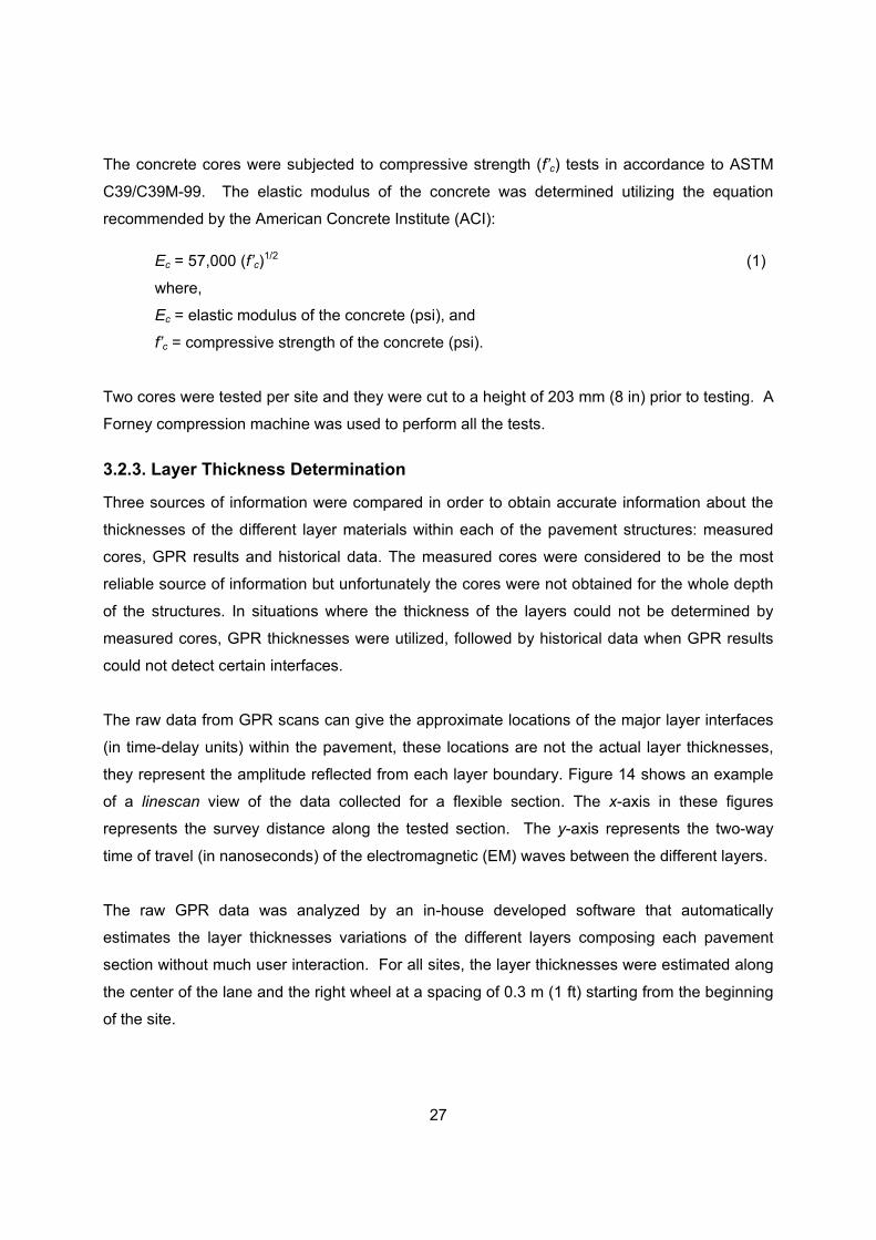
The raw data from GPR scans can give the approximate locations of the major layer interfaces
(in time-delay units) within the pavement, these locations are not the actual layer thicknesses,
they represent the amplitude reflected from each layer boundary. Figure 14 shows an example
of a linescan view of the data collected for a flexible section. The x-axis in these figures
represents the survey distance along the tested section. The y-axis represents the two-way
time of travel (in nanoseconds) of the electromagnetic (EM) waves between the different layers.
The raw GPR data was analyzed by an in-house developed software that automatically
estimates the layer thicknesses variations of the different layers composing each pavement
section without much user interaction. For all sites, the layer thicknesses were estimated along
the center of the lane and the right wheel at a spacing of 0.3 m (1 ft) starting from the beginning
of the site.

28
Figure 14: Raw GPR Data, Center of the Lane, Flexible Section
The raw GPR data was analyzed by an in-house developed software that automatically
estimates the layer thicknesses variations of the different layers composing each pavement
section without much user interaction. For all sites, the layer thicknesses were estimated along
the center of the lane and the right wheel at a spacing of 0.3 m (1 ft) starting from the beginning
of the site.
It should be noted that depending on the pavement structure and the dielectric constant contrast
between materials of adjacent layers, some interfaces were not detected from the GPR data.
Examples of structures presenting this kind of problem include different types of thin HMA
layers; base layer and subgrade composed of materials having similar dielectric constants, and;
interface between concrete slab/base layer and other layers underneath the concrete.
An example of the layer thicknesses comparison between measured cores, GPR results, and
historical data is included in Table 7. It can be observed that even though the GPR radar
couldn’t distinguish between the HMA layers, the total HMA thickness is very similar to the
combined thickness for HMA layers measured from the cores and also the historical data. The
selection of thicknesses between historical data, GRP and cores for the rest of evaluated sites
is presented in Appendix A.
HMA
Base
Subgrade

29
Table 7. Selection of Thicknesses Between Historical Data, GPR and Cores for Site 16 (Flexible)
HISTORICAL DATA GPR CORES Layer
# Material Thickness (mm) Year Material Thickness
(mm) Material Thickness (mm)
1 SM-2C 46 1991 SM-2C 48.2 Surface Mix 39
2 I-3 10 1965
3 CB-1 or 33 -
4 H-3 191 -
I3 + CB1 + H3 233 Base Mix 256
5 Aggregate Base Type
1 152 - Aggregate
Base 125.4 - -
6 Select
Material Type 1
305 - - - - -
7 Subgrade - - Subgrade - Subgrade - NOTE: Shaded area indicates the thickness selected for each layer
3.2.4. Deflection Analysis
The in situ elastic moduli for all pavement layers were backcalculated from the measured
deflection at a 40 kN (9,000 lbs) load level. In addition, the variability of the deflections along
the section was investigated.
Deflection Variability Analysis
Given that pavement deflections vary with load magnitude, load plate characteristics and overall
pavement structure, it is recommended to express the variability in terms of the Coefficient of
Variation (CV) [1], which was computed using the following equation:
CV = (standard deviation / average) 100 (2)
Three levels of deflection variability were defined: Low (15%), Average (30%) and High (45%)
for D1 (center of the loading plate, it represents the deflections of the whole pavement
structure), D7 and D9 (common locations to measure the subgrade deflection).
Homogenous Sections
Each project was divided into homogeneous sections using the deflection data. The software
package called TAG (Total Analysis Group) was used to perform this task. TAG was developed
by VDOT to analyze FWD data and it was utilized in this project to obtain homogeneous

30
-0.070
-0.060
-0.050
-0.040
-0.030
-0.020
-0.010
0.0000 100 200 300 400 500 600 700
Distance (m)
Cum
ulat
ive
Sum
of D
efle
ctio
n - S
ite 0
2
Sensor 1 (0 mm from loading plate)
Sensor 7 (1219 mm from loading plate)
Selected Homogeneous Sections
sections for the pavement structures. Obtaining the cumulative sums of deflection allows
dividing each project into sections with similar performance [27]; as an example, Figure 15
illustrates the homogeneous sections obtained for Site 02. Two FWD sensors were selected to
obtain homogeneous sections: (a) Maximum deflection (sensor at 0 mm from loading plate
center), and (b) Sensor 7 (sensor at 1219 mm from loading plate center). Appendix B contains
the homogeneous sections for all the evaluated structures.
Layer Moduli Backcalculation
Many backcalculation programs are currently available; however, most of them are specially
designed to analyze flexible (asphalt) pavements, making it difficult to find a suitable
backcalculation program to evaluate composite and rigid pavements. The software package
used for the backcalculation process was ELMOD version 5.1, developed by Dynatest [5].
ELMOD’s approach is based on the Odemark-Boussinesq Method of Equivalent Thickness
(MET). ELMOD was selected as the backcalculation software because of its flexibility in the
data-input process, fast analysis, easiness in viewing results, and the ability to modify
parameters to analyze different case scenarios. These capabilities make it a practical software
package to use.
Figure 15. Homogeneous Sections Based on Cumulative Sum of Deflections – Site 2
3.2.5. Determination of Effective Structural Capacity
The structural capacity (or ability to carry loads) of the pavement changes with time and traffic.
When a structural evaluation is conducted on in-service pavements, the pavement’s structural
capacity is defined in terms of its effective structural capacity. For flexible pavements, the

31
structural capacity is measured by the structural number (SN); for rigid pavements, by the slab
thickness (D); and for composite pavements it is expressed as an equivalent slab thickness.
The various computations conducted for these estimations are presented in the following
sections.
Design (Original) Structural Number (SN)
The structural number of a pavement structure can be obtained by combining the structural
contribution from the each of the pavement layers, as follows [1]:
nnDaDaDaDaSN ++++= L331211 (3)
where,
Di = total thickness of all pavement layers above subgrade (in),
ai = layer coefficient, and
SN = structural number.
Effective Structural Number (SNeff) from Condition Survey
This method of determining the effective structural number of the AC pavements involves the
use of the same equation employed to calculate the Design Structural Number (SN), with the
difference of using suggested layer coefficients (ai’s) that depend on the type and amount of
present deterioration. Most of these suggested layer coefficients are less than the values
utilized for the same materials for new construction [1].
Effective Structural Number (SNeff) from NDT Evaluation
The effective structural number (SNeff) of a conventional flexible pavement can also be
determined from the NDT evaluation, assuming that the structural capacity of the pavement is a
function of its total thickness and overall stiffness [1]. Equation (3) shows the relationship
between SNeff, thickness and stiffness:
30045.0 peff EDSN ⋅=
(4)
where,
D = total thickness of all pavement layers above subgrade (in), and

32
Ep = effective modulus of pavement layers above the subgrade (psi).
Design Subgrade Resilient Modulus (Design MR)
The backcalculated subgrade resilient modulus can be used in the determination of the design
MR after applying an adjustment factor (C). This adjustment factor (C) is applied to make the
value calculated consistent with the value used to represent the AASHO Road Test subgrade; a
value of C of not greater than 1/3 is recommended, resulting in the following [1]:
Design MR = C * MR (5)
where,
Design MR = design subgrade resilient modulus (psi),
C = adjustment factor, 0.33 recommended, and
MR = backcalculated subgrade resilient modulus (psi).
Effective Modulus of the Pavement (Ep)
The effective modulus of the entire pavement structure (all pavement layers above the
subgrade) can be determined from the subgrade design resilient modulus, the total thickness of
all layers above the subgrade, and the maximum deflection (center of the load plate), applying
the following equation [1]:
+
−
+
+
⋅=p
R
pR
EaD
ME
aDM
apd
2
2
3
0
1
11
1
15.1
(6)
where,
d0 = deflection measured at the center of the load plate, adjusted to a standard
temperature of 68°F (in),
p = FWD load plate pressure (psi),
a = FWD load plate radius (in),
D = total thickness of pavement layers above subgrade (in),
MR = design subgrade resilient modulus (psi), and
Ep = effective modulus of all pavement layers above the subgrade (psi).

33
Effective Slab Thickness (Deff)
The effective slab thickness for composite pavements is determined from visual condition
survey, computed from the following equation:
( )
⋅
+⋅⋅= acac
durjcpcceff FD
FFDD0.2
(7)
where,
Deff = effective equivalent PCC thickness of existing AC/PCC (in),
Dpcc = thickness of existing PCC slab (in),
Dac = thickness of AC layer (in),
Fjc = joints and reflection cracks adjustment factor,
Fdur = durability adjustment factor (for “D” cracking and/or reactive aggregate), and
Fac = AC quality adjustment factor (distresses related to the AC layer which are not
eliminated by surface milling: rutting, stripping, shoving, weathering, and raveling).
3.2.6. M-E Design Guide Software Verification
The accumulation of damage as a function of time and traffic is the basis for the M-E design and
analysis of the trial pavement structure. The analysis for this thesis was performed using
version 0.701 of the M-E Design Guide software, which is available online. This software
package is an analysis that can predict pavement performance of new and/or rehabilitated
structures. The purpose of this study was to use the program to predict the performance of
selected structures (listed in Table 8) utilizing different layer properties obtained from the field
evaluation.
The historical data available for each structure was used to determine the date of construction
of the original pavement, the overlay year, and existing traffic (see Table 8). Two types of
analysis were performed, described as follows:
(1) New Pavement Design: The original structures were analyzed as new pavement designs from the construction year to the year of the application of the overlay, to
evaluate the predicted performance for the original structure. Unfortunately, there
were no historical records of the condition of the road before applying the overlay
to compare with the software’s output. The purpose of this analysis was to

34
estimate the condition of the pavement structure in the overlay year and to identify
the predicted critical distresses affecting each structure.
(2) Pavement Rehabilitation: This analysis was performed by using the rehabilitation design option from the overlay year to present time, and continued to the end of
the service life. The purpose of this analysis was to compare the current pavement
condition (established from the field evaluation performed in April and May 2004)
with the software’s output. This was used as a preliminary verification of the
distress prediction models applied to the investigated pavements. In addition, the
complete after overlay analysis (until failure) helped identifying the critical
distresses affecting each structure. Table 8. Summary of Pavement Structures Analyzed
Site # Layer Thickness,
mm (in) Original
Construction/Overlay(year/year)
Two-way AADTT
(year 2004) FLEXIBLE PAVEMENTS
SM + BM 240 (9.5) CTA 150 (6) 01 Subgrade -
1970 / 1993 2200
SM + BM 295 (11.5) Agg. Base + Select Material
430 (18) 16
Subgrade -
1965 / 1991 8560
SM + BM 375 (15) Asphalt OGDL 70 (3) Agg. Base 533 (21) 18
Subgrade -
1999 / 2001 11880
COMPOSITE PAVEMENTS SM + BM 115 (4.5) CRCP 209 (8.25) 02 Subgrade -
1970 / 1992 3360
SM + BM 108 (4.25) CRCP 203 (8) Agg. Base 150 (6) 05
Subgrade
1972 / 1991 1760
SM + BM 95 (3.75) CRCP 216 (8.5) CTA 150 (6) 09
Subgrade -
1980 / 1998 2000
SM + BM 100 (4) CRCP 200 (8) CTA 150 (6) 10
Subgrade -
1980 / 1996 6600
AADTT = Annual Average Daily Truck Traffic; SM = Surface Mix; BM = Base Mix; CTA = Cement Treated Aggregate; OGDL = Open Graded Drainage Layer; CRCP = Continuously Reinforced Concrete Pavement
35
The output of the analysis is automatically generated by the M-E Design software in Microsoft
Excel® spreadsheets. It includes a summary of the design inputs (general information, analysis
parameters, performance criteria, traffic, climate, and structure), and the predicted pavement
distresses accumulated in each increment or design analysis period (usually one month)
throughout the design life. The predicted pavement distresses are reported in both tabular and
graphic format. The remaining service life and the critical type of distresses can be estimated
from the damage accumulation charts for each distress.
Input Variables Table 9 presents a summary of sources of information for all the input parameters used to
predict pavement performance; these include historical data, field evaluation/analysis data,
State specifications, default and recommended values by the M-E Design Guide, and other
typical values.
Analysis Assumptions
The following assumptions were made in order to run the prediction performance analysis:
- The initial IRI after overlay was 1.0 m/km (63 in/mi) (default value recommended by
the M-E Design Guide).
- The allowable limits for all the types of distresses were the ones recommended by
the M-E Design Guide [10].
- Traffic will grow at a rate of 4% for all the evaluated sites during the design period.
- The vehicle class distribution for all the sites was Principal Arterials – Interstate and
Defense Routes, with a predominantly truck traffic (74%) of single trailer trucks, more
than 2% bus traffic, and less than 2% multi-trailer traffic [10].
- The properties of all the asphalt layers (asphalt mix gradation, volumetric properties,
and asphalt binder) are the ones specified to use in the Commonwealth of Virginia
[23], [24], [25], [26].
- The FWD backcalculated layer moduli for granular materials and subgrades are not
going to change significantly during the analysis period.
- The subgrade was approximately classified - using the Unified Soil Classification
System (USCS) - from the descriptions included in the boring field report.

36
Table 9. Input Parameters and Source of Information Input Parameter Source of Information
General Information Design life, existing pavement construction, pavement overlay construction, traffic open date
Historical data
Site/Project Identification Location, project ID, milepost from-to, traffic direction
Summary of selected test sites
Analysis Parameters (allowable limits) Initial IRI, Terminal IRI, longitudinal cracking (ft/mi), alligator cracking (%), AC thermal fracture (ft/mi), chemically stabilized layer fatigue fracture, AC rutting (in), total rutting (in)
Allowable distress values recommended by the M-E Design Guide
TRAFFIC Initial two-way AADTT, number of lanes per direction
Historical data
Percent of trucks in design direction, percent of trucks in design lane, operational speed (mph)
Default values for “Principal Arterials - Interstate and Defense Routes”
Traffic volume adjustment factors, monthly adjustments, vehicle class distribution, hourly distribution
Default values for Level 3 input
Traffic growth factor Historical data or typical values for the State of Virginia
Axle load distribution factors, number of axles per truck, axle configuration, wheelbase
Default values
CLIMATE Climatic data Climatic data from specific weather stations, and
interpolation of weather stations from VA, MD, NC, TN, KY, and WV. Zip files available at http://trb.org/mepdg/climatic_state.htm
STRUCTURE Asphalt Concrete: layer thickness Cores, GPR, and historical data Asphalt Concrete: asphalt mix gradation, grade, binder content, air voids
Historical data and State specifications [23], [24], [25], [26]
Asphalt Concrete: surface absorptivity, reference temperature, total unit weight (pcf), Poisson’s ratio, thermal properties
Default values for Level 3 input
CRCP and Chemically Stabilized Layers: layer thickness
Cores, GPR, and historical data
CRCP and Chemically Stabilized Layers: unit weight, Poisson’s ratio, thermal properties, mix properties
Historical data and State specifications
CRCP and Chemically Stabilized Layers: strength properties
Laboratory results and backcalculated modulus
Unbound Layers: layer thickness Cores, GPR, and historical data Unbound Layers: Poisson’s ratio, coefficient of lateral pressure, gradation, plasticity index
Default values and State specifications
Unbound Layers: Modulus Backcalculated modulus

37
Distress Models
The following structural distresses were considered: fatigue cracking (bottom-up and top-down),
fatigue cracking in chemically stabilized layers, and permanent deformation (rutting). This
section describes the failure mechanisms associated with these distresses and the transfer
functions that the software utilizes to quantify and predict pavement damage.
Fatigue Cracking: Bottom-up and top-down cracking models are based on the calculation of fatigue damage at the
bottom of each asphalt layer and at the surface, respectively. The estimation of fatigue cracking
damage is based upon Miner’s Law, where the damage is given by the following equation:
∑=
=T
1i i
i
NnD
(8)
where,
D = damage,
T = total number of periods,
ni = actual traffic for period i, and
Ni = traffic allowed under conditions prevailing in i.
The most common models used to predict the number of load repetitions to fatigue cracking (Ni)
are a function of the tensile strain and mix stiffness (modulus). The relationship used for fatigue
characterization in the M-E Design Guide is the following:
281.19492.3
111'00432.0
=
ECkN
tf ε
(9)
where,
Nf = number of repetitions to fatigue cracking,
k’1 = correction parameter for different asphalt layer thickness (hac) effects,
C = laboratory to field adjustment factor,
εt = tensile strain at the critical location, and
E = stiffness of the material.

38
a. Bottom-up cracking:
)49.302.11(
1
1003602.0000398.0
1'
ache
k−+
+=
(10)
b. Top-down cracking:
)8186.2676.15(
1
11201.0
1'
ache
k−+
+=
(11)
where,
hac = total thickness of the asphalt layers (in).
MC 10= (12)
−
+= 69.084.4
ba
b
VVV
M
(13)
where,
Vb = effective binder content (%), and
Va = air voids (%).
The final transfer function to calculate the fatigue cracking from the fatigue damage is
expressed as:
a. Bottom-up cracking (% of total lane area):
( )( )
+
= ⋅+ 601
16000
10010log'' 2211 DCCCCbottom eFC
(14)
where,
FCbottom = bottom-up fatigue cracking, percent lane area,
D = bottom-up fatigue damage,
C1 = 1.0,
C’1 = -2 * C’2,
C2 = 1.0, and
C’2 = -2.40874 – 39.748*(1 + hac)-2.856.
39
b. Top-down cracking (ft/mile):
( )( ) ( )56.101
100010010log5.30.7
+
= ⋅− Dtop eFC
(15)
where,
FCtop = top-down fatigue cracking (ft/mile), and
D = top-down fatigue damage.
Fatigue Fracture in Chemically Stabilized Layers: The relationship used in the M-E Design Guide to characterize the fatigue behavior of
chemically stabilized materials is defined in the following equation:
2
1
0825.0
972.0_log
c
tc MRDamageCTB
β
σβ
−
=
(16)
where,
CTB_Damage = number of repetitions to fatigue cracking of the CSM layer,
σt = maximum traffic induced tensile stress at the bottom of the CSM layer (psi),
MR = 28-day Modulus of Rupture (Flexural Strength) (psi), and
βc1 , βc2 = field calibration factors.
Due to the complexity of field selection design input and the difficulty of obtaining performance
data, the fatigue fracture in chemically stabilized layers and reflective cracking models have not
been field calibrated. Thus, both calibration factors (βc1 and βc2 ) are equal to 1.
Permanent Deformation (Rutting) in Asphalt Mixtures: The relationship used to predict rutting progression in the asphalt mixtures is based on a field
calibrated statistical analysis of laboratory repeated load permanent deformation tests. The final
model used in the Design Guide after a national field calibration is shown below:
479244.05606.14488.31 10 NTk
r
p −⋅=εε
(17)
where,
εp = accumulated plastic strain at N repetitions of load (in/in),
εr = resilient strain of the asphalt material as a function of mix properties, temperature
and time rate of loading (in/in),

40
k1 = function of total asphalt layers thickness (hac, in) and depth (in) to computational
point, to correct for the confining pressure at different depths,
T = temperature (deg F), and
N = number of load repetitions.
The depth parameter “k1” has been introduced to adjust the rut depth prediction model based on
trench studies from the MnRoad test site.
( ) depthdepthCCk 328196.0211 ⋅+= (18)
342.174868.21039.0 21 −+−= acac hhC (19)
428.277331.10172.0 22 +−= acac hhC (20)
where,
depth = rut depth on asphalt layer, and
hac = total thickness of the asphalt layers (in).
Permanent Deformation (Rutting) in Unbound Materials: The models included in the M-E Design Guide consider the permanent deformation not only for
the asphalt layers but also for unbound layers. No permanent deformation is estimated for
chemically stabilized materials. Individual layer rut depths are predicted for each layer as a
function of time and traffic repetitions, as follows:
( ) heN vN
rCALa ε
εε
βδ
βρ
−
= 0
(21)
where,
δa = permanent deformation for the layer/sublayer (in),
N = number of traffic repetitions,
βCAL = national calibration factor: 1.673 for granular layers; 1.35 for subgrades,
ε0 , β , and ρ = material properties,
εr = resilient strain imposed in laboratory test to obtain the above listed material
properties, ε0 , β , and ρ (in/in),
εv = average vertical resilient strain in the layer/sublayer as obtained form the primary
response model (in/in), and
h = thickness of the layer/sublayer (in).

41
Chapter 4 - RESULTS AND DISCUSSION
This Chapter includes the analysis of the results obtained for the three flexible (Sites 01, 16, and
18), and the four composite (Sites 02, 05, 09, and 10) pavements selected for this thesis. This
analysis includes the results from the visual survey, backcalculation analysis, material
characterization, and the estimation of the effective (current) structural capacity (in terms of
Effective Structural Number (SNeff) and Effective Equivalent Thickness (Deff) for flexible and
composite pavements, respectively). The results obtained from the M-E Design Guide
Software, as well as software limitations identified during the analysis process, are also
discussed in this Chapter.
4.1. Visual Survey and Profile Measurements
The distresses obtained from the visual survey of the pavement surface, and the longitudinal
and transverse profile measurements (roughness and rutting) are presented in Table 10.
Table 10. Existing Surface Distresses and Profile Measurements
Site Overlay
Age (years)
Long. Cracking
m/km (ft/mi)
Trans. Cracking,
m/km (ft/mi)
Fatigue Cracking (% lane area)
Patch (#)
Potholes (#)
Rut Depth,
cm (in)
IRI, m/km (in/mi)
FLEXIBLE PAVEMENTS
01 11 45 (236)
59 (312) 0.51 0 0 0.30
(0.12) 1.53
(96.9)
16 13 33 (173)
2 (12) 0.04 0 0 0.08
(0.03) 0.64
(40.4)
18 3 0 (0)
0 (0) 0 0 0 0.25
(0.10) 1.15
(72.8) COMPOSITE PAVEMENTS
02 12 39 (205)
17 (90) 0.03 0 0 0.56
(0.22) 1.37
(87.1)
05 13 55 (289)
23 (120) 0.41 9 0 0.69
(0.27) 1.19
(75.3)
09 6 44 (231)
30 (156) 0.08 0 0 0.13
(0.05) 1.31
(82.8)
10 9 10 (53)
12 (24) 0.01 0 0 0.13
(0.05) 1.04 (66)
The structural adequacy of each structure was determined by applying the adequacy levels
described in Table 1 to the quantified longitudinal cracking, transverse cracking, fatigue
cracking, and measured rutting, as presented in Table 11.

42
Table 11. Adequacy Levels Based on Existing Distresses
Adequacy level for each type of distress Long. Crk. Trans. Crk. Fatigue Crk. Rutting Site #
I M A I M A I M A I M A FLEXIBLE PAVEMENTS
01 - - X - - X - - X - - X 16 - - X - - X - - X - - X 18 - - X - - X - - X - - X
COMPOSITE PAVEMENTS 02 - - X - - X - - X - - X 05 - X - - - X - - X - - X 09 - - X - - X - - X - - X 10 - - X - - X - - X - - X
I = Inadequate; M = Marginal; A = Adequate; X = Adequacy level
Table 11 suggests that the amount of observed and measured distresses was not significant for
most of the evaluated flexile and composite pavements. This can be said because the
evaluated sections fit into the adequate condition level for the different types of distresses, with
the only exception of composite Site 05, with a marginal level for longitudinal cracking.
4.2. Backcalculation Results
Backcalculation is a procedure that requires significant interaction from the user to: (1) obtain
reasonable backcalculated moduli, similar to the typical values for the different types of
materials that compose the pavement structure; and to (2) obtain a small difference between
measured and calculated deflections - usually searching for a value of root mean square (RMS)
error less than 2% to 3%. Although the goodness of fit is considered important, sometimes it is
considered more important to achieve reasonable moduli values than a low RMS [15].
Prior to the backcalculation analysis, the analyzed sites were tested to evaluate the need to
divide them in homogeneous sections based on deflection variability. However, none of the
sites showed significant differences in deflections within the section; this might be explained
because the length of the pavement sections was only 800m (0.5mi) and the coefficient of
variation (CV) of the measured deflections within a site is generally between low and average,
as shown in Table 12 for geophones 1 (maximum deflection), 7 and 9 (subgrade deflection).

43
Table 12. Deflection Variability Expressed in Terms of Coefficient of Variation (CV)
Site #
D1 µm (mils) CV* CV
level+ D7
µm (mils) CV* CV level+ D9 µm (mils) CV* CV
level+ FLEXIBLE PAVEMENTS
01 156 (6.1) 25 A 57 (2.2) 27 A 33 (1.3) 30 A 16 94 (3.7) 16 L 23 (0.9) 32 A 13 (0.5) 35 A 18 89 (3.5) 18 L 24 (0.9) 32 A 16 (0.6) 37 A
COMPOSITE PAVEMENTS 02 96 (3.8) 14 L 44 (1.7) 21 L 30 (1.2) 24 A 05 106 (4.2) 18 L 46 (1.8) 31 A 32 (1.2) 33 A 09 96 (3.8) 25 A 37 (1.5) 23 A 26 (1.0) 22 L 10 66 (2.6) 14 L 28 (1.1) 13 L 19 (0.8) 12 L
*CV = Coefficient of Variation = (standard deviation/average) * 100 + CV Level: Low = 1 to 22%; Average = 23 to 38%; High = 39 to 100%
In general, the backcalculated process presented some difficulties because of the complexity of
the structures evaluated. Some of these difficulties are thought to be due to combination of
flexible, stabilized, rigid (in the case of composite pavements), and aggregate layers that violate
some of the assumptions of the Method of Equivalent Thickness model [7]: e.g. moduli not
decreasing monotonously with depth. Another probable problem is a compensating error in the
backcalculation process [3], [9], [19]. A typical example of this situation can be seen in the
results for flexible Site 01 (see Table 13), were the backcalculated modulus for the asphalt layer
is considered to be at a low limit, while the modulus obtained for the cement treated aggregate
appeared to be overestimated. Another difficulty faced during the backcalculation analysis was
the determination of the layer moduli of the asphalt layers; in many cases it was necessary to
combine the thin surface layer with the thick base layer. In order to be consistent, the AC
moduli presented in this investigation are the ones obtained by combining the surface and base
layers. Appendix C includes plots of the backcalculated results for each layer for all the
evaluated pavement structures.
Table 13 shows the moduli backcalculated for the flexible pavements. The pavement
temperature presented in this table is the one estimated by ELMOD using Bells temperature
prediction model [6]. Reasonable results were obtained for all the pavement layers, with low
RMS values (minimum RMS error of 3.0% for Site 16 and a maximum error of 3.2% for Site 01).
However, in general, it appears that the backcalculated moduli for subgrade were
overestimated; this issue will be addressed later in this Chapter.

44
Table 13: Summary of Backcalculation Results for Flexible Pavements
Backcalculated Moduli, MPa (ksi) MATERIAL Pav. Temp.*, °C (°F) Avg. Std. dev. CV RMS
SITE 01 SM + BM 23.4 (74.2) 3185 (462) 986 (143) 31% Cement Treated Aggregate - 8660 (1256) 3627 (526) 42% Subgrade - 110 (16) 34 (5) 35%
3.2
SITE 16 SM + BM 18.4 (65.2) 4013 (582) 614 (89) 15% Agg. Base Type I + Select Material Type I - 683 (99) 152 (22) 22%
Subgrade - 248 (36) 76 (11) 29%
3.0
SITE 18 SM + BM 25.8 (82.8) 3909 (567) 724 (105) 19% Asphalt Stab. OGDL Type I (2%) - 1207 (175) 276 (40) 23%
21B - 634 (92) 138 (20) 22% Subgrade - 317 (46) 103 (15) 32%
3.1
* Temperature at which FWD test was performed
Composite pavements are difficult to model with any backcalculation program. Previous studies
have shown that the Method of Equivalent Thickness may produce erroneous results when
analyzing these types of structures; backcalculation programs may overestimate the modulus of
the rigid layers and subsequently underestimate those of other layers, or vice versa. In these
cases, the goodness of fit should not be the only determining factor when selecting the best
model [7]. A summary of the backcalculation results obtained for the composite pavements is
presented in Table 14.
Table 14 shows that the backcalculated asphalt modulus for each of the composite pavements
is at a low range while the modulus of the underneath layers, especially CRCP layers, are high.
Despite these limitations, the results achieved were considered reasonable, with a lower
average RMS error than flexible pavements (1.6% minimum and 3.0% maximum RMS obtained
for Site 02 and Site 09, respectively).
The backcalculated subgrade moduli (ESG) were compared to typical values for the types of
soils encountered. The typical ESG values were estimated based on an approximate
classification of the subgrade materials using the descriptions included in the boring field report.
The classification system used for this purpose was the Unified Soil Classification System
(USCS) (no gradation tests were available); all materials were assumed to have a low plasticity
index since there was no clear indication of the opposite.

45
Table 14. Summary of Backcalculation Results for Composite Pavements
Backcalculated Moduli, MPa (ksi) MATERIAL Pav. Temp.*, °C (°F) Avg. Std. Dev CV* RMS
SITE 02 SM + BM 28.2(82.7) 2337 (339) 483 (70) 21% CRCP - 31785 (4610) 8294 (1203) 26% Subgrade - 262 (38) 62 (9) 23%
1.6
SITE 05 SM + BM 18.1(64.6) 2544 (369) 324 (47) 13% CRCP - 26834 (3892) 6729 (976) 25% Aggregate #22 - 469 (68) 131 (19) 28% Subgrade - 241 (35) 69 (10) 29%
2.8
SITE 09 SM + BM 30.1 (86.1) 1841 (267) 945 (137) 51% CRCP - 15851 (2299) 6233 (904) 39% Cement Treated Aggregate - 2282 (331) 979 (142) 43%
Subgrade - 296 (43) 62 (9) 22%
3.0
SITE 10 SM + BM 20.0 (68) 3958 (574) 179 (26) 5% CRCP - 17844 (2588) 7467 (1083) 42% Cement Treated Aggregate
- 3723 (540) 945 (137) 25%
Subgrade - 365 (53) 55 (8) 15%
2.8
The ratio between the backcalculated ESG and the typical value is defined as follows:
ESG Ratio = Backcalculated ESG Typical ESG
(22)
The average backcalculated subgrade modulus is approximately 1.5 times the typical subgrade
modulus for silty subgrades. In the case of clayey subgrades, the backcalculated values are, in
average, 2.8 times higher than the typical values. These results suggest that the subgrade
modulus may be overestimated for some of the sections. However, it should be noted that no
gradation tests and complete soil classification were performed.
Table 15 includes a description of the subgrade materials, the approximate USCS classification
(based on material description), typical moduli values for each of the materials [4], [8], [20], [28].

46
Table 15. Comparison of Typical and Backcalculated Subgrade Moduli (ESG)
Site # Subgrade Description
Approx. USCS Class.
Typical ESG Values
MPa (ksi)
Backcalc. ESG
MPa (ksi) ESG Ratio
min max typical SILTY SUBGRADES
01 wet red, brown, gray sandy silt w/mica, fill material ML 117
(17) 175 (26)
138 (20)
110 (16) 0.8
02 reddish-brown sandy silt w/mica ML 117 (17)
175 (26)
138 (20)
262 (38) 1.9
05 dry silt to fine sand ML 117 (17)
175 (26)
138 (20)
241 (35) 1.7
Averaged Ratio 1.5 CLAYEY SUBGRADES
09
Bore1: yellow-brown and yellow-red 50/50 silt/clay; Bore2: brown-mustard silty clay w/mica and conglomerate of sand/gravel/silt/clay
CL 93 (14)
165 (24)
110 (16)
296 (43) 2.7
10 Silty clay w/fine gravel CL 93 (14)
165 (24)
110 (16)
365 (53) 3.3
16
Bore1: clay w/silts (10%) and gray compacted clay with gravel/sand (fill); Bore2: damp clay w/silts (10%)
CL 93 (14)
165 (24)
110 (16)
248 (36) 2.3
18 Orange-brown to yellow-brown sandy silty clay CL 93
(14) 165 (24)
110 (16)
317 (46) 2.9
Averaged Ratio 2.8
4.3. Material Characterization
The backcalculated modulus for the HMA layers were normalized to 25°C (77°F) using the
following relationship, suggested by Li and Nazarian [14], [17]
E25 = Et / (1.35 – 0.014t) (23)
where,
E25 = AC modulus at 25°C (MPa)
Et = AC modulus at field temperature (MPa)
t = Asphalt field temperature (°C)
The results from laboratory tests performed to the wearing surfaces and base mixes cores for
flexible and composite sections are presented in Table 16.

47
Table 16. Comparison of Backcalculated and Laboratory Asphalt Moduli
Asphalt Modulus (EAC), MPa (ksi) Site # EAC
Backcalculation @ ºC (ºF)
Normalized to 25ºC (77ºF)
EAC Laboratory
EAC Ratio
FLEXIBLE PAVEMENTS 01 3185 (462) 23 (73) 3116 (452) 4064 (589) 0.77 16 4013 (582) 18 (64) 3674 (533) 5527 (802) 0.66 18 3909 (567) 26 (79) 3953 (573) 4554 (661) 0.87
Average 0.77 COMPOSITE PAVEMENTS
02 2337 (339) 28 (82) 2447 (355) 4072 (591) 0.60 05 2544 (369) 18 (64) 2320 (336) 4875 (707) 0.48 09 1841 (267) 30 (86) 1983 (288) 6720 (975) 0.30 10 3958 (574) 20 (68) 3699 (536) 3577 (519) 1.03
Average 0.60
The ratio between backcalculated and measured AC moduli (EAC) is given as follows:
EAC Ratio = Backcalculated EAC Laboratory EAC
(24)
In general, the backcalculated modulus for the AC layer was lower than the modulus obtained in
the laboratory (with the exception of Site 10). This situation is not unusual, since generally
cores that are in good condition are selected to perform the laboratory tests, which might not be
the general condition of the road. On average, the backcalculated AC modulus for flexible
pavements was 0.77 times the laboratory modulus; this could be due to the deterioration of the
asphalt layer along the pavement section. However, most of the cores did not show evidence of
deterioration, except from a couple of cores extracted from Site 16 and Site 18, which showed
some bonding problems (overlay not attached to existing surface).
The backcalculated HMA modulus for composite pavements shows that in Site 02 and Site 05,
these values are approximately 55% of the laboratory values. The low backcalculated moduli
are believed to be produced because of the compensating error previously mentioned; the
asphalt layer modulus might have been underestimated by the presence of a stiffer CRCP layer
underneath it. The ratios for Site 09 and Site 10 (composite sections with a cement treated
aggregate layer underneath the CRCP layer) are not consistent. None of the cores extracted
from the composite sections showed signs of deterioration.
The comparison between the backcalculated modulus and the laboratory modulus obtained for
the CRCP layers is presented in Table 17.
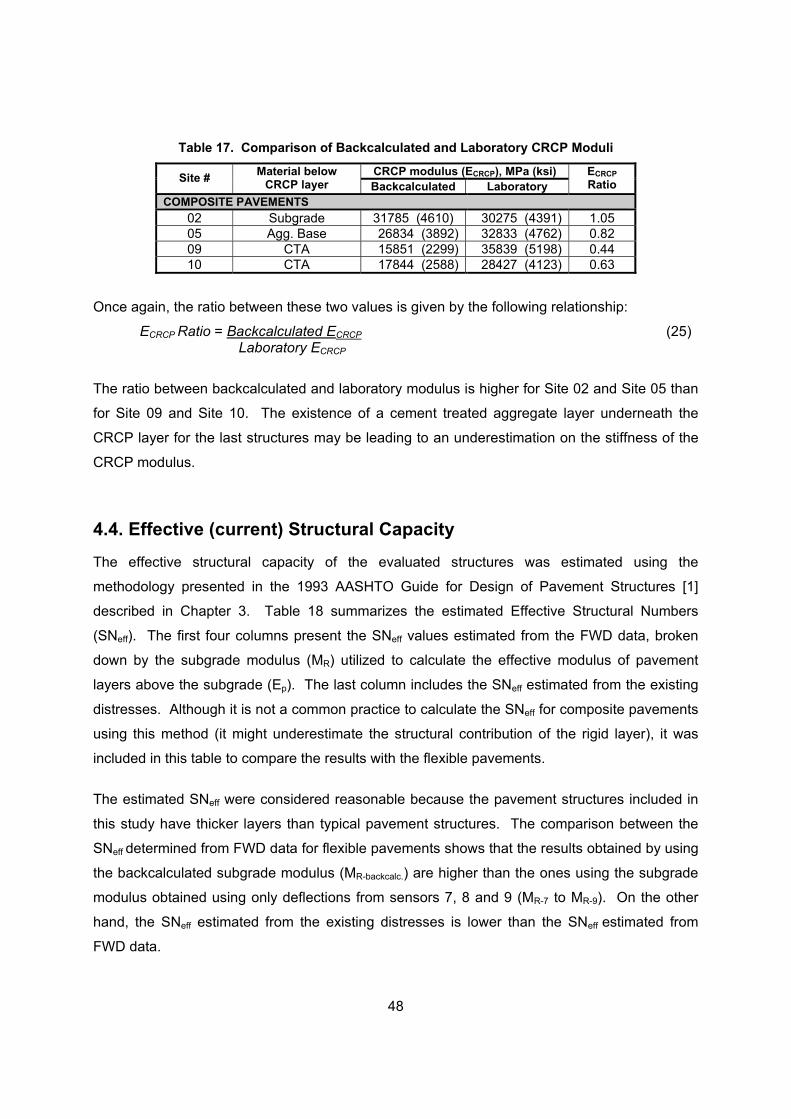
48
Table 17. Comparison of Backcalculated and Laboratory CRCP Moduli
CRCP modulus (ECRCP), MPa (ksi) Site # Material below CRCP layer Backcalculated Laboratory
ECRCP Ratio
COMPOSITE PAVEMENTS 02 Subgrade 31785 (4610) 30275 (4391) 1.05 05 Agg. Base 26834 (3892) 32833 (4762) 0.82 09 CTA 15851 (2299) 35839 (5198) 0.44 10 CTA 17844 (2588) 28427 (4123) 0.63
Once again, the ratio between these two values is given by the following relationship:
ECRCP Ratio = Backcalculated ECRCP Laboratory ECRCP
(25)
The ratio between backcalculated and laboratory modulus is higher for Site 02 and Site 05 than
for Site 09 and Site 10. The existence of a cement treated aggregate layer underneath the
CRCP layer for the last structures may be leading to an underestimation on the stiffness of the
CRCP modulus.
4.4. Effective (current) Structural Capacity
The effective structural capacity of the evaluated structures was estimated using the
methodology presented in the 1993 AASHTO Guide for Design of Pavement Structures [1]
described in Chapter 3. Table 18 summarizes the estimated Effective Structural Numbers
(SNeff). The first four columns present the SNeff values estimated from the FWD data, broken
down by the subgrade modulus (MR) utilized to calculate the effective modulus of pavement
layers above the subgrade (Ep). The last column includes the SNeff estimated from the existing
distresses. Although it is not a common practice to calculate the SNeff for composite pavements
using this method (it might underestimate the structural contribution of the rigid layer), it was
included in this table to compare the results with the flexible pavements.
The estimated SNeff were considered reasonable because the pavement structures included in
this study have thicker layers than typical pavement structures. The comparison between the
SNeff determined from FWD data for flexible pavements shows that the results obtained by using
the backcalculated subgrade modulus (MR-backcalc.) are higher than the ones using the subgrade
modulus obtained using only deflections from sensors 7, 8 and 9 (MR-7 to MR-9). On the other
hand, the SNeff estimated from the existing distresses is lower than the SNeff estimated from
FWD data.

49
Table 18. Effective Structural Number (SNeff)
SNeff from FWD Data SNeff from Distresses Site #
MR-7 MR-8 MR-9 MR-backcalc.
FLEXIBLE PAVEMENTS 01 5.5 5.4 5.2 6.3 4.8 16 8.3 8.2 8.1 8.9 6.8 18 12.5 12.5 12.5 13.0 9.3
COMPOSITE PAVEMENTS 02 7.8 7.9 7.9 6.3 6.1 05 6.7 6.8 6.8 6.3 6.1 09 8.0 8.2 8.2 7.3 7.0 10 7.8 8.0 8.0 7.2 7.0
MR-7 , MR-8 and MR-9: Estimated subgrade modulus using deflection from sensors 7, 8 and 9, at 1219 mm (48 in), 1524 mm (60 in), and 1829 mm (72 in) from center of loading plate, respectively. MR-backcalc: Subgrade modulus from backcalculation analysis.
For composite pavements the situation changes, the subgrade modulus obtained from empirical
relationships (MR-7 to MR-9) is higher than the one obtained by using the backcalculated
subgrade modulus (MR-backcalc.). The SNeff estimated by using the backcalculated subgrade
modulus (MR-backcalc.) is almost identical to the one estimated from existing distresses.
After calculating SNeff, the estimated traffic that these structures can carry before reaching a
terminal serviceability index of 2.5 was estimated using the equations presented in the 1993
AASHTO Design Guide [1]. The results are presented in Table 19.
Table 19. Effective Slab Thickness (Deff)
Estimated Remaining Traffic, W18 (ESAL) Site # SNeff using MR-backcalc
SNeff from Distresses
FLEXIBLE PAVEMENTS 01 3.82 x 10⁷ 4.95 x 10⁶ 16 4.13 x 10⁹ 4.58 x 10⁸ 18 1.85 x 10¹¹ 1.05 x 10¹⁰
COMPOSITE PAVEMENTS 02 2.84 x 10⁸ 2.21 x 10⁸ 05 2.35 x 10⁸ 1.82 x 10⁸ 09 1.22 x 10⁹ 8.71 x 10⁸ 10 1.78 x 10⁹ 1.42 x 10⁹
The structural adequacy of the composite pavements was also estimated in terms of Effective
Slab Thickness (Deff), as shown in Table 20. This value is composed by the thickness of the
rigid layer reduced based on the observed distresses, and a relative contribution of the asphalt

50
layer (which contributes approximately 50% per inch of the rigid layer structural capacity), as
presented in equation (7). This table also presents the estimated remaining traffic that these
structures can carry before reaching a terminal serviceability index of 2.5.
Table 20. Effective Slab Thickness (Deff)
Site # Effective Slab Thickness (Deff), in
Estimated Remaining Traffic,
W18 (ESAL) COMPOSITE PAVEMENTS
02 9.5 2.97 x 10⁸ 05 9.1 2.24 x 10⁸ 09 9.3 2.58 x 10⁸ 10 9.0 2.08 x 10⁸
4.5. M-E Design Guide Software Results
The two types of analysis performed to each of the selected pavement structures using the M-E
Design Guide Software included: (1) New pavement design: from the construction year until the
overlay, and (2) Pavement Rehabilitation: after the overlay (see Section 3.2.6. for more details).
The summary of the results from these analyses are presented in this section; Appendix D
contains the output tables and plots obtained from the software.
4.5.1. Initial Construction
Figure 16 and Figure 17 present a summary of the distresses predicted by the M-E Design
Guide Software from the construction year to the overlay year for flexible pavements and
composite pavements, respectively. The predicted distresses for flexible pavements include
longitudinal surface-down fatigue cracking, bottom-up (alligator) fatigue cracking, thermal
cracking, total rutting, and roughness (in terms of IRI). The predicted distresses for composite
pavements include punchouts (these structures were originally CRCP sections), and roughness.
To identify the critical type of predicted distress(es), all types of distresses were plotted in the
same figure. In order to plot them together (even when they have different units) the
percentage of the distress limit reached in the overlay year was used by applying the following
equation: % Distress Limit = Distress in overlay year x 100 Distress limit
(26)

51
0%
10%
20%
30%
40%
50%
60%
70%
80%
90%
100%
% o
f Dis
tres
s Li
mit
Surf-Down Bott-Up Thermal Tot-Rut IRIDistresses
SITE-01 (23 years)SITE-16 (26 years)SITE-18 (3 years)
Figure 16. Summary of Predicted Distresses from Construction to Overlay Year (Flexible)
It is important to note that the inputs for the AC mix properties were specified volumetric and
default values (Level 3 input level). No AC modulus is necessary as an input for this level.
Figure 16 shows that the most critical predicted distress for flexible pavements were the
following:
- Rutting: reaching 90% of the distress limit for Site 01, 76% for Site 16, and 35% for
Site 18.
- Roughness (IRI): 83% of the limit for Site 16, and 65% for Site 18,
- Surface-down longitudinal fatigue cracking: approximately 55% for Site 16 and Site
18, and 32% for Site 01.
- Thermal cracking: Predicted to affect only Site 18.
- Bottom-up fatigue (alligator) cracking: Reaching no more than 5% of the distress limit
for all the flexible pavements.
The predicted condition for Site 18 was not expected to be that deficient given that the structure
is only three years old. However, this could be consistent with the actual condition; considering
that the structure was overlaid just three years after construction. There is not enough evidence
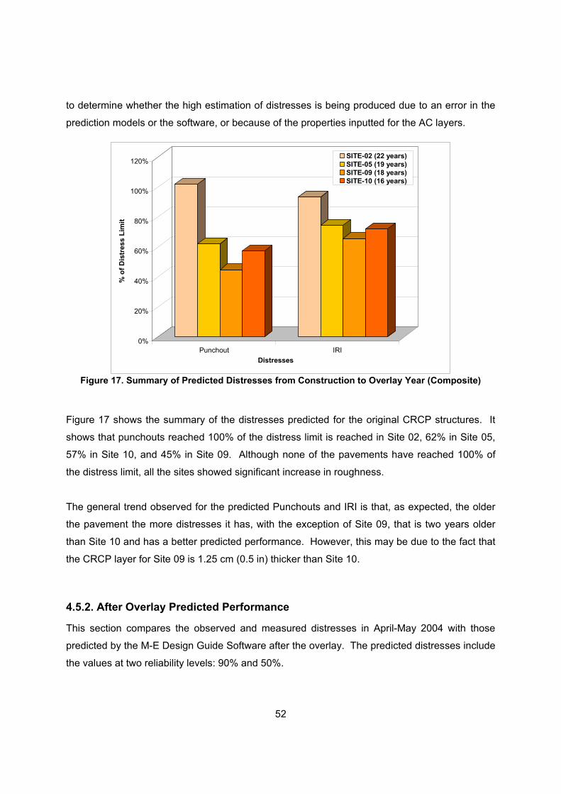
52
0%
20%
40%
60%
80%
100%
120%
% o
f Dis
tres
s Li
mit
Punchout IRIDistresses
SITE-02 (22 years)SITE-05 (19 years)SITE-09 (18 years)SITE-10 (16 years)
to determine whether the high estimation of distresses is being produced due to an error in the
prediction models or the software, or because of the properties inputted for the AC layers.
Figure 17. Summary of Predicted Distresses from Construction to Overlay Year (Composite)
Figure 17 shows the summary of the distresses predicted for the original CRCP structures. It
shows that punchouts reached 100% of the distress limit is reached in Site 02, 62% in Site 05,
57% in Site 10, and 45% in Site 09. Although none of the pavements have reached 100% of
the distress limit, all the sites showed significant increase in roughness.
The general trend observed for the predicted Punchouts and IRI is that, as expected, the older
the pavement the more distresses it has, with the exception of Site 09, that is two years older
than Site 10 and has a better predicted performance. However, this may be due to the fact that
the CRCP layer for Site 09 is 1.25 cm (0.5 in) thicker than Site 10.
4.5.2. After Overlay Predicted Performance
This section compares the observed and measured distresses in April-May 2004 with those
predicted by the M-E Design Guide Software after the overlay. The predicted distresses include
the values at two reliability levels: 90% and 50%.

53
0
50
100
150
200
250
300
350
400
450
500
Surf
ace-
Dow
n Lo
ngitu
dina
l Cra
ckin
g (m
/km
)
1 16 18 2 5 9 10Site Number
Existing Distress
Predicted Distress @ 90%ReliabilityPredicted Distres @ 50%Reliability
Comparison of Measured and Predicted Performance
Surface-down (longitudinal) fatigue cracking is believed to be caused by high shear pressures
developed on the pavement’s surface at the edge of the wheels [10]. The longitudinal cracks
measured from the visual survey included mostly cracks outside the wheelpaths, but very close
to the edges of the wheelpath. These were counted as surface-down cracking in order to
compare them with the software’s output. Figure 18 compares the observed and predicted
surface-down cracks in all sections. The measured transverse cracks account for less than
56.8 m/km (300 ft/mi) in all evaluated sites. While the predicted surface-down cracking at 90%
reliability in flexible Site 01 (eleven-year-old overlay) is relatively close to the observed cracks;
the predicted surface-down cracking is heavily overestimated in the other two flexible sections
(more than 10 and 20 times for Site 16 and Site 18, respectively).
The predictions at 90% reliability for the composite pavements showed better results in
comparison to flexible pavements, with the exception of Site 10, where the predicted surface-
down cracking is more than 4 times the observed cracks. However, these predicted distresses
show an almost constant value of 49 m/km for (258 ft/mi) for all composite pavements, which is
probably the minimum for this reliability level. No distresses were predicted at 50% reliability,
with the exception of Site 16, where the predicted distress is very close to the observed distress.
Figure 18. Predicted vs. Current Distresses – Surface-Down (longitudinal) Fatigue Cracking (m/km)

54
0.00
0.10
0.20
0.30
0.40
0.50
0.60
0.70
0.80
0.90
1.00
1.10
Bot
tom
-Up
Cra
ckin
g (%
of l
ane
area
)
1 16 18 2 5 9 10Site Number
Existing Distress
Predicted Distress @ 90% Reliability
Predicted Distress @50% Reliability
Figure 19 compares the predicted and observed bottom-up (alligator) fatigue cracking. In all
cases the predicted and observed cracking are minimal. Sites 01 (flexible) and 05 (composite)
are the sites affected the most by this type of distress (0.51% and 0.41% respectively). These
values are far from reaching the limit value of 25% of lane area affected by alligator cracking.
The model predicted no distress at 50% reliability level, and an almost constant value of 0.71%
at 90% reliability, probably because this is the minimum value for this reliability level.
Figure 19. Predicted vs. Current Distresses – Bottom-Up (alligator) Fatigue Cracking (% of Lane Area)
Because of its geographic location, thermal cracking is not likely to be a severe problem in
pavements within the Commonwealth of Virginia. However, some transverse cracks were
measured in the visual survey (Figure 20), as described:
- Site 01 (flexible) has the most transverse cracking (59 m/km (312 ft/mi) of potentially
thermal cracking).
- Sites 09, 05, and 02 (all composite) showed 29.5, 22.7, and 17 m/km (156, 120, and
90 ft/mi) of transverse cracking, respectively; however, these cracks might be
reflective cracks from the CRCP layer.
- Site 10 (composite) has a lower number of transverse cracks per mile (4.55 m/km
(24 ft/mi)) than the rest of the composite pavements, probably because its asphalt
surface mix is a Stone Matrix Asphalt (SMA). This type of mix is known to have

55
0
10
20
30
40
50
60
Ther
mal
Cra
ckin
g (m
/km
)
1 16 18 2 5 9 10Site Number
Existing Distress
Predicted Distress @ 90% Reliability
Predicted Distress @ 50% Reliability
greater asphalt content than regular mixes, and uses modified binder. Once again,
these cracks might be reflective cracks from the CRCP layer underneath the AC
surface.
- Site 18 (flexible): this Site does not have any existing transverse cracks because it
has a relatively new overlay (3 years).
Figure 20. Predicted vs. Current Distresses – Thermal Cracking (m/km)
The M-E Design Software predicted no distress at 50% reliability level, with the exception of Site
01, and a constant value of 2.77 m/km (14.6 ft/mi) at 90% reliability in almost all the projects
(with the exception of Site 01), independently of the type of structure, age, or geographic
location; this may be because the predicted distress is so low that the output is showing a
minimum value for all the evaluated sites.
Figure 21 compares the measured and predicted total rutting (defined as the summation of the
rutting in AC layers, unbound base and subgrade) for the seven evaluated sites.

56
0.0
0.2
0.4
0.6
0.8
1.0
1.2
1.4
1.6
1.8
2.0
Tota
l Rut
ting
(cm
)
1 16 18 2 5 9Site Number
Existing Distress
Predicted Distress @ 90% Reliability
Predicted Distress @ 50% Reliability
Figure 21. Predicted vs. Current Distresses – Total Rutting (cm)
The following observations can be drawn from the figure:
- Even in the flexible pavement most affected by rutting (Site 01), the measured rut
depth is only 30 mm (0.12 in) thirteen years after applying the overlay. This can be
considered as an outstanding performance considering that this value is almost 6
times less than the rutting allowable limit of 1.91 cm (0.75 in).
- The composite pavements also show good performance even though they show
slightly higher measured ruts of 69 mm (0.27 in) and 56 mm (0.22 in) for Sites 05 and
02 respectively.
- The predicted results show higher levels of ruts depth for all of the Sites; the output
files from the software analysis indicate that the total rutting for all the Sites is mainly
produced by the deformation of the AC layer.
One of the reasons why the software is predicting higher rutting for the AC layers could be
because the properties of these layers were inputted as Level 3 (default values, see Section
2.5.1.). These include the aggregate gradation of the asphalt mix, the binder’s grade, and
general volumetric properties such as effective binder content, air voids and total unit weight,
etc. The software help indicates that direct inputs of the strength or stiffness of the asphalt mix

57
0.00
0.50
1.00
1.50
2.00
2.50
3.00
3.50
4.00
4.50
5.00
5.50
IRI (
m/k
m)
1 16 18 2 5 9 10Site Number
Existing Distress
Predicted Distress @ 90% Reliability
Predicted Distress @ 50% Reliability
or binder can be input at Level 1 and Level 2. The user can input the results from the dynamic
modulus test, and specific properties of the binder’s grade (softening point, absolute and
kinematic viscosity, specific gravity, penetration, etc.). However, Level 3 was used for the
asphalt layer properties because no dynamic modulus tests were performed to the asphalt
cores, and the software crashed when trying to input asphalt properties of similar mixes as
Level 1.
The smoothness of the pavement structures was measured in terms of the International
Roughness Index (IRI), as shown in Figure 22.
Figure 22. Predicted vs. Current Distresses – IRI (m/km)
The analysis of this figure is presented following:
- Site 01 is the flexible pavement site with the highest measured IRI value of 1.53
m/km (96.9 in/mi), followed by Site 18 with 1.15 m/km (72.8 in/mi), and Site 16 with
0.64 m/km (43 in/mi).
- The measured IRI is similar for the four composite pavement sites, having a value of
1.37 m/km (87.1 in/mi) for Site 02, 1.31 m/km (82.8 in/mi) for Site 09, 1.19 m/km
(75.3 in/mi) for Site 05, and 1.04 m/km (66.0 in/mi) for Site 10.
- These IRI values show that all the sites are performing satisfactorily, considering that
some agencies accept an IRI value of 1.26 m/km (80 in/mi) for new structures [20],

58
and that most of the evaluated pavements have a surface layer at least five years
old.
- The predicted IRI for flexible pavements at 90% reliability are higher than the
measured values, especially for Sites 01 and 16.
- In the case of composite pavements, the predicted values at 90% reliability closer to
the measured IRI.
- The predicted IRI for flexible and composite pavements at 50% reliability are very
close to the measured IRI, with the exception of flexible Sites 01 and 16.
Critical Distress Identification
In order to identify the critical type of distress(es) affecting the pavement structures investigated,
Figure 23 was created.
Similarly to the previous section, all the types of distresses for all Sites were plotted in the same
figure. The percentage of the distress limit reached in year 2004 was computed using the
following equation:
% Distress Limit in 2004 = Distress in 2004 x 100 Distress limit
(27)
Figure 23 depicts the flexible pavements in different blue tones, while the composite pavements
are shaded with orange colors. One of the first things that can be seen from this figure is that
most of the distresses have not reached 50% of the threshold. The most critical distress for
flexible pavements is again surface-down cracking, followed by thermal cracking, total rutting,
and bottom-up fatigue cracking.
A detailed analysis of the observed and measured distresses in 2004 is presented following:
- Site 01 (flexible): is the flexible pavement in the worst general condition. It is
important to remember that this structure is 34 years old and was overlaid 11 years
ago.
- Site 16 (flexible) has an older overlay (13 years) and higher traffic level than Site 01
but shows better performance. Even though no historical data on the previous
pavement pre-overlay condition is available. Site 16 may be performing better

59
0%
10%
20%
30%
40%
50%
60%
70%
80%
90%
100%
% o
f Dis
tres
s Li
mit
Surf-Down Bott-Up Thermal Tot-Rut IRIDistresses
SITE-01SITE-16SITE-18SITE-02SITE-05SITE-09SITE-10
because its AC layer is 5 cm (2 in) thicker than Site 01, and because it has a thick
aggregate layer of 43 cm (18 in) in comparison to 15 cm (6 in) of Cement Treated
Aggregate for Site 01.
- The observed critical distresses for flexible pavements are: bottom-up cracking (Site
02), total rutting (Sites 02 and 05), surface-down fatigue cracking (Sites 05, 09, and
02), and thermal cracking (Sites 05 and 02) in decreasing order.
- The composite pavements in the worst general condition are Site 05 and Site 02.
These sites have the highest measured rutting.
- Even though Sites 09 and 10 have similar structure, similar age and are located
close from each other, Site 10 is performing better even with a higher level of traffic.
It is suspected that the enhanced performance is due to the SMA surface used on
this Site.
Figure 23. Summary of Existing Distresses in 2004
4.6. M-E Design Guide Software Limitations and Troubleshooting
During the analysis, some problems and limitations with the software were encountered.
However, time constrains of the project did not allow to conduct a detailed evaluation of the
software, or a thorough troubleshooting of the problems encountered. Some of the problems
are listed as follows:

60
- If traffic opening month is not one month after the CRCP is placed, the program will give
an error with the punchout model.
- When the rehabilitation analysis was performed for a relatively complex structure, or for
a long life period (greater than 20 years), the program crashed and the following error
message prompted out: “Error – Failure to open modulus.tmp and fatigue.tmp. Apads
MFC. Application has encountered a problem and needs to close. We are sorry for any
inconvenience”.
- It was observed that in the Rehabilitation Levels 2 and 3 it is allowed to enter the
backcalculated layer moduli for the asphalt layers (even for Level 3 Input); however,
unreasonable results were obtained, i.e. the predicted asphalt moduli were extremely
low, consequently, a high occurrence of distresses was predicted. The results
presented on this thesis are based on the use of Rehabilitation Level 3 without allowing
the input of the backcalculated layer moduli for the asphalt layers in Level 3 Input,
therefore just default values and values established in road construction specifications
were used, making the results less accurate.
- When trying to input the asphalt properties as Level 1 Input the following error occurred:
“Modulus.exe has encountered a problem and needs to close”.
- The program was not able to estimate the IRI for a structure with an AC surface over a
CTA layer. It is believed that this happened because the fatigue model for the
chemically stabilized layer is not yet calibrated.
- The IRI model was not sensitive to different structures and ages; it appeared to be using
default values.

61
Chapter 5 - FINDINGS AND CONCLUSIONS The structural analysis of three flexible and four composite pavement structures allowed
determining the structural adequacy of each of the pavement structures. This analysis also
provided some of the inputs required to predict pavement performance using the M-E Design
Guide Software. The comparison of the measured and predicted distresses allowed a
preliminary verification of the M-E Design Guide capabilities and the adequacy of its models for
predicting the performance of pavement structures in the Commonwealth of Virginia. This
chapter presents the main findings and conclusion from the investigation.
5.1. Findings
Following are the main findings concerning the structural adequacy of the evaluated pavement
sections, and the verification of the M-E Design Guide Software:
• The amount of observed and measured distresses was not significant in most of the
evaluated flexible and composite pavements. The evaluated sections fitted into the
adequate condition level for the different types of measured distresses, with the only
exception of composite Site 05, with a marginal level for longitudinal cracking.
• In general, the backcalculation process presented some difficulties because of the
complexity of some of the structures evaluated, especially the composite pavements.
The problems are believed to be due to departure from some of the assumptions used
by the software, e.g. moduli not decreasing with depth, and compensating errors. In
addition, the thin HMA surface layers had to be combined with the HMA base.
- The backcalculation for the flexible pavements produced reasonable moduli for all
the pavement layers and good RMS error values (ranging from 3.0% to 3.2%).
- The results achieved for the composite sections were also considered reasonable
and the RMS error was lower than for the flexible pavements (1.6% to 3.0%).
However, the backcalculated moduli for the asphalt layers were relatively low.
- The backcalculated subgrade moduli were in general higher than the typical values
reported in the literature. The computed values were 1.5 times higher than the

62
average typical modulus for silty soils, and 2.8 times higher than the average
typical modulus for clayey soils.
- The backcalculated HMA moduli were generally lower than the resilient modulus
obtained in the laboratory (with the exception of Site 10).
- The backcalculated modulus of the CRCP section was similar to the modulus
estimated from compressive strength test on extracted cores for the composite
pavements without an ATB layer, but the backcalculated moduli were lower than
the lab results in the case of composite pavements with an ATB layer.
• The visual survey conducted in 2004 suggests that the most critical distress for the
flexible pavements is longitudinal (probably surface-down) cracking, followed by rutting
and transversal (thermal) cracking. For the composite pavements, the most critical
distress was rutting, followed by longitudinal (probably surface-down) cracking, and
transversal (thermal) cracking. No significant amount of bottom-up (alligator) cracking
was observed in any of the evaluated sections.
• The estimation of the effective structural adequacy (in terms of SNeff for flexible and
Deff for composite pavements) shows that the evaluated sites are structurally sound.
• The distresses predicted by the M-E Design Software at 90% reliability were in general
higher than those measured on the overlaid pavements. On the other hand, minimal
or no surface-down, bottom-up fatigue, or thermal cracking were predicted at 50%
reliability on any of the sites.
• The predicted IRI for flexible and composite pavements at 50% reliability are very
close to the measured IRI, with the exception of flexible Sites 01 and 16.
5.2. Conclusions
The in-depth structural evaluation of the three flexible and four composite pavements showed
that all the sites are structurally sound. The investigation also confirmed that the use of GPR to
determine layer thicknesses and the comparison with a minimum number of cores is a helpful
tool for pavement structural evaluation. Despite some difficulties performing the backcalculation
analysis for complex structures, the obtained results were considered reasonable and were
useful in estimating the current structural adequacy of the evaluated structures.
The comparison of the measured distresses with those predicted by the M-E Design Guide
software showed poor agreement. In general, the predicted distresses were higher than the

63
distresses actually measured. However, there was not enough evidence to determine whether
this is due to errors in the prediction models or software, or because of the use of defaults
material properties, specially for the AC layers. It must be noted that although an in-depth field
evaluation was performed, only Level 3 data was available for many of the input parameters.
The results suggest that significant calibration and validation will be required before
implementation of the M-E Design Guide.

64
Chapter 6 - RECOMMENDATIONS The recommendations included in this Chapter are intended to enhance the data collection and
analysis process for future in-depth field evaluations, as well as to improve the understanding of
the use of the M-E Design Guide Software.
Recommendations for Data Collection
The extensive filed investigations allowed recommending some potential improvements to the
pavement evaluation procedures that may be applied in future similar projects:
• In order to determine the thickness of the existing layers accurately it is
recommended to keep comparing the thicknesses obtained from the coring process,
GPR, and Historical Data because these methods complement each other.
• It would be useful to perform some basic strength tests on the granular layers and
subgrade to obtain more information about these layers because the historical data
is not always available and/or reliable. A simple device that allows estimating the
CBR and resilient modulus values is, for example, the Dynamic Cone Penetrometer
[11], [16].
• To understand the behavior of the subgrade soil it is recommended to at least run a
complete soil classification. The gradation and type of subgrade are also important
inputs required to perform the analysis using the M-E Design Software.
• Having historical records of the condition of the road before applying the overlay, as
well as measurements of the longitudinal and transverse profiles before and after the
overlay could help in understanding the development of current distresses and
pavement performance.
• Despite the difficulties with the FWD backcalculation for complex pavement
structures, it is recommended to continue using this method to estimate layer moduli
and the structural adequacy of the pavement structure.

65
Recommendation for Future Research
The national calibration factors used on the distress prediction models do not seem to apply to
the structures considered for this thesis. Calibration of the performance models to the
conditions in the Commonwealth of Virginia is recommended.
It is suspected that the predicted results achieved from the M-E Design Software were affected
by the default asphalt layer properties used. The input information used was mostly default
values and typical values specified by the Commonwealth of Virginia (input Level 3), even after
performing an in-depth evaluation. It is recommended to perform a complete characterization of
the AC materials (including dynamic modulus, volumetric properties, etc.) to asses the effect of
using measured properties on the prediction of pavement performance.

66
References
[1] American Association for State Highway and Transportation Officials (AASHTO), “Guide
for Design of Pavement Structures”, 1993.
[2] ASCE, ASCE Renewing America’s Infrastructure – A Citizen’s Guide – Report Card for
America’s Infrastructure, http://www.asce.org/reportcard/2005/page.cfm?id=30
[3] Bredenhann, S., and van de Ven, M., Application of Artificial Neural Networks in the Back-
Calculation of Flexible pavement Layer Moduli from Deflection Measurements, In 8th
Conference on Asphalt Pavements for Southern Africa (CAPSA ’04), ISBN Number 1-920-
01718-6, Sun City, South Africa, September 2004.
[4] Cost - Transport, Final Draft Report of COST Action 336 – Falling Weight Deflectometer,
Lisbon, June 1999.
[5] Dynatest, ELMOD 4 for Windows, http://www.dynatest.com/software/elmod_4.htm#.
[6] Federal Highway Administration, Temperature Predictions and Adjustment Factors for
Asphalt Pavement, Publication No. FHWA-RD-98-085, Virginia, June, 2000.
[7] Flintsch, G., Appea, A., Al-Qadi, I., and Loulizi, A., “Backcalculation Validation Through
Field Instrumentation Response at the Virginia Smart Road”, Virginia Tech Transportation
Institute, presented for the Second International Symposium on Maintenance and
Rehabilitation of Pavements and Technological Control, Auburn, Alabama, USA.
[8] Foinquinos, R., Roesset, J. and Stokoe II, K., Response of Pavement Systems to Dynamic
Loads Imposed by Nondestructive Tests, Transportation Research Record 1504, pp 57-67,
1995.
[9] George, K., Soil Stabilization Field Trial - Interim Report III. Department of Civil
Engineering, University of Mississippi, November, 2003.

67
[10] Guide for Mechanistic-Empirical Design of New and Rehabilitated Pavement Structures –
Final Report (1-37A), National Cooperative Highway Research Program (NCHRP),
Transportation Research Board (TRB) and National Research Council (NRC), March 2004.
[11] Herath, A., et al., The Use of Dynamic Cone Penetrometer to Predict Resilient Modulus of
Subgrade Soils.
[12] Hoffman, M. S., and M. R. Thompson. Comparative Study of Selected Nondestructive
Devices. Transportation Research Record 1293, TRB, National Research Council,
Washington, DC, 1991, pp. 12-23.
[13] Hudson, R., Haas, R., and Uddin, W., “Infrastructure Management: Integrating Design,
Construction, Maintenance, Rehabilitation, Renovation”, McGraw Hill, United States of
America, 1997.
[14] Li, Y., and Nazarian, L., Evaluation of Aging of Hot Mix Asphalt Using Wave Propagation
Techniques. In STP 1265, ASTM, Philadelphia, PA, 1994.
[15] Mehta, Y., and Roque, R., “Evaluation of FWD Data for Determination of Layer Moduli of
Pavements, ASCE Journal of Materials in Civil Engineering, Vol. 15, No. 1, Feb 1 2003.
[16] Minnesota Department of Transportation, User Guide to the Dynamic Cone Penetrometer,
Office of Minnesota Road Research, Minnesota, 1996, 20 pp.
[17] Saeed, A., and Hall, J., Comparison of Non-Destructive Testing Devices to Determine In-
Situ Properties of Asphalt Concrete Pavement Layers, Transportation Research Board,
Washington, D.C., 2003.
[18] Strategic Highway Research Program, “SHRP’s Layer Moduli Backcalculation Procedure
(SHRP-P-655)”, National Research Council, Washington, DC 1993.
[19] Ullidtz, P., Coetzee, N., Analytical Procedures in Nondestructive Testing Pavement
Evaluation. In Transportation Research Record 1482. Transportation Research Board,
Washington, D.C., 1995.

68
[20] US Army Corps of Engineers and Federal Aviation Administration, Hot-Mix Asphalt Paving
Handbook 2000.
[21] Virginia Department of Transportation, A Guide To Evaluating Pavement Distress Through
The Use Of Video Images, Maintenance Division, Revised on 08/23/01.
[22] Virginia Department of Transportation, Development and Implementation of Pavement
Condition Indices for the Virginia Department of Transportation (Phase I and II, Flexible
and Rigid Pavements), Maintenance Division, 2002.
[23] Virginia Department of Transportation, Road and Bridge Specifications for the
Commonwealth of Virginia, Richmond, July 1982.
[24] Virginia Department of Transportation, Road and Bridge Specifications for the
Commonwealth of Virginia, Richmond, January 1991.
[25] Virginia Department of Transportation, Road and Bridge Specifications for the
Commonwealth of Virginia, Richmond, January 1994.
[26] Virginia Department of Transportation, Road and Bridge Specifications for the
Commonwealth of Virginia, Richmond, 2002.
[27] Virginia Department of Transportation, TAG User’s Manual and Technical Documentation,
Version 1.0, Materials Division – Pavement Design and Evaluation Section, November
2001.
[28] Washington Department of Transportation (WSDOT), Pavement Guide – Pavement
Analysis Computer Software and Case Studies, Volume 3, Washington State, February
1995.

69
Appendix A – Determination of Layer Thickness from Cores, GPR, and Historical Data

70
Appendix A – Determination of Layer Thicknesses from Cores, GPR, and Historical Data
FLEXIBLE PAVEMENTS:
Table A-1. Site 01 (Flexible)
HISTORICAL DATA GPR CORES Layer
# Material Thickness mm (in) Year Material Thickness
mm (in) Material Thickness mm (in)
1 SM-2A 38 (1.5) 1993 2 S-6 30 (1.2) 1981
SM2A + S6 58 (2.3) Surface
Mix 115 (4.5)
3 S-5 unknown 1970 S-5 198.1 (7.8) Base Mix 125 (4.9)
4 - - - - - Cement Treated Aggregate
150 (5.9)
4 Subgrade - - Subgrade - Subgrade - SM: Asphalt surface mix layer; S: Asphalt surface layer NOTE: Shaded area indicates the thickness selected for each layer
Table A-2. Site 16 (Flexible)
HISTORICAL DATA GPR CORES Layer
# Material Thickness mm (in) Year Material Thickness
mm (in)) Material Thickness mm (in)
1 SM-2C 46 (1.8) 1991 SM-2C
48.2 (1.9) Surface Mix
39 (1.5)
2 I-3 10 (0.4) 1965
3 CB-1 or H-2 33 (1.3) -
4 H-3 191 (7.5) -
I3 + CB1 + H3 233 (9.2) Base Mix 256 (10.1)
5 Aggregate Base Type 1
152 (6.0) - Aggregate Base 125.4 (4.9) - -
6 Select Material Type 1
305 (12.0) - - - - -
7 Subgrade - - Subgrade - Subgrade - SM: Asphalt surface mix layer; I: Asphalt intermediate layer; CB: Asphalt base layer; H: Asphalt base layer
NOTE: Shaded area indicates the thickness selected for each layer

71
Table A-3. Site 18 (Flexible)
HISTORICAL DATA GPR CORES Layer
# Material Thickness mm (in) Year Material Thickness
mm (in) Material Thickness mm (in)
1 SM-2A 51(2.0) 2001 SM2B 58.9 (2.3) Surface Mix 55 (2.2)
2 IM-1A 64 (2.5) 1999 IM1A 30.1(1.2) 3 BM-3 254 (10.0) 1999 BM3 246.9 (9.7)
Base Mix (IM + BM) 319 (12.6)
4 OGDL-Type1 (2%)
76 (3.0) 1999 OGDL 51.4 (2.0) OGDL (asphalt) 70 (2.8)
5 21B 533 (21.0) 1999 - - - - 6 Subgrade - - Subgrade - Subgrade -
SM: Asphalt surface mix layer; IM: Asphalt intermediate mix layer; BM: Asphalt base mix layer; OGDL: Open graded drainage layer; 21B: Aggregate base layer NOTE: Shaded area indicates the thickness selected for each layer
COMPOSITE PAVEMENTS:
Table A-4. Site 02 (Composite)
HISTORICAL DATA GPR CORES Layer
# Material Thickness mm (in) Year Material Thickness
mm (in) Material Thickness mm (in)
1 SM-2C 38 (1.5) 1992 SM-2C 51.7 (2.0) Surface Mix 41(1.6)
2 BM-2 74 (2.9) 1992 BM-2 70.9 (2.8) Base Mix 74 (2.9) 3 CRCP 203 (8.0) 1970 CRCP 159.8 (6.3) CRCP 209 (8.2) 4 Subgrade - - Subgrade - Subgrade -
SM: Asphalt surface mix layer; BM: Asphalt base mix layer; CRCP: Continuously reinforced concrete pavement NOTE: Shaded area indicates the thickness selected for each layer
Table A-5. Site 05 (Composite)
HISTORICAL DATA GPR CORES Layer
# Material Thickness mm (in) Year Material Thickness
mm (in) Material Thickness mm (in)
1 SM-2C 38 (1.5) 1991 Surface Mix
44 (1.7)
2 IM-1B 102 (4.0) 1990
SM2C + IM1B 115 (4.5)
Base Mix 67 (2.6) 3 CRCP 203 (8.0) 1972 CRCP 196 (7.7)
4 Aggregate Size 22 152 (6.0) 1972
CRCP + Base
339.4 (13.4) - -
5 Subgrade - 1972 - - - - SM: Asphalt surface mix layer; IM: Asphalt intermediate mix layer; CRCP: Continuously reinforced concrete pavement NOTE: Shaded area indicates the thickness selected for each layer

72
Table A-6. Site 09 (Composite)
HISTORICAL DATA GPR CORES Layer
# Material Thickness mm (in) Year Material Thickness
mm (in) Material Thickness mm (in)
1 SM-2D 51(2.0) 1998 SM-2D 87.6 (3.4) Surface 95 (3.7) 2 CRCP 203 (8.0) 1980 CRCP 244.2 (9.6) CRCP 216 (8.5) 3 21A (4%) 152 (6.0) 1980 - - - - 4 Subgrade - - Subgrade - Subgrade -
SM: Asphalt surface mix layer; 21A: Cement treated aggregate layer; CRCP: Continuously reinforced concrete pavement NOTE: Shaded area indicates the thickness selected for each layer
Table A-7. Site 10 (Composite)
HISTORICAL DATA GPR CORES Layer
# Material Thickness mm (in) Year Material Thickness
mm (in) Material Thickness mm (in)
1 SMA 38 (1.5) 1996 Surface Mix 40 (1.6)
2 IM-1A 51(2.0) 1996
SMA + IM1A 99.3 (3.9)
Base Mix 59 (2.3) 3 CRCP 203 (8.0) - CRCP 211.5 (8.3) CRCP 203 (8.0) 4 CTA 152 (6.0) - - - - - 5 Subgrade - - Subgrade - Subgrade -
SM: Asphalt surface mix layer; IM: Asphalt intermediate mix layer; CRCP: Continuously reinforced concrete pavement; CTA: Cement treated aggregate NOTE: Shaded area indicates the thickness selected for each layer

73
Appendix B – Homogeneous Sections Based on Cumulative Sums of Deflections

74
-0.110
-0.090
-0.070
-0.050
-0.030
-0.010
0.010
0.030
0.050
0.070
0 100 200 300 400 500 600 700 800 900
Distance (m)
Cum
ulat
ive
Sum
of D
efle
ctio
n - S
ite 0
1
Sensor 1 (0 mm from loading plate)
Sensor 7 (1219 mm from loading plate)
Selected Homogeneous Sections
-0.080
-0.060
-0.040
-0.020
0.000
0.020
0.040
0 100 200 300 400 500 600 700 800
Distance (m)
Cum
ulat
ive
Sum
of D
efle
ctio
n - S
ite 1
6
Sensor 1(0 mm from loading plate)
Sensor 7 (1219 mm from loading plate)
Selected Homogeneous Sections
Appendix B – Homogeneous Sections Based on
Cumulative Sums of Deflections
FLEXIBLE PAVEMENTS:
Figure B-1. Homogeneous Sections – Site 01
Figure B-2. Homogeneous Sections – Site 16

75
-0.060
-0.050
-0.040
-0.030
-0.020
-0.010
0.0000 100 200 300 400 500 600 700 800 900
Distance (m)
Cum
ulat
ive
Sum
of D
efle
ctio
n - S
ite 1
8
Sensor 1(0 mm from loading plate)
Sensor 7 (1219 mm from of loading plate)
Selected Homogeneous Sections
-0.070
-0.060
-0.050
-0.040
-0.030
-0.020
-0.010
0.0000 100 200 300 400 500 600 700
Distance (m)
Cum
ulat
ive
Sum
of D
efle
ctio
n - S
ite 0
2
Sensor 1 (0 mm from loading plate)
Sensor 7 (1219 mm from loading plate)
Selected Homogeneous Sections
Figure B-3. Homogeneous Sections – Site 18
COMPOSITE PAVEMENTS:
Figure B-4. Homogeneous Sections – Site 02

76
-0.060
-0.020
0.020
0.060
0.100
0.140
0.180
0 100 200 300 400 500 600 700 800 900
Distance (m)
Cum
ulat
ive
Sum
of D
efle
ctio
n - S
ite 0
5Sensor 1 (0 mm from loading plate)
Sensor 7 (1219 mm from loading plate)
Selected Homogeneous Sections
-0.120
-0.100
-0.080
-0.060
-0.040
-0.020
0.000
0.020
0.040
0 100 200 300 400 500 600 700 800 900
Distance (m)
Cum
ulat
ive
Sum
of D
efle
ctio
ns -
Site
09
Sensor 1 (0 mm from loading plate)
Sensor 7 (1219 from loading plate)
Selected Homogeneous Sections
Figure B-5. Homogeneous Sections – Site 05
Figure B-6. Homogeneous Sections – Site 09

77
-0.010
-0.005
0.000
0.005
0.010
0.015
0.020
0.025
0.030
0.035
0.040
0 100 200 300 400 500 600 700 800 900
Distance (m)
Cum
ulat
ive
Sum
of D
efle
ctio
ns -
Site
10
Sensor 1 (0 mm from loading plate)Sensor 7 (0 mm from loading plate)Selected Homogeneous Sections
Figure B-7. Homogeneous Sections – Site 10

78
Appendix C – Backcalculation Results ELMOD 5.1

79
1
10
100
1,000
10,000
100,000
0 100 200 300 400 500 600 700 800
Distance (m)
Res
ilient
Mod
ulus
(MP
a)
SM + BMCTASubgradeSM (lab)BM (lab)
1
10
100
1,000
10,000
100,000
0 100 200 300 400 500 600 700 800
Distance (m)
Res
ilient
Mod
ulus
(MP
a)
SM + BMAgg. Base + Select MaterialSubgradeSM (lab)BM (lab)
Appendix C – Backcalculation Results ELMOD 5.1
FLEXIBLE PAVEMENTS:
Figure C-1. Backcalculation Results – Site 01
Figure C-2. Backcalculation Results – Site 16
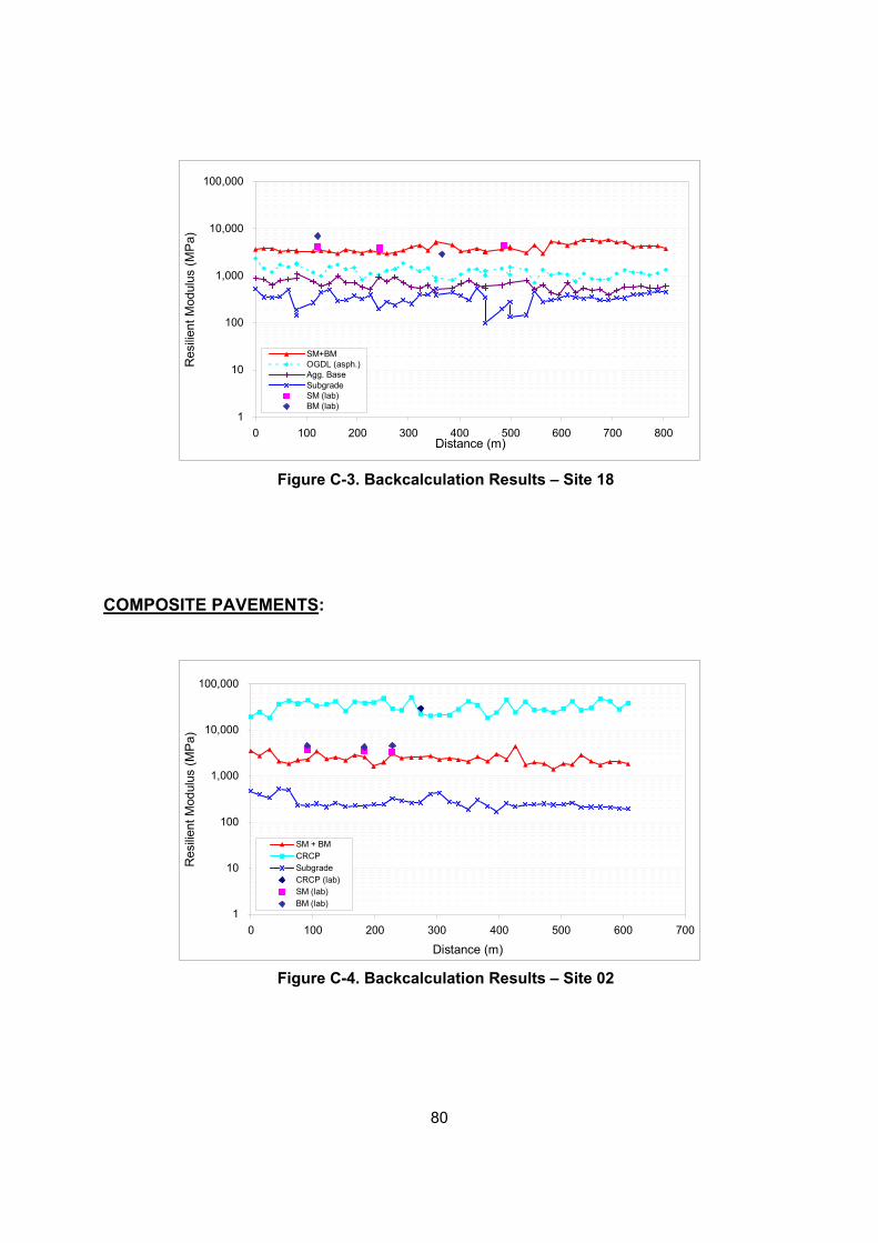
80
1
10
100
1,000
10,000
100,000
0 100 200 300 400 500 600 700 800Distance (m)
Res
ilient
Mod
ulus
(MP
a)
SM+BMOGDL (asph.)Agg. BaseSubgradeSM (lab)BM (lab)
1
10
100
1,000
10,000
100,000
0 100 200 300 400 500 600 700
Distance (m)
Res
ilient
Mod
ulus
(MP
a)
SM + BMCRCPSubgradeCRCP (lab)SM (lab)BM (lab)
Figure C-3. Backcalculation Results – Site 18
COMPOSITE PAVEMENTS:
Figure C-4. Backcalculation Results – Site 02

81
1
10
100
1,000
10,000
100,000
0 100 200 300 400 500 600 700 800
Distance (m)
Res
ilient
Mod
ulus
(MP
a)
SM + BM CRCP
Agg. Base Subgrade
CRCP (lab) SM (lab)
BM (lab)
1
10
100
1,000
10,000
100,000
0 100 200 300 400 500 600 700 800
Distance (m)
Res
ilient
Mod
ulus
(MP
a)
SM + BMCRCPCTASubgradeCRCP (lab)SM (lab)
Figure C-5. Backcalculation Results – Site 05
Figure C-6. Backcalculation Results – Site 09

82
1
10
100
1,000
10,000
100,000
0 100 200 300 400 500 600 700 800Distance (m)
Res
ilient
Mod
ulus
(MP
a)
SM + BM CRCP
CTA Subgrade
CRCP (lab) SM (lab)
BM (lab)
Figure C-7. Backcalculation Results – Site 10

83
Appendix D – M-E Design Software Output

84
Limit Reliability62
172 901000 90
25 901000 90
25 900.25 900.75 90
5802
508060
Class 4 Class 5 Class 6 Class 7 Class 8 Class 9 Class 10 Class 11 Class 12 Class 131.00 1.00 1.00 1.00 1.00 1.00 1.00 1.00 1.00 1.00 1.00 1.00 1.00 1.00 1.00 1.00 1.00 1.00 1.00 1.00 1.00 1.00 1.00 1.00 1.00 1.00 1.00 1.00 1.00 1.00 1.00 1.00 1.00 1.00 1.00 1.00 1.00 1.00 1.00 1.00 1.00 1.00 1.00 1.00 1.00 1.00 1.00 1.00 1.00 1.00 1.00 1.00 1.00 1.00 1.00 1.00 1.00 1.00 1.00 1.00 1.00 1.00 1.00 1.00 1.00 1.00 1.00 1.00 1.00 1.00 1.00 1.00 1.00 1.00 1.00 1.00 1.00 1.00 1.00 1.00 1.00 1.00 1.00 1.00 1.00 1.00 1.00 1.00 1.00 1.00 1.00 1.00 1.00 1.00 1.00 1.00 1.00 1.00 1.00 1.00 1.00 1.00 1.00 1.00 1.00 1.00 1.00 1.00 1.00 1.00 1.00 1.00 1.00 1.00 1.00 1.00 1.00 1.00 1.00 1.00
Midnight 2.3% Noon 5.9%1.3% 1:00 am 2.3% 1:00 pm 5.9%8.5% 2:00 am 2.3% 2:00 pm 5.9%2.8% 3:00 am 2.3% 3:00 pm 5.9%0.3% 4:00 am 2.3% 4:00 pm 4.6%7.6% 5:00 am 2.3% 5:00 pm 4.6%
74.0% 6:00 am 5.0% 6:00 pm 4.6%1.2% 7:00 am 5.0% 7:00 pm 4.6%3.4% 8:00 am 5.0% 8:00 pm 3.1%0.6% 9:00 am 5.0% 9:00 pm 3.1%
Project: SITE01-New Design.dgp
General Information Description:(RUN 1: Original Design) o Route: 29 South o County: Amherst (number 5) o Length: 2640 ft o Number of lanes in each direction: 2 o Pavement Category: Flexible, 10-15 years o Traffic: TT 1,100, AADT 20,000 (one way traffic) o AC overlay 1.5in ; HMA 8in; CTA 6in o Subgrade: wet red, brown, gray sandy silt w/mica, fill material
Design Life 25 yearsBase/Subgrade construction: August, 1970Pavement construction: September, 1970Traffic open: September, 1970Type of design Flexible
Analysis ParametersAnalysis type Probabilistic
Performance CriteriaInitial IRI (in/mi)Terminal IRI (in/mi)AC Surface Down Cracking (Long. Cracking) (ft/500):AC Bottom Up Cracking (Alligator Cracking) (%):AC Thermal Fracture (Transverse Cracking) (ft/mi):Chemically Stabilized Layer (Fatigue Fracture)Permanent Deformation (AC Only) (in):Permanent Deformation (Total Pavement) (in):
Location: SITE 01Project ID: SITE O1Section ID:
Principal Arterials - Interstate and Defense RoutesDate: 2/13/2005
Station/milepost format: Miles: 0.000Station/milepost begin: 7.8Station/milepost end: 7.3Traffic direction: South bound
Default Input LevelDefault input level Level 3, Default and historical agency values.
Traffic Initial two-way aadtt:Number of lanes in design direction:Percent of trucks in design direction (%):Percent of trucks in design lane (%):Operational speed (mph):
Traffic -- Volume Adjustment FactorsMonthly Adjustment Factors (Level 3, Default MAF)
Vehicle ClassMonth
JanuaryFebruaryMarchAprilMayJuneJulyAugustSeptemberOctoberNovemberDecember
Vehicle Class Distribution Hourly truck traffic distribution(Level 3, Default Distribution) by period beginning:
AADTT distribution by vehicle classClass 4Class 5Class 6Class 7Class 8Class 9Class 10Class 11Class 12
Appendix D – M-E Design Software Output

85
4.0%4.0%4.0%4.0%4.0%4.0%4.0%4.0%4.0%4.0%
18
1012
1.62 0.39 0.00 0.00 2.00 0.00 0.00 0.00 1.02 0.99 0.00 0.00 1.00 0.26 0.83 0.00 2.38 0.67 0.00 0.00 1.13 1.93 0.00 0.00 1.19 1.09 0.89 0.00 4.29 0.26 0.06 0.00 3.52 1.14 0.06 0.00 2.15 2.13 0.35 0.00
8.5
12
120120
51.649.249.2
37.57-79.0662823
Traffic Growth Factor
Vehicle Class
Growth Rate
GrowthFunction
Class 4 CompoundClass 5 CompoundClass 6 CompoundClass 7 CompoundClass 8 CompoundClass 9 CompoundClass 10 CompoundClass 11 CompoundClass 12 CompoundClass 13 Compound
Traffic -- Axle Load Distribution FactorsLevel 3: Default
Traffic -- General Traffic InputsMean wheel location (inches from the lane marking):Traffic wander standard deviation (in):Design lane width (ft):
Number of Axles per Truck
Quad Axle
Class 4Class 5Class 6
Vehicle Class
Single Axle
Tandem Axle
Tridem Axle
Class 7Class 8Class 9Class 10Class 11Class 12Class 13
Axle ConfigurationAverage axle width (edge-to-edge) outside dimensions,ft):Dual tire spacing (in):
Axle ConfigurationSingle Tire (psi):Dual Tire (psi):
Average Axle SpacingTandem axle(psi):Tridem axle(psi):Quad axle(psi):
Climate icm file:
site01-01BLatitude (degrees.minutes)Longitude (degrees.minutes)Elevation (ft)Depth of water table (ft)
Structure--Design Features
Structure--Layers Layer 1 -- Asphalt concrete
Material type: Asphalt concreteLayer thickness (in): 3
General PropertiesGeneralReference temperature (F°): 70

86
Volumetric Properties as BuiltEffective binder content (%): 11Air voids (%): 4.3Total unit weight (pcf): 148
Poisson's ratio: 0.35 (user entered)
Thermal PropertiesThermal conductivity asphalt (BTU/hr-ft-F°): 0.67Heat capacity asphalt (BTU/lb-F°): 0.23
Asphalt MixCumulative % Retained 3/4 inch sieve: 0Cumulative % Retained 3/8 inch sieve: 12Cumulative % Retained #4 sieve: 45% Passing #200 sieve: 5
Asphalt BinderOption: Conventional viscosity gradeViscosity Grade AC 20A 10.7709 (correlated)VTS: -3.6017 (correlated)
Layer 2 -- Asphalt concreteMaterial type: Asphalt concreteLayer thickness (in): 5
General PropertiesGeneralReference temperature (F°): 70
Volumetric Properties as BuiltEffective binder content (%): 10Air voids (%): 6Total unit weight (pcf): 162
Poisson's ratio: 0.35 (user entered)
Thermal PropertiesThermal conductivity asphalt (BTU/hr-ft-F°): 0.67Heat capacity asphalt (BTU/lb-F°): 0.23
Asphalt MixCumulative % Retained 3/4 inch sieve: 21Cumulative % Retained 3/8 inch sieve: 40Cumulative % Retained #4 sieve: 57% Passing #200 sieve: 4
Asphalt BinderOption: Conventional viscosity gradeViscosity Grade AC 20A 10.7709 (correlated)VTS: -3.6017 (correlated)
Layer 3 -- Cement StabilizedGeneral Properties
Material type: Cement StabilizedLayer thickness (in): 6Unit weight (pcf): 150Poisson's ratio: 0.2
Strength PropertiesElastic/resilient modulus (psi): 1256000
Thermal PropertiesThermal conductivity (BTU/hr-ft-F°) : 1.25Heat capacity (BTU/lb-F°): 0.28
Layer 4 -- MLUnbound Material: MLThickness(in): 12

87
Value46.91.210.6351760
Value46.91.210.6351760
0.004323.94921.281
-3.44881.56060.4791
Strength PropertiesInput Level: Level 3Analysis Type: ICM inputs (ICM Calculated Modulus)Poisson's ratio: 0.35Coefficient of lateral pressure,Ko: 0.5Modulus (input) (psi): 17000
ICM InputsGradation and Plasticity IndexPlasticity Index, PI: 10Passing #200 sieve (%): 80Passing #4 sieve (%): 95D60 (mm): 0.05
Calculated/Derived ParametersMaximum dry unit weight (pcf): 111.2 (derived)Specific gravity of solids, Gs: 2.72 (derived)Saturated hydraulic conductivity (ft/hr): 3.25e-005 (derived)Optimum gravimetric water content (%): 16.9 (derived)Calculated degree of saturation (%): 87.2 (calculated)
Soil water characteristic curve parameters: Default values
Parametersabc
Hr.
Layer 5 -- MLUnbound Material: MLThickness(in): Semi-infinite
Strength PropertiesInput Level: Level 3Analysis Type: ICM inputs (ICM Calculated Modulus)Poisson's ratio: 0.35Coefficient of lateral pressure,Ko: 0.5Modulus (input) (psi): 17000
ICM InputsGradation and Plasticity IndexPlasticity Index, PI: 10Passing #200 sieve (%): 80Passing #4 sieve (%): 95D60 (mm): 0.05
Calculated/Derived ParametersMaximum dry unit weight (pcf): 111.2 (derived)Specific gravity of solids, Gs: 2.72 (derived)Saturated hydraulic conductivity (ft/hr): 3.25e-005 (derived)Optimum gravimetric water content (%): 16.9 (derived)Calculated degree of saturation (%): 87.2 (calculated)
Soil water characteristic curve parameters: Default values
Parametersabc
Hr.
Distress Model Calibration Settings - Flexible AC Fatigue Level 3 (Nationally calibrated values)
k1k2k3
AC Rutting Level 3 (Nationally calibrated values)k1k2k3

88
5
11
1.673
1.35
73.501000
1106000
1101000
0.04630.001190.18340.003840.007360.001150.387
0.0099950.0005180.0023518.360.96940.292
0.007320.076470.0001450.008420.0002120.229
Thermal Fracture Level 3 (Nationally calibrated values)k1
Std. Dev. (THERMAL): 0.2474 * THERMAL + 10.619
CSM Fatigue Level 3 (Nationally calibrated values)k1k2
Subgrade Rutting Level 3 (Nationally calibrated values)Granular:
k1Fine-grain:
k1
AC CrackingAC Top Down Cracking
C1 (top)C2 (top)C3 (top)C4 (top)
Standard Deviation (TOP) 200 + 2300/(1+exp(1.072-2.1654*log(TOP+0.0001)))
AC Bottom Up CrackingC1 (bottom)C2 (bottom)C3 (bottom)C4 (bottom)
Standard Deviation (TOP) 32.7 + 995.1 /(1+exp(2-2*log(BOTTOM+0.0001)))
CSM CrackingC1 (CSM)C2 (CSM)C3 (CSM)C4 (CSM)
Standard Deviation (CSM) CTB*1
IRIIRI Flexible Pavements with GB
C1 (GB)C2 (GB)C3 (GB)C4 (GB)C5 (GB)C6 (GB)Std. Dev (GB)
IRI Flexible Pavements with ATBC1 (ATB)C2 (ATB)C3 (ATB)C4 (ATB)C5 (ATB)Std. Dev (ATB)
C4 (CSM)C5 (CSM)Std. Dev (CSM)
IRI Flexible Pavements with CSMC1 (CSM)C2 (CSM)C3 (CSM)
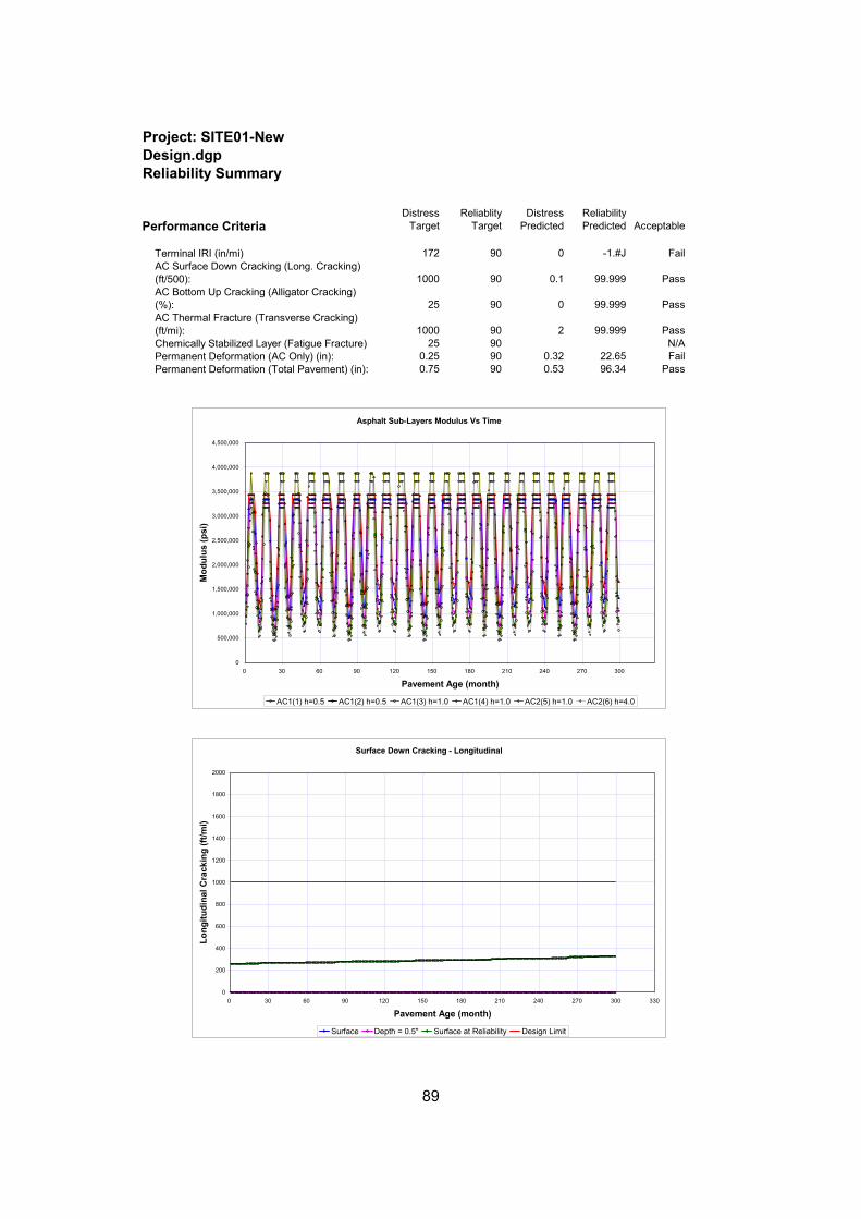
89
Asphalt Sub-Layers Modulus Vs Time
0
500,000
1,000,000
1,500,000
2,000,000
2,500,000
3,000,000
3,500,000
4,000,000
4,500,000
0 30 60 90 120 150 180 210 240 270 300
Pavement Age (month)
Mod
ulus
(psi
)
AC1(1) h=0.5 AC1(2) h=0.5 AC1(3) h=1.0 AC1(4) h=1.0 AC2(5) h=1.0 AC2(6) h=4.0
Surface Down Cracking - Longitudinal
0
200
400
600
800
1000
1200
1400
1600
1800
2000
0 30 60 90 120 150 180 210 240 270 300 330
Pavement Age (month)
Long
itudi
nal C
rack
ing
(ft/m
i)
Surface Depth = 0.5" Surface at Reliability Design Limit
Distress Target
Reliablity Target
Distress Predicted
Reliability Predicted Acceptable
172 90 0 -1.#J Fail
1000 90 0.1 99.999 Pass
25 90 0 99.999 Pass
1000 90 2 99.999 Pass25 90 N/A
0.25 90 0.32 22.65 Fail0.75 90 0.53 96.34 Pass
Project: SITE01-New Design.dgpReliability Summary
Performance Criteria
Terminal IRI (in/mi)
Permanent Deformation (AC Only) (in):Permanent Deformation (Total Pavement) (in):
AC Surface Down Cracking (Long. Cracking) (ft/500):AC Bottom Up Cracking (Alligator Cracking) (%):AC Thermal Fracture (Transverse Cracking) (ft/mi):Chemically Stabilized Layer (Fatigue Fracture)

90
Bottom Up Cracking - Alligator
0
10
20
30
40
50
60
70
80
90
100
0 30 60 90 120 150 180 210 240 270 300 330
Pavement Age (month)
Alli
gato
r Cra
ckin
g (%
)
Maximum Cracking Bottom Up Reliability Maximum Cracking Limit
Thermal Cracking: Total Length Vs Time
0
200
400
600
800
1000
1200
1400
1600
1800
2000
0 30 60 90 120 150 180 210 240 270 300 330
Pavement Age (month)
Tota
l Len
gth
(ft/m
i)
Thermal Crack Length Crack Length at Reliability Design Limit
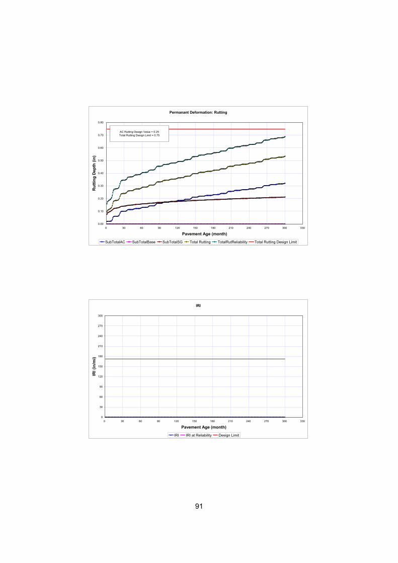
91
Permanant Deformation: Rutting
0.00
0.10
0.20
0.30
0.40
0.50
0.60
0.70
0.80
0 30 60 90 120 150 180 210 240 270 300 330
Pavement Age (month)
Rut
ting
Dep
th (i
n)
SubTotalAC SubTotalBase SubTotalSG Total Rutting TotalRutReliability Total Rutting Design Limit
AC Rutting Design Value = 0.25Total Rutting Design Limit = 0.75
IRI
0
30
60
90
120
150
180
210
240
270
300
0 30 60 90 120 150 180 210 240 270 300 330
Pavement Age (month)
IRI (
in/m
i)
IRI IRI at Reliability Design Limit
92
Limit Reliability63
172 901000 90
25 901000 90
25 900.25 900.75 90
14292
508060
Class 4 Class 5 Class 6 Class 7 Class 8 Class 9 Class 10 Class 11 Class 12 Class 131.00 1.00 1.00 1.00 1.00 1.00 1.00 1.00 1.00 1.00 1.00 1.00 1.00 1.00 1.00 1.00 1.00 1.00 1.00 1.00 1.00 1.00 1.00 1.00 1.00 1.00 1.00 1.00 1.00 1.00 1.00 1.00 1.00 1.00 1.00 1.00 1.00 1.00 1.00 1.00 1.00 1.00 1.00 1.00 1.00 1.00 1.00 1.00 1.00 1.00 1.00 1.00 1.00 1.00 1.00 1.00 1.00 1.00 1.00 1.00 1.00 1.00 1.00 1.00 1.00 1.00 1.00 1.00 1.00 1.00 1.00 1.00 1.00 1.00 1.00 1.00 1.00 1.00 1.00 1.00 1.00 1.00 1.00 1.00 1.00 1.00 1.00 1.00 1.00 1.00 1.00 1.00 1.00 1.00 1.00 1.00 1.00 1.00 1.00 1.00 1.00 1.00 1.00 1.00 1.00 1.00 1.00 1.00 1.00 1.00 1.00 1.00 1.00 1.00 1.00 1.00 1.00 1.00 1.00 1.00
Midnight 2.3% Noon 5.9%1.3% 1:00 am 2.3% 1:00 pm 5.9%8.5% 2:00 am 2.3% 2:00 pm 5.9%2.8% 3:00 am 2.3% 3:00 pm 5.9%0.3% 4:00 am 2.3% 4:00 pm 4.6%7.6% 5:00 am 2.3% 5:00 pm 4.6%
74.0% 6:00 am 5.0% 6:00 pm 4.6%1.2% 7:00 am 5.0% 7:00 pm 4.6%3.4% 8:00 am 5.0% 8:00 pm 3.1%0.6% 9:00 am 5.0% 9:00 pm 3.1%
Project: SITE01-Rehabilitation.dgp
General Information Description:o Route: 29 South o County: Amherst (number 5) o Length: 2640 ft o Number of lanes in each direction: 2 o Pavement Category: Flexible, 10-15 years o Traffic: TT 1,100, AADT 20,000 (one way traffic) o AC overlay 1.5in ; HMA 8in; CTA 6in o Subgrade: wet red, brown, gray sandy silt w/mica, fill material
Design Life 20 yearsExisting pavement construction: September, 1970Pavement overlay construction: September, 1993Traffic open: October, 1993Type of design Flexible
Analysis ParametersAnalysis type Probabilistic
Performance CriteriaInitial IRI (in/mi)Terminal IRI (in/mi)AC Surface Down Cracking (Long. Cracking) (ft/500):AC Bottom Up Cracking (Alligator Cracking) (%):AC Thermal Fracture (Transverse Cracking) (ft/mi):Chemically Stabilized Layer (Fatigue Fracture)Permanent Deformation (AC Only) (in):Permanent Deformation (Total Pavement) (in):
Location: SITE 01Project ID: SITE O1Section ID:
Principal Arterials - Interstate and Defense RoutesDate: 2/13/2005
Station/milepost format: Miles: 0.000Station/milepost begin: 7.8Station/milepost end: 7.3Traffic direction: South bound
Default Input LevelDefault input level Level 3, Default and historical agency values.
Traffic Initial two-way aadtt:Number of lanes in design direction:Percent of trucks in design direction (%):Percent of trucks in design lane (%):Operational speed (mph):
Traffic -- Volume Adjustment FactorsMonthly Adjustment Factors (Level 3, Default MAF)
Vehicle ClassMonth
JanuaryFebruaryMarchAprilMayJuneJulyAugustSeptemberOctoberNovemberDecember
Vehicle Class Distribution Hourly truck traffic distribution(Level 3, Default Distribution) by period beginning:
AADTT distribution by vehicle classClass 4Class 5Class 6Class 7Class 8Class 9Class 10Class 11Class 12

93
4.0%4.0%4.0%4.0%4.0%4.0%4.0%4.0%4.0%4.0%
18
1012
1.62 0.39 0.00 0.00 2.00 0.00 0.00 0.00 1.02 0.99 0.00 0.00 1.00 0.26 0.83 0.00 2.38 0.67 0.00 0.00 1.13 1.93 0.00 0.00 1.19 1.09 0.89 0.00 4.29 0.26 0.06 0.00 3.52 1.14 0.06 0.00 2.15 2.13 0.35 0.00
8.5
12
120120
51.649.249.2
37.57-79.0662823
Traffic Growth Factor
Vehicle Class
Growth Rate
GrowthFunction
Class 4 CompoundClass 5 CompoundClass 6 CompoundClass 7 CompoundClass 8 CompoundClass 9 CompoundClass 10 CompoundClass 11 CompoundClass 12 CompoundClass 13 Compound
Traffic -- Axle Load Distribution FactorsLevel 3: Default
Traffic -- General Traffic InputsMean wheel location (inches from the lane marking):Traffic wander standard deviation (in):Design lane width (ft):
Number of Axles per Truck
Quad Axle
Class 4Class 5Class 6
Vehicle Class
Single Axle
Tandem Axle
Tridem Axle
Class 7Class 8Class 9Class 10Class 11Class 12Class 13
Axle ConfigurationAverage axle width (edge-to-edge) outside dimensions,ft):Dual tire spacing (in):
Axle ConfigurationSingle Tire (psi):Dual Tire (psi):
Average Axle SpacingTandem axle(psi):Tridem axle(psi):Quad axle(psi):
Climate icm file:
site01-02test3Latitude (degrees.minutes)Longitude (degrees.minutes)Elevation (ft)Depth of water table (ft)
Structure--Design Features
Structure--Layers Layer 1 -- Asphalt concrete
Material type: Asphalt concreteLayer thickness (in): 1.5
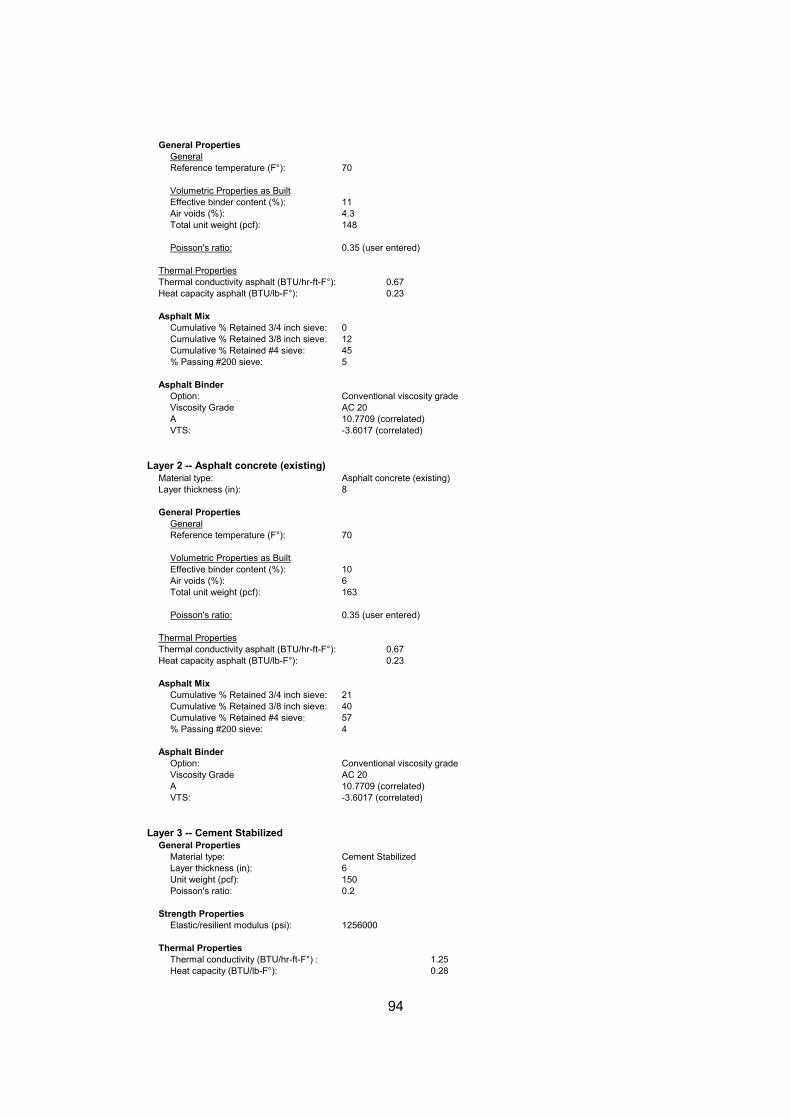
94
General PropertiesGeneralReference temperature (F°): 70
Volumetric Properties as BuiltEffective binder content (%): 11Air voids (%): 4.3Total unit weight (pcf): 148
Poisson's ratio: 0.35 (user entered)
Thermal PropertiesThermal conductivity asphalt (BTU/hr-ft-F°): 0.67Heat capacity asphalt (BTU/lb-F°): 0.23
Asphalt MixCumulative % Retained 3/4 inch sieve: 0Cumulative % Retained 3/8 inch sieve: 12Cumulative % Retained #4 sieve: 45% Passing #200 sieve: 5
Asphalt BinderOption: Conventional viscosity gradeViscosity Grade AC 20A 10.7709 (correlated)VTS: -3.6017 (correlated)
Layer 2 -- Asphalt concrete (existing)Material type: Asphalt concrete (existing)Layer thickness (in): 8
General PropertiesGeneralReference temperature (F°): 70
Volumetric Properties as BuiltEffective binder content (%): 10Air voids (%): 6Total unit weight (pcf): 163
Poisson's ratio: 0.35 (user entered)
Thermal PropertiesThermal conductivity asphalt (BTU/hr-ft-F°): 0.67Heat capacity asphalt (BTU/lb-F°): 0.23
Asphalt MixCumulative % Retained 3/4 inch sieve: 21Cumulative % Retained 3/8 inch sieve: 40Cumulative % Retained #4 sieve: 57% Passing #200 sieve: 4
Asphalt BinderOption: Conventional viscosity gradeViscosity Grade AC 20A 10.7709 (correlated)VTS: -3.6017 (correlated)
Layer 3 -- Cement StabilizedGeneral Properties
Material type: Cement StabilizedLayer thickness (in): 6Unit weight (pcf): 150Poisson's ratio: 0.2
Strength PropertiesElastic/resilient modulus (psi): 1256000
Thermal PropertiesThermal conductivity (BTU/hr-ft-F°) : 1.25Heat capacity (BTU/lb-F°): 0.28
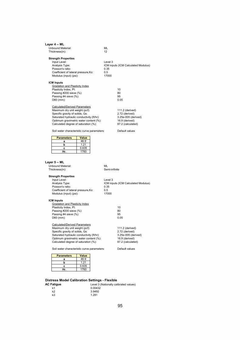
95
Value46.91.21
0.6351760
Value46.91.21
0.6351760
0.004323.94921.281
Layer 4 -- MLUnbound Material: MLThickness(in): 12
Strength PropertiesInput Level: Level 3Analysis Type: ICM inputs (ICM Calculated Modulus)Poisson's ratio: 0.35Coefficient of lateral pressure,Ko: 0.5Modulus (input) (psi): 17000
ICM InputsGradation and Plasticity IndexPlasticity Index, PI: 10Passing #200 sieve (%): 80Passing #4 sieve (%): 95D60 (mm): 0.05
Calculated/Derived ParametersMaximum dry unit weight (pcf): 111.2 (derived)Specific gravity of solids, Gs: 2.72 (derived)Saturated hydraulic conductivity (ft/hr): 3.25e-005 (derived)Optimum gravimetric water content (%): 16.9 (derived)Calculated degree of saturation (%): 87.2 (calculated)
Soil water characteristic curve parameters: Default values
Parametersabc
Hr.
Layer 5 -- MLUnbound Material: MLThickness(in): Semi-infinite
Strength PropertiesInput Level: Level 3Analysis Type: ICM inputs (ICM Calculated Modulus)Poisson's ratio: 0.35Coefficient of lateral pressure,Ko: 0.5Modulus (input) (psi): 17000
ICM InputsGradation and Plasticity IndexPlasticity Index, PI: 10Passing #200 sieve (%): 80Passing #4 sieve (%): 95D60 (mm): 0.05
Calculated/Derived ParametersMaximum dry unit weight (pcf): 111.2 (derived)Specific gravity of solids, Gs: 2.72 (derived)Saturated hydraulic conductivity (ft/hr): 3.25e-005 (derived)Optimum gravimetric water content (%): 16.9 (derived)Calculated degree of saturation (%): 87.2 (calculated)
Soil water characteristic curve parameters: Default values
Parametersabc
Hr.
Distress Model Calibration Settings - Flexible AC Fatigue Level 3 (Nationally calibrated values)
k1k2k3

96
-3.44881.56060.4791
5
11
1.673
1.35
73.501000
1106000
1101000
0.0115050.0035993.4300570.0007230.0112419.042440.179
0.0082630.0221831.330410.197
AC Rutting Level 3 (Nationally calibrated values)k1k2k3
Standard Deviation Total Rutting (RUT):
0.1587*POWER(RUT,0.4579)+0.001
Thermal Fracture Level 3 (Nationally calibrated values)k1
Std. Dev. (THERMAL): 0.2474 * THERMAL + 10.619
CSM Fatigue Level 3 (Nationally calibrated values)k1k2
Subgrade Rutting Level 3 (Nationally calibrated values)Granular:
k1Fine-grain:
k1
AC CrackingAC Top Down Cracking
C1 (top)C2 (top)C3 (top)C4 (top)
Standard Deviation (TOP) 200 + 2300/(1+exp(1.072-2.1654*log(TOP+0.0001)))
AC Bottom Up CrackingC1 (bottom)C2 (bottom)C3 (bottom)C4 (bottom)
Standard Deviation (TOP) 32.7 + 995.1 /(1+exp(2-2*log(BOTTOM+0.001)))
CSM CrackingC1 (CSM)C2 (CSM)C3 (CSM)C4 (CSM)
Standard Deviation (CSM) CTB*11
IRIIRI Rehabilitation over Flexible
C1 (Flexible)C2 (Flexible)C3 (Flexible)C4 (Flexible)C5 (Flexible)C6 (Flexible)
C3 (Rigid)Std. Dev (Rigid)
Std. Dev (Flexible)
IRI Rehabilitation over RigidC1 (Rigid)C2 (Rigid)

97
Asphalt Sub-Layers Modulus Vs Time
0
500,000
1,000,000
1,500,000
2,000,000
2,500,000
3,000,000
3,500,000
4,000,000
0 24 48 72 96 120 144 168 192 216 240
Pavement Age (month)
Mod
ulus
(psi
)
AC1(1) h=0.5 AC1(2) h=1.0 AC2(3) h=1.0 AC2(4) h=1.0 AC2(5) h=1.0 AC2(6) h=5.0
Surface Down Cracking - Longitudinal
0
200
400
600
800
1000
1200
1400
1600
1800
2000
0 24 48 72 96 120 144 168 192 216 240 264
Pavement Age (month)
Long
itudi
nal C
rack
ing
(ft/m
i)
Surface Depth = 0.5" Surface at Reliability Design Limit
Distress Target
Reliablity Target
Distress Predicted
Reliability Predicted Acceptable
172 90 245.1 11.24 Fail
1000 90 1.3 99.31 Pass
25 90 0 99.999 Pass
1000 90 485 99.999 Pass25 90 N/A
0.25 90 0.42 5.5 Fail0.75 90 0.58 91.29 Pass
Project: SITE01-Rehabilitation.dgpReliability Summary
Performance Criteria
Terminal IRI (in/mi)
Permanent Deformation (AC Only) (in):Permanent Deformation (Total Pavement) (in):
AC Surface Down Cracking (Long. Cracking) (ft/500):AC Bottom Up Cracking (Alligator Cracking) (%):AC Thermal Fracture (Transverse Cracking) (ft/mi):Chemically Stabilized Layer (Fatigue Fracture)

98
Bottom Up Cracking - Alligator
0
10
20
30
40
50
60
70
80
90
100
0 24 48 72 96 120 144 168 192 216 240 264
Pavement Age (month)
Alli
gato
r Cra
ckin
g (%
)
Maximum Cracking Bottom Up Reliability Maximum Cracking Limit
Thermal Cracking: Total Length Vs Time
0
200
400
600
800
1000
1200
1400
1600
1800
2000
0 24 48 72 96 120 144 168 192 216 240 264
Pavement Age (month)
Tota
l Len
gth
(ft/m
i)
Thermal Crack Length Crack Length at Reliability Design Limit

99
Permanant Deformation: Rutting
0.00
0.10
0.20
0.30
0.40
0.50
0.60
0.70
0.80
0 24 48 72 96 120 144 168 192 216 240 264
Pavement Age (month)
Rut
ting
Dep
th (i
n)
SubTotalAC SubTotalBase SubTotalSGTotal Rutting TotalRutReliability Total Rutting Design Limit
AC Rutting Design Value = 0.25Total Rutting Design Limit = 0.75
IRI
0
30
60
90
120
150
180
210
240
270
300
0 24 48 72 96 120 144 168 192 216 240 264
Pavement Age (month)
IRI (
in/m
i)
IRI IRI at Reliability Design Limit

100
Limit Reliability63
172 901000 90
25 901000 90
25 900.25 900.75 90
18542
508060
Class 4 Class 5 Class 6 Class 7 Class 8 Class 9 Class 10 Class 11 Class 12 Class 131.00 1.00 1.00 1.00 1.00 1.00 1.00 1.00 1.00 1.00 1.00 1.00 1.00 1.00 1.00 1.00 1.00 1.00 1.00 1.00 1.00 1.00 1.00 1.00 1.00 1.00 1.00 1.00 1.00 1.00 1.00 1.00 1.00 1.00 1.00 1.00 1.00 1.00 1.00 1.00 1.00 1.00 1.00 1.00 1.00 1.00 1.00 1.00 1.00 1.00 1.00 1.00 1.00 1.00 1.00 1.00 1.00 1.00 1.00 1.00 1.00 1.00 1.00 1.00 1.00 1.00 1.00 1.00 1.00 1.00 1.00 1.00 1.00 1.00 1.00 1.00 1.00 1.00 1.00 1.00 1.00 1.00 1.00 1.00 1.00 1.00 1.00 1.00 1.00 1.00 1.00 1.00 1.00 1.00 1.00 1.00 1.00 1.00 1.00 1.00 1.00 1.00 1.00 1.00 1.00 1.00 1.00 1.00 1.00 1.00 1.00 1.00 1.00 1.00 1.00 1.00 1.00 1.00 1.00 1.00
Midnight 2.3% Noon 5.9%1.3% 1:00 am 2.3% 1:00 pm 5.9%8.5% 2:00 am 2.3% 2:00 pm 5.9%2.8% 3:00 am 2.3% 3:00 pm 5.9%0.3% 4:00 am 2.3% 4:00 pm 4.6%7.6% 5:00 am 2.3% 5:00 pm 4.6%
74.0% 6:00 am 5.0% 6:00 pm 4.6%1.2% 7:00 am 5.0% 7:00 pm 4.6%3.4% 8:00 am 5.0% 8:00 pm 3.1%0.6% 9:00 am 5.0% 9:00 pm 3.1%0.3% 10:00 am 5.9% 10:00 pm 3.1%
11:00 am 5.9% 11:00 pm 3.1%
Project: SITE16-New Design.dgp
General Information Description:o Route: 81 North o County: Frederick, Winchester (number 34) o Length: 2640 ft o Number of lanes in each direction: 2 o Pavement Category: Flexible, older than 20 years w/surface older than 10 years o AC overlay 1.8in HMA:9.7in Agg Base+Select Mat'l: 18in o Subgrade: B1: clay w/silts (10%) and gray compacted clay with gravel/sand (fill) B2: damp clay w/silts (10%)
Design Life 15 yearsBase/Subgrade construction: August, 1965Pavement construction: September, 1965Traffic open: October, 1965Type of design Flexible
Analysis ParametersAnalysis type Probabilistic
Performance CriteriaInitial IRI (in/mi)Terminal IRI (in/mi)AC Surface Down Cracking (Long. Cracking) (ft/500):AC Bottom Up Cracking (Alligator Cracking) (%):AC Thermal Fracture (Transverse Cracking) (ft/mi):Chemically Stabilized Layer (Fatigue Fracture)Permanent Deformation (AC Only) (in):Permanent Deformation (Total Pavement) (in):
Location: SITE 16Project ID: SITE 16Section ID:
Principal Arterials - Interstate and Defense RoutesDate: 2/13/2005
Station/milepost format: Miles: 0.000Station/milepost begin: 21.37Station/milepost end: 21.87Traffic direction: North bound
Default Input LevelDefault input level Level 3, Default and historical agency values.
Traffic Initial two-way aadtt:Number of lanes in design direction:Percent of trucks in design direction (%):Percent of trucks in design lane (%):Operational speed (mph):
Traffic -- Volume Adjustment FactorsMonthly Adjustment Factors (Level 3, Default MAF)
Vehicle ClassMonth
JanuaryFebruaryMarchAprilMayJuneJulyAugustSeptemberOctoberNovemberDecember
Vehicle Class Distribution Hourly truck traffic distribution(Level 3, Default Distribution) by period beginning:
AADTT distribution by vehicle classClass 4Class 5Class 6Class 7Class 8Class 9Class 10Class 11Class 12Class 13

101
4.0%4.0%4.0%4.0%4.0%4.0%4.0%4.0%4.0%4.0%
18
1012
1.62 0.39 0.00 0.00 2.00 0.00 0.00 0.00 1.02 0.99 0.00 0.00 1.00 0.26 0.83 0.00 2.38 0.67 0.00 0.00 1.13 1.93 0.00 0.00 1.19 1.09 0.89 0.00 4.29 0.26 0.06 0.00 3.52 1.14 0.06 0.00 2.15 2.13 0.35 0.00
8.5
12
120120
51.649.249.2
36.26-77.4324815
Traffic Growth Factor
Vehicle Class
Growth Rate
GrowthFunction
Class 4 CompoundClass 5 CompoundClass 6 CompoundClass 7 CompoundClass 8 CompoundClass 9 CompoundClass 10 CompoundClass 11 CompoundClass 12 CompoundClass 13 Compound
Traffic -- Axle Load Distribution FactorsLevel 3: Default
Traffic -- General Traffic InputsMean wheel location (inches from the lane marking):Traffic wander standard deviation (in):Design lane width (ft):
Number of Axles per Truck
Quad Axle
Class 4Class 5Class 6
Vehicle Class
Single Axle
Tandem Axle
Tridem Axle
Class 7Class 8Class 9Class 10Class 11Class 12Class 13
Axle ConfigurationAverage axle width (edge-to-edge) outside dimensions,ft):Dual tire spacing (in):
Axle ConfigurationSingle Tire (psi):Dual Tire (psi):
Average Axle SpacingTandem axle(psi):Tridem axle(psi):Quad axle(psi):
Climate icm file:
site16-01DLatitude (degrees.minutes)Longitude (degrees.minutes)Elevation (ft)Depth of water table (ft)
Structure--Design Features
Structure--Layers Layer 1 -- Asphalt concrete
Material type: Asphalt concreteLayer thickness (in): 1.8

102
General PropertiesGeneralReference temperature (F°): 70
Volumetric Properties as BuiltEffective binder content (%): 11Air voids (%): 4.5Total unit weight (pcf): 145
Poisson's ratio: 0.35 (user entered)
Thermal PropertiesThermal conductivity asphalt (BTU/hr-ft-F°): 0.67Heat capacity asphalt (BTU/lb-F°): 0.23
Asphalt MixCumulative % Retained 3/4 inch sieve: 0Cumulative % Retained 3/8 inch sieve: 12Cumulative % Retained #4 sieve: 45% Passing #200 sieve: 5
Asphalt BinderOption: Conventional viscosity gradeViscosity Grade AC 30A 10.6316 (correlated)VTS: -3.548 (correlated)
Layer 2 -- Asphalt concreteMaterial type: Asphalt concreteLayer thickness (in): 7.9
General PropertiesGeneralReference temperature (F°): 70
Volumetric Properties as BuiltEffective binder content (%): 10Air voids (%): 6Total unit weight (pcf): 163
Poisson's ratio: 0.35 (user entered)
Thermal PropertiesThermal conductivity asphalt (BTU/hr-ft-F°): 0.67Heat capacity asphalt (BTU/lb-F°): 0.23
Asphalt MixCumulative % Retained 3/4 inch sieve: 21Cumulative % Retained 3/8 inch sieve: 40Cumulative % Retained #4 sieve: 57% Passing #200 sieve: 4
Asphalt BinderOption: Conventional viscosity gradeViscosity Grade AC 20A 10.7709 (correlated)VTS: -3.6017 (correlated)
Layer 3 -- Crushed stoneUnbound Material: Crushed stoneThickness(in): 18
Strength PropertiesInput Level: Level 3Analysis Type: ICM inputs (ICM Calculated Modulus)Poisson's ratio: 0.35Coefficient of lateral pressure,Ko: 0.5Modulus (input) (psi): 90000

103
Value11.41.720.518371
Value68.11.150.6582720
0.004323.94921.281
-3.44881.56060.4791
5
ICM InputsGradation and Plasticity IndexPlasticity Index, PI: 1Passing #200 sieve (%): 10Passing #4 sieve (%): 54D60 (mm): 9
Calculated/Derived ParametersMaximum dry unit weight (pcf): 122.3 (derived)Specific gravity of solids, Gs: 2.67 (derived)Saturated hydraulic conductivity (ft/hr): 285 (derived)Optimum gravimetric water content (%): 11.2 (derived)Calculated degree of saturation (%): 82.8 (calculated)
Soil water characteristic curve parameters: Default values
Parametersabc
Hr.
Layer 4 -- CLUnbound Material: CLThickness(in): Semi-infinite
Strength PropertiesInput Level: Level 3Analysis Type: ICM inputs (ICM Calculated Modulus)Poisson's ratio: 0.35Coefficient of lateral pressure,Ko: 0.5Modulus (input) (psi): 36000
ICM InputsGradation and Plasticity IndexPlasticity Index, PI: 15Passing #200 sieve (%): 75Passing #4 sieve (%): 95D60 (mm): 0.1
Calculated/Derived ParametersMaximum dry unit weight (pcf): 107.9 (derived)Specific gravity of solids, Gs: 2.73 (derived)Saturated hydraulic conductivity (ft/hr): 3.25e-005 (derived)Optimum gravimetric water content (%): 18.6 (derived)Calculated degree of saturation (%): 87.6 (calculated)
Soil water characteristic curve parameters: Default values
Parametersabc
Hr.
Distress Model Calibration Settings - Flexible AC Fatigue Level 3 (Nationally calibrated values)
k1k2k3
AC Rutting Level 3 (Nationally calibrated values)k1k2k3
Standard Deviation Total Rutting (RUT):
0.1587*POWER(RUT,0.4579)+0.001
Thermal Fracture Level 3 (Nationally calibrated values)k1

104
11
1.673
1.35
73.501000
1106000
1101000
0.04630.001190.18340.003840.007360.001150.387
0.0099950.0005180.0023518.360.96940.292
0.007320.076470.0001450.008420.0002120.229
CSM Fatigue Level 3 (Nationally calibrated values)k1k2
Subgrade Rutting Level 3 (Nationally calibrated values)Granular:
k1Fine-grain:
k1
AC CrackingAC Top Down Cracking
C1 (top)C2 (top)C3 (top)C4 (top)
Standard Deviation (TOP) 200 + 2300/(1+exp(1.072-2.1654*log(TOP+0.0001)))
AC Bottom Up CrackingC1 (bottom)C2 (bottom)C3 (bottom)C4 (bottom)
Standard Deviation (TOP) 32.7 + 995.1 /(1+exp(2-2*log(BOTTOM+0.0001)))
CSM CrackingC1 (CSM)C2 (CSM)C3 (CSM)C4 (CSM)
Standard Deviation (CSM) CTB*1
IRIIRI Flexible Pavements with GB
C1 (GB)C2 (GB)C3 (GB)C4 (GB)C5 (GB)C6 (GB)Std. Dev (GB)
IRI Flexible Pavements with ATBC1 (ATB)C2 (ATB)C3 (ATB)C4 (ATB)C5 (ATB)Std. Dev (ATB)
IRI Flexible Pavements with CSMC1 (CSM)
Std. Dev (CSM)
C2 (CSM)C3 (CSM)C4 (CSM)C5 (CSM)

105
Distress Target
Reliablity Target
Distress Predicted
Reliability Predicted Acceptable
172 90 111.1 99.29 Pass
1000 90 1.8 98.67 Pass
25 90 0.1 99.999 Pass
1000 90 1 99.999 Pass25 90 N/A
0.25 90 0.35 15.61 Fail0.75 90 0.44 99.8 Pass
Project: SITE16-New Design.dgpReliability Summary
Performance Criteria
Terminal IRI (in/mi)
Permanent Deformation (AC Only) (in):Permanent Deformation (Total Pavement) (in):
AC Surface Down Cracking (Long. Cracking) (ft/500):AC Bottom Up Cracking (Alligator Cracking) (%):AC Thermal Fracture (Transverse Cracking) (ft/mi):Chemically Stabilized Layer (Fatigue Fracture)
Asphalt Sub-Layers Modulus Vs Time
0
500,000
1,000,000
1,500,000
2,000,000
2,500,000
3,000,000
3,500,000
4,000,000
4,500,000
0 18 36 54 72 90 108 126 144 162 180
Pavement Age (month)
Mod
ulus
(psi
)
AC1(1) h=0.5 AC1(2) h=1.3 AC2(3) h=1.0 AC2(4) h=1.0 AC2(5) h=1.0 AC2(6) h=4.9
Surface Down Cracking - Longitudinal
0
200
400
600
800
1000
1200
1400
1600
1800
2000
0 18 36 54 72 90 108 126 144 162 180 198
Pavement Age (month)
Long
itudi
nal C
rack
ing
(ft/m
i)
Surface Depth = 0.5" Surface at Reliability Design Limit

106
Bottom Up Cracking - Alligator
0
10
20
30
40
50
60
70
80
90
100
0 18 36 54 72 90 108 126 144 162 180 198
Pavement Age (month)
Alli
gato
r Cra
ckin
g (%
)
Maximum Cracking Bottom Up Reliability Maximum Cracking Limit
Thermal Cracking: Total Length Vs Time
0
200
400
600
800
1000
1200
1400
1600
1800
2000
0 18 36 54 72 90 108 126 144 162 180 198
Pavement Age (month)
Tota
l Len
gth
(ft/m
i)
Thermal Crack Length Crack Length at Reliability Design Limit

107
Permanant Deformation: Rutting
0.00
0.10
0.20
0.30
0.40
0.50
0.60
0.70
0.80
0 18 36 54 72 90 108 126 144 162 180 198
Pavement Age (month)
Rut
ting
Dep
th (i
n)
SubTotalAC SubTotalBase SubTotalSGTotal Rutting TotalRutReliability Total Rutting Design Limit
AC Rutting Design Value = 0.25Total Rutting Design Limit = 0.75
IRI
0
20
40
60
80
100
120
140
160
180
200
0 18 36 54 72 90 108 126 144 162 180 198
Pavement Age (month)
IRI (
in/m
i)
IRI IRI at Reliability Design Limit

108
Limit Reliability63
172 901000 90
25 901000 90
25 900.25 900.75 90
51412
508060
Class 4 Class 5 Class 6 Class 7 Class 8 Class 9 Class 10 Class 11 Class 12 Class 131.00 1.00 1.00 1.00 1.00 1.00 1.00 1.00 1.00 1.00 1.00 1.00 1.00 1.00 1.00 1.00 1.00 1.00 1.00 1.00 1.00 1.00 1.00 1.00 1.00 1.00 1.00 1.00 1.00 1.00 1.00 1.00 1.00 1.00 1.00 1.00 1.00 1.00 1.00 1.00 1.00 1.00 1.00 1.00 1.00 1.00 1.00 1.00 1.00 1.00 1.00 1.00 1.00 1.00 1.00 1.00 1.00 1.00 1.00 1.00 1.00 1.00 1.00 1.00 1.00 1.00 1.00 1.00 1.00 1.00 1.00 1.00 1.00 1.00 1.00 1.00 1.00 1.00 1.00 1.00 1.00 1.00 1.00 1.00 1.00 1.00 1.00 1.00 1.00 1.00 1.00 1.00 1.00 1.00 1.00 1.00 1.00 1.00 1.00 1.00 1.00 1.00 1.00 1.00 1.00 1.00 1.00 1.00 1.00 1.00 1.00 1.00 1.00 1.00 1.00 1.00 1.00 1.00 1.00 1.00
Midnight 2.3% Noon 5.9%1.3% 1:00 am 2.3% 1:00 pm 5.9%8.5% 2:00 am 2.3% 2:00 pm 5.9%2.8% 3:00 am 2.3% 3:00 pm 5.9%0.3% 4:00 am 2.3% 4:00 pm 4.6%7.6% 5:00 am 2.3% 5:00 pm 4.6%
74.0% 6:00 am 5.0% 6:00 pm 4.6%1.2% 7:00 am 5.0% 7:00 pm 4.6%3.4% 8:00 am 5.0% 8:00 pm 3.1%0.6% 9:00 am 5.0% 9:00 pm 3.1%
Project: SITE16 - Rehabilitation.dgp
General Information Description:o Route: 81 North o County: Frederick, Winchester (number 34) o Length: 2640 ft o Number of lanes in each direction: 2 o Pavement Category: Flexible, older than 20 years w/surface older than 10 years o AC overlay 1.8in HMA:9.7in Agg Base+Select Mat'l: 18in o Subgrade: B1: clay w/silts (10%) and gray compacted clay with gravel/sand (fill) B2: damp clay w/silts (10%)
Design Life 20 yearsExisting pavement construction: September, 1965Pavement overlay construction: September, 1991Traffic open: September, 1991Type of design Flexible
Analysis ParametersAnalysis type Probabilistic
Performance CriteriaInitial IRI (in/mi)Terminal IRI (in/mi)AC Surface Down Cracking (Long. Cracking) (ft/500):AC Bottom Up Cracking (Alligator Cracking) (%):AC Thermal Fracture (Transverse Cracking) (ft/mi):Chemically Stabilized Layer (Fatigue Fracture)Permanent Deformation (AC Only) (in):Permanent Deformation (Total Pavement) (in):
Location: SITE 16Project ID: SITE 16Section ID:
Principal Arterials - Interstate and Defense RoutesDate: 2/13/2005
Station/milepost format: Miles: 0.000Station/milepost begin: 21.37Station/milepost end: 21.87Traffic direction: North bound
Default Input LevelDefault input level Level 3, Default and historical agency values.
Traffic Initial two-way aadtt:Number of lanes in design direction:Percent of trucks in design direction (%):Percent of trucks in design lane (%):Operational speed (mph):
Traffic -- Volume Adjustment FactorsMonthly Adjustment Factors (Level 3, Default MAF)
Vehicle ClassMonth
JanuaryFebruaryMarchAprilMayJuneJulyAugustSeptemberOctoberNovemberDecember
Vehicle Class Distribution Hourly truck traffic distribution(Level 3, Default Distribution) by period beginning:
AADTT distribution by vehicle classClass 4Class 5Class 6Class 7Class 8Class 9Class 10Class 11Class 12
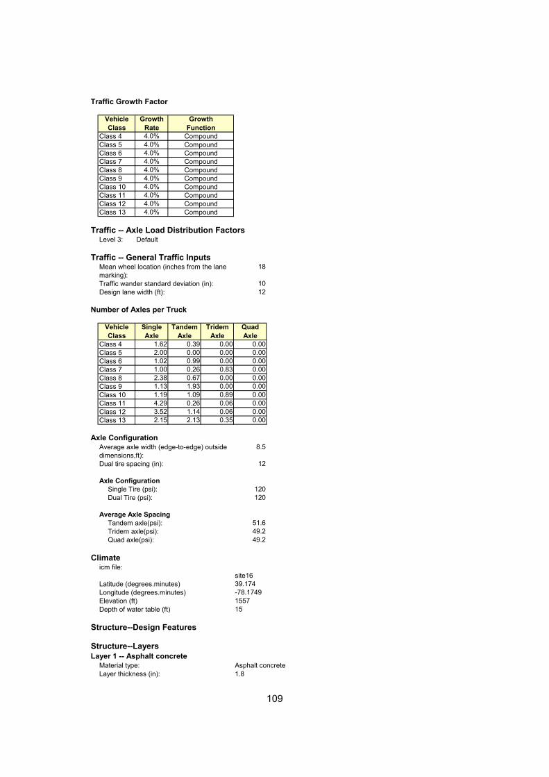
109
4.0%4.0%4.0%4.0%4.0%4.0%4.0%4.0%4.0%4.0%
18
1012
1.62 0.39 0.00 0.00 2.00 0.00 0.00 0.00 1.02 0.99 0.00 0.00 1.00 0.26 0.83 0.00 2.38 0.67 0.00 0.00 1.13 1.93 0.00 0.00 1.19 1.09 0.89 0.00 4.29 0.26 0.06 0.00 3.52 1.14 0.06 0.00 2.15 2.13 0.35 0.00
8.5
12
120120
51.649.249.2
39.174-78.1749155715
Traffic Growth Factor
Vehicle Class
Growth Rate
GrowthFunction
Class 4 CompoundClass 5 CompoundClass 6 CompoundClass 7 CompoundClass 8 CompoundClass 9 CompoundClass 10 CompoundClass 11 CompoundClass 12 CompoundClass 13 Compound
Traffic -- Axle Load Distribution FactorsLevel 3: Default
Traffic -- General Traffic InputsMean wheel location (inches from the lane marking):Traffic wander standard deviation (in):Design lane width (ft):
Number of Axles per Truck
Quad Axle
Class 4Class 5Class 6
Vehicle Class
Single Axle
Tandem Axle
Tridem Axle
Class 7Class 8Class 9Class 10Class 11Class 12Class 13
Axle ConfigurationAverage axle width (edge-to-edge) outside dimensions,ft):Dual tire spacing (in):
Axle ConfigurationSingle Tire (psi):Dual Tire (psi):
Average Axle SpacingTandem axle(psi):Tridem axle(psi):Quad axle(psi):
Climate icm file:
site16Latitude (degrees.minutes)Longitude (degrees.minutes)Elevation (ft)Depth of water table (ft)
Structure--Design Features
Structure--Layers Layer 1 -- Asphalt concrete
Material type: Asphalt concreteLayer thickness (in): 1.8

110
General PropertiesGeneralReference temperature (F°): 70
Volumetric Properties as BuiltEffective binder content (%): 11Air voids (%): 4.5Total unit weight (pcf): 148
Poisson's ratio: 0.35 (user entered)
Thermal PropertiesThermal conductivity asphalt (BTU/hr-ft-F°): 0.67Heat capacity asphalt (BTU/lb-F°): 0.23
Asphalt MixCumulative % Retained 3/4 inch sieve: 0Cumulative % Retained 3/8 inch sieve: 12Cumulative % Retained #4 sieve: 45% Passing #200 sieve: 5
Asphalt BinderOption: Conventional viscosity gradeViscosity Grade AC 30A 10.6316 (correlated)VTS: -3.548 (correlated)
Layer 2 -- Asphalt concrete (existing)Material type: Asphalt concrete (existing)Layer thickness (in): 9.7
General PropertiesGeneralReference temperature (F°): 70
Volumetric Properties as BuiltEffective binder content (%): 11Air voids (%): 8.5Total unit weight (pcf): 148
Poisson's ratio: 0.35 (user entered)
Thermal PropertiesThermal conductivity asphalt (BTU/hr-ft-F°): 0.67Heat capacity asphalt (BTU/lb-F°): 0.23
Asphalt MixCumulative % Retained 3/4 inch sieve: 21Cumulative % Retained 3/8 inch sieve: 40Cumulative % Retained #4 sieve: 57% Passing #200 sieve: 4
Asphalt BinderOption: Conventional viscosity gradeViscosity Grade AC 20A 10.7709 (correlated)VTS: -3.6017 (correlated)
Layer 3 -- Crushed stoneUnbound Material: Crushed stoneThickness(in): 18

111
Value11.41.72
0.518371
Value68.11.15
0.6582720
0.004323.94921.281
Strength PropertiesInput Level: Level 3Analysis Type: ICM inputs (ICM Calculated Modulus)Poisson's ratio: 0.35Coefficient of lateral pressure,Ko: 0.5Modulus (input) (psi): 90000
ICM InputsGradation and Plasticity IndexPlasticity Index, PI: 1Passing #200 sieve (%): 10Passing #4 sieve (%): 54D60 (mm): 2
Calculated/Derived ParametersMaximum dry unit weight (pcf): 122.3 (derived)Specific gravity of solids, Gs: 2.67 (derived)Saturated hydraulic conductivity (ft/hr): 37 (derived)Optimum gravimetric water content (%): 11.2 (derived)Calculated degree of saturation (%): 82.8 (calculated)
Soil water characteristic curve parameters: Default values
Parametersabc
Hr.
Layer 4 -- CLUnbound Material: CLThickness(in): Semi-infinite
Strength PropertiesInput Level: Level 3Analysis Type: ICM inputs (ICM Calculated Modulus)Poisson's ratio: 0.35Coefficient of lateral pressure,Ko: 0.5Modulus (input) (psi): 36000
ICM InputsGradation and Plasticity IndexPlasticity Index, PI: 15Passing #200 sieve (%): 75Passing #4 sieve (%): 95D60 (mm): 0.1
Calculated/Derived ParametersMaximum dry unit weight (pcf): 107.9 (derived)Specific gravity of solids, Gs: 2.73 (derived)Saturated hydraulic conductivity (ft/hr): 3.25e-005 (derived)Optimum gravimetric water content (%): 18.6 (derived)Calculated degree of saturation (%): 87.6 (calculated)
Soil water characteristic curve parameters: Default values
Parametersabc
Hr.
Distress Model Calibration Settings - Flexible AC Fatigue Level 3 (Nationally calibrated values)
k1k2k3

112
-3.44881.56060.4791
5
11
1.673
1.35
73.501000
1106000
1101000
0.0115050.0035993.4300570.0007230.0112419.042440.179
0.0082630.0221831.330410.197
AC Rutting Level 3 (Nationally calibrated values)k1k2k3
Standard Deviation Total Rutting (RUT):
0.1587*POWER(RUT,0.4579)+0.001
Thermal Fracture Level 3 (Nationally calibrated values)k1
Std. Dev. (THERMAL): 0.2474 * THERMAL + 10.619
CSM Fatigue Level 3 (Nationally calibrated values)k1k2
Subgrade Rutting Level 3 (Nationally calibrated values)Granular:
k1Fine-grain:
k1
AC CrackingAC Top Down Cracking
C1 (top)C2 (top)C3 (top)C4 (top)
Standard Deviation (TOP) 200 + 2300/(1+exp(1.072-2.1654*log(TOP+0.0001)))
AC Bottom Up CrackingC1 (bottom)C2 (bottom)C3 (bottom)C4 (bottom)
Standard Deviation (TOP) 32.7 + 995.1 /(1+exp(2-2*log(BOTTOM+0.001)))
CSM CrackingC1 (CSM)C2 (CSM)C3 (CSM)C4 (CSM)
Standard Deviation (CSM) CTB*11
IRIIRI Rehabilitation over Flexible
C1 (Flexible)C2 (Flexible)C3 (Flexible)C4 (Flexible)C5 (Flexible)C6 (Flexible)Std. Dev (Flexible)
IRI Rehabilitation over RigidC1 (Rigid)C2 (Rigid)C3 (Rigid)Std. Dev (Rigid)

113
Distress Target
Reliablity Target
Distress Predicted
Reliability Predicted Acceptable
172 90 239.4 13.14 Fail
1000 90 526 59.11 Fail
25 90 0 99.999 Pass
1000 90 1 99.999 Pass25 90 N/A
0.25 90 0.56 0.6 Fail0.75 90 0.65 78.8 Fail
Reliability Summary
Performance Criteria
Terminal IRI (in/mi)
Project: SITE16-Rehabilitation.dgp
Permanent Deformation (AC Only) (in):Permanent Deformation (Total Pavement) (in):
AC Surface Down Cracking (Long. Cracking) (ft/500):AC Bottom Up Cracking (Alligator Cracking) (%):AC Thermal Fracture (Transverse Cracking) (ft/mi):Chemically Stabilized Layer (Fatigue Fracture)
Asphalt Sub-Layers Modulus Vs Time
0
500,000
1,000,000
1,500,000
2,000,000
2,500,000
3,000,000
3,500,000
4,000,000
0 24 48 72 96 120 144 168 192 216 240
Pavement Age (month)
Mod
ulus
(psi
)
AC1(1) h=0.5 AC1(2) h=1.3 AC2(3) h=1.0 AC2(4) h=1.0 AC2(5) h=1.0AC2(6) h=4.0 AC2(7) h=4.7
Surface Down Cracking - Longitudinal
0
400
800
1200
1600
2000
2400
2800
3200
3600
4000
0 24 48 72 96 120 144 168 192 216 240 264
Pavement Age (month)
Long
itudi
nal C
rack
ing
(ft/m
i)
Surface Depth = 0.5" Surface at Reliability Design Limit

114
Bottom Up Cracking - Alligator
0
10
20
30
40
50
60
70
80
90
100
0 24 48 72 96 120 144 168 192 216 240 264
Pavement Age (month)
Alli
gato
r Cra
ckin
g (%
)
Maximum Cracking Bottom Up Reliability Maximum Cracking Limit
Thermal Cracking: Total Length Vs Time
0
200
400
600
800
1000
1200
1400
1600
1800
2000
0 24 48 72 96 120 144 168 192 216 240 264
Pavement Age (month)
Tota
l Len
gth
(ft/m
i)
Thermal Crack Length Crack Length at Reliability Design Limit

115
Permanant Deformation: Rutting
0.00
0.10
0.20
0.30
0.40
0.50
0.60
0.70
0.80
0.90
0 24 48 72 96 120 144 168 192 216 240 264
Pavement Age (month)
Rut
ting
Dep
th (i
n)
SubTotalAC SubTotalBase SubTotalSGTotal Rutting TotalRutReliability Total Rutting Design Limit
AC Rutting Design Value = 0.25Total Rutting Design Limit = 0.75
IRI
0
30
60
90
120
150
180
210
240
270
300
0 24 48 72 96 120 144 168 192 216 240 264
Pavement Age (month)
IRI (
in/m
i)
IRI IRI at Reliability Design Limit

116
Limit Reliability63
172 901000 90
25 901000 90
25 900.25 900.75 90
97643
507560
Class 4 Class 5 Class 6 Class 7 Class 8 Class 9 Class 10 Class 11 Class 12 Class 131.00 1.00 1.00 1.00 1.00 1.00 1.00 1.00 1.00 1.00 1.00 1.00 1.00 1.00 1.00 1.00 1.00 1.00 1.00 1.00 1.00 1.00 1.00 1.00 1.00 1.00 1.00 1.00 1.00 1.00 1.00 1.00 1.00 1.00 1.00 1.00 1.00 1.00 1.00 1.00 1.00 1.00 1.00 1.00 1.00 1.00 1.00 1.00 1.00 1.00 1.00 1.00 1.00 1.00 1.00 1.00 1.00 1.00 1.00 1.00 1.00 1.00 1.00 1.00 1.00 1.00 1.00 1.00 1.00 1.00 1.00 1.00 1.00 1.00 1.00 1.00 1.00 1.00 1.00 1.00 1.00 1.00 1.00 1.00 1.00 1.00 1.00 1.00 1.00 1.00 1.00 1.00 1.00 1.00 1.00 1.00 1.00 1.00 1.00 1.00 1.00 1.00 1.00 1.00 1.00 1.00 1.00 1.00 1.00 1.00 1.00 1.00 1.00 1.00 1.00 1.00 1.00 1.00 1.00 1.00
Midnight 2.3% Noon 5.9%1.3% 1:00 am 2.3% 1:00 pm 5.9%8.5% 2:00 am 2.3% 2:00 pm 5.9%2.8% 3:00 am 2.3% 3:00 pm 5.9%0.3% 4:00 am 2.3% 4:00 pm 4.6%7.6% 5:00 am 2.3% 5:00 pm 4.6%
74.0% 6:00 am 5.0% 6:00 pm 4.6%1.2% 7:00 am 5.0% 7:00 pm 4.6%3.4% 8:00 am 5.0% 8:00 pm 3.1%0.6% 9:00 am 5.0% 9:00 pm 3.1%
Class 9Class 10Class 11Class 12
Class 5Class 6Class 7Class 8
(Level 3, Default Distribution) by period beginning:AADTT distribution by vehicle classClass 4
NovemberDecember
Vehicle Class Distribution Hourly truck traffic distribution
JulyAugustSeptemberOctober
MarchAprilMayJune
Vehicle ClassMonth
JanuaryFebruary
Percent of trucks in design lane (%):Operational speed (mph):
Traffic -- Volume Adjustment FactorsMonthly Adjustment Factors (Level 3, Default MAF)
Traffic Initial two-way aadtt:Number of lanes in design direction:Percent of trucks in design direction (%):
Traffic direction: South bound
Default Input LevelDefault input level Level 3, Default and historical agency values.
Station/milepost begin: 1.5Station/milepost end: 1
Station/milepost format: Miles: 0.000
Principal Arterials - Interstate and Defense RoutesDate: 2/28/2005
Project ID: SITE18Section ID:
Chemically Stabilized Layer (Fatigue Fracture)Permanent Deformation (AC Only) (in):Permanent Deformation (Total Pavement) (in):
Location: Washington, VA
Terminal IRI (in/mi)AC Surface Down Cracking (Long. Cracking) (ft/500):AC Bottom Up Cracking (Alligator Cracking) (%):AC Thermal Fracture (Transverse Cracking) (ft/mi):
Analysis type Probabilistic
Performance CriteriaInitial IRI (in/mi)
September, 1999Type of design Flexible
Analysis Parameters
Project: SITE18-New Design.dgp
General Information Description:o Route: 81 South o County: Washington (number 95) o Length: 2640 ft o Number of lanes in each direction: 3 o Pavement Category: Flexible, 0-5 years o Traffic: TT 5,940 & AADT 20,000 (one way traffic) o AC overlay: 2in HMA:13in; Asphalt OGDL: 3in Agg. Base: 21in o Subgrade: orange-brown to yellow-brown sandy silty clay
Design Life 15 yearsBase/Subgrade construction: August, 1999Pavement construction: September, 1999Traffic open:

117
4.0%4.0%4.0%4.0%4.0%4.0%4.0%4.0%4.0%4.0%
18
1012
1.62 0.39 0.00 0.00 2.00 0.00 0.00 0.00 1.02 0.99 0.00 0.00 1.00 0.26 0.83 0.00 2.38 0.67 0.00 0.00 1.13 1.93 0.00 0.00 1.19 1.09 0.89 0.00 4.29 0.26 0.06 0.00 3.52 1.14 0.06 0.00 2.15 2.13 0.35 0.00
8.5
12
120120
51.649.249.2
36.7-81.99205015
Layer thickness (in): 13
Structure--Design Features
Structure--Layers Layer 1 -- Asphalt concrete
Material type: Asphalt concrete
Latitude (degrees.minutes)Longitude (degrees.minutes)Elevation (ft)Depth of water table (ft)
Quad axle(psi):
Climate icm file:
site18A-01
Dual Tire (psi):
Average Axle SpacingTandem axle(psi):Tridem axle(psi):
Average axle width (edge-to-edge) outside dimensions,ft):Dual tire spacing (in):
Axle ConfigurationSingle Tire (psi):
Class 11Class 12Class 13
Axle Configuration
Class 7Class 8Class 9Class 10
Quad Axle
Class 4Class 5Class 6
Vehicle Class
Single Axle
Tandem Axle
Tridem Axle
Mean wheel location (inches from the lane marking):Traffic wander standard deviation (in):Design lane width (ft):
Number of Axles per Truck
Traffic -- Axle Load Distribution FactorsLevel 3: Default
Traffic -- General Traffic Inputs
Class 12 CompoundClass 13 Compound
Class 10 CompoundClass 11 Compound
Class 8 CompoundClass 9 Compound
Class 6 CompoundClass 7 Compound
Class 4 CompoundClass 5 Compound
Traffic Growth Factor
Vehicle Class
Growth Rate
GrowthFunction

118
Value11
1.920.506358
Modulus (input) (psi): 90000
Poisson's ratio: 0.35Coefficient of lateral pressure,Ko: 0.5
Strength PropertiesInput Level: Level 3Analysis Type: ICM inputs (ICM Calculated Modulus)
Unbound Material: Crushed stoneThickness(in): 21
bc
Hr.
Layer 3 -- Crushed stone
Soil water characteristic curve parameters: Default values
Parametersa
Optimum gravimetric water content (%): 11 (derived)Calculated degree of saturation (%): 81.4 (calculated)
Specific gravity of solids, Gs: 2.66 (derived)Saturated hydraulic conductivity (ft/hr): 302 (derived)
D60 (mm): 10
Calculated/Derived ParametersMaximum dry unit weight (pcf): 122 (derived)
Passing #200 sieve (%): 1Passing #4 sieve (%): 25
ICM InputsGradation and Plasticity IndexPlasticity Index, PI: 1
Coefficient of lateral pressure,Ko: 0.5Modulus (input) (psi): 150000
Analysis Type: ICM inputs (ICM Calculated Modulus)Poisson's ratio: 0.35
Thickness(in): 3
Strength PropertiesInput Level: Level 3
VTS: -3.6017 (correlated)
Layer 2 -- Permeable aggregateUnbound Material: Permeable aggregate
Viscosity Grade AC 20A 10.7709 (correlated)
% Passing #200 sieve: 4
Asphalt BinderOption: Conventional viscosity grade
Cumulative % Retained 3/8 inch sieve: 40Cumulative % Retained #4 sieve: 57
Heat capacity asphalt (BTU/lb-F°): 0.23
Asphalt MixCumulative % Retained 3/4 inch sieve: 21
Poisson's ratio: 0.35 (user entered)
Thermal PropertiesThermal conductivity asphalt (BTU/hr-ft-F°): 0.67
Air voids (%): 4.5Total unit weight (pcf): 148
Reference temperature (F°): 70
Volumetric Properties as BuiltEffective binder content (%): 11
General PropertiesGeneral
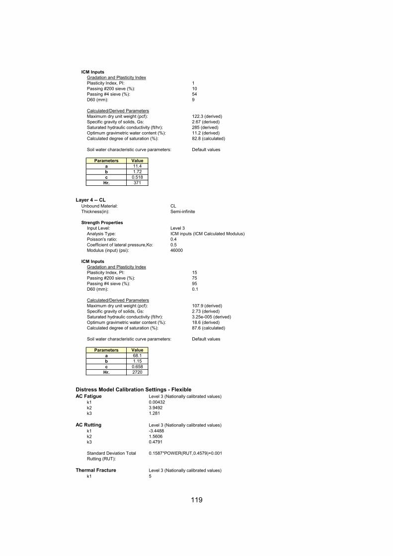
119
Value11.41.720.518371
Value68.11.150.6582720
0.004323.94921.281
-3.44881.56060.4791
5Thermal Fracture Level 3 (Nationally calibrated values)
k1
k2k3
Standard Deviation Total Rutting (RUT):
0.1587*POWER(RUT,0.4579)+0.001
k3
AC Rutting Level 3 (Nationally calibrated values)k1
AC Fatigue Level 3 (Nationally calibrated values)k1k2
bc
Hr.
Distress Model Calibration Settings - Flexible
Soil water characteristic curve parameters: Default values
Parametersa
Optimum gravimetric water content (%): 18.6 (derived)Calculated degree of saturation (%): 87.6 (calculated)
Specific gravity of solids, Gs: 2.73 (derived)Saturated hydraulic conductivity (ft/hr): 3.25e-005 (derived)
D60 (mm): 0.1
Calculated/Derived ParametersMaximum dry unit weight (pcf): 107.9 (derived)
Passing #200 sieve (%): 75Passing #4 sieve (%): 95
ICM InputsGradation and Plasticity IndexPlasticity Index, PI: 15
Coefficient of lateral pressure,Ko: 0.5Modulus (input) (psi): 46000
Analysis Type: ICM inputs (ICM Calculated Modulus)Poisson's ratio: 0.4
Thickness(in): Semi-infinite
Strength PropertiesInput Level: Level 3
Hr.
Layer 4 -- CLUnbound Material: CL
Parametersabc
Calculated degree of saturation (%): 82.8 (calculated)
Soil water characteristic curve parameters: Default values
Saturated hydraulic conductivity (ft/hr): 285 (derived)Optimum gravimetric water content (%): 11.2 (derived)
Calculated/Derived ParametersMaximum dry unit weight (pcf): 122.3 (derived)Specific gravity of solids, Gs: 2.67 (derived)
Passing #4 sieve (%): 54D60 (mm): 9
Plasticity Index, PI: 1Passing #200 sieve (%): 10
ICM InputsGradation and Plasticity Index

120
11
1.673
1.35
73.501000
1106000
1101000
0.04630.001190.18340.003840.007360.001150.387
0.0099950.0005180.0023518.360.96940.292
0.007320.076470.0001450.008420.0002120.229
C4 (CSM)C5 (CSM)Std. Dev (CSM)
IRI Flexible Pavements with CSMC1 (CSM)C2 (CSM)C3 (CSM)
C3 (ATB)C4 (ATB)C5 (ATB)Std. Dev (ATB)
Std. Dev (GB)
IRI Flexible Pavements with ATBC1 (ATB)C2 (ATB)
C3 (GB)C4 (GB)C5 (GB)C6 (GB)
IRIIRI Flexible Pavements with GB
C1 (GB)C2 (GB)
C3 (CSM)C4 (CSM)
Standard Deviation (CSM) CTB*1
32.7 + 995.1 /(1+exp(2-2*log(BOTTOM+0.0001)))
CSM CrackingC1 (CSM)C2 (CSM)
C2 (bottom)C3 (bottom)C4 (bottom)
Standard Deviation (TOP)
Standard Deviation (TOP) 200 + 2300/(1+exp(1.072-2.1654*log(TOP+0.0001)))
AC Bottom Up CrackingC1 (bottom)
C1 (top)C2 (top)C3 (top)C4 (top)
Fine-grain:k1
AC CrackingAC Top Down Cracking
Subgrade Rutting Level 3 (Nationally calibrated values)Granular:
k1
CSM Fatigue Level 3 (Nationally calibrated values)k1k2

121
Distress Target
Reliablity Target
Distress Predicted
Reliability Predicted Acceptable
172 90 127.1 96.28 Pass
1000 90 66.6 74.4 Fail
25 90 0 99.999 Pass
1000 90 1005 49.23 Fail25 90 N/A
0.25 90 0.4 7.19 Fail0.75 90 0.48 99.12 Pass
Permanent Deformation (AC Only) (in):Permanent Deformation (Total Pavement) (in):
AC Surface Down Cracking (Long. Cracking) (ft/500):AC Bottom Up Cracking (Alligator Cracking) (%):AC Thermal Fracture (Transverse Cracking) (ft/mi):Chemically Stabilized Layer (Fatigue Fracture)
Project: SITE18-New Design.dgpReliability Summary
Performance Criteria
Terminal IRI (in/mi)
Asphalt Sub-Layers Modulus Vs Time
0
500,000
1,000,000
1,500,000
2,000,000
2,500,000
3,000,000
3,500,000
4,000,000
4,500,000
5,000,000
0 18 36 54 72 90 108 126 144 162 180
Pavement Age (month)
Mod
ulus
(psi
)
AC1(1) h=0.5 AC1(2) h=0.5 AC1(3) h=1.0 AC1(4) h=1.0 AC1(5) h=1.0 AC1(6) h=4.0 AC1(7) h=5.0
Surface Down Cracking - Longitudinal
0
300
600
900
1200
1500
1800
2100
2400
2700
3000
0 18 36 54 72 90 108 126 144 162 180 198
Pavement Age (month)
Long
itudi
nal C
rack
ing
(ft/m
i)
Surface Depth = 0.5" Surface at Reliability Design Limit

122
Bottom Up Cracking - Alligator
0
10
20
30
40
50
60
70
80
90
100
0 18 36 54 72 90 108 126 144 162 180 198
Pavement Age (month)
Alli
gato
r Cra
ckin
g (%
)
Maximum Cracking Bottom Up Reliability Maximum Cracking Limit
Thermal Cracking: Total Length Vs Time
0
200
400
600
800
1000
1200
1400
1600
1800
2000
0 18 36 54 72 90 108 126 144 162 180 198
Pavement Age (month)
Tota
l Len
gth
(ft/m
i)
Thermal Crack Length Crack Length at Reliability Design Limit

123
Permanant Deformation: Rutting
0.00
0.10
0.20
0.30
0.40
0.50
0.60
0.70
0.80
0 18 36 54 72 90 108 126 144 162 180 198
Pavement Age (month)
Rut
ting
Dep
th (i
n)
SubTotalAC SubTotalBase SubTotalSG Total Rutting TotalRutReliability Total Rutting Design Limit
AC Rutting Design Value = 0.25Total Rutting Design Limit = 0.75
IRI
0
20
40
60
80
100
120
140
160
180
200
0 18 36 54 72 90 108 126 144 162 180 198
Pavement Age (month)
IRI (
in/m
i)
IRI IRI at Reliability Design Limit

124
Limit Reliability63
172 901000 90
25 901000 90
25 900.25 900.75 90
105613
507060
Class 4 Class 5 Class 6 Class 7 Class 8 Class 9 Class 10 Class 11 Class 12 Class 131.00 1.00 1.00 1.00 1.00 1.00 1.00 1.00 1.00 1.00 1.00 1.00 1.00 1.00 1.00 1.00 1.00 1.00 1.00 1.00 1.00 1.00 1.00 1.00 1.00 1.00 1.00 1.00 1.00 1.00 1.00 1.00 1.00 1.00 1.00 1.00 1.00 1.00 1.00 1.00 1.00 1.00 1.00 1.00 1.00 1.00 1.00 1.00 1.00 1.00 1.00 1.00 1.00 1.00 1.00 1.00 1.00 1.00 1.00 1.00 1.00 1.00 1.00 1.00 1.00 1.00 1.00 1.00 1.00 1.00 1.00 1.00 1.00 1.00 1.00 1.00 1.00 1.00 1.00 1.00 1.00 1.00 1.00 1.00 1.00 1.00 1.00 1.00 1.00 1.00 1.00 1.00 1.00 1.00 1.00 1.00 1.00 1.00 1.00 1.00 1.00 1.00 1.00 1.00 1.00 1.00 1.00 1.00 1.00 1.00 1.00 1.00 1.00 1.00 1.00 1.00 1.00 1.00 1.00 1.00
Midnight 2.3% Noon 5.9%1.3% 1:00 am 2.3% 1:00 pm 5.9%8.5% 2:00 am 2.3% 2:00 pm 5.9%2.8% 3:00 am 2.3% 3:00 pm 5.9%0.3% 4:00 am 2.3% 4:00 pm 4.6%7.6% 5:00 am 2.3% 5:00 pm 4.6%
74.0% 6:00 am 5.0% 6:00 pm 4.6%1.2% 7:00 am 5.0% 7:00 pm 4.6%3.4% 8:00 am 5.0% 8:00 pm 3.1%0.6% 9:00 am 5.0% 9:00 pm 3.1%
Project: SITE18-Rehabilitation.dgp
General Information Description:o Route: 81 South o County: Washington (number 95) o Length: 2640 ft o Number of lanes in each direction: 3 o Pavement Category: Flexible, 0-5 years o Traffic: TT 5,940 & AADT 20,000 (one way traffic) o AC overlay: 2in HMA:13in; Asphalt OGDL: 3in Agg. Base: 21in o Subgrade: orange-brown to yellow-brown sandy silty clay
Design Life 20 yearsExisting pavement construction: September, 1999Pavement overlay construction: September, 2001Traffic open: September, 2001Type of design Flexible
Analysis ParametersAnalysis type Probabilistic
Performance CriteriaInitial IRI (in/mi)Terminal IRI (in/mi)AC Surface Down Cracking (Long. Cracking) (ft/500):AC Bottom Up Cracking (Alligator Cracking) (%):AC Thermal Fracture (Transverse Cracking) (ft/mi):Chemically Stabilized Layer (Fatigue Fracture)Permanent Deformation (AC Only) (in):Permanent Deformation (Total Pavement) (in):
Location: Washington, VAProject ID: SITE18Section ID:
Principal Arterials - Interstate and Defense RoutesDate: 2/28/2005
Station/milepost format: Miles: 0.000 1.5Station/milepost end: 1Traffic direction: South bound
Default Input LevelDefault input level Level 3, Default and historical agency values.
Traffic Initial two-way aadtt:Number of lanes in design direction:Percent of trucks in design direction (%):Percent of trucks in design lane (%):Operational speed (mph):
Traffic -- Volume Adjustment FactorsMonthly Adjustment Factors (Level 3, Default MAF)
Vehicle ClassMonth
JanuaryFebruaryMarchAprilMayJuneJulyAugustSeptemberOctoberNovemberDecember
Vehicle Class Distribution Hourly truck traffic distribution(Level 3, Default Distribution) by period beginning:
AADTT distribution by vehicle classClass 4Class 5Class 6Class 7Class 8Class 9Class 10Class 11Class 12

125
4.0%4.0%4.0%4.0%4.0%4.0%4.0%4.0%4.0%4.0%
18
1012
1.62 0.39 0.00 0.00 2.00 0.00 0.00 0.00 1.02 0.99 0.00 0.00 1.00 0.26 0.83 0.00 2.38 0.67 0.00 0.00 1.13 1.93 0.00 0.00 1.19 1.09 0.89 0.00 4.29 0.26 0.06 0.00 3.52 1.14 0.06 0.00 2.15 2.13 0.35 0.00
8.5
12
120120
51.649.249.2
36.7-81.99205015
Traffic Growth Factor
Vehicle Class
Growth Rate
GrowthFunction
Class 4 CompoundClass 5 CompoundClass 6 CompoundClass 7 CompoundClass 8 CompoundClass 9 CompoundClass 10 CompoundClass 11 CompoundClass 12 CompoundClass 13 Compound
Traffic -- Axle Load Distribution FactorsLevel 3: Default
Traffic -- General Traffic InputsMean wheel location (inches from the lane marking):Traffic wander standard deviation (in):Design lane width (ft):
Number of Axles per Truck
Quad Axle
Class 4Class 5Class 6
Vehicle Class
Single Axle
Tandem Axle
Tridem Axle
Class 7Class 8Class 9Class 10Class 11Class 12Class 13
Axle ConfigurationAverage axle width (edge-to-edge) outside dimensions,ft):Dual tire spacing (in):
Axle ConfigurationSingle Tire (psi):Dual Tire (psi):
Average Axle SpacingTandem axle(psi):Tridem axle(psi):Quad axle(psi):
Climate icm file:
site18-02Latitude (degrees.minutes)Longitude (degrees.minutes)Elevation (ft)Depth of water table (ft)
Structure--Design Features
Structure--Layers Layer 1 -- Asphalt concrete
Material type: Asphalt concreteLayer thickness (in): 2

126
General PropertiesGeneralReference temperature (F°): 70
Volumetric Properties as BuiltEffective binder content (%): 11Air voids (%): 4.3Total unit weight (pcf): 148
Poisson's ratio: 0.35 (user entered)
Thermal PropertiesThermal conductivity asphalt (BTU/hr-ft-F°): 0.67Heat capacity asphalt (BTU/lb-F°): 0.23
Asphalt MixCumulative % Retained 3/4 inch sieve: 0Cumulative % Retained 3/8 inch sieve: 12Cumulative % Retained #4 sieve: 45% Passing #200 sieve: 6
Asphalt BinderOption: Conventional viscosity gradeViscosity Grade AC 20A 10.7709 (correlated)VTS: -3.6017 (correlated)
Layer 2 -- Asphalt concrete (existing)Material type: Asphalt concrete (existing)Layer thickness (in): 14.5
General PropertiesGeneralReference temperature (F°): 70
Volumetric Properties as BuiltEffective binder content (%): 10Air voids (%): 6Total unit weight (pcf): 163
Poisson's ratio: 0.35 (user entered)
Thermal PropertiesThermal conductivity asphalt (BTU/hr-ft-F°): 0.67Heat capacity asphalt (BTU/lb-F°): 0.23
Asphalt MixCumulative % Retained 3/4 inch sieve: 21Cumulative % Retained 3/8 inch sieve: 40Cumulative % Retained #4 sieve: 57% Passing #200 sieve: 4
Asphalt BinderOption: Conventional viscosity gradeViscosity Grade AC 20A 10.7709 (correlated)VTS: -3.6017 (correlated)
Layer 3 -- Crushed stoneUnbound Material: Crushed stoneThickness(in): 21
Strength PropertiesInput Level: Level 3Analysis Type: ICM inputs (ICM Calculated Modulus)Poisson's ratio: 0.35Coefficient of lateral pressure,Ko: 0.5Modulus (input) (psi): 90000

127
Value11.41.72
0.518371
Value68.11.15
0.6582720
0.004323.94921.281
ICM InputsGradation and Plasticity IndexPlasticity Index, PI: 1Passing #200 sieve (%): 10Passing #4 sieve (%): 54D60 (mm): 9
Calculated/Derived ParametersMaximum dry unit weight (pcf): 122.3 (derived)Specific gravity of solids, Gs: 2.67 (derived)Saturated hydraulic conductivity (ft/hr): 285 (derived)Optimum gravimetric water content (%): 11.2 (derived)Calculated degree of saturation (%): 82.8 (calculated)
Soil water characteristic curve parameters: Default values
Parametersabc
Hr.
Layer 4 -- CLUnbound Material: CLThickness(in): Semi-infinite
Strength PropertiesInput Level: Level 3Analysis Type: ICM inputs (ICM Calculated Modulus)Poisson's ratio: 0.4Coefficient of lateral pressure,Ko: 0.5Modulus (input) (psi): 46000
ICM InputsGradation and Plasticity IndexPlasticity Index, PI: 15Passing #200 sieve (%): 75Passing #4 sieve (%): 95D60 (mm): 0.1
Calculated/Derived ParametersMaximum dry unit weight (pcf): 107.9 (derived)Specific gravity of solids, Gs: 2.73 (derived)Saturated hydraulic conductivity (ft/hr): 3.25e-005 (derived)Optimum gravimetric water content (%): 18.6 (derived)Calculated degree of saturation (%): 87.6 (calculated)
Soil water characteristic curve parameters: Default values
Parametersabc
Hr.
Distress Model Calibration Settings - Flexible AC Fatigue Level 3 (Nationally calibrated values)
k1k2k3

128
-3.44881.56060.4791
5
11
1.673
1.35
73.501000
1106000
1101000
0.0115050.0035993.4300570.0007230.0112419.042440.179
0.0082630.0221831.330410.197
AC Rutting Level 3 (Nationally calibrated values)k1k2k3
Standard Deviation Total Rutting (RUT):
0.1587*POWER(RUT,0.4579)+0.001
Thermal Fracture Level 3 (Nationally calibrated values)k1
Std. Dev. (THERMAL): 0.2474 * THERMAL + 10.619
CSM Fatigue Level 3 (Nationally calibrated values)k1k2
Subgrade Rutting Level 3 (Nationally calibrated values)Granular:
k1Fine-grain:
k1
AC CrackingAC Top Down Cracking
C1 (top)C2 (top)C3 (top)C4 (top)
Standard Deviation (TOP) 200 + 2300/(1+exp(1.072-2.1654*log(TOP+0.0001)))
AC Bottom Up CrackingC1 (bottom)C2 (bottom)C3 (bottom)C4 (bottom)
Standard Deviation (TOP) 32.7 + 995.1 /(1+exp(2-2*log(BOTTOM+0.001)))
CSM CrackingC1 (CSM)C2 (CSM)C3 (CSM)C4 (CSM)
Standard Deviation (CSM) CTB*11
IRIIRI Rehabilitation over Flexible
C1 (Flexible)C2 (Flexible)C3 (Flexible)C4 (Flexible)C5 (Flexible)C6 (Flexible)Std. Dev (Flexible)
IRI Rehabilitation over RigidC1 (Rigid)C2 (Rigid)C3 (Rigid)Std. Dev (Rigid)
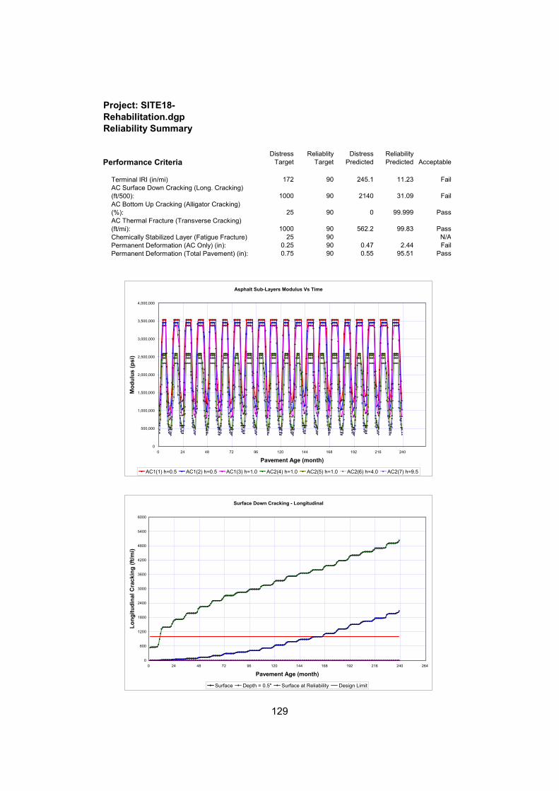
129
Distress Target
Reliablity Target
Distress Predicted
Reliability Predicted Acceptable
172 90 245.1 11.23 Fail
1000 90 2140 31.09 Fail
25 90 0 99.999 Pass
1000 90 562.2 99.83 Pass25 90 N/A
0.25 90 0.47 2.44 Fail0.75 90 0.55 95.51 Pass
Project: SITE18-Rehabilitation.dgpReliability Summary
Performance Criteria
Terminal IRI (in/mi)
Permanent Deformation (AC Only) (in):Permanent Deformation (Total Pavement) (in):
AC Surface Down Cracking (Long. Cracking) (ft/500):AC Bottom Up Cracking (Alligator Cracking) (%):AC Thermal Fracture (Transverse Cracking) (ft/mi):Chemically Stabilized Layer (Fatigue Fracture)
Asphalt Sub-Layers Modulus Vs Time
0
500,000
1,000,000
1,500,000
2,000,000
2,500,000
3,000,000
3,500,000
4,000,000
0 24 48 72 96 120 144 168 192 216 240
Pavement Age (month)
Mod
ulus
(psi
)
AC1(1) h=0.5 AC1(2) h=0.5 AC1(3) h=1.0 AC2(4) h=1.0 AC2(5) h=1.0 AC2(6) h=4.0 AC2(7) h=9.5
Surface Down Cracking - Longitudinal
0
600
1200
1800
2400
3000
3600
4200
4800
5400
6000
0 24 48 72 96 120 144 168 192 216 240 264
Pavement Age (month)
Long
itudi
nal C
rack
ing
(ft/m
i)
Surface Depth = 0.5" Surface at Reliability Design Limit

130
Bottom Up Cracking - Alligator
0
10
20
30
40
50
60
70
80
90
100
0 24 48 72 96 120 144 168 192 216 240 264
Pavement Age (month)
Alli
gato
r Cra
ckin
g (%
)
Maximum Cracking Bottom Up Reliability Maximum Cracking Limit
Thermal Cracking: Total Length Vs Time
0
200
400
600
800
1000
1200
1400
1600
1800
2000
0 24 48 72 96 120 144 168 192 216 240 264
Pavement Age (month)
Tota
l Len
gth
(ft/m
i)
Thermal Crack Length Crack Length at Reliability Design Limit

131
Permanant Deformation: Rutting
0.00
0.10
0.20
0.30
0.40
0.50
0.60
0.70
0.80
0 24 48 72 96 120 144 168 192 216 240 264
Pavement Age (month)
Rut
ting
Dep
th (i
n)
SubTotalAC SubTotalBase SubTotalSG Total Rutting TotalRutReliability Total Rutting Design Limit
AC Rutting Design Value = 0.25Total Rutting Design Limit = 0.75
IRI
0
30
60
90
120
150
180
210
240
270
300
0 24 48 72 96 120 144 168 192 216 240 264
Pavement Age (month)
IRI (
in/m
i)
IRI IRI at Reliability Design Limit

132
Limit Reliability63
172 9010 90
8862
508060
Class 4 Class 5 Class 6 Class 7 Class 8 Class 9 Class 10 Class 11 Class 12 Class 131.00 1.00 1.00 1.00 1.00 1.00 1.00 1.00 1.00 1.00 1.00 1.00 1.00 1.00 1.00 1.00 1.00 1.00 1.00 1.00 1.00 1.00 1.00 1.00 1.00 1.00 1.00 1.00 1.00 1.00 1.00 1.00 1.00 1.00 1.00 1.00 1.00 1.00 1.00 1.00 1.00 1.00 1.00 1.00 1.00 1.00 1.00 1.00 1.00 1.00 1.00 1.00 1.00 1.00 1.00 1.00 1.00 1.00 1.00 1.00 1.00 1.00 1.00 1.00 1.00 1.00 1.00 1.00 1.00 1.00 1.00 1.00 1.00 1.00 1.00 1.00 1.00 1.00 1.00 1.00 1.00 1.00 1.00 1.00 1.00 1.00 1.00 1.00 1.00 1.00 1.00 1.00 1.00 1.00 1.00 1.00 1.00 1.00 1.00 1.00 1.00 1.00 1.00 1.00 1.00 1.00 1.00 1.00 1.00 1.00 1.00 1.00 1.00 1.00 1.00 1.00 1.00 1.00 1.00 1.00
Midnight 2.3% Noon 5.9%1.3% 1:00 am 2.3% 1:00 pm 5.9%8.5% 2:00 am 2.3% 2:00 pm 5.9%2.8% 3:00 am 2.3% 3:00 pm 5.9%0.3% 4:00 am 2.3% 4:00 pm 4.6%7.6% 5:00 am 2.3% 5:00 pm 4.6%
74.0% 6:00 am 5.0% 6:00 pm 4.6%1.2% 7:00 am 5.0% 7:00 pm 4.6%3.4% 8:00 am 5.0% 8:00 pm 3.1%0.6% 9:00 am 5.0% 9:00 pm 3.1%0.3% 10:00 am 5.9% 10:00 pm 3.1%
11:00 am 5.9% 11:00 pm 3.1%Class 13
Traffic Growth Factor
Class 9Class 10Class 11Class 12
Class 5Class 6Class 7Class 8
(Level 3, Default Distribution) by period beginning:AADTT distribution by vehicle classClass 4
NovemberDecember
Vehicle Class Distribution Hourly truck traffic distribution
JulyAugustSeptemberOctober
MarchAprilMayJune
Vehicle ClassMonth
JanuaryFebruary
Percent of trucks in design lane (%):Operational speed (mph):
Traffic -- Volume Adjustment FactorsMonthly Adjustment Factors (Level 3, Default MAF)
Traffic Initial two-way aadtt:Number of lanes in design direction:Percent of trucks in design direction (%):
Traffic direction: East bound
Default Input LevelDefault input level Level 3, Default and historical agency values.
Station/milepost begin: 12.99Station/milepost end: 13.37
Station/milepost format: Miles: 0.000
Principal Arterials - Interstate and Defense RoutesDate: 2/28/2005
Project ID: SITE02Section ID:
Terminal IRI (in/mi)CRCP Punchouts (per mi)
Location: Albermarle, Charlottesville, VA
Analysis type Probabilistic
Performance CriteriaInitial IRI (in/mi)
Type of design CRCP
Analysis Parameters
Project: SITE02-New Design.dgp
General Information Description:(SITE02-01 Original Design) o Route: I64 East o County: Albemarle, Charlottesville (number 2) o Length: 2640 ft o Number of lanes in each direction: 2 o Pavement Category: Composite CRCP older than 20 years, w/surface older than 10 years o Traffic: TT 1,680, AADT 15,000 o AC Overlay: 4.5in CRCP:8.25in o Subgrade: reddish-brown sandy salt w/mica
Design Life 20 yearsPavement construction: September, 1970Traffic open: October, 1970

133
18
1012
1.62 0.39 0.00 0.00 2.00 0.00 0.00 0.00 1.02 0.99 0.00 0.00 1.00 0.26 0.83 0.00 2.38 0.67 0.00 0.00 1.13 1.93 0.00 0.00 1.19 1.09 0.89 0.00 4.29 0.26 0.06 0.00 3.52 1.14 0.06 0.00 2.15 2.13 0.35 0.00
8.5
12
120120
51.649.249.2
Short Medium Long12 15 18
33% 33% 34%
38.06-78.564025
-10Asphalt
0.70.6254
0.85Structure--ICM Properties
Surface shortwave absorptivity:
Drainage Parameters
Base/slab friction coefficient: 4
Crack SpacingCracking Model Generate using model.
Base type: GranularErodibility index: Fairly Erodable (4)
Percent steel (%):Bar diameter (in):Steel depth (in):
Base Properties
Structure--Design Features Permanent curl/warp effective temperature difference (°F):Shoulder type:
Steel Reinforcement
Latitude (degrees.minutes)Longitude (degrees.minutes)Elevation (ft)Depth of water table (ft)
Climate icm file:
Site02-01
Quad axle(psi):
Wheelbase Truck Tractor
Average Axle Spacing (ft)Percent of trucks
Dual Tire (psi):
Average Axle SpacingTandem axle(psi):Tridem axle(psi):
Average axle width (edge-to-edge) outside dimensions,ft):Dual tire spacing (in):
Axle ConfigurationSingle Tire (psi):
Class 11Class 12Class 13
Axle Configuration
Class 7Class 8Class 9Class 10
Quad Axle
Class 4Class 5Class 6
Vehicle Class
Single Axle
Tandem Axle
Tridem Axle
Mean wheel location (inches from the lane marking):Traffic wander standard deviation (in):Design lane width (ft):
Number of Axles per Truck
Traffic -- Axle Load Distribution FactorsLevel 3: Default
Traffic -- General Traffic Inputs

134
Value46.91.21
0.6351760Hr.
Parametersabc
Calculated degree of saturation (%): 87.2 (calculated)
Soil water characteristic curve parameters: Default values
Saturated hydraulic conductivity (ft/hr): 3.25e-005 (derived)Optimum gravimetric water content (%): 16.9 (derived)
Calculated/Derived ParametersMaximum dry unit weight (pcf): 111.2 (derived)Specific gravity of solids, Gs: 2.72 (derived)
Passing #4 sieve (%): 95D60 (mm): 0.05
Plasticity Index, PI: 10Passing #200 sieve (%): 80
Modulus (input) (psi): 38000
ICM InputsGradation and Plasticity Index
Poisson's ratio: 0.35Coefficient of lateral pressure,Ko: 0.5
Strength PropertiesInput Level: Level 3Analysis Type: ICM inputs (ICM Calculated Modulus)
Layer 2 -- MLUnbound Material: MLThickness(in): 12
28-day PCC modulus of rupture (psi): n/a28-day PCC compressive strength (psi): 4120
Curing method: Curing compound
Strength PropertiesInput level: Level 3
Reversible shrinkage (% of ultimate shrinkage): 50Time to develop 50% of ultimate shrinkage (days): 35
PCC zero-stress temperature (F°) DerivedUltimate shrinkage at 40% R.H (microstrain) Derived
Water/cement ratio: 0.45Aggregate type: Limestone
Mix PropertiesCement type: Type IICementitious material content (lb/yd^3): 564
Thermal conductivity (BTU/hr-ft-F°) : 1.25Heat capacity (BTU/lb-F°): 0.28
Poisson's ratio 0.2
Thermal PropertiesCoefficient of thermal expansion (per F° x 10- 6): 5.5
Layer thickness (in): 8.25Unit weight (pcf): 150
Structure--Layers Layer 1 -- CRCP
General PropertiesPCC material CRCP

135
21.22
105.26324
-0.38158
1
13.15
28.3510.03
5.4
C3C4Standard deviation in initial IRI (in/mile):
4.04*POWER(PO, 0.3825)
IRI(crcp)C1C2
Crack WidthC6
Reliability (PO)Std. Dev.
PunchoutC3C4C5
PunchoutsFatigue
C1C2
Distress Model Calibration Settings - Rigid (new)
Predicted Punchout
0.0
4.1
8.2
12.3
16.4
20.5
24.6
28.7
32.8
36.9
41.0
0 2 4 6 8 10 12 14 16 18 20 22
Pavement age, years
Punc
hout
per
mile
Punchout Punchout at specified reliability Punchout Limit
Distress Target
Reliablity Target
Distress Predicted
Reliability Predicted Acceptable
172 90 112 94 Pass10 90 23.5 15.82 FailCRCP Punchouts (per mi)
Project: SITE02-New Design.dgpReliability Summary
Performance Criteria
Terminal IRI (in/mi)

136
IRI
0
18
36
54
72
90
108
126
144
162
180
0 2 4 6 8 10 12 14 16 18 20 22 24
Pavement age, years
IRI,
in/m
ile
IRI IRI at specified reliability IRI Limit

137
Limit Reliability63
172 901000 90
25 901000 90
25 900.25 900.75 90
20992
508060
Class 4 Class 5 Class 6 Class 7 Class 8 Class 9 Class 10 Class 11 Class 12 Class 131.00 1.00 1.00 1.00 1.00 1.00 1.00 1.00 1.00 1.00 1.00 1.00 1.00 1.00 1.00 1.00 1.00 1.00 1.00 1.00 1.00 1.00 1.00 1.00 1.00 1.00 1.00 1.00 1.00 1.00 1.00 1.00 1.00 1.00 1.00 1.00 1.00 1.00 1.00 1.00 1.00 1.00 1.00 1.00 1.00 1.00 1.00 1.00 1.00 1.00 1.00 1.00 1.00 1.00 1.00 1.00 1.00 1.00 1.00 1.00 1.00 1.00 1.00 1.00 1.00 1.00 1.00 1.00 1.00 1.00 1.00 1.00 1.00 1.00 1.00 1.00 1.00 1.00 1.00 1.00 1.00 1.00 1.00 1.00 1.00 1.00 1.00 1.00 1.00 1.00 1.00 1.00 1.00 1.00 1.00 1.00 1.00 1.00 1.00 1.00 1.00 1.00 1.00 1.00 1.00 1.00 1.00 1.00 1.00 1.00 1.00 1.00 1.00 1.00 1.00 1.00 1.00 1.00 1.00 1.00
Midnight 2.3% Noon 5.9%1.3% 1:00 am 2.3% 1:00 pm 5.9%8.5% 2:00 am 2.3% 2:00 pm 5.9%2.8% 3:00 am 2.3% 3:00 pm 5.9%0.3% 4:00 am 2.3% 4:00 pm 4.6%7.6% 5:00 am 2.3% 5:00 pm 4.6%
74.0% 6:00 am 5.0% 6:00 pm 4.6%1.2% 7:00 am 5.0% 7:00 pm 4.6%3.4% 8:00 am 5.0% 8:00 pm 3.1%0.6% 9:00 am 5.0% 9:00 pm 3.1%
Project: SITE02-Rehabilitation.dgp
General Information Description:(SITE02-01 Overlay Design) o Route: I64 East o County: Albemarle, Charlottesville (number 2) o Length: 2640 ft o Number of lanes in each direction: 2 o Pavement Category: Composite CRCP older than 20 years, w/surface older than 10 years o Traffic: TT 1,680, AADT 15,000 o AC Overlay: 4.5in CRCP:8.25in o Subgrade: reddish-brown sandy salt w/mica
Design Life 20 yearsExisting pavement construction: September, 1970Pavement overlay construction: September, 1992Traffic open: October, 1992Type of design Flexible
Analysis ParametersAnalysis type Probabilistic
Performance CriteriaInitial IRI (in/mi)Terminal IRI (in/mi)AC Surface Down Cracking (Long. Cracking) (ft/500):AC Bottom Up Cracking (Alligator Cracking) (%):AC Thermal Fracture (Transverse Cracking) (ft/mi):Chemically Stabilized Layer (Fatigue Fracture)Permanent Deformation (AC Only) (in):Permanent Deformation (Total Pavement) (in):
Location: Albermarle, Charlottesville, VAProject ID: SITE02Section ID:
Principal Arterials - Interstate and Defense RoutesDate: 2/28/2005
Station/milepost format: Miles: 0.000Station/milepost begin: 12.99Station/milepost end: 13.37Traffic direction: East bound
Default Input LevelDefault input level Level 3, Default and historical agency values.
Traffic Initial two-way aadtt:Number of lanes in design direction:Percent of trucks in design direction (%):Percent of trucks in design lane (%):Operational speed (mph):
Traffic -- Volume Adjustment FactorsMonthly Adjustment Factors (Level 3, Default MAF)
Vehicle ClassMonth
JanuaryFebruaryMarchAprilMayJuneJulyAugustSeptemberOctoberNovemberDecember
Vehicle Class Distribution Hourly truck traffic distribution(Level 3, Default Distribution) by period beginning:
AADTT distribution by vehicle classClass 4Class 5Class 6Class 7Class 8Class 9Class 10Class 11Class 12
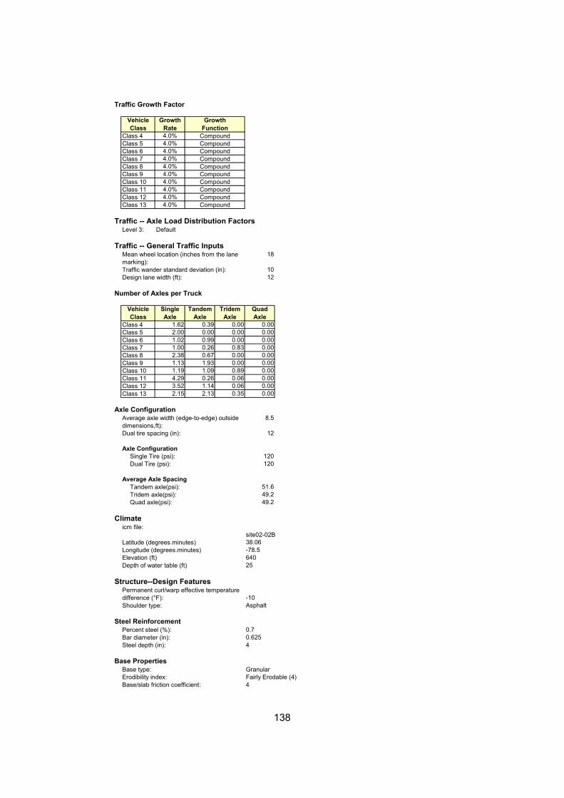
138
4.0%4.0%4.0%4.0%4.0%4.0%4.0%4.0%4.0%4.0%
18
1012
1.62 0.39 0.00 0.00 2.00 0.00 0.00 0.00 1.02 0.99 0.00 0.00 1.00 0.26 0.83 0.00 2.38 0.67 0.00 0.00 1.13 1.93 0.00 0.00 1.19 1.09 0.89 0.00 4.29 0.26 0.06 0.00 3.52 1.14 0.06 0.00 2.15 2.13 0.35 0.00
8.5
12
120120
51.649.249.2
38.06-78.564025
-10Asphalt
0.70.6254
Traffic Growth Factor
Vehicle Class
Growth Rate
GrowthFunction
Class 4 CompoundClass 5 CompoundClass 6 CompoundClass 7 CompoundClass 8 CompoundClass 9 CompoundClass 10 CompoundClass 11 CompoundClass 12 CompoundClass 13 Compound
Traffic -- Axle Load Distribution FactorsLevel 3: Default
Traffic -- General Traffic InputsMean wheel location (inches from the lane marking):Traffic wander standard deviation (in):Design lane width (ft):
Number of Axles per Truck
Quad Axle
Class 4Class 5Class 6
Vehicle Class
Single Axle
Tandem Axle
Tridem Axle
Class 7Class 8Class 9Class 10Class 11Class 12Class 13
Axle ConfigurationAverage axle width (edge-to-edge) outside dimensions,ft):Dual tire spacing (in):
Axle ConfigurationSingle Tire (psi):Dual Tire (psi):
Average Axle SpacingTandem axle(psi):Tridem axle(psi):Quad axle(psi):
Climate icm file:
site02-02BLatitude (degrees.minutes)Longitude (degrees.minutes)Elevation (ft)Depth of water table (ft)
Structure--Design Features Permanent curl/warp effective temperature difference (°F):Shoulder type:
Steel ReinforcementPercent steel (%):Bar diameter (in):Steel depth (in):
Base PropertiesBase type: GranularErodibility index: Fairly Erodable (4)Base/slab friction coefficient: 4

139
0.85
Crack SpacingCracking Model Generate using model.
Structure--ICM PropertiesSurface shortwave absorptivity:
Drainage ParametersInfiltration: Minor (10%)Drainage path length (ft): 12Pavement cross slope (%): 2
Structure--Layers Layer 1 -- Asphalt concrete
Material type: Asphalt concreteLayer thickness (in): 4.5
General PropertiesGeneralReference temperature (F°): 70
Volumetric Properties as BuiltEffective binder content (%): 11Air voids (%): 4.3Total unit weight (pcf): 148
Poisson's ratio: 0.35 (user entered)
Thermal PropertiesThermal conductivity asphalt (BTU/hr-ft-F°): 0.67Heat capacity asphalt (BTU/lb-F°): 0.23
Asphalt MixCumulative % Retained 3/4 inch sieve: 0Cumulative % Retained 3/8 inch sieve: 12Cumulative % Retained #4 sieve: 45% Passing #200 sieve: 5
Asphalt BinderOption: Conventional viscosity gradeViscosity Grade AC 30A 10.6316 (correlated)VTS: -3.548 (correlated)
Layer 2 -- CRCP (existing)General Properties
PCC material CRCP (existing)Layer thickness (in): 8.25Unit weight (pcf): 150Poisson's ratio 0.2
Thermal PropertiesCoefficient of thermal expansion (per F° x 10- 6): 5.5Thermal conductivity (BTU/hr-ft-F°) : 1.25Heat capacity (BTU/lb-F°): 0.28
Mix PropertiesCement type: Type IICementitious material content (lb/yd^3): 564Water/cement ratio: 0.45Aggregate type: LimestonePCC zero-stress temperature (F°) DerivedUltimate shrinkage at 40% R.H (microstrain) DerivedReversible shrinkage (% of ultimate shrinkage): 50Time to develop 50% of ultimate shrinkage (days): 35Curing method: Curing compound
Strength PropertiesInput level: Level 328-day PCC modulus of rupture (psi): n/a28-day PCC compressive strength (psi): 4120
Layer 3 -- MLUnbound Material: MLThickness(in): 12
Strength PropertiesInput Level: Level 3Analysis Type: ICM inputs (ICM Calculated Modulus)Poisson's ratio: 0.35Coefficient of lateral pressure,Ko: 0.5Modulus (input) (psi): 38000

140
Value46.91.210.6351760
Value46.91.210.6351760
0.004323.94921.281
-3.44881.56060.4791
5
ICM InputsGradation and Plasticity IndexPlasticity Index, PI: 10Passing #200 sieve (%): 80Passing #4 sieve (%): 95D60 (mm): 0.05
Calculated/Derived ParametersMaximum dry unit weight (pcf): 111.2 (derived)Specific gravity of solids, Gs: 2.72 (derived)Saturated hydraulic conductivity (ft/hr): 3.25e-005 (derived)Optimum gravimetric water content (%): 16.9 (derived)Calculated degree of saturation (%): 87.2 (calculated)
Soil water characteristic curve parameters: Default values
Parametersabc
Hr.
Layer 4 -- MLUnbound Material: MLThickness(in): Semi-infinite
Strength PropertiesInput Level: Level 3Analysis Type: ICM inputs (ICM Calculated Modulus)Poisson's ratio: 0.35Coefficient of lateral pressure,Ko: 0.5Modulus (input) (psi): 38000
ICM InputsGradation and Plasticity IndexPlasticity Index, PI: 10Passing #200 sieve (%): 80Passing #4 sieve (%): 95D60 (mm): 0.05
Calculated/Derived ParametersMaximum dry unit weight (pcf): 111.2 (derived)Specific gravity of solids, Gs: 2.72 (derived)Saturated hydraulic conductivity (ft/hr): 3.25e-005 (derived)Optimum gravimetric water content (%): 16.9 (derived)Calculated degree of saturation (%): 87.2 (calculated)
Soil water characteristic curve parameters: Default values
Parametersabc
Hr.
Distress Model Calibration Settings - Flexible AC Fatigue Level 3 (Nationally calibrated values)
k1k2k3
AC Rutting Level 3 (Nationally calibrated values)k1k2k3
Standard Deviation Total Rutting (RUT):
0.1587*POWER(RUT,0.4579)+0.001
Thermal Fracture Level 3 (Nationally calibrated values)k1

141
1.673
1.35
73.501000
1106000
1101000
0.0115050.0035993.4300570.0007230.0112419.042440.179
0.0082630.0221831.330410.197
Subgrade Rutting Level 3 (Nationally calibrated values)Granular:
k1Fine-grain:
k1
AC CrackingAC Top Down Cracking
C1 (top)C2 (top)C3 (top)C4 (top)
Standard Deviation (TOP) 200 + 2300/(1+exp(1.072-2.1654*log(TOP+0.0001)))
AC Bottom Up CrackingC1 (bottom)C2 (bottom)C3 (bottom)C4 (bottom)
Standard Deviation (TOP) 32.7 + 995.1 /(1+exp(2-2*log(BOTTOM+0.001)))
CSM CrackingC1 (CSM)C2 (CSM)C3 (CSM)C4 (CSM)
Standard Deviation (CSM) CTB*11
IRIIRI Rehabilitation over Flexible
C1 (Flexible)C2 (Flexible)C3 (Flexible)C4 (Flexible)C5 (Flexible)C6 (Flexible)Std. Dev (Flexible)
IRI Rehabilitation over RigidC1 (Rigid)C2 (Rigid)C3 (Rigid)Std. Dev (Rigid)

142
Distress Target
Reliablity Target
Distress Predicted
Reliability Predicted Acceptable
172 90 94 99.999 Pass
1000 90 0 99.999 Pass
25 90 0 99.999 Pass
1000 90 1 99.999 Pass25 90 N/A
0.25 90 0.56 0.53 Fail0.75 90 0.56 93.36 Pass
Project: SITE02-Rehabilitation.dgpReliability Summary
Performance Criteria
Terminal IRI (in/mi)
Permanent Deformation (AC Only) (in):Permanent Deformation (Total Pavement) (in):
AC Surface Down Cracking (Long. Cracking) (ft/500):AC Bottom Up Cracking (Alligator Cracking) (%):AC Thermal Fracture (Transverse Cracking) (ft/mi):Chemically Stabilized Layer (Fatigue Fracture)
Asphalt Sub-Layers Modulus Vs Time
0
500,000
1,000,000
1,500,000
2,000,000
2,500,000
3,000,000
3,500,000
4,000,000
0 24 48 72 96 120 144 168 192 216 240
Pavement Age (month)
Mod
ulus
(psi
)
AC1(1) h=0.5 AC1(2) h=0.5 AC1(3) h=1.0 AC1(4) h=1.0 AC1(5) h=1.5
Surface Down Cracking - Longitudinal
0
200
400
600
800
1000
1200
1400
1600
1800
2000
0 24 48 72 96 120 144 168 192 216 240 264
Pavement Age (month)
Long
itudi
nal C
rack
ing
(ft/m
i)
Surface Depth = 0.5" Surface at Reliability Design Limit

143
Bottom Up Cracking - Alligator
0
10
20
30
40
50
60
70
80
90
100
0 24 48 72 96 120 144 168 192 216 240 264
Pavement Age (month)
Alli
gato
r Cra
ckin
g (%
)
Maximum Cracking Bottom Up Reliability Maximum Cracking Limit
Thermal Cracking: Total Length Vs Time
0
200
400
600
800
1000
1200
1400
1600
1800
2000
0 24 48 72 96 120 144 168 192 216 240 264
Pavement Age (month)
Tota
l Len
gth
(ft/m
i)
Thermal Crack Length Crack Length at Reliability Design Limit
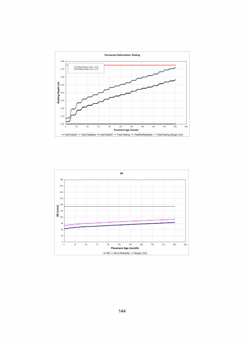
144
Permanant Deformation: Rutting
0.00
0.10
0.20
0.30
0.40
0.50
0.60
0.70
0.80
0 24 48 72 96 120 144 168 192 216 240 264
Pavement Age (month)
Rut
ting
Dep
th (i
n)
SubTotalAC SubTotalBase SubTotalSG Total Rutting TotalRutReliability Total Rutting Design Limit
AC Rutting Design Value = 0.25Total Rutting Design Limit = 0.75
IRI
0
30
60
90
120
150
180
210
240
270
300
0 24 48 72 96 120 144 168 192 216 240 264
Pavement Age (month)
IRI (
in/m
i)
IRI IRI at Reliability Design Limit

145
Limit Reliability63
172 9010 90
5022
508060
Class 4 Class 5 Class 6 Class 7 Class 8 Class 9 Class 10 Class 11 Class 12 Class 131.00 1.00 1.00 1.00 1.00 1.00 1.00 1.00 1.00 1.00 1.00 1.00 1.00 1.00 1.00 1.00 1.00 1.00 1.00 1.00 1.00 1.00 1.00 1.00 1.00 1.00 1.00 1.00 1.00 1.00 1.00 1.00 1.00 1.00 1.00 1.00 1.00 1.00 1.00 1.00 1.00 1.00 1.00 1.00 1.00 1.00 1.00 1.00 1.00 1.00 1.00 1.00 1.00 1.00 1.00 1.00 1.00 1.00 1.00 1.00 1.00 1.00 1.00 1.00 1.00 1.00 1.00 1.00 1.00 1.00 1.00 1.00 1.00 1.00 1.00 1.00 1.00 1.00 1.00 1.00 1.00 1.00 1.00 1.00 1.00 1.00 1.00 1.00 1.00 1.00 1.00 1.00 1.00 1.00 1.00 1.00 1.00 1.00 1.00 1.00 1.00 1.00 1.00 1.00 1.00 1.00 1.00 1.00 1.00 1.00 1.00 1.00 1.00 1.00 1.00 1.00 1.00 1.00 1.00 1.00
Midnight 2.3% Noon 5.9%1.3% 1:00 am 2.3% 1:00 pm 5.9%8.5% 2:00 am 2.3% 2:00 pm 5.9%2.8% 3:00 am 2.3% 3:00 pm 5.9%0.3% 4:00 am 2.3% 4:00 pm 4.6%7.6% 5:00 am 2.3% 5:00 pm 4.6%
74.0% 6:00 am 5.0% 6:00 pm 4.6%1.2% 7:00 am 5.0% 7:00 pm 4.6%3.4% 8:00 am 5.0% 8:00 pm 3.1%0.6% 9:00 am 5.0% 9:00 pm 3.1%0.3% 10:00 am 5.9% 10:00 pm 3.1%
11:00 am 5.9% 11:00 pm 3.1%Class 13
Class 9Class 10Class 11Class 12
Class 5Class 6Class 7Class 8
(Level 3, Default Distribution) by period beginning:AADTT distribution by vehicle classClass 4
NovemberDecember
Vehicle Class Distribution Hourly truck traffic distribution
JulyAugustSeptemberOctober
MarchAprilMayJune
Vehicle ClassMonth
JanuaryFebruary
Percent of trucks in design lane (%):Operational speed (mph):
Traffic -- Volume Adjustment FactorsMonthly Adjustment Factors (Level 3, Default MAF)
Traffic Initial two-way aadtt:Number of lanes in design direction:Percent of trucks in design direction (%):
Traffic direction: East bound
Default Input LevelDefault input level Level 3, Default and historical agency values.
Station/milepost begin: 14.69Station/milepost end: 15.19
Station/milepost format: Miles: 0.000
Principal Arterials - Interstate and Defense RoutesDate: 3/1/2005
Project ID: SITE05Section ID:
Terminal IRI (in/mi)CRCP Punchouts (per mi)
Location: New Kent, VA
Analysis type Probabilistic
Performance CriteriaInitial IRI (in/mi)
Type of design CRCP
Analysis Parameters
Project: SITE05-New Design.dgp
General Information Description:o Route: I64 East o County: New Kent (number 63) o Length: 2640 ft o Number of lanes in each direction: 2 o Pavement Category: Composite CRCP older than 20 years w/surface older than 10 years o Traffic: TT 880 & 800 AADT 21,000 o AC Overlay: 4.25in CRCP:8in Agg Base: 6in o Subgrade: dry silt to fine sand
Design Life 20 yearsPavement construction: August, 1972Traffic open: September, 1972

146
4.0%4.0%4.0%4.0%4.0%4.0%4.0%4.0%4.0%4.0%
18
1012
1.62 0.39 0.00 0.00 2.00 0.00 0.00 0.00 1.02 0.99 0.00 0.00 1.00 0.26 0.83 0.00 2.38 0.67 0.00 0.00 1.13 1.93 0.00 0.00 1.19 1.09 0.89 0.00 4.29 0.26 0.06 0.00 3.52 1.14 0.06 0.00 2.15 2.13 0.35 0.00
8.5
12
120120
51.649.249.2
Short Medium Long12 15 18
33% 33% 34%
37.54-77.0312340
-10Asphalt
0.7Percent steel (%):
Structure--Design Features Permanent curl/warp effective temperature difference (°F):Shoulder type:
Steel Reinforcement
Latitude (degrees.minutes)Longitude (degrees.minutes)Elevation (ft)Depth of water table (ft)
Climate icm file:
site05-01
Quad axle(psi):
Wheelbase Truck Tractor
Average Axle Spacing (ft)Percent of trucks
Dual Tire (psi):
Average Axle SpacingTandem axle(psi):Tridem axle(psi):
Average axle width (edge-to-edge) outside dimensions,ft):Dual tire spacing (in):
Axle ConfigurationSingle Tire (psi):
Class 11Class 12Class 13
Axle Configuration
Class 7Class 8Class 9Class 10
Quad Axle
Class 4Class 5Class 6
Vehicle Class
Single Axle
Tandem Axle
Tridem Axle
Mean wheel location (inches from the lane marking):Traffic wander standard deviation (in):Design lane width (ft):
Number of Axles per Truck
Traffic -- Axle Load Distribution FactorsLevel 3: Default
Traffic -- General Traffic Inputs
Class 12 CompoundClass 13 Compound
Class 10 CompoundClass 11 Compound
Class 8 CompoundClass 9 Compound
Class 6 CompoundClass 7 Compound
Class 4 CompoundClass 5 Compound
Traffic Growth Factor
Vehicle Class
Growth Rate
GrowthFunction

147
0.85
Value11.41.720.518371Hr.
Layer 3 -- MLUnbound Material: ML
Parametersabc
Calculated degree of saturation (%): 82.8 (calculated)
Soil water characteristic curve parameters: Default values
Saturated hydraulic conductivity (ft/hr): 294 (derived)Optimum gravimetric water content (%): 11.2 (derived)
Calculated/Derived ParametersMaximum dry unit weight (pcf): 122.3 (derived)Specific gravity of solids, Gs: 2.67 (derived)
Passing #4 sieve (%): 54D60 (mm): 9.5
Plasticity Index, PI: 1Passing #200 sieve (%): 10
Modulus (input) (psi): 68000
ICM InputsGradation and Plasticity Index
Poisson's ratio: 0.35Coefficient of lateral pressure,Ko: 0.5
Strength PropertiesInput Level: Level 3Analysis Type: ICM inputs (ICM Calculated Modulus)
Layer 2 -- Crushed stoneUnbound Material: Crushed stoneThickness(in): 6
28-day PCC modulus of rupture (psi): n/a28-day PCC compressive strength (psi): 4850
Curing method: Curing compound
Strength PropertiesInput level: Level 3
Reversible shrinkage (% of ultimate shrinkage): 50Time to develop 50% of ultimate shrinkage (days): 35
PCC zero-stress temperature (F°) DerivedUltimate shrinkage at 40% R.H (microstrain) Derived
Water/cement ratio: 0.45Aggregate type: Limestone
Mix PropertiesCement type: Type IICementitious material content (lb/yd^3): 564
Thermal conductivity (BTU/hr-ft-F°) : 1.25Heat capacity (BTU/lb-F°): 0.28
Poisson's ratio 0.2
Thermal PropertiesCoefficient of thermal expansion (per F° x 10- 6): 5.5
Layer thickness (in): 8Unit weight (pcf): 150
Structure--Layers Layer 1 -- CRCP
General PropertiesPCC material CRCP
Drainage path length (ft): 12Pavement cross slope (%): 2
Structure--ICM PropertiesSurface shortwave absorptivity:
Drainage ParametersInfiltration: Minor (10%)

148
Value46.91.210.6351760
21.22
105.26324
-0.38158
1
13.15
28.3510.03
5.4
C3C4Standard deviation in initial IRI (in/mile):
4.04*POWER(PO, 0.3825)
IRI(crcp)C1C2
Crack WidthC6
Reliability (PO)Std. Dev.
PunchoutC3C4C5
PunchoutsFatigue
C1C2
bc
Hr.
Distress Model Calibration Settings - Rigid (new)
Soil water characteristic curve parameters: Default values
Parametersa
Optimum gravimetric water content (%): 16.9 (derived)Calculated degree of saturation (%): 87.2 (calculated)
Specific gravity of solids, Gs: 2.72 (derived)Saturated hydraulic conductivity (ft/hr): 3.25e-005 (derived)
D60 (mm): 0.05
Calculated/Derived ParametersMaximum dry unit weight (pcf): 111.2 (derived)
Passing #200 sieve (%): 80Passing #4 sieve (%): 95
ICM InputsGradation and Plasticity IndexPlasticity Index, PI: 10
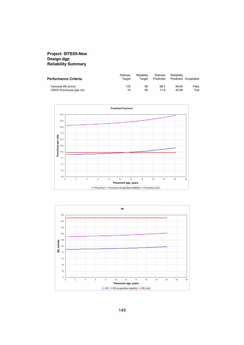
149
Predicted Punchout
0.0
2.6
5.1
7.7
10.2
12.8
15.3
17.9
20.4
23.0
25.5
0 2 4 6 8 10 12 14 16 18 20 22
Pavement age, years
Punc
hout
per
mile
Punchout Punchout at specified reliability Punchout Limit
Distress Target
Reliablity Target
Distress Predicted
Reliability Predicted Acceptable
172 90 88.3 99.64 Pass10 90 11.8 42.99 FailCRCP Punchouts (per mi)
Project: SITE05-New Design.dgpReliability Summary
Performance Criteria
Terminal IRI (in/mi)
IRI
0
18
36
54
72
90
108
126
144
162
180
0 2 4 6 8 10 12 14 16 18 20 22 24
Pavement age, years
IRI,
in/m
ile
IRI IRI at specified reliability IRI Limit

150
Limit Reliability63
172 901000 90
25 901000 90
25 900.25 900.75 90
10572
508060
Class 4 Class 5 Class 6 Class 7 Class 8 Class 9 Class 10 Class 11 Class 12 Class 131.00 1.00 1.00 1.00 1.00 1.00 1.00 1.00 1.00 1.00 1.00 1.00 1.00 1.00 1.00 1.00 1.00 1.00 1.00 1.00 1.00 1.00 1.00 1.00 1.00 1.00 1.00 1.00 1.00 1.00 1.00 1.00 1.00 1.00 1.00 1.00 1.00 1.00 1.00 1.00 1.00 1.00 1.00 1.00 1.00 1.00 1.00 1.00 1.00 1.00 1.00 1.00 1.00 1.00 1.00 1.00 1.00 1.00 1.00 1.00 1.00 1.00 1.00 1.00 1.00 1.00 1.00 1.00 1.00 1.00 1.00 1.00 1.00 1.00 1.00 1.00 1.00 1.00 1.00 1.00 1.00 1.00 1.00 1.00 1.00 1.00 1.00 1.00 1.00 1.00 1.00 1.00 1.00 1.00 1.00 1.00 1.00 1.00 1.00 1.00 1.00 1.00 1.00 1.00 1.00 1.00 1.00 1.00 1.00 1.00 1.00 1.00 1.00 1.00 1.00 1.00 1.00 1.00 1.00 1.00
Midnight 2.3% Noon 5.9%1.3% 1:00 am 2.3% 1:00 pm 5.9%8.5% 2:00 am 2.3% 2:00 pm 5.9%2.8% 3:00 am 2.3% 3:00 pm 5.9%0.3% 4:00 am 2.3% 4:00 pm 4.6%7.6% 5:00 am 2.3% 5:00 pm 4.6%
74.0% 6:00 am 5.0% 6:00 pm 4.6%1.2% 7:00 am 5.0% 7:00 pm 4.6%3.4% 8:00 am 5.0% 8:00 pm 3.1%0.6% 9:00 am 5.0% 9:00 pm 3.1%
Project: SITE05-Rehabilitation.dgp
General Information Description:o Route: I64 East o County: New Kent (number 63) o Length: 2640 ft o Number of lanes in each direction: 2 o Pavement Category: Composite CRCP older than 20 years w/surface older than 10 years o Traffic: TT 880 & 800 AADT 21,000 o AC Overlay: 4.25in CRCP:8in Agg Base: 6in o Subgrade: dry silt to fine sand
Design Life 20 yearsExisting pavement construction: September, 1972Pavement overlay construction: September, 1991Traffic open: October, 1991Type of design Flexible
Analysis ParametersAnalysis type Probabilistic
Performance CriteriaInitial IRI (in/mi)Terminal IRI (in/mi)AC Surface Down Cracking (Long. Cracking) (ft/500):AC Bottom Up Cracking (Alligator Cracking) (%):AC Thermal Fracture (Transverse Cracking) (ft/mi):Chemically Stabilized Layer (Fatigue Fracture)Permanent Deformation (AC Only) (in):Permanent Deformation (Total Pavement) (in):
Location: New Kent, VAProject ID: SITE05Section ID:
Principal Arterials - Interstate and Defense RoutesDate: 3/1/2005
Station/milepost format: Miles: 0.000Station/milepost begin: 14.69Station/milepost end: 15.19Traffic direction: East bound
Default Input LevelDefault input level Level 3, Default and historical agency values.
Traffic Initial two-way aadtt:Number of lanes in design direction:Percent of trucks in design direction (%):Percent of trucks in design lane (%):Operational speed (mph):
Traffic -- Volume Adjustment FactorsMonthly Adjustment Factors (Level 3, Default MAF)
Vehicle ClassMonth
JanuaryFebruaryMarchAprilMayJuneJulyAugustSeptemberOctoberNovemberDecember
Vehicle Class Distribution Hourly truck traffic distribution(Level 3, Default Distribution) by period beginning:
AADTT distribution by vehicle classClass 4Class 5Class 6Class 7Class 8Class 9Class 10Class 11Class 12

151
4.0%4.0%4.0%4.0%4.0%4.0%4.0%4.0%4.0%4.0%
18
1012
1.62 0.39 0.00 0.00 2.00 0.00 0.00 0.00 1.02 0.99 0.00 0.00 1.00 0.26 0.83 0.00 2.38 0.67 0.00 0.00 1.13 1.93 0.00 0.00 1.19 1.09 0.89 0.00 4.29 0.26 0.06 0.00 3.52 1.14 0.06 0.00 2.15 2.13 0.35 0.00
8.5
12
120120
51.649.249.2
37.54-77.0312340
-10Asphalt
0.70.6254
Traffic Growth Factor
Vehicle Class
Growth Rate
GrowthFunction
Class 4 CompoundClass 5 CompoundClass 6 CompoundClass 7 CompoundClass 8 CompoundClass 9 CompoundClass 10 CompoundClass 11 CompoundClass 12 CompoundClass 13 Compound
Traffic -- Axle Load Distribution FactorsLevel 3: Default
Traffic -- General Traffic InputsMean wheel location (inches from the lane marking):Traffic wander standard deviation (in):Design lane width (ft):
Number of Axles per Truck
Quad Axle
Class 4Class 5Class 6
Vehicle Class
Single Axle
Tandem Axle
Tridem Axle
Class 7Class 8Class 9Class 10Class 11Class 12Class 13
Axle ConfigurationAverage axle width (edge-to-edge) outside dimensions,ft):Dual tire spacing (in):
Axle ConfigurationSingle Tire (psi):Dual Tire (psi):
Average Axle SpacingTandem axle(psi):Tridem axle(psi):Quad axle(psi):
Climate icm file:
site05-02Latitude (degrees.minutes)Longitude (degrees.minutes)Elevation (ft)Depth of water table (ft)
Structure--Design Features Permanent curl/warp effective temperature difference (°F):Shoulder type:
Steel ReinforcementPercent steel (%):Bar diameter (in):Steel depth (in):
Base PropertiesBase type: Granular

152
0.85Structure--ICM Properties
Surface shortwave absorptivity:
Drainage ParametersInfiltration: Minor (10%)Drainage path length (ft): 12Pavement cross slope (%): 2
Structure--Layers Layer 1 -- Asphalt concrete
Material type: Asphalt concreteLayer thickness (in): 4.25
General PropertiesGeneralReference temperature (F°): 70
Volumetric Properties as BuiltEffective binder content (%): 11Air voids (%): 4.3Total unit weight (pcf): 148
Poisson's ratio: 0.35 (user entered)
Thermal PropertiesThermal conductivity asphalt (BTU/hr-ft-F°): 0.67Heat capacity asphalt (BTU/lb-F°): 0.23
Asphalt MixCumulative % Retained 3/4 inch sieve: 0Cumulative % Retained 3/8 inch sieve: 12Cumulative % Retained #4 sieve: 45% Passing #200 sieve: 5
Asphalt BinderOption: Conventional viscosity gradeViscosity Grade AC 30A 10.6316 (correlated)VTS: -3.548 (correlated)
Layer 2 -- CRCP (existing)General Properties
PCC material CRCP (existing)Layer thickness (in): 8Unit weight (pcf): 150Poisson's ratio 0.2
Thermal PropertiesCoefficient of thermal expansion (per F° x 10- 6): 5.5Thermal conductivity (BTU/hr-ft-F°) : 1.25Heat capacity (BTU/lb-F°): 0.28
Mix PropertiesCement type: Type IICementitious material content (lb/yd^3): 564Water/cement ratio: 0.45Aggregate type: LimestonePCC zero-stress temperature (F°) DerivedUltimate shrinkage at 40% R.H (microstrain) DerivedReversible shrinkage (% of ultimate shrinkage): 50Time to develop 50% of ultimate shrinkage (days): 35Curing method: Curing compound
Strength PropertiesInput level: Level 328-day PCC modulus of rupture (psi): n/a28-day PCC compressive strength (psi): 4850
Layer 3 -- Crushed stoneUnbound Material: Crushed stoneThickness(in): 6

153
Value11.41.720.518371
Value46.91.210.6351760
0.004323.94921.281
-3.44881.56060.4791
5
ICM InputsGradation and Plasticity IndexPlasticity Index, PI: 1Passing #200 sieve (%): 10Passing #4 sieve (%): 54D60 (mm): 9.5
Calculated/Derived ParametersMaximum dry unit weight (pcf): 122.3 (derived)Specific gravity of solids, Gs: 2.67 (derived)Saturated hydraulic conductivity (ft/hr): 294 (derived)Optimum gravimetric water content (%): 11.2 (derived)Calculated degree of saturation (%): 82.8 (calculated)
Soil water characteristic curve parameters: Default values
Parametersabc
Hr.
Layer 4 -- MLUnbound Material: MLThickness(in): Semi-infinite
Strength PropertiesInput Level: Level 3Analysis Type: ICM inputs (ICM Calculated Modulus)Poisson's ratio: 0.35Coefficient of lateral pressure,Ko: 0.5Modulus (input) (psi): 35000
ICM InputsGradation and Plasticity IndexPlasticity Index, PI: 10Passing #200 sieve (%): 80Passing #4 sieve (%): 95D60 (mm): 0.05
Calculated/Derived ParametersMaximum dry unit weight (pcf): 111.2 (derived)Specific gravity of solids, Gs: 2.72 (derived)Saturated hydraulic conductivity (ft/hr): 3.25e-005 (derived)Optimum gravimetric water content (%): 16.9 (derived)Calculated degree of saturation (%): 87.2 (calculated)
Soil water characteristic curve parameters: Default values
Parametersabc
Hr.
Distress Model Calibration Settings - Flexible AC Fatigue Level 3 (Nationally calibrated values)
k1k2k3
AC Rutting Level 3 (Nationally calibrated values)k1k2k3
Standard Deviation Total Rutting (RUT):
0.1587*POWER(RUT,0.4579)+0.001
Thermal Fracture Level 3 (Nationally calibrated values)k1

154
1.673
1.35
73.501000
1106000
1101000
0.0115050.0035993.4300570.0007230.0112419.042440.179
0.0082630.0221831.330410.197
Subgrade Rutting Level 3 (Nationally calibrated values)Granular:
k1Fine-grain:
k1
AC CrackingAC Top Down Cracking
C1 (top)C2 (top)C3 (top)C4 (top)
Standard Deviation (TOP) 200 + 2300/(1+exp(1.072-2.1654*log(TOP+0.0001)))
AC Bottom Up CrackingC1 (bottom)C2 (bottom)C3 (bottom)C4 (bottom)
Standard Deviation (TOP) 32.7 + 995.1 /(1+exp(2-2*log(BOTTOM+0.001)))
CSM CrackingC1 (CSM)C2 (CSM)C3 (CSM)C4 (CSM)
Standard Deviation (CSM) CTB*11
IRIIRI Rehabilitation over Flexible
C1 (Flexible)C2 (Flexible)C3 (Flexible)C4 (Flexible)C5 (Flexible)C6 (Flexible)Std. Dev (Flexible)
IRI Rehabilitation over RigidC1 (Rigid)C2 (Rigid)C3 (Rigid)Std. Dev (Rigid)

155
Distress Target
Reliablity Target
Distress Predicted
Reliability Predicted Acceptable
172 90 86.9 99.999 Pass
1000 90 0 99.999 Pass
25 90 0 99.999 Pass
1000 90 1 99.999 Pass25 90 N/A
0.25 90 0.36 12.8 Fail0.75 90 0.36 99.99 Pass
Project: SITE05-Rehabilitation.dgpReliability Summary
Performance Criteria
Terminal IRI (in/mi)
Permanent Deformation (AC Only) (in):Permanent Deformation (Total Pavement) (in):
AC Surface Down Cracking (Long. Cracking) (ft/500):AC Bottom Up Cracking (Alligator Cracking) (%):AC Thermal Fracture (Transverse Cracking) (ft/mi):Chemically Stabilized Layer (Fatigue Fracture)
Asphalt Sub-Layers Modulus Vs Time
0
500,000
1,000,000
1,500,000
2,000,000
2,500,000
3,000,000
3,500,000
4,000,000
0 24 48 72 96 120 144 168 192 216 240
Pavement Age (month)
Mod
ulus
(psi
)
AC1(1) h=0.5 AC1(2) h=0.5 AC1(3) h=1.0 AC1(4) h=1.0 AC1(5) h=1.3

156
Surface Down Cracking - Longitudinal
0
200
400
600
800
1000
1200
1400
1600
1800
2000
0 24 48 72 96 120 144 168 192 216 240 264
Pavement Age (month)
Long
itudi
nal C
rack
ing
(ft/m
i)
Surface Depth = 0.5" Surface at Reliability Design Limit
Bottom Up Cracking - Alligator
0
10
20
30
40
50
60
70
80
90
100
0 24 48 72 96 120 144 168 192 216 240 264
Pavement Age (month)
Alli
gato
r Cra
ckin
g (%
)
Maximum Cracking Bottom Up Reliability Maximum Cracking Limit

157
Thermal Cracking: Total Length Vs Time
0
200
400
600
800
1000
1200
1400
1600
1800
2000
0 24 48 72 96 120 144 168 192 216 240 264
Pavement Age (month)
Tota
l Len
gth
(ft/m
i)
Thermal Crack Length Crack Length at Reliability Design Limit
Permanant Deformation: Rutting
0.00
0.10
0.20
0.30
0.40
0.50
0.60
0.70
0.80
0 24 48 72 96 120 144 168 192 216 240 264
Pavement Age (month)
Rut
ting
Dep
th (i
n)
SubTotalAC SubTotalBase SubTotalSG Total Rutting TotalRutReliability Total Rutting Design Limit
AC Rutting Design Value = 0.25Total Rutting Design Limit = 0.75

158
IRI
0
30
60
90
120
150
180
210
240
270
300
0 24 48 72 96 120 144 168 192 216 240 264
Pavement Age (month)
IRI (
in/m
i)
IRI IRI at Reliability Design Limit

159
Limit Reliability63
172 9010 90
7803
507560
Class 4 Class 5 Class 6 Class 7 Class 8 Class 9 Class 10 Class 11 Class 12 Class 131.00 1.00 1.00 1.00 1.00 1.00 1.00 1.00 1.00 1.00 1.00 1.00 1.00 1.00 1.00 1.00 1.00 1.00 1.00 1.00 1.00 1.00 1.00 1.00 1.00 1.00 1.00 1.00 1.00 1.00 1.00 1.00 1.00 1.00 1.00 1.00 1.00 1.00 1.00 1.00 1.00 1.00 1.00 1.00 1.00 1.00 1.00 1.00 1.00 1.00 1.00 1.00 1.00 1.00 1.00 1.00 1.00 1.00 1.00 1.00 1.00 1.00 1.00 1.00 1.00 1.00 1.00 1.00 1.00 1.00 1.00 1.00 1.00 1.00 1.00 1.00 1.00 1.00 1.00 1.00 1.00 1.00 1.00 1.00 1.00 1.00 1.00 1.00 1.00 1.00 1.00 1.00 1.00 1.00 1.00 1.00 1.00 1.00 1.00 1.00 1.00 1.00 1.00 1.00 1.00 1.00 1.00 1.00 1.00 1.00 1.00 1.00 1.00 1.00 1.00 1.00 1.00 1.00 1.00 1.00
Midnight 2.3% Noon 5.9%1.3% 1:00 am 2.3% 1:00 pm 5.9%8.5% 2:00 am 2.3% 2:00 pm 5.9%2.8% 3:00 am 2.3% 3:00 pm 5.9%0.3% 4:00 am 2.3% 4:00 pm 4.6%7.6% 5:00 am 2.3% 5:00 pm 4.6%
74.0% 6:00 am 5.0% 6:00 pm 4.6%1.2% 7:00 am 5.0% 7:00 pm 4.6%3.4% 8:00 am 5.0% 8:00 pm 3.1%0.6% 9:00 am 5.0% 9:00 pm 3.1%0.3% 10:00 am 5.9% 10:00 pm 3.1%
11:00 am 5.9% 11:00 pm 3.1%Class 13
Traffic Growth Factor
Class 9Class 10Class 11Class 12
Class 5Class 6Class 7Class 8
(Level 3, Default Distribution) by period beginning:AADTT distribution by vehicle classClass 4
NovemberDecember
Vehicle Class Distribution Hourly truck traffic distribution
JulyAugustSeptemberOctober
MarchAprilMayJune
Vehicle ClassMonth
JanuaryFebruary
Percent of trucks in design lane (%):Operational speed (mph):
Traffic -- Volume Adjustment FactorsMonthly Adjustment Factors (Level 3, Default MAF)
Traffic Initial two-way aadtt:Number of lanes in design direction:Percent of trucks in design direction (%):
Traffic direction: South bound
Default Input LevelDefault input level Level 3, Default and historical agency values.
Station/milepost begin: 5.29Station/milepost end: 5.79
Station/milepost format: Miles: 0.000
Principal Arterials - Interstate and Defense RoutesDate: 3/1/2005
Project ID: SITE09Section ID:
Terminal IRI (in/mi)CRCP Punchouts (per mi)
Location: Henrico, Richmond, VA
Analysis type Probabilistic
Performance CriteriaInitial IRI (in/mi)
Type of design CRCP
Analysis Parameters
Project: SITE09-New Design.dgp
General InformationDescription:o Route: 295 South o County: Henrico, Richmond (number 43) o Length: 2640 ft o Number of lanes in each direction: 3 o Pavement Category: Composite CRCP older than 20 years with a surface less than 10 years old o Traffic: TT 1,100, AADT N/A (see traffic calculation I did for Mus) o AC overlay:3.75in CRCP:8.5in; CTA:6in o Subgrade: BR1: yellow-brown and yellow-red 50/50 silt/clay; B2: same thing & conglom sand/grav/silt/clay
Design Life 20 yearsPavement construction: September, 1980Traffic open: October, 1980

160
8.5
12
120120
51.649.249.2
Short Medium Long12 15 18
33% 33% 34%
37.7-77.519015
-10Asphalt
0.70.6254
0.85
PCC zero-stress temperature (F°) DerivedUltimate shrinkage at 40% R.H (microstrain) Derived
Water/cement ratio: 0.45Aggregate type: Limestone
Mix PropertiesCement type: Type IICementitious material content (lb/yd^3): 564
Thermal conductivity (BTU/hr-ft-F°) : 1.25Heat capacity (BTU/lb-F°): 0.28
Poisson's ratio 0.2
Thermal PropertiesCoefficient of thermal expansion (per F° x 10- 6): 5.5
Layer thickness (in): 8.5Unit weight (pcf): 150
Structure--Layers Layer 1 -- CRCP
General PropertiesPCC material CRCP
Drainage path length (ft): 12Pavement cross slope (%): 2
Structure--ICM PropertiesSurface shortwave absorptivity:
Drainage ParametersInfiltration: Minor (10%)
Base/slab friction coefficient: 4
Crack SpacingCracking Model Generate using model.
Base type: Cement treatedErodibility index: Erosion Resistant (3)
Percent steel (%):Bar diameter (in):Steel depth (in):
Base Properties
Structure--Design Features Permanent curl/warp effective temperature difference (°F):Shoulder type:
Steel Reinforcement
Latitude (degrees.minutes)Longitude (degrees.minutes)Elevation (ft)Depth of water table (ft)
Climate icm file:
site09-01
Quad axle(psi):
Wheelbase Truck Tractor
Average Axle Spacing (ft)Percent of trucks
Dual Tire (psi):
Average Axle SpacingTandem axle(psi):Tridem axle(psi):
Average axle width (edge-to-edge) outside dimensions,ft):Dual tire spacing (in):
Axle ConfigurationSingle Tire (psi):
Axle Configuration

161
Value68.11.150.6582720
Optimum gravimetric water content (%): 18.6 (derived)Calculated degree of saturation (%): 87.6 (calculated)
Specific gravity of solids, Gs: 2.73 (derived)Saturated hydraulic conductivity (ft/hr): 3.25e-005 (derived)
D60 (mm): 0.1
Calculated/Derived ParametersMaximum dry unit weight (pcf): 107.9 (derived)
Passing #200 sieve (%): 75Passing #4 sieve (%): 95
ICM InputsGradation and Plasticity IndexPlasticity Index, PI: 15
Coefficient of lateral pressure,Ko: 0.5Modulus (input) (psi): 43000
Analysis Type: ICM inputs (ICM Calculated Modulus)Poisson's ratio: 0.4
Thickness(in): Semi-infinite
Strength PropertiesInput Level: Level 3
Hr.
Layer 4 -- CLUnbound Material: CL
Parametersabc
Calculated degree of saturation (%): 87.6 (calculated)
Soil water characteristic curve parameters: Default values
Saturated hydraulic conductivity (ft/hr): 3.25e-005 (derived)Optimum gravimetric water content (%): 18.6 (derived)
Calculated/Derived ParametersMaximum dry unit weight (pcf): 107.9 (derived)Specific gravity of solids, Gs: 2.73 (derived)
Passing #4 sieve (%): 95D60 (mm): 0.1
Plasticity Index, PI: 15Passing #200 sieve (%): 75
Modulus (input) (psi): 43000
ICM InputsGradation and Plasticity Index
Poisson's ratio: 0.4Coefficient of lateral pressure,Ko: 0.5
Strength PropertiesInput Level: Level 3Analysis Type: ICM inputs (ICM Calculated Modulus)
Layer 3 -- CLUnbound Material: CLThickness(in): 12
Thermal PropertiesThermal conductivity (BTU/hr-ft-F°) : 1.25Heat capacity (BTU/lb-F°): 0.28
Poisson's ratio: 0.2
Strength PropertiesElastic/resilient modulus (psi): 331000
Layer thickness (in): 6Unit weight (pcf): 150
Layer 2 -- Cement StabilizedGeneral Properties
Material type: Cement Stabilized

162
Value68.11.150.6582720
21.22
105.26324
-0.38158
1
13.15
28.3510.03
5.4
C3C4Standard deviation in initial IRI (in/mile):
4.04*POWER(PO, 0.3825)
IRI(crcp)C1C2
Crack WidthC6
Reliability (PO)Std. Dev.
PunchoutC3C4C5
PunchoutsFatigue
C1C2
bc
Hr.
Distress Model Calibration Settings - Rigid (new)
Soil water characteristic curve parameters: Default values
Parametersa
Distress Target
Reliablity Target
Distress Predicted
Reliability Predicted Acceptable
172 90 79.3 99.97 Pass10 90 7.3 62.3 FailCRCP Punchouts (per mi)
Project: SITE09-New Design.dgpReliability Summary
Performance Criteria
Terminal IRI (in/mi)

163
Predicted Punchout
0.0
1.9
3.7
5.6
7.4
9.3
11.1
13.0
14.8
16.7
18.5
0 2 4 6 8 10 12 14 16 18 20 22
Pavement age, years
Punc
hout
per
mile
Punchout Punchout at specified reliability Punchout Limit
IRI
0
18
36
54
72
90
108
126
144
162
180
0 2 4 6 8 10 12 14 16 18 20 22 24
Pavement age, years
IRI,
in/m
ile
IRI IRI at specified reliability IRI Limit

164
Limit Reliability63
172 901000 90
25 901000 90
25 900.25 900.75 90
15813
507560
Class 4 Class 5 Class 6 Class 7 Class 8 Class 9 Class 10 Class 11 Class 12 Class 131.00 1.00 1.00 1.00 1.00 1.00 1.00 1.00 1.00 1.00 1.00 1.00 1.00 1.00 1.00 1.00 1.00 1.00 1.00 1.00 1.00 1.00 1.00 1.00 1.00 1.00 1.00 1.00 1.00 1.00 1.00 1.00 1.00 1.00 1.00 1.00 1.00 1.00 1.00 1.00 1.00 1.00 1.00 1.00 1.00 1.00 1.00 1.00 1.00 1.00 1.00 1.00 1.00 1.00 1.00 1.00 1.00 1.00 1.00 1.00 1.00 1.00 1.00 1.00 1.00 1.00 1.00 1.00 1.00 1.00 1.00 1.00 1.00 1.00 1.00 1.00 1.00 1.00 1.00 1.00 1.00 1.00 1.00 1.00 1.00 1.00 1.00 1.00 1.00 1.00 1.00 1.00 1.00 1.00 1.00 1.00 1.00 1.00 1.00 1.00 1.00 1.00 1.00 1.00 1.00 1.00 1.00 1.00 1.00 1.00 1.00 1.00 1.00 1.00 1.00 1.00 1.00 1.00 1.00 1.00
Midnight 2.3% Noon 5.9%1.3% 1:00 am 2.3% 1:00 pm 5.9%8.5% 2:00 am 2.3% 2:00 pm 5.9%2.8% 3:00 am 2.3% 3:00 pm 5.9%0.3% 4:00 am 2.3% 4:00 pm 4.6%7.6% 5:00 am 2.3% 5:00 pm 4.6%
74.0% 6:00 am 5.0% 6:00 pm 4.6%1.2% 7:00 am 5.0% 7:00 pm 4.6%3.4% 8:00 am 5.0% 8:00 pm 3.1%
Project: SITE09-Rehabilitation.dgp
General InformationDescription:o Route: 295 South o County: Henrico, Richmond (number 43) o Length: 2640 ft o Number of lanes in each direction: 3 o Pavement Category: Composite CRCP older than 20 years with a surface less than 10 years old o Traffic: TT 1,100, AADT N/A (see traffic calculation I did for Mus) o AC overlay:3.75in CRCP:8.5in; CTA:6in o Subgrade: BR1: yellow-brown and yellow-red 50/50 silt/clay; B2: same thing & conglom sand/grav/silt/clay
Design Life 15 yearsExisting pavement construction: September, 1980Pavement overlay construction: September, 1998Traffic open: October, 1998Type of design Flexible
Analysis ParametersAnalysis type Probabilistic
Performance CriteriaInitial IRI (in/mi)Terminal IRI (in/mi)AC Surface Down Cracking (Long. Cracking) (ft/500):AC Bottom Up Cracking (Alligator Cracking) (%):AC Thermal Fracture (Transverse Cracking) (ft/mi):Chemically Stabilized Layer (Fatigue Fracture)Permanent Deformation (AC Only) (in):Permanent Deformation (Total Pavement) (in):
Location: Henrico, Richmond, VAProject ID: SITE09Section ID:
Principal Arterials - Interstate and Defense RoutesDate: 3/1/2005
Station/milepost format: Miles: 0.000Station/milepost begin: 5.29Station/milepost end: 5.79Traffic direction: South bound
Default Input LevelDefault input level Level 3, Default and historical agency values.
Traffic Initial two-way aadtt:Number of lanes in design direction:Percent of trucks in design direction (%):Percent of trucks in design lane (%):Operational speed (mph):
Traffic -- Volume Adjustment FactorsMonthly Adjustment Factors (Level 3, Default MAF)
Vehicle ClassMonth
JanuaryFebruaryMarchAprilMayJuneJulyAugustSeptemberOctoberNovemberDecember
Vehicle Class Distribution Hourly truck traffic distribution(Level 3, Default Distribution) by period beginning:
AADTT distribution by vehicle classClass 4Class 5Class 6Class 7Class 8Class 9Class 10Class 11

165
4.0%4.0%4.0%4.0%4.0%4.0%4.0%4.0%4.0%4.0%
18
1012
1.62 0.39 0.00 0.00 2.00 0.00 0.00 0.00 1.02 0.99 0.00 0.00 1.00 0.26 0.83 0.00 2.38 0.67 0.00 0.00 1.13 1.93 0.00 0.00 1.19 1.09 0.89 0.00 4.29 0.26 0.06 0.00 3.52 1.14 0.06 0.00 2.15 2.13 0.35 0.00
8.5
12
120120
51.649.249.2
37.7-77.519015
-10Asphalt
0.70.6253
Traffic Growth Factor
Vehicle Class
Growth Rate
GrowthFunction
Class 4 CompoundClass 5 CompoundClass 6 CompoundClass 7 CompoundClass 8 CompoundClass 9 CompoundClass 10 CompoundClass 11 CompoundClass 12 CompoundClass 13 Compound
Traffic -- Axle Load Distribution FactorsLevel 3: Default
Traffic -- General Traffic InputsMean wheel location (inches from the lane marking):Traffic wander standard deviation (in):Design lane width (ft):
Number of Axles per Truck
Quad Axle
Class 4Class 5Class 6
Vehicle Class
Single Axle
Tandem Axle
Tridem Axle
Class 7Class 8Class 9Class 10Class 11Class 12Class 13
Axle ConfigurationAverage axle width (edge-to-edge) outside dimensions,ft):Dual tire spacing (in):
Axle ConfigurationSingle Tire (psi):Dual Tire (psi):
Average Axle SpacingTandem axle(psi):Tridem axle(psi):Quad axle(psi):
Climate icm file:
site09-02Latitude (degrees.minutes)Longitude (degrees.minutes)Elevation (ft)Depth of water table (ft)
Structure--Design Features Permanent curl/warp effective temperature difference (°F):Shoulder type:
Steel ReinforcementPercent steel (%):Bar diameter (in):Steel depth (in):
Base PropertiesBase type: Cement treated

166
0.85
Crack SpacingCracking Model Generate using model.
Structure--ICM PropertiesSurface shortwave absorptivity:
Drainage ParametersInfiltration: Minor (10%)Drainage path length (ft): 12Pavement cross slope (%): 2
Structure--Layers Layer 1 -- Asphalt concrete
Material type: Asphalt concreteLayer thickness (in): 3.75
General PropertiesGeneralReference temperature (F°): 70
Volumetric Properties as BuiltEffective binder content (%): 11Air voids (%): 4.3Total unit weight (pcf): 148
Poisson's ratio: 0.35 (user entered)
Thermal PropertiesThermal conductivity asphalt (BTU/hr-ft-F°): 0.67Heat capacity asphalt (BTU/lb-F°): 0.23
Asphalt MixCumulative % Retained 3/4 inch sieve: 0Cumulative % Retained 3/8 inch sieve: 12Cumulative % Retained #4 sieve: 45% Passing #200 sieve: 5
Asphalt BinderOption: Conventional viscosity gradeViscosity Grade AC 30A 10.6316 (correlated)VTS: -3.548 (correlated)
Layer 2 -- CRCP (existing)General Properties
PCC material CRCP (existing)Layer thickness (in): 8.5Unit weight (pcf): 150Poisson's ratio 0.2
Thermal PropertiesCoefficient of thermal expansion (per F° x 10- 6): 5.5Thermal conductivity (BTU/hr-ft-F°) : 1.25Heat capacity (BTU/lb-F°): 0.28
Mix PropertiesCement type: Type IICementitious material content (lb/yd^3): 564Water/cement ratio: 0.45Aggregate type: LimestonePCC zero-stress temperature (F°) DerivedUltimate shrinkage at 40% R.H (microstrain) DerivedReversible shrinkage (% of ultimate shrinkage): 50Time to develop 50% of ultimate shrinkage (days): 35Curing method: Curing compound
Strength PropertiesInput level: Level 328-day PCC modulus of rupture (psi): n/a28-day PCC compressive strength (psi): 5775

167
Value68.11.150.6582720
Layer 3 -- Cement StabilizedGeneral Properties
Material type: Cement StabilizedLayer thickness (in): 6Unit weight (pcf): 150Poisson's ratio: 0.2
Strength PropertiesElastic/resilient modulus (psi): 331000
Thermal PropertiesThermal conductivity (BTU/hr-ft-F°) : 1.25Heat capacity (BTU/lb-F°): 0.28
Layer 4 -- CLUnbound Material: CLThickness(in): 12
Strength PropertiesInput Level: Level 3Analysis Type: ICM inputs (ICM Calculated Modulus)Poisson's ratio: 0.4Coefficient of lateral pressure,Ko: 0.5Modulus (input) (psi): 43000
ICM InputsGradation and Plasticity IndexPlasticity Index, PI: 15Passing #200 sieve (%): 75Passing #4 sieve (%): 95D60 (mm): 0.1
Calculated/Derived ParametersMaximum dry unit weight (pcf): 107.9 (derived)Specific gravity of solids, Gs: 2.73 (derived)Saturated hydraulic conductivity (ft/hr): 3.25e-005 (derived)Optimum gravimetric water content (%): 18.6 (derived)Calculated degree of saturation (%): 87.6 (calculated)
Soil water characteristic curve parameters: Default values
Parametersabc
Hr.
Layer 5 -- CLUnbound Material: CLThickness(in): Semi-infinite
Strength PropertiesInput Level: Level 3Analysis Type: ICM inputs (ICM Calculated Modulus)Poisson's ratio: 0.4Coefficient of lateral pressure,Ko: 0.5Modulus (input) (psi): 43000
ICM InputsGradation and Plasticity IndexPlasticity Index, PI: 15Passing #200 sieve (%): 75Passing #4 sieve (%): 95D60 (mm): 0.1
Calculated/Derived ParametersMaximum dry unit weight (pcf): 107.9 (derived)Specific gravity of solids, Gs: 2.73 (derived)Saturated hydraulic conductivity (ft/hr): 3.25e-005 (derived)Optimum gravimetric water content (%): 18.6 (derived)Calculated degree of saturation (%): 87.6 (calculated)

168
Value68.11.150.6582720
0.004323.94921.281
-3.44881.56060.4791
5
11
1.673
1.35
73.501000
1106000
1101000
0.0115050.0035993.4300570.000723
Soil water characteristic curve parameters: Default values
Parametersabc
Hr.
Distress Model Calibration Settings - Flexible AC Fatigue Level 3 (Nationally calibrated values)
k1k2k3
AC Rutting Level 3 (Nationally calibrated values)k1k2k3
Standard Deviation Total Rutting (RUT):
0.1587*POWER(RUT,0.4579)+0.001
Thermal Fracture Level 3 (Nationally calibrated values)k1
Std. Dev. (THERMAL): 0.2474 * THERMAL + 10.619
CSM Fatigue Level 3 (Nationally calibrated values)k1k2
Subgrade Rutting Level 3 (Nationally calibrated values)Granular:
k1Fine-grain:
k1
AC CrackingAC Top Down Cracking
C1 (top)C2 (top)C3 (top)C4 (top)
Standard Deviation (TOP) 200 + 2300/(1+exp(1.072-2.1654*log(TOP+0.0001)))
AC Bottom Up CrackingC1 (bottom)C2 (bottom)C3 (bottom)C4 (bottom)
Standard Deviation (TOP) 32.7 + 995.1 /(1+exp(2-2*log(BOTTOM+0.001)))
CSM CrackingC1 (CSM)C2 (CSM)C3 (CSM)C4 (CSM)
Standard Deviation (CSM) CTB*11
IRIIRI Rehabilitation over Flexible
C1 (Flexible)C2 (Flexible)C3 (Flexible)C4 (Flexible)

169
0.0082630.0221831.330410.197
C3 (Rigid)Std. Dev (Rigid)
IRI Rehabilitation over RigidC1 (Rigid)C2 (Rigid)
Distress Target
Reliablity Target
Distress Predicted
Reliability Predicted Acceptable
172 90 83.6 99.999 Pass
1000 90 0 99.999 Pass
25 90 0 99.999 Pass
1000 90 1 99.999 Pass25 90 N/A
0.25 90 0.34 16.8 Fail0.75 90 0.34 99.999 Pass
Project: SITE09-Rehabilitation.dgpReliability Summary
Performance Criteria
Terminal IRI (in/mi)
Permanent Deformation (AC Only) (in):Permanent Deformation (Total Pavement) (in):
AC Surface Down Cracking (Long. Cracking) (ft/500):AC Bottom Up Cracking (Alligator Cracking) (%):AC Thermal Fracture (Transverse Cracking) (ft/mi):Chemically Stabilized Layer (Fatigue Fracture)
Asphalt Sub-Layers Modulus Vs Time
0
500,000
1,000,000
1,500,000
2,000,000
2,500,000
3,000,000
3,500,000
4,000,000
0 18 36 54 72 90 108 126 144 162 180
Pavement Age (month)
Mod
ulus
(psi
)
AC1(1) h=0.5 AC1(2) h=0.5 AC1(3) h=1.0 AC1(4) h=1.8

170
Surface Down Cracking - Longitudinal
0
200
400
600
800
1000
1200
1400
1600
1800
2000
0 18 36 54 72 90 108 126 144 162 180 198
Pavement Age (month)
Long
itudi
nal C
rack
ing
(ft/m
i)
Surface Depth = 0.5" Surface at Reliability Design Limit
Bottom Up Cracking - Alligator
0
10
20
30
40
50
60
70
80
90
100
0 18 36 54 72 90 108 126 144 162 180 198
Pavement Age (month)
Alli
gato
r Cra
ckin
g (%
)
Maximum Cracking Bottom Up Reliability Maximum Cracking Limit
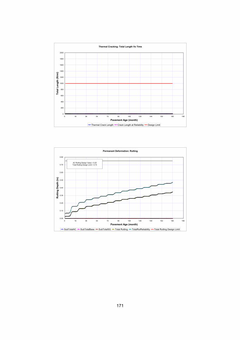
171
Thermal Cracking: Total Length Vs Time
0
200
400
600
800
1000
1200
1400
1600
1800
2000
0 18 36 54 72 90 108 126 144 162 180 198
Pavement Age (month)
Tota
l Len
gth
(ft/m
i)
Thermal Crack Length Crack Length at Reliability Design Limit
Permanant Deformation: Rutting
0.00
0.10
0.20
0.30
0.40
0.50
0.60
0.70
0.80
0 18 36 54 72 90 108 126 144 162 180 198
Pavement Age (month)
Rut
ting
Dep
th (i
n)
SubTotalAC SubTotalBase SubTotalSG Total Rutting TotalRutReliability Total Rutting Design Limit
AC Rutting Design Value = 0.25Total Rutting Design Limit = 0.75
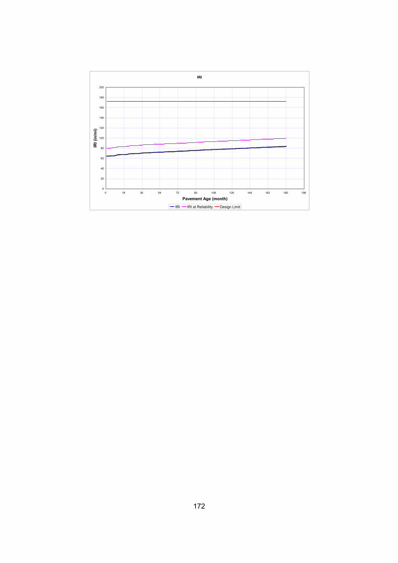
172
IRI
0
20
40
60
80
100
120
140
160
180
200
0 18 36 54 72 90 108 126 144 162 180 198
Pavement Age (month)
IRI (
in/m
i)
IRI IRI at Reliability Design Limit

173
Limit Reliability63
172 9010 90
25754
507060
Class 4 Class 5 Class 6 Class 7 Class 8 Class 9 Class 10 Class 11 Class 12 Class 131.00 1.00 1.00 1.00 1.00 1.00 1.00 1.00 1.00 1.00 1.00 1.00 1.00 1.00 1.00 1.00 1.00 1.00 1.00 1.00 1.00 1.00 1.00 1.00 1.00 1.00 1.00 1.00 1.00 1.00 1.00 1.00 1.00 1.00 1.00 1.00 1.00 1.00 1.00 1.00 1.00 1.00 1.00 1.00 1.00 1.00 1.00 1.00 1.00 1.00 1.00 1.00 1.00 1.00 1.00 1.00 1.00 1.00 1.00 1.00 1.00 1.00 1.00 1.00 1.00 1.00 1.00 1.00 1.00 1.00 1.00 1.00 1.00 1.00 1.00 1.00 1.00 1.00 1.00 1.00 1.00 1.00 1.00 1.00 1.00 1.00 1.00 1.00 1.00 1.00 1.00 1.00 1.00 1.00 1.00 1.00 1.00 1.00 1.00 1.00 1.00 1.00 1.00 1.00 1.00 1.00 1.00 1.00 1.00 1.00 1.00 1.00 1.00 1.00 1.00 1.00 1.00 1.00 1.00 1.00
Midnight 2.3% Noon 5.9%1.3% 1:00 am 2.3% 1:00 pm 5.9%8.5% 2:00 am 2.3% 2:00 pm 5.9%2.8% 3:00 am 2.3% 3:00 pm 5.9%0.3% 4:00 am 2.3% 4:00 pm 4.6%7.6% 5:00 am 2.3% 5:00 pm 4.6%
74.0% 6:00 am 5.0% 6:00 pm 4.6%1.2% 7:00 am 5.0% 7:00 pm 4.6%3.4% 8:00 am 5.0% 8:00 pm 3.1%0.6% 9:00 am 5.0% 9:00 pm 3.1%0.3% 10:00 am 5.9% 10:00 pm 3.1%
11:00 am 5.9% 11:00 pm 3.1%Class 13
Class 9Class 10Class 11Class 12
Class 5Class 6Class 7Class 8
(Level 3, Default Distribution) by period beginning:AADTT distribution by vehicle classClass 4
NovemberDecember
Vehicle Class Distribution Hourly truck traffic distribution
JulyAugustSeptemberOctober
MarchAprilMayJune
Vehicle ClassMonth
JanuaryFebruary
Percent of trucks in design lane (%):Operational speed (mph):
Traffic -- Volume Adjustment FactorsMonthly Adjustment Factors (Level 3, Default MAF)
Traffic Initial two-way aadtt:Number of lanes in design direction:Percent of trucks in design direction (%):
Traffic direction: South bound
Default Input LevelDefault input level Level 3, Default and historical agency values.
Station/milepost begin: 9.52Station/milepost end: 10.02
Station/milepost format: Miles: 0.000
Principal Arterials - Interstate and Defense RoutesDate: 3/1/2005
Project ID: SITE10Section ID:
Terminal IRI (in/mi)CRCP Punchouts (per mi)
Location: Hanover, VA
Analysis type Probabilistic
Performance CriteriaInitial IRI (in/mi)
Type of design CRCP
Analysis Parameters
Project: SITE10-New Design.dgp
General Information Description:o Route: 295 South o County: Hanover (number 42) o Length: 2640 ft o Number of lanes in each direction: 4 o Pavement Category: Composite CRCP older than 20 years w/ surface less than 10 years old o Traffic: TT 3,300 & 3,060, AADT 37,000 & 34,000 o AC Overlay:4in CRCP:8in CTA:6in o Subgrade: silty clay w/fine gravel
Design Life 20 yearsPavement construction: September, 1980Traffic open: October, 1980

174
4.0%4.0%4.0%4.0%4.0%4.0%4.0%4.0%4.0%4.0%
18
1012
1.62 0.39 0.00 0.00 2.00 0.00 0.00 0.00 1.02 0.99 0.00 0.00 1.00 0.26 0.83 0.00 2.38 0.67 0.00 0.00 1.13 1.93 0.00 0.00 1.19 1.09 0.89 0.00 4.29 0.26 0.06 0.00 3.52 1.14 0.06 0.00 2.15 2.13 0.35 0.00
8.5
12
120120
51.649.249.2
Short Medium Long12 15 18
33% 33% 34%
37.77-77.37206917
-10Asphalt
0.7Percent steel (%):
Structure--Design Features Permanent curl/warp effective temperature difference (°F):Shoulder type:
Steel Reinforcement
Latitude (degrees.minutes)Longitude (degrees.minutes)Elevation (ft)Depth of water table (ft)
Climate icm file:
site10-01
Quad axle(psi):
Wheelbase Truck Tractor
Average Axle Spacing (ft)Percent of trucks
Dual Tire (psi):
Average Axle SpacingTandem axle(psi):Tridem axle(psi):
Average axle width (edge-to-edge) outside dimensions,ft):Dual tire spacing (in):
Axle ConfigurationSingle Tire (psi):
Class 11Class 12Class 13
Axle Configuration
Class 7Class 8Class 9Class 10
Quad Axle
Class 4Class 5Class 6
Vehicle Class
Single Axle
Tandem Axle
Tridem Axle
Mean wheel location (inches from the lane marking):Traffic wander standard deviation (in):Design lane width (ft):
Number of Axles per Truck
Traffic -- Axle Load Distribution FactorsLevel 3: Default
Traffic -- General Traffic Inputs
Class 12 CompoundClass 13 Compound
Class 10 CompoundClass 11 Compound
Class 8 CompoundClass 9 Compound
Class 6 CompoundClass 7 Compound
Class 4 CompoundClass 5 Compound
Traffic Growth Factor
Vehicle Class
Growth Rate
GrowthFunction

175
0.85
Modulus (input) (psi): 50000
Poisson's ratio: 0.35Coefficient of lateral pressure,Ko: 0.5
Strength PropertiesInput Level: Level 3Analysis Type: ICM inputs (ICM Calculated Modulus)
Layer 3 -- CLUnbound Material: CLThickness(in): 12
Thermal PropertiesThermal conductivity (BTU/hr-ft-F°) : 1.25Heat capacity (BTU/lb-F°): 0.28
Poisson's ratio: 0.2
Strength PropertiesElastic/resilient modulus (psi): 540000
Layer thickness (in): 6Unit weight (pcf): 150
Layer 2 -- Cement StabilizedGeneral Properties
Material type: Cement Stabilized
28-day PCC modulus of rupture (psi): n/a28-day PCC compressive strength (psi): 3632
Curing method: Curing compound
Strength PropertiesInput level: Level 3
Reversible shrinkage (% of ultimate shrinkage): 50Time to develop 50% of ultimate shrinkage (days): 35
PCC zero-stress temperature (F°) DerivedUltimate shrinkage at 40% R.H (microstrain) Derived
Water/cement ratio: 0.42Aggregate type: Limestone
Mix PropertiesCement type: Type IICementitious material content (lb/yd^3): 564
Thermal conductivity (BTU/hr-ft-F°) : 1.25Heat capacity (BTU/lb-F°): 0.28
Poisson's ratio 0.2
Thermal PropertiesCoefficient of thermal expansion (per F° x 10- 6): 5.5
Layer thickness (in): 8Unit weight (pcf): 150
Structure--Layers Layer 1 -- CRCP
General PropertiesPCC material CRCP
Drainage path length (ft): 12Pavement cross slope (%): 2
Structure--ICM PropertiesSurface shortwave absorptivity:
Drainage ParametersInfiltration: Minor (10%)
Base/slab friction coefficient: 4
Crack SpacingCracking Model Generate using model.
Base type: Cement treatedErodibility index: Fairly Erodable (4)
Base Properties

176
Value68.11.15
0.6582720
Value68.11.15
0.6582720
21.22
105.26324
-0.38158
PunchoutC3C4C5
PunchoutsFatigue
C1C2
bc
Hr.
Distress Model Calibration Settings - Rigid (new)
Soil water characteristic curve parameters: Default values
Parametersa
Optimum gravimetric water content (%): 18.6 (derived)Calculated degree of saturation (%): 87.6 (calculated)
Specific gravity of solids, Gs: 2.73 (derived)Saturated hydraulic conductivity (ft/hr): 3.2175e-005 (derived)
D60 (mm): 0.1
Calculated/Derived ParametersMaximum dry unit weight (pcf): 107.9 (derived)
Passing #200 sieve (%): 75Passing #4 sieve (%): 95
ICM InputsGradation and Plasticity IndexPlasticity Index, PI: 15
Coefficient of lateral pressure,Ko: 0.5Modulus (input) (psi): 50000
Analysis Type: ICM inputs (ICM Calculated Modulus)Poisson's ratio: 0.35
Thickness(in): Semi-infinite
Strength PropertiesInput Level: Level 3
Hr.
Layer 4 -- CLUnbound Material: CL
Parametersabc
Calculated degree of saturation (%): 87.6 (calculated)
Soil water characteristic curve parameters: Default values
Saturated hydraulic conductivity (ft/hr): 3.25e-005 (derived)Optimum gravimetric water content (%): 18.6 (derived)
Calculated/Derived ParametersMaximum dry unit weight (pcf): 107.9 (derived)Specific gravity of solids, Gs: 2.73 (derived)
Passing #4 sieve (%): 95D60 (mm): 0.1
Plasticity Index, PI: 15Passing #200 sieve (%): 75
ICM InputsGradation and Plasticity Index

177
1
13.15
28.3510.03
5.4
C3C4Standard deviation in initial IRI (in/mile):
4.04*POWER(PO, 0.3825)
IRI(crcp)C1C2
Crack WidthC6
Reliability (PO)Std. Dev.
Distress Target
Reliablity Target
Distress Predicted
Reliability Predicted Acceptable
172 90 89.2 99.54 Pass10 90 12.6 40.28 FailCRCP Punchouts (per mi)
Project: SITE10-New Design.dgpReliability Summary
Performance Criteria
Terminal IRI (in/mi)
Predicted Punchout
0.0
2.7
5.3
8.0
10.6
13.3
15.9
18.6
21.2
23.9
26.5
0 2 4 6 8 10 12 14 16 18 20 22
Pavement age, years
Punc
hout
per
mile
Punchout Punchout at specified reliability Punchout Limit

178
IRI
0
18
36
54
72
90
108
126
144
162
180
0 2 4 6 8 10 12 14 16 18 20 22 24
Pavement age, years
IRI,
in/m
ile
IRI IRI at specified reliability IRI Limit

179
Limit Reliability63
172 901000 90
25 901000 90
25 900.25 900.75 90
48234
507060
Class 4 Class 5 Class 6 Class 7 Class 8 Class 9 Class 10 Class 11 Class 12 Class 131.00 1.00 1.00 1.00 1.00 1.00 1.00 1.00 1.00 1.00 1.00 1.00 1.00 1.00 1.00 1.00 1.00 1.00 1.00 1.00 1.00 1.00 1.00 1.00 1.00 1.00 1.00 1.00 1.00 1.00 1.00 1.00 1.00 1.00 1.00 1.00 1.00 1.00 1.00 1.00 1.00 1.00 1.00 1.00 1.00 1.00 1.00 1.00 1.00 1.00 1.00 1.00 1.00 1.00 1.00 1.00 1.00 1.00 1.00 1.00 1.00 1.00 1.00 1.00 1.00 1.00 1.00 1.00 1.00 1.00 1.00 1.00 1.00 1.00 1.00 1.00 1.00 1.00 1.00 1.00 1.00 1.00 1.00 1.00 1.00 1.00 1.00 1.00 1.00 1.00 1.00 1.00 1.00 1.00 1.00 1.00 1.00 1.00 1.00 1.00 1.00 1.00 1.00 1.00 1.00 1.00 1.00 1.00 1.00 1.00 1.00 1.00 1.00 1.00 1.00 1.00 1.00 1.00 1.00 1.00
Midnight 2.3% Noon 5.9%1.3% 1:00 am 2.3% 1:00 pm 5.9%8.5% 2:00 am 2.3% 2:00 pm 5.9%2.8% 3:00 am 2.3% 3:00 pm 5.9%0.3% 4:00 am 2.3% 4:00 pm 4.6%7.6% 5:00 am 2.3% 5:00 pm 4.6%
74.0% 6:00 am 5.0% 6:00 pm 4.6%1.2% 7:00 am 5.0% 7:00 pm 4.6%3.4% 8:00 am 5.0% 8:00 pm 3.1%0.6% 9:00 am 5.0% 9:00 pm 3.1%
Project: SITE10-Rehabilitation.dgp
General Information Description:o Route: 295 South o County: Hanover (number 42) o Length: 2640 ft o Number of lanes in each direction: 4 o Pavement Category: Composite CRCP older than 20 years w/ surface less than 10 years old o Traffic: TT 3,300 & 3,060, AADT 37,000 & 34,000 o AC Overlay:4in CRCP:8in CTA:6in o Subgrade: silty clay w/fine gravel
Design Life 20 yearsExisting pavement construction: September, 1980Pavement overlay construction: September, 1996Traffic open: October, 1996Type of design Flexible
Analysis ParametersAnalysis type Probabilistic
Performance CriteriaInitial IRI (in/mi)Terminal IRI (in/mi)AC Surface Down Cracking (Long. Cracking) (ft/500):AC Bottom Up Cracking (Alligator Cracking) (%):AC Thermal Fracture (Transverse Cracking) (ft/mi):Chemically Stabilized Layer (Fatigue Fracture)Permanent Deformation (AC Only) (in):Permanent Deformation (Total Pavement) (in):
Location: Hanover, VAProject ID: SITE10Section ID:
Principal Arterials - Interstate and Defense RoutesDate: 3/1/2005
Station/milepost format: Miles: 0.000Station/milepost begin: 9.52Station/milepost end: 10.02Traffic direction: South bound
Default Input LevelDefault input level Level 3, Default and historical agency values.
Traffic Initial two-way aadtt:Number of lanes in design direction:Percent of trucks in design direction (%):Percent of trucks in design lane (%):Operational speed (mph):
Traffic -- Volume Adjustment FactorsMonthly Adjustment Factors (Level 3, Default MAF)
Vehicle ClassMonth
JanuaryFebruaryMarchAprilMayJuneJulyAugustSeptemberOctoberNovemberDecember
Vehicle Class Distribution Hourly truck traffic distribution(Level 3, Default Distribution) by period beginning:
AADTT distribution by vehicle classClass 4Class 5Class 6Class 7Class 8Class 9Class 10Class 11Class 12

180
4.0%4.0%4.0%4.0%4.0%4.0%4.0%4.0%4.0%4.0%
18
1012
1.62 0.39 0.00 0.00 2.00 0.00 0.00 0.00 1.02 0.99 0.00 0.00 1.00 0.26 0.83 0.00 2.38 0.67 0.00 0.00 1.13 1.93 0.00 0.00 1.19 1.09 0.89 0.00 4.29 0.26 0.06 0.00 3.52 1.14 0.06 0.00 2.15 2.13 0.35 0.00
8.5
12
120120
51.649.249.2
37.77-77.37206917
-10Asphalt
0.70.6254
Traffic Growth Factor
Vehicle Class
Growth Rate
GrowthFunction
Class 4 CompoundClass 5 CompoundClass 6 CompoundClass 7 CompoundClass 8 CompoundClass 9 CompoundClass 10 CompoundClass 11 CompoundClass 12 CompoundClass 13 Compound
Traffic -- Axle Load Distribution FactorsLevel 3: Default
Traffic -- General Traffic InputsMean wheel location (inches from the lane marking):Traffic wander standard deviation (in):Design lane width (ft):
Number of Axles per Truck
Quad Axle
Class 4Class 5Class 6
Vehicle Class
Single Axle
Tandem Axle
Tridem Axle
Class 7Class 8Class 9Class 10Class 11Class 12Class 13
Axle ConfigurationAverage axle width (edge-to-edge) outside dimensions,ft):Dual tire spacing (in):
Axle ConfigurationSingle Tire (psi):Dual Tire (psi):
Average Axle SpacingTandem axle(psi):Tridem axle(psi):Quad axle(psi):
Climate icm file:
site10-02Latitude (degrees.minutes)Longitude (degrees.minutes)Elevation (ft)Depth of water table (ft)
Structure--Design Features Permanent curl/warp effective temperature difference (°F):Shoulder type:
Steel ReinforcementPercent steel (%):Bar diameter (in):Steel depth (in):
Base PropertiesBase type: Cement treated

181
0.85
Crack SpacingCracking Model Generate using model.
Structure--ICM PropertiesSurface shortwave absorptivity:
Drainage ParametersInfiltration: Minor (10%)Drainage path length (ft): 12Pavement cross slope (%): 2
Structure--Layers Layer 1 -- Asphalt concrete
Material type: Asphalt concreteLayer thickness (in): 4
General PropertiesGeneralReference temperature (F°): 70
Volumetric Properties as BuiltEffective binder content (%): 6Air voids (%): 4Total unit weight (pcf): 148
Poisson's ratio: 0.35 (user entered)
Thermal PropertiesThermal conductivity asphalt (BTU/hr-ft-F°): 0.67Heat capacity asphalt (BTU/lb-F°): 0.23
Asphalt MixCumulative % Retained 3/4 inch sieve: 0Cumulative % Retained 3/8 inch sieve: 38Cumulative % Retained #4 sieve: 75% Passing #200 sieve: 10
Asphalt BinderOption: Conventional viscosity gradeViscosity Grade AC 20A 10.7709 (correlated)VTS: -3.6017 (correlated)
Layer 2 -- CRCP (existing)General Properties
PCC material CRCP (existing)Layer thickness (in): 8Unit weight (pcf): 150Poisson's ratio 0.2
Thermal PropertiesCoefficient of thermal expansion (per F° x 10- 6): 5.5Thermal conductivity (BTU/hr-ft-F°) : 1.25Heat capacity (BTU/lb-F°): 0.28
Mix PropertiesCement type: Type IICementitious material content (lb/yd^3): 564Water/cement ratio: 0.45Aggregate type: LimestonePCC zero-stress temperature (F°) DerivedUltimate shrinkage at 40% R.H (microstrain) DerivedReversible shrinkage (% of ultimate shrinkage): 50Time to develop 50% of ultimate shrinkage (days): 35Curing method: Curing compound
Strength PropertiesInput level: Level 328-day PCC modulus of rupture (psi): n/a28-day PCC compressive strength (psi): 3632

182
Value68.11.15
0.6582720
Layer 3 -- Cement StabilizedGeneral Properties
Material type: Cement StabilizedLayer thickness (in): 6Unit weight (pcf): 150Poisson's ratio: 0.2
Strength PropertiesElastic/resilient modulus (psi): 540000
Thermal PropertiesThermal conductivity (BTU/hr-ft-F°) : 1.25Heat capacity (BTU/lb-F°): 0.28
Layer 4 -- CLUnbound Material: CLThickness(in): 12
Strength PropertiesInput Level: Level 3Analysis Type: ICM inputs (ICM Calculated Modulus)Poisson's ratio: 0.35Coefficient of lateral pressure,Ko: 0.5Modulus (input) (psi): 50000
ICM InputsGradation and Plasticity IndexPlasticity Index, PI: 15Passing #200 sieve (%): 75Passing #4 sieve (%): 95D60 (mm): 0.1
Calculated/Derived ParametersMaximum dry unit weight (pcf): 107.9 (derived)Specific gravity of solids, Gs: 2.73 (derived)Saturated hydraulic conductivity (ft/hr): 3.25e-005 (derived)Optimum gravimetric water content (%): 18.6 (derived)Calculated degree of saturation (%): 87.6 (calculated)
Soil water characteristic curve parameters: Default values
Parametersabc
Hr.
Layer 5 -- CLUnbound Material: CLThickness(in): Semi-infinite
Strength PropertiesInput Level: Level 3Analysis Type: ICM inputs (ICM Calculated Modulus)Poisson's ratio: 0.35Coefficient of lateral pressure,Ko: 0.5Modulus (input) (psi): 50000
ICM InputsGradation and Plasticity IndexPlasticity Index, PI: 15Passing #200 sieve (%): 75Passing #4 sieve (%): 95D60 (mm): 0.1
Calculated/Derived ParametersMaximum dry unit weight (pcf): 107.9 (derived)Specific gravity of solids, Gs: 2.73 (derived)Saturated hydraulic conductivity (ft/hr): 3.2175e-005 (derived)Optimum gravimetric water content (%): 18.6 (derived)Calculated degree of saturation (%): 87.6 (calculated)
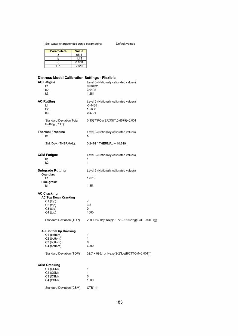
183
Value68.11.15
0.6582720
0.004323.94921.281
-3.44881.56060.4791
5
11
1.673
1.35
73.501000
1106000
1101000
Soil water characteristic curve parameters: Default values
Parametersabc
Hr.
Distress Model Calibration Settings - Flexible AC Fatigue Level 3 (Nationally calibrated values)
k1k2k3
AC Rutting Level 3 (Nationally calibrated values)k1k2k3
Standard Deviation Total Rutting (RUT):
0.1587*POWER(RUT,0.4579)+0.001
Thermal Fracture Level 3 (Nationally calibrated values)k1
Std. Dev. (THERMAL): 0.2474 * THERMAL + 10.619
CSM Fatigue Level 3 (Nationally calibrated values)k1k2
Subgrade Rutting Level 3 (Nationally calibrated values)Granular:
k1Fine-grain:
k1
AC CrackingAC Top Down Cracking
C1 (top)C2 (top)C3 (top)C4 (top)
Standard Deviation (TOP) 200 + 2300/(1+exp(1.072-2.1654*log(TOP+0.0001)))
AC Bottom Up CrackingC1 (bottom)C2 (bottom)C3 (bottom)C4 (bottom)
Standard Deviation (TOP) 32.7 + 995.1 /(1+exp(2-2*log(BOTTOM+0.001)))
CSM CrackingC1 (CSM)C2 (CSM)C3 (CSM)C4 (CSM)
Standard Deviation (CSM) CTB*11

184
0.0115050.0035993.4300570.0007230.0112419.042440.179
0.0082630.0221831.330410.197
IRIIRI Rehabilitation over Flexible
C1 (Flexible)C2 (Flexible)C3 (Flexible)C4 (Flexible)C5 (Flexible)C6 (Flexible)
C3 (Rigid)Std. Dev (Rigid)
Std. Dev (Flexible)
IRI Rehabilitation over RigidC1 (Rigid)C2 (Rigid)
Distress Target
Reliablity Target
Distress Predicted
Reliability Predicted Acceptable
172 90 99 99.999 Pass
1000 90 0 99.999 Pass
25 90 0 99.999 Pass
1000 90 1 99.999 Pass25 90 N/A
0.25 90 0.71 0.04 Fail0.75 90 0.71 62.48 Fail
Project: SITE10-Rehabilitation.dgpReliability Summary
Performance Criteria
Terminal IRI (in/mi)
Permanent Deformation (AC Only) (in):Permanent Deformation (Total Pavement) (in):
AC Surface Down Cracking (Long. Cracking) (ft/500):AC Bottom Up Cracking (Alligator Cracking) (%):AC Thermal Fracture (Transverse Cracking) (ft/mi):Chemically Stabilized Layer (Fatigue Fracture)

185
Asphalt Sub-Layers Modulus Vs Time
0
500,000
1,000,000
1,500,000
2,000,000
2,500,000
3,000,000
3,500,000
4,000,000
4,500,000
0 24 48 72 96 120 144 168 192 216 240
Pavement Age (month)
Mod
ulus
(psi
)
AC1(1) h=0.5 AC1(2) h=0.5 AC1(3) h=1.0 AC1(4) h=1.0 AC1(5) h=1.0
Surface Down Cracking - Longitudinal
0
200
400
600
800
1000
1200
1400
1600
1800
2000
0 24 48 72 96 120 144 168 192 216 240 264
Pavement Age (month)
Long
itudi
nal C
rack
ing
(ft/m
i)
Surface Depth = 0.5" Surface at Reliability Design Limit

186
Bottom Up Cracking - Alligator
0
10
20
30
40
50
60
70
80
90
100
0 24 48 72 96 120 144 168 192 216 240 264
Pavement Age (month)
Alli
gato
r Cra
ckin
g (%
)
Maximum Cracking Bottom Up Reliability Maximum Cracking Limit
Thermal Cracking: Total Length Vs Time
0
200
400
600
800
1000
1200
1400
1600
1800
2000
0 24 48 72 96 120 144 168 192 216 240 264
Pavement Age (month)
Tota
l Len
gth
(ft/m
i)
Thermal Crack Length Crack Length at Reliability Design Limit

187
Permanant Deformation: Rutting
0.00
0.10
0.20
0.30
0.40
0.50
0.60
0.70
0.80
0.90
1.00
0 24 48 72 96 120 144 168 192 216 240 264
Pavement Age (month)
Rut
ting
Dep
th (i
n)
SubTotalAC SubTotalBase SubTotalSG Total Rutting TotalRutReliability Total Rutting Design Limit
AC Rutting Design Value = 0.25Total Rutting Design Limit = 0.75
IRI
0
20
40
60
80
100
120
140
160
180
200
0 24 48 72 96 120 144 168 192 216 240 264
Pavement Age (month)
IRI (
in/m
i)
IRI IRI at Reliability Design Limit

188
VITA
Carlos Gramajo was born in Guatemala City, Guatemala. In July 2002 he received his degree of
Bachelor of Science in Civil Engineering at Universidad del Valle, Guatemala. He started
working as a design engineer in a consulting company called CM Ingenieros in Guatemala, from
July 2002 to August 2003. During this time, his work involved basically the analysis of Non-
Destructive Evaluation measurements performed with Falling Weight Deflectometer and Surface
Profilemeter; he was also involved in the structural design of different new and rehabilitated
highways in his country. In August 2003, he started his M.S. program at Virginia Tech
Polytechnic Institute and State University, Blacksburg, Virginia, joining the Transportation
Infrastructure and Systems Engineering program under the supervision of Dr. Gerardo Flintsch.