verification and validation of rural propagation in the ... · pdf fileverification and...
TRANSCRIPT
ARL-TR-7745 ● AUG 2016
US Army Research Laboratory
Verification and Validation of Rural Propagation in the Sage 2.0 Simulation by Jayashree Harikumar, Patrick Honan, Jesse Jackman, Brad Morgan, and Lon Anderson Approved for public release; distribution unlimited.
NOTICES
Disclaimers
The findings in this report are not to be construed as an official Department of the Army position unless so designated by other authorized documents.
Citation of manufacturer’s or trade names does not constitute an official endorsement or approval of the use thereof.
Destroy this report when it is no longer needed. Do not return it to the originator.
ARL-TR-7745 ● AUG 2016
US Army Research Laboratory
Verification and Validation of Rural Propagation in the Sage 2.0 Simulation by Lon Anderson Survivability/Lethality Analysis Directorate, ARL Jayashree Harikumar, Patrick Honan, Jesse Jackman, and Brad Morgan Physical Science Laboratory (PSL) New Mexico State University, Las Cruces, NM Approved for public release; distributon unlimited.

ii
REPORT DOCUMENTATION PAGE Form Approved OMB No. 0704-0188
Public reporting burden for this collection of information is estimated to average 1 hour per response, including the time for reviewing instructions, searching existing data sources, gathering and maintaining the data needed, and completing and reviewing the collection information. Send comments regarding this burden estimate or any other aspect of this collection of information, including suggestions for reducing the burden, to Department of Defense, Washington Headquarters Services, Directorate for Information Operations and Reports (0704-0188), 1215 Jefferson Davis Highway, Suite 1204, Arlington, VA 22202-4302. Respondents should be aware that notwithstanding any other provision of law, no person shall be subject to any penalty for failing to comply with a collection of information if it does not display a currently valid OMB control number. PLEASE DO NOT RETURN YOUR FORM TO THE ABOVE ADDRESS.
1. REPORT DATE (DD-MM-YYYY)
August 2016 2. REPORT TYPE
Technical Report 3. DATES COVERED (From - To)
01/2013–05/2013 4. TITLE AND SUBTITLE
Verification and Validation of Rural Propagation in the Sage 2.0 Simulation 5a. CONTRACT NUMBER
5b. GRANT NUMBER
5c. PROGRAM ELEMENT NUMBER
6. AUTHOR(S)
Jayashree Harikumar, Patrick Honan, Jesse Jackman, Brad Morgan, and Lon Anderson
5d. PROJECT NUMBER
5e. TASK NUMBER
5f. WORK UNIT NUMBER
7. PERFORMING ORGANIZATION NAME(S) AND ADDRESS(ES)
US Army Research Laboratory Cybersecurity and Electromagnetic Protection Division Survivability/Lethality Analysis Directorate ATTN: RDRL-SLE-M White Sands Missile Range, NM 88005-5513
8. PERFORMING ORGANIZATION REPORT NUMBER
ARL-TR-7745
9. SPONSORING/MONITORING AGENCY NAME(S) AND ADDRESS(ES)
10. SPONSOR/MONITOR'S ACRONYM(S)
11. SPONSOR/MONITOR'S REPORT NUMBER(S)
12. DISTRIBUTION/AVAILABILITY STATEMENT
Approved for public release; distribution unlimited.
13. SUPPLEMENTARY NOTES
14. ABSTRACT
The purpose of this report is to provide Verification and Validation of the Sage 2.0 rural propagation prediction features and to establish confidence and usage bounds. These boundaries are defined by the intended use and the constraints, limitations, and assumptions. 15. SUBJECT TERMS
System of Systems, PSL, Physical Science Laboratory, MR1, Major Release 1, S4, System of Systems Survivability Simulation, JTRS-RR, Joint Tactical Radio System-Rifleman Radio, SNR, Signal-to-Noise Ratio, V&V, Verification and Validation
16. SECURITY CLASSIFICATION OF: 17. LIMITATION OF ABSTRACT
UU
18. NUMBER OF PAGES
36
19a. NAME OF RESPONSIBLE PERSON
Kurt L Austin a. REPORT
Unclassified b. ABSTRACT
Unclassified c. THIS PAGE
Unclassified 19b. TELEPHONE NUMBER (Include area code)
(575) 678-1816 Standard Form 298 (Rev. 8/98) Prescribed by ANSI Std. Z39.18

Approved for public release; distribution unlimited. iii
Contents
List of Figures v
List of Tables v
1. Introduction 1
2. Purpose 2
3. Objective 2
4. Intended Use 2
5. Scope 2
6. Constraints, Limitations, and Assumptions 3
6.1 Constraints 3
6.2 Limitations 3
6.3 Assumptions 4
7. Synopsis of V&V Methodology 4
8. Unit-Level Verification Tests for Path Loss, Link Quality, and Noise 6
8.1 Propagation Regression Testing Using DTED Level 1 Terrain 6
8.2 Propagation Regression Testing Using DTED Level 2 Terrain 6
8.3 Link Quality Tests 7
8.4 Noise Unit Tests 8
9. Description of Sage TIREM Implementation and Simulation-Level Tests 8
9.1 TIREM Description and History 8
9.2 Sage Screenshots for Link Comparison 9
9.3 Sage Path Loss 11
9.4 Terrain Modeling 13

Approved for public release; distribution unlimited. iv
9.5 Distance Calculation 13
9.6 Shortest Path 14
9.7 Terrain Interpolation 14
10. Verification of Sage 2.0 Path Loss and SNR at the Simulation Level 15
10.1 Standalone TIREM to Sage TIREM Overall Comparison 16
10.2 SNR Comparisons 17
11. Validation and Error Bounds of TIREM and Data Sources 19
11.1 TIREM V&V and Expected Accuracy 20
11.2 Radio Data Sources 20
11.3 Noise Data Validity 22
12. Conclusions 24
13. References 25
List of Symbols, Abbreviations, and Acronyms 26
Distribution List 27

Approved for public release; distribution unlimited. v
List of Figures
Fig. 1 Screenshot from Global Mapper showing a radio link with parameters: 350 MHzRef3-L0R7000-L179R6000 ..................................................10
Fig. 2 Terrain profile that corresponds to the link shown in Fig. 1 ................10
Fig. 3 Sage screenshot example that demonstrates agreement between Sage path loss and the value produced by the standalone TIREM. The parameters run for this example were transmitter position 320317.64N latitude 1060813.20W longitude; receiver position 320336.73N latitude and 1061433.87W longitude; frequency 1380 MHz; and elevation sample spacing 46.52 m. ......................................................11
Fig. 4 Terrain posts and triangles ...................................................................14
Fig. 5 Comparison of standalone TIREM to Sage TIREM for links with matching terrain profiles ......................................................................15
Fig. 6 Comparison of standalone TIREM to Sage TIREM for links with nearly matching terrain profiles and anomalous events circled ...........16
List of Tables
Table 1 An excerpt from 20130412-RuralProp-Jammer-with Cmp.xlsx ...........7
Table 2 Summary of all tested links..................................................................17
Table 3 Spreadsheet for case with no jammer ..................................................18
Table 4 Further details describing case with no jammer ..................................18
Table 5 Spreadsheet for the jammer case..........................................................19
Table 6 List of data sources for radio parameters .............................................21
Table 7 Characteristics of JTRS-RR and Manpack radio kits ..........................22
Table 8 Computed Rx sensitivity for JTRS-RR and Manpack radios ..............22

Approved for public release; distribution unlimited. vi
INTENTIONALLY LEFT BLANK.
Approved for public release; distribution unlimited. 1
1. Introduction
The System of Systems Survivability Simulation (S4) is designed to be used by analysts of the US Army Research Laboratory’s (ARL’s) Survivability/Lethality Analysis Directorate (SLAD) to investigate survivability, lethality, and vulnerability (SLV) issues in a mission context containing multiple systems. SLAD and the Physical Science Laboratory (PSL) of New Mexico State University (NMSU) are working together to develop S4. A general S4 usage description has been previously published by SLAD.1 Three key areas of SLAD’s SLV mission are supported by S4: Electronic Warfare (including communications systems), Information Operations/Information Warfare, and Ballistics.
As part of the SLV mission involving communications systems, SLAD assesses various potential vulnerabilities in radios and radio networks through laboratory and field investigations, and explores the resulting survivability impacts of these vulnerabilities in a System of Systems mission context using modeling and simulation. The findings of these investigations inform Army decision makers, the Army’s independent evaluator, and materiel developers.
The Sage model, part of the S4 simulation suite, has been developed primarily to support SLAD analysts in pretest planning and quick turnaround analyses of Electronic Warfare/Communications events during field tests. For the verified and validated usage described in this report, Sage is configured to run on an analyst’s personal computer during a field test or laboratory investigation.
The Joint Tactical Radio System (JTRS), a software-defined family of radios, is planned to be the next-generation voice-and-data radio used by the US Military. Several features of the JTRS Rifleman Radio (RR) and Manpack radio are implemented in Sage 2.0; however, it should be stressed that this Verification and Validation (V&V) activity is focused on and limited to rural propagation effects.
The JTRS-RR is intended to enhance situational awareness at the Squad level. According to General Martin Dempsey, Chairman of the Joint Chiefs of Staff, “In assessing our ability to overmatch, we traditionally view the force from the top-down. However, as we build Army 2020, we will begin by looking at the force from the bottom-up with the Squad as the foundation.” SLAD is particularly interested in how JTRS radios and radio-supported mobile ad-hoc networks function, operate, and support Warfighters in both urban and rural environments, especially with regard to SLV issues.

Approved for public release; distribution unlimited. 2
2. Purpose
Our purpose is to document V&V of the Sage 2.0 rural propagation prediction features and to establish confidence and usage bounds. These boundaries are defined by the intended use and the constraints, limitations, and assumptions (CLAs).
3. Objective
The objective is to use a verified and validated model for evaluating SLAD SLV issues that require models of rural propagation effects. V&V is bounded by the conditions described in this report.
4. Intended Use
The intended use of Sage 2.0 is to provide SLAD analysts and their customers a tool for pretest planning and in-test analyses with quick turnaround of results.
Although Sage 2.0 has many useful features that do not require validation for test planning purposes, the only validated use established in this report is the prediction of link quality between radios in both benign and jammer scenarios. In this validated usage, SLAD analysts can optimize relative jammer and radio placements in a rural terrain to analyze jammer effects on link quality. SLAD analysts can also play back GPS coordinates of radio users from an actual test event and analyze radio performance as a function of link quality.
5. Scope
For the purposes of this V&V activity, link quality refers to the signal-to-noise ratio (SNR) of the link between JTRS Rifleman and Manpack Radios in both benign and jamming scenarios. These 2 scenarios are described as follows:
1) Baseline, benign case (no jamming): In this case, we are interested in the SNR of the link between different radio pairings. The radios may be all possible combinations of RR and Manpack at both transmitter and receiver. The link quality for each propagation direction between radios is calculated, and is never assumed to be symmetrical in both directions. The signal part of SNR is derived from transmitter power, transmitter antenna gain, path loss, and receiver antenna gain. Transmitter power, transmitter antenna gain, and receiver antenna gain are derived from RR and Manpack specifications (see Tables 6–8, Section 11). Path loss, the loss between 2
Approved for public release; distribution unlimited. 3
radio nodes, is predicted using the Terrain Integrated Rough Earth Model (TIREM) in Sage. In addition to path loss, we verify the proper implementation of both noise sources internally generated in the radio receiver and ambient radio frequency noise external to the receiver.
2) Jamming case: Jamming is restricted to barrage jamming only, and the noise from the jammer is added to the noise described in the baseline case. The amount of jamming noise power at the radio receiver is derived from jammer power, jammer antenna gain, path loss, and receiver antenna gain. In addition to the path loss between 2 radios, the path loss between jammer(s) and the radio receiver is also computed. The jammer noise is added to the noise calculated in the baseline case.
6. Constraints, Limitations, and Assumptions
CLAs are an important tool for communicating and establishing the bounds of the V&V. For this V&V, we used the Military Operational Research Society’s definitions2 of CLAs:
• Constraint: A restriction imposed by the study sponsor that limits the study team’s options in conducting the study.
• Limitation: An inability of the study team to fully meet the experiment objectives or fully investigate the experiment issues.
• Assumption: 1) An educated supposition in an experiment to replace facts that are not in evidence but are important to the successful completion of a study (contrasted to presumption). 2) Statement related to the study that is taken as true in the absence of facts, often to accommodate a limitation (inclusive of presumptions).
6.1 Constraints
This V&V activity was constrained to be completed in 6 months. The S4 program is following an iterative V&V process, so future model releases will also be V&V’d as they are developed. Also, features within Sage 2.0 that are not V&V’d at this point in time will be V&V’d as time and resource constraints allow.
6.2 Limitations
The Sage 2.0 model met our objectives with one limitation. This limitation is that we did not observe sufficiently close agreement when using the US Military Specification Digital Terrain Elevation Data (DTED), MIL-PRF-89020B,3

Approved for public release; distribution unlimited. 4
standard from National Geospatial-Intelligence Agency 2 terrain data, when it was compared to results using DTED Level 1 terrain data. (Level 1 data has a post spacing of approximately 90 m; Level 2 data has a post spacing of approximately 30 m). Because we were not able to satisfactorily explain the reasons for the differences, we cannot claim validity against all terrain resolution types. For this activity, we are limited to V&V only for DTED Level 1 terrain data. This issue is discussed further in Section 8, in the subsections “Propagation Regression Testing Using DTED Level 1 Terrain” and “Propagation Regression Testing Using DTED Level 2 Terrain”, and in Section 9, in the subsection “Sage Path Loss”.
Limitations should not be confused with error sources in the submodels used in Sage, such as TIREM. These error sources are described in Section 11, “Validation and Error Bounds of TIREM and Data Sources.”
6.3 Assumptions
The primary model used in computing path loss in Sage 2.0 is TIREM. We assume that TIREM is valid within known error bounds for the terrain types that SLAD analysts encounter when Sage 2.0 is used to support a particular test event or study activity.
7. Synopsis of V&V Methodology
Both verification and validation depend on the perspective of intended use. Simplified definitions follow:
• Verification: The process of determining that a model or simulation implementation and its associated data accurately represent the developer’s conceptual description and specifications. Verification is aimed at answering the question, “Did I build the thing right?”.
• Validation: The process of determining the degree to which a model or simulation and its associated data are an accurate representation of the real world from the perspective of the intended uses of the model. Verification is aimed at answering the question, “Did I build the right thing?”.
The governing V&V process and methodology used for this activity were based on the SLAD report, “Verification and Validation (V&V) Methodology for the System of Systems Survivability Simulation (S4),” which was intended to be general enough to support a wide range of V&V activities.4 It is outside the scope of this report to reconstruct the V&V methodology in its entirety, but it is useful to revisit the underlying concepts.
Approved for public release; distribution unlimited. 5
In every model development, choices regarding fidelity and technical focus areas involve human judgment. In the case of S4, these choices are typically made by analysts with SLAD SLV expertise. In addition to bringing the right technical knowledge to bear, this also helps ensure that the modeling choices are made based upon the objectives of the analysts who will ultimately be using the model. The process followed in the S4 project is the creation of domain model specifications (DMS) by SLAD SLV experts. The DMS describe the models that need to be developed, or select an existing model and describe the necessary interfaces to that model. The overall validity of Sage 2.0 for meeting its experimental objectives is determined by the sufficiency of this process and the expertise of the subject matter experts who create the DMS.
In addition to the overall validity of Sage 2.0 as developed by the SLAD SLV experts, we are also interested in the validity of the submodels used in Sage 2.0. For this V&V activity, we are especially interested in the validity of TIREM for path loss, and the validity of the data used to compute SNR.
The DMS, in turn, are used by software developers to create software model specifications (SMS) that translate the DMS into terminology that can be turned into software code. A critical next step is a review involving both domain-level experts and software experts, to ensure that the SMS meet the intent of the DMS.
After the software code is developed, each software requirement is tested in a unit test. SMS incorporate 2 methods for programmatic verification of requirements: unit tests and sim-health reports. All nontrivial requirements have one or more of such verification tests. These tests are employed throughout the development cycle, as well as used for verifying the final release of the product.
Unit tests are used to test model implementations in isolation, from other models as well as from specific scenarios. They are used for verification in the V&V process and for regression testing. These regression tests are not only used within the development cycle but may live well past the life of the major release.
Sim-health reports take data from a set of simulation runs and inspect that data to ensure that the models obey various constraints. In the context of verification, constraints specified in the software requirements are compared to what is observed in the run-set. If the sim-health report passes, it means that for all runs, the models obeyed the tested constraints. If the models exceed the constraints, the report fails and those instances are identified.
Unit tests and sim-health reports are covered in Section 8, “Unit Level Verification Tests for Path Loss, Link Quality, and Noise.”

Approved for public release; distribution unlimited. 6
After unit test and sim-health reports are completed, the SLV analyst runs simulation-level tests to verify that the simulation is performing as intended. For this V&V activity, these higher level tests were fairly simple and straightforward, and the analysts were able to check simulation results against standalone models and spreadsheets. Simulation-level tests are covered in Section 10, “Verification of Sage 2.0 Path Loss and SNR at the Simulation Level.”
The final step in the verification process is to trace from tests to SMS to DMS to ensure that all domain requirements are addressed.
8. Unit-Level Verification Tests for Path Loss, Link Quality, and Noise
The following 4 unit tests provide results and details for each testing area, as well as important references.
8.1 Propagation Regression Testing Using DTED Level 1 Terrain
This test is based on a large set of coordinates that were run in a standalone TIREM and compared to the same coordinates/terrain in Sage 2.0.5 The test passed with all links, no recalculations, and no duplications, because the values of standard deviation and mean are within the limits defined by the domain expert. The differences between the standalone model and the Sage model are standard deviation: 0.7 dB; mean: 0.006 dB.
8.2 Propagation Regression Testing Using DTED Level 2 Terrain
This test is based on a large set of coordinates that were run in Sage 2.0 using DTED 2 terrain, and compared to the same coordinates, but using DTED 1 terrain, in the standalone TIREM.5 The test failed, because the values of standard deviation and mean were not within the limits defined by the domain expert. We expected the test to fail in standard deviation, because the DTED Level 2 is higher resolution and one would expect different TIREM results. However, we were surprised to find that the test failed in the comparison of mean values. The differences between the standalone model and the Sage model are standard deviation: 6.0 dB; mean: 7.3 dB.
Upon examination of the DTED Level 2 terrain data, we discovered several dropouts where terrain data was nonexistent. Upon visual examination, the terrain also contained odd patterns. However, the reason that this set of data produced such a large difference in mean values has not yet been fully run to ground. It has not been adequately proven that the fault lies with the DTED Level 2 data. It could also be that the DTED Level 1 data is producing the errors. However, we chose to use
Approved for public release; distribution unlimited. 7
the DTED Level 1 terrain data for Sage 2.0 at this time because the combination of DTED Level 1 terrain data with TIREM has been used in another V&V’d model, the Network Connectivity Analysis Model (NCAM).6 The last possibility is that TIREM simply produces different results for different terrain resolutions, which can only ultimately be resolved through comparison of Sage 2.0 with actual TIREM-measured validation data.
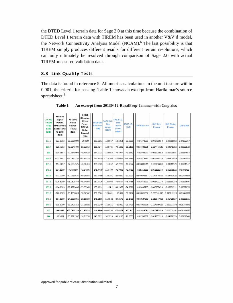
8.3 Link Quality Tests
The data is found in reference 5. All metrics calculations in the unit test are within 0.001, the criteria for passing. Table 1 shows an excerpt from Harikumar’s source spreadsheet.5
Table 1 An excerpt from 20130412-RuralProp-Jammer-with Cmp.xlsx
Approved for public release; distribution unlimited. 8
8.4 Noise Unit Tests
The tests passed as follows:
1) For the noise model test, there are 2 asserts for each link. One checks the nonjammer (environmental) noise in the spreadsheet against what is computed by the model, and the difference was within 0.001 dB.
2) The other assert checks that the total noise power from the spreadsheet (based on TIREM propagation) agrees to that computed by the noise model to within 0.1 dB.
9. Description of Sage TIREM Implementation and Simulation-Level Tests
The following checks were made at the Sage simulation level:
• Requirements specified in the domain document were checked for content.
• CLAs were reviewed.
• Software specifications developed from the domain model requirements were verified for consistency with the domain specifications.
• Results from unit tests matched expected results in standalone calculations and spreadsheets.
• Standalone TIREM was compared to Sage TIREM.
9.1 TIREM Description and History
TIREM is a rough earth model. This class of model considers the effects of the irregular terrain (elevation profile) along the propagation path and in the vicinity of the antennas. Many of the concepts and algorithms employed in TIREM were based on work done at the Central Radio Propagation Laboratory of the National Bureau of Standards by Rice, Longley et al. in the late 1960s.7
The Electromagnetic Compatibility Analysis Center (ECAC) was the originator of TIREM8 in a computerized model form, beginning to achieve reasonable maturity as a Fortran program in the early 1980s. Many of the initial efforts were focused on making the code more compact and faster; these issues have since been largely overcome by great improvements in processor speeds and memory size.
SLAD participated in an in-depth measurement program to compare TIREM with measured data. The region around Flagstaff, Arizona, was chosen because it offered
Approved for public release; distribution unlimited. 9
a suitable variety of terrain. SLAD was interested to see whether bandwidth makes a difference in propagation. To do the experiment, SLAD transmitted narrowband and wideband radio waveforms, and varied the location of the transmitter relative to a calibrated receiver. In short, bandwidth did not make a significant difference in propagation. Many cubic meters of 9-track tapes were accumulated and processed. The resultant SLAD data enabled ECAC to modify TIREM for DOD use and eventually led to the creation of a Java version of TIREM (via Alion Science and Technologies) to become the de facto propagation tool for the Federal Government. TIREM is used in hundreds of modeling and simulation (M&S) tools and tactical Military radios for the DOD. This code is the version S4 and NCAM are using. One result of the data analysis was that ECAC (through its contractor IITRI) tweaked TIREM slightly in the mid-1980s.
The ECAC became the Joint Spectrum Center and a new contractor, Alion Science, was used. Alion Science wrote a Java version of the Fortran code. This is the version used in both S4 and NCAM.
9.2 Sage Screenshots for Link Comparison
Figure 1 shows a screen capture from Global Mapper for a random link. Figure 2 shows the terrain profile for the link in Fig. 1. These figures are examples of a typical terrain type and elevation profile from Sage used to compare against standalone TIREM.

Approved for public release; distribution unlimited. 10
Fig. 1 Screenshot from Global Mapper showing a radio link with parameters: 350 MHzRef3-L0R7000-L179R6000
Fig. 2 Terrain profile that corresponds to the link shown in Fig. 1
Approved for public release; distribution unlimited. 11
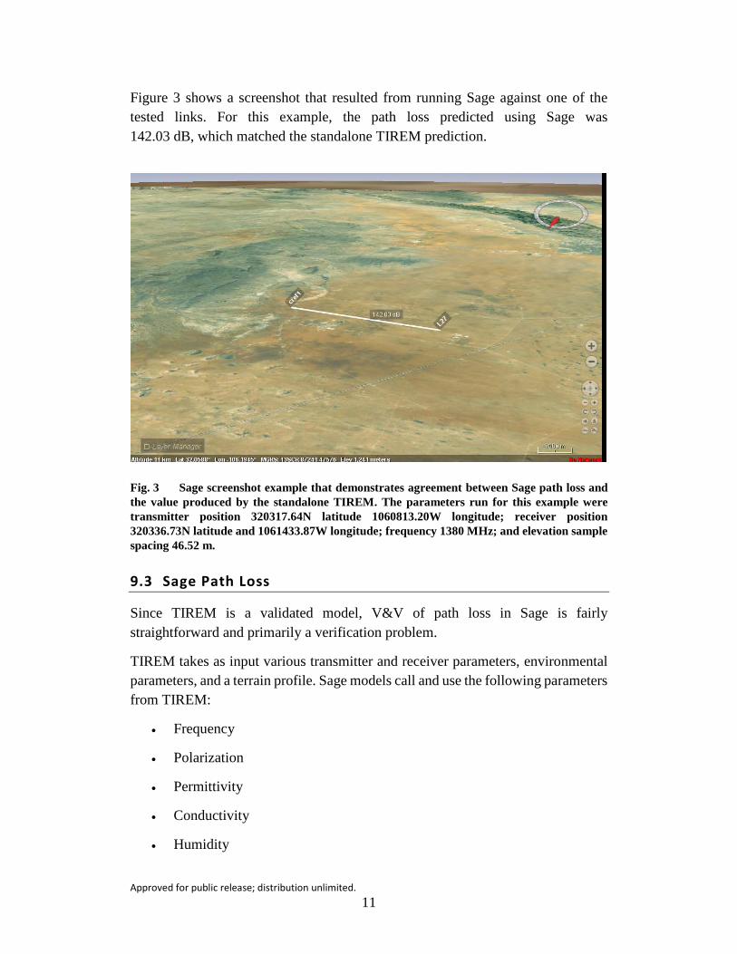
Figure 3 shows a screenshot that resulted from running Sage against one of the tested links. For this example, the path loss predicted using Sage was 142.03 dB, which matched the standalone TIREM prediction.
Fig. 3 Sage screenshot example that demonstrates agreement between Sage path loss and the value produced by the standalone TIREM. The parameters run for this example were transmitter position 320317.64N latitude 1060813.20W longitude; receiver position 320336.73N latitude and 1061433.87W longitude; frequency 1380 MHz; and elevation sample spacing 46.52 m.
9.3 Sage Path Loss
Since TIREM is a validated model, V&V of path loss in Sage is fairly straightforward and primarily a verification problem.
TIREM takes as input various transmitter and receiver parameters, environmental parameters, and a terrain profile. Sage models call and use the following parameters from TIREM:
• Frequency
• Polarization
• Permittivity
• Conductivity
• Humidity
Approved for public release; distribution unlimited. 12
• Refractivity
• Transmitter and receiver antenna height above the ground
Sage was not formally tested against a wide variety of polarization, permittivity, conductivity, humidity, and refractivity values, and the default values in Sage are recommended. The limited testing we did by varying these values did not significantly affect results. We found that for most of our work, the terrain elevation profile is the most important factor contributing to TIREM path-loss calculations (outside of spherical spreading, of course).
Standalone TIREM is a tool that is able to load a terrain dataset in the form of a DTED file, and that allows the user to issue TIREM queries across that terrain. The V&V of Sage’s propagation model was done by issuing a common set of queries against the same terrain data to both the Sage propagation model and to standalone TIREM, and then comparing the output of each.
As mentioned, one of the inputs to TIREM is a terrain profile. The profile is passed to TIREM in the form of a vector of terrain samples, each of which has an associated distance from the transmitter and an elevation (from sea level in meters). The distance is assumed to be “as the crow flies” at sea level. More specifically, distances are measured from some map coordinate to another as if the entire globe were featureless, with all surface elevations being at sea level. Elevations are assumed to be relative to sea level.
Standalone TIREM and the Sage TIREM were both loaded with a DTED 1 dataset with spacing between terrain posts of exactly 3 arc-seconds, or roughly 100 m. Terrain is bounded by latitude 31°, 33° N and longitude 107°, 105° W. TIREM was configured to generate terrain profiles by sampling the terrain at roughly 1.5-arc-second intervals.
Because DTED Level 1 terrain data is fairly coarse, and because the 1.5-arc-second sample interval used by TIREM is close to the 3-arc-second resolution of the terrain data, a slight difference in terrain profile sample spacing can in some cases yield drastically different terrain profiles. Therefore, it was extremely important to replicate the terrain profiling algorithm used by standalone TIREM as closely as possible in Sage. That algorithm is described as follows:
1) D = distance between start and end in meters
2) Dgc = great circle distance between the start and end points in arc-seconds
3) Nintervals = Floor (Dgc / 1.5 arc-seconds)
4) Sample the terrain at d = D * n/Nintervals where n = [0, Nintervals]
Approved for public release; distribution unlimited. 13
We concluded that, for reasons unknown, in many of these cases, the value of Ninterval used by Sage for a query (computed using the algorithm above) differed from the value used by standalone TIREM. Therefore, in cases where the path-loss value computed by Sage differed from that of TIREM by more than 0.5 dB, the offending query was repeated by varying Nintervals by as much as ±3 to find a result that best matched TIREM.
Performing the search produced a much closer match to TIREM, but some anomalies remained. It was found that by adjusting one of the peaks in the elevation profile very slightly (on the order of a few centimeters), most of the remaining anomalies were eliminated.
9.4 Terrain Modeling
For efficiency reasons, the S4 terrain model used by Sage projects terrain onto a flat surface using a geographic projection. Using a geographic projection has the benefit of geographic coordinates (latitude, longitude) being easily converted to S4 terrain model coordinates (meters offset from the southwest corner) and vice-versa. A geographic projection is the most convenient, since most widely available terrain data uses it. To convert from geographic coordinates to S4 coordinates, all that is necessary is to multiply precalculated lateral and longitudinal meters-per-degree factors by the latitude and longitude, respectively. The meters-per-degree factors are calculated for the southwest-most corner of the terrain dataset.
While this method is sufficient for most purposes, if no considerations are made, it can introduce several kinds of errors in various terrain queries. In particular, some adjustments must be made when querying terrain for the elevation profile between 2 locations.
9.5 Distance Calculation
Since the S4 terrain model uses a geographic projection (cylindrical), some errors will result if the model is used directly to calculate distance between any points that are north of the southern border of the terrain dataset. The severity of the error depends on how distant the points are from each other, as well as how far north the terrain data is.
Therefore, when computing a terrain profile for the purpose of radio-path-loss determination in Sage, the distance between start and end points is calculated externally to the S4 terrain model. Sage uses an approximation referred to as tunnel distance and defined as the distance of a tunnel bored through the earth in a perfectly straight line between 2 locations. Tunnel distance can be calculated
Approved for public release; distribution unlimited. 14
efficiently and since radio-path-loss queries performed in Sage typically span distances of <1° (great circle distance) or about 100,000 m, the error incurred by this approximation is <0.001% for such distances.
9.6 Shortest Path
Because the earth is an ellipsoid, determining the shortest path between 2 points is nontrivial. If we assume the earth is spherical, then the shortest path lies on a great circle arc between the 2 locations. The great circle arc is the most commonly used to define the shortest path and is generally acceptable even though it is not exact.
In practice, for distances of <1° (~100,000 m), the method used to trace the path makes little difference. Therefore, Sage simply linearly interpolates latitude and longitude between the 2 locations. This is equivalent to a straight line on the geographic projection.
9.7 Terrain Interpolation
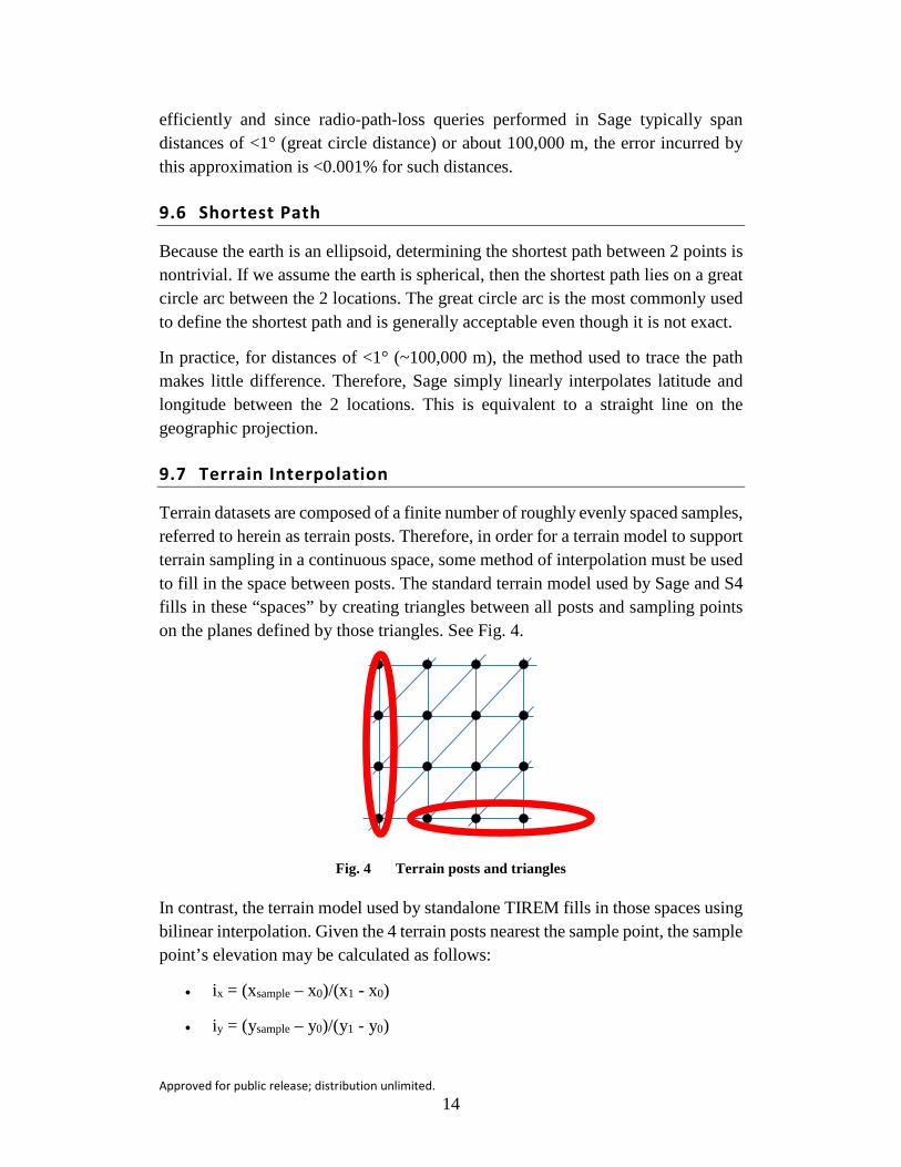
Terrain datasets are composed of a finite number of roughly evenly spaced samples, referred to herein as terrain posts. Therefore, in order for a terrain model to support terrain sampling in a continuous space, some method of interpolation must be used to fill in the space between posts. The standard terrain model used by Sage and S4 fills in these “spaces” by creating triangles between all posts and sampling points on the planes defined by those triangles. See Fig. 4.
Fig. 4 Terrain posts and triangles
In contrast, the terrain model used by standalone TIREM fills in those spaces using bilinear interpolation. Given the 4 terrain posts nearest the sample point, the sample point’s elevation may be calculated as follows:
• ix = (xsample – x0)/(x1 - x0)
• iy = (ysample – y0)/(y1 - y0)

Approved for public release; distribution unlimited. 15
• za = z00 * (1.0-ix) + z01 * ix
• zb = z10 * (1.0-ix) + z11 * ix
• zsample = za * (1.0-iy) + zb * iy
In the following calculations:
• ix and iy are interpolation factors.
• xsample and ysample, are the longitude and latitude of the location being sampled.
• x0, x1, y0, and y1, are the bounding longitudes and latitudes of the 4 nearest terrain posts to the sample.
• z00, z01, z10, and z11 are the elevation values of the 4 posts nearest to the sample.
• zsample is the resulting elevation of the sample point.
Columns share the same longitude and rows share the same latitude; refer back to Fig. 4.
10. Verification of Sage 2.0 Path Loss and SNR at the Simulation Level
Figure 5 shows a comparison of path-loss values computed in standalone TIREM and Sage TIREM. These data values typically match within 0.01 dB. These are the best-case comparisons because the terrain inputs for both models are exactly matched for these cases.
Fig. 5 Comparison of standalone TIREM to Sage TIREM for links with matching terrain profiles
Approved for public release; distribution unlimited. 16
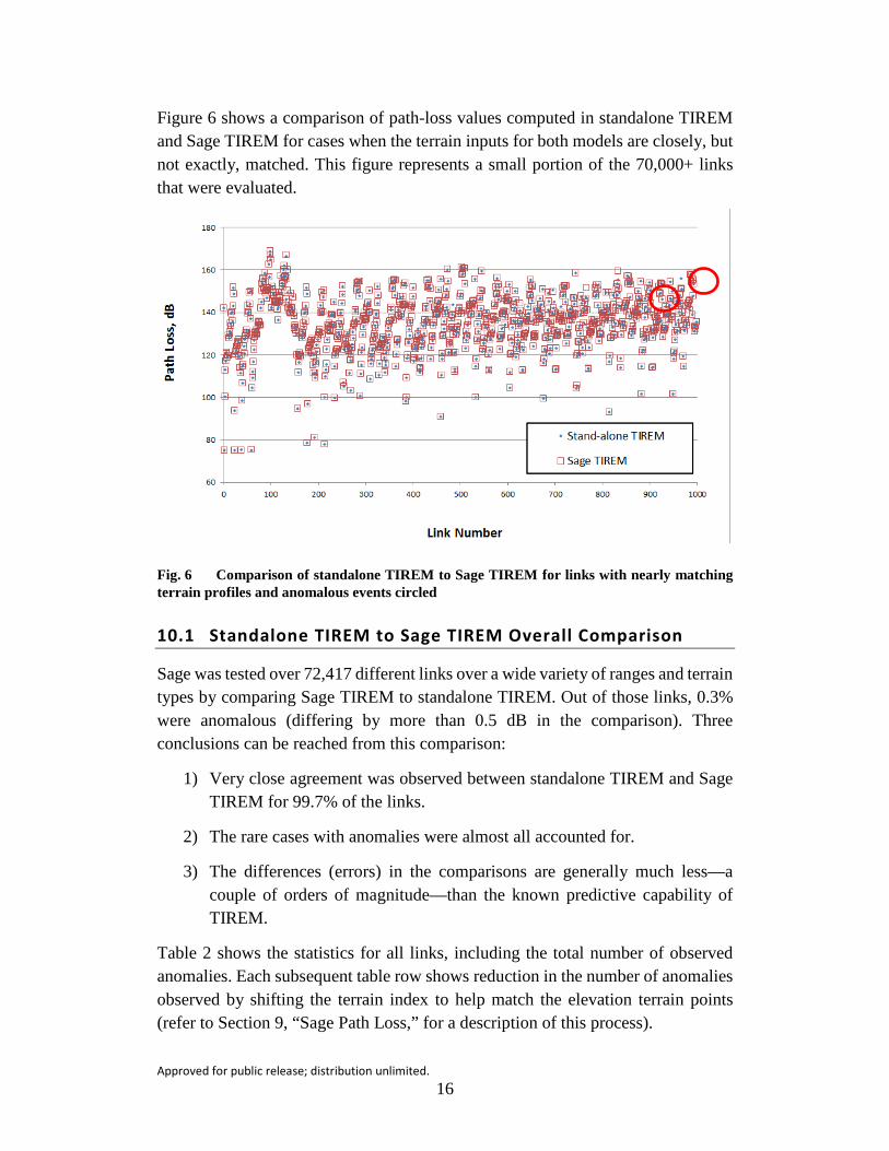
Figure 6 shows a comparison of path-loss values computed in standalone TIREM and Sage TIREM for cases when the terrain inputs for both models are closely, but not exactly, matched. This figure represents a small portion of the 70,000+ links that were evaluated.
Fig. 6 Comparison of standalone TIREM to Sage TIREM for links with nearly matching terrain profiles and anomalous events circled
10.1 Standalone TIREM to Sage TIREM Overall Comparison
Sage was tested over 72,417 different links over a wide variety of ranges and terrain types by comparing Sage TIREM to standalone TIREM. Out of those links, 0.3% were anomalous (differing by more than 0.5 dB in the comparison). Three conclusions can be reached from this comparison:
1) Very close agreement was observed between standalone TIREM and Sage TIREM for 99.7% of the links.
2) The rare cases with anomalies were almost all accounted for.
3) The differences (errors) in the comparisons are generally much less—a couple of orders of magnitude—than the known predictive capability of TIREM.
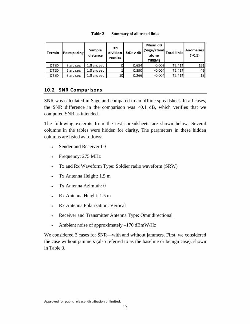
Table 2 shows the statistics for all links, including the total number of observed anomalies. Each subsequent table row shows reduction in the number of anomalies observed by shifting the terrain index to help match the elevation terrain points (refer to Section 9, “Sage Path Loss,” for a description of this process).
Approved for public release; distribution unlimited. 17
Table 2 Summary of all tested links
10.2 SNR Comparisons
SNR was calculated in Sage and compared to an offline spreadsheet. In all cases, the SNR difference in the comparison was <0.1 dB, which verifies that we computed SNR as intended.
The following excerpts from the test spreadsheets are shown below. Several columns in the tables were hidden for clarity. The parameters in these hidden columns are listed as follows:
• Sender and Receiver ID
• Frequency: 275 MHz
• Tx and Rx Waveform Type: Soldier radio waveform (SRW)
• Tx Antenna Height: 1.5 m
• Tx Antenna Azimuth: 0
• Rx Antenna Height: 1.5 m
• Rx Antenna Polarization: Vertical
• Receiver and Transmitter Antenna Type: Omnidirectional
• Ambient noise of approximately –170 dBmW/Hz
We considered 2 cases for SNR—with and without jammers. First, we considered the case without jammers (also referred to as the baseline or benign case), shown in Table 3.

Approved for public release; distribution unlimited. 18
Table 3 Spreadsheet for case with no jammer
More details of the step-wise verification between values obtained using standalone TIREM and Sage TIREM are shown in Table 4.
Table 4 Further details describing case with no jammer
Next, we considered the jammer case. As with the no jammer case, we assumed the following:
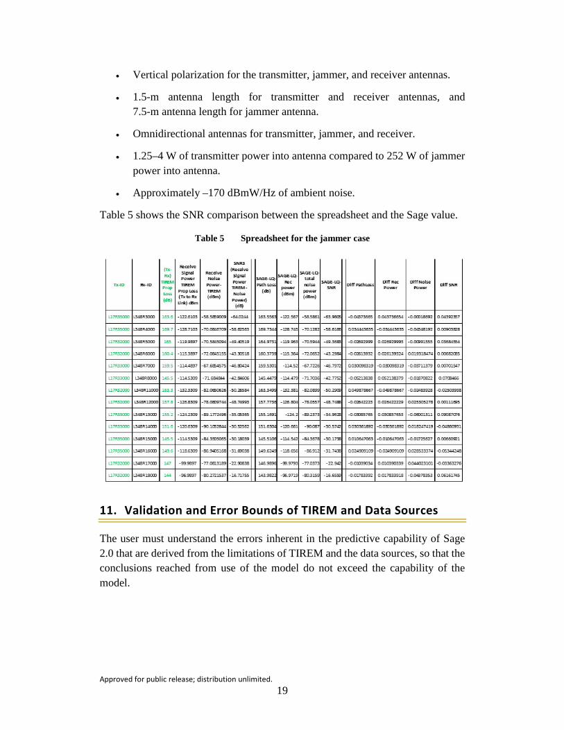
Approved for public release; distribution unlimited. 19
• Vertical polarization for the transmitter, jammer, and receiver antennas.
• 1.5-m antenna length for transmitter and receiver antennas, and 7.5-m antenna length for jammer antenna.
• Omnidirectional antennas for transmitter, jammer, and receiver.
• 1.25–4 W of transmitter power into antenna compared to 252 W of jammer power into antenna.
• Approximately –170 dBmW/Hz of ambient noise.
Table 5 shows the SNR comparison between the spreadsheet and the Sage value.
Table 5 Spreadsheet for the jammer case
11. Validation and Error Bounds of TIREM and Data Sources
The user must understand the errors inherent in the predictive capability of Sage 2.0 that are derived from the limitations of TIREM and the data sources, so that the conclusions reached from use of the model do not exceed the capability of the model.

Approved for public release; distribution unlimited. 20
11.1 TIREM V&V and Expected Accuracy
TIREM is a widely accepted and used industry standard in the US Army. Although there is not a single document summarizing TIREM V&V, there have been extensive measurements comparing TIREM predictions to real-world path loss.
The bottom line (gross approximation) is that the mean value of a large set of path losses is accurate within about 1.5 dB, with a standard deviation of about 10 dB. We accept the validity of TIREM within the fairly well-known error bounds. There is some ongoing debate about the use of TIREM accuracy with different resolution terrain data. Currently, DTED Level 1 terrain data for White Sands Missile Range, New Mexico’s Network Integration Evaluation test area is the accepted approach.
This has important implications for the SLAD analyst using Sage 2.0. Over a statistically significant set of data, the analyst can expect the mean value of the set of link quality predictions to be very accurate (1.5 dB in field conditions is difficult to measure accurately). On the other hand, the analyst should guard against making conclusions on individual links, as it is not uncommon for individual links to be in error by 10 dB (i.e., one standard deviation of error for TIREM), which is almost as much free space loss as would occur if the separation between radios were quadrupled.
11.2 Radio Data Sources
The following radio parameters are available in Sage 2.0, but generally should not be changed from default values, unless the user has great confidence in the rationale for making the change:
• Frequency
• Antenna height
• Antenna gain
• Antenna polarization
• Transmit power
• Receiver noise figure
Table 6 lists the sources for the values used for radio parameters.
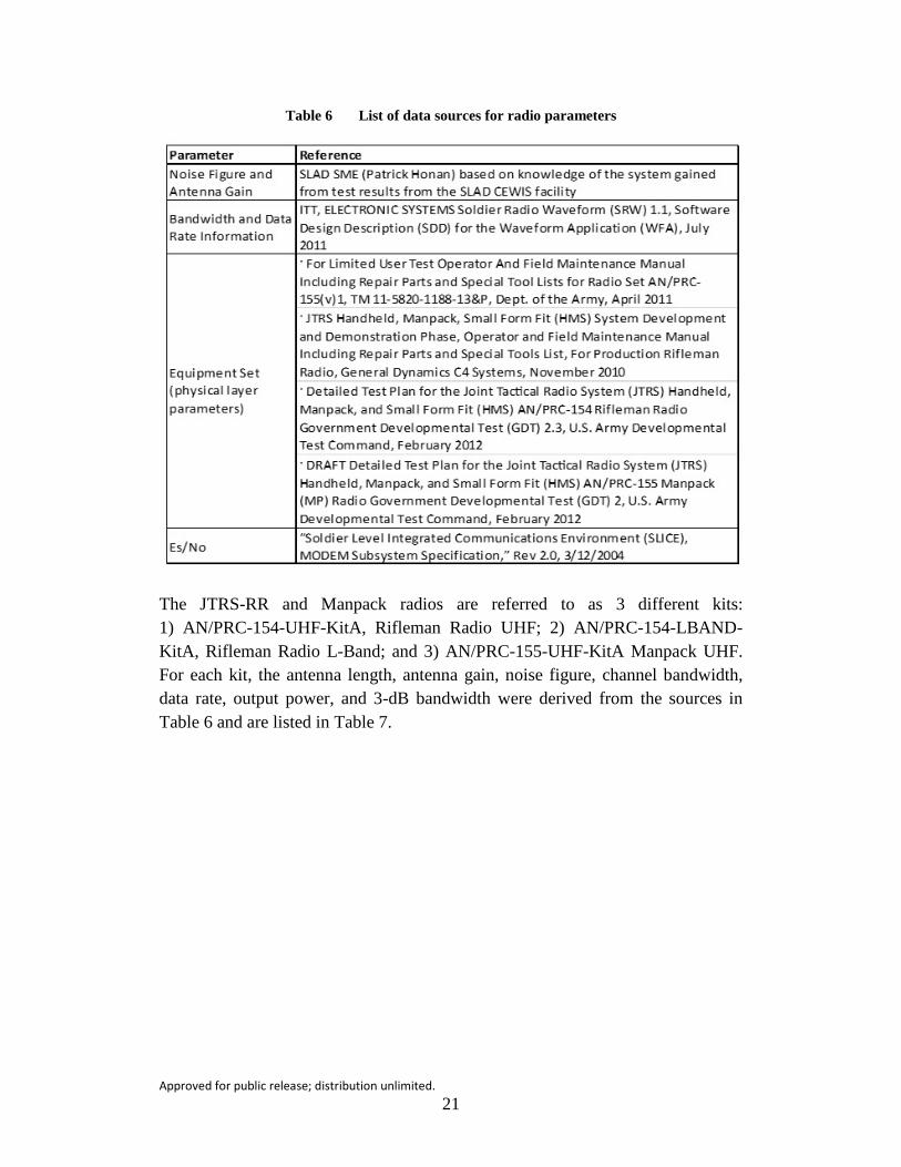
Approved for public release; distribution unlimited. 21
Table 6 List of data sources for radio parameters
The JTRS-RR and Manpack radios are referred to as 3 different kits: 1) AN/PRC-154-UHF-KitA, Rifleman Radio UHF; 2) AN/PRC-154-LBAND-KitA, Rifleman Radio L-Band; and 3) AN/PRC-155-UHF-KitA Manpack UHF. For each kit, the antenna length, antenna gain, noise figure, channel bandwidth, data rate, output power, and 3-dB bandwidth were derived from the sources in Table 6 and are listed in Table 7.
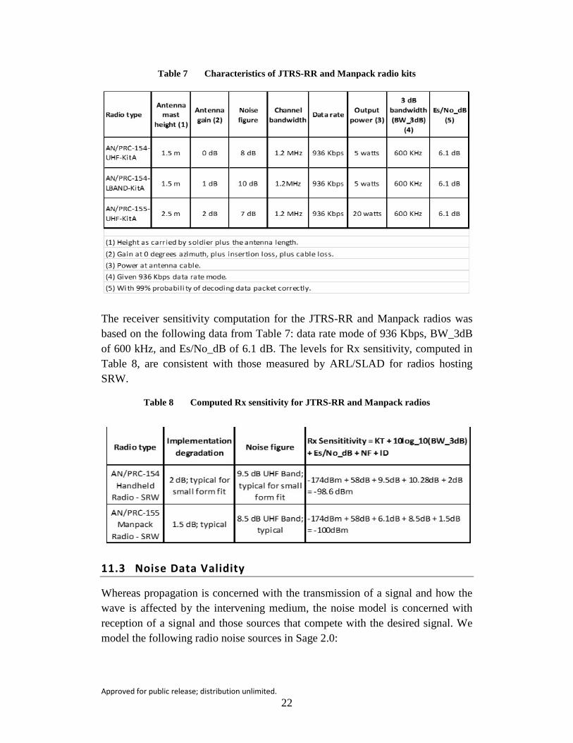
Approved for public release; distribution unlimited. 22
Table 7 Characteristics of JTRS-RR and Manpack radio kits
The receiver sensitivity computation for the JTRS-RR and Manpack radios was based on the following data from Table 7: data rate mode of 936 Kbps, BW_3dB of 600 kHz, and Es/No_dB of 6.1 dB. The levels for Rx sensitivity, computed in Table 8, are consistent with those measured by ARL/SLAD for radios hosting SRW.
Table 8 Computed Rx sensitivity for JTRS-RR and Manpack radios
11.3 Noise Data Validity
Whereas propagation is concerned with the transmission of a signal and how the wave is affected by the intervening medium, the noise model is concerned with reception of a signal and those sources that compete with the desired signal. We model the following radio noise sources in Sage 2.0:
Approved for public release; distribution unlimited. 23
• Ambient noise, consisting of a combination of galactic noise and man-made noise, modeled as data input to the simulation.
• Receiver noise (i.e., thermal noise and radio noise figure characteristics), modeled explicitly at an engineering level based on receiver characteristics such as frequency and channel bandwidth.
• Jammer noise, which undergoes path-loss modifications depending on jammer placement relative to radio receiver.
The ambient noise model has a large data component. The sources for noise data are referenced in the domain model specification.9 The validity of the noise model is largely attributed to the validity of the data sources.
Sage 2.0 uses noise data in a tabular format. This provides SLAD analysts the flexibility to implement different noise data depending on the environment being simulated. The V&V implication is that this data must come from an authoritative source.
The ambient noise table is set up with each row of the table having a frequency and corresponding noise power density (power/Hz). Sage 2.0 linearly interpolates between frequencies when data for a given frequency is not available in the table.
Ambient noise (in the baseline, nonjamming case) is assumed to be homogeneous in space and constant in time throughout the scenario. This provides several simplifying advantages, but it limits the ability to investigate situational awareness differences in regions of a scenario with nonhomogeneous noise characteristics.
Noise produced by a jammer is directional in nature because of Sage models directional jamming. Further, path loss between jammers and radios is modeled in TIREM and path loss varies with different intervening elevation profiles. Therefore, with a jammer present, noise is not homogeneous throughout the scenario.
Ambient noise, jammer noise, and internal receiver noise are combined through a simple summation. There are more accurate ways to combine noise sources, but this was considered sufficient by the domain experts, given the accuracy limitations of TIREM. Further, when jammer power dominates over other noise sources, the method used to combine noise sources tends to be less significant.

Approved for public release; distribution unlimited. 24
12. Conclusions
Sage 2.0 is verified and validated for link quality applications in rural terrain, subject to the intended use, constraints, limitations, and assumptions described in this report.
Approved for public release; distribution unlimited. 25
13. References
1. Bernstein R Jr, Flores R, Starks MW. Objectives and capabilities of the system of systems survivability simulation (S4). White Sands Missile Range (NM): Army Research Laboratory (US); 2006. Report No.: ARL-TN-260.
2. Military Operational Research Society. MORS Experimentation Lexicon; 2008. [accessed 2013 Apr] http://morsnet.pbworks.com/f/Experimentation +Lexicon+V1.1.doc.
3. Military Performance Specification. US Military specification digital terrain elevation data (DTED). Springfield (VA): National Imagery and Mapping Agency; 20 May 2000. MIL-PRF-89020B.
4. Austin KL, Bernstein R Jr. Verification and validation (V&V) methodology for the system of systems survivability simulation (S4). White Sands Missile Range (NM): Army Research Laboratory (US); 2011. Report No.: ARL-TR-5669.
5. Harikumar J, Honan P, Jackman J, Morgan B and Anderson L. Test data tables for “Verification and Validation of Rural Propagation in the Sage 2.0 Simulation”. Las Cruces (NM): NMSU Physical Science Laboratory (US); 2016. Report No.: PSL-REF-201606.
6. US Army RDECOM/CERDEC/Space and Terrestrial Communications Directorate/System Engineering Architecture Modeling and Simulation Division. Modeling and Simulation Verification and Validation Report for the Network Connectivity Analysis Model (NCAM), 30 Mar 2012.
7. Rice PL, Longley AG, Norton KA, and Barsis A. Transmission loss predictions for tropospheric communication circuits. Boulder (CO): Dept of Commerce (US); 1965. Report No.: NBS Technical Note 101.
8. Eppink D, Kuebler W. TIREM/SEM Handbook; ECAC-HDBK-93-076; Department of Defense Electromagnetic Compatibility Analysis Center: Annapolis, MD, 1994.
9. Harikumar J, Bothner P, Honan P. The noise domain model specification document – MR1; Las Cruces (NM): Physical Science Laboratory (US); 2012. Report No.: PSL-DMS-20120229.
Approved for public release; distribution unlimited. 26
List of Symbols, Abbreviations, and Acronyms
ARL US Army Research Laboratory
CLA constraint, limitation, and assumption
DMS domain model specifications
DTED US Military Specification Digital Terrain Elevation Data
ECAC Electromagnetic Compatibility Analysis Center
GPS Global Positioning System
JTRS-RR Joint Tactical Radio System-Rifleman Radio
NCAM Network Connectivity Analysis Model
NMSU New Mexico State University
PSL Physical Science Laboratory
RR rifleman radio
S4 System of Systems Survivability Simulation
SLAD Survivability/Lethality Analysis Directorate
SLV survivability, lethality, and vulnerability
SMS software model specifications
SNR signal-to-noise ratio
SRW Soldier radio waveform
TIREM Terrain Integrated Rough Earth Model
V&V verification and validation

Approved for public release; distribution unlimited. 27
1 DEFENSE TECHNICAL (PDF) INFORMATION CTR DTIC OCA 2 DIRECTOR (PDF) US ARMY RESEARCH LAB RDRL CIO L IMAL HRA MAIL & RECORDS MGMT 1 GOVT PRINTG OFC (PDF) A MALHOTRA 8 DIR US ARL (PDF) RDRL SLB R BOWEN RDRL SLE D BAYLOR R FLORES M STARKS L ANDERSON RDRL SLE M P SIMPSON RDRL SLE I JC ACOSTA D LANDIN 5 NEW MEXICO STATE UNIVERSITY (PDF) PHYSICAL SCIENCE LABORATORY R BERNSTEIN J HARIKUMAR P HONAN J JACKMAN B MORGAN

Approved for public release; distribution unlimited. 28
INTENTIONALLY LEFT BLANK.