on the validation of radio propagation modelsradio propagation models 2 j31. introduction ... rx...

On the Validation of Radio Propagation Models

Analytical validation of Network Simulator used

Propagation and Bit Error Rates Models

Hagen Paul [email protected]

ProtocolLabs

http://www.protocollabs.com

Munich, Germany

24. Januar 2010

mailto:[email protected]

Disclaimer

I The initial purpose of this work was to verify and check the implementation of the

Nakagami Fading Model in ns-3. At the half of the work I realized that the generated

material is a good starting point for path loss in general. Especially to develop

intuition how path loss influence the Wireless simulation at the whole. How model

knobs influences the characteristic of the channel, etc.

I The complete work is public available and can be used for further investigation:

git clone http://git.jauu.net/wireless-propagation.git

I Suggestion, enhancement or critic is highly welcome!

Radio Propagation Models 2 | 31

Introduction

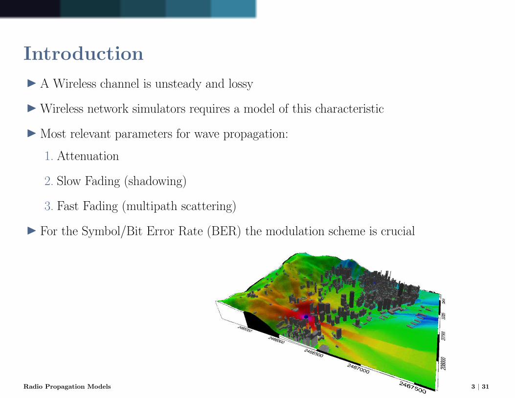
I A Wireless channel is unsteady and lossy

I Wireless network simulators requires a model of this characteristic

I Most relevant parameters for wave propagation:

1. Attenuation

2. Slow Fading (shadowing)

3. Fast Fading (multipath scattering)

I For the Symbol/Bit Error Rate (BER) the modulation scheme is crucial


Fresnel Zone

I The 1st Fresnel (pronounced Fray-nell) zone is a spheroid with its center along the

shortest distance between antennas.

I If there are no obstacles in the space forming 60% of this distance, propagation

characteristics are said to be the same as in free space

I Ensure line of sight between the transceivers

I If a Fresnel zone is not established, multipath interference will occur

I The Fresnelzone depends on the frequency: > F → < b

I Fn =√

nλd1d2d1+d2

, λ = vf


Attenuation

I So how to calculate the attenuation of a channel?

I How to map slow- and fast fading conditions?


Friis

I Friis is a transmission equation gives the power received by one antenna under

idealized conditions.

I Formula:

PrPt

= GtGr(λ

4πR)2

Pr Receiving power (dBm)

Pt Transmitter power (dBm)

Gt Antenna Gain Transmitter (dBi/dBd)

Gr Antenna Gain Receiver (dBi/dBd)

λ Wavelength (meter, . . . )

R Distance between the nodes (meter, . . . )

I But: ideal conditions are never achieved1

1one exception is satellite communications when there is negligible atmospheric absorptionRadio Propagation Models 6 | 31

-140

-120

-100

-80

-60

-40

-20

0

20

0 50 100 150 200 250 300 350 400 450 500

RX

Pow

er

[dbm

]

Node Distance [meter]

friis Path Loss Model

friis

Friis


Friis Wavelength Influences

-90

-80

-70

-60

-50

-40

-30

-20

-10

0 50 100 150 200 250 300 350 400 450 500

RX

Pow

er

[dbm

]


friis900 Path Loss Model

friis900

(a) Frequency: 900 Mhz (GSM)

-90

-80

-70

-60

-50

-40

-30

-20

-10

0 50 100 150 200 250 300 350 400 450 500

RX

Pow

er

[dbm

]


friis5000 Path Loss Model

friis5000

(b) Frequency: 5.0 GHz (802.11)

I The higher the frequency, the higher the loss.


Two Ray Ground

I Friis at long distance tends to accurate prediction

I The single line-of-sight path is seldom the only means of propagation

I The two-ray ground reflection model considers both the direct path and a ground

reflection path

I Pr(d) = PtGtGrh2th

2r

d4L

• L: 1

I Increased power loss compared to Free Space Model

I No good results for small distance→ use Free Space Model for near distances


-140

-120

-100

-80

-60

-40

-20

0

20

0 50 100 150 200 250 300 350 400 450 500

RX

Pow

er [

dbm

]


tworaygroundvanilla Path Loss Model

tworaygroundvanilla

Two Ray Ground (vanilla)


-140

-120

-100

-80

-60

-40

-20

0

20

0 50 100 150 200 250 300 350 400 450 500

RX

Pow

er [

dbm

]


tworayground Path Loss Model

tworayground

Two Ray Ground


-140

-120

-100

-80

-60

-40

-20

0

20

0 50 100 150 200 250 300 350 400 450 500

RX

Pow

er [

dbm

]


logdistance Path Loss Model

logdistance

Log Distance Model


-140

-120

-100

-80

-60

-40

-20

0

20

0 50 100 150 200 250 300 350 400 450 500

RX

Pow

er [

dbm

]


threelogdistance Path Loss Model

threelogdistance

Three Log Distance Model


Fading

I Fading is deviation of the attenuation

I Reasons:

• Shadowing from obstacles

•Multipath propagation

I Slow Fading

• Roughly constant amplitude and phase change over time

• Hills, buildings, . . .

• Often modeled using a log-normal distribution

I Fast fading

• Amplitude and phase change varies considerably

•Multiple reflections

I Modeled as a random process


-140

-120

-100

-80

-60

-40

-20

0

20

0 50 100 150 200 250 300 350 400 450 500

RX

Pow

er [

dbm

]


shadowing Path Loss Model

shadowing

Shadowing Model


-140

-120

-100

-80

-60

-40

-20

0

20

0 50 100 150 200 250 300 350 400 450 500

RX

Pow

er [

dbm

]


nakagami Path Loss Model

nakagami

Nakagami Model


-120

-100

-80

-60

-40

-20

0

20

0 50 100 150 200 250 300 350 400 450 500

RX

Pow

er [

dbm

]


Nakagami Dispersion Path Loss Model

Nakagami Dispersion

Nakagami Model Distribution


-100

-80

-60

-40

-20

0

0 50 100 150 200

RX

Pow

er [

dbm

]


Nakagami M0 Effects (d0m = 80) Path Loss Model

m0 = 0.25

m0 = 1.0

m0 = 1.5 (default)

m0 = 2.0

m0 = 5.0

Nakagami Model m0 Effect


-100

-80

-60

-40

-20

0

0 10 20 30 40 50 60 70 80

RX

Pow

er [

dbm

]


Nakagami M0 Effects (d0m = 80) Path Loss Model

m0 = 0.25

m0 = 1.0

m0 = 1.5 (default)

m0 = 2.0

m0 = 5.0

Nakagami Model m0 Effect


RX Power to SNR (1/2)

I Signal-to-Noise Ratio (SNR or S/N)

I Ratio of a signal power to the noise power corrupting the signal

I SNR =Psignal

Pnoise

I Noise:

• Boltzmann constant * Bandwidth * Receiver Noise * Implementation Loss

• Boltzmann constant (kB): 3.91−21 (B * Temp in Kelvin)

• Bandwidth: 206 Hz

• Receiver Noise: 15.8 W ( 12 dB)

• Implementation Loss: 1.58 W (2 dB)


RX Power to SNR (2/2)

I Noise: 1.99−12 Watt = −87dBm

I Example:

• Signal: -60 dBm

• Noise: -87 dBm

• SNR: -27 dB


Symbol/Bit Error Rate (1/3)

I Symbol Error Rate

I Common digital modulation schemes:

• Binary phase-shift keying (BPSK, 2 Symbols)

• Quadrature phase-shift keying (QPSK, 4 Symbols)

• 8 Phase-shift keying (8PSK, 8 Symbols)

• n-Quadrature amplitude modulation (QAM, 16, 32, 64 Symbols)

• . . .



I Symbol Error Rate vs. Es/No

I PS,MQAM = 2(1− 1√M

)erfc(√

32(M−1)

Es

E0)− (1− 2√

M+ 1

M )erfc2(√

32−(M−1)

Es

E0)

I Inverse Error Function (also known as Gauss error function):

• erfc(x) = 2√π

∫∞x e−t

2dt

I Symbol Error Rate→ Bit Error Rate:PS,MQAM

BitsperSymbol



1e-16

1e-14

1e-12

1e-10

1e-08

1e-06

0.0001

0.01

1

0 2 4 6 8 10 12 14 16

Sym

bol

Err

or

Rat

e [%

]

Es/No [dB]

Symbol error probability curve for various modulation schemes

BPSK

QAM4

4PAM

QAM16

16PSK


The End

I Questions?


SINR and IPW2200

I Signal-To-Noise Ratio (aka SNR and S/R)

I snr(dB) = signal level(dBm) - average noise level(dBm)

I Ratio of a signal power to the noise power corrupting the signal

I To receive a useful information the signal must clearly be higher then the noise

I Sidenote IPW2200 driver and /proc/net/wireless

• iwconfig eth1→ Link Quality=69/100 Signal level=-55 dBm Noise level=-82

dBm

• Noise: initial set to -85 dBm

• Every new packet updates the noise level (and average it with the previous one)

• priv->exp_avg_noise

• RSSI: received signal strength indication

• RSSI: a measurement of the power present in a received radio signal


• 0 to 255

• RSSI is acquired during the preamble stage of receiving an 802.11 frame

• RSSI is stored on the RX descriptor (stats.rssi) and is measured by baseband and

PHY for each individual packet

• see drivers/net/wireless/ipw2x00/ipw2200.c:ipw_rx()


Some Background on Antennas

I Basic types

• Omnidirectional

• Semi-directional

• Directional

I Omnidirectional

• Omnidirectional antennas radiate energy equally in all directions around the

antenna’s vertical axis

•Most common for WLAN: dipole antenna

I Semi-Directional

• Patch

• Panel

• Yagi

• Common examples: TV antennas or Cellular repeaters antennasRadio Propagation Models 28 | 31

I Highly Directional

• Parabolic dish

• Grid antenna


Common dbM/Watt Values2

I 80 dBm 100 kW Typical transmission power of FM radio station with 50 km range

I 60 dBm 1 kW = 1000 W Typical combined radiated RF power of microwave oven

elements

I 33 dBm 2 W Maximum output from a UMTS/3G mobile phone (Power class 1

mobiles)

I 30 dBm 1 W = 1000 mW Typical RF leakage from a microwave oven

I 20 dBm 100 mW Bluetooth Class 1 radio, 100 m range

I 15 dBm 32 mW Typical WiFi transmission power in laptops

I 4 dBm 2.5 mW Bluetooth Class 2 radio, 10 m range

I 0 dBm 1.0 mW = 1000 muW Bluetooth standard (Class 3) radio, 1 m range

I -10 dBm 100 muW Typical maximum received signal power (-10 to -30 dBm) of

wireless network2Source: WP


I -70 dBm 100 pW Typical range (-60 to -80 dBm) of wireless (802.11x) received signal

power over a network

I -127.5 dBm 0.178 fW = 178 aW Typical received signal power from a GPS satellite

I -174 dBm 0.004 aW = 4 zW Thermal noise floor for 1 Hz bandwidth at room

temperature (20 C)


on the validation of radio propagation modelsradio propagation models 2 j31. introduction ... rx...

Documents