VAT Notches, Voluntary Registration, and Bunching:

Theory and UK Evidence ∗

Li Liu and Ben Lockwood†

This version: July 2016

Abstract

We develop a conceptual framework that allows simultaneously for (i) voluntary

registration for VAT by firms below the registration threshold; and (ii) bunching at

the registration threshold. This framework also generates predictions about how vol-

untary registration and bunching are related to intensity of input use, the share of

B2C transactions for a firm, opportunities for evasion via under-reporting of sales, and

the competitiveness of the market in which the firm is located. We bring the theory

to the data, using linked administrative VAT and corporation tax records in the UK

from 2004-2009. Consistently with the theory, we find that voluntary registration is

positively related to the intensity of input use and negatively to the share of B2C

transactions, and the amount of bunching is related to these variables in the opposite

way. There is some evidence that product market competition leads to more voluntary

registration, and less bunching. In addition, we find some suggestive evidence that

firms are bunching by under-reporting sales.

∗This paper was previously circulated under the shorter title, “VAT Notches”. We thank the staff at HerMajesty’s Revenue & Customs’(HMRC) Datalab for access to the data and their support of this project.This work contains statistical data from HMRC which is Crown Copyright. The research datasets used maynot exactly reproduce HMRC aggregates. The use of HMRC statistical data in this work does not imply theendorsement of HMRC in relation to the interpretation or analysis of the information. All results have beenscreened by HMRC to ensure confidentiality is not breached.†Liu: Centre for Business Taxation, University of Oxford (li.liu@sbs.ox.ac.uk). Lockwood: CBT, CEPR

and Department of Economics, University of Warwick (b.lockwood@warwick.ac.uk). We would like to thankSteve Bond, Michael P. Devereux, Judith Freedman, Chris Heady, James R. Hines, Louis Kaplow, HenrikKleven, Tuomas Matikka, Joel Slemrod, and participants at the 2014 International Institute of Public FinanceMeeting, 2014 CEPR Public Economics Conference, Oxford-Michigan Tax Systems Conference, 2nd MaTaxConference in Mannheim, HM Treasury, Oxford University and University of Exeter for helpful comments.We would also like to thank Dongxian Guo and Omiros Kouvavas for excellent research assistance. Theusual disclaimer applies. We acknowledge financial support from the ESRC under grant ES/L000016/1.

1

1 Introduction

Most countries around the world use the value-added tax (VAT) as their primary indirect

tax, and most countries that adopted the VAT have thresholds, usually based on turnover,

below which businesses do not need to register for VAT.1 As VAT rates are often quite high

(in excess of 20% in many EU countries), this creates a large and salient tax notch for small

businesses whose turnover is around the threshold.2 So far, the effect of these VAT notches

on firm behavior has not received much attention.

In this paper, we make several contributions on this front, both theoretically, and em-

pirically, using administrative data on UK corporations. First, what are the stylized facts

to be explained? One striking feature of our data is that over the time period 2004-2009,

approximately 44% of firms with turnover below the threshold were registered for VAT. It

seems unlikely that this is entirely due to inertia - and indeed we present evidence below

to show that this is not the case - and so we conclude that some firms actively choose to

register, even if they are below the threshold. This is a striking phenomenon which deserves

further study; to our knowledge, voluntary payment of any tax is very rare.

Also, in our UK administrative data, there is strong evidence that some firms are re-

stricting their turnover to stay just below the registration threshold, i.e. they bunch. Apart

from intrinsic interest, these features are also important because they impact on production

ineffi ciencies induced by the VAT; when firms do not register, they face so-called embedded

VAT on inputs, which distorts input choices, and also cascades through the production chain

(Ebrill, Keen and Perry, 2001).

Our first contribution is to develop a simple general equilibrium model that can explain

both these phenomena in a unified way. Our first observation is that the coexistence of both

voluntary registration and bunching requires that firms make both sales to final consumers

(B2C sales) and sales to other VAT-registered businesses (B2B sales). To see this, suppose

first that firms make only B2C sales. Then, it is easily shown that irrespective of the degree

of competition between firms, the cost of voluntarily registering exceeds the benefit, because

the burden of VAT paid on output when registered exceeds the burden of VAT paid on inputs

when not registered. Conversely, with only B2B sales, the voluntary registration is always

optimal, because the burden of output VAT can be passed on to the buyer.3

Our second assumption is that firms have some market power, for reasons explained

1In the EU, all but two countries (Spain and Sweden) currently have positive thresholds, with the UKthreshold being the largest at £ 81,000. The thresholds in the EU are generally low compared with those incountries that have more recently introduced a VAT, such as Singapore, which currently has a threshold ofabout 540,000 Euro (http://www.vatlive.com).

2A notch arises when the tax liability changes discontinuously.3Both these points are made formally below.

2

in detail below. Finally, to study the effect of input costs on voluntary registration and

bunching, we must of course also assume that small firms use intermediate inputs as well

as labour in varying proportions. So, we construct the simplest general equilibrium model

that has the required features. The model can also be extended to allow for VAT evasion

via concealment of some fraction of B2C sales.

In this setting, we show the following. First, under some assumptions, the effect of the

VAT system on the registration decision can be captured by a VAT suffi cient statistic, which

combines the effects of both input and output VAT. We then show that voluntary registration

by a firm is more likely when either (i) the cost of inputs relative to sales is high, or (ii)

when the proportion of B2C sales by the firm is low.4 The intuition for (ii) is simply that if

most customers are VAT-registered, the burden of an increase in VAT can easily be passed

on in the form of a higher price, because the customer itself can claim back the increase.

The intuition for (i) is that when input costs are important, registration allows the firm to

claim back a considerable amount of input VAT.

Second, we show that the determinants of bunching at the registration threshold are

the same as for voluntary registration, with the signs of the effects reversed. Specifically,

bunching is more likely when (i) the cost of inputs relative to sales is low, or (ii) when the

proportion of B2C sales is high. Third, we study the effect of product market competition

on voluntary registration and bunching; the effects of increased competition are generally

ambiguous, but we identify the features that make it positive or negative.

Fourth, with evasion, the qualitative results obtained so far are unchanged. We show

that opportunities for evasion will increase voluntary registration and have an ambiguous

effect on bunching. The latter result is somewhat surprising, as it is usually assumed in the

empirical literature that bunching is facilitated by evasion opportunities. The explanation

here is that while concealment of sales does indeed make it easier for firms to stay below the

VAT threshold, at the same time, voluntary registration becomes more attractive, as output

VAT is less of a burden.

We then bring these predictions to an administrative data-set created by linking the

population of corporation and VAT tax records in the UK from 2004-2009. We first show

that the pattern of voluntary registration in the data is consistent with the theory. In

particular, voluntary registration is more likely with a low share of B2C sales or a high share

4Both these characteristics clearly differ widely across small firms that are close to the registrationthreshold. For example, a small tradesperson such as a plumber or electrician may typically have mostlyB2C sales of his services to householders, and make relatively light use of intermediate inputs. So, theywould face a low effective VAT rate when not registered, but a high rate when registered. Conversely, asmall specialist engineering firm, such as a car component firm, may make mostly B2B sales with heavy useof intermediate inputs, and so will be in the reverse position.

3

of input costs. Quantitatively, the probability that a firm voluntarily registers for VAT is

increased by 5 percentage points for a one standard deviation increase in the share of B2C

sales and by 2-5 percentage points for a one standard deviation increase in the input cost

ratio. The results are robust to use of either a linear probability model or fixed-effects logit

model, and to the inclusion of additional firm-level control variables.

We then look at bunching. In the aggregate, there is clear evidence of bunching at

the VAT threshold. Investigating further, we find that firms are more likely to bunch at

the threshold when either (i) the cost of inputs relative to sales is high, or (ii) when the

proportion of B2C sales is low, consistently with the theory. So, there is a clear pattern of

heterogeneity in bunching.

We also investigate the mechanisms at work in bunching. We provide some suggestive

evidence that part of bunching is driven by evasion, in the form of under-reporting of sales.

Specifically, we find that the average input cost ratio moves in parallel between the registered

and non-registered firms outside the bunching region but starts to increase substantially for

the non-registered companies just below the threshold.

Finally, in the last section, we study the dynamic movement of firms in and out of

registration status. Specifically, we address the concern that voluntary registration may

not be an optimizing choice of firms, but simply a failure to deregister, once having been

above the threshold and having registered. Our empirical findings suggest that while there

is a considerable amount of persistence in firm behavior, the decision is not entirely driven

by inertia; firms change their registration decisions in a way that is consistent with profit

maximizing behavior.

The rest of the paper proceeds as follows. The next section reviews related literature.

Section 3 develops the conceptual framework to analyze VAT bunching and voluntary regis-

tration. Section 4 derives the main empirical predictions. Section 5 provides an overview of

the VAT system in the UK and describes the data. Sections 6 and 7 present the empirical

analysis for voluntary registration and VAT bunching, respectively. Section 8 studies the

dynamic movement of firms in and out of registration status. Finally, Section 9 concludes.

2 Related Literature

Our work contributes to several strands of literature, other than those already discussed.

First, our work relates to the literature on the effect of tax and regulatory thresholds, and in

particular, the effect of VAT thresholds on small business behavior. In an important paper,

Keen and Mintz (2004) were the first to set up a model of VAT including a threshold; they

show that there will be bunching below the threshold, and a “hole”above, where firms do

4

not locate. However, there are a number of differences between their approach and ours.5

First, their model has only final consumers (i.e. only B2C sales), and so, as argued above,

cannot explain voluntary registration. Second, their main focus is on the optimal registration

threshold, whereas ours is on the coexistence and determinants of voluntary registration and

bunching. Kanbur and Keen (2014) extend the Keen and Mintz (2004) framework to allow

for evasion, as well as avoidance, of VAT. Brashares et al. (2014) use a calibrated formula

from Keen and Mintz (2004) to infer that for a 10 percent VAT rate, the optimal level for

the threshold in the United States is $200,000.6

There is a small empirical literature on the effects of VAT thresholds. Onji (2009) doc-

uments the effects of the VAT threshold in Japan, focusing on the incentives for a large

firm to split by separately incorporating. A comparison of the corporate size distributions

before and after the VAT introduction of 1989 shows a clustering of corporations just below

the threshold. Recent papers following our work document bunching of small firms at the

VAT registration threshold in Finland (Harju, Matikka and Rauhanen (2016)) as well as

lack of bunching in response to the VAT threshold in Armenia (Asatryan and Peichl (2016)).

In particular, Harju, Matikka and Rauhanen (2016) provide strong evidence for Finland

that bunching below the threshold occurs, and that compliance costs can explain a major

part of bunching. However, neither of these papers studies the determinants of voluntary

registration in detail, nor do they develop a theoretical framework specific to the VAT.7

There are several reasons that compliance costs may be more important in Finland than

for our study. First, the VAT threshold in Finland is very low, at 8,500 Euro, compared

to well over 100,000 Euro in the UK over our period. Other things equal, larger firms find

compliance less costly. Second, in the UK, all active companies are required to file company

accounts and corporation tax returns, so they already have the information required for the

VAT return, and the VAT return itself is short and simple. Finally, a simplified VAT scheme,

5The main focus of their paper is to study the optimal VAT threshold, a topic beyond the scope of thispaper.

6There is also a literature on VAT and the choice of informality in developing countries (Emran andStiglitz (2005), de Paula and Scheinkman (2010)). In particular, de Paula and Scheinkman (2010) present amodel where firms can choose between formal production, where they must register for VAT, and informalproduction; they can also choose between buying inputs from a formal and informal supplier. The focus ofthe paper is on the informality choice with an application to Brazil.

7Harju, Matikka and Rauhanen (2016) present formulae for the reduced form elasticity implied by observedbunching which are taken directly from Kleven and Waseem (2013). However, these formulae are originallydeveloped for a labour supply model, and care must be shown when applying them to VAT. In particular, inan earlier version of this paper Liu and Lockwood (2015), we show that to apply the Kleven-Waseem formulaedirectly, it must be assumed that all sales are B2C, firms are price-takers, and the production function isfixed-coeffi cients must be assumed. Moreover, the elasticity estimated is an output supply elasticity, takingthe price of output as given, not the elasticity of the tax base, because the latter will also be determined bythe elasticity of demand.

5

the Flat-Rate Scheme (FRS), was introduced in the UK in 2002 to reduce compliance costs

for small businesses; however, the FRS had a low take-up rate of around 3% among all

eligible VAT traders, and there is no bunching at the FRS threshold above which firms are

no longer eligible for FRS, suggesting that firms do not try to bunch to avoid the additional

compliance costs of normal VAT registration (Vesal, 2013).8

More broadly, there are a few papers on the effects of other kinds of thresholds. The

most relevant is Almunia and Lopez Rodriguez (2014), who study a threshold in Spain

where firms with turnover above 6 million Euro face increased tax enforcement. Almunia

and Lopez Rodriguez (2014) show that firms bunch at this threshold, and that bunching is

more pronounced, the lower the fraction of B2C sales in the total for the sector. This is of

course, the reverse to what we find. Their explanation is that if sales are mostly to other

firms, if audited, a firm will have a “paper trail”that will make it relatively easy to cross-

check tax returns to detect misreported intermediate input sales. The contrast between the

results of Almunia and Lopez Rodriguez (2014) and ours indicates that the purpose of the

turnover threshold is crucial i.e. whether it relates to a change in tax liability - as in our

case- or enforcement of a given tax liability, as in theirs.9

Our work also relates to the literature on tax notches (Slemrod (2010), Kleven and

Waseem (2013), Best and Kleven (2013), Kopczuk and Munroe (2015), and Kleven (2016)).

In particular, Kleven and Waseem (2013) emphasize that if individuals behave fully ration-

ally, notches give rise to bunching below the threshold, and “holes”above the threshold where

maximizing agents will not locate, and then uses bunching to estimate both the elasticity

of labour supply, and the degree of optimization frictions. As shown below, the “bunching

equation” in this paper, which relates the amount of bunching to the elasticity of the tax

base and parameters of the tax system, is mathematically very similar to the equation of

(Kleven and Waseem (2013)). However, for reasons discussed below, it is much more diffi cult

to back out credible elasticity estimates in the VAT case, and so we do not attempt this in

the paper.

Also, because we study evasion, our paper further relates to recent literature using special

features of tax systems to identify evasion from kinks and notches. For example, Best et al.

(2015) study a minimum tax scheme for corporations in Pakistan which has a kink point

where the real incentive for bunching is small, but the evasion incentive is large, and they

8Consistently with this, direct evidence on compliance costs for the UK put costs at around 1.5% ofturnover for firms around the registration threshold (Federation of Small Businesses, 2010), which is relativelysmall compared to the burden of VAT at 20%.

9It may be possible that being registered for VAT increases the probability of audit. Howoever, in ourdata, this effect may be attenuated by the fact that all firms, VAT-registered or not, are also companies andthus file a corporate tax return.

6

find large bunching around the minimum tax kink.10 However, we do not measure evasion

directly, nor, given the UK VAT system, do we have any obvious way of decomposing the

total bunching effect into bunching due to evasion, and that due to a real response. Rather,

we show that our theoretical predictions are robust to evasion.

3 Conceptual Framework

Key Features of the Model. As described in the introduction, we aim to model the

behavior of “small” firms selling to both final consumers and to businesses, where both

voluntary registration and bunching can be equilibrium outcomes. The first point is that the

coexistence of both voluntary registration and bunching requires that the “small”firms make

both B2B and B2C sales. To see this, suppose first that firms make only B2C sales. Then,

it is easily shown that irrespective of the degree of competition between firms, the cost of

voluntarily registering exceeds the benefit, because the burden of VAT paid on output when

registered exceeds the burden of VAT paid on inputs when not registered. Conversely, with

only B2B sales, the voluntary registration is always optimal, because the burden of output

VAT can be passed on to the buyer.11

Second, in order to study the effect of the input cost ratio transactions on voluntary regis-

tration and bunching, we must of course also assume that the “small”firms use intermediate

inputs as well as labour in varying proportions, so this must be a feature of the model.

A final assumption is that the small firms have some market power; this is for two reasons.

First, because as explained in the not-for-publication appendix in Section B, the simplest

perfectly competitive model which allows for both B2B and B2C sales has some undesirable

features; specifically, there is complete sorting,12 which is not observed in practice, and the

structure of the equilibrium is more complex than with monopolistic competition. Second,

in practice, markets are not perfectly competitive, and it is interesting to ask what the effect

of the degree of competition are on voluntary registration and bunching.

So, we construct the simplest general equilibrium model that has the required features.

There is a single representative consumer that supplies labour and buys two kinds of goods; a

differentiated good sold by the small firms, and a single good produced by a large firm. The

large firm also buys inputs from the small firms, generating a B2B demand. We assume that

the large firm is operating at a scale where non-registration for VAT (i.e. operating so that

10More recently, Waseem (2016), again for Pakistan, shows very large responses when reforms cut the rateof income tax to zero for the self-employed, which he interprets as being largely an evasion response.11Both these points are made formally below in the context of our model, and are shown formally in the

not-for-publication appendix.12That is, registered firms sell only B2B, and non-registered firms sell only B2C.

7

the value of sales are below the VAT threshold) is never profitable. Finally, a homogenous

input to the small firm is produced by a third sector of competitive firms from a labour

input via a constant returns technology. The behavior of this last sector is summarized by

a zero-profit condition that says that the price of the small-firm input is equal to the wage.

The structure of this economy is illustrated in Figure 1.

Consumers. There is a representative household that has preferences over the homogen-ous good, consumed at level Y, a set of differentiated goods a ∈ [a, a], consumed at levels

x(a), a ∈ [a, a], and leisure l. These preferences are of the following form:

U(X) + V (Y ) + l, X =

[∫ a

a

(x(a))(eC−1)/eC da

]eC/(eC−1)

, eC > 1 (1)

where X is a CES index of differentiated products, and

U(X) = λ1/φ X1−1/φ

1− 1/φ, V (Y ) = (1− λ)1/γ Y

1−1/γ

1− 1/γ, φ > 0, γ > 1

Each differentiated good a is produced by a single small firm a, which can be either registered

for VAT or not. For reasons further discussed below, we also allow the homogenous good Y

to be subject to VAT or not. So, the household faces a budget constraint

P (1 + J.t)Y +

∫ a

a

(p(a)(1 + I(a)t) (x(a))(eC−1)/eC da = w(1− l) (2)

where and 1 − l is labour supply, w is the wage, P is the price of the homogenous good

produced by the large firm, p(a) is the price excluding VAT of the small firm a′s output,

and where I(a) ∈ {0, 1} is an indicator recording whether the firm registers for VAT or not,

with a “1”indicating registration. So, if the firm is registered, the consumer price is grossed

up by VAT i.e. p(a)(1 + t). Finally, J ∈ {0, 1} records whether Y is subject to output VAT.

Our baseline case is J = 1, but J = 0 allows an interpretation of the model as a small open

economy where Y is exported; see Section 3.1 below. Consistently with this interpretation,

we assume that if J = 0, good Y is zero-rated for VAT, rather than exempt, so that the

large firm can still claim back input VAT.13

So, by standard arguments, maximization of (1) subject to (2) gives household demand

13If the large firm were exempt, there would be no difference, from a VAT point of view, between B2Band B2C demand.

8

for the homogenous and differentiated goods:

Y = (1− λ)(1 + J.t)−γP−γ (3)

x(a) = λ

((p(a)(1 + I(a)t))

Q

)−eCQ−φ (4)

where Q is the CES price index corresponding to the quantity index X.14 We assume that

in equilibrium, positive leisure is consumed, so that from (1), the wage is fixed at unity.

The Large Firm. The large firm combines inputs y(a), a ∈ [a, a] bought from the small

firms via a constant returns CES production technology to produce output Y. This production

technology is characterized by a CES cost function per unit of output of

C =

[∫ a

a

(p(a))1−eB da

]1/(1−eB)

, eB > 1

where p(a) is the price of the input net of tax (as the large firm is VAT-registered, it can claim

back any tax on inputs). So, the large firm chooses p to maximize (1− λ)P−γ(P −C). This

gives the usual mark-up equation for price i.e.

P =γ

γ − 1C (5)

and thus, combining (5),(3), ultimately, output is

Y = (1− λ)(1 + J.t)−γ(

γ

γ − 1C

)−γ(6)

Finally, input demand for variety a is, by Shepard’s Lemma and (6):

y(a) =∂C

∂p(a)Y = (1− λ)(1 + J.t)−γ

(γ

γ − 1

)−γC−γ

(p(a)

C

)−eB(7)

The Small Firms. A small firm’s technology is assumed constant returns and CES, likethe large firm, it is described by the unit cost function, which is specified as:

c(I(a); a) =1

a

(ωr(1 + I(a)t)1−σ + (1− ω)w

)1/(1−σ)(8)

14That is,

Q =

[∫ a

a

((1 + I(a)t)p(a))1−eCda

]1/(1−eC)

9

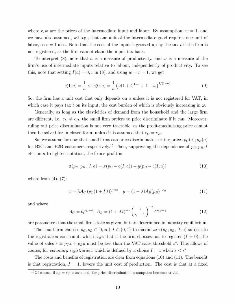
where r, w are the prices of the intermediate input and labor. By assumption, w = 1, and

we have also assumed, w.l.o.g., that one unit of the intermediate good requires one unit of

labor, so r = 1 also. Note that the cost of the input is grossed up by the tax t if the firm is

not registered, as the firm cannot claim the input tax back.

To interpret (8), note that a is a measure of productivity, and ω is a measure of the

firm’s use of intermediate inputs relative to labour, independently of productivity. To see

this, note that setting I(a) = 0, 1 in (8), and using w = r = 1, we get

c(1; a) =1

a< c(0; a) =

1

a

(ω(1 + t)1−σ + 1− ω

)1/(1−σ)(9)

So, the firm has a unit cost that only depends on a unless it is not registered for VAT, in

which case it pays tax t on its input, the cost burden of which is obviously increasing in ω.

Generally, as long as the elasticities of demand from the household and the large firm

are different, i.e. eC 6= eB, the small firm prefers to price discriminate if it can. Moreover,

ruling out price discrimination is not very tractable, as the profit-maximising price cannot

then be solved for in closed form, unless it is assumed that eC = eB.

So, we assume for now that small firms can price-discriminate, setting prices pC(a), pB(a)

for B2C and B2B customers respectively.15 Then, suppressing the dependence of pC , pB, I

etc. on a to lighten notation, the firm’s profit is

π(pC , pB, I; a) = x(pC − c(I; a)) + y(pB − c(I; a)) (10)

where from (4), (7):

x = λAC (pC(1 + I.t))−eC , y = (1− λ)AB(pB)−eB (11)

and where

AC = QeC−φ, AB = (1 + J.t)−γ(

γ

γ − 1

)−γCeB−γ (12)

are parameters that the small firms take as given, but are determined in industry equilibrium.

The small firm chooses pC , pB ∈ [0,∞), I ∈ {0, 1} to maximize π(pC , pB, I; a) subject to

the registration constraint, which says that if the firm chooses not to register (I = 0), the

value of sales s ≡ pCx + pBy must be less than the VAT sales threshold s∗. This allows of

course, for voluntary registration, which is defined by a choice I = 1 when s < s∗.

The costs and benefits of registration are clear from equations (10) and (11). The benefit

is that registration, I = 1, lowers the unit cost of production. The cost is that at a fixed

15Of course, if eB = eC is assumed, the price-discrimination assumption becomes trivial.

10

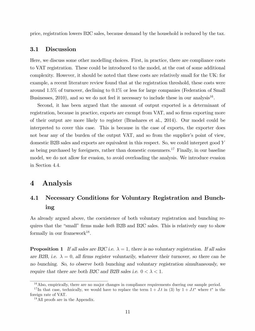
price, registration lowers B2C sales, because demand by the household is reduced by the tax.

3.1 Discussion

Here, we discuss some other modelling choices. First, in practice, there are compliance costs

to VAT registration. These could be introduced to the model, at the cost of some additional

complexity. However, it should be noted that these costs are relatively small for the UK: for

example, a recent literature review found that at the registration threshold, these costs were

around 1.5% of turnover, declining to 0.1% or less for large companies (Federation of Small

Businesses, 2010), and so we do not feel it necessary to include these in our analysis16.

Second, it has been argued that the amount of output exported is a determinant of

registration, because in practice, exports are exempt from VAT, and so firms exporting more

of their output are more likely to register (Brashares et al., 2014). Our model could be

interpreted to cover this case. This is because in the case of exports, the exporter does

not bear any of the burden of the output VAT, and so from the supplier’s point of view,

domestic B2B sales and exports are equivalent in this respect. So, we could interpret good Y

as being purchased by foreigners, rather than domestic consumers.17 Finally, in our baseline

model, we do not allow for evasion, to avoid overloading the analysis. We introduce evasion

in Section 4.4.

4 Analysis

4.1 Necessary Conditions for Voluntary Registration and Bunch-

ing

As already argued above, the coexistence of both voluntary registration and bunching re-

quires that the “small”firms make both B2B and B2C sales. This is relatively easy to show

formally in our framework18.

Proposition 1 If all sales are B2C i.e. λ = 1, there is no voluntary registration. If all sales

are B2B, i.e. λ = 0, all firms register voluntarily, whatever their turnover, so there can be

no bunching. So, to observe both bunching and voluntary registration simultaneously, we

require that there are both B2C and B2B sales i.e. 0 < λ < 1.

16Also, empirically, there are no major changes in compliance requirements duering our sample period.17In that case, technically, we would have to replace the term 1 + J.t in (3) by 1 + J.t∗ where t∗ is the

foreign rate of VAT.18All proofs are in the Appendix.

11

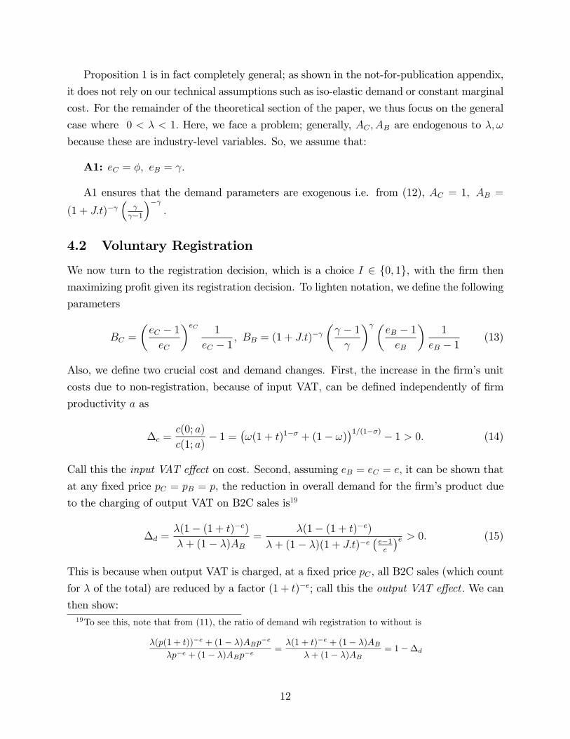
Proposition 1 is in fact completely general; as shown in the not-for-publication appendix,

it does not rely on our technical assumptions such as iso-elastic demand or constant marginal

cost. For the remainder of the theoretical section of the paper, we thus focus on the general

case where 0 < λ < 1. Here, we face a problem; generally, AC , AB are endogenous to λ, ω

because these are industry-level variables. So, we assume that:

A1: eC = φ, eB = γ.

A1 ensures that the demand parameters are exogenous i.e. from (12), AC = 1, AB =

(1 + J.t)−γ(

γγ−1

)−γ.

4.2 Voluntary Registration

We now turn to the registration decision, which is a choice I ∈ {0, 1}, with the firm then

maximizing profit given its registration decision. To lighten notation, we define the following

parameters

BC =

(eC − 1

eC

)eC 1

eC − 1, BB = (1 + J.t)−γ

(γ − 1

γ

)γ (eB − 1

eB

)1

eB − 1(13)

Also, we define two crucial cost and demand changes. First, the increase in the firm’s unit

costs due to non-registration, because of input VAT, can be defined independently of firm

productivity a as

∆c =c(0; a)

c(1; a)− 1 =

(ω(1 + t)1−σ + (1− ω)

)1/(1−σ) − 1 > 0. (14)

Call this the input VAT effect on cost. Second, assuming eB = eC = e, it can be shown that

at any fixed price pC = pB = p, the reduction in overall demand for the firm’s product due

to the charging of output VAT on B2C sales is19

∆d =λ(1− (1 + t)−e)

λ+ (1− λ)AB=

λ(1− (1 + t)−e)

λ+ (1− λ)(1 + J.t)−e(e−1e

)e > 0. (15)

This is because when output VAT is charged, at a fixed price pC , all B2C sales (which count

for λ of the total) are reduced by a factor (1 + t)−e; call this the output VAT effect . We can

then show:19To see this, note that from (11), the ratio of demand wih registration to without is

λ(p(1 + t))−e + (1− λ)ABp−e

λp−e + (1− λ)ABp−e=λ(1 + t)−e + (1− λ)AB

λ+ (1− λ)AB= 1−∆d

12

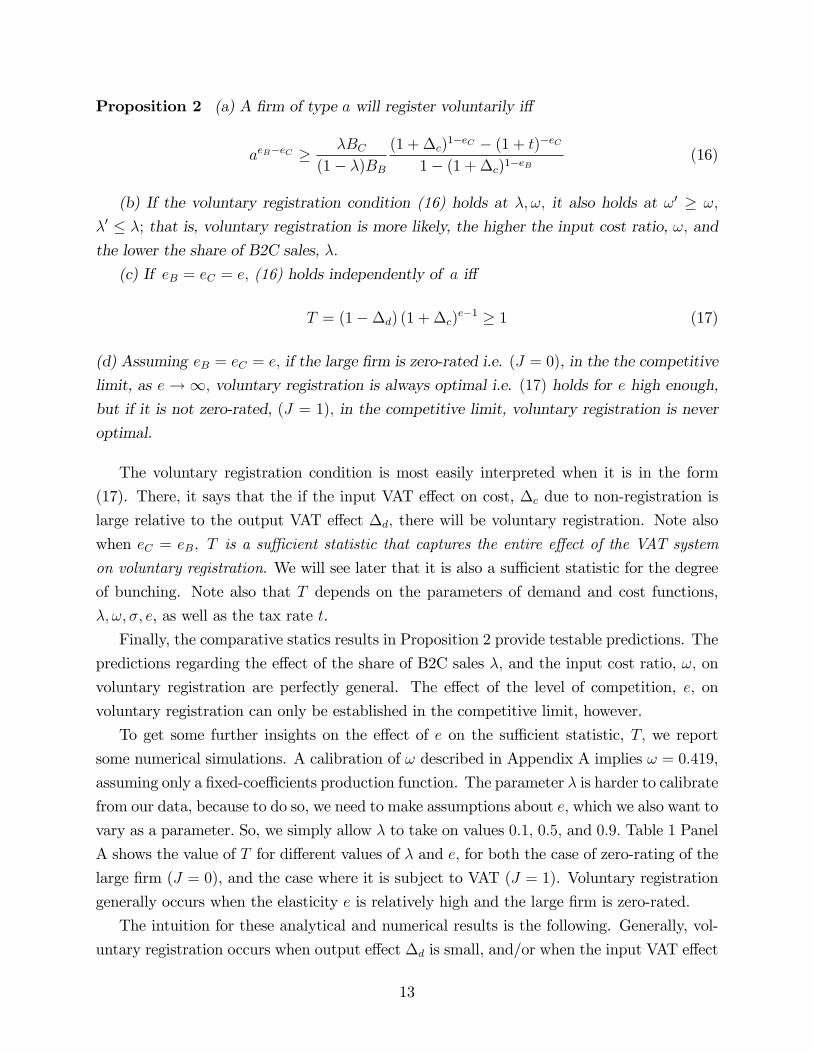
Proposition 2 (a) A firm of type a will register voluntarily iff

aeB−eC ≥ λBC

(1− λ)BB

(1 + ∆c)1−eC − (1 + t)−eC

1− (1 + ∆c)1−eB(16)

(b) If the voluntary registration condition (16) holds at λ, ω, it also holds at ω′ ≥ ω,

λ′ ≤ λ; that is, voluntary registration is more likely, the higher the input cost ratio, ω, and

the lower the share of B2C sales, λ.

(c) If eB = eC = e, (16) holds independently of a iff

T = (1−∆d) (1 + ∆c)e−1 ≥ 1 (17)

(d) Assuming eB = eC = e, if the large firm is zero-rated i.e. (J = 0), in the the competitive

limit, as e→∞, voluntary registration is always optimal i.e. (17) holds for e high enough,

but if it is not zero-rated, (J = 1), in the competitive limit, voluntary registration is never

optimal.

The voluntary registration condition is most easily interpreted when it is in the form

(17). There, it says that the if the input VAT effect on cost, ∆c due to non-registration is

large relative to the output VAT effect ∆d, there will be voluntary registration. Note also

when eC = eB, T is a suffi cient statistic that captures the entire effect of the VAT system

on voluntary registration. We will see later that it is also a suffi cient statistic for the degree

of bunching. Note also that T depends on the parameters of demand and cost functions,

λ, ω, σ, e, as well as the tax rate t.

Finally, the comparative statics results in Proposition 2 provide testable predictions. The

predictions regarding the effect of the share of B2C sales λ, and the input cost ratio, ω, on

voluntary registration are perfectly general. The effect of the level of competition, e, on

voluntary registration can only be established in the competitive limit, however.

To get some further insights on the effect of e on the suffi cient statistic, T, we report

some numerical simulations. A calibration of ω described in Appendix A implies ω = 0.419,

assuming only a fixed-coeffi cients production function. The parameter λ is harder to calibrate

from our data, because to do so, we need to make assumptions about e, which we also want to

vary as a parameter. So, we simply allow λ to take on values 0.1, 0.5, and 0.9. Table 1 Panel

A shows the value of T for different values of λ and e, for both the case of zero-rating of the

large firm (J = 0), and the case where it is subject to VAT (J = 1). Voluntary registration

generally occurs when the elasticity e is relatively high and the large firm is zero-rated.

The intuition for these analytical and numerical results is the following. Generally, vol-

untary registration occurs when output effect ∆d is small, and/or when the input VAT effect

13

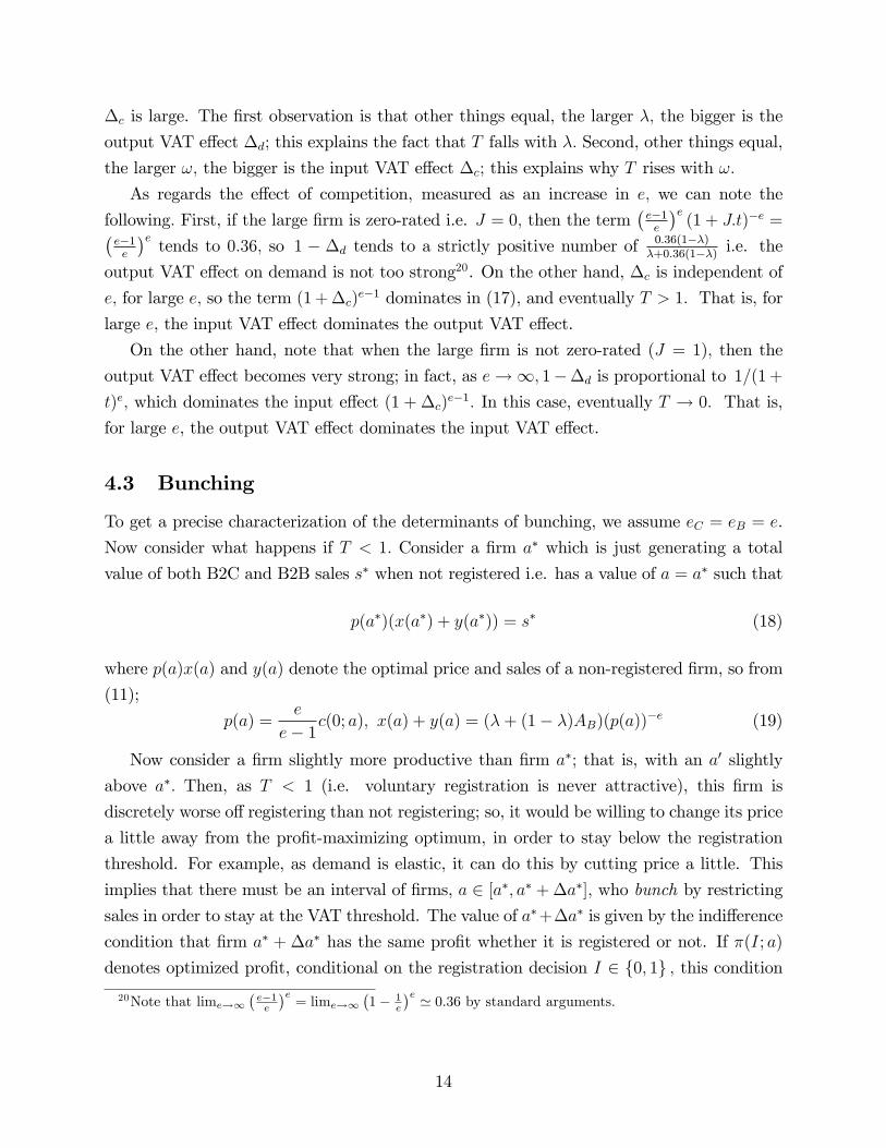
∆c is large. The first observation is that other things equal, the larger λ, the bigger is the

output VAT effect ∆d; this explains the fact that T falls with λ. Second, other things equal,

the larger ω, the bigger is the input VAT effect ∆c; this explains why T rises with ω.

As regards the effect of competition, measured as an increase in e, we can note the

following. First, if the large firm is zero-rated i.e. J = 0, then the term(e−1e

)e(1 + J.t)−e =(

e−1e

)etends to 0.36, so 1 − ∆d tends to a strictly positive number of

0.36(1−λ)λ+0.36(1−λ)

i.e. the

output VAT effect on demand is not too strong20. On the other hand, ∆c is independent of

e, for large e, so the term (1 + ∆c)e−1 dominates in (17), and eventually T > 1. That is, for

large e, the input VAT effect dominates the output VAT effect.

On the other hand, note that when the large firm is not zero-rated (J = 1), then the

output VAT effect becomes very strong; in fact, as e→∞, 1−∆d is proportional to 1/(1 +

t)e, which dominates the input effect (1 + ∆c)e−1. In this case, eventually T → 0. That is,

for large e, the output VAT effect dominates the input VAT effect.

4.3 Bunching

To get a precise characterization of the determinants of bunching, we assume eC = eB = e.

Now consider what happens if T < 1. Consider a firm a∗ which is just generating a total

value of both B2C and B2B sales s∗ when not registered i.e. has a value of a = a∗ such that

p(a∗)(x(a∗) + y(a∗)) = s∗ (18)

where p(a)x(a) and y(a) denote the optimal price and sales of a non-registered firm, so from

(11);

p(a) =e

e− 1c(0; a), x(a) + y(a) = (λ+ (1− λ)AB)(p(a))−e (19)

Now consider a firm slightly more productive than firm a∗; that is, with an a′ slightly

above a∗. Then, as T < 1 (i.e. voluntary registration is never attractive), this firm is

discretely worse off registering than not registering; so, it would be willing to change its price

a little away from the profit-maximizing optimum, in order to stay below the registration

threshold. For example, as demand is elastic, it can do this by cutting price a little. This

implies that there must be an interval of firms, a ∈ [a∗, a∗ + ∆a∗], who bunch by restricting

sales in order to stay at the VAT threshold. The value of a∗+∆a∗ is given by the indifference

condition that firm a∗ + ∆a∗ has the same profit whether it is registered or not. If π(I; a)

denotes optimized profit, conditional on the registration decision I ∈ {0, 1} , this condition20Note that lime→∞

(e−1e

)e= lime→∞

(1− 1

e

)e ' 0.36 by standard arguments.

14

is

π(1; a∗ + ∆a∗) = π(0; a∗ + ∆a∗) (20)

So, the amount of bunching is measured by ∆a∗.

Now, we do not observe a, but we do observe firm sales. Following Saez (2010) and Kleven

and Waseem (2013), we reason as follows. First, note from the fact that (that (a∗ + ∆a∗),

which is unobservable, maps into s∗ + ∆s∗, via the relationship

s∗ + ∆s∗ = (λ+ (1− λ)AB)

(e(1 + ∆c)

e− 1

)1−e

(a∗ + ∆a∗)e−1 (21)

Then, combining (20),(21), we can eventually show:

Proposition 3 The level of bunching ∆s∗ is given by the implicit relationship

e

(1 + ∆s∗/s∗)− (e− 1)

[1

1 + ∆s∗/s∗

]e/(e−1)

− T = 0 (22)

where T < 1 is the VAT suffi cient statistic.

Note that the entire effect of VAT on bunching is captured by the suffi cient statistic

T. Note that here, T < 1, otherwise there is voluntary registration. We can now use (22) to

look at some of the determinants of bunching. We have:

Proposition 4 The amount of bunching ∆s∗ rises (i) as λ, the fraction of B2C sales

increases, and (ii) as the share of inputs in total cost, ω, falls. Moreover, if the derivative of

T with respect to e is greater than 1, the amount of bunching ∆s∗ falls as e rises.

The intuition for (i) and (ii) is very similar to the case of voluntary registration. That

is, factors that make voluntary registration less attractive also provide incentives for staying

under the VAT threshold by bunching. Specifically, this will be the case when most customers

are not VAT-registered, so that the burden of an increase VAT can not easily be passed on

to the buyer, and/or when input costs are relatively unimportant relative to labour costs.

We will bring these predictions to the data below.

Finally, the effect of increased competition on bunching is more subtle and cannot be

established analytically. Some simulation results are reported in Panel B of Table 1, where

each cell reports the solution value ∆s∗/s∗ to (22) for the given parameters. For some values

15

in Table 1, T > 1, and in this case, (22) does not have a solution i.e. there is no bunching,

in which case, we record a zero.

Table 1 Panel B shows first that the level of bunching always increases with λ, consistently

with Proposition 4. Second, other things equal, the amount of bunching is higher if good

Y is taxed, rather than zero-rated. This is consistent with Proposition 2, where voluntary

registration is found to be less likely when good Y is taxed. Finally, the relationship between

the elasticity e and bunching is generally not monotonic. As long as T < 1, the amount

of bunching is generally increasing with e, but then, in the case where good Y is zero-

rated, when T rises above 1, the amount of bunching falls to zero because all firms register

voluntarily.

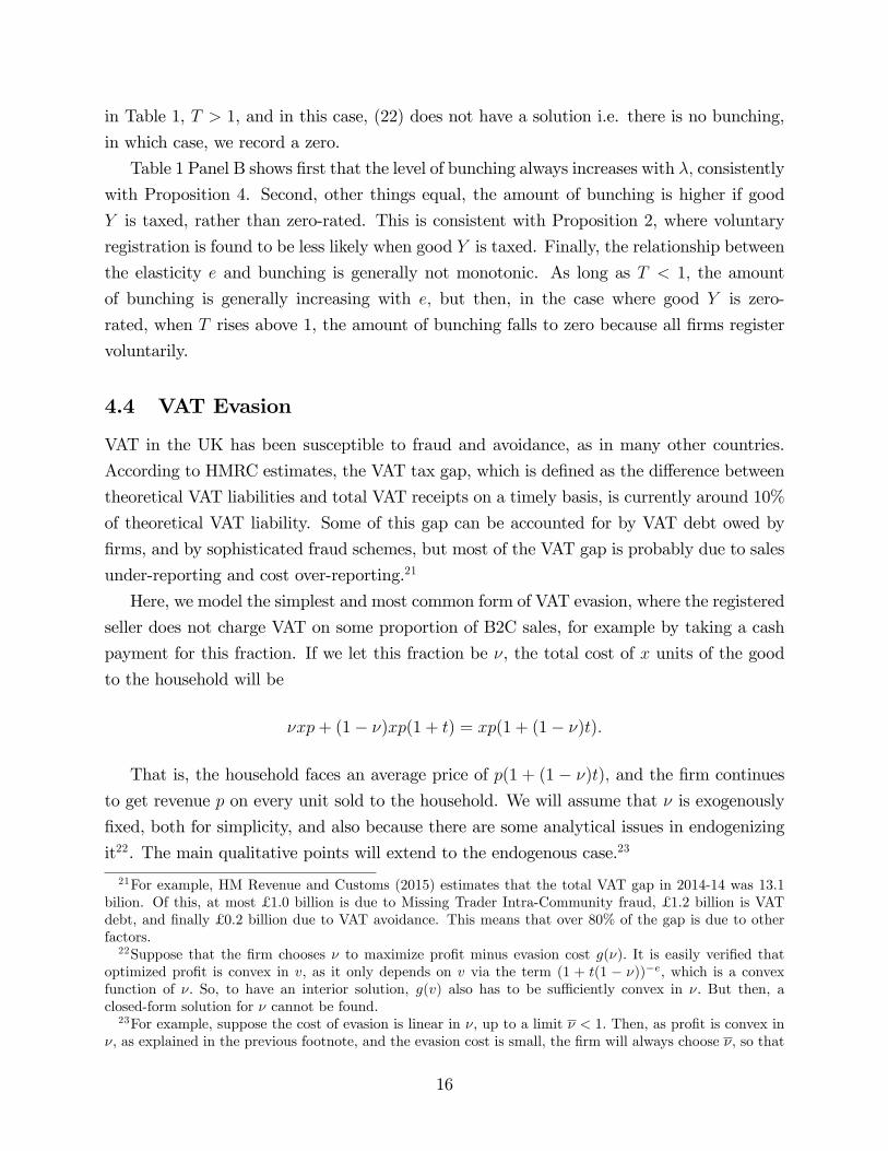
4.4 VAT Evasion

VAT in the UK has been susceptible to fraud and avoidance, as in many other countries.

According to HMRC estimates, the VAT tax gap, which is defined as the difference between

theoretical VAT liabilities and total VAT receipts on a timely basis, is currently around 10%

of theoretical VAT liability. Some of this gap can be accounted for by VAT debt owed by

firms, and by sophisticated fraud schemes, but most of the VAT gap is probably due to sales

under-reporting and cost over-reporting.21

Here, we model the simplest and most common form of VAT evasion, where the registered

seller does not charge VAT on some proportion of B2C sales, for example by taking a cash

payment for this fraction. If we let this fraction be ν, the total cost of x units of the good

to the household will be

νxp+ (1− ν)xp(1 + t) = xp(1 + (1− ν)t).

That is, the household faces an average price of p(1 + (1 − ν)t), and the firm continues

to get revenue p on every unit sold to the household. We will assume that ν is exogenously

fixed, both for simplicity, and also because there are some analytical issues in endogenizing

it22. The main qualitative points will extend to the endogenous case.23

21For example, HM Revenue and Customs (2015) estimates that the total VAT gap in 2014-14 was 13.1bilion. Of this, at most £ 1.0 billion is due to Missing Trader Intra-Community fraud, £ 1.2 billion is VATdebt, and finally £ 0.2 billion due to VAT avoidance. This means that over 80% of the gap is due to otherfactors.22Suppose that the firm chooses ν to maximize profit minus evasion cost g(ν). It is easily verified that

optimized profit is convex in v, as it only depends on v via the term (1 + t(1 − ν))−e, which is a convexfunction of ν. So, to have an interior solution, g(v) also has to be suffi ciently convex in ν. But then, aclosed-form solution for ν cannot be found.23For example, suppose the cost of evasion is linear in ν, up to a limit ν < 1. Then, as profit is convex in

ν, as explained in the previous footnote, and the evasion cost is small, the firm will always choose ν, so that

16

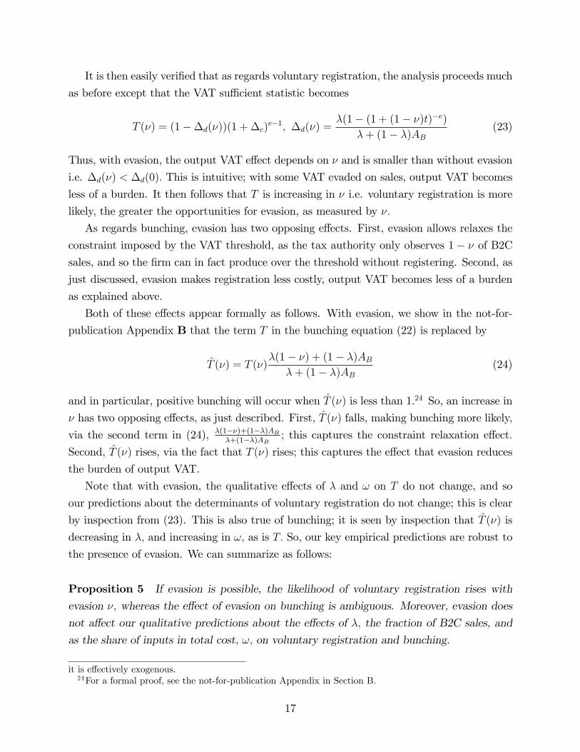
It is then easily verified that as regards voluntary registration, the analysis proceeds much

as before except that the VAT suffi cient statistic becomes

T (ν) = (1−∆d(ν))(1 + ∆c)e−1, ∆d(ν) =

λ(1− (1 + (1− ν)t)−e)

λ+ (1− λ)AB(23)

Thus, with evasion, the output VAT effect depends on ν and is smaller than without evasion

i.e. ∆d(ν) < ∆d(0). This is intuitive; with some VAT evaded on sales, output VAT becomes

less of a burden. It then follows that T is increasing in ν i.e. voluntary registration is more

likely, the greater the opportunities for evasion, as measured by ν.

As regards bunching, evasion has two opposing effects. First, evasion allows relaxes the

constraint imposed by the VAT threshold, as the tax authority only observes 1 − ν of B2Csales, and so the firm can in fact produce over the threshold without registering. Second, as

just discussed, evasion makes registration less costly, output VAT becomes less of a burden

as explained above.

Both of these effects appear formally as follows. With evasion, we show in the not-for-

publication Appendix B that the term T in the bunching equation (22) is replaced by

T (ν) = T (ν)λ(1− ν) + (1− λ)AB

λ+ (1− λ)AB(24)

and in particular, positive bunching will occur when T (ν) is less than 1.24 So, an increase in

ν has two opposing effects, as just described. First, T (ν) falls, making bunching more likely,

via the second term in (24), λ(1−ν)+(1−λ)ABλ+(1−λ)AB

; this captures the constraint relaxation effect.

Second, T (ν) rises, via the fact that T (ν) rises; this captures the effect that evasion reduces

the burden of output VAT.

Note that with evasion, the qualitative effects of λ and ω on T do not change, and so

our predictions about the determinants of voluntary registration do not change; this is clear

by inspection from (23). This is also true of bunching; it is seen by inspection that T (ν) is

decreasing in λ, and increasing in ω, as is T. So, our key empirical predictions are robust to

the presence of evasion. We can summarize as follows:

Proposition 5 If evasion is possible, the likelihood of voluntary registration rises with

evasion ν, whereas the effect of evasion on bunching is ambiguous. Moreover, evasion does

not affect our qualitative predictions about the effects of λ, the fraction of B2C sales, and

as the share of inputs in total cost, ω, on voluntary registration and bunching.

it is effectively exogenous.24For a formal proof, see the not-for-publication Appendix in Section B.

17

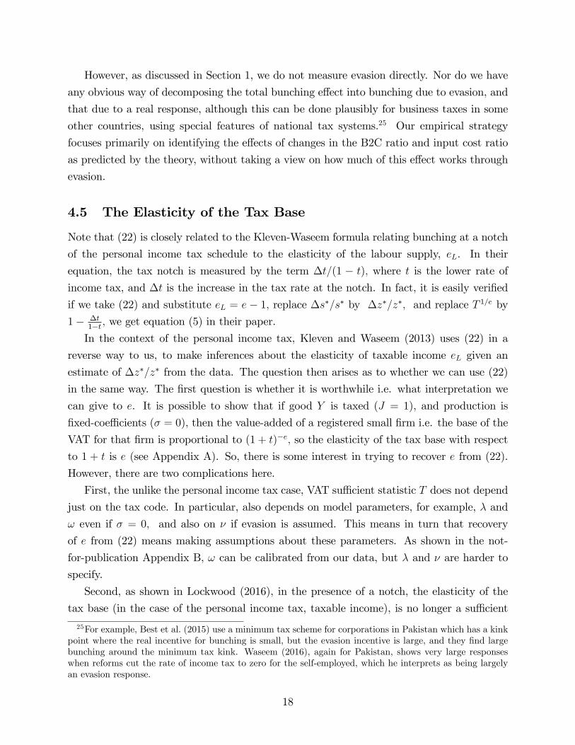
However, as discussed in Section 1, we do not measure evasion directly. Nor do we have

any obvious way of decomposing the total bunching effect into bunching due to evasion, and

that due to a real response, although this can be done plausibly for business taxes in some

other countries, using special features of national tax systems.25 Our empirical strategy

focuses primarily on identifying the effects of changes in the B2C ratio and input cost ratio

as predicted by the theory, without taking a view on how much of this effect works through

evasion.

4.5 The Elasticity of the Tax Base

Note that (22) is closely related to the Kleven-Waseem formula relating bunching at a notch

of the personal income tax schedule to the elasticity of the labour supply, eL. In their

equation, the tax notch is measured by the term ∆t/(1 − t), where t is the lower rate of

income tax, and ∆t is the increase in the tax rate at the notch. In fact, it is easily verified

if we take (22) and substitute eL = e − 1, replace ∆s∗/s∗ by ∆z∗/z∗, and replace T 1/e by

1− ∆t1−t , we get equation (5) in their paper.

In the context of the personal income tax, Kleven and Waseem (2013) uses (22) in a

reverse way to us, to make inferences about the elasticity of taxable income eL given an

estimate of ∆z∗/z∗ from the data. The question then arises as to whether we can use (22)

in the same way. The first question is whether it is worthwhile i.e. what interpretation we

can give to e. It is possible to show that if good Y is taxed (J = 1), and production is

fixed-coeffi cients (σ = 0), then the value-added of a registered small firm i.e. the base of the

VAT for that firm is proportional to (1 + t)−e, so the elasticity of the tax base with respect

to 1 + t is e (see Appendix A). So, there is some interest in trying to recover e from (22).

However, there are two complications here.

First, the unlike the personal income tax case, VAT suffi cient statistic T does not depend

just on the tax code. In particular, also depends on model parameters, for example, λ and

ω even if σ = 0, and also on ν if evasion is assumed. This means in turn that recovery

of e from (22) means making assumptions about these parameters. As shown in the not-

for-publication Appendix B, ω can be calibrated from our data, but λ and ν are harder to

specify.

Second, as shown in Lockwood (2016), in the presence of a notch, the elasticity of the

tax base (in the case of the personal income tax, taxable income), is no longer a suffi cient

25For example, Best et al. (2015) use a minimum tax scheme for corporations in Pakistan which has a kinkpoint where the real incentive for bunching is small, but the evasion incentive is large, and they find largebunching around the minimum tax kink. Waseem (2016), again for Pakistan, shows very large responseswhen reforms cut the rate of income tax to zero for the self-employed, which he interprets as being largelyan evasion response.

18

statistic for the marginal deadweight loss of the tax, so elasticity estimates are of less interest

from a normative point of view. So, for these reasons, we do not attempt elasticity estimates.

4.6 Summary of Theoretical Results

We now summarize the theoretical results in Figure 2, which shows how firms of productivity

type a behave as T varies. The figure is drawn under the simplifying assumption that eC = eB

and that there is no evasion. In this case, we know that all firms register for VAT if T > 1.

So, all firms with a > a∗ are registered with a turnover above the threshold, but all firms

with a < a∗ are voluntarily registered, where a∗ is defined in (18) above.

When T falls below 1, firms a ∈ [a∗, a∗+∆a∗] start to bunch at the registration threshold.

as T falls, this bunching interval becomes larger. So, for any fixed value of T, firms can now

be in one of three regimes: when a is low, the firm will be unconstrained but below the

threshold, when a is high, the firm will be unconstrained and above the threshold and thus

registered, and when a is intermediate, the firm will be just at the threshold.

It is also clear from Figure 2 how voluntary registration and bunching may coexist in any

given industry. Some fraction of firms may have a T > 1, so the lower-productivity ones in

this group will be voluntarily registered. At the same time, some other fraction may have a

T < 1, so some of this latter group will be bunching.

5 Context and Data

5.1 The Value-Added Tax System in the UK

The Value-Added tax in the UK is remitted by approximately 2 million registered businesses

in each fiscal year. It is the third largest source of government revenue following income tax

and national insurance contributions. In 2011/12, VAT raised £ 98.2 billion, accounting for

21.1% of total tax revenue and 6.5% of GDP in the UK.26

VAT is levied on most goods and services provided by registered businesses in the UK,

goods and some services imported from countries outside the European Union (EU), and

brought into the UK from other EU countries. All businesses must register for VAT if their

taxable turnover is above a given threshold.27 A VAT registered business pays VAT on its

purchases (input tax), and charges VAT on the full sale price of the taxable supplies (output

26See http://www.hmrc.gov.uk/stats/tax receipts/tax-receipts-and-taxpayers.pdf.27VAT taxable turnover includes the value of any goods or services a business supplies within the UK,

unless they are exempt from VAT. Any supplies that would be zero-rated for VAT are included as part ofthe taxable turnover.

19

tax). Businesses can also choose to register voluntarily with a turnover below the threshold

in order to recover the input taxes.

The default VAT rate is the standard rate, which was 17.5% between April 1, 2004 and

December 1, 2008 and was temporarily reduced to 15% before January 1, 2010. The standard

rate was then reverted to 17.5% until 4 January 2011 when it was increased to 20% and has

been at that rate since. A small number of goods and services have VAT levied at a reduced

rate of 5% and there are also goods and services that are charged at a zero rate or are

exempt from VAT altogether.28. Neither businesses that make zero-rate or exempt supplies

charge output VAT to the customers, and the key difference between them is that input tax

cannot be claimed against output tax on exempted supplies. The registration thresholds and

standard rate of VAT over our sample period are shown in Table 2

The increase in registration threshold tracks the rate of inflation.29 The UK has the

highest registration threshold in the EU, which is perceived as a way for the government to

reduce the compliance costs of small businesses not wishing to register for VAT.30

There are two rules governing registration, a forward-looking rule and a backward-looking

one. Under the forward-looking rule, a firm must also register for VAT if its VAT taxable

turnover is likely to go over the threshold in the next 30 days. Under the backward-looking

rule, a firm must register if its VAT-taxable turnover in the previous 12 months was above

the threshold. Strictly speaking, our theoretical model is static and applies to the forward-

looking decision; that is, the firm must register if turnover in the current year is expected to

exceed the threshold. In our sample, around 68% of first-time registers have a previous-year

turnover less than the VAT threshold. This suggests that the forward-looking decision is

more important.

5.2 Data

We construct our dataset by linking the universe of VAT returns to the universe of corpora-

tion tax records in the UK. The first data set provides detailed information for businesses in

28A reduced rate of 5% is charged on a small number of supplies under schedule 7A of the Value AddedTax Act (VATA) 1994. Principally, they include the supply of domestic fuel and power, the installation ofenergy saving materials, women’s sanitary products, children’s car seats and certain types of constructionwork.29Specifically, under Article 24(2)(c) of the sixth EC VAT directive (77/388/EEC 17 May 1977). These

provisions are now consolidated in the principal VAT directive (2006/112/EC); article 287 allows for Statesto increase the registration threshold in line with inflation. As far as we are aware, there is no interactionbetween the VAT registration threshold with other major taxes in the UK, not does it change the probabilityof being audited for firms around the threshold.30Small firms with annual taxable turnover of up to £ 150,000 can use a simplified flat-rate VAT scheme,

but are subject to the same registration threshold. The flat-rate scheme is not widely used. In 2007, only16% of eligible firms were registered under the flat-rate scheme (Vesal, 2013).

20

different legal forms including sole traders, partnerships, and companies that are registered

for VAT. To obtain information on non-VAT registered businesses, we link the VAT records

to the population of corporation tax records based on a common anonymised taxpayer ref-

erence number. The linked dataset allows us to identify both registers and non-registers for

the population of UK companies, and contains rich information on VAT and corporation tax

for each company and year.

We further merge the linked tax dataset with two additional data sources: (1) the FAME

(Financial Analysis Made Easy) annual company account database for additional firm char-

acteristics and accounting information and (2) the annual sector-level statistics on the share

of sales to final consumers based on the Offi ce of National Statistics (ONS) Input-Output

Tables. The last data source gives us an empirical proxy for λ, the share of sales that are

B2C at the 2-digit SIC industry level.

The final dataset contains 731,706 observations for 435,688 companies between April 1,

2004 and March 30, 2010.31 For each company-year observation, we have information on the

VAT-exclusive turnover taken from the corporate tax records, and whether the company is

registered for VAT.32We examine a few key factors that drive firms’decisions about voluntary

registration, including the share of input cost relative to total turnover (input-cost ratio),

the share of sales to final consumers (B2C sales ratio), firm-specific history of registration,

and the degree of industry-level competitiveness (measured by four-firm concentration ratio,

or CR4)33.31We take several steps to refine the sample to study the VAT registration decisions of individual companies.

First, we eliminate companies which are part of a larger VAT group and focus only on standalone independentcompanies. This is because companies under common control—for example, subsidiaries of a parent company—can register as a VAT group and submit only one VAT return for all companies in a VAT group.Second, we drop all observations with partial-year tax or accounting records because the registration

decision can be based on turnover in the previous 12 months. We further eliminate companies that mainlyengage in overseas activities based on the HMRC trade classification. This is because the taxable VATturnover is based on sales of goods and services within the UK. Finally, we drop companies with an effectiverate of VAT that is less than 10%, where the effective rate is the output VAT relative to VAT-eligible salesfor registered companies, to form the main sample for empirical analysis. Empirical results based on thefull sample that include all firms with an effective VAT rate below 10% are quantitatively similar to thoseobtained using the main sample and are available upon request.32Our empirical analysis is based on turnover reported in the CT600 for two reasons. The first is mechan-

ical: we only observe turnover liable for VAT for firms that are registered. The second is related to saliencegiven that firms that are not registered for VAT are more likely to base their registration decision on theoverall amount of turnover, instead of computing a separate measure of turnover that is subject to VAT. Tosee whether this is true, we predict (out-of-sample) the amount of turnover liable for VAT for unregisteredfirms, by regressing the amount of turnover liable for VAT on the amount of total turnover and a full set ofindustry and year dummies. We then plot a similar histogram of turnover as in Figure 2 Panel B based onactual/predicted turnover liable for VAT for registered/unregistered firm. Bunching below the VAT notchis still present, but much more noisy and imprecise comparing to bunching based on total turnover reportedin CT600. The empirical differences suggest that for unregistered firms, they are more likely to rely on theoverall turnover figure for their VAT registration decisions.33We calculate the concentration ratio based on the market shares of the four largest firms in an industry,

21

We use two different data sets to test related hypotheses developed in Section 3. First,

we use all the firms with turnover below the current-year VAT registration threshold to

examine the choice of voluntary registration. We say that a firm is voluntarily registered if

it has never registered before and has a turnover below the VAT threshold, or that if it was

registered in the previous year and has a turnover below the VAT deregistration threshold.

In the main sample, 62.5% of firms have a turnover below the VAT threshold, and of these,

44.1% of them are registered for VAT. So, overall, 27.6% of firms in the main sample of

companies are voluntarily registered. Second, we focus on firms with turnover within the

neighboring of the registration threshold, i.e. between £ 10,000 and £ 200,000, to analyze the

extent of bunching below the VAT notch.

5.3 Summary Statistics

Figure 3 presents convincing evidence that the VAT registration threshold is binding in the

UK, by showing a histogram of the normalized turnover by pooling data between 2004/05

and 2009/10, where the normalized turnover is defined as firms’nominal turnover net of

the current-year VAT notch. There is an evident excess of mass just below the notch and a

small missing mass above, in the otherwise smooth distribution of turnover. However, it is

worth noting that relative to some other studies, the excess mass below the threshold is not

sharply bunched at the notch. A plausible explanation is that firms have less control over

their turnover than individuals do over their earnings for example. Alternatively, firms that

benefit from voluntary registration can also stay below the registration threshold.

Table 3 reports summary statistics for companies in the neighborhood of current-year

VAT notch, i.e. those with nominal turnover of between £ 10,000 and £ 200,000. The first

three columns report the mean, standard deviation and the number of non-missing obser-

vations for the key variables used in empirical analysis. Companies in this turnover region

account for around 52.94% of all companies in the linked dataset. Columns (4)-(6) focus

on the registered companies while columns (7)-(9) focus on the non-registered. The last

two columns test whether there is any significant difference between the means of the two

groups, by reporting the t−statistic and the corresponding p-value in columns (9) and (10),respectively.

based on the larger dataset of population of corporate tax records.

22

6 Voluntary Registration

6.1 Evidence on Voluntary Registration

In this section, we examine whether the decision of voluntary registration is consistent with

the theory in the three key aspects as predicted by Proposition 2, including whether a firm

is more likely to voluntarily register for VAT if it mainly sells to final consumers, has a larger

share of inputs in cost, or in a more competitive industry.

We first note in Table 4 that the empirical pattern is broadly consistent with Proposition

2. As the share of B2C sales falls, i.e. when moving from the fourth (Q4) to the first quartile

(Q1), the share of voluntarily registered firms tends to rise. Similarly, as the input cost ratio

rises, the share of voluntarily registered firms tends to increase.

Next, we model the decision of voluntary registration in a binary choice model of the

following form:

Rit = γ1 + γ2B2Cj(i) + γ3ICRit + γ4CR4j(i) + γ5Xit + ρt + φi + υit, (25)

where Rit is a dummy indicator that takes value 1 if the firm is voluntarily registered and zero

otherwise. The key variables of interest are B2Cj(i), the industry-level B2C ratio for firm i

(that is, firm i in industry j(i)), ICRit, the input cost ratio for firm i in year t, and CR4j(i),

the four-firm concentration ratio to measure competition in industry j in which firm i is

located. Xit are other firm-level controls, φi and ρt are time-invariant firm fixed effects and

year dummies, and υit is the error term. We estimate equation (25) in a linear probability

framework based on the standard OLS assumptions and in a fixed-effect logit model. The

regression sample includes all firms with turnover below the current-year VAT registration

threshold. Consistent with Proposition 2, we expect that γ2 > 0, γ3 > 0, whereas the sign

of γ4 is uncertain.

Table 5 reports the estimation results from the linear probability model.34 Columns

(1)-(3) includes each of the key variables at a time, and column (4) includes all three key

variables in the regression. Without inclusion of firm fixed effects, we can examine the effect

of industry-level B2C sales ratio and CR4 ratio on the probability of voluntary registration

in the first four columns. The coeffi cient estimates are negative and statistically significant,

indicating that the likelihood to voluntarily register for VAT is reduced by around 4 percent-

age points given a one-standard-deviation increase in the B2C sales ratio, and by around 0.2

to 1 percentage point given a one-standard-deviation increase in the CR4 ratio.

34The estimation results from the fixed-effects logit model are very similar and available from the authorsupon request.

23

The rest of columns add firm fixed effects and the coeffi cients on the B2C and CR4 ratios

are often imprecisely estimated due to limited time-series variation at the industry level. For

comparison, column (5) does not include any additional controls, whereas column (6) adds

firm-level trading profit and age since incorporation. Columns (7) checks the robustness of

the results by replacing the salary-inclusive input cost ratio calculated from the corporation

tax records with the salary-exclusive input cost ratio calculated from FAME. The latter

improves precision in the measurement of input cost, but substantially reduces the sample

size given that few firms report the direct cost of sales. The coeffi cient estimate for the input

cost ratio remains positive and highly significant throughout the different specifications.

Moreover, the coeffi cient estimates for the B2C sales ratio and CR4 ratio are negative and

significant at 10% level in column (7). Focusing on results in columns (4) and (7), the

likelihood of voluntarily registering for VAT is increased by around 1 percentage point given

a one standard deviation increase in the input cost ratio.

7 Evidence on Bunching

7.1 Estimation Methodology

As set out in the conceptual framework in Section 3, the VAT registration threshold at

the cutoff turnover value s∗ will induce excess bunching at the threshold by companies for

which voluntary registration is not optimal. We are interested in constructing the empirical

equivalent of∆s∗/s∗. First, we measure∆s∗, the amount of excess bunching, as the difference

between the observed and predicted bin counts over the excluded range that falls below the

VAT notch:

∆s∗ =s∗∑

i=s∗−

(cj − cj).

Here, cj is the actual number of firms in each £ 100 turnover bin, and cj is the counterfactual

bin counts without the notch. The range(s∗−, s

∗+

)specifies turnover bins around the notch

where bunching occurs and are therefore excluded from predicting the counterfactual distri-

bution. Specifically, the lower bound of the excluded turnover region, s∗−, is set at the point

where excess bunching starts. The upper bound of the excluded region, s∗+, is estimated in

an iteration procedure to ensure that the excess mass below the VAT notch is equal to the

missing mass above.35 We then measure the amount of bunching by b = ∆s∗/s∗, where s∗ is

simply the VAT threshold for that year.

35We follow the standard procedure to estimate the counterfactual distribution. By grouping companiesinto small turnover bins of £ 100, we estimate the counterfactual distribution around the VAT notch s∗ in

24

7.2 Bunching Evidence

7.2.1 Baseline Estimates

This section presents evidence of bunching below the VAT notch using the main sample

of companies with turnover between £ 10,000 and £ 200,000. Figure 4 presents bunching

around the threshold in each financial year between 2004/05 and 2009/10. Panel A shows the

empirical distribution of turnover (blue dots) as a histogram in £ 1,000 bins and the estimated

counterfactual distribution (red line) in 2004-05. Each dot denotes the upper bound of a given

bin and represents the number of companies in each turnover bin of £ 1,000. Similar to Chetty

et al. (2011) and Kleven and Waseem (2013), we estimate the counterfactual distribution by

fitting a flexible polynomial of order 3 to the empirical distribution, excluding firms in the

excluded range close to the VAT notch.36 The lower bound of the excluded turnover range

is demarcated by the vertical dashed line and the VAT notch demarcated by the vertical

solid line.37 The next five panels focus on subsequent years during which the VAT notch was

increased annually to track inflation. Each panel reports the estimated bunching ratio (b)

and its standard error in in parenthesis.

Three main findings are worth noting in Figure 4. First, the VAT notch creates evident

bunching below the threshold. Excess bunching ranges from 0.82 to 1.29 times the height

of the counterfactual distribution, and is strongly significant in all years during the sample

period.38 Second, excess bunching tracks precisely the annual change in the nominal VAT

notch due to adjustment to inflation. In each year the excess bunching is concentrated within

£ 2,000 below the VAT. Third, in contrast with the large bunching below the threshold, there

is a small hole in the distribution above the VAT notch. The range of the hole spans from

£ 8,500 to £ 15,000 above the cutoff, although we do not attempt to estimate the magnitude

of optimization frictions implied by the hole given the various reason discussed in section 3.

the following regression:

cj =

q∑l=0

βi (sj)l+

s∗+∑i=s∗−

γiI {j = i}+ εj , (26)

where cj is the number of companies in turnover bin j, sj is the distance between turnover bin j and theVAT notch s∗, q is the order of the polynomial, and I {·} is an indicator function. The error term εj reflectsmisspecification of the density equation.36As a robustness check we have tried values between 3 and 5 for the order of the polynomial and our

results are not significantly changed.37The upper bound of the excluded turnover region is estimated in an iteration procedure to ensure that

the area under the estimated counterfactual density is equal the area under the observed density.38Unlike to studies analysing bunching in the taxable income of individuals (Kleven and Waseem (2013))

and corporations (Devereux, Liu and Loretz (2014)), we do not find any evident bunching at round numbers.The absence of round-number bunching suggests that firms have less control over their turnover than reportedtaxable earnings.

25

In Kleven (2016), it is argued that in the context of the personal income tax, bunching

is much more likely to be due evasion, rather than to real earnings responses. Here, as

already noted, both evasion and real responses may be driving observed bunching. Our

main approach is not to try to decompose observed bunching into a real and evasion part,

but just to note that our theory, which includes an evasion element, makes predictions about

how bunching will vary with the share of B2C sales and the input cost ratio, and we turn to

this next. However, in Section 7.2.3 below, we do address the evasion issue, and show some

evidence that bunching may partly be due to turnover misreporting.

7.2.2 Heterogeneity in Bunching

We have shown a stable distribution of turnover throughout the entire period 2004/05-

2009/10, with an evident and persistent bunching of companies below the VAT notch in

each year. We now explore potential heterogeneity in bunching to see whether the empirical

pattern is consistent with the predictions set out in Proposition 3, that firms are more likely

to bunch below the VAT notch if the share of B2C sales is high, or the share of input costs

is low. We will also investigate the effect of the level of competition in the industry where

the firm is located, although that is predicted to have an ambiguous effect theoretically.

First, we explore how companies with different B2C sales ratio respond to the same VAT

notch by dividing companies into four groups according to the quartiles of B2C sales ratio.

We estimate annual bunching ratios separately for each quartile, and plot the point estimate

of the bunching ratio with the corresponding 95% confidence intervals in Figure 5. There

are two interesting findings in Figure 5. First, all bunching estimates are positive and highly

significant, even in the lowest B2C quartile where on average between 0.3% and 25.4% of

sales are B2C. Second, there is a clear pattern that the estimated bunching ratio increases

with quartiles of the B2C sales ratio. In particular, the estimated bunching ratio for firms

in the top quartile is significantly larger than for firms in the bottom quartile. The observed

strong aggregate bunching is mainly driven by the behavioral responses of companies in the

3rd and 4th quartile of the B2C sales ratio.

To explore how companies with different shares of direct input cost respond to the same

VAT notch, we construct a firm-specific measure of average input-cost ratio during the

sample period and divide all companies into four groups according to the quartiles of input-

cost ratio. We obtain information on direct cost of sales excluding salary from company

accounts in FAME and since it is optional for small and medium-sized companies to disclose

this information, only 12.52% of companies in the estimation sample report a non-missing

direct cost of sales. To increase effi ciency of the empirical test, we pool observations with non-

missing input cost in all years and present bunching evidence with respect to the normalized

26

VAT notch in Figure 6.

Panel A compares the empirical distributions of companies around the normalized VAT

notch across quartiles of the input-cost ratio. It presents clear evidence that the degree

of bunching decreases with the input-cost ratio. The distribution of companies in the top

quartile is quite smooth around the normalized VAT notch, while distributions of companies

in the lower quartiles all exhibit some degree of bunching just below the VAT notch. Panel B

quantifies the difference in the extent of bunching by plotting the estimated bunching ratio

with the corresponding 95% confidence interval for each input-cost ratio quartile. Quantitat-

ively, the bunching estimate is very small and insignificant for companies in the top quartile

of the input-cost ratio distribution. In contrast, the bunching estimates for companies in the

lower quartiles of the input-cost ratio are positive and highly significant.

Finally, we examine the extent of bunching depending on the degree of competition in

the product market. We measure competition at the industry level using the four-firm

concentration ratio (CR4), so a high CR4 is associated with a lower level of competition.

As in the previous cases, we examine how bunching varies across quartiles of the CR4 ratio

in Figure 7. Panel A demonstrates that bunching clearly increases as the CR4 increases,

whereas Panel B quantifies the difference in the extent of bunching by plotting the bunching

estimates with the corresponding 95% confidence interval. All the bunching estimates are

significantly different from zero, and there is an substantial increase in the degree of bunching

at the third and fourth quartile of the CR4 ratio where there is less competition in the product

market.

7.2.3 Bunching via Turnover Misreporting

In this section, we provide some suggestive evidence on the extent of bunching due to turnover

misreporting. When bunching is due to a decrease in real output, we expect companies to

reduce their input costs in proportion, so that the distribution of input-cost ratio for non-

registered companies should be smooth around the VAT notch. When bunching is due to

turnover misreporting, we conjecture that the non-registered companies are less likely to

under-report their input costs and wage expenses. Both costs are deductible for corporation

taxes and the latter is subject to third-party reporting. In other words, the gain from under-

reporting the deductible costs is considerably smaller than the gain from under reporting

the turnover to avoid VAT registration. If the majority of companies bunch via turnover

misreporting, we would expect to see a higher average input-cost ratio for the non-registered

group just below the VAT notch, relative to that for the registered group.

Figure 8 pools all observations in the sample period and plots the distribution of av-

erage input-cost ratio for registered and non-registered companies in £ 1,000 turnover bins,

27

respectively. In Panel A, the input-cost ratio is salary exclusive and represents the share of

direct cost of sales relative to total turnover. The solid blue line shows the average input

cost relative to sales for registered companies within each turnover bin of £ 1,000 normalized

by the current-year VAT notch, and the dashed blue line shows the average input cost ra-

tio for the unregistered companies. Consistent with the theory, voluntary registers incur a

much larger input cost as indicated by their average input-cost ratio which is consistently

larger than that for the non-registered companies below the VAT notch. On the other hand,

there is no evident increase in the average input-cost ratio just below the VAT notch for the

non-registered group. The distribution is relatively smooth and continues to increase with

turnover above the VAT notch.

In comparison, Panel B plots the distribution of average input-cost ratio inclusive of

salary, for registered and non-registered companies, respectively. There is striking difference

between the two input-cost ratio series just below the VAT notch. The two series move in

parallel directions until the average input-cost ratio for the non-registered companies starts to

increase drastically just below the VAT notch. The sharp increase in the salary-inclusive cost

ratio can be partly attributed to the fixed nature of salary cost which takes longer to adjust

than variable costs of input. On the other hand, the sharp increase is also consistent with

the fact that salary is subject to third-party reporting and thus it is more costly/diffi cult for

small businesses to underreport salary expenses. Overall, Panel A and B in Figure 8 provide

suggestive yet not conclusive evidence that part of bunching is due to turnover misreporting.

8 Evidence on Dynamics

One limitation of our study so far is that we do not consider dynamic behavior of firms.

Changing registration status involves some cost to the firm. This raises the possibility, in

particular, that firms who were initially above the registration threshold and fall below may

stay registered, simply because of the cost of deregistration. So, some of the firms who seem

to be voluntary registered may just be behaving in this way because of inertia.

In this section, we investigate the importance of inertia in driving VAT registration by

analyzing the dynamic behavior of firms when they cross registration and deregistration

thresholds. First, we compute a transition probability matrix for firms moving between

registration states in Table C.1, which shows the probability of being registered or not

registered t years after initially being in a given state.39 For example, the entry in the

first cell of the matrix, 89.3%, shows that of all the firms that where initially registered in

39Changes in the transition probability could also driven by attrition, therefore we focus on a balancedsample of firms that we observe throughout the sample period.

28

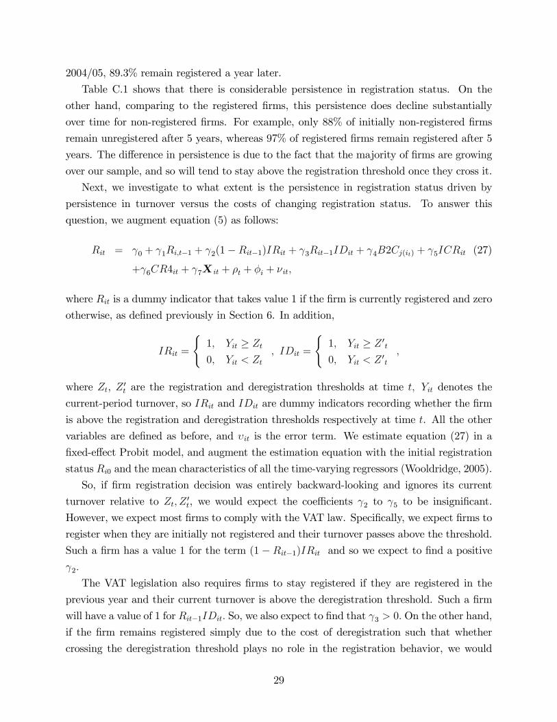
2004/05, 89.3% remain registered a year later.

Table C.1 shows that there is considerable persistence in registration status. On the

other hand, comparing to the registered firms, this persistence does decline substantially

over time for non-registered firms. For example, only 88% of initially non-registered firms

remain unregistered after 5 years, whereas 97% of registered firms remain registered after 5

years. The difference in persistence is due to the fact that the majority of firms are growing

over our sample, and so will tend to stay above the registration threshold once they cross it.

Next, we investigate to what extent is the persistence in registration status driven by

persistence in turnover versus the costs of changing registration status. To answer this

question, we augment equation (5) as follows:

Rit = γ0 + γ1Ri,t−1 + γ2(1−Rit−1)IRit + γ3Rit−1IDit + γ4B2Cj(it) + γ5ICRit (27)

+γ6CR4it + γ7X it + ρt + φi + νit,

where Rit is a dummy indicator that takes value 1 if the firm is currently registered and zero

otherwise, as defined previously in Section 6. In addition,

IRit =

{1, Yit ≥ Zt

0, Yit < Zt, IDit =

{1, Yit ≥ Z ′t

0, Yit < Z ′t,

where Zt, Z ′t are the registration and deregistration thresholds at time t, Yit denotes the

current-period turnover, so IRit and IDit are dummy indicators recording whether the firm

is above the registration and deregistration thresholds respectively at time t. All the other

variables are defined as before, and υit is the error term. We estimate equation (27) in a

fixed-effect Probit model, and augment the estimation equation with the initial registration

status Ri0 and the mean characteristics of all the time-varying regressors (Wooldridge, 2005).

So, if firm registration decision was entirely backward-looking and ignores its current

turnover relative to Zt, Z ′t, we would expect the coeffi cients γ2 to γ5 to be insignificant.

However, we expect most firms to comply with the VAT law. Specifically, we expect firms to

register when they are initially not registered and their turnover passes above the threshold.

Such a firm has a value 1 for the term (1 − Rit−1)IRit and so we expect to find a positive

γ2.

The VAT legislation also requires firms to stay registered if they are registered in the

previous year and their current turnover is above the deregistration threshold. Such a firm

will have a value of 1 for Rit−1IDit. So, we also expect to find that γ3 > 0. On the other hand,

if the firm remains registered simply due to the cost of deregistration such that whether

crossing the deregistration threshold plays no role in the registration behavior, we would

29

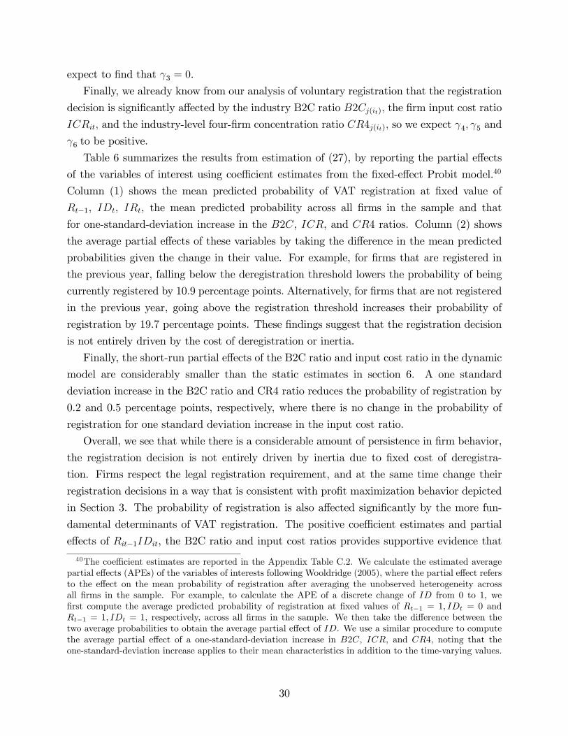
expect to find that γ3 = 0.

Finally, we already know from our analysis of voluntary registration that the registration

decision is significantly affected by the industry B2C ratio B2Cj(it), the firm input cost ratio

ICRit, and the industry-level four-firm concentration ratio CR4j(it), so we expect γ4, γ5 and

γ6 to be positive.

Table 6 summarizes the results from estimation of (27), by reporting the partial effects

of the variables of interest using coeffi cient estimates from the fixed-effect Probit model.40

Column (1) shows the mean predicted probability of VAT registration at fixed value of

Rt−1, IDt, IRt, the mean predicted probability across all firms in the sample and that

for one-standard-deviation increase in the B2C, ICR, and CR4 ratios. Column (2) shows

the average partial effects of these variables by taking the difference in the mean predicted

probabilities given the change in their value. For example, for firms that are registered in

the previous year, falling below the deregistration threshold lowers the probability of being

currently registered by 10.9 percentage points. Alternatively, for firms that are not registered

in the previous year, going above the registration threshold increases their probability of

registration by 19.7 percentage points. These findings suggest that the registration decision

is not entirely driven by the cost of deregistration or inertia.

Finally, the short-run partial effects of the B2C ratio and input cost ratio in the dynamic

model are considerably smaller than the static estimates in section 6. A one standard

deviation increase in the B2C ratio and CR4 ratio reduces the probability of registration by

0.2 and 0.5 percentage points, respectively, where there is no change in the probability of

registration for one standard deviation increase in the input cost ratio.

Overall, we see that while there is a considerable amount of persistence in firm behavior,

the registration decision is not entirely driven by inertia due to fixed cost of deregistra-

tion. Firms respect the legal registration requirement, and at the same time change their

registration decisions in a way that is consistent with profit maximization behavior depicted

in Section 3. The probability of registration is also affected significantly by the more fun-

damental determinants of VAT registration. The positive coeffi cient estimates and partial

effects of Rit−1IDit, the B2C ratio and input cost ratios provides supportive evidence that

40The coeffi cient estimates are reported in the Appendix Table C.2. We calculate the estimated averagepartial effects (APEs) of the variables of interests following Wooldridge (2005), where the partial effect refersto the effect on the mean probability of registration after averaging the unobserved heterogeneity acrossall firms in the sample. For example, to calculate the APE of a discrete change of ID from 0 to 1, wefirst compute the average predicted probability of registration at fixed values of Rt−1 = 1, IDt = 0 andRt−1 = 1, IDt = 1, respectively, across all firms in the sample. We then take the difference between thetwo average probabilities to obtain the average partial effect of ID. We use a similar procedure to computethe average partial effect of a one-standard-deviation increase in B2C, ICR, and CR4, noting that theone-standard-deviation increase applies to their mean characteristics in addition to the time-varying values.

30

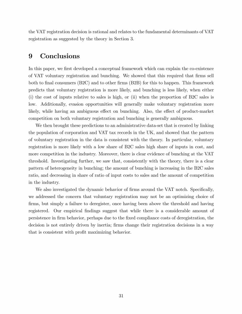
the VAT registration decision is rational and relates to the fundamental determinants of VAT

registration as suggested by the theory in Section 3.

9 Conclusions

In this paper, we first developed a conceptual framework which can explain the co-existence

of VAT voluntary registration and bunching. We showed that this required that firms sell

both to final consumers (B2C) and to other firms (B2B) for this to happen. This framework

predicts that voluntary registration is more likely, and bunching is less likely, when either

(i) the cost of inputs relative to sales is high, or (ii) when the proportion of B2C sales is

low. Additionally, evasion opportunities will generally make voluntary registration more

likely, while having an ambiguous effect on bunching. Also, the effect of product-market

competition on both voluntary registration and bunching is generally ambiguous.

We then brought these predictions to an administrative data-set that is created by linking

the population of corporation and VAT tax records in the UK, and showed that the pattern

of voluntary registration in the data is consistent with the theory. In particular, voluntary

registration is more likely with a low share of B2C sales high share of inputs in cost, and

more competition in the industry. Moreover, there is clear evidence of bunching at the VAT

threshold. Investigating further, we saw that, consistently with the theory, there is a clear

pattern of heterogeneity in bunching; the amount of bunching is increasing in the B2C sales

ratio, and decreasing in share of ratio of input costs to sales and the amount of competition

in the industry.

We also investigated the dynamic behavior of firms around the VAT notch. Specifically,

we addressed the concern that voluntary registration may not be an optimizing choice of

firms, but simply a failure to deregister, once having been above the threshold and having

registered. Our empirical findings suggest that while there is a considerable amount of

persistence in firm behavior, perhaps due to the fixed compliance costs of deregistration, the

decision is not entirely driven by inertia; firms change their registration decisions in a way

that is consistent with profit maximizing behavior.

31

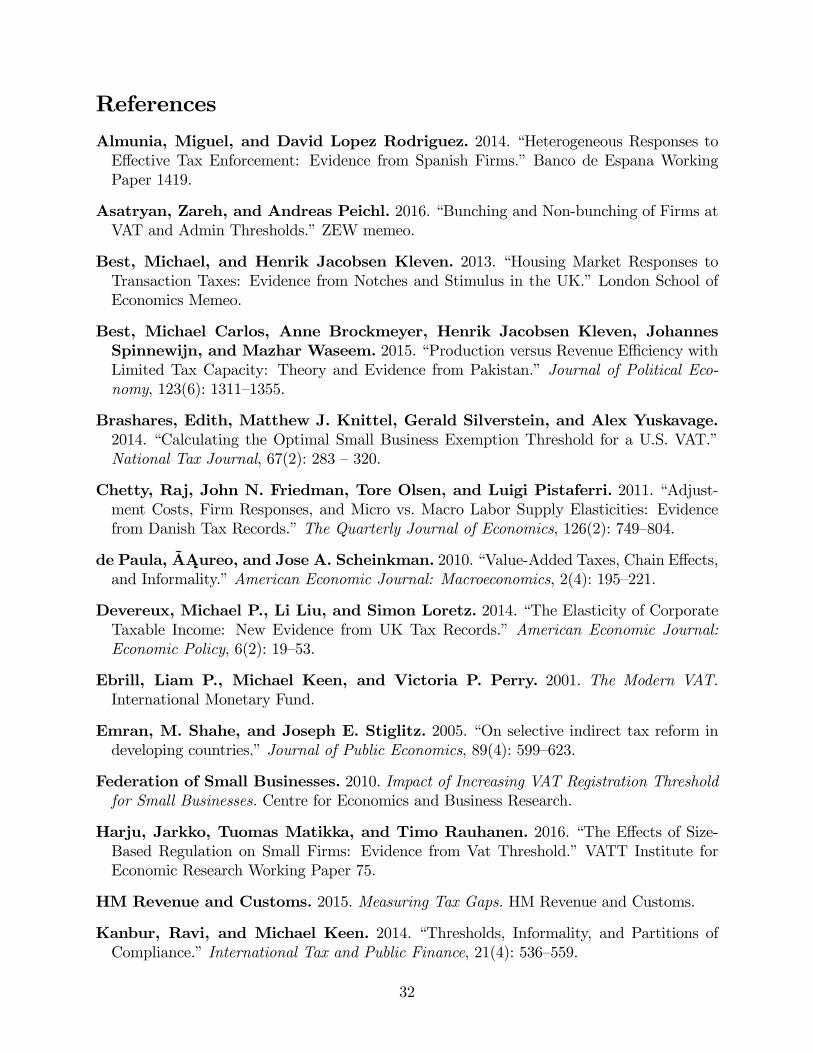
References

Almunia, Miguel, and David Lopez Rodriguez. 2014. “Heterogeneous Responses toEffective Tax Enforcement: Evidence from Spanish Firms.”Banco de Espana WorkingPaper 1419.

Asatryan, Zareh, and Andreas Peichl. 2016. “Bunching and Non-bunching of Firms atVAT and Admin Thresholds.”ZEW memeo.

Best, Michael, and Henrik Jacobsen Kleven. 2013. “Housing Market Responses toTransaction Taxes: Evidence from Notches and Stimulus in the UK.”London School ofEconomics Memeo.

Best, Michael Carlos, Anne Brockmeyer, Henrik Jacobsen Kleven, JohannesSpinnewijn, and Mazhar Waseem. 2015. “Production versus Revenue Effi ciency withLimited Tax Capacity: Theory and Evidence from Pakistan.” Journal of Political Eco-nomy, 123(6): 1311—1355.

Brashares, Edith, Matthew J. Knittel, Gerald Silverstein, and Alex Yuskavage.2014. “Calculating the Optimal Small Business Exemption Threshold for a U.S. VAT.”National Tax Journal, 67(2): 283 —320.

Chetty, Raj, John N. Friedman, Tore Olsen, and Luigi Pistaferri. 2011. “Adjust-ment Costs, Firm Responses, and Micro vs. Macro Labor Supply Elasticities: Evidencefrom Danish Tax Records.”The Quarterly Journal of Economics, 126(2): 749—804.

de Paula, ÃAureo, and Jose A. Scheinkman. 2010. “Value-Added Taxes, Chain Effects,and Informality.”American Economic Journal: Macroeconomics, 2(4): 195—221.

Devereux, Michael P., Li Liu, and Simon Loretz. 2014. “The Elasticity of CorporateTaxable Income: New Evidence from UK Tax Records.”American Economic Journal:Economic Policy, 6(2): 19—53.

Ebrill, Liam P., Michael Keen, and Victoria P. Perry. 2001. The Modern VAT.International Monetary Fund.

Emran, M. Shahe, and Joseph E. Stiglitz. 2005. “On selective indirect tax reform indeveloping countries.”Journal of Public Economics, 89(4): 599—623.

Federation of Small Businesses. 2010. Impact of Increasing VAT Registration Thresholdfor Small Businesses. Centre for Economics and Business Research.

Harju, Jarkko, Tuomas Matikka, and Timo Rauhanen. 2016. “The Effects of Size-Based Regulation on Small Firms: Evidence from Vat Threshold.”VATT Institute forEconomic Research Working Paper 75.

HM Revenue and Customs. 2015. Measuring Tax Gaps. HM Revenue and Customs.

Kanbur, Ravi, and Michael Keen. 2014. “Thresholds, Informality, and Partitions ofCompliance.”International Tax and Public Finance, 21(4): 536—559.

32

Keen, Michael, and Jack Mintz. 2004. “The Optimal Threshold for a Value-Added Tax.”Journal of Public Economics, 88(3-4): 559—576.

Kleven, Henrik. 2016. “Bunching.”Annual Review of Economics, 8.

Kleven, Henrik Jacobsen, and Mazhar Waseem. 2013. “Using Notches to UncoverOptimization Frictions and Structural Elasticities: Theory and Evidence from Pakistan.”The Quarterly Journal of Economics, 128(2): 669—723.

Kopczuk, Wojciech, and David Munroe. 2015. “Mansion Tax: The Effect of TransferTaxes on the Residential Real Estate Market.”American Economic Journal: EconomicPolicy, 7(2): 214—57.

Liu, Li, and Ben Lockwood. 2015. “VAT Notches.”CEPR Discussion Papers 10606.

Lockwood, Ben. 2016. “Malas Notches.”University of Warwick Unpublished Paper.

Onji, Kazuki. 2009. “The Response of Firms to Eligibility Thresholds: Evidence from theJapanese Value-Added Tax.”Journal of Public Economics, 93(5-6): 766—775.

Saez, Emmanuel. 2010. “Do Taxpayers Bunch at Kink Points?” American EconomicJournal: Economic Policy, 2(3): 180—212.

Slemrod, Joel. 2010. “Buenas Notches: Lines and Notches in Tax System Design.”Uni-versity of Michigan Working Paper.

Vesal, Mohammad. 2013. “Optimization Frictions in Choice of the UK Flat Rate Schemeof VAT.”London School of Economics Memeo.

Waseem, Mazhar. 2016. “Using Movement of Exemption Cutoff to Estimate Tax Evasion:Evidence from Pakistan.”University of Manchester Memeo.

Wooldridge, Jeffrey M. 2005. “Simple Solutions to the Initial Conditions Problem in Dy-namic, Nonlinear Panel Data Models with Unobserved Heterogeneity.”Journal of AppliedEconometrics, 20(1): 39—54.

33

Figure 1. STRUCTURE OF THE ECONOMY

Notes: this figure shows the key features of the economy in which we model beha-viourial responses of firms with respect to the VAT threshold, including voluntaryregistration and bunching.

Figure 2. SUMMARY OF THEORETICAL RESULTS

Notes: this figure shows how firms of productivity types a behave as the VATsuffi cient statistic T varies.

34

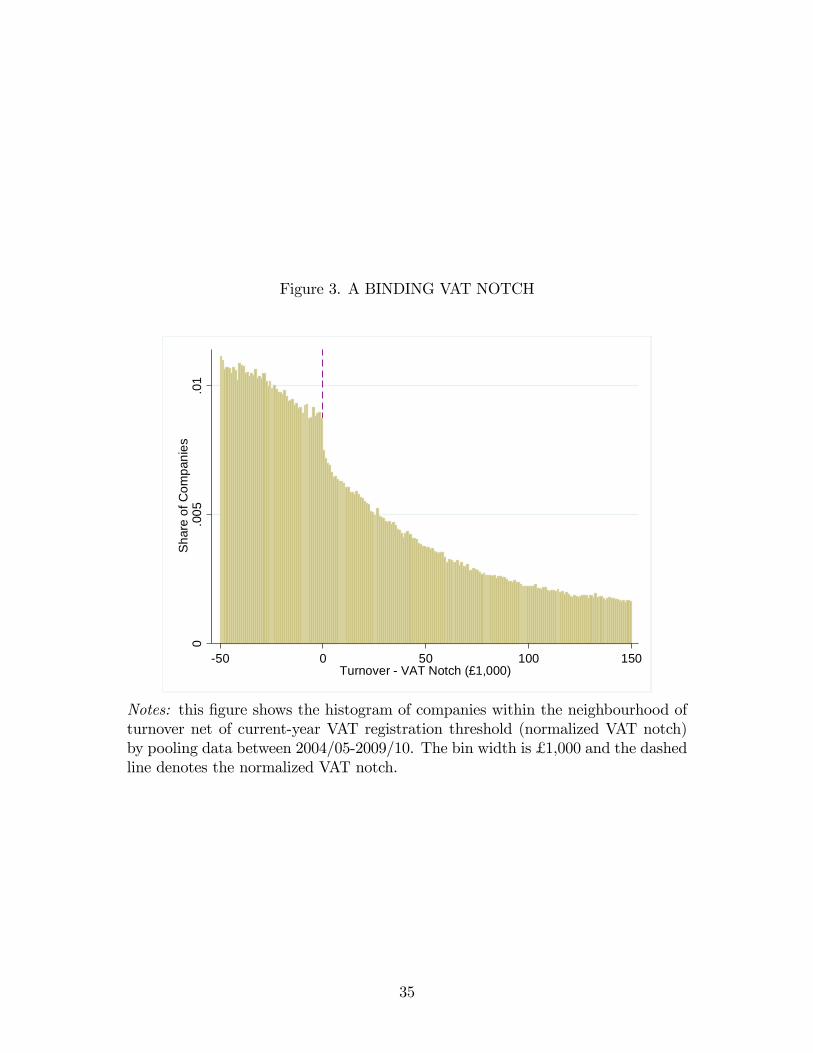
Figure 3. A BINDING VAT NOTCH

0.0

05.0

1S

hare

 of C

ompa

nies

­50 0 50 100 150Turnover ­ VAT Notch (£1,000)

Notes: this figure shows the histogram of companies within the neighbourhood ofturnover net of current-year VAT registration threshold (normalized VAT notch)by pooling data between 2004/05-2009/10. The bin width is £ 1,000 and the dashedline denotes the normalized VAT notch.

35

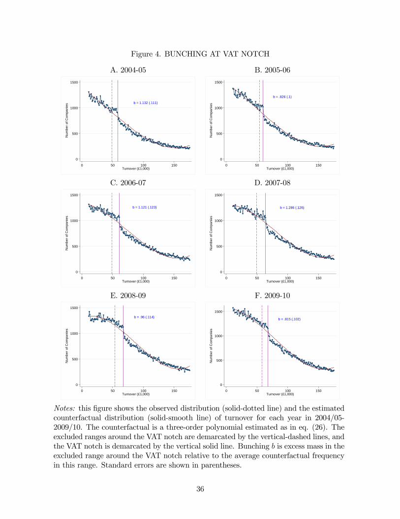
Figure 4. BUNCHING AT VAT NOTCH

A. 2004-05 B. 2005-06

b = 1.132 (.111)

0

500

1000

1500

Num

ber o

f Com

pani

es

0 50 100 150Turnover (£1,000)

b = .826 (.1)

0

500

1000

1500

Num

ber o

f Com

pani

es

0 50 100 150Turnover (£1,000)

C. 2006-07 D. 2007-08

b = 1.121 (.123)

0

500

1000

1500

Num

ber o

f Com

pani

es

0 50 100 150Turnover (£1,000)

b = 1.286 (.126)

0

500

1000

1500

Num

ber o

f Com

pani

es

0 50 100 150Turnover (£1,000)

E. 2008-09 F. 2009-10

b = .96 (.114)

0

500

1000

1500

Num

ber o

f Com

pani

es

0 50 100 150Turnover (£1,000)

b = .815 (.102)

0

500

1000

1500

Num

ber o

f Com

pani

es

0 50 100 150Turnover (£1,000)

Notes: this figure shows the observed distribution (solid-dotted line) and the estimatedcounterfactual distribution (solid-smooth line) of turnover for each year in 2004/05-2009/10. The counterfactual is a three-order polynomial estimated as in eq. (26). Theexcluded ranges around the VAT notch are demarcated by the vertical-dashed lines, andthe VAT notch is demarcated by the vertical solid line. Bunching b is excess mass in theexcluded range around the VAT notch relative to the average counterfactual frequencyin this range. Standard errors are shown in parentheses.

36

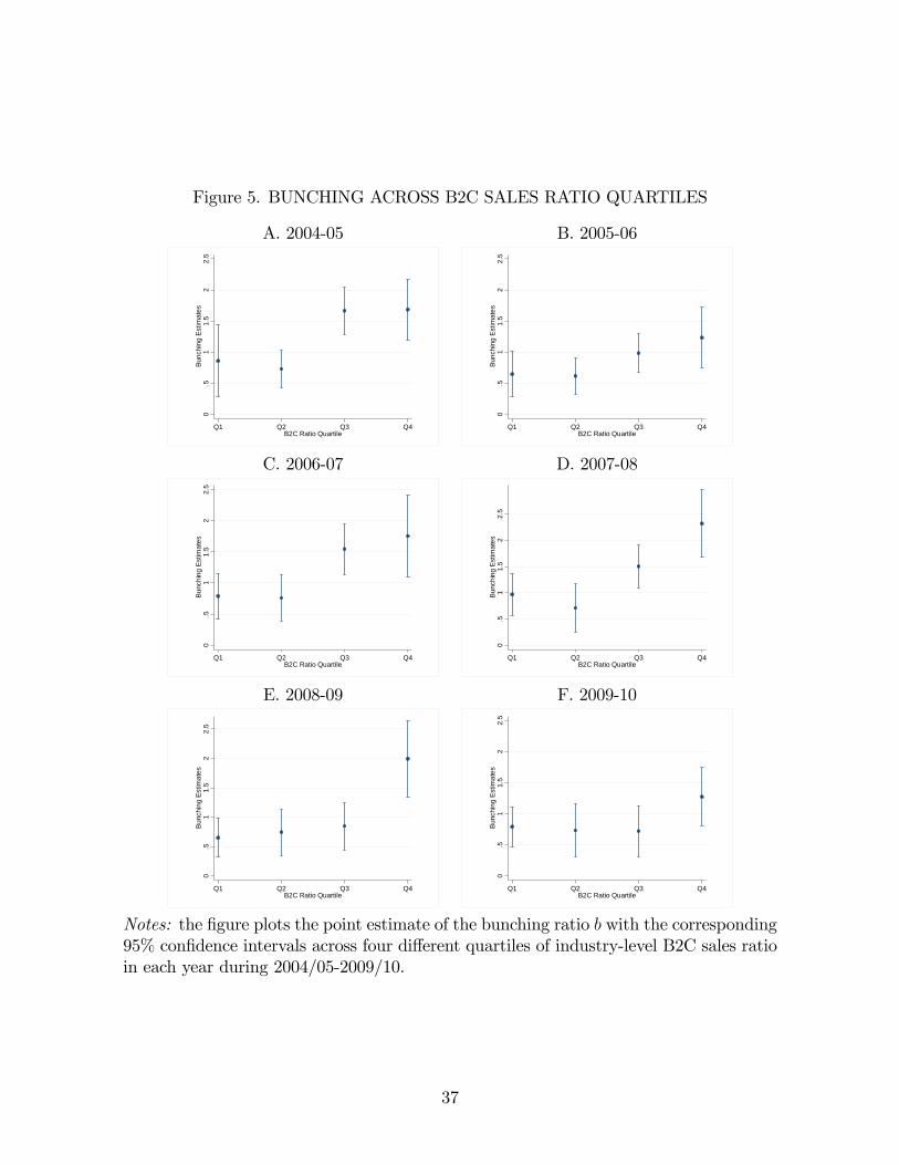
Figure 5. BUNCHING ACROSS B2C SALES RATIO QUARTILES

A. 2004-05 B. 2005-06

0.5

11.

52

2.5

Bun

chin

g Es

timat

es

Q1 Q2 Q3 Q4B2C Ratio Quartile

0.5

11.

52

2.5

Bun

chin

g Es

timat

es

Q1 Q2 Q3 Q4B2C Ratio Quartile

C. 2006-07 D. 2007-08

0.5

11.

52

2.5

Bun

chin

g Es

timat

es

Q1 Q2 Q3 Q4B2C Ratio Quartile

0.5

11.

52

2.5

Bun

chin

g Es

timat

es

Q1 Q2 Q3 Q4B2C Ratio Quartile

E. 2008-09 F. 2009-10

0.5

11.

52

2.5

Bun

chin

g Es

timat

es

Q1 Q2 Q3 Q4B2C Ratio Quartile

0.5

11.

52

2.5

Bun

chin

g Es

timat

es

Q1 Q2 Q3 Q4B2C Ratio Quartile

Notes: the figure plots the point estimate of the bunching ratio b with the corresponding95% confidence intervals across four different quartiles of industry-level B2C sales ratioin each year during 2004/05-2009/10.

37

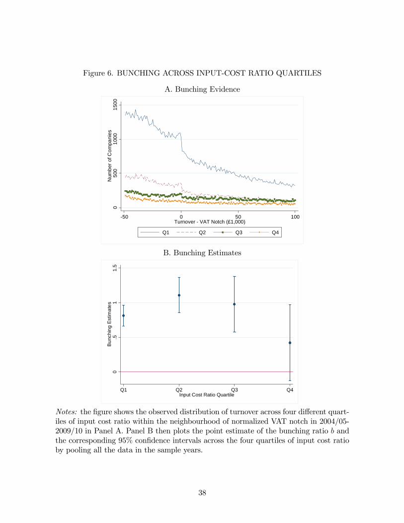
Figure 6. BUNCHING ACROSS INPUT-COST RATIO QUARTILES

A. Bunching Evidence

050

010

0015

00N

umbe

r of C

ompa

nies

­50 0 50 100Turnover ­ VAT Notch (£1,000)

Q1 Q2 Q3 Q4

B. Bunching Estimates

0.5

11.

5B

unch

ing 

Estim

ates

Q1 Q2 Q3 Q4Input Cost Ratio Quartile

Notes: the figure shows the observed distribution of turnover across four different quart-iles of input cost ratio within the neighbourhood of normalized VAT notch in 2004/05-2009/10 in Panel A. Panel B then plots the point estimate of the bunching ratio b andthe corresponding 95% confidence intervals across the four quartiles of input cost ratioby pooling all the data in the sample years.

38

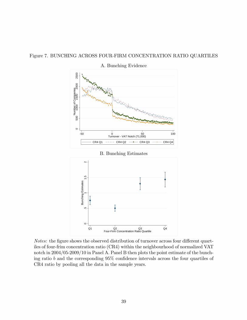
Figure 7. BUNCHING ACROSS FOUR-FIRM CONCENTRATION RATIO QUARTILES

A. Bunching Evidence

050

010

0015

0020

0025

00N

umbe

r of C

ompa

nies

­50 0 50 100Turnover ­ VAT Notch (?1,000)

CR4 Q1 CR4 Q2 CR4 Q3 CR4 Q4

B. Bunching Estimates

0.5

11.

52

Bun

chin

g Es

timat

es

Q1 Q2 Q3 Q4Four­Firm Concentration Ratio Quartile

Notes: the figure shows the observed distribution of turnover across four different quart-iles of four-frim concentration ratio (CR4) within the neighbourhood of normalized VATnotch in 2004/05-2009/10 in Panel A. Panel B then plots the point estimate of the bunch-ing ratio b and the corresponding 95% confidence intervals across the four quartiles ofCR4 ratio by pooling all the data in the sample years.

39

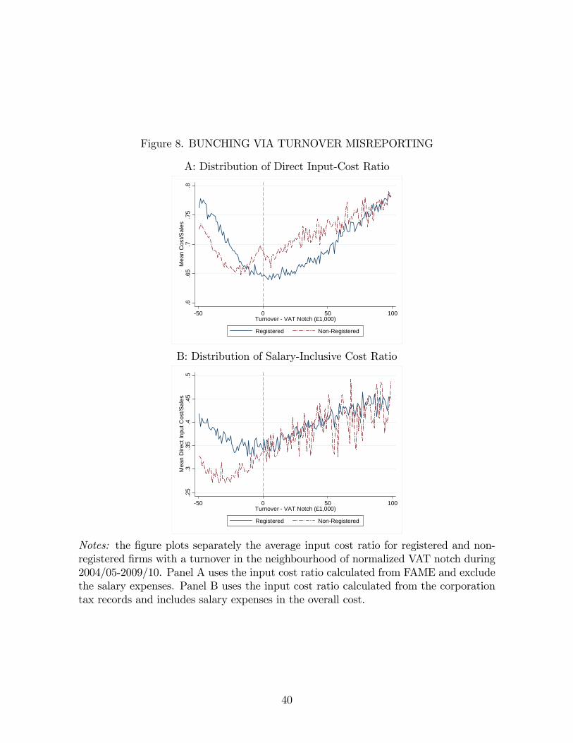
Figure 8. BUNCHING VIA TURNOVER MISREPORTING

A: Distribution of Direct Input-Cost Ratio

.6.6

5.7

.75

.8M

ean 

Cos

t/Sal

es

­50 0 50 100Turnover ­ VAT Notch (£1,000)

Registered Non­Registered

B: Distribution of Salary-Inclusive Cost Ratio

.25

.3.3

5.4

.45

.5M

ean 

Dire

ct In

put C

ost/S

ales

­50 0 50 100Turnover ­ VAT Notch (£1,000)

Registered Non­Registered

Notes: the figure plots separately the average input cost ratio for registered and non-registered firms with a turnover in the neighbourhood of normalized VAT notch during2004/05-2009/10. Panel A uses the input cost ratio calculated from FAME and excludethe salary expenses. Panel B uses the input cost ratio calculated from the corporationtax records and includes salary expenses in the overall cost.

40

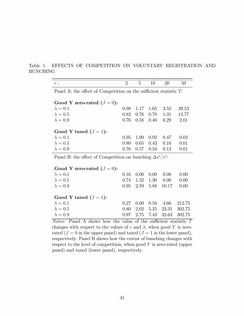
Table 1. EFFECTS OF COMPETITION ON VOLUNTARY REGISTRATION ANDBUNCHING

e : 2 5 10 20 50

Panel A: the effect of Competition on the suffi cient statistic T :

Good Y zero-rated (J = 0):λ = 0.1 0.98 1.17 1.65 3.55 39.53λ = 0.5 0.82 0.76 0.78 1.31 13.77λ = 0.9 0.76 0.58 0.40 0.29 2.01

Good Y taxed (J = 1):λ = 0.1 0.95 1.00 0.92 0.47 0.02λ = 0.5 0.80 0.65 0.43 0.16 0.01λ = 0.9 0.76 0.57 0.34 0.13 0.01

Panel B: the effect of Competition on bunching ∆s∗/s∗:

Good Y zero-rated (J = 0):λ = 0.1 0.16 0.00 0.00 0.00 0.00λ = 0.5 0.74 1.32 1.30 0.00 0.00λ = 0.9 0.95 2.59 5.88 10.17 0.00

Good Y taxed (J = 1):λ = 0.1 0.27 0.00 0.58 4.66 212.75λ = 0.5 0.80 2.02 5.25 23.31 302.75λ = 0.9 0.97 2.75 7.43 32.63 302.75Notes: Panel A shows how the value of the suffi cient statistic Tchanges with respect to the values of e and λ, when good Y is zero-rated (J = 0 in the upper panel) and taxed (J = 1 in the lower panel),respectively. Panel B shows how the extent of bunching changes withrespect to the level of competition, when good Y is zero-rated (upperpanel) and taxed (lower panel), respectively.

41

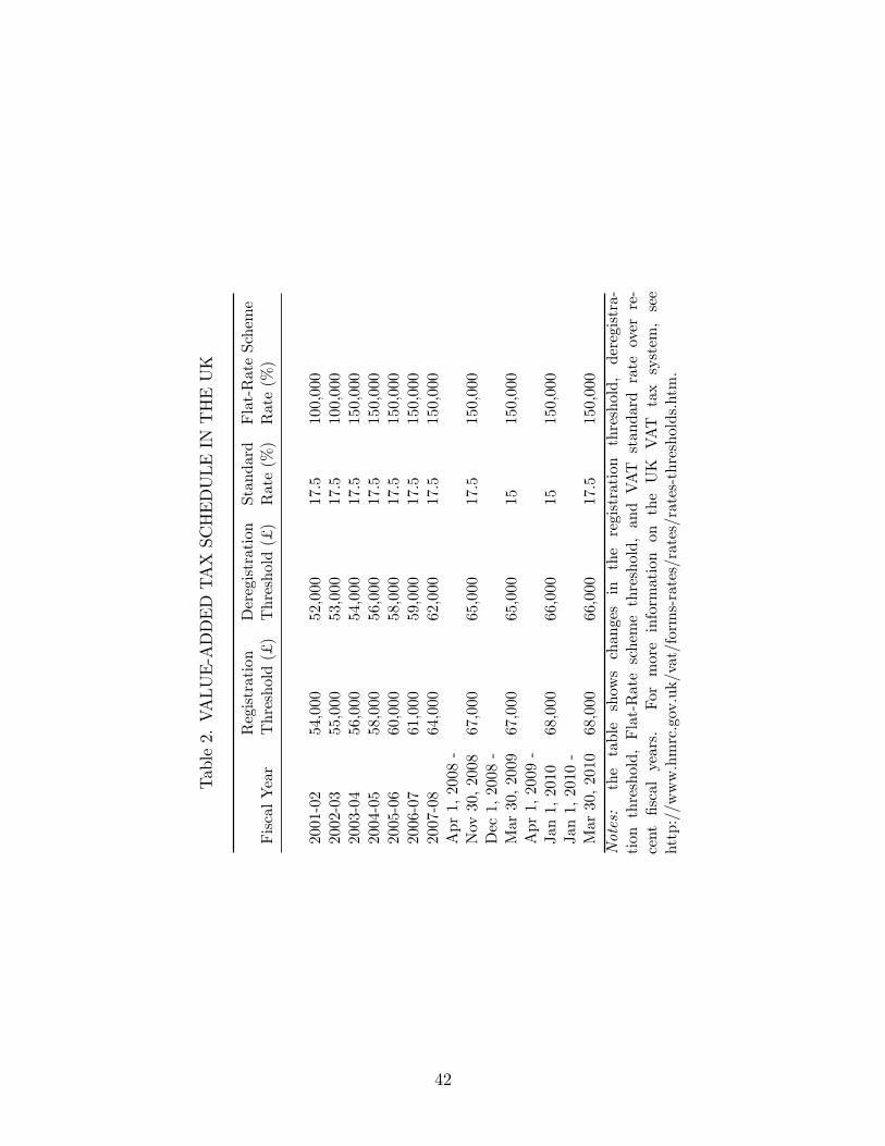
Table2.VALUE-ADDEDTAXSCHEDULEINTHEUK

Registration

Deregistration

Standard

Flat-RateScheme

FiscalYear

Threshold(£)Threshold(£)

Rate(%)Rate(%)

2001-02

54,000

52,000

17.5

100,000

2002-03

55,000

53,000

17.5

100,000

2003-04

56,000

54,000

17.5

150,000

2004-05

58,000

56,000

17.5

150,000

2005-06

60,000

58,000

17.5

150,000

2006-07

61,000

59,000

17.5

150,000

2007-08

64,000

62,000

17.5

150,000

Apr1,2008-

Nov30,2008

67,000

65,000

17.5

150,000

Dec1,2008-

Mar30,2009

67,000

65,000

15150,000

Apr1,2009-

Jan1,2010

68,000

66,000

15150,000

Jan1,2010-

Mar30,2010

68,000

66,000

17.5

150,000

Notes:

thetableshowschangesin

theregistration

threshold,

deregistra-

tion

threshold,Flat-Rateschemethreshold,andVATstandard

rateoverre-

cent

fiscalyears.

Formoreinformationon

theUKVATtaxsystem,see

http://www.hmrc.gov.uk/vat/forms-rates/rates/rates-thresholds.htm.

42

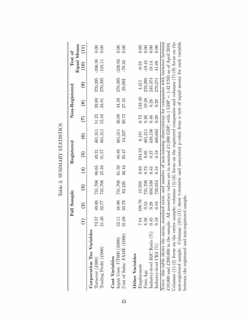
Table3.SUMMARYSTATISTICS

FullSam

ple

Registered

Non-Registered

Testof

EqualMeans

(1)

(2)

(3)

(4)

(5)

(6)

(7)

(8)

(9)

(10)

(11)

CorporationTax

Variables

Turnover(£000)

73.57

49.00

731,706

86.65

49.21

461,311

51.25

39.69

270,395

-336.38

0.00

TradingProfit(£000)

21.46

32.77

731,706

25.16

31.57

461,311

15.16

33.81

270,395

-125.11

0.00

CostVariables

InputCost:CT600(£000)

52.11

48.90

731,706

61.50

48.88

461,311

36.09

44.59

270,395

-226.92

0.00

CostofSales:FAME(£000)

31.08

33.79

82,420

36.44

35.47

54,327

20.72

27.45

28,093

-70.32

0.00

OtherVariables

Employment

7.84

198.76

10,592

8.63

234.53

6,181

6.73

133.40

4,411

-0.53

0.60

FirmAge

8.56

9.53

731,706

8.73

9.05

461,311

8.26

10.28

270,395

-19.45

0.00

Industry-levelB2C

Ratio(%)

0.45

0.28

694,530

0.44

0.27

449,156

0.46

0.28

245,374

18.14

0.00

Industry-levelCR4(%)

0.19

0.19

730,953

0.18

0.18

460,682

0.20

0.20

270,271

41.89

0.00

Notes:thistableshowsthemean,standarderror,andnumberofnon-missingobservationsforcompanieswithturnoverbetween

£10,000and£200,000inthesample.Allmonetaryvaluesareinnominal£1,000GBP,with1GBP=1.42USD

asofApril2016.

Columns(1)-(3)focusontheentiresample;columns(4)-(6)focusontheregisteredcompaniesandcolumns(7)-(9)focusonthe

non-registeredsample.Columns(10)-(11)show

t-statisticandassociatedp-valuefrom

atestofequalmeansforeachvariable

betweentheregisteredandnon-registeredsample.

43

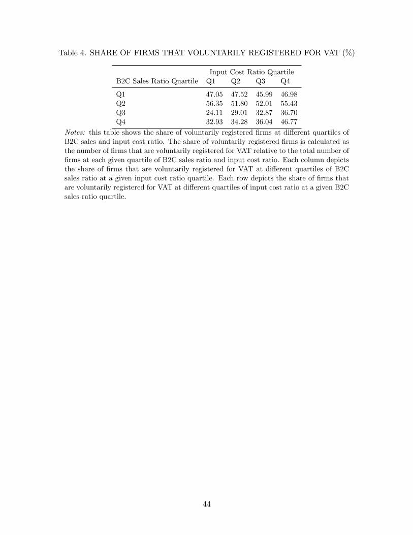
Table 4. SHARE OF FIRMS THAT VOLUNTARILY REGISTERED FOR VAT (%)

Input Cost Ratio QuartileB2C Sales Ratio Quartile Q1 Q2 Q3 Q4

Q1 47.05 47.52 45.99 46.98Q2 56.35 51.80 52.01 55.43Q3 24.11 29.01 32.87 36.70Q4 32.93 34.28 36.04 46.77

Notes: this table shows the share of voluntarily registered firms at different quartiles ofB2C sales and input cost ratio. The share of voluntarily registered firms is calculated asthe number of firms that are voluntarily registered for VAT relative to the total number offirms at each given quartile of B2C sales ratio and input cost ratio. Each column depictsthe share of firms that are voluntarily registered for VAT at different quartiles of B2Csales ratio at a given input cost ratio quartile. Each row depicts the share of firms thatare voluntarily registered for VAT at different quartiles of input cost ratio at a given B2Csales ratio quartile.

44

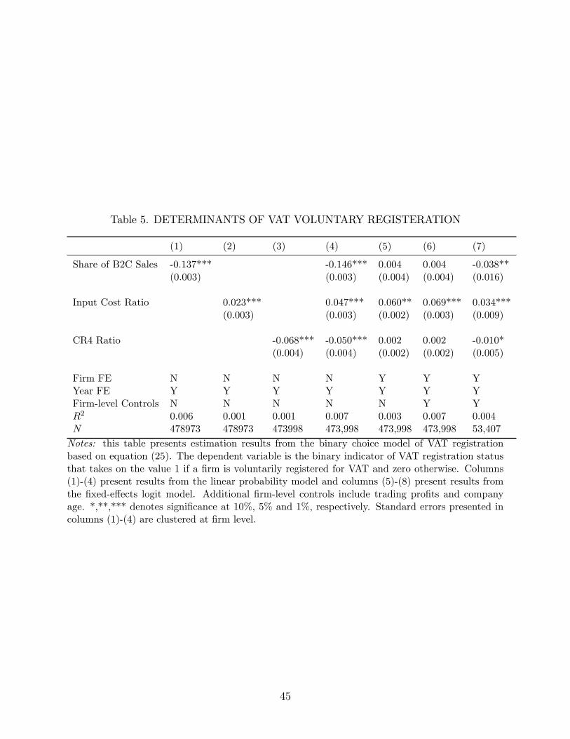
Table 5. DETERMINANTS OF VAT VOLUNTARY REGISTERATION

(1) (2) (3) (4) (5) (6) (7)

Share of B2C Sales -0.137*** -0.146*** 0.004 0.004 -0.038**(0.003) (0.003) (0.004) (0.004) (0.016)

Input Cost Ratio 0.023*** 0.047*** 0.060** 0.069*** 0.034***(0.003) (0.003) (0.002) (0.003) (0.009)

CR4 Ratio -0.068*** -0.050*** 0.002 0.002 -0.010*(0.004) (0.004) (0.002) (0.002) (0.005)

Firm FE N N N N Y Y YYear FE Y Y Y Y Y Y YFirm-level Controls N N N N N Y YR2 0.006 0.001 0.001 0.007 0.003 0.007 0.004N 478973 478973 473998 473,998 473,998 473,998 53,407

Notes: this table presents estimation results from the binary choice model of VAT registrationbased on equation (25). The dependent variable is the binary indicator of VAT registration statusthat takes on the value 1 if a firm is voluntarily registered for VAT and zero otherwise. Columns(1)-(4) present results from the linear probability model and columns (5)-(8) present results fromthe fixed-effects logit model. Additional firm-level controls include trading profits and companyage. *,**,*** denotes significance at 10%, 5% and 1%, respectively. Standard errors presented incolumns (1)-(4) are clustered at firm level.

45

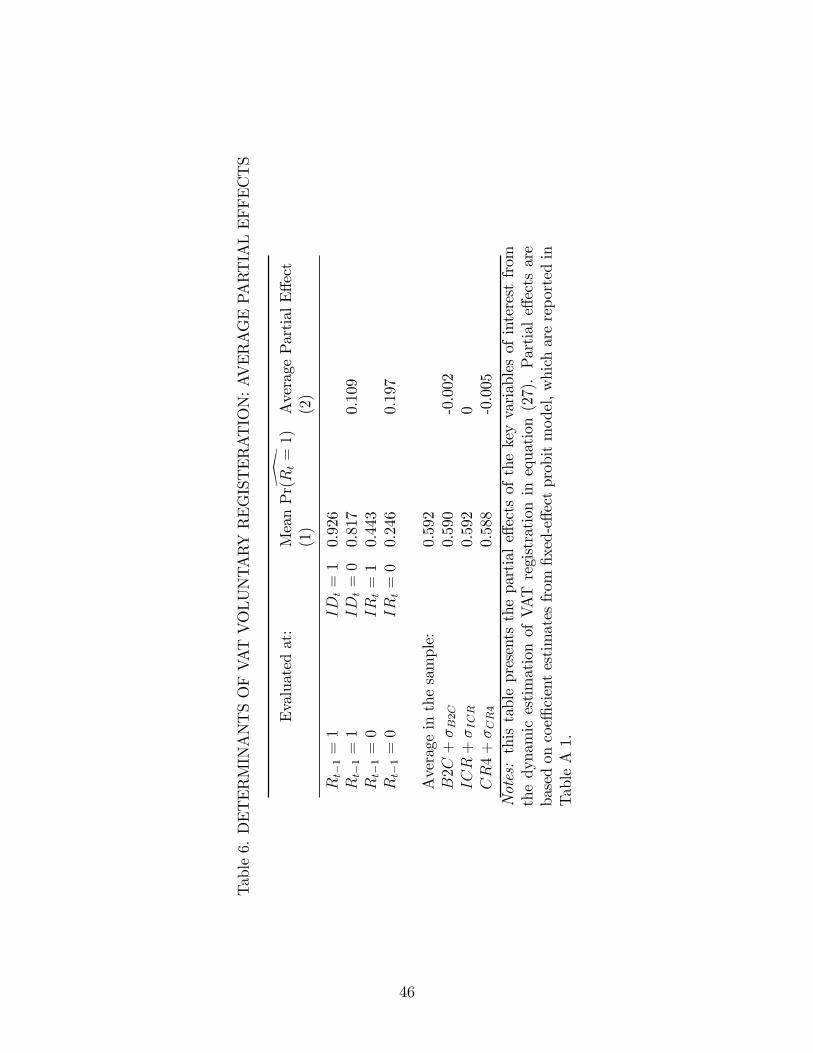
Table6.DETERMINANTSOFVATVOLUNTARYREGISTERATION:AVERAGEPARTIALEFFECTS

Evaluatedat:

Mean

P

r(Rt

=1)

AveragePartialEffect

(1)

(2)

Rt−

1=

1IDt

=10.926

Rt−

1=

1IDt

=00.817

0.109

Rt−

1=

0IRt

=1

0.443

Rt−

1=

0IRt

=0

0.246

0.197

Averageinthesample:

0.592

B2C

+σB

2C

0.590

-0.002

ICR

+σICR

0.592

0CR

4+σCR

40.588

-0.005

Notes:thistablepresentsthepartialeffectsofthekeyvariablesofinterestfrom

thedynamicestimationofVATregistrationinequation(27).Partialeffectsare

basedoncoefficientestimatesfrom

fixed-effectprobitmodel,whicharereportedin

TableA1.

46

A Appendix

Proof of Proposition 1. First, assume only B2C sales i.e. λ = 1. in this case, the firmchooses pC , pB to maximize (10) subject to (11),(12). This is easily solved to give price asa mark-up over cost i.e. pC = eC

eC−1c(I; a) and thus profit for non-registered and registered

firms respectively is

π(0; a) = BC(c(0, a))1−eC , π(1; a) = BC(c(1, a))1−eC 1

(1 + t)eC(A.1)

where BC = AC

(eC−1eC

)eC1

eC−1. So, we only need show that π(0; a) > π(1; a). But, from

(A.1), (8), this holds iff(c(0, a)

c(1, a)

)1−eC

=(ω(1 + t)1−σ + (1− ω)

)(1−eC)/(1−σ)>

1

(1 + t)eC

Now note that as eC > 1,(ω(1 + t)1−σ + (1− ω)

)(1−eC)/(1−σ) ≥ (1 + t)1−eC > (1 + t)−eC

as required.Next, assume only B2B sales i.e. λ = 0. Then, it is easily checked profit is (p −

c(I; a))ABp−eB . So, here, the argument is even simpler; cost is decreasing, and therefore

profit is increasing, if I = 1. �

Proof of Proposition 2. (a) If registered, the firm chooses pC , pB to maximize (10) subjectto (11),(12) when I = 1. This is easily solved to give prices as a mark-up over cost i.e.pC = eC

eC−1c(I; a), pB(a) = eB

eB−1c(I; a), and consequently, maximized profit of

π(1; a) = (λBC(1 + t)−eCc(1; a)1−eC + (1− λ)BBc(1; a)1−eB) (A.2)

where as before, BC = AC

(eC−1eC

)eC1

eC−1, and also BB = AB

(eB−1eB

)eB1

eB−1.

Next, if not registered, the firm chooses pC , pB to maximize (10) subject to (11),(12) whenI = 0, subject also to the constraint pCx + pBy ≤ s∗ that the total value of sales is belowthe threshold. Now consider voluntary registration. A necessary and suffi cient condition forthis is that profit with registration is greater than profit without, ignoring the constraintthat sales be below the threshold. We will assume that a firm will register if indifferent, tobreak the tie. Following the case for the registered firm, we can show that the profit of anunregistered firm, ignoring the constraint that sales be below the threshold is

π(0; a) = (λBCc(0; a)1−eC + (1− λ)BBc(0; a)1−eB) (A.3)

Then, the voluntary registration condition is π(1; a) ≥ π(0; a). After some simple rearrange-ment, using (A.2),(A.3), this reduces to (16).(b) We only need show that the RHS of (16) is increasing in λ and decreasing in ω. The

47

statement for λ is obvious by inspection. For ω, note first that 1+∆c ≡ (ω(1 + t)1−σ + 1− ω)1/(1−σ)

is increasing in ω. So, both (1 + ∆c)1−eC , (1 + ∆c)

1−eB are decreasing in ω as eC , eB >1. Finally, note that as ∆c > 0, eB > 1, 1 − (1 + ∆c)

1−eB > 0. So, the RHS of (16) T isdecreasing in ω as required.(b) If eB = eC = e, and using AC = 1, (16) rearranges to

λ(1 + t)−e + (1− λ)ABλ+ (1− λ)AB

(1 + ∆d)e−1 > 1 (A.4)

But thenλ(1 + t)−e + (1− λ)AB

λ+ (1− λ)AB= 1− λ(1− (1 + t)−e)

λ+ (1− λ)AB= 1−∆d (A.5)

Combining (A.4),(A.5) gives (17).(c) Note that lime→∞

(1− 1

e

)e= 1/ exp ' 0.37, and ∆c > 0, so if J = 0, it is clear that

as e→∞, the LHS of (A.4) tends to infinity, so it always holds for e high enough. On theother hand, if J = 1, (A.4) becomes

λ+ (1− λ)(e−1e

)eλ(1 + t)e + (1− λ)

(e−1e

)e (1 + ∆c)e−1 > 1

which behaves for e large, like(

(ω(1+t)1−σ+1−ω)1/(1−σ)

1+t

)e. But the number in the bracket is

strictly less than 1 + t, independently of e, so in this case, T → 0 as e→∞. �

Proof of Proposition 3. The indifference condition that determines a∗ + ∆a∗ is (20). Touse this condition, we proceed as follows. To lighten notation, and using eC = eB = e, define

A0 = λ+ (1− λ)AB, A1 = λ(1 + t)−e + (1− λ)AB

First, from (A.2), and using the restriction that eC = eB = e, a firm that registers hasmaximized profit:

π(1; a) = A1

(e

1− e

)−eae−1

1− e (A.6)

Next, the profit from being just at the VAT threshold for an a−type when constrained is

π(0; a) = s∗ − 1 + ∆c

a

s∗

p(A.7)

But solving for p from the constraint A0p1−e = s∗, we get p =

(s∗

A0

)−1/(e−1)

. Substituting

this back into (A.7), and using a = a∗ + ∆a∗, we get

π(0; a∗ + ∆a∗) = s∗ − 1 + ∆c

A1/(e−1)0 (a∗ + ∆a∗)

(s∗)e/(e−1) (A.8)

48

Also combining (21) and (A.8), we get:

π(0; a∗ + ∆a∗) = s∗ − 1 + ∆c

A1/(e−1)0 (a∗ + ∆a∗)

(s∗)e/(e−1) (A.9)

= s∗ − (s∗)e/(e−1)

(e− 1

e

)(s∗ + ∆s∗)1/(1−e)

Now using (21) in (A.6), we get:

π(1; a∗ + ∆a∗) = A1

(e

1− e

)−e1

1− e(a∗ + ∆a∗)e−1 (A.10)

=A1

A0

(e

1− e

)−e1

1− e

(e (1 + ∆c)

e− 1

)e−1

(s∗ + ∆s∗)

=T

e(s∗ + ∆s∗)

So, using (A.10),(A.9), the indifference condition π(1; a∗ + ∆a∗) = π0(0; a∗ + ∆a∗) becomes

s∗ − (s∗)e/(e−1)

(e− 1

e

)(s∗ + ∆s∗)1/(1−e) − T

e(s∗ + ∆s∗) = 0 (A.11)

After some simplification of (A.11) (divide through by s∗, then 1 + ∆s∗

s∗ , and multiply by e)we get (22) as required. �

Proof of Proposition 4. First, (22) can be rewritten as

f(x, e)− T (λ, ω, e)= 0, f(x) ≡ ex− (e− 1)xe/(e−1), x =1

(1 + ∆s∗/s∗)(A.12)

So, from (A.12):dx

dλ=Tλfx,dx

dω=Tωfx,dx

de=Te − fefx

(A.13)

Moreover, note thatfx = e(1− x1/(e−1)) > 0 (A.14)

because x < 1, and e > 1, so x1/(e−1) < 1. Also, we know that Tλ < 0, Tω > 0 and so from(A.13), (A.14), we conclude that dx

dλ< 0, dx

dω> 0. As x is an inverse measure of bunching, it

follows that as λ increases, ∆s∗ rises, and ω rises, ∆s∗ falls. �The Value-Added of A Registered Small Firm. If σ = 0, a firm uses ω

aunits of the

input per unit of output. So, the value added of a registered "small" firm is the value ofoutput minus the value of inputs used i.e.;

V A = pCx+ pBy −ω

a(x+ y)

Now assuming A1 and eC = eB, and the mark-up expressions for prices, i.e. pC = pB = p =

49

ee−1

1a, the firm’s value-added is

V A =1

a

(e

e− 1− ω

)(x+ y)

∝ λ(1 + t)−e + (1− λ)

(e− 1

e

)e(1 + J.t)−e

So, if J = 1, the elasticity of V A with respect to 1 + t is e, as claimed.Calibration of ω. The average share of costs that is non-labour is

ICR =ω(1 + φt)

ω(1 + φt) + 1− ω

where φ the fraction of overall sales that are by registered firms. Now φ = 0.74, andICR = 0.496, and t = 0.175, so

0.496 =1.123ω

1.123ω + 1− ω

which implies ω = 0.419.

50

B Not-For-Publication Appendix

General Proof that Voluntary Registration is not Possible with Only B2C Sales.Consider a firm facing a residual demand function from final consumers of x(q), where q isthe consumer price. This covers both the cases of monopoly, where x(.) is also the actualdemand curve, and monopolistic competition, where x(.) is demand for that firm’s product,taking the prices of all other firms as fixed. Assume all sales are to final consumers i.e. B2C.If a firm is registered for VAT, profit is then

πR(p) = px(p(1 + t))− c(x(p(1 + t)), w, r)

where p is the producer price, and c(x, w, r) is the cost function given output x, and pricesof labour and the intermediate input w, r. This is completely general cost function thatincludes the constant returns CES cost function in the paper as a special case. If the firm isnot registered for VAT, profit is

πN(p) = px(p)− c(x(p), w, r(1 + t))

Then, we have

πR = maxp{px(p(1 + t))− c(x(p(1 + t)), w, r)}

= maxq

{q

1 + tx(q)− c(x(q), w, r)

}=

1

1 + tmaxq{qx(q)− (1 + t) c(x(q), w, r)}

< maxq{(q − c(x(q), w, r(1 + t)))}

= πN

So, with only B2C sales, no firm would every wish to register voluntarily.The Competitive Economy. here, we present a competitive variant of the model and show(i) that without segmented markets i.e. different markets for B2B and B2C transactions,the equilibrium is trivial, with all firms registering for VAT; (ii) with segmented markets,there is generically complete sorting, with registered (non-registered) firms only selling B2B(resp. B2C). Moreover, in the second case, the equilibrium actually has a more complexstructure,being defined by three equations, than in the monopolistic case, which makesgenerating empirical predictions more diffi cult.Consider a "competitive" version of the model in the paper, where the small firms sell

a homogenous product, with the model unchanged in all other respects. In particular, thesmall firms face fixed prices pB, pC in the B2B and B2C markets respectively. Moreover, B2Band B2C demand for the product of the small firms is now given by the perfect competition

analogues of (4) and (l3) i.e. λ (pC)−φ , (1 − λ)(

γ1−γ

)−γ(pB)−γ . So, the revenue per unit

sold by registered and non-registered firms is as in the Table below:

Table B1: Revenue Per Unit

1

registered firms non-registered firms

B2C pC1+t

pC

B2B pB pB

This is because a registered firm perceives perfectly elastic demand at consumer pricepC in the B2C market, and so must bear all the burden of output VAT. The next stepsto specify firms’cost and profit. With perfect competition, firm’s cost function need to bestrictly convex in order for firm scale to be well-defined. Without much loss of generality, andfor easy comparison to the main model in the paper, we assume that the firm productionfunctions are CES and homogeneous of degree 1/δ, δ > 1, so the firm’ cost function isc(I(a); a)yδ, where c(I(a); a) is defined in (8).Consider first the case where markets are not segmented; then arbitrage by buyers implies

pC = pB = p. But then if a firm registers, by Table A1, it will prefer to sell B2B, and canthus get maximum profit

πR(a) = maxy

{py − c(1; a)yδ

}If a firm does not register, it is indifferent to whom it sells, and makes profit

πN(a) = maxy

{py − c(0; a)yδ s.t. py ≤ s∗

}where as in the main paper, s∗ is the VAT threshold. So, clearly, as c(0; a) > c(1; a), allfirms will wish to register, as claimed. [It is not clear that this is an equilibrium, however,as final consumers will receive no supply, and they are willing to pay for supply].If markets are segmented, then (ignoring non-generic cases) for an equilibrium to exist,

by the above table the two prices must satisfy:

pC1 + t

< pB < pC (B.1)

For any other price configuration, both types of firms would not wish to supply eitherfinal consumers or businesses, and that could not be an equilibrium, because from iso-elasticdemand, the buyer without supply would be willing to pay an arbitrarily high price for thegood. Note that for this price configuration, there is complete sorting i.e.registered firmsonly sell B2B, and non-registered firms only sell B2C41.

But then, using (B.1), the profits to registering and not are

πR(a) = maxy

{pBy − c(1; a)yδ

}, πN(a) = max

y

{pCy − c(0; a)yδ s.t. pCy ≤ s∗

}If firms differ in the input cost ratio, there may be both voluntary registration and bunching,as in the main model. To see this, first note that a firm of type a will register voluntarily

41In can be shown that in the model of the main paper, there is partial sorting i.e. registered firms sellrelatively more B2B than non-registered firms do, and that if eC = eB = e, this sorting effect is stronger, thehigher is e i.e. the more competitive is the market for the differentiated good. Moreover, in the competitivelimit as e→∞, there is complete sorting. A proof of this available on request.

2

iff πR(a) is greater than the payoff from not registering, ignoring the constraint pCy ≤ s∗.After performing the maximisations, the condition reduces to

(pB)δ/(δ−1)(c(1; a))−1/(δ−1) ≥ (pC)δ/(δ−1)(c(0; a))−1/(δ−1)

and finally to a condition independent of a;

pBpC≥(c(1; a)

c(0; a)

)1/δ

(B.2)

This condition says that voluntary registration will occur for those firms where the loss ofrevenue from a lower price, measured inversely by pB/pC , is less than the cost gain frombeing registered, measured inversely by c(1; a)/c(0; a). On the face it it, this is a simplercondition than (17) in the paper. In particular, it is clear that conditional on pB

pC, the higher

the input cost ratio, the more likely this is to be satisfied. However, recall that pB, pC areendogenous and remain to be determined.Assume now that there are some firms with an input -cost ratio such that (B.2) is not

satisfied. Then, by an argument as in the main paper, some of these firms will bunch i.e.there will be a critical a such that πR(a) = πN(a), so that only firms above a will register. Thiscan be manipulated into a condition similar to (22). Finally, the two prices are determinedin equilibrium by the two conditions

λ (pC)−φ =

a∫a

yN(pC ; a)da, (1− λ)

(γ

1− γ

)−γ((1 + Jt)pB)−γ =

a∫a

yR(pB; a)da (B.3)

where the supply functions are defined as;

yR(pB; a) = arg maxy

{pBy − c(1; a)yδ

}yN(pC ; a) = arg max

y

{pCy − c(0; a)yδ s.t. pCy ≤ s∗

}So, in equilibrium, a and the prices (pB, pC) are determined by three simultaneous conditionsπR(a) = πN(a), and (B.3). The effects of changes in ω and λ on voluntary registration andbunching could no doubt be calculated, but this may be a complex exercise.Derivation of the Bunching Equation with Evasion. The proof follows the proof ofProposition 4 in the paper, with the following changes. First, we define A0, A1 as

A0 = λ(1− ν) + (1− λ)AB, A1 = (λ(1 + (1− ν)t)−e + (1− λ)AB)

As in (A.2) in the paper, any firm that registers has maximized profit:

π(1; a) = A1

(e

1− e

)−eae−1

1− e (B.4)

3

Next, the payoff from being on the VAT threshold for an a−type when constrained is now

π(0; a) = (s∗ + νpx)− 1 + ∆c

a

(s∗ + νpx)

p(B.5)

This is because the firm can actually produce and sell s∗ + νpx with a threshold s∗ becausesales νpx are "cash" and thus not observable by the tax authority. Solving for p from thedefinition that non-concealed sales must be equal to s∗ i.e. ((1− ν)λ+ (1− λ)AB)p1−e = s∗,we get:

p =

(s∗

(1− ν)λ+ (1− λ)AB

)−1/(e−1)

Combining this with the fact that x = λp1−e, we get

s∗ + νpx = s∗λ+ (1− λ)AB

(1− ν)λ+ (1− λ)AB≡ µs∗

Substituting this back into (B.5), and setting a = a∗ + ∆a∗, we get

π(0; a∗ + ∆a∗) = µ

(s∗ − 1 + ∆c

A1/(e−1)0 (a∗ + ∆a∗)

(s∗)e/(e−1)

)(B.6)

Also observed non-cash sales map into type by

s∗ + ∆s∗ = A0

(e (1 + ∆c)

e− 1

)1−e

(a∗ + ∆a∗)e−1, A0 = λ(1− ν) + (1− λ)AB (B.7)

Combining (B.7) and (B.6), we get:

π(0; a∗ + ∆a∗) = µ

(s∗ − 1 + ∆c

A1/(e−1)0 (a∗ + ∆a∗)

(s∗)e/(e−1)

)(B.8)

= µ

(s∗ − (1 + ∆c) (s∗)e/(e−1)

A1/(e−1)0

(A0)1/(e−1)

(e− 1

ec0

)(s∗ + ∆s∗)1/(1−e)

)

= µ

(s∗ − (s∗)e/(e−1)

(e− 1

e

)(s∗ + ∆s∗)1/(1−e)

)

4

Now using (B.7) in (B.4), we get:

π(1; a∗ + ∆a∗) = A1

(e

1− e

)−e1

1− e(a∗ + ∆a∗)e−1 (B.9)

=A1

A0

(e

1− e

)−e1

1− e

(ec0

e− 1

)e−1

(s∗ + ∆s∗)

=A1(1 + ∆c)

e−1

eA0

(s∗ + ∆s∗)

= T (ν)s∗ + ∆s∗

e

So, using (B.8),(B.9), the indifference condition π(1; a∗ + ∆a∗) = π0(0; a∗ + ∆a∗) becomes

s∗ − (s∗)e/(e−1)

(e− 1

e

)(s∗ + ∆s∗)1/(1−e) − T (ν)

µe(s∗ + ∆s∗) = 0 (B.10)

After some simplification of (B.10) (divide through by s∗, then 1 + ∆s∗

s∗ , and multiply by e)we get (22) in the paper with the tax term T (ν)

µ= T (ν) λ+(1−λ)AB

(1−ν)λ+(1−λ)ABas required. �

C Supplementary Tables

5

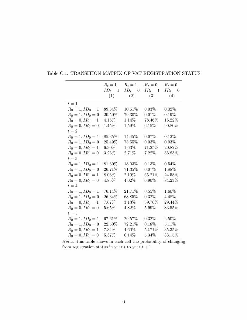
Table C.1. TRANSITION MATRIX OF VAT REGISTRATION STATUS

Rt = 1 Rt = 1 Rt = 0 Rt = 0IDt = 1 IDt = 0 IRt = 1 IRt = 0(1) (2) (3) (4)

t = 1R0 = 1, ID0 = 1 89.34% 10.61% 0.03% 0.02%R0 = 1, ID0 = 0 20.50% 79.30% 0.01% 0.19%R0 = 0, IR0 = 1 4.18% 1.14% 78.46% 16.22%R0 = 0, IR0 = 0 1.45% 1.59% 6.15% 90.80%t = 2R0 = 1, ID0 = 1 85.35% 14.45% 0.07% 0.12%R0 = 1, ID0 = 0 25.49% 73.55% 0.03% 0.93%R0 = 0, IR0 = 1 6.30% 1.63% 71.25% 20.82%R0 = 0, IR0 = 0 3.23% 2.71% 7.22% 86.83%t = 3R0 = 1, ID0 = 1 81.30% 18.03% 0.13% 0.54%R0 = 1, ID0 = 0 26.71% 71.35% 0.07% 1.88%R0 = 0, IR0 = 1 8.03% 2.19% 65.21% 24.58%R0 = 0, IR0 = 0 4.85% 4.02% 6.90% 84.23%t = 4R0 = 1, ID0 = 1 76.14% 21.71% 0.55% 1.60%R0 = 1, ID0 = 0 26.34% 68.85% 0.32% 4.48%R0 = 0, IR0 = 1 7.67% 3.13% 59.76% 29.44%R0 = 0, IR0 = 0 5.65% 4.82% 5.99% 83.55%t = 5R0 = 1, ID0 = 1 67.61% 29.57% 0.32% 2.50%R0 = 1, ID0 = 0 22.50% 72.21% 0.18% 5.11%R0 = 0, IR0 = 1 7.34% 4.60% 52.71% 35.35%R0 = 0, IR0 = 0 5.37% 6.14% 5.34% 83.15%

Notes: this table shows in each cell the probability of changingfrom registration status in year t to year t+ 1.

6

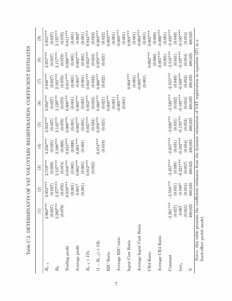
TableC.2.DETERMINANTSOFVATVOLUNTARYREGISTERATION:COEFFICIENTESTIMATES

(1)

(2)

(3)

(4)

(5)

(6)

(7)

(8)

(9)

Rt−

12.963***

2.952***

2.719***

3.256***

2.953***

2.958***

2.948***

2.957***

2.955***

(0.027)

(0.027)

(0.029)

(0.025)

(0.027)

(0.027)

(0.027)

(0.027)

(0.027)

R0

2.282***

2.277***

2.127***

2.100***

2.142***

2.120***

2.161***

2.117***

2.125***

(0.079)

(0.076)

(0.074)

(0.069)

(0.070)

(0.070)

(0.070)

(0.070)

(0.070)

Tradingprofit

0.019***

0.016***

0.012***

0.008***

0.008***

0.011***

0.008***

0.011***

(0.001)

(0.001)

(0.000)

(0.001)

(0.001)

(0.001)

(0.001)

(0.001)

Averageprofit

0.001*

0.002***

0.001***

0.002***

0.002***

-0.001*

0.002***

-0.002*

(0.001)

(0.001)

(0.001)

(0.001)

(0.001)

(0.001)

(0.001)

(0.001)

Rt−

1×IDt

0.812***

0.937***

0.953***

0.941***

0.933***

0.944***

(0.022)

(0.024)

(0.024)

(0.024)

(0.024)

(0.024)

(1−Rt−

1)×IRt

0.874***

0.976***

0.988***

0.980***

0.979***

0.983***

(0.019)

(0.021)

(0.021)

(0.022)

(0.021)

(0.022)

B2C

Ratio

0.003***

0.003***

(0.001)

(0.001)

AverageB2C

ratio

-0.005***

-0.005***

(0.001)

(0.001)

InputCostRatio

0.004***

0.004***

(0.001)

(0.001)

AverageInputCostRatio

-0.005***

-0.004***

(0.001)

(0.001)

CR4Ratio

0.002***

0.002***

(0.000)

(0.000)

AverageCR4Ratio

-0.007***

-0.006***

(0.001)

(0.001)

Constant

-2.261***

-2.558***

-2.457***

-2.657***

-2.626***

-2.520***

-2.555***

-2.516***

-2.432***

(0.027)

(0.031)

(0.030)

(0.031)

(0.031)

(0.032)

(0.049)

(0.031)

(0.049)

lnσu

-0.067

-0.100*

-0.221***

-0.192***

-0.176***

-0.192***

-0.169***

-0.197***

-0.195***

(0.055)

(0.054)

(0.057)

(0.054)

(0.053)

(0.054)

(0.053)

(0.054)

(0.054)

N480,025

480,025

480,025

480,025

480,025

480,025

480,025

480,025

480,025

Notes:thistablepresentsthecoefficientestimatesfrom

thedynamicestimationofVATregistrationinequation(27)ina

fixed-effectprobitmodel.

7