Evaluating Tax Reforms without Elasticities:

What Bunching Can Identify

Dylan T. Moore∗

[Job Market Paper: Click here for latest version]

January 20, 2022

Abstract

I present a new method for evaluating proposed reforms of progressive piecewise linear tax

schedules. Typically, estimates of the elasticity of taxable income (ETI) are used to predict

taxpayer responses to changes in tax rates and/or tax bracket thresholds. I show that elasticities

are not always needed for this task; the “bunching mass” at a bracket threshold (the share of

taxpayers locating there) is a sufficient statistic for the revenue effect of behavioral responses

to small changes of the threshold. Building on this finding, revenue forecasting and welfare

analysis of threshold changes can be conducted using the pre-reform distribution of taxable

income alone. I apply these results in an analysis of the Earned Income Tax Credit, an exercise

which motivates extensions addressing taxpayer optimization errors, tax rate heterogeneity, large

reforms, and income and participation effects. My approach complements existing bunching

methods: it avoids key limitations of bunching-based ETI estimation, but addresses a relatively

narrower set of policy questions.

∗PhD Candidate. Department of Economics, University of Michigan, Ann Arbor, MI, 48109, United States. Email:dtmoore@umich.edu. I am grateful for helpful comments on earlier drafts received from Ashley C. Craig, James R.Hines Jr., Nirupama Rao, Parker Rogers, Nathan Seegert, Joel Slemrod, Ellen Stuart, and Tejaswi Velayudhan. Ialso thank seminar participants at the University of Michigan as well as conference participants at the Michigan TaxInvitational 2021, the Young Economist Symposium 2021, and the 114th Annual Conference on Taxation for theirvaluable feedback.

1

Progressive, piecewise linear income tax schedules are ubiquitous in modern economies. In such

schedules, the marginal tax rate is constant within brackets but varies across brackets, increasing

discontinuously at thresholds separating the brackets. Major tax reforms in these economies

frequently feature both rate and bracket changes. Consider, for example, the Tax Cuts and Jobs Act

of 2017 (TCJA), which substantially reformed the US income tax schedule. This reform reduced tax

rates across five out of seven brackets of the US federal income tax schedule, and simultaneously

changed the location of many tax bracket thresholds.1 For example, single tax filers in 2017 entered

the top tax bracket when their taxable income surpassed $418,400. The TCJA moved this threshold

to $500,000 in 2018. The TCJA also featured a substantial increase in the standard deduction,

which effectively increased all bracket thresholds as function of pre-deduction income.2

Accurately forecasting the revenue impact and efficiency consequences of a proposed tax reform like

the TCJA requires a prediction of how tax policy changes will alter taxpayer behavior. That is, it

requires estimating the behavioral response to taxation. In modern tax analysis, the elasticity of

taxable income (ETI) is a key measure of behavioral responses.3 Estimates of the ETI are commonly

employed by government agencies tasked with forecasting the fiscal impact of proposed tax reforms.4

However, estimates of the ETI are subject to substantial internal and external validity challenges.

These estimates vary considerably according to the methodological approach adopted (Aronsson,

Jenderny, and Lanot, 2018; Kumar and Liang, 2020; Neisser, 2021; Saez, Slemrod, and Giertz, 2012;

Weber, 2014). Furthermore, there is a strong theoretical and empirical rationale for expecting the

ETI to vary substantially with features of the tax system and other contextual factors (Jacquet and

Lehmann, 2021; Kopczuk, 2005; Neisser, 2021; Slemrod and Kopczuk, 2002).

This paper shows that for some important features of tax policy there may be no need to rely on ETI

estimates in revenue forecasting. I present a new approach to predicting the revenue and welfare

effects of tax reforms that include changes to brackets. The proposed method takes advantage of a

notable feature of taxpayer behavior under a progressive piecewise linear tax schedule: bunching at

kinks. Such schedules induce convex kinks in taxpayer budget sets at bracket thresholds, where the

marginal benefit of earning an additional dollar falls discontinuously. Consequently, for a large mass

of taxpayers it is optimal to “bunch”: to earn precisely the amount of income that lands them at

the kink point (i.e. at the tax bracket threshold).

The central finding of this paper is that the share of taxpayers who are bunching at a given kink

(the “bunching mass”) identifies the revenue impact of taxpayer responses to small changes in the

1In many countries such as the US, tax bracket thresholds change every year in a bid to account for inflation.When I talk about a reform that changes these thresholds, I mean that it substantially altered their location in termsof real income.

2While the tax code defines brackets in terms of taxable income after subtracting various deductions, from aneconomic theory perspective we care about what taxpayer budget constraints look like as a function of total income.

3Feldstein (1999) shows that the ETI can be viewed as a sufficient statistic for the efficiency costs (deadweight loss)of taxation.

4For example, the Canadian Parliamentary Budget Office (PBO) uses estimates of the ETI to as-sess the likely revenue effects of actual and hypothetical tax reforms at the request of Membersof Parliament and political parties during election campaigns. See, for instance, https://www.pbo-dpb.gc.ca/web/default/files/Documents/Reports/2016/PIT/PIT EN.pdf.

2

location of the kink point. This implies that the revenue effect of moving a tax bracket threshold

can be identified from the observed pre-reform distribution of taxable income alone, without relying

on ETI estimates.5 After documenting this result, I explore how it might be used to evaluate actual

and potential reforms of real-world tax schedules. I also discuss the implications of these findings

for the literature on the use of bunching to estimate the ETI.

Section 1 presents the main finding in the case of a simple two-bracket piecewise linear tax schedule.

I assume only that taxpayers have continuous, convex preferences and that they make a frictionless

choice of income, allowing for arbitrary heterogeneity in taxpayer preferences.6 In this setting, the

bunching mass is a sufficient statistic for the first-order revenue effect of the behavioral responses

caused by changing the location of the threshold separating the two brackets. That is, bunching

identifies the behavioral response effect of moving a convex kink point.

The formal derivation of this finding is straightforward, but the intuition behind it is somewhat

subtle. Suppose a kink point (tax bracket threshold) is reduced by a small amount, raising the

marginal tax rate on income in the window between the new kink and the original kink. This

reform raises additional revenue from the taxpayers above the kink who pay a higher tax rate on

their income within this window but whose marginal tax rate is unchanged (the mechanical effect).

However, it also causes some changes in taxpayer behavior that in turn alter tax revenue: the

behavioral response effect of the reform.

Absent income or labor force participation effects, this behavioral response effect has three parts.

Holding constant the size of the bunching mass there is a loss in revenue due to the fact this mass is

moved to a lower level of income at the new kink. However, the bunching mass will not remain

constant. Some individuals are former bunchers : those who bunched at the old kink but will choose

not to bunch at the new kink, instead locating somewhere in the upper tax bracket below the

old kink. Additionally, some individuals are new bunchers: those who used to locate in the lower

bracket at a spot above the new kink will begin bunching at the new kink point.

I show that the revenue impact of the behavioral responses of the new and former bunchers reform are

second-order. This result obtains in spite of the fact that moving a kink point has a first-order effect

on the size of the bunching mass. It is a consequence of the fact that—to a first approximation—the

decisions of taxpayers who are at the margin of entering or leaving the bunching mass cause no

change in tax revenue. Section 1 presents a graphical derivation to build intuition for this result.

Section 2 of the paper explores the implications of this finding for ex ante evaluation of reforms to

progressive, piecewise linear income tax schedules. First, I discuss revenue forecasting. When tax

reforms change both rates and brackets, estimates of the ETI are still needed to predict the part of

the behavioral response effect caused by the rate changes. However, the bunching mass can still be

used to predict the part of the behavioral response caused by the bracket changes. By contrast,

5Note that, in this paper I say that a parameter is “identified” by the observed distribution of taxable income ifit can be obtained as a function of the distribution (under certain specified conditions). This is consistent with thegeneral definition of identification proposed by Lewbel (2019).

6That is, I assume that a taxpayer’s observed choice of income reflects their optimal choice of income.

3

commonly employed approaches to tax revenue forecasting which rely on using the ETI to estimate

these behavioral responses are biased even if the ETI is correctly calibrated.

Second, I consider this identification result through an optimal tax theory lens. I show how bunching

can be used to identify Pareto- or welfare-improving reforms of existing tax schedules. All prior

approaches to this task rely on strong functional form assumptions and account for the behavioral

response to taxation using estimates of the ETI. By contrast, welfare analysis of tax bracket

thresholds only requires knowledge of the observed distribution of taxable income.

Section 3 illustrates the potential practical value of these findings by presenting an application to

the first kink in the Earned Income Tax Credit (EITC). Applying my results to real-world income

data requires extending the model to incorporate two key features of real-world tax policy. First, in

practical policy settings, different taxpayers often face different effective tax schedules at the same

level of income. In the case of the EITC, for example, variation in state-level EITC top-ups and

welfare benefit phaseouts generates non-trivial differences in the fiscal impact of moving the EITC

across different groups of bunching taxpayers.

Second, real-world taxable income data offer little evidence that taxpayers bunch precisely at kink

points. Rather, empirical evidence of bunching generally takes the form of a diffuse lump of taxpayers

spread around the kink. Following the prior literature on bunching methods, I assume that this

departure from the prediction of the frictionless model is caused by optimization error (Bertanha,

McCallum, and Seegert, 2021; Cattaneo, Jansson, Ma, and Slemrod, 2018). That is, I assume that

taxpayer choices of taxable income are jointly produced by their optimal choice of income and an

idiosyncratic random shock.

Section 3 shows how both of these complexities of practical tax policy can be accounted for without

compromising the sufficient statistic interpretation of the bunching mass. The results reveal that

explicitly accounting for the role of frictions can substantially change the magnitude of the behavioral

response effect to moving the kink.

Section 3 also includes a proposed method for better approximating the revenue effect of “large”

changes in kink point location, as well as a discussion of income and labor force participation effects.

The bunching mass remains an important sufficient statistic in the presence of these additional

behavioral responses: it is a sufficient statistic for the compensated behavioral response effect of the

reform (i.e. the part of the response caused by substitution effects). I discuss how the bunching

mass can be combined with other evidence to generate estimates of the total behavioral response

effect.

Following this empirical application, section 4 discusses the findings presented in this paper in the

context of the existing literature on bunching methodology. The standard approach to bunching

methodology first developed in Saez (2010) uses the bunching mass to generate estimates of the

ETI. However, recent work on this approach demonstrates that nonparametric identification of the

ETI using the bunching mass and other features of the observed distribution of taxable income

is not possible (Bertanha, McCallum, and Seegert, 2021; Blomquist, Newey, Kumar, and Liang,

4

2019). While various remedies to this limitation have been proposed, all these approaches rely on

either strong functional form assumptions or only provide bounds on the ETI. Furthermore, even if

identification were possible, the ETI parameter that the standard bunching method seeks to identify

may or may not provide policy-relevant information when agent preferences are heterogeneous

(Blomquist, Newey, Kumar, and Liang, 2019).

Such work left open the question of whether or not the bunching mass has a generally valid policy-

relevant interpretation. This paper shows that it does: the bunching mass is directly informative

about the behavioral response effect of local movements of tax bracket thresholds. Nonetheless, as I

have noted, estimates of the ETI are still required to evaluate the impact of tax rate changes. Thus,

the contribution of this paper is to document a new use case for empirical bunching designs that is

more robust than bunching-based ETI estimation, but addresses a narrower set of policy questions.

To address this concern, section 4 also includes a discussion of the key factors that determine

whether or not the ETI parameter which bunching methods seek to identify has a policy-relevant

interpretation. The applicability of this parameter is compromised when the local average ETI is

endogenous to the tax rate. However, the bias introduced into policy analysis by a reliance on this

parameter may be small if the change in tax rates at the kink is small, or if the variance of taxpayer

elasticities is low, and taxpayer preferences are close to isoelastic.

Related Literature This paper builds on prior work characterizing optimal piecewise linear tax

schedules. Sheshinski (1989) and Apps, Van Long, and Rees (2014) present necessary conditions

for the optimal location of bracket thresholds. The identification result presented in section 1 is

implicitly contained in these conditions, but is not discussed in either paper. The link between

these optimal tax theory results and the bunching mass heretofore has gone unnoticed.

This paper’s connection to bunching methodology is discussed at length in section 4. However, two

prior papers in this literature that deserve particular mention do not appear in that discussion and

are instead discussed here. Marx (2018) discusses the welfare effect of moving a regulatory notch

that generates bunching behavior in a study of charitable organization behavior. His results are not

directly relevant to the results discussed here, but are of note because of their focus on a reform

that changes the location of the threshold where bunching occurs.

In more directly relevant work, Goff (2021) presents a variety of extensions of standard bunching

methodology, illustrated with an application to estimating the impact of overtime pay regulations.

Among other results, he shows that bunching of hours at a regulatory threshold can be used to

identify the impact that a small change in this threshold has on the average hours of work. While

closely related, this result is distinct from that presented in section 1.7 As well, the additional

7His result does not nest mine as a special case because identification of average changes in a choice variable doesnot imply identification of a revenue effect when price schedules are nonlinear.

5

identification results presented in sections 2 and 3 have no counterparts in Goff (2021).8,9

Finally, this paper is closely connected to the regression discontinuity (RD) literature. The treatment

effect parameter identified in a sharp RD design can be interpreted as the partial effect of the

treatment cutoff on the average value of the outcome variable.10 The work of Dong and Lewbel

(2015) can be interpreted as showing that higher-order derivatives of the average value of the

outcome variable with respect to the treatment cutoff are also identified. Similarly, I show that

higher-order derivatives of tax revenue with respect to bracket threshold function are identified by

the observed distribution of taxable income (see Section 2 and Appendix A).

1 The Bunching Mass as a Sufficient Statistic

In this section, I present a simple model of taxpayer behavior, discuss key assumptions, and derive

the main identification result. As the formal derivation of this result is straightforward, I focus

mainly on exploring the intuition behind it. Several graphical illustrations to aid in the explanation.

1.1 Model

Consider an economy populated by agents of different types θ ∈ Θ, where the type space Θ is convex

and may be multidimensional. Suppose that taxpayer type is continuously distributed according to

F , with a corresponding type density f (θ).

Each type of agent θ chooses taxable income z to solve a type-specific utility maximization problem

maxz{u (c, z; θ) : c = z − T (z)} , (1)

given some income tax schedule T (·). I derive the main result under very weak assumptions on

agent preferences.

Assumption 1 (Convex, Continuous Preferences). For all types θ ∈ Θ, the utility function u (c, z; θ)

is:

(i) continuous in (c, z);

(ii) strictly increasing and concave in consumption (c), and;

(iii) strictly decreasing and strictly convex in taxable income (z).

8This includes empirical tests for Pareto efficiency and welfarist optimality, as well as generalizations of the mainidentification result to account for optimization errors and tax schedule heterogeneity. These latter results are criticallyimportant for practical tax policy applications. This also includes the finding that the bunching mass still identifies apolicy-relevant parameter in the presence of income and labor force participation effects: the compensated behavioralresponse effect.

9Moreover, all the results presented here were developed independently of Goff’s results.10Hahn, Todd, and Van der Klaauw (2001) describe this characterization informally.

6

This assumption ensures that whenever the tax schedule T is (weakly) convex, the maximization

problem (1) admits a unique solution for each type θ, which I label z (θ). Assumption 1 also ensures

that this solution changes continuously in response to infinitesimal tax reforms (i.e. that small tax

reforms don’t induce “jumps” in the taxpayer’s location on the budget constraint).11

It is worth highlighting the types of preferences that can be accommodated by assumption 1.

For example, it allows for the possibility that an agent’s choice of taxable income results from

adding together multiple income types as well as avoidance or evasion decisions. This assumption

also allows for the possibility of a non-differentiable utility function, so that agents may possess

reference-dependent preferences.

A Two-Bracket Tax Schedule

Let T (·) be a piecewise linear tax schedule with a marginal tax rate of t0 on income below z?, a

marginal tax rate of t1 > t0 on income above z?, and a demogrant of G (i.e. T (0) ≡ 0). Such a

schedule can be simply written as follows

T (z) ≡

T0 (z) if z ≤ z?

T1 (z) if z > z?, (2)

where

T0 (z) ≡ t0z −G, (3)

and

T1 (z) ≡ t1 (z − z?) + t0z? −G. (4)

This schedule consists of two linear tax brackets separated by a bracket threshold at z?. The upper

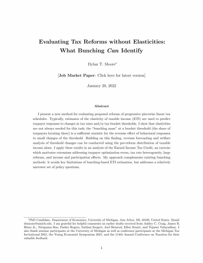
panel of the figure 1 depicts the budget set induced by this type of tax schedule. I will often refer

to z? as the “kink point” because, as the figure shows, this budget set features a convex kink at z?.

Taxpayer Choices Under Linear Tax Schedules

To characterize the choices that taxpayers make when facing tax schedule (2), we must first consider

the counterfactual choices they would make when facing the linear tax schedules T0 (z) and T1 (z).

These two tax schedules differ in both their marginal tax rates (t0 vs. t1) and their associated

virtual income (G vs. (t1 − t0) z? + G). Let z (t, V ; θ) be the choice of taxable income a type θ

taxpayer would make under a linear tax schedule with marginal tax rate t < 1 and virtual income

V ∈ R, and let H (z; t, V ) be the cumulative distribution function (CDF) of taxable income induced

11Assumption 1 implies that each taxpayer’s taxable income choices will satisfy the strong axiom of revealedpreference (SARP) because taxpayer preferences are rational and their choice of taxable income is always unique.This property allows for the simple characterization of taxpayer behavior presented later in equation (1).

7

by this linear tax schedule.12 For simplicity of exposition, I require that this CDF is continuously

differentiable in z.13

Assumption 2 (Regularity Condition). For any linear tax schedule with marginal tax rate t < 1

and virtual income V , the cumulative distribution function of taxable income induced by this schedule

(H (z; t, V )) is continuously differentiable for all z, with a corresponding density function h (z; t, V ).

In this section I will further assume that differences in the virtual income amount do not affect

taxpayer decisions: that is, there are no income effects. Later, I discuss the implications of income

effects for my results.

Assumption 3 (No Income Effects on Taxable Income Choices). Any pair of linear tax schedules

with the same marginal tax rate t induce the same distribution of taxable income, irrespective of

differences in demogrant amounts. That is, for any t < 1 and V, V ′ ∈ R,

H (z; t, V ) = H(z; t, V ′

)for all z.

Under this assumption, we can simplify notation somewhat, writing a type θ taxpayer’s choice under

a linear tax schedule with marginal rate t as z (t; θ), the corresponding CDF of taxable income as

H (z; t), and the corresponding density function as h (z; t). Importantly, note that the distribution

H (z; t1) is invariant to changes in the parameter z? that affect the virtual income associated with

T1, and that both H (z; t1) and H (z; t0) are invariant to changes in the demogrant amount G.

To further simplify notation, let zk (θ) ≡ z (θ, tk), Hk (z) ≡ H (z; tk), and hk (z) ≡ h (z; tk) for

k ∈ {1, 2}.12Formally, H (z; t, V ) ≡

∫1 {z (t, V ; θ) ≤ z} dF (θ).

13This assumption could be weakened somewhat. Obtaining my key results requires that the CDF of taxable incomeunder a linear tax schedule is continuously differentiable at a tax bracket threshold. However, these results are robustto the possibility that the CDF of taxable income under a linear tax features discontinuities or non-differentiability atincome levels away from the bracket threshold. Thus, the result is robust to the possibility that, for example, sometaxpayers have reference-dependent preferences that induce bunching at a reference point, as long as this referencepoint is not located at the tax bracket threshold and is unaffected by changes to the threshold.

8

Taxpayer Choices under a Two-Bracket Tax Schedule

When facing the two-bracket tax schedule (2), the choice of taxable income for any taxpayer type θ

can be written as:14

z (θ) =

z0 (θ) if z0 (θ) < z?

z1 (θ) if z1 (θ) > z?

z? if z1 (θ) ≤ z? ≤ z0 (θ)

. (5)

The lower panel of figure 1 illustrates this visually, showing how taxpayers make decisions when

facing the two-bracket tax schedule (2). All taxpayers will choose to earn income up to the point

where the marginal cost of earning exceeds the marginal benefit. For some, this means locating in

the interior of the lower bracket and choosing to earn the same amount of income they earn would

under T0. For others, this means locating in the interior of the upper bracket and earning the same

amount they would under T1.

However, not all taxpayers’ choices can be characterized this way. The kink in the tax schedule

induces a discontinuous drop in the marginal benefit of income at z?. Consequently, some taxpayers’

marginal cost curves pass through the discontinuity, never intersecting the marginal benefit. For

such taxpayers, the marginal benefit of earning each dollar of income below z? exceeds their marginal

cost but for each dollar beyond z? the opposite is true.15 Thus, they will locate at exactly z?. These

taxpayers are bunchers.

Figure 2 shows how the choices of a population of different types of taxpayers facing the tax schedule

(2) generate a distribution of taxable income which features “bunching” at the kink point. As in

figure 1, the upper panel of figure 2 depicts how taxpayers make choices by plotting the marginal

benefit of income against the marginal cost curves of different types of taxpayers. The lower panel

of the figure shows the CDF of taxable income H that is induced type distribution F and the

type-to-choice mapping z (·) (equation 5). Below the kink point, the observed CDF of taxable

income coincides with the CDF under the linear tax schedule T0 (H0), and above this point it

coincides with the CDF under the linear tax schedule T1 (H1):

H (z) =

H0 (z) if z < z?

H1 (z) if z ≥ z?(6)

Importantly, this CDF features a discontinuity in the CDF of taxable income at z? (as shown in

Figure 2). This is the bunching mass: the fraction of agents who would prefer to locate above the

14All taxpayers must satisfy one, and only one, of the three conditions in equation (5). The alternative possibility(z (t0; θ) < z? < z (t1; θ)) would violate SARP, as z (t0; θ) would be affordable under T1 and z (t1; θ) would be affordableunder T0. As Assumption 1 implies that SARP must be satisfied, this is not possible.

15Put another way, if such taxpayers faced the linear tax schedule T0 they would want to locate above the kink, butif they faced a linear tax schedule T1 they would want to locate below the kink.

9

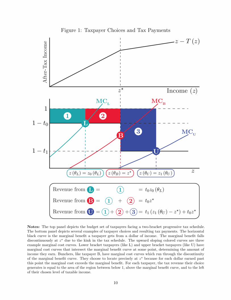
Figure 1: Taxpayer Choices and Tax Payments

U

B

L

Income (z)

Aft

er-T

ax I

ncom

e

MCL

z

z�

z (θB) = z�

z − T (z)

1 2

MCB

MCU31− t0

1− t1

1

z (θL) = z0 (θL) z (θU ) = z1 (θU )

t1 (z1 (θU )− z�) + t0z

�

Revenue from L = =

Revenue from L = + =

Revenue from L = 1 + + =

L 1

1B 2

1 2U 3

t0z0 (θL)

t0z�

Notes: The top panel depicts the budget set of taxpayers facing a two-bracket progressive tax schedule.The bottom panel depicts several examples of taxpayer choices and resulting tax payments. The horizontalblack curve is the marginal benefit a taxpayer gets from a dollar of income. The marginal benefit fallsdiscontinuously at z? due to the kink in the tax schedule. The upward sloping colored curves are threeexample marginal cost curves. Lower bracket taxpayers (like L) and upper bracket taxpayers (like U) havemarginal cost curves that intersect the marginal benefit curve at some point, determining the amount ofincome they earn. Bunchers, like taxpayer B, have marginal cost curves which run through the discontinuityof the marginal benefit curve. They choose to locate precisely at z? because for each dollar earned pastthis point the marginal cost exceeds the marginal benefit. For each taxpayer, the tax revenue their choicegenerates is equal to the area of the region between below 1, above the marginal benefit curve, and to the leftof their chosen level of taxable income.

10

kink point under T0, but below the kink point under T1:16

Pr {z1 (θ) < z? < z0 (θ)} = H1 (z?)−H0 (z?) . (7)

Figure 2 provides some intuition for why bunching occurs, depicting a set of taxpayers who would

all make distinct choices under a linear tax schedule, but many of whom lump together at z? when

facing a kinked tax schedule.

Note that this presentation ignores important complications that arise in real-world bunching

applications due to frictions in taxpayer income choices. Taxable income data are not usually

consistent with so-called “sharp” bunching: a large group of taxpayers locating at precisely the kink

point. Rather, evidence of bunching usually comes in the form of a diffuse clustering of taxpayers

around a kink. Consistent with the existing literature on bunching methodology, I derive my main

results by abstracting from such concerns and revisit them in section 3.

1.2 The Bunching Mass as a Sufficient Statistic

Without loss of generality, suppose that G = 0. Under assumptions 1–3, tax revenue under the

kinked tax schedule (2) is simply:

R (z?) ≡ t0

∫ z?

0zh0 (z) dz︸ ︷︷ ︸

revenue below the kink

+ t0z? (H1 (z?)−H0 (z?))︸ ︷︷ ︸revenue from bunchers

+

∫ ∞z?

[t1 (z − z?) + t0z?]h1 (z) dz︸ ︷︷ ︸

revenue above the kink

. (8)

The lower panel of figure 2 depicts tax revenue graphically.

Theorem 1 presents the identification result that provides the foundation of this paper, which can

be derived immediately by differentiating the revenue function R (z?). However, this provides little

intuition for the result. Here, I present a graphical derivation to provide a deeper understanding of

this key finding. Appendix C.1 presents an alternative heuristic derivation.

Now, consider a tax reform displayed in figure 3, which lowers the bracket threshold from z? to z′.

This reform discretely increases the marginal tax rate in the interval (z′, z?] while simultaneously

reducing the demogrant (virtual income) associated with the second tax bracket. Figure 4 visually

depicts how such a reform would change taxpayer choices, and the resulting the revenue effects.

Taxpayers can be broken into five groups that differ in how they are affected by the reform. Persistent

lower bracket taxpayers are those with pre-reform income below the new kink point (z0 (θ) ≤ z?).Their choice remains optimal after the reform so they do not change their behavior in response to it.

Similarly, persistent upper bracket taxpayers—those with a pre-reform income (z1 (θ) > z′)—will

not respond to the reform if there are no income effects (assumption 3).

16The name of this parameter reflects the fact that in the density of taxable income, bunching behavior manifestsas a mass point at z?.

11

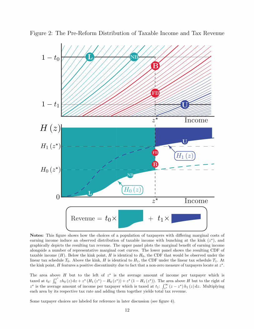
Figure 2: The Pre-Reform Distribution of Taxable Income and Tax Revenue

U

FB

BNBL1− t0

1− t1

z� Income

z� Income

H0 (z�)

H1 (z�)

0

H (z)

U

FB

B

L

NB

Revenue = +t0× t1×

Notes: This figure shows how the choices of a population of taxpayers with differing marginal costs ofearning income induce an observed distribution of taxable income with bunching at the kink (z?), andgraphically depicts the resulting tax revenue. The upper panel plots the marginal benefit of earning incomealongside a number of representative marginal cost curves. The lower panel shows the resulting CDF oftaxable income (H). Below the kink point, H is identical to H0, the CDF that would be observed under thelinear tax schedule T0. Above the kink, H is identical to H1, the CDF under the linear tax schedule T1. Atthe kink point, H features a positive discontinuity due to fact that a non-zero measure of taxpayers locate at z?.

The area above H but to the left of z? is the average amount of income per taxpayer which is

taxed at t0:∫ z?

0zh0 (z) dz + z? (H1 (z?)−H0 (z?)) + z? (1−H1 (z?)). The area above H but to the right of

z? is the average amount of income per taxpayer which is taxed at t1:∫∞z? (z − z?)h1 (z) dz. Multiplying

each area by its respective tax rate and adding them together yields total tax revenue.

Some taxpayer choices are labeled for reference in later discussion (see figure 4).

12

Figure 3: Lowering a Tax Bracket Threshold

Income (z)

Aft

er-T

ax I

ncom

e

z − T (z)

z�

z′

By contrast, taxpayers with pre-reform income in the interval (z′, z?] will respond to the reform.

Some are persistent bunchers: those who find it optimal to bunch both before and after the reform,

reducing their income from z? to z′ (z0 (θ) > z? and z1 (θ) < z′). However, not all pre-reform

bunchers will choose to continue to bunch. Any pre-reform bunchers with z1 (θ) ∈ (z′, z?) will find it

optimal to leave the bunching mass after the reform, choosing instead to reduce their taxable income

from z? to z1 (θ). I call this group the former bunchers. Finally, there is a group of taxpayers with

z0 (θ) ∈ (z′, z?), who initially have incomes between the new kink point and the old kink. They find

it optimal to locate at the new kink point post-reform, reducing their income from z0 (θ) to z′. I

call this group the new bunchers.

The mechanical effect of the reform is the additional tax revenue that results from taxing incomes

in the interval (z′, z?] at an increased marginal tax rate of t1 (relative to a pre-reform tax rate of

t0). As figure 4 shows, any taxpayers with post-reform incomes above z′ contribute to this effect;

this group includes both the persistent upper bracket taxpayers and former bunchers. Formally, the

mechanical effect can be written as

(t1 − t0)

[(z? − z′

)(1−H1 (z?)) +

∫ z?

z′

(z − z′

)h1 (z) dz

]︸ ︷︷ ︸

= area of blue region in figure 4

. (9)

The behavioral response effect of the reform is the loss of tax revenue caused by taxpayers reducing

their taxable income in response to the increase in the marginal tax rate in the interval (z′, z?].

As figure 4 shows, any taxpayers with pre-reform incomes in the interval (z′, z?] contribute to this

effect. This includes the persistent bunchers, former bunchers, and new bunchers. Formally, the

13

Figure 4: Revenue Effects of Decreasing a Kink Point

1− t0

1− t1

Income

z� Income

H0 (z�)

H1 (z�)

0

U

L

FB

B

NB

z′

NB

B

FB

H0 (z′)

H1 (z′)

z′

FB

B

NB

L

FB

NB

B

z�

(t1 − t0)× −t0×

Behavioral Response E�ectMechanical E�ect

U

H (z)

Notes: This figure visually depicts the effect of reducing the bracket threshold from z? to z′. In the toppanel, the five labeled taxpayer choices are each representative of a particular class of taxpayers. Theselabels are also in figure 2 for reference. Persistent lower bracket taxpayers (L) and persistent upper brackettaxpayers (U); their behavior is unaffected by the reform. However, some taxpayers do respond to thereform. Persistent bunchers (B) bunch both before and after the reform, responding by reducing theirincome from z? to z′. New bunchers (NB) previously had incomes in the interval (z′, z?) but reduce thisto z′, joining the new bunching mass. Former bunchers (FB) are induced to exit the bunching massas a result of the reform, reducing their income from the old kink point z? to some value in the interval (z′, z?).

The mechanical effect is the additional revenue that results from taxing income in the interval(z′, z?] at a higher rate. Taxpayers like U and FB contribute to this effect. The behavioral response effect isthe revenue that is lost because some taxpayers in the (z′, z?] reduce their taxable income. Taxpayers like B,NB, and FB all contribute to this effect.

14

behavioral response effect can be written as

− t0

[∫ z?

z′

(z − z′

)h0 (z) dz +

(z? − z′

) (H1

(z′)−H0 (z?)

)+

∫ z?

z′(z? − z)h1 (z) dz

]︸ ︷︷ ︸

= area of red region in figure 4

. (10)

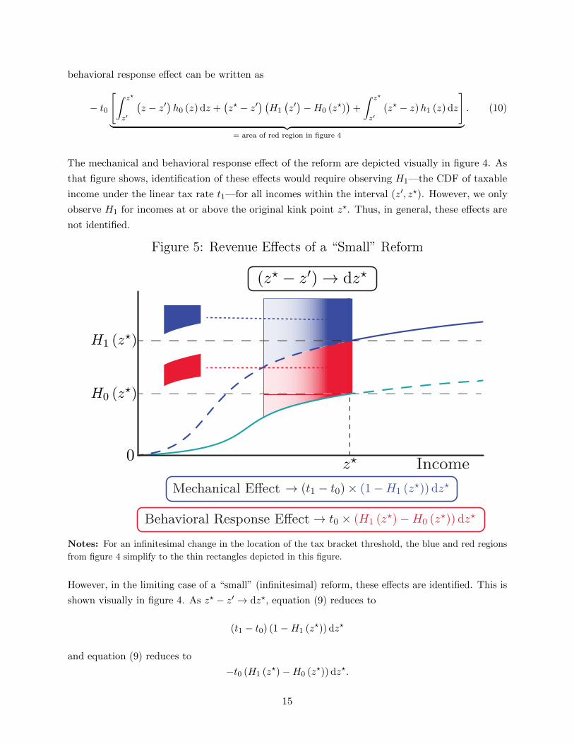
The mechanical and behavioral response effect of the reform are depicted visually in figure 4. As

that figure shows, identification of these effects would require observing H1—the CDF of taxable

income under the linear tax rate t1—for all incomes within the interval (z′, z?). However, we only

observe H1 for incomes at or above the original kink point z?. Thus, in general, these effects are

not identified.

Figure 5: Revenue Effects of a “Small” Reform

z� Income

H0 (z�)

H1 (z�)

0

Mechanical E�ect

(z�− z

′) → dz

�

Behavioral Response E�ect

Notes: For an infinitesimal change in the location of the tax bracket threshold, the blue and red regions

from figure 4 simplify to the thin rectangles depicted in this figure.

However, in the limiting case of a “small” (infinitesimal) reform, these effects are identified. This is

shown visually in figure 4. As z? − z′ → dz?, equation (9) reduces to

(t1 − t0) (1−H1 (z?)) dz?

and equation (9) reduces to

−t0 (H1 (z?)−H0 (z?)) dz?.

15

Notice that the fraction of taxpayers with incomes above the kink (1−H1 (z?)) and the discontinuity

of the CDF of taxable income at the kink (H1 (z?)−H0 (z?)) are features of the observed distribution

of taxable income. This leads to the key identification result of this paper.

Theorem 1 (Sufficiency of the Bunching Mass). Under assumptions 1, 2, and 3, if the tax schedule

is piecewise linear with two tax brackets (as defined in equation 2), then the first-order revenue effect

of decreasing the kink point z? is

−R′ (z?) = (t1 − t0) (1−H1 (z?))︸ ︷︷ ︸mechanical effect

−t0

bunching mass︷ ︸︸ ︷(H1 (z?)−H0 (z?))︸ ︷︷ ︸

behavioral response effect

. (11)

The bunching mass is a sufficient statistic for the revenue impact of the behavioral response to the

reform. The probability of locating above the kink is a sufficient statistic for the mechanical revenue

effects of the reform.

2 Evaluation without Elasticities

In this section, I build on Theorem 1 to demonstrate how bunching designs can be used to evaluate

proposed reforms to progressive piecewise linear tax schedules. I discuss how Theorem 1 can be used

to estimate the revenue impact of a prospective tax reform and compare this approach to existing

techniques for predicting the revenue effects of tax reforms, showing that these techniques do not

correctly account for the effect of changing tax brackets. Following this discussion, I consider the

application of Theorem 1 to welfare analysis. First, I present a novel test for the Pareto efficiency

of an observed tax schedule. This amounts to a test of whether a given tax schedule is locally on

the wrong side of the Laffer curve, so that a local tax increase (implemented by decreasing a tax

bracket threshold) would actually decrease revenue. Next, I characterize the welfare effects of this

reform according to standard welfarist objective functions.

2.1 Revenue Forecasting

Consider an economy facing the tax schedule from two-bracket tax schedule (2). Let (t0, t1, z?) be

the parameters of the current tax schedule and consider a reform which changes these parameters

to the new values (t0 + ∆t0, t1 + ∆t, z? −∆z?). Suppose—without loss of generality—that ∆z? > 0

so that this reform results in a lower bracket threshold. One way to estimate the revenue effect of

16

this reform is to use a first-order Taylor approximation. The approximation can then be written as

∆R ≈ (t1 − t0) (1−H1 (z?)) ∆z?︸ ︷︷ ︸mechanical effect of

threshold change

−t0 (H1 (z?)−H0 (z?)) ∆z?︸ ︷︷ ︸behavioral response effect

of threshold change

+∂R

∂t0∆t0 +

∂R

∂t1∆t1︸ ︷︷ ︸

rate change effects

(12)

Letting εc ≡ −1−tz

∂z∂(1−t) denote the elasticity of taxable income (ETI), the partial effect of changing

the lower bracket tax rate is

∂R

∂t0= E [z|z < z?]H0 (z?) + z? (1−H0 (z?))︸ ︷︷ ︸

mechanical effect

− t01− t0

E [zεc|z < z?]H0 (z?)︸ ︷︷ ︸behavioral response effect

, (13)

and the partial effect of changing the upper bracket tax rate is

∂R

∂t1= E [z − z?|z > z?] (1−H1 (z?))︸ ︷︷ ︸

mechanical effect

− t11− t1

E [zεc|z > z?] (1−H1 (z?))︸ ︷︷ ︸behavioral response effect

. (14)

Equation (12) makes clear that not every aspect of tax reform evaluation requires knowledge of

taxpayer elasticities. The part of the reform effect which is caused by tax bracket changes can be

estimated relying only on features of the pre-reform distribution of taxable income. On the other

hand, equation (12) also shows that predicting the revenue effect of changing rates within a bracket

does require having some knowledge of the taxpayer ETIs, as equations (13) and (14) contain terms

which depend on these elasticities.

To understand the value of this insight, it is helpful to compare equation (12) to current practices

for predicting the effect of tax policy reforms. Analysts in some government agencies and think

tanks have adopted the practice of estimating the behavioral response effect of any proposed tax

reform using an elasticity-based approach, as follows:17

behavioral response effect ≈ −∑i

∆EMTRi ·EMTRi

1− EMTRi· zi · εci

where EMTRi is the effective marginal tax rate of taxpayer i, ∆EMTRi is the change in their

effective marginal rate induced by the reform, zi is pre-reform taxable income, and εci is the assumed

ETI of taxpayer i. Applying this approach to approximate the revenue effect of a tax reform would

yield the following expression

17For example, the Government of Canada’s Parliamentary Budget Office appears to follow this practice whenestimating revenue effects of proposed tax reforms, including reforms that induce bracket changes (http://www.pbo-dpb.gc.ca/web/default/files/files/files/Fiscal Impact and Incidence EN.pdf). More generally, I have found thatorganizations that report the results of similar revenue forecasting exercises do not provide precise informationabout the methodological approach used, though many such reports provide vague descriptions of “elasticity-basedestimation”.

17

∆R ≈ ∂R

∂t0∆t0 +

∂R

∂t1∆t1︸ ︷︷ ︸

rate change effects

+ (t1 − t0) (1−H1 (z?)) ∆z?︸ ︷︷ ︸mechanical effect of threshold change

− t01− t0

(t1 − t0)E [zεc|z ∈ [z? −∆z?, z?]] (H1 (z?)−H0 (z? −∆z?))︸ ︷︷ ︸behavioral response effect of threshold change

(15)

The elasticity-based approach approximates the effect of rate changes the same way equation (12)

does, but differs markedly in how it accounts for the impact of bracket changes. The elasticity-based

approach treats bracket changes as simply another way of changing marginal tax rates over some

range of income, and attempts to use elasticities to approximate the behavioral response to these

rate changes.18

My results show that this reliance on elasticities is unnecessary. Given the internal and external

validity challenges associated with ETI estimates, this finding is potentially of considerable policy-

relevance. Moreover, the elasticity-based approximation of the behavioral response effect of a bracket

change is biased. Even if the correct elasticities were plugged into equation (15), the resulting

prediction of the behavioral response effect of the bracket change should not be expected to coincide

with a prediction based on equation (12).19

An important caveat to the application of equation (12) is that it is only a first-order approximation,

and so its predictions about the impact of discrete policy changes will have errors. Appendix

A discusses these errors in detail, as well as possible methods for improving on the first-order

approximation. For example, higher-order Taylor approximations of the revenue effects of moving a

bracket threshold are also identified by the observed distribution of taxable income.20 Appendix

A also discusses the possibility of a partial identification approach, suggesting one way to bound

discrete reform revenue effects. Finally, in the empirical application in section 3.3, I present estimated

18In particular, this approach estimates the behavioral responses of taxpayers by first calculating how the reformwill alter the marginal tax rates of taxpayers who fall between the old bracket threshold and the new threshold andthen multiplying this change by ∂z

∂t= − zεc

1−t0. These estimated responses are multiplied by the pre-reform marginal

tax rate t0 to obtain the estimated revenue effect.19To be more precise about the “bias” inherent in the elasticity-based approach of equation (15), note that a

valid first-order approximation to the effect of a reform should be exact in the limit of a small reform. This is truefor the approximation presented in equation (12) by construction. Consequently, we can assess the validity of theapproximation of equation (15) by checking to see whether it delivers the same predicted revenue effect in the limitingcase of a small bracket change. This would require that

lim∆z?→0

− t01−t0

(t1 − t0)E [zεc|z ∈ [z? −∆z?, z?]] (H1 (z?)−H0 (z? −∆z?))

∆z?= −t0 (H1 (z?)−H0 (z?))

However, for any t0 6= 0, the limit on the left-hand side of the equation above diverges to negative infinity, so thiscondition cannot hold. Thus, equation (15) is not a valid first-order approximation to the revenue effect of a taxreform that changes tax brackets.

20This result parallels some results from the literature on regression discontinuity designs (RDD). The usualparameter of interest in such designs is the average treatment effect at the cutoff (ATEC), which is well known to benonparametrically identified under standard conditions. Dong and Lewbel (2015) show that partial derivatives of theATEC with respect to the location of the treatment cutoff are also identified.

18

revenue effects of a discrete reform based on a simple polynomial extrapolation method.

2.2 Testing Pareto Efficiency

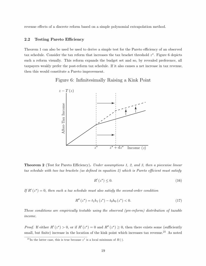
Theorem 1 can also be used be used to derive a simple test for the Pareto efficiency of an observed

tax schedule. Consider the tax reform that increases the tax bracket threshold z?. Figure 6 depicts

such a reform visually. This reform expands the budget set and so, by revealed preference, all

taxpayers weakly prefer the post-reform tax schedule. If it also causes a net increase in tax revenue,

then this would constitute a Pareto improvement.

Figure 6: Infinitesimally Raising a Kink Point

Income (z)

Aft

er-T

ax I

ncom

e

z − T (z)

z�

z� + dz

�

Theorem 2 (Test for Pareto Efficiency). Under assumptions 1, 2, and 3, then a piecewise linear

tax schedule with two tax brackets (as defined in equation 2) which is Pareto efficient must satisfy

R′ (z?) ≤ 0. (16)

If R′ (z?) = 0, then such a tax schedule must also satisfy the second-order condition

R′′ (z?) = t1h1 (z?)− t0h0 (z?) < 0. (17)

These conditions are empirically testable using the observed (pre-reform) distribution of taxable

income.

Proof. If either R′ (z?) > 0, or if R′ (z?) = 0 and R′′ (z?) ≥ 0, then there exists some (sufficiently

small, but finite) increase in the location of the kink point which increases tax revenue.21 As noted

21In the latter case, this is true because z? is a local minimum of R (·).

19

above, this would constitute a Pareto-improving reform. Theorem 1 shows that R′ (z?) can be

identified from the observed distribution of taxable income. It emerges that R′′ (z?) can also be

identified because the density terms that appear on the right-hand side of equation (17)—while not

directly observable—are limit points of the observed income density.22

Theorem 2’s test of Pareto efficiency is an analogue of the test for local Laffer effects initially

proposed by Werning (2007). However, no prior implementations of such tests can account for

the behavioral response to taxation without committing to a specific model of taxpayer behavior

and calibrating model parameters. By contrast, this test accounts for the behavioral response to

changing tax bracket thresholds without using any information beyond the observed distribution of

taxable income. The robustness of this test comes at the cost of the scope of inquiry, as the test is

uninformative about other tax reforms of interest.

In appendix B, I expand on the above Pareto efficiency test, constructing additional testable

conditions for efficiency using an analogue of the two-bracket reforms discussed by Bierbrauer, Boyer,

and Hansen (2020).

2.3 Welfare Effects of Moving Kinks

The efficiency results above demonstrate that bunching can be used to provide a nonparametric test

of the Pareto principle, but efficiency is a very weak normative criterion. It is also of interest to

consider welfare effects under a stronger definition of welfare.

The sharpest welfare effect results are obtained by assuming a Rawlsian (revenue-maximizing)

objective. A Rawlsian planner has no reason to forgo any revenue gains, irrespective of whether

these come at the cost of some agents’ private welfare.23

22Specifically, h0 (z?) can be identified as a limit point of the observed density from below the kink

limz→z?−

h (z) = limz→z?

h0 (z) = h0 (z?)

and h1 (z?) as a limit point of the observed density from above the kink

limz→z?+

h (z) = limz→z?

h1 (z) = h1 (z?) .

23Here, I am adopting the standard optimal tax theory convention of labeling the maximin objective

max

{minθ∈Θ

u (c (θ) , z (θ) ; θ)

}as a “Rawlsian” welfare maximization problem. I also adopt the standard assumption that this maximization problemis equivalent to

max

{minθ∈Θ

c (θ)

},

so that the agent with the lowest level of utility is the agent with the lowest level of consumption. Further assumingthat the marginal dollar of tax revenue finances increases in the demogrant G, the social planner’s problem reduces toone of revenue maximization.

20

Theorem 3 (Test for Rawlsian Optimality). Under assumptions 1, 2, and 3, a piecewise linear

tax schedule with two tax brackets (as defined in equation 2) which is Rawlsian-optimal (revenue-

maximizing) must satisfy

R′ (z?) = 0, (18)

and

R′′ (z?) = t1h1 (z?)− t0h0 (z?) < 0. (19)

This theorem simply states that the location of a kink point in a revenue-maximizing tax schedule

must satisfy standard necessary and sufficient conditions for a local maximum.24 As in theorem 2,

the second-order condition (19) ensures that the kink is not located at a local minimum.

2.3.1 Bergsonian Welfare Functions

Next, consider the case where the planner may have some reason to forgo revenue-increasing tax

reforms. For this discussion, it will be helpful to first reframe the finding presented in Theorem 1 in

the language of fiscal externalities. The fiscal externality of a given tax reform is the ratio of the

behavior response effect to the mechanical effect of the reform. This metric provides an intuitive

summary of the efficiency costs of a reform, reflecting the revenue loss due to the behavioral response

per dollar raised through the mechanical effect of the reform.

Corollary 1 (Fiscal Externality is Identified). Under assumptions 1, 2, and 3, if the tax schedule

is piecewise linear with two tax brackets (as defined in equation 2), then the fiscal externality (FE)

of marginally decreasing the kink point z? is

FE (z?) ≡ − t0 (H1 (z?)−H0 (z?))

(t1 − t0) (1−H1 (z?)), (20)

and is identified by the observed (pre-reform) distribution of taxable income.

Suppose we adopt a standard, additively separable Bergsonian welfare function as our measure of

social welfare in a society with a two bracket tax schedule like that defined in equation (2). That is,

suppose that social welfare when the kink point is located at z? is

W (z?) ≡∫ω (v (θ; z?)) dF (θ)

λ+R (z?) , (21)

where v (θ; z?) is the indirect utility function of a type θ agent, λ is the marginal social value of

government revenue, and ω (·) is some weakly increasing, weakly convex function of utility.

24Note, theorem 3 does not provide a test for whether the kink point is at a globally revenue-maximizing location,as R (z?) need not be a strictly concave function in general.

21

I define the marginal rate of substitution for a type θ agent earning income z as

MRS (z, θ) ≡ −∂u(c,z;θ)/∂z∂u(c,z;θ)/∂c

,

where consumption c ≡ z − T (z). Further, I shall denote the marginal social welfare weight of a

type θ agent as

g (θ) ≡ ω′ (v (θ; z?))

λ

∂u (c, z; θ)

∂c.

The welfare weight reflects the marginal social value of a dollar of private consumption for a type θ

agent.

I assume that the marginal dollar of government revenue is used to finance increases in the demogrant

(or something with equivalent marginal social value). Thus, given the above definition, the average

marginal social welfare weight is ∫g (θ) dF (θ) = 1.

That is to say the marginal social value of a dollar of government revenue is one.25

The first-order welfare effect of decreasing the location of the kink point can then be written as

−W ′ (z?) = (t1 − t0)

∫ ∞z?

(1− g (z))h1 (z) dz︸ ︷︷ ︸mechanical effect

−t0 (H1 (z?)−H0 (z?))︸ ︷︷ ︸revenue effect of behavioral response

−∫{θ:z1(θ)<z?<z0(θ)}

g (θ) (1− t0 −MRS (z?, θ)) dF (θ)︸ ︷︷ ︸utility effect of behavioral response

(22)

where g (z) ≡ E [g (θ) |z (θ) = z] is the average marginal social welfare weight of agents with an

income of z under the current tax schedule.

Notice that the first-order welfare effect of decreasing the location of a kink point differs from most

similar expressions found in the optimal tax literature, because the behavioral response to this

reform has a first-order effect on welfare for individuals in the bunching mass. To understand why,

recall that the absence of such first-order welfare effects depends critically on the envelope theorem.

But for bunchers, the envelope condition need not be satisfied.26 In particular, for at least some

types of agents who choose to bunch, we have

1− t0 −MRS (z?, θ) > 0. (23)

Thus, reducing the location of the kink point has a first-order welfare effect because it has a

25The marginal cost of increasing the demogrant is 1 and the marginal social benefit is∫g (θ) dF (θ). They must be

equalized in the optimal tax system.26Figure 1 shows this visually. The marginal cost curve of a typical buncher does not intersect the marginal benefit

function; rather, it runs through the discontinuity in this function at z?. Thus, their marginal benefit of earningexceeds their marginal cost at z?: the envelope condition fails.

22

first-order effect on the private welfare of bunchers, decreasing utility by

(1− t0 −MRS (z?, θ))∂u

∂c

for any type θ who is currently bunching and continues to bunch following the reform. The third

term of equation (22) multiplies this utility effect by G′ (V (θ; z?)) and integrates over all agents

who are bunching to obtain the total first-order welfare effect.27

The exception to the general failure of the envelope theorem are the so-called marginal bunchers

that Saez (2010) used to motivate his original bunching method. These are taxpayers who choose

to locate at z? under both the observed tax schedule (z (θ) = z?) and the counterfactual linear tax

schedule with tax rate t0 (z0 (θ) = z?). For such individuals, the envelope condition holds

1− t0 −MRS (z?, θ) = 0.

Notice that these marginal bunchers can also be thought of as representing the new bunchers who

will enter the bunching mass following an infinitesimal decrease in the location of the kink point.

This explains why equation (22) does not include any terms accounting for the welfare implications

of the new buncher effect : for an infinitesimal change, there are no such effects to account for.

By contrast, the former buncher effect does have welfare implications, and these are accounted for

in equation (22). Former bunchers represent a second type of marginal buncher. For an infinitesimal

reform, the former bunchers are taxpayers who choose to locate at z? under both the observed tax

schedule (z (θ) = z?) and the counterfactual linear tax schedule with tax rate t1 (z1 (θ) = z?). This

implies that the indifference curves of the former bunchers are tangent to the slope of the higher

tax bracket before the reform,

1− t1 −MRS (z?, θ) = 0.

Thus, the first-order effect of the reform on their utility is the same as for taxpayers located above

z?:

(1− t0 −MRS (z?, θ))∂u

∂c= (t1 − t0)

∂u

∂c.

Building on these results, below I present an empirical test of welfarist optimality of the observed

tax schedule given a known function describing the average marginal social welfare weight at each

income level g (·). Before doing so, I will introduce one additional piece of helpful notation. Let

g+ (z) ≡ E [g (θ) |z (θ) > z]

=

∫ ∞z

g (z)h (z) dz

be the average marginal social welfare weight of taxpayers with income above the kink point.

27In the optimal tax theory literature, this type of first-order welfare effect usually only appears in the presenceof some kind of market failure. For example, externalities, labor market frictions, and behavioral biases can inducefirst-order welfare effects to behavioral responses to tax reforms.

23

Theorem 4 (Conditions for Welfarist-Optimality). Under assumptions 1, 2, and 3, a piecewise

linear tax schedule with two tax brackets (as defined in equation 2) which is welfare-maximizing

according to (21) must satisfy

1− g+ (z?)︸ ︷︷ ︸mechanical welfare effect

+

(1 +

t1 − t0t0

kg (z?)

)FE (z?)︸ ︷︷ ︸

behavioral response welfare effect

= 0 (24)

where

k ≡ E [g (θ) (1− t0 −MRS (z?, θ)) |z (θ) = z?]

g (z?) (t1 − t0)(25)

is the ratio of the true first-order welfare effect of the reform caused by the behavioral response of

bunchers relative to the upper bound of this effect: g (z?) (t1 − t0).

If the left-hand side of equation (4) is positive (negative), then there exists a welfare-improving

decrease (increase) of the kink point.

To gain some intuition about Theorem 4, consider what equation (24) would look like if the welfare

of the bunchers was irrelevant: g (z?) = 0. In this case, the condition simply states that at the

optimum the fiscal externality of the reform must be equal to the average gain in social welfare

caused by the mechanical effect of the reform. This average gain is the difference between the

marginal social value of a dollar of government revenue28 and the average marginal social value of a

dollar of private consumption for the agents who are impacted by the mechanical effects (which

is g+ (z?)). Thus, unlike in the Rawlsian case, at the optimum the social planner will sometimes

choose to forgo feasible revenue-increasing tax reforms because the redistributive benefits of the

reform may be insufficient to justify the welfare loss causes by the behavioral response to the reform

(as measured by the fiscal externality).

Returning to the general case, where g (z?) 6= 0, the fact that moving a kink point causes behavioral

responses which have a first-order welfare effect simply inflates the welfare implications of the fiscal

externality. This reflects the fact that the welfare loss caused by the behavioral response includes

both lost revenue and these first-order welfare impacts.

In general, the value of k is unidentified, so theorem 4 cannot be used as the basis for an empirical

test of the optimality of a tax schedule. However, given known values for the average welfare weight

parameters g+ (z?) and g (z?), we can obtain an empirical test motivated by a partial identification

approach to the problem.

28Recall that this is equal to one at the optimum.

24

Corollary 2 (Test for Welfarist-Optimality). Under assumptions 1, 2, and 3, a piecewise linear tax

schedule with two tax brackets (as defined in equation 2) which is welfare-maximizing according to

(21) must satisfy

1 +

(1 +

(t1 − t0t0

)g (z?)

)FE (z?) < g+ (z?) < 1 + FE (z?) . (26)

On the other hand, if

1 +

(1 +

(t1 − t0t0

)g (z?)

)FE (z?) ≥ g+ (z?)

then there exists a welfare-improving decrease of the kink point. If

1 + FE (z?) ≤ g+ (z?)

then there exists a welfare-improving increase of the kink point.

This test simply checks to make sure that condition (24) from theorem 4 is satisfied for at least one

k ∈ (0, 1). If there is no such value of k, then we can conclude that a welfare-improving movement

of the kink point exists. Importantly, a condition (24) is a necessary but insufficient condition for

welfare maximization.

3 Empirical Application

This section applies the ideas discussed above to revisit an empirical application from Saez (2010).

Saez applies his bunching methodology to estimate the ETI using a sample of US personal income tax

returns: the IRS Individual Public Use Tax Files. I use this same sample to revisit his investigation

of bunching at the first kink point of the Earned Income Tax Credit (EITC) schedule between 1995

and 2004.

During this period, the EITC provided a 34% subsidy on the marginal dollar of family earnings

in a single child household below $8580 (in 2008 $). The marginal subsidy for such a household

fell to zero at levels of earnings above these thresholds, introducing a convex kink in their budget

constraint. These households also faced a second convex kink point at earnings of $15740 (in 2008

$), above which the marginal subsidy became a marginal tax of 16%.

3.1 Filtering the Taxable Income Data

Before we can proceed with applying the results of section 2 to this dataset, we need to address the

matter of frictions in taxpayer choices. Recall that the results presented in the preceding sections

25

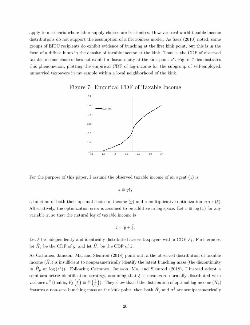
apply to a scenario where labor supply choices are frictionless. However, real-world taxable income

distributions do not support the assumption of a frictionless model. As Saez (2010) noted, some

groups of EITC recipients do exhibit evidence of bunching at the first kink point, but this is in the

form of a diffuse lump in the density of taxable income at the kink. That is, the CDF of observed

taxable income choices does not exhibit a discontinuity at the kink point z?. Figure 7 demonstrates

this phenomenon, plotting the empirical CDF of log-income for the subgroup of self-employed,

unmarried taxpayers in my sample within a local neighborhood of the kink.

Figure 7: Empirical CDF of Taxable Income

1.8 1.9 2 2.1 2.2 2.3 2.40.1

0.15

0.2

0.25

0.3

0.35

0.4

ECDF of z

For the purpose of this paper, I assume the observed taxable income of an agent (z) is

z ≡ yξ,

a function of both their optimal choice of income (y) and a multiplicative optimization error (ξ).

Alternatively, the optimization error is assumed to be additive in log-space. Let x ≡ log (x) for any

variable x, so that the natural log of taxable income is

z = y + ξ.

Let ξ be independently and identically distributed across taxpayers with a CDF Fξ. Furthermore,

let Hy be the CDF of y, and let Hz be the CDF of z.

As Cattaneo, Jansson, Ma, and Slemrod (2018) point out, a the observed distribution of taxable

income (Hz) is insufficient to nonparametrically identify the latent bunching mass (the discontinuity

in Hy at log (z?)). Following Cattaneo, Jansson, Ma, and Slemrod (2018), I instead adopt a

semiparametric identification strategy, assuming that ξ is mean-zero normally distributed with

variance σ2 (that is, Fξ

(ξ)≡ Φ

(ξσ

)). They show that if the distribution of optimal log-income (Hy)

features a non-zero bunching mass at the kink point, then both Hy and σ2 are semiparametrically

26

identified by Hz.29 For reference, appendix D.1 replicates their proof of this result.

Building on this identification strategy, Cattaneo, Jansson, Ma, and Slemrod (2018) propose a

method for estimating Hy and σ2 based on approximating the latent optimal income density function

hy using histograms. I propose an alternative method of estimation based approximating the latent

optimal income CDF (Hy) using two flexible polynomial functions. This method is briefly outlined

below. For a full description, see appendix D.2.

Let H0y be the distribution of log (y) under a linear tax schedule with tax rate t0 and let H1

y be the

distribution of log (y) under a linear tax schedule with tax rate t1. As shown in section 1.1, under

assumption 1 the distribution of log (y) under the two-bracket tax schedule is

Hy (y) ≡

H0y (y) if y ≤ log (z?)

H1y (y) if y > log (z?)

. (27)

The observed distribution of log-income is then given by

Hz (z) ≡∫ ∞z−log(z?)

H0y

(z − ξ

)dΦ

(ξ

σ

)+

∫ z−log(z?)

−∞H1y

(z − ξ

)dΦ

(ξ

σ

).

My estimation method approximates H0y (y) and H1

y (y) in the expression above using 8th-order

polynomial functions. Using a sample of taxpayers in a neighborhood of the kink point, I estimate

the coefficients of these polynomials via constrained minimization of simulated least squares. See

appendix D.2 for complete details.

I apply this filtering method independently for each of four subgroups of EITC eligible taxpayers:

unmarried employees, married employees, unmarried self-employed people, and married self-employed

people. Figure 8 shows the resulting estimate of the CDF Hy (y) for the subgroup of unmarried

self-employed taxpayers in my sample. This function is presented alongside the empirical CDF of

log-income (Hz (z)) and a simulated CDF of log-income based on the estimate function Hy (y) and

the estimated variance of errors σ2. In this case, the estimated model provides a good fit for the

data, with the simulated CDF closely tracking the empirical CDF.

Table 1: Estimated Bunching Mass & Share Above Kink by Subgroup

UnmarriedEmployees

Unmarried &Self-Employed

MarriedEmployees

Married &Self-Employed

H1 (z?)−H0 (z?) 0.004 0.079 0.002 0.0031−H1 (z?) 0.8543 0.7476 0.9732 0.9513

29In fact, Cattaneo, Jansson, Ma, and Slemrod (2018) present this finding under the assumption of normallydistributed optimization error that is additive in levels rather than in logs, but their identification result holds ineither case.

27

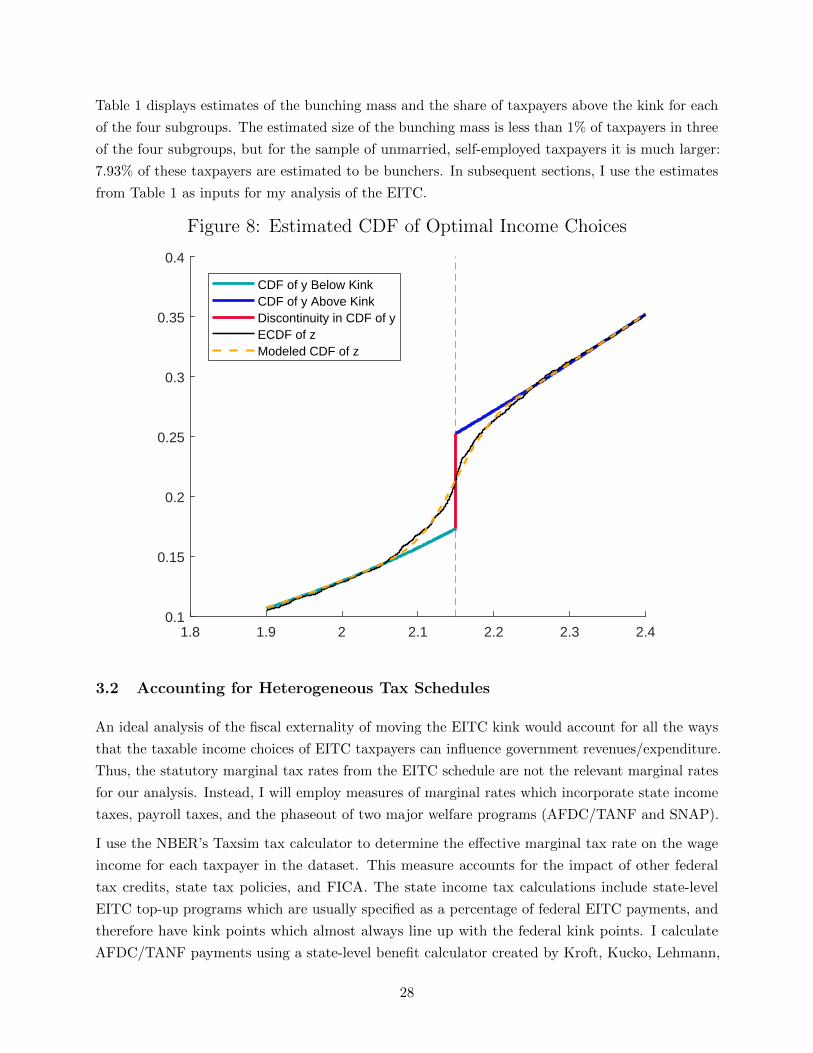
Table 1 displays estimates of the bunching mass and the share of taxpayers above the kink for each

of the four subgroups. The estimated size of the bunching mass is less than 1% of taxpayers in three

of the four subgroups, but for the sample of unmarried, self-employed taxpayers it is much larger:

7.93% of these taxpayers are estimated to be bunchers. In subsequent sections, I use the estimates

from Table 1 as inputs for my analysis of the EITC.

Figure 8: Estimated CDF of Optimal Income Choices

1.8 1.9 2 2.1 2.2 2.3 2.40.1

0.15

0.2

0.25

0.3

0.35

0.4

CDF of y Below KinkCDF of y Above KinkDiscontinuity in CDF of yECDF of zModeled CDF of z

3.2 Accounting for Heterogeneous Tax Schedules

An ideal analysis of the fiscal externality of moving the EITC kink would account for all the ways

that the taxable income choices of EITC taxpayers can influence government revenues/expenditure.

Thus, the statutory marginal tax rates from the EITC schedule are not the relevant marginal rates

for our analysis. Instead, I will employ measures of marginal rates which incorporate state income

taxes, payroll taxes, and the phaseout of two major welfare programs (AFDC/TANF and SNAP).

I use the NBER’s Taxsim tax calculator to determine the effective marginal tax rate on the wage

income for each taxpayer in the dataset. This measure accounts for the impact of other federal

tax credits, state tax policies, and FICA. The state income tax calculations include state-level

EITC top-up programs which are usually specified as a percentage of federal EITC payments, and

therefore have kink points which almost always line up with the federal kink points. I calculate

AFDC/TANF payments using a state-level benefit calculator created by Kroft, Kucko, Lehmann,

28

and Schmieder (2020). I use a crude approximation to the impact of SNAP (food stamps) which

assumes that a constant phase out rate of 20% applies throughout the relevant range of income,

following Kleven (2021).30

Importantly, effective marginal tax rates on either side of the first EITC kink may differ substantially

across the taxpayers in my analysis, as tax/benefit policy is not constant across states nor within

states across years. A valid empirical analysis therefore requires extending the baseline results

presented in sections 1 and 2. For simplicity, I will present a two bracket extension, though this can

be easily generalized to the multibracket case.

Suppose that type θ agents face the following two bracket tax schedule

T (z, z?; θ) ≡

t0 (θ) z if z ≤ z?

t1 (θ) z + [t0 (θ)− t1 (θ)] z? if z > z?,

where t0 (θ), and t1 (θ) are type-θ-specific tax schedule parameters.31 The first-order revenue effect

a tax reform which infinitesimally reduces z? is32

−R′ (z?) = E [t1 (θ)− t0 (θ) |z (θ) > z?] (1−H1 (z?))︸ ︷︷ ︸mechanical effect

−E [t0 (θ) |z1 (θ) < z? < z0 (θ)] (H1 (z?)−H0 (z?))︸ ︷︷ ︸behavioral response effect

. (29)

Results

The filtering method discussed in the previous section provides estimates of 1−H1 (z?) and H1 (z?)−H0 (z?). I estimate the expected tax rates on either side of the kink point—E [t0 (θ) |z0 (θ) = z?]

and E [t1 (θ) |z1 (θ) = z?]—via local linear regression. These estimates are presented in Table 2 for

each of the four subgroups discussed in 3.1. Contrary to what statutory federal income tax rates

would imply, effective marginal rates on either side of the EITC kink are positive for the average

taxpayer in my sample. This is consistent with the observation made by Bierbrauer, Boyer, and

Hansen (2020), who note that the negative marginal rates of the EITC are offset by the large

positive marginal rates induced by the phaseout of welfare benefits throughout most the relevant

range of income. Only in the case of unmarried, self-employed taxpayers is the marginal tax rate

30As in Kleven (2021) I assume a 54% take-up rate for both AFDC/TANF and SNAP.31This result can also be extended to cases where the kink point is a type-specific parameter.32The fiscal externality of this reform can be written as

FE ≡ −E [t0 (θ) |z1 (θ) < z? < z0 (θ)]

E [t1 (θ)− t0 (θ) |z (θ) > z?]

H1 (z?)−H0 (z?)

1−H1 (z?). (28)

29

just below the kink negative. The estimated size of the kink is also smaller than what statutory

EITC rates would imply for all subgroups.

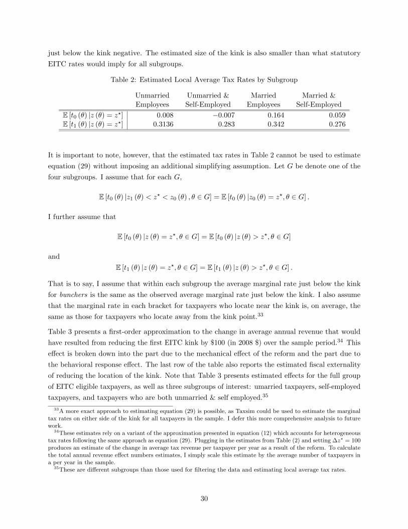
Table 2: Estimated Local Average Tax Rates by Subgroup

UnmarriedEmployees

Unmarried &Self-Employed

MarriedEmployees

Married &Self-Employed

E [t0 (θ) |z (θ) = z?] 0.008 −0.007 0.164 0.059E [t1 (θ) |z (θ) = z?] 0.3136 0.283 0.342 0.276

It is important to note, however, that the estimated tax rates in Table 2 cannot be used to estimate

equation (29) without imposing an additional simplifying assumption. Let G be denote one of the

four subgroups. I assume that for each G,

E [t0 (θ) |z1 (θ) < z? < z0 (θ) , θ ∈ G] = E [t0 (θ) |z0 (θ) = z?, θ ∈ G] .

I further assume that

E [t0 (θ) |z (θ) = z?, θ ∈ G] = E [t0 (θ) |z (θ) > z?, θ ∈ G]

and

E [t1 (θ) |z (θ) = z?, θ ∈ G] = E [t1 (θ) |z (θ) > z?, θ ∈ G] .

That is to say, I assume that within each subgroup the average marginal rate just below the kink

for bunchers is the same as the observed average marginal rate just below the kink. I also assume

that the marginal rate in each bracket for taxpayers who locate near the kink is, on average, the

same as those for taxpayers who locate away from the kink point.33

Table 3 presents a first-order approximation to the change in average annual revenue that would

have resulted from reducing the first EITC kink by $100 (in 2008 $) over the sample period.34 This

effect is broken down into the part due to the mechanical effect of the reform and the part due to

the behavioral response effect. The last row of the table also reports the estimated fiscal externality

of reducing the location of the kink. Note that Table 3 presents estimated effects for the full group

of EITC eligible taxpayers, as well as three subgroups of interest: umarried taxpayers, self-employed

taxpayers, and taxpayers who are both unmarried & self employed.35

33A more exact approach to estimating equation (29) is possible, as Taxsim could be used to estimate the marginaltax rates on either side of the kink for all taxpayers in the sample. I defer this more comprehensive analysis to futurework.

34These estimates rely on a variant of the approximation presented in equation (12) which accounts for heterogeneoustax rates following the same approach as equation (29). Plugging in the estimates from Table (2) and setting ∆z? = 100produces an estimate of the change in average tax revenue per taxpayer per year as a result of the reform. To calculatethe total annual revenue effect numbers estimates, I simply scale this estimate by the average number of taxpayers ina per year in the sample.

35These are different subgroups than those used for filtering the data and estimating local average tax rates.

30

Table 3: Revenue Effects of Reducing the First EITC Kink (Single Child Households, 1995-2004)

AllTaxpayers

Unmarried Self-EmployedUnmarried &Self-Employed

Mechanical Effect (2008 $) 38, 389, 708 12, 305, 422 13, 497, 845 2, 228, 590Behav. Response Effect (2008 $) −33, 569 4, 409 −3, 753 5, 614

Total Revenue Effect (2008 $) 38, 356, 139 12, 309, 832 13, 494, 092 2, 234, 204

Fiscal Externality −0.0009 0.0004 −0.0003 0.0025

Notes: The revenue effects reported in the first three rows of this table are first-order approxi-mations to the average additional revenue per year that would result from reducing the firstEITC kink by $100 (2008 $) based on equation (8).

The behavioral response effect is quite small relative to the mechanical effect in every case. This

can be seen most clearly in the small fiscal externality estimates, which suggest that for each dollar

raised through the mechanical effect of reducing the first EITC kink, about a tenth of a cent would

be lost to this behavioral response. Note as well that the behavioral response effect is actually

positive for unmarried taxpayers. and those taxpayers who are both unmarried and self-employed.

This happens because within these subgroups the average marginal tax rate just below the kink

is negative. Consequently, reducing the location of the first EITC kink causes both a mechanical

increase in revenue from all taxpayers above the kink who now receive a lower total subsidy amount

and an increase in revenue due to the behavioral response effect because moving the bunching

taxpayers to a lower taxable income reduces the subsidy they receive.

Theorem 2 provided conditions which must be satisfied in order for the observed tax schedule to be

plausibly welfare-optimal (ignoring income effects and extensive margin responses). One of these

conditions states that 1 + FE (z?) provides an upper bound on the average welfare weight above

the kink point (g+ (z?)). Thus, these results imply that we must have g+ (z?) < 1 to rationalize

observed tax policy as welfare-maximizing for the full group of EITC eligible taxpayers.

3.3 Discrete Reforms

One possible issue with the results presented in table 3 is that they are based on a first-order

approximation to the effect of a discrete reform that reduces the kink point by $100 (2008 $). As

noted in section 1.2, identification of discrete revenue effects of lowering a kink requires knowledge

of the unobserved values of H1 (z) between the old and new kink points. Appendix A discusses this

issue at length, as well as the similar issues that arise for a discrete reform which increases the kink

point.

One way to more precisely estimate of revenue effects is to estimate the unobserved values of H1 (z)

using the polynomial approximation obtained via the filtering procedure discussed in section 3.1.

Table 4 presents estimates based on this extrapolation method. The estimated revenue effects are

quite close to those presented in table 3. However, is important to note that while the filtering

31

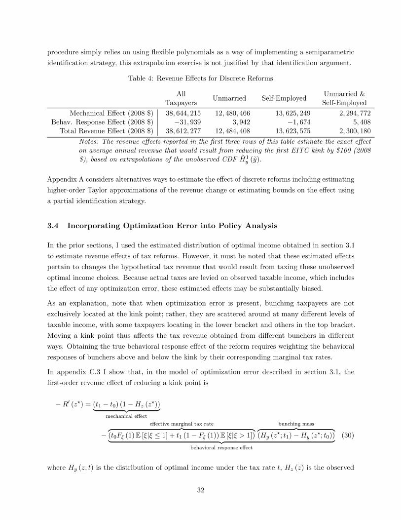
procedure simply relies on using flexible polynomials as a way of implementing a semiparametric

identification strategy, this extrapolation exercise is not justified by that identification argument.

Table 4: Revenue Effects for Discrete Reforms

AllTaxpayers

Unmarried Self-EmployedUnmarried &Self-Employed

Mechanical Effect (2008 $) 38, 644, 215 12, 480, 466 13, 625, 249 2, 294, 772Behav. Response Effect (2008 $) −31, 939 3, 942 −1, 674 5, 408

Total Revenue Effect (2008 $) 38, 612, 277 12, 484, 408 13, 623, 575 2, 300, 180

Notes: The revenue effects reported in the first three rows of this table estimate the exact effecton average annual revenue that would result from reducing the first EITC kink by $100 (2008$), based on extrapolations of the unobserved CDF H1

y (y).

Appendix A considers alternatives ways to estimate the effect of discrete reforms including estimating

higher-order Taylor approximations of the revenue change or estimating bounds on the effect using

a partial identification strategy.

3.4 Incorporating Optimization Error into Policy Analysis

In the prior sections, I used the estimated distribution of optimal income obtained in section 3.1

to estimate revenue effects of tax reforms. However, it must be noted that these estimated effects

pertain to changes the hypothetical tax revenue that would result from taxing these unobserved

optimal income choices. Because actual taxes are levied on observed taxable income, which includes

the effect of any optimization error, these estimated effects may be substantially biased.

As an explanation, note that when optimization error is present, bunching taxpayers are not

exclusively located at the kink point; rather, they are scattered around at many different levels of

taxable income, with some taxpayers locating in the lower bracket and others in the top bracket.

Moving a kink point thus affects the tax revenue obtained from different bunchers in different

ways. Obtaining the true behavioral response effect of the reform requires weighting the behavioral

responses of bunchers above and below the kink by their corresponding marginal tax rates.

In appendix C.3 I show that, in the model of optimization error described in section 3.1, the

first-order revenue effect of reducing a kink point is

−R′ (z?) = (t1 − t0) (1−Hz (z?))︸ ︷︷ ︸mechanical effect

−effective marginal tax rate︷ ︸︸ ︷

(t0Fξ (1)E [ξ|ξ ≤ 1] + t1 (1− Fξ (1))E [ξ|ξ > 1])

bunching mass︷ ︸︸ ︷(Hy (z?; t1)−Hy (z?; t0))︸ ︷︷ ︸

behavioral response effect

(30)

where Hy (z; t) is the distribution of optimal income under the tax rate t, Hz (z) is the observed

32

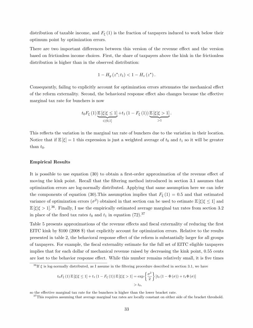
distribution of taxable income, and Fξ (1) is the fraction of taxpayers induced to work below their

optimum point by optimization errors.

There are two important differences between this version of the revenue effect and the version

based on frictionless income choices. First, the share of taxpayers above the kink in the frictionless

distribution is higher than in the observed distribution:

1−Hy (z?; t1) < 1−Hz (z?) .

Consequently, failing to explicitly account for optimization errors attenuates the mechanical effect

of the reform externality. Second, the behavioral response effect also changes because the effective

marginal tax rate for bunchers is now

t0Fξ (1)E [ξ|ξ ≤ 1]︸ ︷︷ ︸∈(0,1]

+t1 (1− Fξ (1))E [ξ|ξ > 1]︸ ︷︷ ︸>1

.

This reflects the variation in the marginal tax rate of bunchers due to the variation in their location.

Notice that if E [ξ] = 1 this expression is just a weighted average of t0 and t1 so it will be greater

than t0.

Empirical Results

It is possible to use equation (30) to obtain a first-order approximation of the revenue effect of

moving the kink point. Recall that the filtering method introduced in section 3.1 assumes that

optimization errors are log-normally distributed. Applying that same assumption here we can infer

the components of equation (30).This assumption implies that Fξ (1) = 0.5 and that estimated

variance of optimization errors (σ2) obtained in that section can be used to estimate E [ξ|ξ ≤ 1] and

E [ξ|ξ > 1].36. Finally, I use the empirically estimated average marginal tax rates from section 3.2

in place of the fixed tax rates t0 and t1 in equation (72).37

Table 5 presents approximations of the revenue effects and fiscal externality of reducing the first

EITC kink by $100 (2008 $) that explicitly account for optimization errors. Relative to the results

presented in table 2, the behavioral response effect of the reform is substantially larger for all groups

of taxpayers. For example, the fiscal externality estimate for the full set of EITC eligible taxpayers

implies that for each dollar of mechanical revenue raised by decreasing the kink point, 0.55 cents

are lost to the behavior response effect. While this number remains relatively small, it is five times

36If ξ is log-normally distributed, as I assume in the filtering procedure described in section 3.1, we have

t0Fξ (1)E [ξ|ξ ≤ 1] + t1 (1− Fξ (1))E [ξ|ξ > 1] = exp

{σ2

2

}[t0 (1− Φ (σ)) + t1Φ (σ)]

> t0,

so the effective marginal tax rate for the bunchers is higher than the lower bracket rate.37This requires assuming that average marginal tax rates are locally constant on either side of the bracket threshold.

33

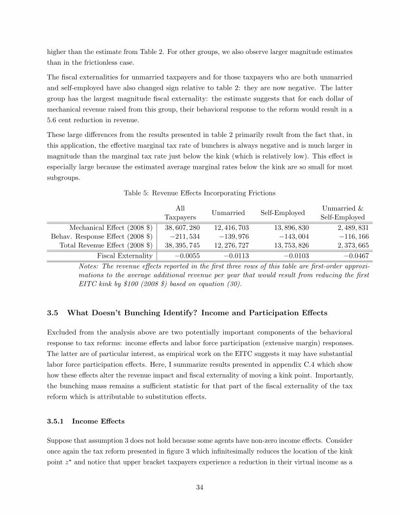
higher than the estimate from Table 2. For other groups, we also observe larger magnitude estimates

than in the frictionless case.

The fiscal externalities for unmarried taxpayers and for those taxpayers who are both unmarried

and self-employed have also changed sign relative to table 2: they are now negative. The latter

group has the largest magnitude fiscal externality: the estimate suggests that for each dollar of

mechanical revenue raised from this group, their behavioral response to the reform would result in a

5.6 cent reduction in revenue.

These large differences from the results presented in table 2 primarily result from the fact that, in

this application, the effective marginal tax rate of bunchers is always negative and is much larger in

magnitude than the marginal tax rate just below the kink (which is relatively low). This effect is

especially large because the estimated average marginal rates below the kink are so small for most

subgroups.

Table 5: Revenue Effects Incorporating Frictions

AllTaxpayers

Unmarried Self-EmployedUnmarried &Self-Employed

Mechanical Effect (2008 $) 38, 607, 280 12, 416, 703 13, 896, 830 2, 489, 831Behav. Response Effect (2008 $) −211, 534 −139, 976 −143, 004 −116, 166

Total Revenue Effect (2008 $) 38, 395, 745 12, 276, 727 13, 753, 826 2, 373, 665

Fiscal Externality −0.0055 −0.0113 −0.0103 −0.0467

Notes: The revenue effects reported in the first three rows of this table are first-order approxi-mations to the average additional revenue per year that would result from reducing the firstEITC kink by $100 (2008 $) based on equation (30).

3.5 What Doesn’t Bunching Identify? Income and Participation Effects

Excluded from the analysis above are two potentially important components of the behavioral

response to tax reforms: income effects and labor force participation (extensive margin) responses.

The latter are of particular interest, as empirical work on the EITC suggests it may have substantial

labor force participation effects. Here, I summarize results presented in appendix C.4 which show

how these effects alter the revenue impact and fiscal externality of moving a kink point. Importantly,

the bunching mass remains a sufficient statistic for that part of the fiscal externality of the tax

reform which is attributable to substitution effects.

3.5.1 Income Effects

Suppose that assumption 3 does not hold because some agents have non-zero income effects. Consider

once again the tax reform presented in figure 3 which infinitesimally reduces the location of the kink

point z? and notice that upper bracket taxpayers experience a reduction in their virtual income as a

34

result of the reform. If leisure is a normal good, these taxpayers should be expected to increase

their taxable income to partially offset this loss in income. Thus, moving the kink point changes the

mapping from the distribution of types into the distribution of taxable income under tax schedule

T1 and, consequently, changes the observed distribution of taxable income above the kink point.

3.5.2 Labor Force Participation Effects

Assumption 1 together with convexity of the tax schedule rules out extensive margin responses by

excluding the possibility that an agent’s indifference curve may be tangent to the budget constraint

at more than one point. One way to relax this assumption is to assume that agents face a fixed cost

of labor force participation and that they will only enter the labor force (i.e. have positive income)

if the gains from doing so exceed this cost. In this scenario, changes in the location of the kink

point can induce workers to enter or exit the labor force by changing the utility they receive if they

choose to work.

Returning to the tax reform presented in figure 3, there are two groups of taxpayers who experience

such participation effects. First, as noted above, a reduction in z? lowers the virtual income

associated with the upper tax bracket, decreasing the consumption of taxpayers who choose to enter

the labor force and locate in the upper bracket. For taxpayers at the margin of participating—those

whose fixed cost of work is exactly offset by the benefits of work—this reduced consumption will

induce them to exit the labor force. Second, recall that changing the location of a kink point has a

first-order effect on the utility of agents located at the kink (as I discussed in section 2.3). Again,

for taxpayers at the margin of participating, this will induce them to exit the labor force. Both

these types of participation effects cause a reduction in tax revenue.

3.5.3 Bringing It All Together

Although income and participation effects alters the revenue impact of moving a kink point, the

bunching mass still identifies the component of this impact attributable to the substitution effect.

In particular, the fiscal externality of moving a kink point becomes

FE (z?) = FEsub (z?) + FEinc (z?) + FEpart (z?) ,

where

FEsub (z?) ≡ − t0 (H1 (z?)−H0 (z?))

(t1 − t0) (1−H1 (z?))≤ 0,

is the part of fiscal externality caused by the substitution effects of the reform, and is identified by

the observed (pre-reform) distribution of taxable income. FEinc (z?) and FEpart (z?) are the parts

of the fiscal externality caused by income and participation effects (respectively). These terms are

defined in detail in Appendix C.4. Importantly, neither is identified by the observed distribution

35

of taxable income. Accounting for these effects in an ex ante evaluation of a proposed tax reform

requires relying on external evidence about the probable magnitude of these effects.

Other Extensive Margin Responses Participation effects are not the only extensive margin

responses that might be relevant to my analysis of the EITC. Small tax reforms can also cause

taxpayers to “jump” from one level of taxable income to another whenever the tax schedule induces a

non-convex budget set. Even under assumption 1, such non-convexity introduces the possibility that

taxpayer indifference curves can be tangent to the budget constraint at more than one point—that a

taxpayer may be at the margin between two distinct choices of positive income. We might therefore

be concerned that moving a convex kink in a tax schedule which also includes an non-convex kink

can potentially induce such taxpayers to jump from one income level to another. In principle, these

effects can be incorporated into the fiscal externality of the reform as I have done above with income

and participation effects, but I do not discuss this here. Bergstrom and Dodds (2021) provide an

extensive discussion of how these responses can affect optimal nonlinear income taxation.

3.5.4 Application to the EITC

The discussion above shows that the size of the bunching mass is informative about one component

of the behavioral response effect of moving the first EITC kink, but it may be important to account

for the other aspects of the behavioral response effect. Reducing the kink point might reduce revenue

due to taxpayers exiting the labor force at or above the kink point. Income effects would generate

an increase in revenue as some taxpayers increase their incomes. It is possible to supplement my

empirical analysis to account for these responses using income and participation elasticity estimates

derived from the literature. However, correctly accounting for the fiscal externality of participation

effects requires more detailed information about the change in total net government payments that

occurs when an individual above the kink moves to zero income. Such an analysis is complex and

beyond the scope of this paper.38

4 What is the Bunching Elasticity?

This section revisits standard bunching methodology in light of the results presented above. Bunching-

based elasticity estimates are closely connected to the behavioral response to moving a kink point,

but their application to other tax reforms of interest faces external validity challenges. In this

section, the conditions that give rise to these challenges are characterized analytically. Several

examples are presented which concretely demonstrate how particular behavioral assumptions can

compromise the external validity of the bunching elasticity.

38Bierbrauer, Boyer, and Hansen (2020) conduct an analysis of the efficiency consequences of the introduction ofthe EITC which accounts for these effects but confine their analysis to California due to the difficulty associated withconducting a full analysis.

36

4.1 Relating the Bunching Mass to Elasticities

Discussion of the standard bunching method requires a special case of the modeling framework that

I introduced in section 1.1. In particular, suppose that each agent’s type consists of a wage rate

w ∈ R++ and a vector of other characteristics ψ ∈ Ψ where Ψ is a convex (possibly multidimensional)

parameter space. That is to say, the agent’s type is θ = (w,ψ) and the type space is Θ = R++ ×Ψ.

For convenience, I will refer to a given value of ψ as a group.

Let F (w,ψ) represent the joint distribution of wages and group membership. For simplicity, I

maintain the assumption that there are no income effects (assumption 3) but the results below can

be easily extended to incorporate income effects. Thus, I can define z (t;w,ψ) as the taxable income

a type (w,ψ) agent chooses when facing a linear income tax rate t < 1 (irrespective of the intercept

of their budget constraint). Let H (z; t) be the distribution of taxable income under a tax rate of t,

as induced by the function z (t;w,ψ) and the parameter distribution F .

In addition to assumptions 1, 2, and 3, in this section I assume that within each group ψ agent

preferences satisfy the single-crossing condition with respect to the wage rate.

Assumption 4 (Single Crossing Condition). For all types (w,ψ) ∈ R++×Ψ and any tax rate t < 1,

taxable income is strictly increasing in the wage rate ∂z(t;w,ψ)∂w > 0.

With this additional assumption, it is possible to write the bunching mass as a function of compen-

sated elasticities of taxable income. Let

εc (t;w,ψ) ≡ −1− tz?

∂z (t;w,ψ)

∂t(31)

denote the compensated elasticity of taxable income for type (w,ψ) agents facing a linear tax rate

of t.

Theorem 5 (Bunching Mass in Terms of Elasticities). Under assumptions 1, 2, 3, and 4, and given

a piecewise linear tax schedule with two tax brackets (as defined in equation 2), the bunching mass

at the kink point can be written as:

H (z?; t1)−H (z?; t0) =

∫ t1

t0

εc (z?; t) · z?h (z?; t)

1− tdt, (32)

where εc (z?; t) is the average (compensated) elasticity of taxable income among agents who would

choose to locate at z? when facing a counterfactual linear tax schedule with a tax rate of t,

εc (z?; t) ≡ E [εc (t;w,ψ) |z (t;w,ψ) = z?] . (33)

37

Proof. The bunching mass at z? can be written as

H (z?; t1)−H (z?; t0) =

∫ψ

[H (z?|ψ; t1)− H (z?|ψ; t0)

]fψ (ψ) dψ

=

∫ψ

∫ t1

t0

∂H (z?|ψ; t)

∂tfψ (ψ) dψ

where the second equality follows from the fundamental theorem of calculus.

Note that the single crossing condition (assumption 4) ensures that for any linear tax rate t and

within any group ψ there exists a wage rate w? (t, ψ) at which group members would choose to locate

at the kink point. That is to say, there exists a function w? (t, ψ) satisfying z (t;w? (t, ψ) , ψ) = z? for

all t < 1 and ψ ∈ Ψ. Furthermore, the single crossing condition ensures that there is a straightforward

connection between the conditional distribution of taxable income and the conditional distribution

of wages:

H (z (t;w,ψ) |ψ; t) = F (w|ψ) .

Differentiating both sides of this expression with respect to t we obtain

∂H (z (t;w,ψ) |ψ; t)

∂t= −∂z (t;w,ψ)

∂th (z (t;w,ψ) |ψ; t)

and therefore the bunching mass can be expressed as

H (z?; t1)−H (z?; t0) = −∫ψ

∫ t1

t0

∂z (t;w? (t, ψ) , ψ)

∂th (z?|ψ; t) fψ (ψ) dtdψ

= −∫ t1

t0

{∫ψ

∂z (t;w? (t, ψ) , ψ)

∂t

h (z?|ψ; t) fψ (ψ)

h (z?; t)dψ

}h (z?; t) dt

The result then follows from using equation (31) to simplify the interior integral above.

Theorem 5 is simply a restatement of a result derived by Blomquist, Newey, Kumar, and Liang

(2019) and represents the most general formulation of the relationship between the bunching mass

and taxpayer elasticities. Importantly, equation (32) shows that the bunching mass is a function of

both agents’ elasticities and unobserved densities of taxable income. Thus, the bunching mass alone

cannot identify the ETI.

In order to obtain a weighted average of elasticities from an estimate of the bunching mass, it is

necessary to additionally an have an estimate of the normalization term

H ≡ z?∫ t1

t0

h (z?; t)

1− tdt. (34)

By dividing the bunching mass by H, it is possible to identify the bunching elasticity

εcB ≡∫ t1

t0

εc (z?; t) ρ (t) dt, (35)

38

which is a weighted average elasticity which places some positive weight

ρ (t) ≡h(z?;t)

1−t∫ t1t0

h(z?;t′)1−t′ dt′

, (36)

on the local average elasticity at the kink point under a linear tax rate t (εc (z?; t)) for each tax rate

t ∈ [t0, t1].

Corollary 3. Under assumptions 1, 2, 3 and 4, and given a piecewise linear tax schedule with

two tax brackets (as defined in equation 2), the bunching mass at the kink point together with the

normalizing term H identifies the bunching elasticity:

εcB =H (z?; t1)−H (z?; t0)

H(37)

Recent work in the bunching literature has called attention to the fact that the observed distribution

of taxable income cannot nonparametrically identify the bunching elasticity because it cannot

identify the normalization term H (Bertanha, McCallum, and Seegert, 2021; Blomquist, Newey,

Kumar, and Liang, 2019). Saez (2010) and Chetty, Friedman, Olsen, and Pistaferri (2011) proposed

identification strategies that relied on approximating H. Blomquist, Newey, Kumar, and Liang

(2019) and Bertanha, McCallum, and Seegert (2021) propose alternative approaches to obtaining

identification or partial identification of the bunching elasticity. These papers also show that

estimated elasticities can be quite sensitive to the choice of identification strategy. All these

identification strategies require imposing assumptions about how the density of taxable income

at z? (h (z?; t)) varies across different linear tax schedules, and in most cases further relies on the

assumption that agents have quasi-linear, isoelastic preferences and a constant elasticity.

Blomquist, Newey, Kumar, and Liang (2019) present a version of Corollary 3, and note that the

bunching elasticity (εcB) is subject to “issues of external validity” because it provides information

about a very specific convex combination of elasticities.39 In the next subsection, I build on their

work by more precisely characterizing these issues.

39It is important to note that this weighted average is not, in general, interpretable as the average elasticity ofbunchers. For example, in the special case where taxpayers have quasi-linear, isoelastic preferences it can be shownthat the bunching elasticity is the inverse of the expected inverse elasticity of the bunchers:

εcB =

(E[

1

εc|z1 (θ) < z? < z0 (θ)

])−1

.

Therefore, by Jensen’s inequality, this implies that the bunching elasticity is in fact strictly smaller than the averageelasticity of bunchers in this case.

39

4.2 Policy Analysis with the Bunching Elasticity

Corollary 1 already provides one unambiguously valid interpretation of the bunching elasticity.

Using equation (37), the fiscal externality of moving a kink point can be rewritten in terms of the

bunching elasticity:40

FE (z?) ≡ − t0t1 − t0

· H1−H1 (z?)

· εcB

However, Corollary 1 also makes it clear that decomposing the bunching mass into the bunching

elasticity (εcB) and the normalizing constant (H) is unnecessary for the purpose of identifying the

fiscal externality of moving a kink point. Thus, the value of such a decomposition depends on

whether the bunching elasticity is useful for analyzing other tax reforms of interest.

A natural candidate for a tax reform of interest is the effect of an infinitesimal change in the marginal

income tax rate either immediately below or immediately above the kink. In particular, consider a

tax schedule perturbation in the style of Saez (2001) which infinitesimally increases the marginal tax

rate just below z? and leaves it unchanged everywhere else. Applying results from the literature on

the perturbation approach to optimal nonlinear taxation, the fiscal externality of such a reform is41

FE−t (z?) ≡ − t01− t0

· z?h (z?; t0)

1−H (z?; t0)· εc (z?; t0) . (38)

Similarly, the fiscal externality of a tax reform which infinitesimally increases the marginal tax rate

just above z? is

FE+t (z?) ≡ − t1

1− t1· z?h (z?; t1)

1−H (z?; t1)· εc (z?; t1) . (39)

The fiscal externalities of these two local tax reforms can be estimated using the average elasticity

of two different types of “marginal bunchers”. In particular, FE−t (z?) depends on the average

elasticity of agents who would locate at the kink z? under the linear tax rate t0 (εc (z?; t0)), and

FE+t (z?) depends on the average elasticity of agents who would locate at the kink z? under the

linear tax rate t1 (εc (z?; t1)).

Precisely defining two local tax reforms of interest clarifies the elasticities needed to identify their

revenue consequences. This sheds light on two key issues: the external validity of the bunching

elasticity, and the differences between the revenue effects of moving a kink point and of infinitesimally

changing marginal rates near the kink point.

40Or, equivalently, the fiscal externality of increasing the tax rate just below the kink point from t0 to t1.41These results are usually framed in terms of welfare effects rather than fiscal externalities. The perturbation

approach to optimal taxation began with Saez (2001) and has subsequently been formalized and extended to the caseof multidimensional heterogeneity by Gerritsen (2016), Golosov, Tsyvinski, and Werquin (2014), and Jacquet andLehmann (2021). Bergstrom and Dodds (2021) extend these results to reforms of tax schedules which are almosteverywhere continuously differentiable (i.e. tax schedules that may contain kink points) so the expressions belowfollow from their results.

40

4.2.1 Determinants of External Validity

The definition of the bunching elasticity (equation 35) makes it clear that neither of the two

policy-relevant local average elasticities contained in equations (38) and (39) will generally be

identified by the standard bunching method. Although the bunching elasticity does assign positive

weight to both εc (z?; t0) and εc (z?; t1), in general, a given value of εcB is consistent with any finite,

positive values of εc (z?; t0) and εc (z?; t1). It is thus important to clarify under what circumstances

we should expect εcB to differ substantially from εc (z?; t0) and εc (z?; t1).

Equation (35) also makes it clear what the source of any such differences would be: endogeneity

of the local average ETI at the kink point (εc (z?; t)) to the tax rate. It can be shown that such

endogeneity results from two sources:42

dεc (z?; t)

dt= − 1

1− tCov (εc, (1 + α) εc|z = z?)︸ ︷︷ ︸

composition effect

+ E[∂εc

∂t|z = z?

]+ E

[(2− εc (z?; t)

εc

)∂εc

∂w

∂w? (t;ψ)

∂t|z = z?

]︸ ︷︷ ︸

misspecification effect

, (40)

where α (z; t, ψ) ≡ −(

1 + zh′(z|ψ;t)h(z|ψ;t)

)is the (second-order) Pareto parameter of the group-ψ-specific

distribution of taxable income at a given level of income z under tax rate t.43 Note that I have

suppressed the arguments of various functions in equation (40) for simplicity, and will continue to

do so below.44

To understand the first term in equation (40), note that, when agents exhibit multidimensional

heterogeneity (i.e. when there is more than one group ψ), changing the tax rate influences the

relative size of different groups among agents located at a given value of taxable income (in this

case, z?). This generates what Jacquet and Lehmann (2021) label a composition effect.45 We can

42See appendix C.5 for the derivation.43Note, for a continuous random variable X with distribution FX the function

xfX (x)

1− FX (x)

is sometimes described as the Pareto parameter at x in the public finance literature, because if FX has a Pareto tail,this measure converges to the Pareto parameter as x→∞. This claim is also true for the function

−(

1 +xf ′X (x)

fX (x)

),

and this measure has also sometimes been described in the public finance literature as the “Pareto parameter” (forexample, see Hendren (2020)). Because this paper includes references to both these measures, I distinguish the secondmeasure by labeling it as the second-order Pareto parameter at x.

44In particular, I have employed the convention that εc ≡ εc (t;w,ψ) and α ≡ α (z; t, ψ), and z ≡ z (t;w,ψ).45They discuss the implications of such effects for attempts to use sufficient statistics pertaining to an observed tax

system for the purpose of inferring the optimal tax system.

41

break composition effects down further:

Cov (εc, (1 + α) εc|z = z?) = (1 + E [α|z = z?]) Var (εc|z = z?)︸ ︷︷ ︸elasticity heterogeneity across groups

+ Cov (εc (εc − εc (z?; t)) , α|z = z?)︸ ︷︷ ︸heterogeneity of Pareto parameter across groups

(41)

The first term in this expression captures the fact that, all else equal, greater variance of elasticities

among agents at z? implies a larger magnitude composition effect. This variance effect is proportional

to the average group-specific Pareto parameter at z?. The second term is non-zero whenever group-

specific Pareto parameters are correlated with a particular function of group-specific elasticities.

Note that both of these types of composition effects are present if agents have isoelastic preferences

so that elasticities are constant within groups; it is variation in elasticities across groups that

generate composition effects.

The second term in equation (40) reflects another mechanism through which the tax rate can

influence the local average ETI εc (z?; t): if agent preferences are not isoelastic. I call this the

misspecification effect, in reference to the ubiquity of isoelastic function form assumptions in the

bunching literature (and in empirical public finance generally). As with the composition effect, the

misspecification effect can be broken down into two parts:

E[∂εc

∂t|z = z?

]︸ ︷︷ ︸

direct effect of tax rate

+E[(

2− εc (z?; t)

εc

)∂εc

∂w

∂w? (t;ψ)

∂t|z = z?

]︸ ︷︷ ︸

elasticity heterogeneity within groups

. (42)

The first term in this expression reflects the fact that when agents do not have isoelastic preferences,

the tax rate can directly influence the elasticity of taxable income. The second term will be present

whenever agents within the same group can have different elasticities (i.e. the group-specific elasticity

varies with the wage rate). The interpretation of this term is somewhat complex; intuitively, it

captures the fact that changes in the tax rate will generally change which members of a given group

choose to locate at a particular level of taxable income, and so if elasticities vary within groups such

changes can generate an indirect effect on the local average ETI. Note that both of these effects

would be present even in a model with unidimensional heterogeneity (i.e. if there were only one

group ψ).

To further clarify the nature of composition and misspecification effects, let us consider some

motivating examples.

Example 1 (Isoelastic Preferences with Constant Pareto Parameter). Suppose that all taxpayers

have quasi-linear, isoelastic preferences of the form

u (z;w,ψ) ≡ z − T (z)− w

1 + 1ψ

( zw

)1+ 1ψ,

so that

z (t;w,ψ) = w (1− t)ψ .

42

With this specification, agents within a given group all have the same elasticity: ψ. Thus, there are

no misspecification effects. Further suppose that all groups have wages are distributed according to

F , a distribution which is Pareto Type I above some threshold wage w0. That is to say, for any

w ≥ w0

Fw (w) = Fw (w0) + (1− Fw (w0))

(1−

(w

w0

)−a)for some Pareto slope parameter a > 1. Given these assumptions, it can be shown that for

any taxable income z > w0, all groups ψ will have the same group-specific Pareto parameter:

α (z; t, ψ) = a for all ψ and t < 1. This implies that the second term in equation (41) is zero. The

effect of the tax rate on the local average ETI can thus simply be written as

dεc (z?; t)

dt= − 1

1− t· (1 + a) ·Var (ψ|z = z?) .

Example 2 (Isoelastic Preferences with Non-Constant Pareto Parameter). Suppose that all tax-

payers have quasi-linear, isoelastic preferences but of a slightly different form than that discussed

above:

u (z;w,ψ) ≡ z − T (z)− 1

1 + 1ψ

( zw

)1+ 1ψ.

This specification implies a different taxable income function

z (t;w,ψ) = w1+ψ (1− t)ψ .

As in the previous example, within a given group all agents have the same ETI (ψ) and so there

are no misspecification effects. Again, suppose that wages are identically distributed across groups

according to F , a distribution which is Pareto Type I with slope a at any wage above w0. It can be

shown that for any taxable income z > w0, different groups have different local Pareto parameters.

In particular, α (z; t, ψ) = a1+ψ for all ψ and t < 1. This implies that the second term in equation

(41) is non-zero. The effect of the tax rate on the local average ETI can thus simply be written as

dεc (z?; t)

dt= − 1

1− t

[Var (ψ|z = z?) + aCov

(ψ,

ψ

1 + ψ|z = z?

)].

Example 3 (Unidimensional Heterogeneity with Multiple Incomes). Suppose that all taxpayers

have two sources of labor income (z1 and z2) and that their total taxable income is simply the sum

of these two incomes. For simplicity, I assume that both labor activities have the same wage rate.

Additionally, suppose that there is only one group ψ, so that agents differ only in their wage rate

w. Under this assumption, there are no composition effects but there is a misspecification effect.

Finally, suppose that agents have a separable utility function, with the disutility of income for each

source taking a quasi-linear, isoelastic form. In particular, suppose that an agent with wage rate w

43

chooses values of z1 and z2 to solve the problem

maxz1,z2>0

{z1 + z2 − T (z1 + z2)− w

1 + 1e1

(z1

w

)1+ 1e1 − w

1 + 1e2

(z2

w

)1+ 1e2

}.

Such an agent facing a linear tax rate t will choose to generate z1 (t;w) ≡ w (1− t)e1 dollars of

income from the first source and z2 (t;w) ≡ w (1− t)e2 dollars from the second source. Total taxable

income for such an agent is

z (t;w) ≡ z1 (t;w) + z2 (t;w)

= w [(1− t)e1 + (1− t)e2 ] .

Notice that the elasticities of z1 and z2 with respect to the net-of-tax rate are e1 and e2. These

elasticities are constant across all agents and across different tax rates. However, the elasticity of

taxable income is a convex combination of the elasticities of each of the two income sources

εc (t) ≡ z1 (t;w)

z (t;w)· e1 +

z2 (t;w)

z (t;w)· e2

=

((1− t)e1

(1− t)e1 + (1− t)e2

)e1 +

((1− t)e2

(1− t)e1 + (1− t)e2

)e2,

where the weights on the elasticity of each income source correspond to the share of the income

source in the agent’s total income. As shown above, these income shares are independent of taxpayer

wage rate, so the misspecification effect in this example is entirely a direct effect of taxation on this

elasticity. This direct effect stems from the fact that, as long as e1 6= e2, a change in the tax rate

changes the share of each type of income in total taxable income. Specifically, the misspecification

effect isdεc (t)

dt= −(e1 − e2)2

1− t· z1 (t;w)

z (t;w)· z2 (t;w)

z (t;w).

4.2.2 Infinitesimal Rate Changes vs. Moving Kinks

The external validity concerns associated with use of the bunching elasticity might seem unimportant

in light of the earlier results of this paper. As noted above, moving a kink point provides a mechanism

for implementing a specific local rate change. However, the impact of moving a kink point may differ

in important ways from the impact of other local tax reforms of interest. By comparing (38) and

(39) with the fiscal externality of moving a kink point, we can gain insight into these differences.

Inserting equation (32) into equation (20), we obtain an expression for the fiscal externality of

moving a kink point as a function of the average elasticity of taxable income at z? under various

44

counterfactual linear tax rates between t0 and t1:

FE (z?) = −t0∫ t1t0

z?h(z?;t)1−t εc (z?; t) dt

(t1 − t0) (1−H (z?; t1))(43)

This expression bears some superficial similarities in structure to the expressions describing the

fiscal externalities of the other local tax reforms introduced above (equations 38 and 39). To make

the connection more precise, we can rewrite FE (z?) in terms of the fiscal externalities of these

other local reforms. In each case, the fiscal externality of moving a kink point can be written as the

sum of a re-scaled version of the fiscal externality of the local tax reform and an adjustment term:

FE (z?) =

(1−H (z?; t0)

1−H (z?; t1)

)FE−t (z?)−

t0z?∫ t1t0

∫ tt0

{d

dt′

[h(z?;t′)

1−t′ εc (z?; t′)

]}dt′dt

(t1 − t0) (1−H (z?; t1)), (44)

and

FE (z?) =

(t0t1

)FE+

t (z?) +t0z

?∫ t1t0

∫ t1t

{d

dt′

[h(z?;t′)

1−t′ εc (z?; t′)

]}dt′dt

(t1 − t0) (1−H (z?; t1)). (45)

Note that the adjustment terms depend on how h(z?;t)1−t ε

c (z?; t) varies over the interval [t0, t1].

Evaluating the limits of equations (44) and (45) as t1 → t0, we can see that the fiscal externalities

of all three reforms converge for an arbitrarily small kink size. But for a finite sized kink, they will

differ from each other.

To better understand these differences, consider the adjustment terms in equations (44) and (45).

Note that the integrand in these terms can be decomposed into three effects:

d

dt

[h (z?; t)

1− tεc (z?; t)

]=h (z?; t)

(1− t)2

(εc (z?; t)− (1 + E [α|z = z?]) εc (z?; t)2

)︸ ︷︷ ︸

baseline effect

−h (z?; t)

(1− t)2

((1 + E [α|z = z?]) Var (εc|z = z?) + Cov

((εc)2 , α|z = z?

))︸ ︷︷ ︸

composition effect

+h (z?; t)

1− t

(E[∂εc

∂t|z = z?

]+ 2E

[∂εc

∂w

∂w? (t;ψ)

∂t|z = z?

])︸ ︷︷ ︸

misspecification effect

. (46)

As with equation (40) the composition effect in equation (46) is non-zero if there is heterogeneity

in agent elasticities across groups and the misspecification effect is non-zero if agent preferences

are non-isoelastic. Though these effects result from the same mechanisms as their counterparts in

equation (40) their precise nature differs somewhat. In addition, equation (46) includes a baseline

effect, which reflects that fact that even if taxpayers have isoelastic preferences and homogeneous

elasticities, h(z?;t)1−t remains endogenous to the tax rate.

If ddt

[h(z?;t)

1−t εc (z?; t)

]> 0 for all t ∈ [t0, t1], then equations (44) and (45) imply that the fiscal

45

externality of moving a kink point always falls between the fiscal externalities of the two local rate

changes:

0 > FE−t (z?) > FE (z?) > FE+t (z?) .

However, the sign of ddt

[h(z?;t)

1−t εc (z?; t)

]is ambiguous, so in principle it is possible that the fiscal

externality of moving a kink point FE (z?) could also be above or below both FE−t (z?) and

FE+t (z?).46This implies that there can exist Pareto- or welfare-improving movements of a kink

point even if such improvements cannot be obtained via infinitesimal local rate changes near the

kink point. On the other hand, the converse also holds true: in some cases, an infinitesimal local

rate change might be efficiency- or welfare-enhancing even when moving a kink point is not. Indeed,

this latter point holds irrespective of the sign of ddt

[h(z?;t)

1−t εc (z?; t)

].

4.3 Discussion

In comparing my proposed bunching methodology to the standard approach, two salient considera-

tions emerge. First, my method remains valid in the presence of multidimensional heterogeneity

and/or departures from isoelastic functional form assumptions, whereas the standard bunching

method—even in an ideal application where H is known—does not. Standard bunching estimates of

the ETI can thus generate misleading policy implications in circumstances where my method will

generate accurate policy implications. Second, policy analysis which focuses only on moving kink

points to the exclusion of other local tax reforms can miss on beneficial reform opportunities.

A strength of the new bunching method proposed in this paper is its robustness to any realization

of the unknown factors that determine how close a bunching-based elasticity (εcB) will be to the

policy-relevant local average elasticities εc (z?; t0) and εc (z?; t1). However, the same ambiguity about

these unknown factors also implies that it is impossible to know to what extent other beneficial local

tax reforms might be overlooked by a policy analysis that focuses exclusively on moving kink points.

Other Challenges to Bunching-Based ETI Estimation

While I have discussed the some of the major challenges to identification and interpretation of

bunching elasticities above, two further challenges are worth noting.

First, recall that bunching can be used to identify the revenue effect of moving a bracket threshold

even when tax schedules are heterogeneous across groups, as shown in section 3.2 of this paper. For

46To see that the sign of ddt

[h(z?;t)

1−t εc (z?; t)

]is ambiguous note because all three effects in equation (46) can be

positive or negative. The baseline effect is positive if and only if

εc (z?; t) <1

1 + E [α|z = z?].

The composition effect has an ambiguous sign because E [α|z = z?] can be above or below −1 and Cov((εc)2 , α|z = z?

)can be positive or negative. Finally, both components of the misspecification effect have ambiguous signs.

46

the purpose of bunching-based ETI estimation on the other hand, this heterogeneity presents another

challenge to the identification and interpretation of the bunching elasticity. In particular, note

that the definition of the bunching elasticity given in equation (35) has fixed bounds of integration

across taxpayers. While this expression can be extended to accommodate heterogeneous bounds

of integration, tax schedule heterogeneity is another limitation of bunching-based ETI estimation

methods that is relevant any time the data being used in the analysis pools taxpayers with differing

tax schedules together.

Second, Mortenson and Whitten (2020) show that in the case of the EITC, it appears that observed

bunching behavior is driven by taxpayers who simply report the level of income that maximizes

their tax refund. This refund-maximizing level of income often coincides with the first EITC kink

(or, in some years, other tax credit-induced kinks). They suggest that when this type of behavior

is driving observed bunching behavior, the bunching elasticity may be of limited policy-relevance.

Observed bunching in this case is primarily driven by the behavior of high (or even infinite) elasticity

taxpayers, whereas the population of taxpayers elsewhere will have much lower elasticities.

However, it should be noted that the use of bunching to analyze kink point movements is robust

to the presence of refund-maximizers. If a given kink point is the refund-maximizing point then

moving the kink results in refund-maximizing agents simply relocating to the new kink point. This

is precisely what the first-order approximation based on equation (11) assumes that all bunching

taxpayers will do after the reform, so this estimation method remains valid.

5 Conclusion

The concept of the elasticity of taxable income as a sufficient statistic for revenue and welfare

effects of taxation is powerful. However, as I show in this paper, it is not always necessary to have

an estimate of the ETI in order to predict the impact of a tax reform of interest. Under basic

theoretical restrictions, the bunching mass at a tax bracket threshold is itself a sufficient statistic

for the (compensated) behavioral response effect of local movements of the threshold. This use of

the bunching mass is fully nonparametric and requires no information about taxpayer preferences

beyond the observed distribution of taxable income generated by their choices.

Building on this result, I develop a new approach to revenue forecasting, as well as empirical tests for

Pareto efficiency and welfarist-optimality of piecewise linear tax schedules. An empirical application

to the EITC motivates extensions of these results that incorporate important features of real-world

policy settings. The results show that correctly incorporating optimization errors into revenue

analysis can have a meaningful impact on the estimated revenue effects of moving a tax bracket

threshold.

However, reforms that change bracket thresholds are not the only reforms of interest. Thus,

the method proposed in this paper is best viewed as a complement to—rather than a substitute

for—bunching-based elasticity estimation. By presenting a precise nonparametric interpretation

47

of the bunching mass, this paper clarifies the circumstances under which the bunching elasticity

provides a useful tool for predicting the behavioral response effect of other types of tax reforms. I

show that the discrepancy between the bunching elasticity and local policy-relevant elasticities near

the kink point depends on factors which are not currently well-documented empirically, such as the

variance of the ETI. Gathering evidence about these factors could therefore be of great value for

providing bunching practitioners with guidance on the external validity of their elasticity estimates.

Saez (2010) presented a tantalizing idea: that bunching in the observed distribution of taxable

income can teach us about the response to taxation even absent any variation in the tax schedule

over time or across different groups of taxpayers. Recent work has called this idea into question,

documenting substantial challenges to identification and interpretation. However, this paper shows

that by shifting our focus away from the ETI it is possible to deliver on the original promise of

bunching methodology by using the bunching mass to identify a different policy-relevant parameter

with a clear interpretation. The focus of prior bunching literature on the ETI makes sense given

the importance of this parameter in the broader public economics literature. However, this focus

has come at the cost of overlooking another valuable application of the bunching mass. Bunching

methodology may therefore offer a case study in the value of ensuring that policy-motivated empirical

work is tightly integrated with a formal welfare analysis of policy reforms of interest.

48

References

Apps, P., Van Long, N., & Rees, R. (2014). Optimal piecewise linear income taxation. Journal of

Public Economic Theory, 16 (4), 523–545.

Aronsson, T., Jenderny, K., & Lanot, G. (2018). The quality of the estimators of the ETI. Proceedings

of the Annual Conference on Taxation and Minutes of the Annual Meeting of the National

Tax Association, 111, 1–59.

Bergstrom, K., & Dodds, W. (2021). Optimal taxation with multiple dimensions of heterogeneity.

Journal of Public Economics, 200, 104442.

Bertanha, M., McCallum, A. H., & Seegert, N. (2021). Better bunching, nicer notching. arXiv

preprint arXiv:2101.01170.

Bierbrauer, F., Boyer, P., & Hansen, E. (2020). Pareto-improving tax reforms and the Earned

Income Tax Credit.

Blomquist, S., Newey, W. K., Kumar, A., & Liang, C.-Y. (2019). The bunching estimator cannot

identify the taxable income elasticity.

Cattaneo, M., Jansson, M., Ma, X., & Slemrod, J. (2018). Bunching Designs: Estimation and

Inference.

Chetty, R., Friedman, J. N., Olsen, T., & Pistaferri, L. (2011). Adjustment costs, firm responses, and

micro vs. macro labor supply elasticities: Evidence from Danish tax records. The Quarterly

Journal of Economics, 126 (2), 749–804.

Dong, Y., & Lewbel, A. (2015). Identifying the effect of changing the policy threshold in regression

discontinuity models. Review of Economics and Statistics, 97 (5), 1081–1092.

Feldstein, M. (1999). Tax avoidance and the deadweight loss of the income tax. Review of Economics

and Statistics, 81 (4), 674–680.

Gerritsen, A. (2016). Optimal nonlinear taxation: The dual approach.

Goff, L. (2021). Treatment Effects in Bunching Designs: The Impact of the Federal Overtime Rule

on Hours.

Golosov, M., Tsyvinski, A., & Werquin, N. (2014). A variational approach to the analysis of tax

systems.

Hahn, J., Todd, P., & Van der Klaauw, W. (2001). Identification and estimation of treatment effects

with a regression-discontinuity design. Econometrica, 69 (1), 201–209.

Hendren, N. (2020). Measuring economic efficiency using inverse-optimum weights. Journal of Public

Economics, 187, 104198.

Jacquet, L., & Lehmann, E. (2021). Optimal income taxation with composition effects. Journal of

the European Economic Association, 19 (2), 1299–1341.

Kleven, H. (2021). The eitc and the extensive margin: A reappraisal (Working Paper No. 26405).

National Bureau of Economic Research. https://doi.org/10.3386/w26405

Kopczuk, W. (2005). Tax bases, tax rates and the elasticity of reported income. Journal of Public

Economics, 89 (11-12), 2093–2119.

49

Kroft, K., Kucko, K., Lehmann, E., & Schmieder, J. (2020). Optimal income taxation with unem-

ployment and wage responses: A sufficient statistics approach. American Economic Journal:

Economic Policy, 12 (1), 254–92.

Kumar, A., & Liang, C.-Y. (2020). Estimating taxable income responses with elasticity heterogeneity.

Journal of Public Economics, 188, 104209.

Lewbel, A. (2019). The identification zoo: Meanings of identification in econometrics. Journal of

Economic Literature, 57 (4), 835–903.

Marx, B. M. (2018). The Cost of Requiring Charities to Report Financial Information.

Mortenson, J. A., & Whitten, A. (2020). Bunching to maximize tax credits: Evidence from kinks in

the us tax schedule. American Economic Journal: Economic Policy, 12 (3), 402–32.

Neisser, C. (2021). The Elasticity of Taxable Income: A Meta-Regression Analysis.

Saez, E. (2001). Using elasticities to derive optimal income tax rates. The Review of Economic

Studies, 68 (1), 205–229.

Saez, E. (2010). Do taxpayers bunch at kink points? American Economic Journal: Economic policy,

2 (3), 180–212.

Saez, E., Slemrod, J., & Giertz, S. H. (2012). The elasticity of taxable income with respect to

marginal tax rates: A critical review. Journal of Economic Literature, 50 (1), 3–50.

Sheshinski, E. (1989). Note on the shape of the optimum income tax schedule. Journal of Public

Economics, 40 (2), 201–215.

Slemrod, J., & Kopczuk, W. (2002). The optimal elasticity of taxable income. Journal of Public

Economics, 84 (1), 91–112.

Weber, C. E. (2014). Toward obtaining a consistent estimate of the elasticity of taxable income

using difference-in-differences. Journal of Public Economics, 117, 90–103.

Werning, I. (2007). Pareto Efficient Income Taxation.

50

A Discrete Kink Point Movements

The headline result of this paper pertains to infinitesimal movements of kink points. Since any

real-world tax reform is necessarily discrete in nature, it may be insightful to consider what can

(and cannot) be learned about the revenue effect of a discrete movement in a kink point using the

bunching mass. In particular, consider decrease in the location of the kink point from some initial

z? to some new point z?? < z?.

This reform has mechanical effects, which stem from the fact that any taxpayer initially located

above the kink point (z1 (θ) > z?) faces an increase in their tax liability of (t1 − t0)(z? − z??).Assuming there are no income effects, these agents will not change their choice of taxable income in

response to this reform, and therefore the mechanical effect of the reform on tax revenue is

(t1 − t0) (1−H1 (z?)) (z? − z??) . (47)

Turning to the behavioral response, as in the infinitesimal case we can split it into three components.

First, we have the relocation effect. Holding constant the size of the bunching mass, bunchers used

to pay t0z? in taxes, but now instead pay t0z

??, changing revenue by

− t0 (z? − z??) (H1 (z?)−H0 (z?)) , (48)

Adding (48) and (47) together we obtain the first-order approximation of the revenue effect of a

discrete change in the kink point (equation 11).

This approximation ignores the two additional components of the behavioral response: the new

buncher effect, and the former buncher effect. some taxpayers who previously located below the

kink will become bunchers. Specifically, those taxpayers whose choices under T0 and T1 satisfy,

z1 (θ) < z?? < z0 (θ) < z?.

The first-order approximation implicitly assumes these taxpayers continue to pay t0z0 (θ) in taxes,

but in reality, they now pay the lower amount t0z??. Thus, correcting the first-order approximation

to account for the new buncher effect reduces tax revenue by

− t0∫ z?

z??(z − z??)h0 (z) dz. (49)

On the other hand, some taxpayers who previously chose to bunch will stop bunching and locate

somewhere above the new kink point. These taxpayers are those whose choices under T0 and T1

satisfy

z?? < z1 (θ) < z? < z0 (θ) .

Approximating the behavioral response effect using the relocation effect implicitly assumes that

51

these taxpayers remain as bunchers but move to the new kink point, paying t0z?? in taxes. But

in fact, they pay the larger amount of t1 (z1 (θ)− z??) + t0z??. Thus, correcting the first-order

approximation for the former buncher effect increases tax revenue by

t1

∫ z?

z??(z − z??)h1 (z) dz. (50)

Adding (47), (48), (49), and (50) together we obtain the total effect of a discrete reform on tax

revenue:47

R (z??)−R (z?) = (t1 − t0) (z? − z??) (1−H1 (z?))︸ ︷︷ ︸mechanical effect

−t0 (z? − z??) (H1 (z?)−H0 (z?))︸ ︷︷ ︸relocation effect

(51)

− t0∫ z?

z??(z − z??)h0 (z) dz︸ ︷︷ ︸

new buncher correction

+ t1

∫ z?

z??(z − z??)h1 (z) dz︸ ︷︷ ︸

former buncher correction

Equation (51) provides some intuition for my main result. The bunching mass is a sufficient statistic

for the behavioral response to a small change in the location of the kink point because, for sufficiently

small reforms, the net impact of the new and former buncher effects is negligible.

Equation (51) presents the revenue effect of a discrete decrease in the location of a kink point. The

same equation can be used to describe the effect of increasing the location of a kink point from

z? to z?? > z?, but it is helpful to provide an explicit reinterpretation. The revenue effect of this

change can be written as

R (z??)−R (z?) = − (t1 − t0) (z?? − z?) (1−H1 (z?))︸ ︷︷ ︸first-order approximation of mechanical effect

+ t0 (z?? − z?) (H1 (z?)−H0 (z?))︸ ︷︷ ︸first-order approximation of behavioral response

(52)

· · · − t0∫ z??

z?(z?? − z)h0 (z) dz︸ ︷︷ ︸

former buncher correction

+ t1

∫ z??

z?(z?? − z)h1 (z) dz︸ ︷︷ ︸

new buncher correction

Recall, the first two terms in this expression provide a first-order approximation to the effect of

this reform. This approximation implicitly assumes that the revenue effect of the reform consists of

a reduction in the tax liability of all taxpayers initially located above the original kink point z?,

and an increase in revenue resulting from moving a fixed bunching mass to a higher locations. The

interpretation of errors this approximation introduces differs slightly from the case of a kink point

decrease however, where the approximation only introduced error into the behavioral response to

47The observant reader will notice that the derivation of equation (51) presented above abstracts from an additionalform of behavioral response to discretely decreasing a kink point: that some taxpayers will move from an interiorsolution in the lower tax bracket to an interior solution in the higher tax bracket. However, this is done only forexpositional simplicity; equation (51) can also be derived using the revenue function (8). The heuristic derivationworks because the new buncher effect accounts for the removal of these individuals from the lower bracket and theformer buncher effect accounts for their appearance in the higher bracket.

52

the reform. Here, it includes errors in both the behavioral response and the mechanical effect.

To see this, note that the first-order approximation implicit assumes that taxpayers initially located

in the upper tax bracket between the original kink point and the new kink point will continue to

choose z1 (θ) and will pay taxes of

t1 (z1 (θ)− z?) + t0z? − (t1 − t0) (z?? − z?)︸ ︷︷ ︸

mechanical effect

.

Instead, these individuals choose to become bunchers at the new kink point z??, paying taxes of

t0z??. The correction for this error take a simple form: the new buncher effect in equation (52).

There is also once again a former buncher effect, which corrects the error arising in the first-order

approximation due to the fact that some taxpayers exit the bunching mass after this reform. Following

an increase in the kink point, these taxpayers now locate somewhere on the lower tax bracket,

paying taxes of t0z0 (θ) rather than the t0z?? implicitly assumed when using the first-approximation

to the behavioral response to a reform.

Partial Identification and Approximations

Together, equations (51) and (52) provide a complete guide to the revenue effects of moving the

location of a kink point.

If the pre-reform distribution of taxable income is observed, it is easy to see that three out of the

four terms contained in equations (51) and (52) are identified. In both cases, the new buncher

effect is identified by the observed income distribution (in addition to two first-order approximation

terms). This is because the new buncher effect corrects for the first-order approximation’s implicit

assumption that they will continue to make the same choices that we currently observed them

making, when in fact they will end up at a known counterfactual bunching location z??.

By contrast, the former buncher effect is not identified by observed data, because it serves to correct

the first-order approximation’s implicit assumption that some taxpayers will locate at the new

bunching location z?? when in fact, they will end up choosing to locate some point on the new

budget constraint which is infeasible on the pre-reform budget constraint. As we don’t observe

these choices in pre-reform data, we cannot identify this effect. Notice, this non-identification result

stems from the same fundamental problem that underlies recent non-identification results regarding

the standard bunching method: counterfactual decisions of bunchers are not observed.48

While this is a valuable result in itself, it is possible to expand on the practical value of the result

by adopting a partial identification lens. For example, without any additional assumptions, we can

identify a lower bound on the revenue effect of a discrete decrease in the kink point by evaluating

48As I discuss in the previous section, this is what causes non-identification in the standard bunching method whenpreferences are quasi-linear and isoelastic, and the ETI is homogeneous. Outside this special case, knowledge ofcounterfactual decisions of bunchers is insufficient.

53

equation (51) with the former buncher effect set to zero. This works because, in the case of a

decrease in the kink point, the former buncher effect is always positive, so ignoring it will lead to an

underestimate of the effect. A similar result holds for the case of a discrete increase in the kink

point, but in this case evaluating equation (52) with the former buncher effect set to zero yields an

upper bound, because for such reforms the former buncher effect is always negative.

Rather than simply assuming the former buncher effect is zero, we could use a trapezoidal approxi-

mation to the former buncher effect. It turns out that such an approximation is identified by the

pre-reform distribution of taxable. In the case of a discrete decrease in a kink point we have

t1

∫ z?

z??(z − z??)h1 (z) dz ≈ (z? − z??)2

2t1h1 (z?) (53)

and in the case of a discrete increase we have

− t0∫ z??

z?(z?? − z)h0 (z) dz ≈ −(z? − z??)2

2t0h0 (z?) . (54)

Note, similar strategies have been employed in the traditional bunching literature from its inception.

Saez (2010) proposes the use of trapezoidal approximation for counterfactual distribution of income

for bunchers. However, in the standard bunching literature, identification of these approximations

themselves requires much stronger assumptions about agent behavior than those presented here,

because they include a counterfactual unobserved density. Equations (53) and (54) do not include

any such counterfactual densities because the error the former buncher effect is largest in the region

of taxable income close to the original kink point z?, but shrinks to zero close to the new kink point

z??.49

Imposing weak additional restrictions on the density of taxable income allows for a reinterpretation

of approximations (53) and (54) as bounds on the former buncher effect. In the case of a kink point

decrease, if h1 (z) is weakly decreasing for all z ∈ [z??, z?], then (53) provides a lower bound on

the former bunching effect. Conversely, if h0 (z) is weakly decreasing over this interval, then we

obtain an upper bound. Similarly, in the case of a kink point increase, if h0 (z) is weakly decreasing

(increasing) for all z ∈ [z?, z??], then (54) provides an upper (lower) bound on the former bunching

effect. Thus, when density functions are assumed to be monotone, sharper bounds on the revenue

effect of discrete changes are possible.

49Using higher derivatives of of the distribution of taxable income, it is possible to extend these approximationseven further. In fact, for any n ∈ N an nth-order Taylor approximation to the former buncher effect is identified bythe observed distribution, though the practical value of this extension is limited by the feasibility of estimating suchderivatives.

54

B Multiple Tax Brackets and Joint Reforms

My method can be easily extended to incorporate convex, piecewise linear tax schedules with more

than two brackets.50

Suppose the tax schedule is

T (z) ≡ maxi∈{0,1,...,n}

Ti (z) (55)

where for each i ∈ {0, 1, . . . , n} ,Ti (z) ≡ tiz − Vi. (56)

The tax schedule is thus fully characterized by a vector of bracket-specific marginal tax rates t =

(t0, t1, . . . , tn) and an accompanying vector of bracket-specific virtual incomes V = (V0, V1, . . . , Vn).

Suppose that (V, t) satisfies Vi > Vi−1 and ti > ti−1 for all i ∈ {1, 2, . . . , n}. Under these conditions,

equations (55) and (56) describe a convex, piecewise linear tax schedule.

Further suppose thatVi+1 − Viti+1 − ti

>Vi − Vi−1

ti − ti−1

for all i ∈ {1, 2, . . . , n− 1}. Then this tax schedule has n+ 1 different tax brackets and features n

different convex tax bracket thresholds (kink points) whose locations are implicitly defined by the

vectors of tax rates and virtual incomes (V, t). A taxpayer in the i-th bracket who is not bunching

at a kink point has income some income z ∈(Vi−Vi−1

ti−ti−1, Vi+1−Viti+1−ti

). The kink point z?i ≡

Vi+1−Viti+1−ti serves

as the the ith bracket and the (i+ 1)-th bracket.

As in section 1, the actual tax schedule is thus composed of many constituent linear tax schedules

of the form given by (56). Let zi (θ) be the choice of taxable income a type θ taxpayer would make

if they faced a particular linear tax Ti (z) and let H (z; ti) be the resulting distribution of taxable

income. Under assumptions 1 and 2, the corresponding density of taxable income under this linear

schedule (hi (z)) is continuous. Furthermore, we can describe the observed choices of taxpayers

under the piecewise linear tax schedule (55) as

z (θ) =

zi (θ) if zi (θ) ∈(z?i−1, z

?i

)z?i if zi+1 (θ) < z?i < zi (θ)

(57)

That is to say, if a taxpayer’s choice on a particular counterfactual linear tax schedule Ti (z) is

located in the tax bracket where the actual tax schedule (55) coincides with Ti (z), then the taxpayer

will choose an interior solution. On the other hand, the taxpayer will locate at a given kink point

50Indeed, it can actually be extended to include any budget set formed by the intersection of some finite setof smooth, convex budget sets. That is to say, the tax schedule within each tax bracket can be nonlinear, aslong as it is convex and continuously differentiable. Thus, for example, my method could be readily be ap-plied to analyze any bunching observed at the first kink point in the German income tax schedule, where themarginal tax rate rises discontinuously from 0 to 14% and thereafter increases continuously until reaching 42%(https://taxsummaries.pwc.com/germany/individual/taxes-on-personal-income). Such an extension is straightforward,and for simplicity I will focus here on only the piecewise linear case.

55

z?i which divides the i-th and (i+ 1)-th tax brackets if their choice under the counterfactual linear

tax schedule Ti (z) is located above the kink point and their choice under Ti+1 (z) is located below

the kink point. By the strong axiom of revealed preference, all taxpayers will satisfy one and only

one of these possible conditions.51

It follows from equation (5), that the observed distribution of taxable income will be

H (z) =

H (z; ti) if z ∈(z?i−1, z

?i

)H (z?i ; ti+1)−H (z?i ; ti) if z = z?i

(58)

Tax revenue under the tax schedule (55) can be written as a

R (z?) ≡n∑i=0

(∫ z?i

z?i−1

Ti (z)h (z; ti) dz

)+

n∑i=1

tiz?i (H (z?i ; ti+1)−H (z?i ; ti)) (59)

where Ti (z; z?) refers to the counterfactual linear tax schedules of equation (56). I have adjusted

the notation here to make clear that, in general, the virtual income for each of these counterfactual

tax schedules depends on multiple kink point locations. Note as well, that for equation 59 to provide

a full description of tax revenue requires adopting the convention that V−1 = V0 so that z?−1 = 0.

If we continue to rule out income effects (assumption 3), the first-order revenue effect of equally

decreasing the virtual income level for tax brackets with an index j > i is

− ∂R (z?)

∂κ= 1−H (z?i ; ti+1)− ti

ti+1 − ti(H (z?i ; ti+1)−H (z?i ; ti)) . (60)

But notice, this expression is proportional to the first revenue effect of decreasing a kink because

that is exactly what such a reform does: it moves the kink point by adjust virtual income lev-

els/Consequently the first-order welfare effects are also the same. Thus, Theorems 1–4 continue to

apply in the case of multiple tax brackets. The fiscal externality of decreasing all Vj for j > i is

FE (z?i ) ≡ − ti (H (z?i ; ti+1)−H (z?i ; ti))

(ti+1 − ti) (1−H (z?i ; ti+1)). (61)

51That at least one such condition must hold follows from the fact that the agent must choose some location on thebudget set. To see why only one condition can hold, note that the budget set induced by the actual tax schedule (55)is simply the intersection of the budget sets induced by our n+ 1 counterfactual linear tax schedules. This means thatif for some type θ we have zi (θ) ∈ (z?i , z

?i+1) and zj (θ) ∈

(z?j , z

?j+1

)for i 6= j, then zi (θ) � zj (θ) by SARP because

zj (θ) is affordable under the linear schedule Ti. Similarly, zj (θ) � zi (θ) because zi (θ) is affordable under the linearschedule Tj , a contradiction. Similarly, suppose that for type θ, zi+1 (θ) < z?i+1 < zi (θ) and zj+1 (θ) < z?j+1 < zj (θ)for some i 6= j. Suppose, without loss of generality, that i > j. This implies that zi (θ) is affordable under Tj+1 andthat zj+1 (θ) is affordable under Ti. Thus, by SARP, we have zi (θ) � zj+1 (θ) and zj+1 (θ) � zi (θ). Similar reasoningcompletes the proof.

56

B.1 Moving Two Kinks

Suppose instead of moving a full set of virtual incomes we only alter decrease the virtual income Vi

in the ith bracket. Such a reform has the effect of implicitly changing the location of both kink

points that border the bracket, decreasing the lower kink point (z?i−1) and increasing the upper

kink point (z?i ). By considering this reform, we can develop tests of Pareto efficiency and welfarist

optimality that go beyond the tests developed in section 1.

Consider a tax reform, indexed by κ ∈ R, that simultaneously moves the locations of two kinks

points z?i and z?j , satisfying z?j > z?i . In particular, the reform decreases the location of z?i and

increases the location of z?j as follows

∂z?i∂κ

= −1∂z?j∂κ

=ti − ti−1

tj − tj−1, (62)

while leaving the locations of all other kink points constant. Notice, independently decreasing the

location of the lower kink point z?i would result in a mechanical effect that collects additional revenue

from all taxpayers above this kink. But by increasing the location of the higher kink point z?j in

just the right proportion, this joint reform offsets this effect for any taxpayers above z?j , keeping the

mechanical effect confined to only those taxpayers between the two kink points under consideration

(z?i and z?j ).

Thus, absent income effects, the first-order effect of this reform on tax revenue is

−dR (z?)

dVi= H (z?i ; ti)−H

(z?i−1; ti

)︸ ︷︷ ︸mechanical effect

(63)

−(

ti−1

ti − ti−1

) bunching mass at z?j︷ ︸︸ ︷(H(z?i−1; ti

)−H

(z?i−1; ti−1

))+

titi+1 − ti

bunching mass at z?i︷ ︸︸ ︷(H (z?i ; ti+1)−H (z?i ; ti))︸ ︷︷ ︸

revenue effect of behavioral response

.

As with single kink point reforms, this effect is identified from the observed distribution of taxable

income, though it now requires using the size of two bunching masses (one for each kink point).

However, this joint reform differs from single kink reforms in a key respect: the behavioral response

consists of both a positive and negative component. On the one hand, the reform decreases taxable

income for the bunchers at the lower kink point, a behavioral response that decreases tax revenue.

On the other hand, the reform increases taxable income for bunchers at the higher kink point, a

behavioral response that increases tax revenue.

The fiscal externality of this tax reform is

FEVi ≡ −ti−1

ti−ti−1

(H(z?i−1; ti

)−H

(z?i−1; ti−1

))− ti

ti+1−ti (H (z?i ; ti+1)−H (z?i ; ti))(H (z?i ; ti)−H

(z?i−1; ti

)) . (64)

57

We can re-write this as a function of the fiscal externalities of decreasing the two kink points by

themselves (using equation 61):

FEVi =

(1−H

(z?i−1; ti

)H (z?i ; ti)−H

(z?i−1; ti

))FE (z?i )−

(1−H (z?i ; ti+1)

H (z?i ; ti)−H(z?i−1; ti

))FE (z?i+1

). (65)

This expression makes it clear that, in principle, it is possible for the fiscal externality of this type

of joint reform to be positive.

Theorem 6 (Test for Pareto Efficiency (Multibracket)). Under assumptions 1, 2, and 3, then a

piecewise linear tax schedule which is Pareto efficient must satisfy

FE (z?i ) ≥ −1 (66)

for every kink point z?i , and

FEVi ≥ −1 (67)

for every virtual income level Vi.

Moreover, when a tax schedule satisfies both of these conditions (and the relevant second-order

conditions in edge cases where FE (z?i ) = −1 or FEVi = −1) no Pareto-improvement can be obtained

through any infinitesimal tax reform that jointly moves any set of kink points.

The second part of this theorem is analogous to the result presented in Bierbrauer, Boyer, and

Hansen (2020), which shows that if there are no Pareto-improving “single-bracket” or “two-bracket”

reforms to marginal tax rates, then there are no Pareto-improving reforms.52 Theorem 6 states that

if the are no Pareto-improving moves of a single kink point, and no Pareto-improving joint reforms

of the kind described above, then there are no other Pareto-improvements which can be obtained

through jointly moving kink points (infinitesimally).

Sketch of a proof: This result can be derived by first demonstrating that the fiscal externality of any

joint movement of a collection of kink points can be written as a linear combination of the fiscal

externalities of moving individual kink points (as equation 65 does for the particular joint reform

discussed above). It is not difficult to then show that any the existence of a Pareto-improving joint

movement of three kink points would imply that either condition 66 or condition 67 must fail.

52Note, in Bierbrauer, Boyer, and Hansen (2020), “single-bracket” and “two-bracket” reforms do not refer to changesin tax rates within different tax brackets in a piecewise linear tax schedule but rather describe local reforms at a singlepoint in the tax schedule which can be intuitively described as “single-bracket” and “two-bracket”.

58

C Derivations

C.1 Alternative Heuristic Derivation of Theorem

Here I present an alternative approach to building intuition for the result in Theorem 1, one based

on showing that the errors that result from using equation (11) to approximate revenue effects are

second-order.

Consider a tax reform which infinitesimally lowers the kink point by dz? (moving it from z?

to z? − dz?). This reform discretely increases the marginal tax rate within a small window of

taxable income immediately below z? while simultaneously reducing the demogrant (virtual income)

associated with the second tax bracket.

A seemingly naive approximation of the effect of this reform consists of summing together the

following two components:

1. The approximate mechanical effect is the additional tax revenue generated by taxpayers with

incomes in the upper bracket before the reform. Such agents pay a higher marginal rate on

their earnings in the interval (z? − dz?, z?], so that each such agent’s tax liability increases by

by (t1 − t0) dz?. This group of agents has a mass of 1−H1 (z?), resulting in a total revenue

effect of

(t1 − t0) (1−H1 (z?)) dz?.

2. The relocation effect is the loss in tax revenue that results from simply moving all bunchers

from z? to z? − dz?, holding constant the size of the bunching mass. For each such agent, tax

liability falls by −t0dz?. These agents a pre-reform mass of H1 (z?)−H0 (z?), resulting in a

total revenue effect of:

−t0 (H1 (z?)−H0 (z?)) dz?.

Note, in contrast to the assumptions of the relocation effect, the size of the bunching mass will not in

fact remain constant because some agents are at at the margin between bunching and not bunching

pre-reform. For example, the group of agents with z0 (θ) ∈ (z? − dz?, z?) are initially in the lower

tax bracket but after the tax reform, these agents will become bunchers. As a result their taxable

income will fall from z0 (θ) to z?− dz?, inducing a reduction in tax revenue by t0 (z0 (θ)− z? + dz?).

For the case of an infinitesimal kink point shift, the mass of these agents is h0 (z?) dz? and their

pre-reform taxable income is z0 (θ) = z?. Thus, we can account for this additional loss in revenue

by adding the new buncher correction,

−t0h0 (z?) (dz?)2 ,

to our naive approximation.

59

There is also be a group of agents with z1 (θ) ∈ (z? − dz?, z?) who are bunching in the pre-reform

period but will leave the bunching mass after the reform, choosing a post-reform level of taxable

income z1 (θ), in the upper tax bracket. The relocation effect implicitly assigns these taxpayers a

post-reform income of z? − dz?, underestimating the post-reform tax revenue they will generate

by t1 (z1 (θ)− z? + dz?). For the case of an infinitesimal kink point shift, the mass of these agents

is h1 (z?) dz? and their post-reform taxable income is z1 (θ) = z?. Thus, we can account for this

additional gain in revenue by adding the former buncher correction,

t1h1 (z?) (dz?)2 ,

to our naive approximation.

Theorem 1 follows from the fact that these new and former buncher corrections are both second-

order.53

C.2 Heterogeneous Tax Rates

Suppose that type θ agents face the following two bracket tax schedule

T (z; θ) ≡

t0 (θ) z if z ≤ z? (θ)

t1 (θ) z + [t0 (θ)− t1 (θ)] z? (θ) if z > z? (θ),

where z? (θ), t0 (θ), and t1 (θ) are type-θ-specific tax schedule parameters. Let tax revenue from a

type θ taxpayer be denoted as

T (θ) ≡ T (z (θ) ; θ) .

Total tax revenue can then be written as

R ≡∫T (θ) f (θ) dθ.

Now consider a tax reform indexed by κ which infinitesimally changes the location of the kink point

for type θ taxpayers by dz?(θ)dκ . The revenue effect of this reform is

dR

dκ=

∫dT (θ)

dz? (θ)

dz? (θ)

dκf (θ) dθ

where

dT (θ)

dz? (θ)≡

0 if z0 (θ) ≤ z? (θ)

t0 (θ) if z1 (θ) < z? (θ) < z0 (θ)

t0 (θ)− t1 (θ) if z1 (θ) ≥ z? (θ)

.

53That is, as dz? → 0, an effect which is proportional to(dz?)2 shrinks faster than an effect which is proportional todz?.

60

As in the standard case, some taxpayers are below the kink, and face no change in tax payments,

some are above the kink and face a mechanical change in tax payments, and some are (non-marginal)

bunchers and face a change in tax payments due to their behavioral response.The difference is that

now the kink point locations and marginal rates are variable across individuals. For a general reform

we havedR

dκ=

∫θ∈Θ1

[t1 (θ)− t0 (θ)]dz? (θ)

dκf (θ) dθ −

∫θ∈ΘB

t0 (θ)dz? (θ)

dκf (θ) dθ (68)

where Pr {z1 (θ) < z? (θ) < z0 (θ)} is the generalized bunching mass—the fraction of taxpayers who

are bunching at their own kink point—and Pr {z1 (θ) > z? (θ)} is the fraction of taxpayers who are

located above their own kink point.

In the main text, I assume that all taxpayers have the same kink point location so that z (θ) = z?

for all θ so that

Pr {z1 (θ) < z? (θ) < z0 (θ)} = H1 (z?)−H0 (z?)

and Pr {z1 (θ) > z? (θ)} = 1 −H1 (z?). Letting dz?(θ)dκ = −1, equation (68) simplifies to equation

(29).

C.3 Frictions

Suppose that the observed value of taxable income reflects a combination of the taxpayer’s optimal

choice and a random optimization error. In particular, let observed taxable income for a type θ

agent be

z (θ, ξ) = y (θ) ξ

where y (θ) is the optimal choice of income for this taxpayer and ξ ∼ Fξ is a multiplicative

optimization error. I assume these errors are iid, and that the support of Fξ is a convex subset of

R++.54 Suppose that assumptions 1—3 hold. Let Hy (·; t) be the distribution of taxpayer optimal

choices under a linear tax schedule with marginal tax rate t < 1, and let hy (·; t) be the corresponding

density of optimal choices.

Total tax revenue derived from this tax system is

R (z?) ≡∫ z?

0R (y; z?)hy (y; t0) dy+R (z?; z?) (Hy (z?; t1)−Hy (z?; t0))+

∫ ∞z?

R (y; z?)hy (y; t1) dy

(69)

where

R (y; z?) ≡ t0∫ z?/y

0yξfξ (ξ) dξ +

∫ ∞z?/y

[t1 (yξ − z?) + t0z?] fξ (ξ) dξ (70)

is the average tax revenue generated by taxpayers with an optimal income of y. Note, the revenue

54This allows for the possibility of a bounded or unbounded error distribution and ensures that z (θ, ξ) > 0 ⇐⇒y (θ) > 0.

61

function without frictions (equation 8) can be obtained as a special case of equation (69) when Fξ is

a degenerate distribution such that P {ξ = 1} = 1.

The derivative of equation (69) can be written as

R′ (z?) = R (z?; z?)hy (z?; t0) + R (z?; z?) (hy (z?; t1)− hy (z?; t0))− R (z?; z?)hy (z?; t1)︸ ︷︷ ︸=0 (new and former buncher effects)

+

∫ z?

0

∂R (y; z?)

∂z?hy (y; t0) dy +

∫ ∞z?

∂R (y; z?)

∂z?hy (y; t1) dy

+

∂R (y; z?)

∂y

∣∣∣∣∣y=z?

+∂R (z?; z?)

∂z?

(Hy (z?; t1)−Hy (z?; t0)) (71)

Note that, as in the frictionless case, terms which are related to the new and former buncher effects

cancel out. This is a consequence of the fact that changing the kink point induces the same changes

in taxpayer optimal choices as in the frictionless case. The difference in revenue effect in stems

from the fact that taxpayer optimal choices are differently aggregated into changes in revenue when

optimization errors are present.

To further simplify equation (71), we can substitute in expressions for ∂R(y;z?)∂z? and ∂R(y;z?)

∂y

∣∣∣y=z?

.

The former partial derivative captures changes average revenue from a taxpayer who chooses optimal

income y as a result of changing the kink point:

∂R (y; z?)

∂z?= − (t1 − t0)

(1− Fξ

(z?

y

)).

Following an increase of the kink point, all such taxpayers will pay slightly less in taxes any time

they taxable income falls above z?, due to the mechanical effect of the reform. The second partial

derivative we need captures the behavioral response effect caused by the change in the optimal

choice of bunchers:55

∂R (y; z?)

∂y

∣∣∣∣∣y=z?

= t0

∫ 1

0ξfξ (ξ) dξ + t1

∫ ∞1

ξfξ (ξ) dξ

= t0Fξ (1)E [ξ|ξ ≤ 1] + t1 (1− Fξ (1))E [ξ|ξ > 1] .

55Here, we define bunchers as taxpayers whose optimal choice is to locate at the kink (y (θ) = z?) even though theymay not locate at the kink due to optimization error.

62

Substituting these into equation (71) and applying integration by parts we get

R′ (z?) = − (t1 − t0) (1−Hz (z?; z?))︸ ︷︷ ︸mechanical effect

+ (t0Fξ (1)E [ξ|ξ ≤ 1] + t1 (1− Fξ (1))E [ξ|ξ > 1]) (Hy (z?; t1)−Hy (z?; t0))︸ ︷︷ ︸behavioral response effect

.

The fiscal externality of moving a kink in this model can be written as

FE (z?) = −(t0Fξ (1)E [ξ|ξ ≤ 1] + t1 (1− Fξ (1))E [ξ|ξ > 1]

t1 − t0

)(Hy (z?; t1)−Hy (z?; t0)

1−Hz (z?; z?)

). (72)

The second-order revenue effect is

R′′ (z?) = (t1 − t0)dHz (z?; z?)

dz?

+ (t0Fξ (1)E [ξ|ξ ≤ 1] + t1 (1− Fξ (1))E [ξ|ξ > 1]) (hy (z?; t1)− hy (z?; t0))

where

dHz (z?; z?)

dz?=∂Hz (z; z?)

∂z

∣∣∣∣z=z?

+∂Hz (z; z?)

∂z?

∣∣∣∣z=z?

=

∫ 1

0hy (z?ξ; t0) fξ (ξ) dξ +

∫ ∞1

hy (z?ξ; t1) fξ (ξ) dξ,

because

Hz (z; z?) ≡∫ z?/z

0Hy (zξ; t0) fξ (ξ) dξ +

∫ ∞z?/z

Hy (zξ; t1) fξ (ξ) dξ,

∂Hz (z; z?)

∂z

∣∣∣∣z=z?

=

∫ 1

0hy (z?ξ; t0) fξ (ξ) dξ+

∫ ∞1

hy (z?ξ; t1) fξ (ξ) dξ+1

z?fξ (1) [Hy (z?; t1)−Hy (z?; t0)] ,

and∂Hz (z; z?)

∂z?

∣∣∣∣z=z?

= − 1

z?fξ (1) (Hy (z?; t1)−Hy (z?; t0)) .

C.4 Income and Participation Effects

Suppose that taxpayers face the two-bracket tax schedule (2). For each type of taxpayer θ, I assume

that they make two choices:

1. Whether or not to enter the labor force.

2. Conditional on entering the labor force, how much income to earn.

Allowing for the possibility of income effects, a type θ taxpayer who enters the labor force will

choose a value of taxable income that solves the problem utility maximization (1) where their utility

63

function is assumed to satisfy Assumption 1. Recall, z (t, V ; θ) is the choice of taxable income a

type θ agent would make if facing a linear tax schedule with marginal tax rate t and virtual income

V . Conditional on entering the labor force, the choice of taxable income a type θ agent makes when

facing the kinked tax schedule (2) can be written as

z (θ) =

z (t0, V0; θ) if z (t0, V0; θ) < z?

z (t1, V1; θ) if z (t1, V1; θ) > z?

z? if z (t1, V1; θ) ≤ z? ≤ z (t0, V0; θ)

,

where V0 ≡ G and V1 ≡ (t1 − t0) z? +G. As in section (1.1), it remains that case that all taxpayers

must satisfy one, and only one of the three conditions in equation listed above. The alternative

possibility (z (t0; θ) < z? < z (t1; θ)) would violate SARP, since the z (t0; θ) would be affordable

under T1 and z (t1; θ) would be affordable under T0.

Let vE (θ) be the indirect utility associated with a type θ agent’s utility maximization problem:

vE (θ) ≡ u (z (θ)− T (z (θ)) , z (θ) ; θ) .

On the other hand, let vU (θ) be the utility a type θ agent would receive if unemployed:

vU (θ) ≡ u (T (0) , 0; θ) .

I assume that a type θ taxpayer only chooses to enter the labor force if the private benefit of

doing so exceeds some fixed cost of work ξ. Assuming that ξ ∼ Q (·|θ) for all type θ taxpayers, the

probability that such a taxpayer enters the labor force is

Q (θ) ≡ Q (vE (θ)− vU (θ) |θ) .

Total tax revenue in this economy can constructed by integrating over the type distribution:

R (z?) ≡ t0∫θ∈Θ0(z?)

z (t0, V0; θ)Q (θ) f (θ) dθ︸ ︷︷ ︸lower bracket revenue

+ t0z?

∫θ∈ΘB(z?)

Q (θ) f (θ) dθ︸ ︷︷ ︸buncher revenue

+

∫θ∈Θ1(z?)

[t1 (z (t1, V1; θ)− z?) + t0z?]Q (θ) f (θ) dθ︸ ︷︷ ︸

upper bracket revenue

(73)

where

Θ0 (z?) = {θ ∈ Θ : z (t0, V0; θ) < z?}

is the set of types who choose to locate at an interior point the lower tax bracket if they enter the

64

labor force,

Θ1 (z?) = {θ ∈ Θ : z (t1, V1; θ) > z?}

is the set of types who choose to locate in the upper tax bracket if they enter the labor force, and

ΘB (z?) = {θ ∈ Θ : z (t1, V1; θ) ≤ z? ≤ z (t0, V0; θ)}

is the set of types who choose to bunch if they enter the labor force.

Differentiating equation (73), and applying the multidimensional version of Leibniz rule, we obtain

−R′ (z?) = (t1 − t0)

∫θ∈Θ1

Q (θ) f (θ) dθ︸ ︷︷ ︸mechanical effect

−t0∫θ∈ΘB

Q (θ) f (θ) dθ︸ ︷︷ ︸substitution effect

−t1 (t1 − t0)

∫θ∈Θ1

∂z (t1, V1; θ)

∂V1Q (θ) f (θ) dθ︸ ︷︷ ︸

income effect

−t0z?∫θ∈ΘB

(1− t0 −MRS (z?, θ))∂u (θ)

∂cq (θ) f (θ) dθ︸ ︷︷ ︸

participation effect (bunchers)

−∫θ∈Θ1

[t1 (z (t1, V1; θ)− z?) + t0z?] (t1 − t0)

∂u (θ)

∂cq (θ) f (θ) dθ︸ ︷︷ ︸

participation effect (upper bracket taxpayers)

(74)

where q (θ) ≡ Q′ (vE (θ)− vU (θ) |θ) is the density of the fixed cost of working for type θ agents

evaluated at vE (θ)− vU (θ).

The first two terms in equation (74) are familiar from the discussion in section (1.2): the mechanical

effect of the reform and the relocation effect. The income effect captures the revenue consequences

of the behavioral responses of taxpayers located above the kink point who may choose to respond to

their loss of income by increasing their earnings. For an infinitesimal reduction in the location of the

kink point, these taxpayers experienced an income loss of t1 − t0, and their response is proportional

to the size of this loss. If leisure is a normal good then ∂z(t1,V1;θ)∂V1

≤ 0 for all types θ, so this effect

will be positive as long as t1 > 0.

The participation effects capture the fact that some taxpayers will choose to exit the labor force

after the reform. Specifically, these are taxpayers who were at the margin between participating and

not participating before the reform. Because the utility these agents derive from working declines

following the reform, they will no longer choose to do so. For bunchers, the resulting change in the

participation rate is proportional to the first-order reduction in utility caused by their behavioral

response to the reform (as discussed in section (2.3)). For upper bracket taxpayers, the resulting

change in the participation rate is proportional to the utility loss they experience due to their

reduction in virtual income.

65

Let

π (θ) ≡ 1

Q (θ)

∂u (θ)

∂cq (θ)

be the semi-elasticity of labor force participation rate of type θ agents with respect to their

consumption c (θ) and let

η (θ) ≡ −∂z1 (θz (t1, V1; θ))

∂V1≥ 0

be the magnitude of the income effect for type θ agents (conditional on labor force participation).

We can rewrite equation (74) as

−R′ (z?) = (t1 − t0) (1−H1 (z?))︸ ︷︷ ︸mechanical effect

−t0 (H1 (z?)−H0 (z?))︸ ︷︷ ︸substitution effect

+ t1 (t1 − t0) (1−H1 (z?)) η+ (z?)︸ ︷︷ ︸income effect

−t0z? (H1 (z?)−H0 (z?))E [k (θ)π (θ) |z (θ) = z?]︸ ︷︷ ︸participation effect (bunchers)

−t1 (t1 − t0) (1−H1 (z?))E [(t1 (z (θ)− z?) + t0z?)π (θ) |z (θ) > z?]︸ ︷︷ ︸

participation effect (upper bracket taxpayers)

(75)

where

η+ (z?) ≡ E [η (θ) |z (θ) > z?]

is the average income effect of the kink point and

k (θ) ≡ 1− t0 −MRS (z?, θ) .

The total fiscal externality of moving the kink point is

FE (z?) = FEsub (z?) + FEinc (z?) + FEpart (z?) ,

where the portion attributable to the substitution effect is

FEsub (z?) ≡ − t0 (H1 (z?)−H0 (z?))

(t1 − t0) (1−H1 (z?))≤ 0.

The parts of FE (z?) associated with the income and participation effects can be obtain by normal-

izing these effects (as they appear in equation (75)) by the mechanical effect:

FEinc (z?) ≡ t1η+ (z?)

66

and

FEpart (z?) = z?E [k (θ)π (θ) |z (θ) = z?]FEsub (z?)︸ ︷︷ ︸buncher participation effect

−t1E [(t1 (z (θ)− z?) + t0z?)π (θ) |z (θ) > z?]︸ ︷︷ ︸

upper bracket participation effect

Interestingly, the fiscal externality of the buncher participation effect is proportional to the fiscal

externality caused by the substitution effect. Nonetheless, because E [k (θ)π (θ) |z (θ) = z?] is

unknown, this fiscal externality is not identified by the observed distribution of taxable income.

C.5 Effect of Tax Rate on Local Average ETI

Note that the local average ETI at z? can be written as

εc (z?; t) =

∫ψ ε

c (t;w? (t;ψ) , ψ)h (z?|ψ; t) fψ (ψ) dψ∫ψ h (z?|ψ; t) fψ (ψ) dψ

.

Differentiating this expression, we obtain

dεc (z?; t)

dt=

∫ψ ε

c (t;w? (t;ψ) , ψ) ∂h(z?|ψ;t)∂t fψ (ψ) dψ∫

ψ h (z?|ψ; t) fψ (ψ) dψ− εc (z?; t)

∫ψ∂h(z?|ψ;t)

∂t fψ (ψ) dψ∫ψ h (z?|ψ; t) fψ (ψ) dψ

+

∫ψ

[∂εc (t;w? (t;ψ) , ψ)

∂t+∂εc (t;w? (t;ψ) , ψ)

∂w

∂w? (t;ψ)

∂t

]h (z?|ψ; t) fψ (ψ)

h (z?; t)dψ. (76)

To further simplify this expression, note that by differentiating the equality H (z (t;w,ψ) |ψ; t) =

F (w|ψ) we can obtain∂z

∂wh (z (t;w,ψ) |ψ; t) = f (w|ψ) ,

and by further differentiating this expression we get

∂h (z (t;w,ψ) |ψ; t)

∂t= −

(∂2z∂w∂t/ ∂z∂w

)h (z (t;w,ψ) |ψ; t)− ∂z

∂th′ (z (t;w,ψ) |ψ; t) . (77)

Further note that by differentiating both sides of the equality z (t;w? (t;ψ) , ψ) = z? we obtain

∂w? (t;ψ)

∂t= −

∂z(t;w?(t;ψ),ψ)/∂t∂z(t;w?(t;ψ),ψ)/∂w

.

Combining this expression with equation (77), together with the definitions of εc (t;w? (t;ψ) , ψ)

and α (z?|ψ; t) we get

∂h (z?|ψ; t)

∂t=

∂εc(t;w?(t;ψ),ψ)∂w

∂w?(t;ψ)∂t

εc (t;w? (t;ψ) , ψ)h (z?|ψ; t)− 1

1− tεc (t;w? (t;ψ) , ψ) (1 + α (z?|ψ; t))h (z?|ψ; t) ,

(78)

and substituting this into equation (76), we obtain equation (40).

67

dεc (z?; t)

dt= − 1

1− tCov (εc, (1 + α) εc|z = z?)+E

[∂εc

∂t|z = z?

]+E

[(2− εc (z?; t)

εc

)∂εc

∂w

∂w? (t;ψ)

∂t|z = z?

]

C.6 Connecting Fiscal Externalities of Different Reforms

First, note that

d

dt

[h (z?; t)

1− tεc (z?; t)

]=h (z?; t)

1− t∂εc (z?; t)

∂t+

(h (z?; t)

(1− t)2 +1

1− t∂h (z?; t)

∂t

)εc (z?; t) . (79)

Integrating over equation (78) we obtain ∂h(z?;t)∂t and by combining this with equation (40) we can

re-write equation (79) as

d

dt

[h (z?; t)

1− tεc (z?; t)

]=h (z?; t)

1− t

[1

1− t

(εc (z?; t)− E

[(1 + α) (εc)2 |z = z?

])+ E

[∂εc

∂t|z = z?

]+ 2E

[∂εc

∂w

∂w? (t;ψ)

∂t|z = z?

]]Rearranging this expression gives equation (46).

D Filtering Method

D.1 Identification

The identifications strategy underlying my filtering method comes from Cattaneo, Jansson, Ma, and

Slemrod (2018). As noted in section 3.1, I assume that observed taxable income choices satisfy

z = y + ξ

where x ≡ log (x) for any variable x, y is the (latent) optimal choice of taxable income, and ξ

is a mean-zero normally distributed optimization error. Cattaneo, Jansson, Ma, and Slemrod

(2018) show that if the distribution of optimal log-income (Hy) is assumed to feature a non-zero

bunching mass at the kink point, then both Hy and the variance of the optimization errors σ2 are

semiparametrically identified by Hz.56

For the reader’s convenience, I replicate the identification proof from Cattaneo, Jansson, Ma, and

Slemrod (2018) here.

56In fact, their modeling assumptions differ from mine, as they assume that the optimization error is additive inlevels rather than in logs. While this difference could have an impact on resulting estimates, it does not change thesemiparametric identification result that underlies this approach to filtering.

68

First, let

Hz

(z; Hy, σ

2)≡∫ log(z?)

−∞Hy (y; t0)

1

σφ

(z − yσ

)dy +

∫ ∞log(z?)

Hy (y; t1)1

σφ

(z − yσ

)dy

be the CDF of observed log-income that would result for a given particular distribution of optimal

log-income (Hy) and the variance of optimization errors (σ2). Semiparametric identification can be

demonstrated by showing that

Hz

(z; Hy, σ

2)

= Hz

(z; Hy, σ

2)∀z ⇐⇒

(Hy, σ

2)

=(Hy, σ

2).

Suppose not, so that there exists some(Hy, σ

2)

and(Hy, σ

2)

such that(Hy, σ

2)6=(Hy, σ

2)

and

Hz

(z; Hy, σ

2)

= Hz

(z; Hy, σ

2)

∀z.

Note, the density of log-income can be written as

hz

(z; Hy, σ

2)

=

∫ log(z?)

−∞hy (y; t0)

1

σφ

(z − yσ

)dy +

∫ ∞log(z?)

hy (y; t1)1

σφ

(z − yσ

)dy

+[Hy (log (z?) ; t1)− Hy (log (z?) ; t0)

] 1

σφ

(z − log (z?)

σ

).

The characteristic function of observed log-income given the parametrization(Hy, σ

2)

is

F(hz

(·; Hy, σ

2))≡∫

exp {−izt} hz(z; Hy, σ

2)

dz

= exp

{−1

2σ2t2

}·

{∫ log(z?)

−∞exp {−iyt} hy (y; t0) dy +

∫ ∞log(z?)

exp {−iyt} hy (y; t1) dy

+[Hy (log (z?) ; t1)− Hy (log (z?) ; t0)

]exp {−i log (z?) t}

}

= exp

{−1

2σ2t2

}· F(hy (y)

)where F

(hy (·)

)is the characteristic function of optimal log-income given the distribution Hy.

Note that the characteristic function of observed log-income should be the same under both

parametrizations:

F(hz

(·; Hy, σ

2))

= F(hz

(·; Hy, σ

2))

.

Without loss of generality, suppose that σ > σ. Dividing both sides of the above equation by

exp{−1

2σ2t2}

, we get

F(hy (·)

)= F

(hz

(·; Hy, σ

2 − σ2))

69

which implies that

Hy (z) = Hz

(z; Hy, σ

2 − σ2)

∀z.

But if there is a discontinuity in Hy (·) this is not possible since the CDF on the right hand side of

this equation is continuous. Thus, under the assumption that Hy (·) features a discontinuity there

exists a unique pair(Hy, σ

2)

which induces the distribution of observed log-income Hz.

D.2 Estimation

My estimation method approximates H0y (y) and H1

y (y) in the expression above using higher-order

polynomials:

H0y (y) ≈

p∑k=0

βkyk and H1

y (y) ≈p∑

k=0

αkyk.

For any given parametrization of these polynomials, and standard deviation of errors σ, we can

simulate the observed CDF of log-income at log (zi) as

Hpolyz (log (zi) ;β,α, σ) ≡ 1

S

S∑s=1

[1 {σεi,s > log (zi)− log (z?)}

p∑k=0

βk (log (zi)− σεi,s)k

+1 {σεi,s ≤ log (zi)− log (z?)}p∑

k=0

αk (log (zi)− σεi,s)k]

Note, for any value of log (zi), the value of Hpolyz

(log (zi) ;β,α, σ2

)is numerically simulated using

S draws from a standard normal distribution. The sth draw for observation i is denoted εi,s.

Let HEmpz (·) be the empirical CDF of taxable income.

Using a sample of taxpayers in a neighborhood of the kink point, N (z?), I estimate the coefficients

of these polynomial functions (β,α), along with the error standard deviation σ, via constrained

minimization of simulated least squares:(β, α, σ

)≡ arg min

(β,α,σ)

∑i:zi∈N (z?)

(Hpolyz (log (zi) ;β,α, σ)− HEmp

z (log (zi)))2

(80)

subject to

0 <

p∑k=0

βkyk <

p∑k=0

αkyk < 1 ∀y ∈ N (z?) , (81)

p∑k=1

kβkyk−1 > 0 ∀y ∈ N (z?) , (82)

andp∑

k=1

kαkyk−1 > 0 ∀y ∈ N (z?) . (83)

70

These constraints ensure that the polynomial approximations of H0y (y) and H1

y (y) behave like valid

CDFs within the estimation window N (z?): constraining them to remain in the [0, 1] interval and

to have positive first derivatives. The first constraint also ensures that these functions satisfy the

theoretical requirement that H0y (y) < H1

y (y) for all y.57 Note, this constraint also implies that

there must be a non-zero bunching mass in the latent distribution Hy (y) that would be derived from

these polynomial functions, thus imposing the assumption needed to semiparametrically identify

the H0y , H1

y , and σ (as Cattaneo, Jansson, Ma, and Slemrod (2018) show).

57This should be expected as long as some taxpayers at every level of income are at least a little responsive totaxation.

71