variable neighborhood search with ejection chains for...

J Heuristics (2012) 18:919–938DOI 10.1007/s10732-012-9213-7

ORIGINAL PAPER

Variable neighborhood search with ejection chainsfor the antibandwidth problem

Manuel Lozano · Abraham Duarte ·Francisco Gortázar · Rafael Martí

Received: 2 July 2011 / Accepted: 3 October 2012 / Published online: 26 October 2012© Springer Science+Business Media New York 2012

Abstract In this paper, we address the optimization problem arising in some practicalapplications in which we want to maximize the minimum difference between the labelsof adjacent elements. For example, in the context of location models, the elements canrepresent sensitive facilities or chemicals and their labels locations, and the objectiveis to locate (label) them in a way that avoids placing some of them too close together(since it can be risky). This optimization problem is referred to as the antibandwidthmaximization problem (AMP) and, modeled in terms of graphs, consists of labelingthe vertices with different integers or labels such that the minimum difference betweenthe labels of adjacent vertices is maximized. This optimization problem is the dual ofthe well-known bandwidth problem and it is also known as the separation problemor directly as the dual bandwidth problem. In this paper, we first review the previousmethods for the AMP and then propose a heuristic algorithm based on the variableneighborhood search methodology to obtain high quality solutions. One of our neigh-borhoods implements ejection chains which have been successfully applied in thecontext of tabu search. Our extensive experimentation with 236 previously reported

M. LozanoDepartamento de Ciencias de la Computación e Inteligencia Artificial,Universidad de Granada, Granada, Spaine-mail: [email protected]

A. Duarte · F. GortázarDepartamento de Ciencias de la Computación, Universidad Rey Juan Carlos, Madrid, Spaine-mail: [email protected]

F. Gortázare-mail: [email protected]

R. Martí (B)Departamento de Estadística e Investigación Operativa, Universidad de Valencia, Valencia, Spaine-mail: [email protected]

123

920 M. Lozano et al.

instances shows that the proposed procedure outperforms existing methods in termsof solution quality.

Keywords Metaheuristics · VNS · Layout problems

1 Introduction

In recent years there has been a growing interest in studying graph layout problemswhere the main objective is to find a labeling of a graph in such a way that a specificobjective function is maximized or minimized. The Linear Arrangement (Rodriguez-Tello et al. 2008), Bandwidth (Piñana et al. 2004), Cutwidth (Pantrigo et al. 2011) orVertex Separation (Duarte et al. 2012) fall into this class of optimization problems. Inthis paper, we tackle the antibandwidth maximization problem (AMP), which consistsof labeling the vertices of a graph with distinct integers in such a way that the minimumdifference between labels of adjacent vertices is maximized.

To formulate the AMP in mathematical terms, we first define the labeling f of agraph G. Given an undirected graph G(V, E), where V (|V | = n) and E (|E | = m)

represent the set of vertices and edges respectively, a labeling f of its vertices is aone-to-one mapping from the set V to the set {1, 2, . . . n} where each vertex v ∈ Vhas a unique label f (v) ∈ {1, 2, . . . , n}. Given the labeling f , the antibandwidthAB f (G) of graph G can be computed as:

AB f (G) = min{

AB f (v) : v ∈ V},

where

AB f (v) = min {| f (v) − f (u) | : (v, u) ∈ E} .

The AMP consists of finding a labeling f that maximizes AB f (G). This is the dualof the well-known bandwidth problem (Yixun and Jinjiang 2003), in which the value

max {| f (v) − f (u) | : (v, u) ∈ E}

is minimized over all f labelings (Piñana et al. 2004).This NP-hard problem was originally introduced in Leung et al. (1984) in connec-

tion with multiprocessor scheduling problems. An important motivation appears in thecontext of radio frequency assignment (Hale 1980). In particular, transmitters shouldbe assigned to different frequencies in such a way that the physically neighboringtransmitters have as different frequencies as possible (where frequency neighborhoodis given by a graph). Other applications include obnoxious facility location problems(Cappanera 1999; Burkard et al. 2001) as they appear in the location of nuclear reac-tors, garbage dumps, or water purification plants. In those applications, customers nolonger consider the facility desirable and try to have it as far as possible to their ownlocation.

123

Variable neighborhood search with ejection chains 921

Fig. 1 a Graph example and b antibandwidth of G for a labeling f

Figure 1a shows an example of an undirected graph with eight vertices and nineedges. The number close to each vertex represents the label assigned to it. For example,the label of vertex A is f (A) = 1, the label of vertex B is f (B) = 5 and so on. Figure 1bshows the antibandwidth of each vertex, calculated as the minimum difference betweenthe label of the corresponding vertex and all its neighbors’ labels. Computing theminimum of these antibandwidth values we conclude that AB f (G) = 2.

The antibandwidth problem can be optimally solved for specific classes of graphs.Raspaud et al. (2009) solved it for two dimensional meshes (cartesian product of twopaths), tori (cartesian product of two cycles), and hyper-cubes. Török and Vrt’o (2007)extended these results to the case of three-dimensional meshes. Dobrev et al. (2009)proposed an exact algorithm for Hamming graphs (Cartesian product of d-completegraphs).

Recently, two heuristic procedures have been independently and simultaneouslypresented for the AMP (and therefore they did not compare each other). Duarteet al. (2011) presented two randomized greedy constructive procedures and a localsearch algorithm based on exchanges. Combining these heuristics the authors derivedseveral GRASP methods. Additionally, a static and a dynamic path relinking post-processing procedures were also proposed for search intensification. In the staticscheme, path relinking is performed once between all pairs of elite set solutions pre-viously found with GRASP. In the dynamic scheme, after each GRASP local searchphase, path relinking is executed between the corresponding local maximum and asolution selected at random from the elite set. The authors also proposed a GRASPwith evolutionary path relinking heuristic, EvPR, which periodically applies pathrelinking between all pairs of solutions in the elite set. This later method obtains thebest results although it consumes longer running times than the other variants.

Bansal and Srivastava (2011) proposed a Memetic Algorithm, MA, for the AMP.The algorithm starts by creating an initial population of solutions using a randomizedbreadth-first search, BFS. This method produces a spanning tree in which adjacentvertices belong to either same level or to adjacent levels. This ensures that the verticesbelonging to alternate levels are not adjacent. Non-adjacent vertices belonging toalternative levels are labeled sequentially, and the remaining vertices are labeled in

123


a greedy fashion. As it is customary in evolutionary methods, the initial populationevolves by applying three steps: selection, combination and mutation. The selectionstrategy is implemented by means of a classical tournament operator. The combinationoperator is implemented using a modified version of the BFS procedure, in whicha solution is obtained by copying part of its “father” (up to a random point) andthen completing it with the BFS constructive procedure. The mutation strategy isimplemented by swapping two positions of a solution. These three main steps arerepeated until a maximum number of iterations (generations) is reached.

In this paper, we propose a Variable Neighborhood Search procedure (Hansenet al. 2010) for the AMP. Section 2 introduces the three neighborhood structures andthe associated local search methods. One of the neighborhoods implements ejectionchains (Glover and Laguna 1997) which have been successfully applied in the contextof tabu search. Section 3 is devoted to describe the VNS procedure itself, and howthe neighborhoods interact. Computational experiments are described in Sect. 4 andconcluding remarks are made in Sect. 5.

2 Neighborhood structures

Solutions to graph arrangement problems are typically represented as permutations,where each vertex occupies the position given by its label. For example, the labelingof the graph depicted in Fig. 1a,

f (A) = 1; f (B) = 5; f (C) = 2; f (D) = 3;f (E) = 4; f (F) = 6; f (G) = 7; f (H) = 8,

can be expressed with the permutation f = (A, C, D, E, B, F, G, H). In short, thefirst vertex in the permutation receives the label 1, the second vertex receives thelabel 2, and so on. In this section, we define three neighborhood structures basedon permutations. Associated to each neighborhood a local search procedure can bedefined to visit the solutions in the search space. In the next section we will describehow these three neighborhoods, and their associated local searches, interact within theVNS methodology.

The first two neighborhoods, N1 and N2, implement classic moves in permutation-based problems, general exchanges and consecutive swappings, respectively. Given asolution f = (v1, . . . , vi , . . . , v j , . . . , vn), we define exchange( f, j, i) as exchang-ing in f the vertex in position i with the vertex in position j , producing a newsolution f ′ = (v1, . . . , vi−1, v j , vi+1, . . . , v j−1, vi , v j+1, . . . , vn). For the sake ofsimplicity we denote f ′ = exchange( f, j, i). The associated neighborhood N1 hassize n(n − 1)/2, which can be considered relatively large, so instead of an exhaus-tive exploration, we apply candidate list strategies (Glover and Laguna 1997) forits improved scan. In particular, we order the vertices according to their AB f -value(where the vertex with the minimum antibandwidth comes first), and examine them inthis order. For each vertex vi , we search for the first position j resulting in an improv-ing exchange( f, j, i) move. If we find it, we apply the move; otherwise we do notchange the current solution f . In any case we resort to the next vertex in the ordered

123


list. When all the vertices have been examined and eventually some moves have beenperformed, we re-compute the antibandwidth of all of them and update their order.(Update key information only at certain points is considered an implementation ofthe elite candidate list introduced in the context of tabu search by Glover and Laguna1997.) This local search method finishes when all the vertices have been examinedand no improving move has been found.

The second neighborhood N2 is defined by means of two symmetric moves,swap+( f, vi ) and swap−( f, vi ). The first one consists of removing the vertex vi

from its current position i in f and inserting it in position i + 1 (i.e., swapping vi andvi+1 in f ). Symmetrically, the second move swaps vi and vi−1 in f . In mathematicalterms, given a solution f = (v1, . . . , vi−1, vi , vi+1 . . . , vn) we have that:

swap+ ( f, vi ) = (v1, . . . , vi−1, vi+1, vi . . . , vn),

swap− ( f, vi ) = (v1, . . . , vi , vi−1, vi+1 . . . , vn).

We explore the associated neighborhood N2 as we described above for N1 (i.e., verticesare scanned in ascending order of their antibandwidth value and examined in searchfor an improving move). Given a vertex vi , we first find its closest neighbor v j in termsof labels (i.e., its adjacent vertex in which the antibandwidth of vi is reached):

AB f (vi ) = min {| f (vi ) − f (u) | : (vi , u) ∈ E} = | f (vi ) − f(v j

) |.

We want to change the label of vi to increase AB f (vi ), therefore if j > i we tryswap− ( f, vi ); otherwise, we try swap+ ( f, vi ). Without loss of generality considerthat we try swap− ( f, vi ). If it is an improving move the procedure performs it,obtains the new solution f ′ = (v1, . . . , vi , vi−1, vi+1 . . . , vn) and tries the consecutiveswap: swap−

(f ′, vi

). The procedure performs consecutive swaps until no further

improvement is possible or j = 1 (symmetrically j = n). At that point vertex vi isdiscarded and the method resorts to the following vertex in the ordering list.

The third neighborhood N3 is based on the ejection chain methodology. This strat-egy is often used in connection with tabu search (Glover and Laguna 1997) and consistsof generating a compound sequence of moves, leading from one solution to anotherby means of a linked sequence of steps. In each step, the changes in some elementscause other elements to be ejected from their current state. See for instance Martí et al.(2009) and Rego (2001), for successful implementations of this strategy.

In the context of the AMP, suppose that we want to exchange the label f (u) of avertex u with the label f (v) of another vertex v because this exchange results in anincrement of the antibandwidth of u, but we found that it deteriorates the antiband-width of v. We can therefore consider labeling u with f (v) but, instead of labelingv with f (u), examine another vertex w and check whether the label f (u) may beadvantageously assigned to w and whether, to complete the process, the label f (w) isappropriate to v. In terms of ejection chains, we may say that the assignment of f (v)

to u caused f (u) to be “ejected” from u to w (and concluding by assigning f (w) tov). The outcome defines a compound move of depth two. We can repeat this logic tobuild longer chains.

123


To restrict the size of N3 and to reduce the computational effort we only scan asubset W of the possible labels selected at random. As in the previous neighborhoods,vertices are scanned in ascending order of their antibandwidth value. Let u be thefirst vertex in the list, the chain starts by selecting the best label f (v) ∈ W for u andevaluating the exchange of both labels ( f (v) and f (u)). If this is an improving move,it is applied and the chain stops (with depth one). Otherwise, we search for a vertexw with a label f (w) in W adequate for v. If the compound move of depth two is animproving one, it is applied and the chain stops; otherwise the chain continues until thecompound move becomes an improving one or the length of the chain reaches the pre-specified limit depth. This local search is therefore restricted by two parameters: thesize of W and the depth of the ejection chain, which control both the number of verticesinvolved in the move and the distance between the labels. We consider a maximumdepth, depth, of compound moves that will be empirically adjusted in our experiments(it represents a balance between computational effort and search intensification). Ifnone of the compound moves from depth 1 to depth is an improving move, no moveis performed and the exploration continues with the next vertex in the ordered list.

In the following section we define what we understand by an improving move. Con-sidering that many vertices can have an antibandwidth equal to the graph’s antiband-width, a straightforward definition of move value would result in a poor guidedlocal search method and therefore we propose an alternative, and richer, move valuedefinition.

3 Variable neighborhood search

VNS is a methodology for solving optimization problems based on changing neighbor-hood structures. In recent years, a large amount of VNS variants have been proposed.Just to mention a few: Variable Neighborhood Descent (VND), Reduced VNS (RVNS),Basic VNS (BVNS), Skewed VNS (SVNS), General VNS (GVNS) or Reactive VNS.We refer the reader to Hansen et al. (2010) for an excellent review of this methodology.

In this paper, we focus on the VND variant, in which a predefined set of neighbor-hoods

{N1, N2, . . . , Nkmax

}is available and the change between them is performed in

a deterministic and sequential way. Our method (see Fig. 2) implements a multi-start

Fig. 2 Pseudo-code of the VND method

123


procedure where in each iteration we first construct an initial solution with a levelalgorithm (Bansal and Srivastava 2011), and then apply an improvement method witha VND strategy. The algorithm starts by constructing an initial solution f (step 2), andthen applies in step 5 a local search over the first neighborhood, LocalSearch( f, Nk)

with k = 1. If the resulting local optimum, f ′, does not improve upon f , we setk = k + 1 (step 10) and apply again LocalSearch( f, Nk), but now with k = 2. Weproceed in this way until k reaches kmax or the resulting local optimum, f ′, improvesupon the initial solution. In the former case, we finish this step since f cannot beimproved with any of the neighborhoods considered. In the later case, we resort tok = 1, update the current solution f (steps 7 and 8), and apply the local search with thefirst neighborhood to the obtained solution. The VND method terminates when a max-imum number of construction steps, Max I ter , is performed. It is worth mentioningthat when we compare two solutions in the step 6 of Fig. 2, we do not restrict our atten-tion to the objective function, but we also consider additional evaluators (described inthe next subsections).

3.1 Constructive method

Level algorithms (Díaz et al. 2002) are constructive procedures based on the partitionof the vertices of a graph in different levels, L1, . . . , Ls , such that the endpoints ofeach edge in the graph are either in the same level Li or in two consecutive levels,Li and Li+1. This level structure guarantees that vertices in alternative levels are notadjacent. Level structures are usually constructed using a BFS method, providing aroot of the corresponding spanning tree and an order in which the vertices of the graphare visited.

Bansal and Srivastava (2011) applied a level procedure to the AMP. Specifically,they proposed a randomized breadth-first search wherein the spanning tree is con-structed by selecting the root vertex (in level 1) as well as the neighbors of the visitedvertices at random. Starting from an odd level (even level) the constructive proce-dure labels all the non-adjacent vertices of odd levels (even levels) sequentially. Theremaining vertices are labeled using a greedy approach in which a vertex v is labeledwith the unused label that produces the minimum increasing of its antibandwidth valueAB f (v). Figure 3a shows a spanning tree of the graph introduced in Fig. 1a. Figure 3bdepicts vertices in odd levels labeled sequentially. Finally, Fig. 3c shows the entirelabeling, where the unlabeled vertices have been labeled in a greedy fashion.

3.2 Local search

In the AMP there may be many different solutions with the same objective func-tion value. We could say that the solution space presents a “flat landscape”. In thiskind of problems, such as the min–max or max–min, local search procedures typi-cally do not perform well because most of the moves have a null value. In the AMPthere may be multiple vertices with an antibandwidth value equal to AB f (G). Then,changing the label of a particular vertex u to increase its antibandwidth AB f (u),does not necessarily imply that AB f (G) also increases. We therefore consider that

123


Fig. 3 a Spanning tree, b sequential labeling of odd levels, and c greedy labeling of remaining nodes

a move improves the current solution if the number of vertices with a relative smallantibandwidth value is reduced (even if the objective function is not improved). Withthis extended definition of “improving” we overcome the lack of information pro-vided by the objective function. Specifically, we classify the vertices in the setsSi for i = 1 to max AB where set Si contains the vertices with antibandwidth i .In mathematical terms, Si = {v ∈ V |AB f (v) = i}. For example, consideringthe graph depicted in Fig. 1a and the corresponding labeling f , we obtain the setsS1 = ∅, S2 = {A, D}, S3 = {B, C, E, G, H}, and S4 = {F}.

We consider that a move changing the label of a vertex v improves the currentsolution if it reduces the cardinality of any set Si with i ≥ AB f (v) without increasingthe cardinality of any set Sk with k ≤ i . We have empirically found that this criterionallows the local search procedure to explore a larger number of solutions than a typicalimplementation that only performs moves when the objective function is improved.Figure 4a shows an improving move for the labeling of Fig. 1a. The move consistsof exchanging the labels of vertices A and H , obtaining a new solution f ′. In thenew labeling, vertex A is removed from set S2 and included in set S3. It means thatthe antibandwidth value of vertex A is increased by one unit (from 2 to 3). On theother hand vertex H remains in set S3. This move does not increase the antiband-width of the graph, but we reduce the number of vertices with a small antibandwidthvalue.

Considering the graph shown in Fig. 1a if we now exchange the labels of verticesG and H (see Fig. 4b) vertex G is removed from set S3 and included in set S4 (i.e.,its antibandwidth is improved by one unit), but vertex H is removed from set S3 andincluded in set S2. We then consider that this move does not improve the incumbentsolution.

123


Fig. 4 a Improving move and b non-improving move

4 Experimental results

This section describes the computational experiments that we performed to compareour procedure with the state-of-the-art methods for solving the AMP. The VNS proce-dure described in Sect. 3, the Memetic Algorithm (Bansal and Srivastava 2011), andthe Evolutionary Path Relinking (Duarte et al. 2011) were run on the same personalcomputer to perform a fair comparison. Specifically, we used an Intel Core 2 QuadCPU Q 8300 with 6 GiB of RAM and Ubuntu 9.04 64 bits OS. We have considered 10sets with a total of 236 instances classified in two groups: 164 instances with knownoptimum, and 72 instances with unknown optimum. All these instances are available athttp://www.optsicom.es/abp/. A detailed description of each set of instances follows.

Instances with known optimum

• Paths This data set consists of 24 graphs constructed as a linear arrangement ofvertices such that every vertex has a degree of two, except the first and the lastvertex that have a degree of one. The size of these instances ranges from 50 to1000. For a path Pn with n vertices, Yixun and Jinjiang (2003) proved that theoptimal antibandwidth is

⌊ n2

⌋.

• Cycles This data set consists of 24 graphs constructed as a circular arrangementof vertices such that every vertex has a degree of two. The size of these instancesranges from 50 to 1000. For a cycle Cn with n vertices the optimal antibandwidthis

⌊ n−12

⌋, as shown in Bansal and Srivastava (2011).

• Grids This data set consists of 24 graphs constructed as the Cartesian product oftwo paths Pn1 and Pn2 (Raspaud et al. 2009). The size of these instances rangesfrom 81 to 1170. They are also called two dimensional meshes. For a grid Pn1 ×Pn2

witn n = n1n2 vertices the optimal antibandwidth is⌈

(n1−1)n22

⌉with n1 ≥ n2 ≥ 2.

• Toroidal grids (Tori) This data set consists of 37 graphs constructed as the Cartesianproduct of two cycles (i.e., Cn × Cn). The size of these instances ranges from 16to 1600. The optimal antibandwidth is (n−2)n

2 if n is even, and (n−2)(n+1)2 if n is

odd (see Raspaud et al. 2009).

123

http://www.optsicom.es/abp/


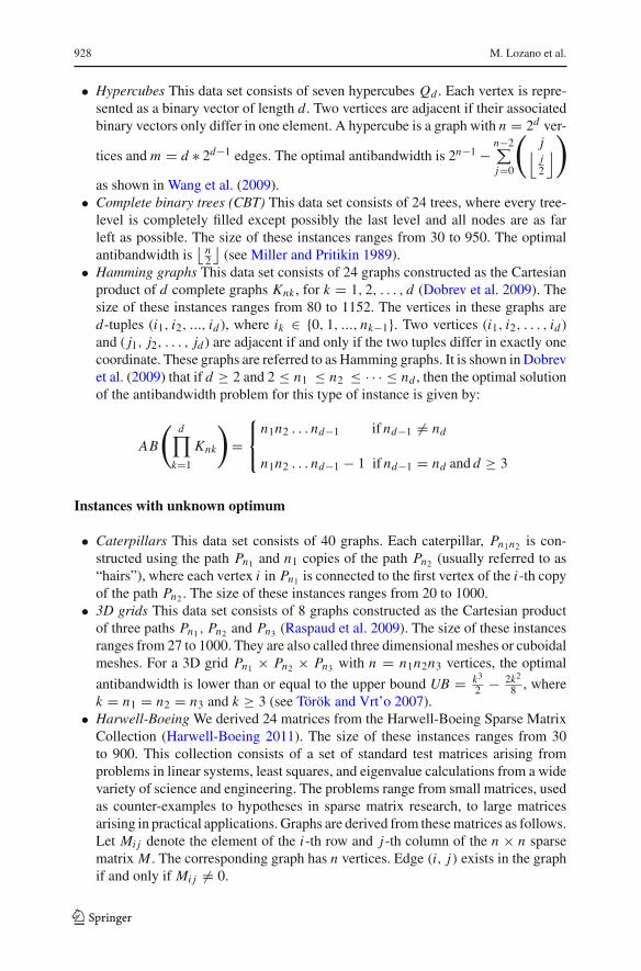
• Hypercubes This data set consists of seven hypercubes Qd . Each vertex is repre-sented as a binary vector of length d. Two vertices are adjacent if their associatedbinary vectors only differ in one element. A hypercube is a graph with n = 2d ver-

tices and m = d ∗ 2d−1 edges. The optimal antibandwidth is 2n−1 −n−2∑

j=0

(j⌊j2

⌋)

as shown in Wang et al. (2009).• Complete binary trees (CBT) This data set consists of 24 trees, where every tree-

level is completely filled except possibly the last level and all nodes are as farleft as possible. The size of these instances ranges from 30 to 950. The optimalantibandwidth is

⌊ n2

⌋(see Miller and Pritikin 1989).

• Hamming graphs This data set consists of 24 graphs constructed as the Cartesianproduct of d complete graphs Knk , for k = 1, 2, . . . , d (Dobrev et al. 2009). Thesize of these instances ranges from 80 to 1152. The vertices in these graphs ared-tuples (i1, i2, ..., id ), where ik ∈ {0, 1, ..., nk−1}. Two vertices (i1, i2, . . . , id )and ( j1, j2, . . . , jd ) are adjacent if and only if the two tuples differ in exactly onecoordinate. These graphs are referred to as Hamming graphs. It is shown in Dobrevet al. (2009) that if d ≥ 2 and 2 ≤ n1 ≤ n2 ≤ · · · ≤ nd , then the optimal solutionof the antibandwidth problem for this type of instance is given by:

AB

(d∏

k=1

Knk

)

=⎧⎨

⎩

n1n2 . . . nd−1 if nd−1 �= nd

n1n2 . . . nd−1 − 1 if nd−1 = nd and d ≥ 3

Instances with unknown optimum

• Caterpillars This data set consists of 40 graphs. Each caterpillar, Pn1n2 is con-structed using the path Pn1 and n1 copies of the path Pn2 (usually referred to as“hairs”), where each vertex i in Pn1 is connected to the first vertex of the i-th copyof the path Pn2 . The size of these instances ranges from 20 to 1000.

• 3D grids This data set consists of 8 graphs constructed as the Cartesian productof three paths Pn1, Pn2 and Pn3 (Raspaud et al. 2009). The size of these instancesranges from 27 to 1000. They are also called three dimensional meshes or cuboidalmeshes. For a 3D grid Pn1 × Pn2 × Pn3 with n = n1n2n3 vertices, the optimal

antibandwidth is lower than or equal to the upper bound UB = k3

2 − 2k2

8 , wherek = n1 = n2 = n3 and k ≥ 3 (see Török and Vrt’o 2007).

• Harwell-Boeing We derived 24 matrices from the Harwell-Boeing Sparse MatrixCollection (Harwell-Boeing 2011). The size of these instances ranges from 30to 900. This collection consists of a set of standard test matrices arising fromproblems in linear systems, least squares, and eigenvalue calculations from a widevariety of science and engineering. The problems range from small matrices, usedas counter-examples to hypotheses in sparse matrix research, to large matricesarising in practical applications. Graphs are derived from these matrices as follows.Let Mi j denote the element of the i-th row and j-th column of the n × n sparsematrix M . The corresponding graph has n vertices. Edge (i, j) exists in the graphif and only if Mi j �= 0.

123


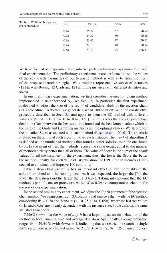
Table 1 Width of the ejectionchain procedure

|W | Dev. (%) Score Time

0.1n 25.27 67 78.72

0.2n 24.37 50 120.26

0.3n 23.42 37 159.92

0.4n 22.10 18 198.34

0.5n 21.73 25 236.43

We have divided our experimentation into two parts: preliminary experimentation andfinal experimentation. The preliminary experiments were performed to set the valuesof the key search parameters of our heuristic method as well as to show the meritof the proposed search strategies. We consider a representative subset of instances(12 Harwell-Boeing, 12 Grids and 12 Hamming instances with different densities andsizes).

In our preliminary experimentation, we first consider the ejection chain methodimplemented in neighborhood N3 (see Sect. 2). In particular, the first experimentis devoted to adjust the size of the set W of candidate labels of the ejection chain(EC) procedure. To do that, we generate a set of 100 solutions with the constructiveprocedure described in Sect. 3.1 and apply to them the EC method with differentvalues of |W | ∈ {0.1n, 0.2n, 0.3n, 0.4n, 0.5n}. Table 1 shows the average percentagedeviation (Dev.) between the best solutions found and the best known value (which inthe case of the Grids and Hamming instances are the optimal values). We also reportthe so-called Score associated with each method (Resende et al. 2010). This statisticis based on the nrank of each algorithm over each instance. The nrank of algorithm Ais defined as the number of methods that found a better solution than the one foundby A. In the event of ties, the methods receive the same nrank, equal to the numberof methods strictly better than all of them. The value of Score is the sum of the nrankvalues for all the instances in the experiment, thus, the lower the Score the betterthe method. Finally, for each value of |W | we show the CPU time in seconds (Time)needed to construct and improve 100 solutions.

Table 1 shows that size of W has an important effect in both the quality of thesolution obtained and the running time. As it was expected, the larger the |W |, thelower the deviation (and the larger the CPU time). Taking into account that the ECmethod is part of a master procedure, we set W = 0.3n as a compromise selection forthe rest of our experimentation.

In the second preliminary experiment, we adjust the depth parameter of the ejectionchain method. We again construct 100 solutions and improve them with the EC methodconsidering W = 0.3n and depth ∈ {1, 10, 25, 0.1n, 0.05n}, where the last two values(0.1n and 0.05n) are linearly dependent with the instance size. Table 2 shows the samestatistics than above.

Table 2 shows that the value of depth has a large impact on the behaviour of themethod in both, running time and average deviation. Specifically, average deviationranges from 29.44 % (with depth = 1, indicating that we restrict the search to singlemoves and there is no chained move), to 21.75 % (with depth = 25 chained moves).

123


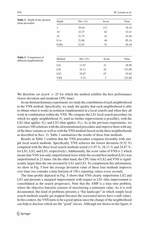
Table 2 Depth of the ejectionchain procedure

Depth Dev. (%) Score Time

1 29.44 112 18.16

10 22.37 62 32.41

25 21.75 43 42.56

0.1n 21.88 46 85.14

0.05n 22.42 51 56.44

Table 3 Comparison ofdifferent neighborhoods

Method Dev. (%) Score Time

LS1 11.97 21 58.98

LS2 16.11 44 123.00

LS3 24.87 67 55.62

VNS 9.32 2 122.88

We therefore set depth = 25 for which the method exhibits the best performance(lower deviation and moderate CPU time).

In our third preliminary experiment, we study the contribution of each neighborhoodto the VNS method. Specifically, we study the quality that each neighborhood is ableto obtain when it works in isolation (implemented in a local search) and when they allwork in combination within the VNS. We compare the LS1 local search procedure (inwhich we apply neighborhood N1 until no further improvement is possible), with theLS2 (that applies N2) and LS3 (that applies N3). As in the previous experiments, weconstruct 100 solutions with the aforementioned procedure and improve them with anyof the three variants as well as with the VNS method (based on the three neighborhoodsas described in Sect. 3). Table 3 summarizes the results of these four methods.

Results in Table 3 confirm that the VNS procedure compares favorably with sim-ple local search methods. Specifically, VNS achieves the lowest deviation (9.32 %)compared with the three local search methods tested (11.97 %, 16.11 % and 24.87 %,for LS1, LS2, and LS3, respectively). Additionally, the score value of VNS is 2 whichmeans that VNS was only outperformed twice while the second best method (LS1) wasoutperformed in 21 times. On the other hand, the CPU time of LS2 and VNS is signif-icantly larger than the one invested by LS1 and LS3. To complement this information,we show in Fig. 5 how the average deviation value of these four methods improvesover time (we consider a time horizon of 150 s reporting values every second).

The time-profile depicted in Fig. 5 shows that VNS clearly outperforms LS2 andLS3 and presents a marginal improvement with respect to LS1 (this improvement isconsolidated as the search progresses). Note that the AMP is a max–min problem,where the objective function consists of maximizing a minimum value. As it is welldocumented, this kind of problems presents a “flat landscape” in which simple localsearch methods usually get trapped (because the associated moves have a null value).In this context, the VNS turns to be a good option since the change of the neighborhoodcan help to disclose which are the “good” moves. Although not shown in this figure, it

123


10%

15%

20%

25%

30%

35%

40%

45%

50%

0 20 40 60 80 100 120 140

Dev

.

Seconds

LS1

LS2

LS3

VNS

Fig. 5 Average deviation of the best solution found over the time

is worth mentioning that even if we run LS1 for longer running times (up to 1800 s),it is not able to reach the objective function values found by VNS in the first 100 s in8 out of 36 instances.

Considering that the differences between LS1 and VNS are relatively small, wehave applied two statistical tests for pairwise comparisons, the Wilcoxon test and theSign test. The former test computes if the two samples (the solutions of both methods)come from different populations, while the latter computes the number of instanceson which an algorithm improves upon the other. The resulting p values of 0.000 and0.001 respectively, indicate that there are significant differences between the resultsof both methods, resulting VNS as the best method of this experiment.

In the final experimentation, we compare our VNS method with the best previousmethods. As described in Sect. 1, they are the Memetic Algorithm, MA, proposedby Bansal and Srivastava (2011) and the Evolutionary Path Relinking, EvPR, dueto Duarte et al. (2011). Table 4 presents the performance of each algorithm over thegroup of 164 instances with known optimum. Each main row reports the results on eachgroup of instances. In particular, we compute the average deviation (Dev.), numberof optimum (#Opt) and score of the best solutions found with each method on eachgroup of instances. The three methods are run for a similar running time (150 s) onthe same computer. Small differences on running times are due to the stopping criteria(based on the number of iterations of each method). It is important to note that the threemethods considered are able to find most of the optima if they run for long CPU times.However, in the context of heuristic optimization, the ability to find good solutions inshort running times is a key factor. In order to find significant differences among themethods and test this ability, we limit the CPU time to 150 s.

Results in Table 4 show that the VNS obtains the best solutions in four sets ofinstances (in terms of number of optima and average deviation). In particular, it isable to match the optima in the 24 instances in the Paths set, 16 optima (out of 24)and 0.84 % average deviation in the Cycles set, 1 optimum (out of 24) and 3.92 %average deviation in the CBT set, and 1 optimum (out of 24) and 17.06 % averagedeviation in the Hamming set, which compare favorably with the results obtained with

123


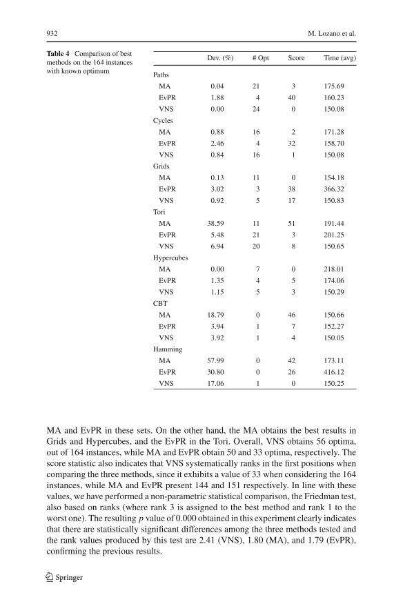
Table 4 Comparison of bestmethods on the 164 instanceswith known optimum

Dev. (%) # Opt Score Time (avg)

Paths

MA 0.04 21 3 175.69

EvPR 1.88 4 40 160.23

VNS 0.00 24 0 150.08

Cycles

MA 0.88 16 2 171.28

EvPR 2.46 4 32 158.70

VNS 0.84 16 1 150.08

Grids

MA 0.13 11 0 154.18

EvPR 3.02 3 38 366.32

VNS 0.92 5 17 150.83

Tori

MA 38.59 11 51 191.44

EvPR 5.48 21 3 201.25

VNS 6.94 20 8 150.65

Hypercubes

MA 0.00 7 0 218.01

EvPR 1.35 4 5 174.06

VNS 1.15 5 3 150.29

CBT

MA 18.79 0 46 150.66

EvPR 3.94 1 7 152.27

VNS 3.92 1 4 150.05

Hamming

MA 57.99 0 42 173.11

EvPR 30.80 0 26 416.12

VNS 17.06 1 0 150.25

MA and EvPR in these sets. On the other hand, the MA obtains the best results inGrids and Hypercubes, and the EvPR in the Tori. Overall, VNS obtains 56 optima,out of 164 instances, while MA and EvPR obtain 50 and 33 optima, respectively. Thescore statistic also indicates that VNS systematically ranks in the first positions whencomparing the three methods, since it exhibits a value of 33 when considering the 164instances, while MA and EvPR present 144 and 151 respectively. In line with thesevalues, we have performed a non-parametric statistical comparison, the Friedman test,also based on ranks (where rank 3 is assigned to the best method and rank 1 to theworst one). The resulting p value of 0.000 obtained in this experiment clearly indicatesthat there are statistically significant differences among the three methods tested andthe rank values produced by this test are 2.41 (VNS), 1.80 (MA), and 1.79 (EvPR),confirming the previous results.

123


Table 5 Comparison of bestmethods on the 72 instanceswith unknown optimum

Dev. (%) # Best Score Time (avg)

3D grids

MA 0.00 8 0 223.08

EvPR 1.17 2 7 154.30

VNS 0.92 3 5 150.50

Caterpillars

MA 3.68 0 80 201.99

EvPR 0.02 38 2 155.12

VNS 0.05 38 2 150.10

HarwellBoeing

MA 48.10 3 42 152.02

EvPR 0.94 16 9 156.30

VNS 0.21 20 4 150.04

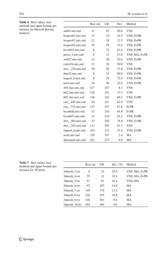
We conduct the same study over the group of instances with unknown optima(72 instances) and present the associated results in Table 5. In this case, the aver-age deviation, Dev., is computed with respect to the best known solution and #Bestindicates the number of times that each method matches the best known solution.We include in the Appendix Tables 6, 7, and 8 where we report, for each instancewith unknown optimum, the best known value, the tightest upper bound (Yixunand Jinjiang 2003), the relative deviation (in percentage) between the best knownvalue and the upper bound, and the heuristic method (or methods) achieving theseresults.

Table 5 shows that MA obtains the best results in the 3D grids set, and the worst onesin the Caterpillars and HarwellBoeing sets. On the other hand, VNS obtains the bestresults in the HarwellBoeing set and ranks second in the other two sets. Overall resultson the 72 instances show that VNS presents an average percentage deviation of 0.39 %and 61 best-known values, followed by EvPR (with 0.71 % and 56 respectively), andMA (with 25.89 % and 11). The resulting p value of 0.000 obtained with the Friedmantest in this experiment certifies that there are differences among these three methods,and the associated rank values of 2.42 (VNS), 2.33 (EvPR) and 1.26 (MA) are in linewith the pattern shown above.

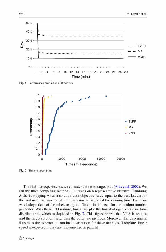
In order to evaluate the behavior of these methods over a long-term time horizon,we run MA, EvPR and VNS for 30 min, reporting the average deviation of the bestfound solution every minute. We consider the set of 36 representative instances usedin the preliminary experimentation. Figure 6 shows the corresponding average timeprofile, in which we can see that VNS consistently produces better results than itscompetitors although the three of them are able to produce good results. Specifically,the three methods quickly improve its average deviation in the first two minutes inwhich VNS clearly establishes its superiority. From this point, the methods are onlyable to produce a marginal improvement (around 1 %), which on the other hand is adifficult task considering the max–min of this optimization problem.

123


0%

10%

20%

30%

40%

50%

0 2 4 6 8 10 12 14 16 18 20 22 24 26 28 30

Dev

.

Time (min.)

EvPR

MA

VNS

Fig. 6 Performance profile for a 30 min run

0

0.1

0.2

0.3

0.4

0.5

0.6

0.7

0.8

0.9

1

0 5000 10000 15000 20000

Pro

bab

ility

Time (milliseconds)

EvPR

MA

VNS

Fig. 7 Time to target plots

To finish our experiments, we consider a time-to-target plot (Aiex et al. 2002). Weran the three competing methods 100 times on a representative instance, Hamming5×6×6, stopping when a solution with objective value equal to the best known forthis instance, 16, was found. For each run we recorded the running time. Each runwas independent of the other, using a different initial seed for the random numbergenerator. With these 100 running times, we plot the time-to-target plots (run timedistributions), which is depicted in Fig. 7. This figure shows that VNS is able tofind the target solution faster than the other two methods. Moreover, this experimentillustrates the exponential runtime distribution for these methods. Therefore, linearspeed is expected if they are implemented in parallel.

123


5 Conclusions

In this paper, we report our research on the use of different neighbours and candidate liststrategies that allows us to cope with a computationally expensive objective functionevaluation within a VNS procedure with ejection chains. Our procedure selects movesfrom a candidate list of moves whose move values are not updated after every iteration.The list follows the tabu search principle that the values of a set of elite moves do notdrastically change from one iteration to the next and therefore it is not necessary toupdate them after the execution of every move. In addition to the application of thiscandidate list strategy, our procedure employs an unconventional definition of movevalue, which is not based on the change of the objective function value to direct thesearch. In this way, our move value definition conveys information that is not availablewhen the change in the objective function value is calculated.

The performance of the procedure has been assessed using 236 problem instancesof several types and sizes. Our preliminary experimentation clearly proves the merit ofcombine neighborhoods, as VNS does, in the context of max–min problems. Moreover,the procedure has been shown robust in terms of solution quality within a reasonablecomputational effort. The proposed method was compared with two recently developedprocedures due to Duarte et al. (2011) and Bansal and Srivastava (2011) respectively.The comparisons favor the proposed variable neighborhood search implementation.

According to our experimentation, the Paths, Cycles, Grids and Hypercubeinstances can be considered “easy to solve”. On the contrary, the CBT, Hammingand HarwellBoeing instances are actually a challenge for modern heuristic methods.

Acknowledgements This research has been partially supported by the Ministerio de Ciencia e Inno-vación of Spain within the OPTSICOM project (http://www.optsicom.es/) with grant codes TIN2008-05854,TIN2009-07516, TIN2012-35632, and P08-TIC-4173.

Appendix

Tables 6, 7 and 8 report the comparison of the state-of-the-art methods over the setof instances with unknown optimum. We consider a time limit of 150 s per instance.Each table shows for each instance the best known value, Best val., the tightest upperbound (Yixun and Jinjiang 2003), UB, the relative deviation (in percentage) betweenthe best known value and the upper bound, Dev, and finally the heuristic method (ormethods) achieving these results.

123

http://www.optsicom.es/


Table 6 Best values, bestmethods and upper bounds perinstance for Harwell-Boeingmatrices

Best val. UB Dev Method

ash85.mtx.rnd 21 42 50.0 VNS

bcspwr01.mtx.rnd 17 19 10.5 VNS, EvPR



bcsstk01.mtx.rnd 8 22 63.6 VNS, EvPR

pores_1.mtx.rnd 6 13 53.8 VNS, MA, EvPR

will57.mtx.rnd 13 28 53.6 VNS, EvPR

curtis54.mtx.rnd 13 26 50.0 VNS

dwt__234.mtx.rnd 50 58 13.8 VNS, EvPR

ibm32.mtx.rnd 9 15 40.0 VNS, EvPR

impcol_b.mtx.rnd 8 29 72.4 VNS, EvPR

nos4.mtx.rnd 34 50 32.0 VNS, EvPR

494_bus.mtx.rnd 227 247 8.1 VNS

662_bus.mtx.rnd 220 331 33.5 VNS

685_bus.mtx.rnd 136 342 60.2 VNS, EvPR

can__445.mtx.rnd 82 221 62.9 VNS

can__715.mtx.rnd 115 357 67.8 EvPR

bcsstk06.mtx.rnd 32 210 84.8 EvPR

bcsstk07.mtx.rnd 31 210 85.2 VNS, EvPR

dwt__503.mtx.rnd 53 250 78.8 VNS, EvPR

dwt__592.mtx.rnd 113 295 61.7 VNS

impcol_d.mtx.rnd 103 212 51.4 VNS, EvPR

nos6.mtx.rnd 329 337 2.4 MA

sherman4.mtx.rnd 261 272 4.0 MA

Table 7 Best values, bestmethods and upper bounds perinstance for 3D grids

Best val. UB Dev. (%) Method

3dmesh_3.txt 9 12 25.0 VNS, MA, EvPR

3dmesh_4.txt 25 31 19.4 VNS, MA, EvPR

3dmesh_5.txt 51 61 16.4 VNS, MA

3dmesh_6.txt 92 107 14.0 MA

3dmesh_7.txt 149 170 12.4 MA

3dmesh_8.txt 228 255 10.6 MA

3dmesh_9.txt 328 363 9.6 MA

3dmesh_10.txt 454 499 9.0 MA

123


Table 8 Best values, bestmethods and upper bounds perinstance for Caterpillars

Best val. UB Dev. (%) Method

caterpillar_5_4.txt 10 10 0.0 VNS, EvPR


















caterpillar_20_6.txt 60 60 0.0 EvPR



caterpillar_20_15.txt 148 150 1.3% VNS, EvPR


caterpillar_20_25.txt 247 250 1.2 EvPR




caterpillar_25_25.txt 309 312 1.0 VNS






caterpillar_35_15.txt 260 262 0.8 VNS







123


References

Aiex, R.M., Resende, M.G.C., Ribeiro, C.C.: Probability distribution of solution time in GRASP: Anexperimental investigation. J. Heuristics 8, 343–373 (2002)

Bansal, R., Srivastava, K.: Memetic algorithm for the antibandwidth maximization problem. J. Heuristics17, 39–60 (2011)

Burkard, R.E., Donnani, H., Lin, Y., Rote, G.: The obnoxious center problem on a tree. SIAM J. Discret.Math. 14(4), 498–590 (2001)

Cappanera, P.: A survey on obnoxious facility location problems. Technical Report TR-99-11, Dipartimentodi Informatica, Università di Pisa (1999)

Díaz, J., Petit, J., Serna, M.: A survey of graph layout problems. J. ACM Comput. Surv. 34(3), 313–356(2002)

Dobrev, S., Královic, R., Pardubská, D., Török, L., Vrt’o, I.: Antibandwidth and cyclic antibandwidth ofHamming graphs. Electron. Notes Discret. Math. 34, 295–300 (2009)

Duarte, A., Martí, R., Resende, M.G.C., Silva, R.M.A.: GRASP with path relinking heuristics for theantibandwidth problem. Networks 58(3), 171–189 (2011)

Duarte, A., Escudero, L.F., Martí, R., Mladenovic, N., Pantrigo, J.J., Sánchez-Oro, J.: Variable neighborhoodsearch for the vertex separation problem. Comput. Oper. Res. 39(12), 3247–3255 (2012)

Glover, F., Laguna, M.: Tabu Search. Kluwer, Norwell (1997)Hale, W.K.: Frequency assignment: theory and applications. Proc. IEEE 68, 1497–1514 (1980)Hansen, P., Mladenovic, N., Brimberg, J., Moreno-Pérez, J.A.: Variable neighborhood search. In: Gendreau,

M., Potvin, J.-Y. (eds.) Handbook of Metaheuristics, 2nd edn, pp. 61–86. Springer, Heidelberg (2010)Harwell-Boeing: http://math.nist.gov/MatrixMarket/data/Harwell-Boeing/ (2011)Leung, J.Y.-T., Vornberger, O., Witthoff, J.D.: On some variants of the bandwidth minimization problem.

SIAM J. Comput. 13, 650–667 (1984)Martí, R., Duarte, A., Laguna, M.: Advanced scatter search for the max-cut problem. INFORMS J. Comput.

21(1), 26–38 (2009)Miller, Z., Pritikin, D.: On the separation number of a graph. Networks 19, 651–666 (1989)Pantrigo, J.J., Martí, R., Duarte, A., Pardo, E.G.: Scatter search for the cutwidth minimization problem.

Ann. Oper. Res. 199(1), 285–304 (2012)Piñana, E., Plana, I., Campos, V., Martí, R.: GRASP and path relinking for the matrix bandwidth minimiza-

tion. Eur. J. Oper. Res. 153, 200–210 (2004)Raspaud, A., Schröder, H., Sykora, O., Török, L., Vrt’o, I.: Antibandwidth and cyclic antibandwidth of

meshes and hypercubes. Discret. Math. 309, 3541–3552 (2009)Rego, C.: Node ejection chains for the vehicle routing problem: sequential and parallel algorithms. Parallel

Comput. 27(3), 201–222 (2001)Resende, M., Martí, R., Gallego, M., Duarte, A.: GRASP and path relinking for the max-min diversity

problem. Comput. Oper. Res. 37, 498–508 (2010)Rodriguez-Tello, E., Jin-Kao, H., Torres-Jimenez, J.: An effective two-stage simulated annealing algorithm

for the minimum linear arrangement problem. Comput. Oper. Res. 35(10), 3331–3346 (2008)Török, L., Vrt’o, I.: Antibandwidth of 3-dimensional meshes. Electron. Notes Discret. Math. 28, 161–167

(2007)Yixun, L., Jinjiang, Y.: The dual bandwidth problem for graphs. J. Zhengzhou Univ. 35, 1–5 (2003)Wang, X., Wu, X., Dumitrescu, S.: On explicit formulas for bandwidth and antibandwidth of hypercubes.

Discret. Appl. Math. 157(8), 1947–1952 (2009)

123

http://math.nist.gov/MatrixMarket/data/Harwell-Boeing/

variable neighborhood search with ejection chains for...

Documents