valuation of tax loss carryforwards

ORI GINAL RESEARCH

Valuation of tax loss carryforwards

Sudipto Sarkar

� Springer Science+Business Media New York 2013

Abstract Tax loss carryforwards (TLC) are a valuable asset because they can potentially

reduce a company’s future tax payments. However, there is often a great deal of uncer-

tainty regarding the probability and timing of these tax savings. We propose a contingent-

claim model to value this asset. The value is determined primarily by the size of accu-

mulated carryforwards relative to earnings. We show that, for poorly performing firms with

large TLC, (1) the realizable (or fair) value of the tax losses can be significantly smaller

than the book value, and (2) the tax losses can account for a significant fraction of the

company’s equity value. The model is illustrated by calibrating it to a couple of companies

with large carryforwards. Finally, we show how the model can be used to compute the

marginal tax rate of a company with carryforwards.

Keywords Tax loss carryforwards � Net operating losses � Valuation �Contingent-claim model

JEL Classification G3.

1 Introduction

The objective of this paper is to value explicitly a common intangible corporate asset—tax

loss carryforwards (TLC) or net operating losses (NOL).1 This asset is valuable because of

S. Sarkar (&)DSB 302, McMaster University, Hamilton, ON L8S 4M4, Canadae-mail: [email protected]

1 A large number of firms have accumulated tax losses (Graham 1996a; Miller and Skinner 1998; Baumanand Das 2004); a look at the 2008–2009 annual statements in Compustat reveals that, after deleting firmswith missing data, about 75 % of US firms (3,989 out of 5,291) were carrying tax losses. Moreover, taxlosses can be significant in terms of magnitude; for instance, tax carryforwards accounted for 30.4 % of totalassets in the Bauman and Das (2004) sample of internet firms, while firms in the Miller and Skinner (1998)sample had average deferred tax assets of about 10 % of total assets.

123

Rev Quant Finan AccDOI 10.1007/s11156-013-0393-5

its ability to shelter a part of the firm’s future income from taxation. The book value of

such an asset is simply the tax rate times the amount of the TLC. However, the actual

(realizable) value is uncertain because of the volatile nature of future income, uncertainty

about the timing of the tax benefits, and the risk of bankruptcy.

We use a contingent-claim valuation model, which has been used in the Finance lit-

erature to value a firm’s securities (Leland 1994), earnings (Goldstein et al. 2001), growth

opportunities (Tserlukevich 2008), information technology investments (Lee et al. 2009),

and intangible assets such as patents (Pakes 1986; Schwartz 2004) and debt tax shields

(Couch et al. 2012).

De Waegenaere et al. (2003) explicitly value TLC, but there is no earnings uncertainty

or bankruptcy risk in their model; once realized, the firm’s income is a constant stream, and

if it is negative the firm abandons the project while if it is positive the (pre-existing) TLC is

reduced at a constant rate until it is all used up or the expiry date is reached, whichever

comes first. Given that earnings uncertainty is an important factor in valuing TLC, it would

seem reasonable to incorporate uncertainty in the valuation model.

We extend De Waegenaere et al. (2003) by incorporating earnings volatility and

bankruptcy risk in the model. Thus, the earnings stream in our model is a random

process, and the taxable income can be positive or negative, depending on the operating

earnings realization and the debt level. As a result, TLC can rise or fall over time,

depending on the profit or loss. Further, our model includes bankruptcy risk, i.e., if the

earnings fall sufficiently, the company can declare bankruptcy. Bankruptcy risk will be

an important consideration for firms with significant accumulated TLC (which indicates

poor financial condition, such as extended loss-making periods and/or leverage ratios

that are too high), hence bankruptcy risk should be taken into account when valuing

TLC. To summarize, in our model: (1) the earnings process is random, (2) taxable

income can be positive or negative, (3) TLC can rise or fall, and (4) there is bank-

ruptcy risk.

We compute the fair (realizable, or market) value of the firm’s TLC in a parsimonious

way, with a small number of inputs—the properties of the firm’s earnings (level, growth

rate and volatility), the debt level, amount of TLC, interest rate and tax rate. The market (or

fair) value of TLC is smaller than the book value, as expected, and can be substantially

smaller for companies which have large TLC relative to earnings, particularly when

earnings growth is low. For such firms, TLC can make a significant contribution to equity

value. We show how the model can be used by calibrating it to two companies with large

TLC in 2009—Boeing Corp. and Office Max. Finally, we show how the model can be used

to extract the marginal tax rate (MTR) of a company with TLC, which can be considerably

smaller than the statutory tax rate if TLC is large relative to earnings.

Apart from its use for valuation purposes and computing the MTR, such a model has

other possible applications, e.g., examining the effect of TLC on capital structure, or in

corporate reporting of TLC (the Deferred Tax Asset Valuation Allowance under SFAS

109, see Jeter et al. 2008). As pointed out in the Accounting literature, it is tempting for

managers to use the Deferred Tax Asset Valuation Allowance Account (VAA) for

earnings management purposes (Frank and Rego 2006). If TLC can be valued with

some confidence, it will be difficult to exploit its reporting for earnings management

purposes.

The rest of the paper is organized as follows. Section 2 describes the valuation model,

Sect. 3 derives and discusses the results, Sect. 4 suggests an application of the model to

MTRs, and Sect. 5 summarizes and concludes.

S. Sarkar

123

2 The valuation model for TLC

A tax loss carryforward is valuable because it can be used to reduce taxable income and

therefore reduce the firm’s tax payments in future. Suppose the firm’s profits are taxed at a

rate of s, and it has accumulated TLC of $L. Then the firm can use this to reduce its taxable

income by $L, hence it can reduce its tax bill (and therefore increase firm value) by $sL.

This is the book value of the TLC, and represents the value of the TLC if the firm could

utilize all of it immediately. Thus, the book value is the upper limit of the actual (market,

or realizable) value of the TLC. The market value would be lower than the book value

because of the following:

1. The TLC cannot necessarily be fully utilized immediately. The company must first

make sufficient profits, and this might happen only after a period of time. Because of

the delay (time value and discounting), the actual value of the TLC will be smaller

than the book value (see, for instance, Lei et al. 2013). Moreover, if the company

continues to make losses, the TLC will rise by the amount of the losses, hence there

will a further delay in realizing the benefits, and this will further reduce the realizable

value.

2. If the company’s performance deteriorates further, and it files for bankruptcy (which is

quite possible in loss-making firms), then the accumulated TLC will be substantially

lost. Thus, the value of the TLC will shrink as bankruptcy risk increases.

3. The TLC can be carried forward only for a limited number of years (20 years in the

US).

Thus, the actual value will be smaller than the book value $sL; how much smaller

depends on a number of factors. For instance, if TLC is large relative to earnings, it is less

likely that the TLC can be fully utilized in a timely manner, hence it is less valuable. The

valuation is complicated by the uncertain nature of the earnings stream (see Baez-Diaz

and Alam 2013). The fundamental determinant of TLC value is the random earnings level

(current and future) of the firm, relative to the accumulated TLC. If earnings decline, the

timely realization of the tax benefits becomes less likely and the value of the TLC will

fall. Similarly, a rise in earnings will make the timely utilization of TLC more likely, and

thus increase its value. The value of the TLC is therefore contingent on the uncertain

stream of future earnings. It can then be valued as a contingent claim on the firm’s

random earnings. This is what we propose—a contingent-claim model to value TLC as a

function of the firm’s earnings level, taking into account the random nature of the

earnings process and the fact that TLC can change randomly in either direction depending

on earnings.

2.1 Model basics

We extend the basic contingent-claim model (Leland 1994; Goldstein et al. 2001) to

include a second state variable, the magnitude of the accumulated TLC. The firm’s

operating earnings (cash from operations, or EBITDA) is given by a random stream of $xt

per unit time, which follows a lognormal (or Geometric Brownian Motion) process:

dx=x ¼ l dt þ r dz ð1Þ

where l and r are the drift and volatility parameters (both constant), respectively, and z is

a standard Wiener process. This is a standard way of modeling corporate operating cash


123

flows, e.g., Goldstein et al. (2001), Broadie et al. (2007), Hackbarth and Mauer (2012),

Hackbarth et al. (2007), Parrino et al. (2005), Purnanandam (2008).2,3

The company has outstanding long-term (perpetual) debt with a coupon payment of $c

per unit time.4 This coupon will continue in perpetuity unless the firm files for bankruptcy,

in which case the bondholders will become the company’s owners and take over the assets

of the firm. Thus the company’s taxable earnings are given by (x–c) per unit time, which

can be negative if the operating earnings x are smaller than the coupon obligation c.5 The

taxable earnings, (x–c), when positive, are taxed at the corporate tax rate of s. However,

the tax rate is zero for losses, i.e., there are no tax rebates for losses.

Thus the company’s tax rate is zero for losses and s ([0) for profits. Because of this

asymmetry in the tax rates, the tax schedule in our model is convex or progressive,

consistent with most tax schedules in the real world (Graham and Smith 1999). As stated

by Graham and Smith (1999, p. 2243, Section I.A), ‘‘…, the major source of tax function

convexity is the asymmetric treatment of gains and losses—a tax rate of zero for losses but

positive tax rates on profits.’’6

However, while no rebates are given for incurring losses, the losses can be accumulated

for tax purposes and carried forward as accumulated NOL or TLC; when the firm turns

profitable again, the taxable profit is reduced by the accumulated losses. We assume that

the firm currently has accumulated tax losses of $L.

In practice, there is a limit to how long tax losses can be carried forward. However, this

limit is generally quite long, e.g., 20 years in the U.S. Therefore, for tractability, we

assume that the tax losses can be carried forward indefinitely (or until bankruptcy). This

2 There are some papers on this topic that use a random walk process to model the earnings stream, e.g.,Graham (1996a, b), Shevlin (1990). However, this way of modeling earnings has a significant drawback, i.e.,earnings volatility will be significantly under-estimated under the random walk process. This has beenpointed out and discussed at some length in a recent paper by Blouin et al. (2010). Given this weakness ofthe random walk process, it is not surprising that the contingent-claim modeling literature has extensivelyused the lognormal process for this purpose, including the papers just mentioned above. If we had used therandom walk process instead of lognormal, the earnings volatility would have been under-estimated in ourmodel; as a result, both the TLC value and the marginal tax rate (MTR) would have been over-estimated byour model.3 The lognormal process, while a popular way of modeling earning in the Finance literature, is not the onlyprocess that can be used to depict the earnings process. In the early Accounting literature, for instance, somepapers showed empirical support for the random walk, seasonal random walk with drift and other ARprocesses (Lev 1983; Lang 1991), although other papers disagreed with this (Lieber et al. 1983; Freemanet al. 1982). Further, Lipe and Kormendi (1994) provided evidence of mean reversion in the earningsprocess. In the trade-off between tractability and realism, we use the lognormal process that is commonlyused in the Finance literature.4 Constant coupon payment is a simplifying assumption for reasons of tractability. In real life, companiestend to reduce debt level when the benefits of debt are smaller (as in the case of large TLC). Reducing debtlevel will result in higher TLC values, since (as shown later in the paper) a lower leverage ratio increasesTLC value, everything else remaining unchanged. On the other hand, companies with large TLC aregenerally in financial trouble and might not have the necessary cash to buy back debt. Hence the final effectof this is not clear and must be evaluated on a case-by-case basis.5 Even if earnings are negative, the company does not necessarily default on its debt. This assumption mightraise the question: where does the money to make coupon payment come from? We make the implicitassumption, as in Leland (1994), Goldstein et al. (2001), etc., that this money comes from shareholders. Theargument is as follows. As long as the equity has some value, rational shareholders will keep the companyalive even if they have to make out-of-pocket payments (see Leland 1994 for the detailed argument). Thisargument also has empirical support (Bhagat et al. 2005).6 There is also some statutory progressivity, as pointed out by Graham and Smith (1999, p. 2243), becausethere are two tax rates: 15 % if profits are below $100,000 and 34 % if profits exceed $100,000. We examinethe effect of this statutory progressivity in Sect. 3.2.

S. Sarkar

123

means our model will somewhat overstate the value of a TLC; however, the difference

should be small, since the time limit is generally quite long, as mentioned above.

As in Goldstein et al. (2001) and the other papers cited above, when x falls to a

sufficiently low level (say x = xd), the firm will file for bankruptcy, at which time the

model ends. When the company files for bankruptcy, the payoff to equity holders is zero,

and bondholders acquire control of the assets of the company. Finally, the constant risk-

free interest rate is given by r.

In the next two sections, we value the equity of a company with accumulated tax losses.

As a benchmark, we also compute (in Appendix 2) the value of the firm’s equity when TLC

are not allowed.

2.2 Cash flow to shareholders and evolution of TLC

With operating earnings of x and coupon payment of c, the pre-tax profit stream to

shareholders is $(x–c) per unit time, and can be positive or negative.7 However, the

accumulated TLC cannot be negative, i.e., L C 0. Thus, four different scenarios are

possible (similar to Shevlin 1990):

1. Profit-making firm with TLC (L [ 0 and x C c)

2. Loss-making firm with TLC (L [ 0 and x \ c)

3. Profit-making firm with no TLC (L = 0 and x C c), and

4. Loss-making firm with no TLC (L = 0 and x \ c).

We discuss below the after-tax cash flow to equity holders and the evolution of the

accumulated TLC for each scenario.8

1. L [ 0 and x C c: Here the firm is profitable and would normally pay tax of $s (x–c)

per unit time. However, the firm has accumulated TLC, which it will use to offset the

income for tax purposes; thus, as long as L [ 0, the firm pays no taxes,9 and the after-

tax cash flow stream is $(x–c) per unit time. The TLC is utilized at a rate of –(x–c)

dt = (c–x)dt. Thus, the TLC will be shrinking at the same rate that it is used up to

offset taxable income, hence dL = (c–x)dt. Therefore, for this scenario, we have: net

after-tax cash flow to shareholders = $(x–c) per unit time, and dL = (c–x) dt.

2. L [ 0 and x \ c: Since the firm is making losses, it will not pay any taxes anyway;

thus, the after-tax cash flow to shareholders = $(x–c) per unit time (note that this is

negative, so shareholders will finance this, as discussed in footnote 5). Also, since the

7 We assume, as in Leland (1994), that cash shortfalls are met by shareholders. Thus, when cash fromoperations fall short of the company’s coupon obligation (x \ c), shareholders keep the company alive bypaying the difference. If, however, earnings fall to a sufficiently low level, shareholders will not find itworthwhile to keep the company alive, and the company will file for bankruptcy (as in Leland 1994;Goldstein et al. 2001). This is consistent with actual corporate and shareholder behavior; as Bhagat et al.(2005) show, in loss-making firms it is the equity holders who invest in the company in order to keep it alive.8 In Shevlin’s (1990) study of marginal corporate tax rates with NOL, there are four scenarios (see hisTable 1): (a) negative taxable income and zero NOL, (b) negative taxable income and positive NOL,(c) positive taxable income and zero NOL, and (d) positive taxable income and positive NOL. In our model,the corresponding scenarios are (4), (2), (3) and (1) respectively.9 This is because of the continuous-time nature of the model. In a discrete-time model, at year-end theoutstanding TLC might be smaller than the taxable profit, in which case there would be a tax liability. In acontinuous-time model, tax is paid continuously, but only after L is exhausted; therefore, when the companypays taxes, we must have L = 0. After L is exhausted, the firm is in region (3) and will be paying tax.


123

company is incurring losses, the accumulated TLC will increase at the same rate that

the firm is making losses, i.e., dL = (c–x) dt.

3. L = 0 and x C c: In this scenario, the firm is profitable and has no TLC, hence it is

taxed at the rate s, and the cash flow to equity holders is (1–s)(x–c) per unit time. Since

there are no TLC being created or used up, we have dL = 0.

4. L = 0 and x \ c: When the company is making losses, it will (by definition) have

positive TLC. Thus, when x \ c, it is not possible to have L = 0. This scenario is

therefore not feasible in the model. (This would not necessarily be true if tax

carrybacks were allowed in the model).

From the above discussion, we can see that there will effectively be two operating

regions in our model:

Region I [L [ 0, cash flow to shareholders = (x–c) per unit time, and dL = (c–x) dt];

Region II [L = 0, cash flow to equity holders = (1–s)(x–c) per unit time, and dL = 0].

2.3 Equity valuation

Equity is a contingent claim (hence a function of x), as in Goldstein et al. (2001) and the

other papers mentioned above. Because of the perpetual setting of the model, the equity

value will be time-independent. Also, equity value will be a function of L in Region I but

independent of L in Region II. Therefore, equity value will have to be evaluated separately

for each region. Note that the firm can move from Region I to Region II when TLC are

exhausted, and back to Region I when it picks up TLC again [see boundary conditions,

Eqs. (13) and (14)].

2.3.1 Region I (L [ 0)

This is the region in which the company has TLC of $L. Since these carryforwards are

valuable, equity value will be a function of L. Let the equity value in this region be V(x, L).

Then, as shown in Appendix 1, V(x, L) must satisfy the following partial differential

equation (PDE):

0:5r2x2 Vxxðx,LÞ þ lxVxðx,LÞ � rVðx,LÞ þ ðc� xÞVLðx,LÞ þ x� c ¼ 0 ð2Þ

where subscripts denote partial derivatives. This PDE has to be solved, subject to the

appropriate boundary conditions, for the equity value V(x,L).

2.3.2 Region II (L = 0)

In this region, equity value is just a function of x, say U(x). Then, as shown in Appendix 1,

U(x) must satisfy the ordinary differential equation (ODE):

0:5r2x2 U00ðxÞ þ lxU0ðxÞ � rUðxÞ þ ð1� sÞðx� cÞ ¼ 0 ð3Þ

where U0ðxÞ and U00ðxÞ are first and second derivatives. The solution to this ODE is:

U(x) ¼ ð1� sÞ x

r� l� c

r

� �þ Axc1 þ Bxc2 ð4Þ

where A and B will be determined by boundary conditions, and c1 ([0) and c2 (\0) are

solutions of the quadratic equation:

S. Sarkar

123

0:5r2cðc� 1Þ þ lc� r ¼ 0 ð5Þ

and are given by

c1 ¼ 0:5� l=r2 þffiffiffiffiffiffiffiffiffiffiffiffiffiffiffiffiffiffiffiffiffiffiffiffiffiffiffiffiffiffiffiffiffiffiffiffiffiffiffiffiffiffi0:5� l=r2ð Þ2þ2r=r2

qð6Þ

c2 ¼ 0:5� l=r2 �ffiffiffiffiffiffiffiffiffiffiffiffiffiffiffiffiffiffiffiffiffiffiffiffiffiffiffiffiffiffiffiffiffiffiffiffiffiffiffiffiffiffi0:5� l=r2ð Þ2þ2r=r2

qð7Þ

The first term of Eq. (4) is simply the expected present value, to shareholders, of

operating forever in Region II. The other two terms reflect the effects of the boundary

x = c (moving to Region I) and the boundary x ? ?. As x ? ?, the probability of

falling to Region I approaches zero, hence

U(x)! ð1� sÞ x=ðr� lÞ � c=rð Þ ð8ÞThis implies A = 0 in Eq. (4), hence we write the equity value in Region II as:

U(x) ¼ ð1� sÞ x=ðr� lÞ � c=rð Þ þ Bxc2 ð9Þ

2.3.3 Boundary conditions for V(x,L)

1. As x ? ? (earnings reach very high levels), the default risk is negligible, hence the

equity value approaches the no-default value ð1� sÞ x=ðr� lÞ � c=r½ �; also, since

earnings are so high, any accumulated TLC can be utilized completely and immedi-

ately, hence the market value of the TLC is just the book value sL. This gives the

condition:

Limx!1

V(x,L) ¼ ð1� sÞ x=ðr� lÞ � c/r½ � þ sL ð10Þ

2. At default [x = xd(L)], which occurs in Region I, the equity value must be zero, i.e.,

V xd Lð Þ;Lð Þ ¼ 0; 8L ð11ÞNote that we write the default trigger as xd(L). This is because a firm with large TLC would

presumably want to keep the firm alive longer, in order to utilize the TLC in the future,

when things turn around and the firm becomes profitable. Thus, the default trigger should

be a function of L, i.e., xd = xd(L); moreover, it is expected to be a decreasing function of

L, x0dðLÞ\0.

For the default trigger to be optimal, it must satisfy the smooth-pasting condition

(Leland 1994):

VxðxdðLÞ;LÞ ¼ 0; 8L ð12Þ

3. The firm will move between Regions I and II depending on the value of L; the

boundary between the two regions is L = 0. This gives the following boundary

conditions: at L = 0, the two functions and their derivatives must be equal, to ensure

continuity and no-arbitrage:


123

V x; 0ð Þ ¼ U xð Þ; 8x ð13Þ

Vxðx; 0Þ ¼ U0ðxÞ; 8x ð14Þ

where V(x,L) is the solution to Eq. (2) and U(x) is given by Eq. (9).

The solution to the system of Eqs. (2) and (9)–(14) will give V(x,L), the value of the

equity of the firm for a given x and a given L. Unfortunately there is no analytical solution

for this system of equations, hence V(x,L) has to be computed using numerical methods.

2.4 Value of tax loss carryforward

The equity value with TLC of L is V(x,L), calculated above. If the firm has no TLC, its

equity value will be V(x,0). The difference between the two gives the fair (market) value of

the TLC:

Market Value of TLC ¼ V x;Lð Þ � V x; 0ð Þ ð15ÞRecall that the book value of the TLC is given by sL. Therefore, the TLC’s Market-to-

Book ratio is [V(x,L) - V(x,0)]/(sL).

2.5 Implementing the numerical solution

The PDE (2) is solved numerically, by discretizing the equation in a trinomial grid. The

discretized equation is solved iteratively using the implicit finite-difference method

described by Hull (2006). Even with this approximation (resulting from discretization), the

above system of equations is quite complicated, hence we had to make a few simplifying

assumptions, as described below.

2.5.1 Boundary conditions

1. Upper limit for x (x ? ?). In order to use the boundary condition (10) in the

numerical implementation, we need to specify a maximum value of x to correspond

with the condition x ? ?. Let the limiting value of x be xMax. Then the boundary

condition (10) is approximated by

VðxMax;LÞ ¼ ð1� sÞ xMax

r� l� c

r

� �þ sL ð16Þ

That is, default risk is assumed to be zero at x = xMax instead of x ? ?. Because we use a

finite upper limit x = xMax rather than x ? ?, it means that the model will somewhat

overstate the value of the TLC. To minimize the effect of this approximation, we choose

xMax to be large enough so that default risk is virtually zero for practical purposes. In our

numerical analysis, we use c = 1 and xMax = 50, for an interest coverage ratio of 50. With

this large a coverage ratio, default risk should be negligible and any TLC can be expected

to be used up immediately, hence the effect of this simplifying assumption should be small,

and we feel that Eq. (16) is a reasonably good approximation.10

10 Bonds of companies with interest coverage ratio of over 8.5 (12.5 for smaller and riskier firms) are ratedAAA, which is the highest safety rating possible and denotes negligible bankruptcy risk (for bond ratingsand associated coverage ratios, please see http://pages.stern.nyu.edu/*adamodar/New_Home_Page/datafile/ratings.htm). Therefore, a coverage ratio of 50 should imply negligible bankruptcy risk.

S. Sarkar

123

http://pages.stern.nyu.edu/~adamodar/New_Home_Page/datafile/ratings.htm

http://pages.stern.nyu.edu/~adamodar/New_Home_Page/datafile/ratings.htm

2. Lower limit for x [default trigger, x = xd(L)]. Since the default trigger is a function of

L, it is a floating (not fixed) boundary, to be determined as part of the solution. With

the implicit finite-difference numerical method, it was not possible to solve the PDE

(2) with a floating boundary. We therefore make the simplifying assumption that the

default boundary is fixed, independent of L. Thus the default boundary is a constant, xd

(or xd(0)). This default boundary is calculated from Eq. (33) in Appendix 2, i.e., when

the firm is not allowed to carry forward any TLC.

This approximation will result in our model understating the market value of the TLC,

because one of the benefits of the carryforwards (reducing the default trigger) is being

ignored. However, this benefit is small compared to the major benefit (reduction of taxes),

hence this should also be a reasonable approximation.

3. Lower limit on L (L = 0). For the iterative solution of PDE (2), the boundary

conditions have to be explicitly specified. The natural boundary conditions that arise

from the economics of the problem (Eqs. 13, 14) are, unfortunately, implicit

conditions since the function U(x) is not known (and must be simultaneously solved

for). We therefore approximate these conditions with a simplified version, by setting

V(x,0) = E(x), 8x, where E(x) is the equity value when carryforwards are not allowed

(from Appendix 2). This is an approximation because it ignores the possibility, when

L = 0, that L might become positive some time in the future. Therefore, our numerical

procedure will understate somewhat the value of the carryforwards.

With the above simplified boundary conditions, PDE (2) is solved numerically, using a

MATLAB program. The program takes a few seconds (at most) to return the results, and is

fairly robust in that it converges to the solution rapidly in most cases.

3 Results

3.1 Base-case parameter values

Since the model is solved numerically, we have to choose a set of input parameter values to

illustrate the results. The required input parameters are the earnings level (x), earnings

growth rate (l), earnings volatility (r), debt or coupon level (c), risk-free interest rate (r),

corporate tax rate (s), and the accumulated TLC (L). We illustrate the results using a base-

case set of parameter values, and later we calibrate the model to a couple of actual

companies. The base case parameters are as follows. The earnings growth rate is set at

l = 2 %, since the cases of interest (e.g., when market value deviates significantly from

book value) involve low- or negative-growth firms. Also, firms with large TLCs tend to be

more volatile, hence we set are the earnings volatility to r = 30 %. The interest rate is

r = 6 %, and the statutory tax rate is s = 35 %. The debt level is normalized to c = 1, and

the earnings level set to 4 times the debt level (interest coverage ratio of 4), or x = 4. The

computations are carried out for different levels of L (amount of TLC). To summarize, the

following parameter values are used for the base case: l = 2 %, r = 30 %, r = 6 %,

s = 35 %, c = 1, x = 4, and various values of L.


123

3.2 Output

3.2.1 Base-case results

With the base case parameter values, the equity value V(x,L) is computed using the

numerical approach of Sect. 2.5. First, if the company has no TLC (L = 0), the equity

value comes to V(4,0) = $54.6114. Suppose the accumulated TLC is twice the year’s

operating earnings, or L = 8. Then we get V(4,8) = $57.1827, which means the appro-

priate (or market) value of the TLC is the difference, 57.1827-54.6114 = $2.5713. Thus,

the TLC accounts for 4.5 % of the total equity value V(4,8). Also, the book value of the

TLC is sL = $2.80, hence the ratio of market value to book value of the TLC is 91.83 %.

That is, the actual value is about 8 % below the book value. These effects are more

pronounced when the accumulated tax losses are larger, say L = 16. Then we have

V(4,16) = $59.1863, giving a TLC market value of $4.5749. This accounts for 7.73 % of

the total equity value V(4,16). Also, since the book value of the TLC is sL = 5.6, the

market value is now 18.3 % below the book value.

Thus, for a firm with large TLC, the realizable value of the tax losses can be sub-

stantially lower than the book value, and the tax losses can account for an economically

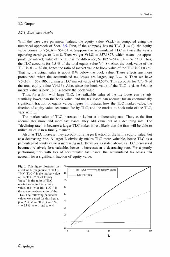
significant fraction of equity value. Figure 1 illustrates how the TLC market value, the

fraction of equity value accounted for by TLC, and the market-to-book ratio of the TLC,

vary with L.

The market value of TLC increases in L, but at a decreasing rate. Thus, as the firm

accumulates more and more tax losses, they add value but at a declining rate. The

‘‘declining rate’’ is because a larger TLC makes it less likely that the firm will be able to

utilize all of it in a timely manner.

Also, as TLC increase, they account for a larger fraction of the firm’s equity value, but

at a decreasing rate. A larger L obviously makes TLC more valuable, hence TLC as a

percentage of equity value is increasing in L. However, as stated above, as TLC increases it

becomes relatively less valuable, hence it increases at a decreasing rate. For a poorly

performing firm with lots of accumulated tax losses, the accumulated tax losses can

account for a significant fraction of equity value.

0

1

2

3

4

5

6

7

8

9

0 5 10 15 20

L

MV(TLC) % of Equity Value

Mkt-Bk(TLC)

Fig. 1 This figure illustrates theeffect of L (magnitude of TLC).‘‘MV (TLC)’’ is the market valueof the TLC, ‘‘ % of EquityValue’’ is the ratio of TLCmarket value to total equityvalue, and ‘‘Mkt-Bk (TLC)’’ isthe market-to-book ratio of theTLC. The following parametervalues were used for this figure:l = 2 %, r = 30 %, r = 6 %,s = 35 %, c = 1 and x = 4

S. Sarkar

123

Finally, the market-to-book ratio of the TLC is a decreasing function of the amount of

TLC, for the same reason stated above. For large TLC, the market value can be signifi-

cantly below the book value, i.e., a significant fraction of the tax losses might go

unrealized.

3.2.2 Comparative static results

The comparative static results are summarized in Table 1. The market value (hence the

market-to-book ratio) of the TLC is an increasing function of the earnings growth rate l. If

earnings are expected to grow faster, the firm can expect greater utilization of the tax losses

in a timely manner, hence they become more valuable. However, the ratio of market value

of TLC to the firm’s equity value is a decreasing function of l, because the equity value

rises faster than the TLC value. For a firm with low growth rate and large TLC, tax losses

account for a significant fraction of the total equity value; in our example, with l = 0 and

L = 12 (or three years’ earnings), tax losses account for almost 10 % of total equity value.

The effect of earnings volatility r on the market value (hence the market-to-book ratio)

of the TLC is ambiguous. For small TLC (in our example, for L = 4 and 8), it is increasing

in r, but for larger TLC (here L = 12), it is decreasing in r. Earnings volatility has a

similar effect on the ratio of market value of TLC to total equity value; for L = 4 it is

slightly increasing in r, for L = 8 and 12, it is decreasing in r. When volatility is

increased, there are two effects. On one hand, the bankruptcy trigger xd falls (a standard

result from option theory); this reduces bankruptcy risk and therefore increases the value of

the TLC. On the other hand, a higher r means that x is more likely to reach extreme levels

(both high and low), and this increases bankruptcy risk and therefore reduces TLC value.

The overall effect of volatility is therefore ambiguous.

The market value (hence the market-to-book ratio) of the TLC is a decreasing function

of r. With higher interest rate, the future benefits from the tax losses will be smaller on a

present-value basis, thus the TLC value will be lower. However, the ratio of TLC value to

equity value rises as the interest rate is increased, because equity value is more sensitive to

interest rate, hence it falls by a larger margin than the TLC value.

As mentioned in Sect. 2.1, there is also some statutory progressivity in the tax code,

since very small profits (below $100,000) are taxed at a lower rate (15 % instead of 34 %).

If this statutory progressivity is taken into account, the actual tax rate might be a little

smaller than the maximum statutory rate. To incorporate this possibility, we repeated the

numerical computations with smaller tax rates, i.e., s = 15 and 25 %. As evident from

Table 1, the results are as expected. For smaller tax rate, the market value of TLC declines;

also, the relative importance of TLC as a source of value (i.e., the ratio MV(TLC)/Total

Equity Value) declines as the tax rate is lowered.

Finally, we are also interested in the role of leverage in the determination of TLC value;

we expect that it will be worth less to high-leverage companies than to low-leverage

companies. We therefore repeated the numerical computations with different leverage

ratios (by varying x, with higher x representing lower leverage ratio and lower x repre-

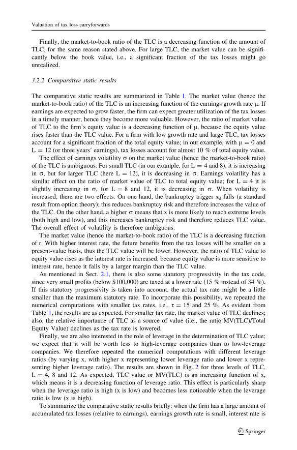
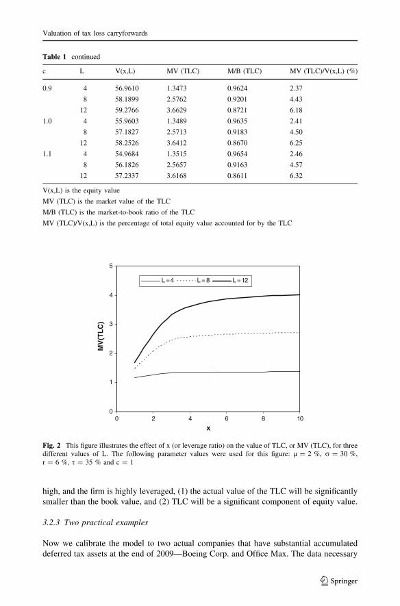
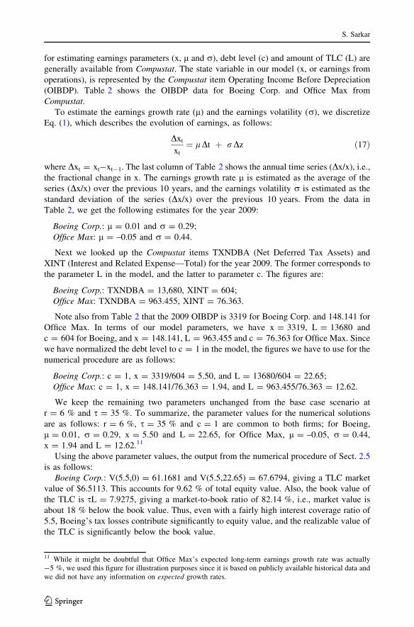
senting higher leverage ratio). The results are shown in Fig. 2 for three levels of TLC,

L = 4, 8 and 12. As expected, TLC value or MV(TLC) is an increasing function of x,

which means it is a decreasing function of leverage ratio. This effect is particularly sharp

when the leverage ratio is high (x is low) and becomes less noticeable when the leverage

ratio is low (x is high).

To summarize the comparative static results briefly: when the firm has a large amount of

accumulated tax losses (relative to earnings), earnings growth rate is small, interest rate is


123

Table 1 Comparative static results

Base case parameter values: l = 2 %, r = 30 %, r = 6 %, s = 35 %, c = 1, and x = 4.

l L V(x,L) MV (TLC) M/B (TLC) MV (TLC)/V(x,L) (%)

0 4 34.8949 1.3408 0.9577 3.84

8 36.0904 2.5363 0.9058 7.03

12 37.1161 3.5620 0.8481 9.60

2 % 4 55.9603 1.3489 0.9635 2.41

8 57.1827 2.5713 0.9183 4.50

12 58.2526 3.6412 0.8670 6.25

4 % 4 120.5219 1.3528 0.9663 1.12

8 121.7600 2.5909 0.9253 2.13

12 122.8596 3.6905 0.8787 3.00

r L V(x,L) MV (TLC) M/B (TLC) MV (TLC)/V(x,L) (%)

0.2 4 55.5560 1.3391 0.9565 2.41

8 56.7858 2.5689 0.9175 4.52

12 57.9051 3.6882 0.8781 6.37

0.3 4 55.9603 1.3489 0.9635 2.41

8 57.1827 2.5713 0.9183 4.50

12 58.2526 3.6412 0.8670 6.25

0.4 4 56.7201 1.3747 0.9819 2.42

8 57.9195 2.5741 0.9193 4.44

12 58.9142 3.5688 0.8497 6.06

r L V(x,L) MV (TLC) M/B (TLC) MV (TLC)/V(x,L) (%)

5 % 4 75.6386 1.3664 0.9760 1.81

8 76.9055 2.6333 0.9405 3.42

12 78.0332 3.7610 0.8955 4.82

6 % 4 55.9603 1.3489 0.9635 2.41

8 57.1827 2.5713 0.9183 4.50

12 58.2526 3.6412 0.8670 6.25

7 % 4 44.3820 1.3341 0.9529 3.01

8 45.5671 2.5192 0.8997 5.53

12 46.5882 3.5403 0.8429 7.60

s L V(x,L) MV (TLC) M/B (TLC) MV (TLC)/V(x,L) (%)

15 % 4 72.1131 0.5967 0.9945 0.83

8 72.6764 1.1600 0.9667 1.60

12 73.1730 1.6566 0.9203 2.26

25 % 4 64.0347 0.9728 0.9728 1.52

8 64.9277 1.8658 0.9329 2.87

12 65.7112 2.6493 0.8831 4.03

35 % 4 55.9603 1.3489 0.9635 2.41

8 57.1827 2.5713 0.9183 4.50

12 58.2526 3.6412 0.8670 6.25

S. Sarkar

123

high, and the firm is highly leveraged, (1) the actual value of the TLC will be significantly

smaller than the book value, and (2) TLC will be a significant component of equity value.

3.2.3 Two practical examples

Now we calibrate the model to two actual companies that have substantial accumulated

deferred tax assets at the end of 2009—Boeing Corp. and Office Max. The data necessary

0

1

2

3

4

5

0 2 4 6 8 10

x

MV

(TL

C)

L = 4 L = 8 L = 12

Fig. 2 This figure illustrates the effect of x (or leverage ratio) on the value of TLC, or MV (TLC), for threedifferent values of L. The following parameter values were used for this figure: l = 2 %, r = 30 %,r = 6 %, s = 35 % and c = 1

Table 1 continued

c L V(x,L) MV (TLC) M/B (TLC) MV (TLC)/V(x,L) (%)

0.9 4 56.9610 1.3473 0.9624 2.37

8 58.1899 2.5762 0.9201 4.43

12 59.2766 3.6629 0.8721 6.18

1.0 4 55.9603 1.3489 0.9635 2.41

8 57.1827 2.5713 0.9183 4.50

12 58.2526 3.6412 0.8670 6.25

1.1 4 54.9684 1.3515 0.9654 2.46

8 56.1826 2.5657 0.9163 4.57

12 57.2337 3.6168 0.8611 6.32

V(x,L) is the equity value

MV (TLC) is the market value of the TLC

M/B (TLC) is the market-to-book ratio of the TLC

MV (TLC)/V(x,L) is the percentage of total equity value accounted for by the TLC


123

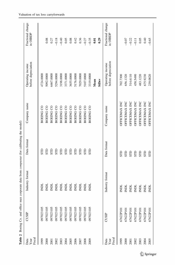
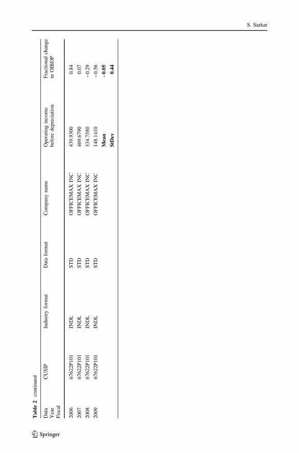
for estimating earnings parameters (x, l and r), debt level (c) and amount of TLC (L) are

generally available from Compustat. The state variable in our model (x, or earnings from

operations), is represented by the Compustat item Operating Income Before Depreciation

(OIBDP). Table 2 shows the OIBDP data for Boeing Corp. and Office Max from

Compustat.

To estimate the earnings growth rate (l) and the earnings volatility (r), we discretize

Eq. (1), which describes the evolution of earnings, as follows:

Dxt

xt

¼ l Dt þ r Dz ð17Þ

where Dxt = xt-xt-1. The last column of Table 2 shows the annual time series (Dx/x), i.e.,

the fractional change in x. The earnings growth rate l is estimated as the average of the

series (Dx/x) over the previous 10 years, and the earnings volatility r is estimated as the

standard deviation of the series (Dx/x) over the previous 10 years. From the data in

Table 2, we get the following estimates for the year 2009:

Boeing Corp.: l = 0.01 and r = 0.29;

Office Max: l = –0.05 and r = 0.44.

Next we looked up the Compustat items TXNDBA (Net Deferred Tax Assets) and

XINT (Interest and Related Expense—Total) for the year 2009. The former corresponds to

the parameter L in the model, and the latter to parameter c. The figures are:

Boeing Corp.: TXNDBA = 13,680, XINT = 604;

Office Max: TXNDBA = 963.455, XINT = 76.363.

Note also from Table 2 that the 2009 OIBDP is 3319 for Boeing Corp. and 148.141 for

Office Max. In terms of our model parameters, we have x = 3319, L = 13680 and

c = 604 for Boeing, and x = 148.141, L = 963.455 and c = 76.363 for Office Max. Since

we have normalized the debt level to c = 1 in the model, the figures we have to use for the

numerical procedure are as follows:

Boeing Corp.: c = 1, x = 3319/604 = 5.50, and L = 13680/604 = 22.65;

Office Max: c = 1, x = 148.141/76.363 = 1.94, and L = 963.455/76.363 = 12.62.

We keep the remaining two parameters unchanged from the base case scenario at

r = 6 % and s = 35 %. To summarize, the parameter values for the numerical solutions

are as follows: r = 6 %, s = 35 % and c = 1 are common to both firms; for Boeing,

l = 0.01, r = 0.29, x = 5.50 and L = 22.65, for Office Max, l = –0.05, r = 0.44,

x = 1.94 and L = 12.62.11

Using the above parameter values, the output from the numerical procedure of Sect. 2.5

is as follows:

Boeing Corp.: V(5.5,0) = 61.1681 and V(5.5,22.65) = 67.6794, giving a TLC market

value of $6.5113. This accounts for 9.62 % of total equity value. Also, the book value of

the TLC is sL = 7.9275, giving a market-to-book ratio of 82.14 %, i.e., market value is

about 18 % below the book value. Thus, even with a fairly high interest coverage ratio of

5.5, Boeing’s tax losses contribute significantly to equity value, and the realizable value of

the TLC is significantly below the book value.

11 While it might be doubtful that Office Max’s expected long-term earnings growth rate was actually-5 %, we used this figure for illustration purposes since it is based on publicly available historical data andwe did not have any information on expected growth rates.

S. Sarkar

123

Ta

ble

2B

oei

ng

Co.

and

offi

cem

axco

rpo

rate

dat

afr

om

com

pu

sta

t(f

or

cali

bra

tin

gth

em

od

el)

Dat

aY

ear

Fis

cal

CU

SIP

Ind

ust

ryfo

rmat

Dat

afo

rmat

Co

mpan

yn

ame

Op

erat

ing

inco

me

bef

ore

dep

reci

atio

nF

ract

ional

chan

ge

inO

IBD

P

19

99

09

702

31

05

IND

LS

TD

BO

EIN

GC

O4

72

4.0

000

20

00

09

702

31

05

IND

LS

TD

BO

EIN

GC

O5

09

2.0

000

0.0

8

20

01

09

702

31

05

IND

LS

TD

BO

EIN

GC

O6

46

7.0

000

0.2

7

20

02

09

702

31

05

IND

LS

TD

BO

EIN

GC

O5

29

4.0

000

-0

.18

20

03

09

702

31

05

IND

LS

TD

BO

EIN

GC

O3

19

8.0

000

-0

.40

20

04

09

702

31

05

IND

LS

TD

BO

EIN

GC

O3

37

1.0

000

0.0

5

20

05

09

702

31

05

IND

LS

TD

BO

EIN

GC

O3

65

5.0

000

0.0

8

20

06

09

702

31

05

IND

LS

TD

BO

EIN

GC

O5

17

6.0

000

0.4

2

20

07

09

702

31

05

IND

LS

TD

BO

EIN

GC

O7

02

9.0

000

0.3

6

20

08

09

702

31

05

IND

LS

TD

BO

EIN

GC

O5

10

7.0

000

-0

.27

20

09

09

702

31

05

IND

LS

TD

BO

EIN

GC

O3

31

9.0

000

-0

.35

Mea

n0

.01

StD

ev0

.29

Dat

aY

ear

Fis

cal

CU

SIP

Ind

ust

ryfo

rmat

Dat

afo

rmat

Co

mpan

yn

ame

Op

erat

ing

inco

me

bef

ore

dep

reci

atio

nF

ract

ional

chan

ge

inO

IBD

P

19

99

67

622

P1

01

IND

LS

TD

OF

FIC

EM

AX

INC

70

2.7

30

0

20

00

67

622

P1

01

IND

LS

TD

OF

FIC

EM

AX

INC

65

6.1

32

0-

0.0

7

20

01

67

622

P1

01

IND

LS

TD

OF

FIC

EM

AX

INC

51

4.6

11

0-

0.2

2

20

02

67

622

P1

01

IND

LS

TD

OF

FIC

EM

AX

INC

45

8.5

49

0-

0.1

1

20

03

67

622

P1

01

IND

LS

TD

OF

FIC

EM

AX

INC

48

3.1

22

00

.05

20

04

67

622

P1

01

IND

LS

TD

OF

FIC

EM

AX

INC

67

5.9

23

00

.40

20

05

67

622

P1

01

IND

LS

TD

OF

FIC

EM

AX

INC

23

9.0

82

0-

0.6

5


123

Ta

ble

2co

nti

nued

Dat

aY

ear

Fis

cal

CU

SIP

Ind

ust

ryfo

rmat

Dat

afo

rmat

Co

mpan

yn

ame

Op

erat

ing

inco

me

bef

ore

dep

reci

atio

nF

ract

ional

chan

ge

inO

IBD

P

20

06

67

622

P1

01

IND

LS

TD

OF

FIC

EM

AX

INC

43

9.9

30

00

.84

20

07

67

622

P1

01

IND

LS

TD

OF

FIC

EM

AX

INC

46

9.6

79

00

.07

20

08

67

622

P1

01

IND

LS

TD

OF

FIC

EM

AX

INC

33

4.7

58

0-

0.2

9

20

09

67

622

P1

01

IND

LS

TD

OF

FIC

EM

AX

INC

14

8.1

41

0-

0.5

6

Mea

n-

0.0

5

StD

ev0

.44

S. Sarkar

123

Office Max: V(1.94,0) = 5.5504 and V(1.94,12.62) = 7.0963, giving a TLC market

value of $1.5459. Thus, tax losses account for a substantial 21.78 % of total equity value.

The book value of the TLC is sL = 4.4170, giving a market-to-book ratio of only 35 %,

i.e., market value is 65 % below book value.

As discussed in footnote 5, l = -0.05 probably reflects a period of temporary negative

earnings growth rather than a long-term trend. We therefore repeated the calculations with

zero growth rate (l = 0) and get the following results: V(1.94,0) = 13.3317,

V(1.94,12.62) = 15.7260, TLC market value of $2.3943, which accounts for 15.23 % of

total equity value, and has a market-to-book ratio of 54.21 %. Even with zero growth rate

(instead of -5 %), TLC accounts for a substantial fraction of equity value and is worth a

lot less than the book value. This is because of (1) the low earnings level relative to the

debt level (interest coverage ratio \2), which can also be viewed as high leverage ratio,

and (2) large TLC relative to the earnings level.

3.2.4 Historical versus forward-looking parameter values

Note that our above calibration and estimation of input parameters for the two companies

was based entirely on publicly available historical data. However, the parameter values

should actually be forward-looking estimates. This is because the value of the TLC

depends on the future utilization of these tax shields, hence the valuation should be

contingent on future cash flows.

Thus, in order to get the appropriate estimates, the historical data will have to be adjusted for

changes that are expected to take place. If, for instance, the company expects increased

uncertainty in the future (more volatile cash flows), then the volatility used in the computations

should reflect the higher volatility expected in the future rather than the lower volatility

observed in the past. These adjustments in parameter values can be made by the company’s

managers and/or other informed insiders. Unfortunately, making such adjustments is difficult

for outsiders, since only the company’s top management would have the kind of information

(possibly inside information) necessary to make such adjustments. Therefore, our valuation of

Boeing’s and Office Max’s TLC is subject to the caveat that it is based on historical (and not

necessarily forward-looking) estimates. In practice, our model’s results would be more reli-

able with forward-looking rather than historical estimates of the input parameters.

3.2.5 Market valuation vis-a-vis model valuation

We next compare the equity value from the model with the market equity value. Our

calculations are based on c = 1, while the actual values are c = 604 for Boeing and

c = 76.363 for Office Max. Therefore, the model’s valuation of Boeing’s equity at end-

2009 would be (67.6794 9 604) = $40,878.36 million; and Office Max’s equity value

would be (7.0963 9 76.363) = $541.89 million.

From Compustat, we also get the following market-value information for end-2009: the

number of shares was 726.69 million for Boeing and 76.293 million for Office Max, and

the year-end share price was $54.13 for Boeing and $12.69 for Office Max. The market

valuation is just the product of number of shares and share price, giving $39,335.73 million

for Boeing and $968.16 million for Office Max. Comparing the model valuation with the

market valuation, we see that the two are very close (a difference of 3.9 %) for Boeing

Corp., but very different for Office Max. The market valuation of Office Max is signifi-

cantly higher (almost 79 %) than the model’s valuation. One reason could be that the

earnings growth rate expected by the market was higher than the -5 % we had used (based


123

on the last 10 years of earnings growth data). This shows the importance of making

appropriate adjustments to the raw historical estimates of the parameters (i.e., using for-

ward-looking parameter estimates), a common problem in the use of any valuation model.

3.2.6 Valuation for a Sample of Compustat Firms

We repeated the above valuation exercise for a sample of 30 firms in the Compustat

database from a variety of industries. For this broader sample, we use the same calibration

procedure as the two firms above (Boeing and Office Max), so the detailed description of

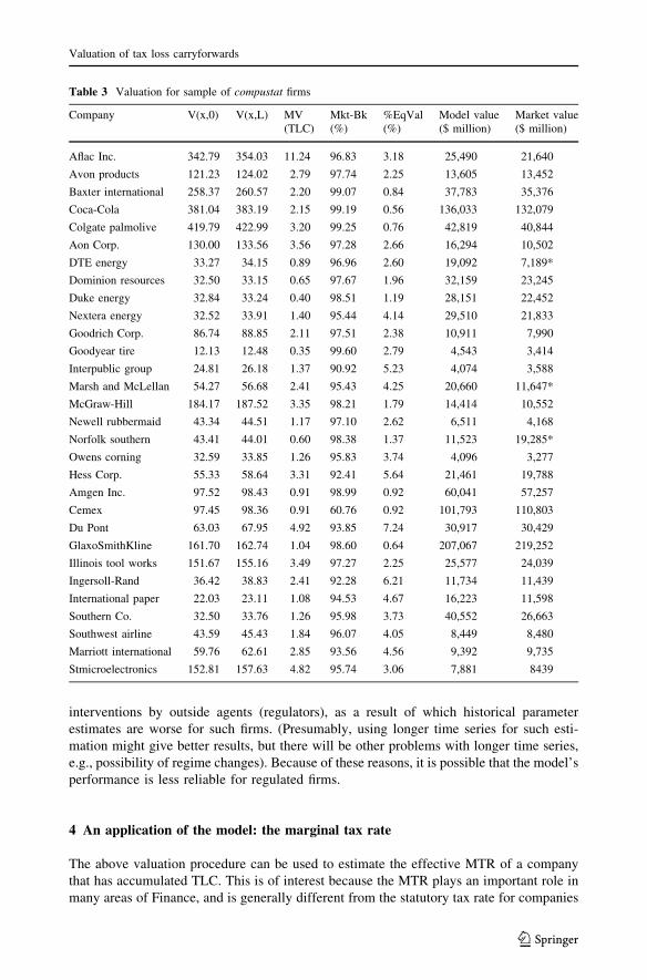
the calibration is not repeated here. The results are summarized in Table 3. It is clear from

the results that the value of the TLC, relative to its book value, varies considerably across

firms, form a low of 61 % to a high of 99 %. The TLC value as a fraction of total equity

value also varies widely, from 0.56 to 7.24 %. Thus, there seems to be wide dispersion in

the valuation of TLC, even in a relatively small sample of 30 firms.

Table 3 also shows (the last two columns) the model-generated equity value and the

market-determined equity value for the sample of 30 firms. It is again clear that there is wide

dispersion in the results; for some firms, the model’s valuation is very close to the market

valuation while for other firms the two valuations are very far apart, with the model in one

case over-estimating equity value by over 100 % relative to market value. However, it is not

surprising that there are differences between model and market values, because the parameter

values in our calibration were not forward-looking, since we do not have either inside

information or market expectations regarding these parameter values. On the other hand,

market values are based on forward-looking market-consensus values.12 Thus, as stated in the

section above (Historical versus Forward-looking Parameter Values), the best way to apply

the model is to use forward-looking rather than historical estimates for the input parameters.

Looking at the equity value comparison (model versus market) in Table 3 in more

detail, we note that the difference is particularly large (over 60 %) for the three companies

market by an asterisk: DTE Energy, Marsh & McLellan and Norfolk Southern (difference

of 165, 77 and 67 % respectively). While these companies are in different industries (DTE

in utilities, M&M in insurance, and Norfolk Southern in railways), the one thing they have

in common is that they are all in regulated industries. This seems to suggest that the model

is less useful in valuing the firm’s equity for regulated industries.13 However, we have to be

careful about reaching any firm conclusions because it is s small sample and a cursory

comparison, not a rigorous empirical study.

Nevertheless, it might seem surprising that the model seems to be less useful for

regulated industries, because regulated industries tend to be more stable in the long run,

since regulators generally act to compensate for any large unexpected changes in the

marketplace. We can try to explain it intuitively as follows. In one sense, regulators add to

parameter value uncertainty in the short run by intervening in the market, in two ways, (1)

the market does not know when the intervention will occur, and this increases uncertainty,

and (2) market intervention results in changes in the short-run estimates of parameter

values. Thus, under regulation, future performance is more subject to uncertain

12 A rigorous empirical study could, of course, use market (analyst) expectations, if available, to comparemodel and market values to examine the usefulness of the model. However, such a study is beyond the scopeof our paper.13 Note that our main objective is to value TLC and not the value of the firm’s equity. However, TLC arenot traded, making it very difficult to evaluate the model’s performance. Therefore, to check for model’sreliability, we look at model versus market values for equity, since the equity market values are available.

S. Sarkar

123

interventions by outside agents (regulators), as a result of which historical parameter

estimates are worse for such firms. (Presumably, using longer time series for such esti-

mation might give better results, but there will be other problems with longer time series,

e.g., possibility of regime changes). Because of these reasons, it is possible that the model’s

performance is less reliable for regulated firms.

4 An application of the model: the marginal tax rate

The above valuation procedure can be used to estimate the effective MTR of a company

that has accumulated TLC. This is of interest because the MTR plays an important role in

many areas of Finance, and is generally different from the statutory tax rate for companies

Table 3 Valuation for sample of compustat firms

Company V(x,0) V(x,L) MV(TLC)

Mkt-Bk(%)

%EqVal(%)

Model value($ million)

Market value($ million)

Aflac Inc. 342.79 354.03 11.24 96.83 3.18 25,490 21,640

Avon products 121.23 124.02 2.79 97.74 2.25 13,605 13,452

Baxter international 258.37 260.57 2.20 99.07 0.84 37,783 35,376

Coca-Cola 381.04 383.19 2.15 99.19 0.56 136,033 132,079

Colgate palmolive 419.79 422.99 3.20 99.25 0.76 42,819 40,844

Aon Corp. 130.00 133.56 3.56 97.28 2.66 16,294 10,502

DTE energy 33.27 34.15 0.89 96.96 2.60 19,092 7,189*

Dominion resources 32.50 33.15 0.65 97.67 1.96 32,159 23,245

Duke energy 32.84 33.24 0.40 98.51 1.19 28,151 22,452

Nextera energy 32.52 33.91 1.40 95.44 4.14 29,510 21,833

Goodrich Corp. 86.74 88.85 2.11 97.51 2.38 10,911 7,990

Goodyear tire 12.13 12.48 0.35 99.60 2.79 4,543 3,414

Interpublic group 24.81 26.18 1.37 90.92 5.23 4,074 3,588

Marsh and McLellan 54.27 56.68 2.41 95.43 4.25 20,660 11,647*

McGraw-Hill 184.17 187.52 3.35 98.21 1.79 14,414 10,552

Newell rubbermaid 43.34 44.51 1.17 97.10 2.62 6,511 4,168

Norfolk southern 43.41 44.01 0.60 98.38 1.37 11,523 19,285*

Owens corning 32.59 33.85 1.26 95.83 3.74 4,096 3,277

Hess Corp. 55.33 58.64 3.31 92.41 5.64 21,461 19,788

Amgen Inc. 97.52 98.43 0.91 98.99 0.92 60,041 57,257

Cemex 97.45 98.36 0.91 60.76 0.92 101,793 110,803

Du Pont 63.03 67.95 4.92 93.85 7.24 30,917 30,429

GlaxoSmithKline 161.70 162.74 1.04 98.60 0.64 207,067 219,252

Illinois tool works 151.67 155.16 3.49 97.27 2.25 25,577 24,039

Ingersoll-Rand 36.42 38.83 2.41 92.28 6.21 11,734 11,439

International paper 22.03 23.11 1.08 94.53 4.67 16,223 11,598

Southern Co. 32.50 33.76 1.26 95.98 3.73 40,552 26,663

Southwest airline 43.59 45.43 1.84 96.07 4.05 8,449 8,480

Marriott international 59.76 62.61 2.85 93.56 4.56 9,392 9,735

Stmicroelectronics 152.81 157.63 4.82 95.74 3.06 7,881 8439


123

with TLC (Graham 1996a). Our procedure is somewhat similar to Shevlin (1990) and

Graham (1996a, b), in that we also incorporate earnings uncertainty by using a specific

stochastic process, and the MTR is based on expected future outcomes of the random

earnings process. However, these papers use a random walk process while we use a

lognormal process; also, we solve a partial differential equation, while Shevlin (1990) and

Graham (1996a, b) simulate a large number of earnings paths and take the average.

Shevlin (1990) and Graham (1996a, b) estimate the MTR by increasing the current

earnings by a dollar and computing the present value of all (including future) resulting tax

payments. Since ours is a valuation model, our estimation of the MTR is based on values.

We increase current earnings x by a small increment Dx (which will also have a ripple

effect on future earnings realizations) and compute the increase in value. Comparing this to

the value increase in a tax-free world, we extract the implied MTR of the firm. The exact

procedure is as follows:

1. first, the equity value V(x,L) is computed as above;

2. next, the earnings figure x is increased by an incremental amount Dx, and the new

equity value V(x ? Dx,L) computed;

3. the difference between the two figures gives the after-tax value of the incremental

earnings stream, [V(x ? Dx,L) - V(x,L)];

4. the value added by the same earnings increment Dx in a tax-free world is computed

using E(x|s = 0), the equity value (from Appendix 2) in a world without taxation;

thus, the value of the incremental earnings stream in a tax-free world is given by

[E(x ? Dx |s = 0) - E(x|s = 0)]; and

5. comparing the after-tax value added with the value added in a tax-free world, we can

extract the implied Marginal Tax Rate, given by:

MTR = 1 - [Value added (taxable)/Value added (tax-free)].

4.1 MTRs for Boeing and Office Max for 2009

Here we illustrate the procedure for computing MTR, for the two companies examined

above. Using Dx = 1 % of x, we have:

Boeing Co.: V(5.5,22.65) = 67.6794 and V(5.5*1.01,22.65) = 67.8123. The after-tax

value of the incremental earnings stream is the difference $0.1329. The pre-tax value of

the earnings stream (or its value in a tax-free world) is given by [E(5.5*1.01|s = 0) -

E(5.5|s = 0)] = 94.4124 - 94.2138 = $0.1986. Then the implied (or effective) MTR is

given by [1 - (0.1329/0.1986)] = 33.08 %. Thus, even with fairly large earnings (i.e.,

interest coverage ratio of 5.5), the MTR is lowered somewhat (relative to the statutory rate

of 35 %) by the presence of the accumulated tax losses.

Office Max: V(1.94,12.62) = 7.0963 and V(1.94*1.01,12.62) = 7.1591. The after-tax value of

the incremental earnings stream is the difference $0.0628. The pre-tax value of the earnings stream

(or its value in a tax-free world) is given by [E(1.94*1.01|s = 0) - E(1.94|s = 0)] = 8.7584 -

8.6808 = $0.0776. Then the implied (or effective) MTR is given by [1 - (0.0628/

0.0776)] = 19.07 %. In this case, because of the smaller earnings (coverage ratio\2) and the large

tax losses, the MTR is significantly lower than the statutory rate of 35 %.

4.2 MTR estimates for a sample of compustat firms

Using the above procedure for estimating MTRs, we repeat the computations for the

sample of 30 Compustat firms from Sect. 3.2, and summarize the results in Table 4 (note

S. Sarkar

123

that four of the 30 firms are dropped because Compustat MTR estimates are not available,

hence the sample size is down to 26). As we can see from Table 4, there is considerable

variation in the estimated MTRs, with values ranging from 16 to 35 %. For comparison, we

Table 4 MTR estimates for sample of compustat firms

Company Taxable world Non-taxable world ModelMTR (%)

CompustatMTR (%)

V(x,L) V(x ? dx,L) DV V(x,L) V(x ? dx,L) DV

Aflac Inc. 354.03 357.57 3.54 527.37 532.28 4.91 27.90 29.60

Avonproducts

124.02 125.35 1.33 186.52 188.55 2.03 34.48 33.47

Baxterinternational

260.58 263.27 2.69 397.50 401.63 4.13 34.87 33.75

Coca-Cola 383.19 387.11 3.92 586.22 592.11 5.89 33.45 34.3

Colgatepalmolive

422.99 427.30 4.31 645.83 652.44 6.61 34.80 33.28

Aon Corp. 133.56 135.01 1.45 200.00 202.17 2.17 33.18 33.28

DTE energy 34.15 34.64 0.49 51.21 51.84 0.63 22.22 21.70

Dominionresources

33.15 33.58 0.43 50.01 50.67 0.66 34.85 35.00

Duke energy 33.24 33.72 0.48 50.59 51.21 0.62 22.58 18.74

Nexteraenergy

33.92 34.38 0.46 50.03 50.69 0.66 30.30 29.80

GoodrichCorp.

88.85 89.86 1.01 133.45 134.95 1.50 32.67 30.69

Goodyear tire 12.48 12.72 0.24 18.83 19.13 0.30 20.00 15.99

Interpublicgroup

26.18 26.56 0.38 38.52 39.00 0.48 20.83 14.94

Marsh &McLellan

56.68 57.35 0.67 83.50 84.50 1.00 33.00 31.97

McGraw-Hill 187.52 189.48 1.96 283.33 286.33 3.00 34.67 34.30

NewellRubbermaid

44.51 45.06 0.55 66.68 67.51 0.83 33.73 32.03

NorfolkSouthern

44.01 44.58 0.57 66.80 67.63 0.83 31.33 30.75

Owenscorning

33.85 34.38 0.53 50.15 50.79 0.64 17.19 6.28

Hess Corp. 58.64 59.29 0.65 85.26 86.25 0.99 34.34 34.77

Amgen Inc. 98.43 99.53 1.10 150.04 151.70 1.66 33.73 33.60

Du pont 73.06 73.87 0.81 104.81 105.99 1.18 31.36 29.40

Illinois toolworks

211.03 213.25 2.22 319.30 322.65 3.35 33.73 33.93

Internationalpaper

36.44 36.99 0.55 54.40 55.11 0.71 22.54 18.08

Southern Co. 83.70 84.64 0.94 126.81 128.24 1.43 34.27 32.90

Southwestairline

54.23 54.86 0.63 80.65 81.62 0.97 35.00 35.00

MarriottInternational

89.02 90.03 1.01 132.66 134.15 1.49 32.21 33.47


123

have also listed the MTR estimates in Compustat (these estimates were developed by

Blouin et al. 2010). These are arguably the most well-established MTR estimates, and are

based on a rigorous empirical study using a non-parametric process to simulate the future

earnings stream.

It can be noted from Table 4 that there are differences between our estimates and the

Compustat estimates. One reason is that ours is a value-based estimate while the other is

earnings-based (as discussed above, we estimate MTR form the ratio of values of the

marginal dollar earned with and without taxes). Moreover, our estimates do not use for-

ward-looking parameter values, since they are just to illustrate the model’s application and

not a full-fledged empirical study. Nevertheless, our model suggests an alternative method

to compute MTRs, whose performance should improve if using forward-looking parameter

values. However, that is beyond the scope of the present study and is left for future

research.

5 Summary and conclusion

This paper uses a contingent-claim model to value the accumulated TLC of a company.

The model incorporates earnings volatility, the resulting random changes in the amount of

TLC, and the possibility of bankruptcy. The fair (or realizable) value of the TLC is derived

as a function of the level, growth rate and volatility of earnings, amount of carryforwards,

debt level, interest rate and tax rate. Because of the complexity of the model, it has to be

solved numerically.

The model is illustrated by calibrating it to a couple of companies with large TLC. It is

shown that, for poorly performing companies with large TLC, (1) the realizable value of

the TLC can be substantially below the book value, and (2) the TLC can make a significant

contribution to company’s equity value. We also illustrate how the model can be used to

compute the MTR of a company with TLC.

The input parameter values were assumed to be known in the numerical computations

(historical data were used for calibration purposes). However, when using the model in real

life, we would likely be confronted by the problem of coming up with appropriate forward-

looking estimates of these parameters (particularly the firm-specific parameters such as

earnings growth rate and volatility). These parameter values should ideally incorporate all

relevant information about future performance (including private information available

only to insiders), as in all valuation models.

In developing the model and implementing the numerical solution, we had to make a

few simplifying assumptions, i.e., TLC does not expire, default risk is zero at x = xMax,

default trigger is independent of amount of TLC, and ignoring the possibility that there

might be TLC in the future when current TLC falls to zero. However, as pointed out

earlier, these assumptions are not entirely unrealistic. Moreover, the first two assumptions

cause the model to overstate, while the other two assumptions cause the model to

understate, the value of the TLC; thus, there will be some cancelling-out effect, and the net

effect of these simplifying assumptions should not be significant. Thus, even with the

simplifying assumptions, the model should give us a reasonable first approximation.

Acknowledgments Financial support from the Social Science and Humanities Research Council (SSHRC)of Canada is gratefully acknowledged. I would like to thank two anonymous referees for their helpfulcomments and suggestions, and the Editor C.F. Lee for his recommendations during the review process. Theusual disclaimer applies.

S. Sarkar

123

Appendix 1: derivations of equations in Sect. 2.3

Equation (2): Region I [L [ 0, cash flow to shareholders = (x-c) per unit time, and

dL = (c - x) dt].

Equity value = V(x,L). From Ito’s lemma, we have: dV ¼ Vxdx þ 0:5 Vxx dxð Þ2þVLdL (the other terms drop out because (dt)2 = 0, (dL)2 = 0, and (dt dL) = 0).

We know dx ¼ lx dt þ rx dz, from Eq. (1); also, dL = (c - x) dt. Substituting for dx

and dL, we get

dV ¼ Vx lx dt þ rx dzð Þ þ 0:5 Vxx r2x2dt� �

þ VL c� xð Þ dt:

Taking expectations (and keeping in mind that E(dz) = 0), we get:

E dVð Þ ¼ Vxlx þ 0:5 Vxx r2x2� �

þ VL c� xð Þ� �

dt:

This is the expected capital gain over an incremental period of time dt. In addition, there

is a dividend of (x - c)dt, over this time period. Thus, the total instantaneous return is

lx Vx þ 0:5r2x2 Vxx þ ðc� xÞVL þ ðx� cÞV

:

From the Local Expectations Hypothesis, this should be equal to the risk-free rate r, i.e.

lx Vx þ 0:5r2x2 Vxx þ ðc� xÞVL þ ðx� cÞ ¼ rV;

which is the partial differential Eq. (2) of the paper.

Equation (3): Region II [L = 0, cash flow to equity holders = (1 - s)(x - c) per unit

time, and dL = 0].

Equity value = U(x). Then we follow a procedure similar to the above.

From Ito’s lemma: dU ¼ Uxdxþ 0:5 Uxx dxð Þ2¼ U0 xð Þ lx dtþ rx dzð Þ þ 0:5 U00 xð Þr2x2dtð Þ.

Taking expectations: E(dU) = [U0(x) lx ? 0.5 U

00(x) (r2x2)] dt.

This is the expected capital gain over an incremental period of time dt. In addition, there

is a dividend of (1 - s)(x - c) dt over this time period. Thus, the total instantaneous

return is

lx U0ðxÞ þ 0:5r2x2 U00ðXÞ þ ð1� sÞðx� cÞU

From the Local Expectations Hypothesis, this should be equal to the risk-free rate r, i.e.

lx U0ðxÞ þ 0:5r2x2 U00ðXÞ þ ð1� sÞðx� cÞ ¼ rU;

which is the ODE (3) of the paper.

Equation (4).

The particular solution to ODE (3) is ð1� sÞ x=ðr� lÞ � c=r½ �, as can be verified by

direct substitution. The general solution to the ODE is U(x) = xc, which gives

U0(x) = cxc-1 and U00(x) = c(c - 1)xc-2. Substituting in the ODE and simplifying, we

get the quadratic equation: 0:5r2cðc� 1Þ þ lc� r ¼ 0, whose solutions are given by Eqs.

(6) and (7). Thus,

UðxÞ ¼ ð1� sÞ x=ðr� lÞ � c=r½ � þ Axc1 þ Bxc2 ð18ÞEquation (12): Smooth-pasting condition for the default trigger.


123

This requires that the derivative of V with respect to x (at default) equal the derivative

of the payoff. Since the payoff is zero, we get: Vx(xd(L),L) = 0.

Appendix 2: equity valuation when TLC are not allowed

In this case, no tax losses can be carried forward, hence there are no benefits associated

with losses; the tax rate is s for profits (x [ c) and zero for losses (x B c). The cash flow to

bondholders is $c per unit time until default, and the cash flow to equity holders is $(1 - s)

(x - c) per unit time if x [ c and $(x - c) if x B c, until default.

Thus, as far as equity holders are concerned, there are two operating regions: (1) Region

1 (profit region, or x [ c), with cash flow of (1 - s)(x - c) per unit time; and (2) Region 2

(loss region, or x B c), with cash flow of (x - c) per unit time.

Equity is a contingent claim (hence a function of x); and because of the perpetual setting

of the model, equity value will be time-independent; let the equity value be given by E(x).

Then, it can be shown as above that E(x) must satisfy the ODE:

0:5r2x2 E00ðxÞ þ lxE0ðxÞ � rEðxÞ þ 1ðxÞ ¼ 0 ð19Þ

where E0ðxÞ and E00ðxÞ represent first and second derivatives, and 1ðxÞ is the cash flow per

unit time to equity holders. The general solution to this ODE is14:

EðxÞ ¼ A1xc1 þ B1xc2 ð20Þ

where the constants A1 and B1 will be determined by boundary conditions, and c1 and c2

are given by Eqs. (6) and (7)

The cash flow to equity holders, 1ðxÞ, depends on the operating region; hence the equity

has to be valued separately for each operating region:

EðxÞ ¼ E1ðxÞ if x [ c

E2ðxÞ if x� c

ð21Þ

Region 1 (x [ c): Here, 1ðxÞ = (1 - s)(x - c). Solving ODE (19) with this 1ðxÞ, we

get the complete solution for the equity value:

E1ðxÞ ¼ ð1� sÞ x

r� l� c

r

� �þ A1xc1 þ B1xc2 ð22Þ


operating forever in Region 1. The other two terms reflect the effects of the boundary

x = c (moving to Region 2) and the boundary x ? ?. As x ? ?, the probability of

falling to Region 2 approaches zero, hence

E1ðxÞ ! ð1� sÞ x=ðr� lÞ � c=rð Þ ð23ÞThis implies A1 = 0 in equation (22), hence we write the equity value in Region 1 as:

E1ðxÞ ¼ ð1� sÞ x

r� l� c

r

� �þ B1xc2 ð24Þ

Region 2 (x B c): Here, 1ðxÞ = (x - c). Solving ODE (19) with this 1ðxÞ, we get the

complete solution for the equity value:

14 The particular solution will depend on the function 1(x).

S. Sarkar

123

E2ðxÞ ¼x

r� l� c

r

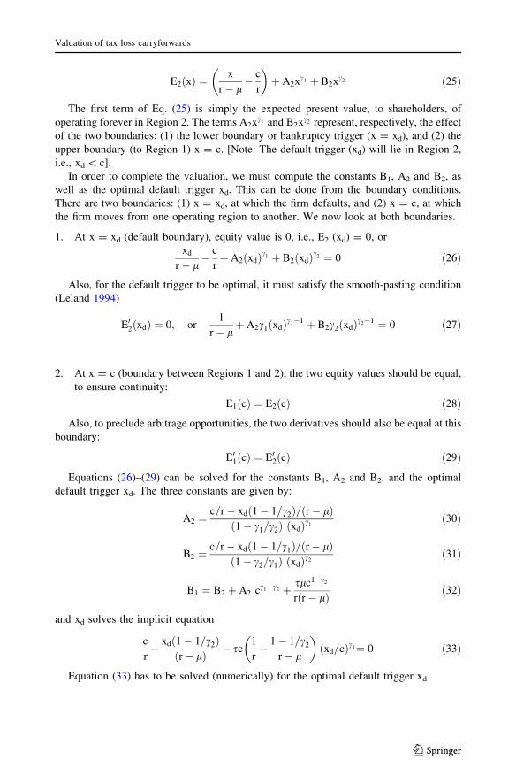
� �þ A2xc1 þ B2xc2 ð25Þ


operating forever in Region 2. The terms A2xc1 and B2xc2 represent, respectively, the effect

of the two boundaries: (1) the lower boundary or bankruptcy trigger (x = xd), and (2) the

upper boundary (to Region 1) x = c. [Note: The default trigger (xd) will lie in Region 2,

i.e., xd \ c].

In order to complete the valuation, we must compute the constants B1, A2 and B2, as

well as the optimal default trigger xd. This can be done from the boundary conditions.

There are two boundaries: (1) x = xd, at which the firm defaults, and (2) x = c, at which

the firm moves from one operating region to another. We now look at both boundaries.

1. At x = xd (default boundary), equity value is 0, i.e., E2 (xd) = 0, or

xd

r� l� c

rþ A2ðxdÞc1 þ B2ðxdÞc2 ¼ 0 ð26Þ

Also, for the default trigger to be optimal, it must satisfy the smooth-pasting condition

(Leland 1994)

E02ðxdÞ ¼ 0; or1

r� lþ A2c1ðxdÞc1�1 þ B2c2ðxdÞc2�1 ¼ 0 ð27Þ

2. At x = c (boundary between Regions 1 and 2), the two equity values should be equal,

to ensure continuity:

E1ðcÞ ¼ E2ðcÞ ð28ÞAlso, to preclude arbitrage opportunities, the two derivatives should also be equal at this

boundary:

E01ðcÞ ¼ E02ðcÞ ð29Þ

Equations (26)–(29) can be solved for the constants B1, A2 and B2, and the optimal

default trigger xd. The three constants are given by:

A2 ¼c=r� xdð1� 1=c2Þ=ðr� lÞð1� c1=c2Þ ðxdÞc1

ð30Þ

B2 ¼c=r� xdð1� 1=c1Þ=ðr� lÞð1� c2=c1Þ ðxdÞc2

ð31Þ

B1 ¼ B2 þ A2 cc1�c2 þ slc1�c2

rðr� lÞ ð32Þ

and xd solves the implicit equation

c

r� xdð1� 1=c2Þ

ðr� lÞ � sc1

r� 1� 1=c2

r� l

� �xd=cð Þc1¼ 0 ð33Þ

Equation (33) has to be solved (numerically) for the optimal default trigger xd.


123

References

Baez-Diaz A, Alam P (2013) Tax conformity of earnings and the pricing of accruals. Rev Quant FinancAccount 40(3):509–538

Bauman MP, Das S (2004) Stock market valuation of deferred tax assets: evidence from internet firms. J BusFinanc Account 31(9–10):1223–1260

Bhagat S, Moyen N, Suh I (2005) Investment and internal funds of distressed firms. J Corp Financ11(3):449–472

Blouin J, Core JE, Guay W (2010) Have the tax benefits of debt been overstated? J Financ Econ98(2):195–213

Broadie M, Chernov M, Sundaresan S (2007) Optimal dent and equity values in the presence of chapter 7and chapter 11. J Financ 62(3):1341–1377

Couch R, Dothan M, Wu W (2012) Interest tax shields: a barrier options approach. Rev Quant FinancAccount 39(1):123–146

De Waegenaere A, Sansing RC, Wielhouwer JL (2003) Valuation of a firm with a tax loss carryover. J AmTax Assoc 25(S-1): 65–82

Frank MM, Rego SO (2006) Do managers use the valuation allowance account to manage earnings aroundcertain earnings targets? J Am Tax Assoc 28(1):43–65

Freeman RN, Ohlson JA, Penman SH (1982) Book rate-of-return and prediction of earnings changes: anempirical investigation. J Account Res 20(2):639–653

Goldstein RN, Ju N, Leland HE (2001) An EBIT-based model of dynamic capital structure. J Bus74(4):483–512

Graham JR (1996a) Debt and the marginal tax rate. J Financ Econ 41(1):41–73Graham JR (1996b) Proxies for the corporate marginal tax rate. J Financ Econ 42(2):187–221Graham JR, Smith CW (1999) Tax incentives to hedge. J Financ 54(6):2241–2262Hackbarth D, Mauer DC (2012) Optimal priority structure, capital structure, and investment. Rev Financ

Stud 25(3):747–796Hackbarth D, Hennessy C, Leland HE (2007) Can the trade-off theory explain debt structure? Rev Financ

Stud 20(5):1389–1428Hull JC (2006) Options, futures, and other derivatives. Pearson Prentice Hall, Upper Saddle RiverJeter D, Chaney P, Daley M (2008) Joint accounting choices: an examination of firms’ adoption strategies

for SFAS No. 106 and SFAS No. 109. Rev Quant Financ Account 30(2): 153–185Lang M (1991) Time-varying stock price response to earnings induced by uncertainty about the time-series

process of earnings. J Account Res 29(2):229–257Lee K-J, Shyu DS, Dai M-L (2009) The valuation of information technology investments by real options

analysis. Rev Pac Basin Financ Mark Policies 12(4):611–628Lei ACH, Yick MHY, Lam KSK (2013) Does tax convexity matter for risk? A dynamic study of tax

asymmetry and equity beta. Rev Quant Financ Account 41(1):131–147Leland HE (1994) Corporate debt value, bond covenants, and optimal capital structure. J Financ

49(4):1213–1252Lev B (1983) Some economic determinants of time-series properties of earnings. J Account Econ

5(1):31–48Lieber Z, Melnick E, Ronen J (1983) The filtering of transitory noise in earnings numbers. J Forecasting

2(4):331–350Lipe R, Kormendi R (1994) Mean reversion in annual earnings and its implications for security valuation.

Rev Quant Financ Account 4(1):27–46Miller GS, Skinner DJ (1998) Determinants of the valuation allowance for deferred tax assets under SFAS

No. 109. Account Rev 73(2): 213–233Pakes A (1986) Patents as options: some estimates of the value of holding European patent stocks. Eco-

nometrica 54(4):755–784Parrino R, Poteshman AM, Weisbach MS (2005) Measuring investment distortions when risk-averse

managers decide whether to undertake risky projects. Financ Manag 34(1):21–60Purnanandam A (2008) Financial distress and corporate risk management: theory and evidence. J Financ

Econ 87(3):706–739Schwartz ES (2004) Patents and R&D as real options. Econ Notes 33(1):23–54Shevlin T (1990) Estimating corporate marginal tax rates with asymmetric tax treatment of gains and losses.

J Am Tax Assoc 11(2):51–67Tserlukevich Y (2008) Can real options explain financing behavior? J Financ Econ 89(2):232–252

S. Sarkar

123

valuation of tax loss carryforwards

Documents