EUROPEAN COMMISSION 5th EURATOM FRAMEWORK PROGRAMME 1998-2002 KEY ACTION : NUCLEAR FISSION

FIKS-CT-2001-00166

Final Report (D14)

VALIDATION OF COUPLED NEUTRONIC / THERMAL-HYDRAULIC CODES FOR VVER REACTORS

S. Mittag1, U. Grundmann1, S. Kliem1, Y. Kozmenkov1, U. Rindelhardt1, U. Rohde1, F.-P. Weiß1, S. Langenbuch2, B. Krzykacz-Hausmann2, K.-D. Schmidt2 T. Vanttola3,

A. Hämäläinen3, E. Kaloinen3, A. Keresztúri4, G. Hegyi4, I. Panka4, J. Hádek5, C. Strmensky6, P. Darilek6, P. Petkov7, S. Stefanova7, A. Kuchin8, V. Khalimonchuk8,

P. Hlbocky9, D. Sico10, S. Danilin11, V. Ionov11, S. Nikonov11, and D. Powney12

1) Forschungszentrum Rossendorf e.V., FZR (D) - Project Coordinator 2) Gesellschaft für Anlagen- und Reaktorsicherheit (GRS) mbH (D) 3) Technical Research Centre of Finland, VTT (FIN) 4) KFKI Atomic Energy Research Institute, AEKI (HU) 5) Nuclear Research Institute Rez, plc, NRI (CZ) 6) VUJE Trnava a.s. (SK) 7) Institute for Nuclear Research and Nuclear Energy, INRNE (BG) 8) State Scientific and Technical Centre on Nuclear and Radiation Safety, SSTCNRS (UA) 9) SE, a.s.EBO, o.z., Jaslovské Bohunice (SK) 10) SE, a.s.EBO, o.z., Mochovce (SK) 11) Russian Research Center “Kurchatov Institute”, KI (RU) 12) Serco Assurance (UK)

CONTENTS

LIST OF ABBREVIATIONS AND SYMBOLS ............................................................. 1 EXECUTIVE SUMMARY .............................................................................................. 2 A. OBJECTIVES AND SCOPE....................................................................................... 4 B. WORK PROGRAMME............................................................................................... 5

B.1 Extended validation of coupled codes (WP 1) ................................................................ 5 B.2 Comprehensive uncertainty analysis for coupled codes (WP 2) ..................................... 5 B.3 Specific validation of neutron kinetics models (WP 3) ................................................... 6

C. WORK PERFORMED AND RESULTS..................................................................... 7 C.1 State-of-the-Art Report.................................................................................................... 7

C.1.1 Coupled Codes.......................................................................................................... 7 C.1.2 Uncertainty analysis ............................................................................................... 10 C.1.3 Neutronic codes ...................................................................................................... 11

C.2 Description of the used code systems............................................................................ 12 C.2.1 Neutron-kinetic codes............................................................................................. 12

C.2.1.1 DYN3D............................................................................................................ 12 C.2.1.2 HEXTRAN ...................................................................................................... 13 C.2.1.3 KIKO3D .......................................................................................................... 14 C.2.1.3 BIPR-8 ............................................................................................................. 15

C.2.2. Thermal-hydraulic system codes ........................................................................... 16 C.2.2.1 ATHLET.......................................................................................................... 16 C.2.2.2 SMABRE......................................................................................................... 18 C.2.2.3 RELAP5/MOD3 .............................................................................................. 18

C.2.3 Coupled systems ..................................................................................................... 19 C.2.3.1 Coupling of HEXTRAN and SMABRE codes................................................ 19 C.2.3.2 Coupling of DYN3D and RELAP................................................................... 19 C.2.3.3 Coupling of DYN3D and ATHLET ................................................................ 20 C.2.3.4 Coupling of BIPR-8 and ATHLET ................................................................. 21 C.2.3.5 Coupling of KIKO3D and ATHLET............................................................... 22

C.3 Extended validation of coupled codes (WP 1) .............................................................. 23 C.3.1 Acquisition and selection of transients for validation ............................................ 23

C.3.1.1 The VVER-440 transients ............................................................................... 23 C.3.1.1.1 NPP Bohunice-3 ....................................................................................... 23 C.3.1.1.2 NPP Mochovce-2...................................................................................... 23 C.3.1.1.3 NPP Dukovany-2...................................................................................... 24

C.3.1.2 The VVER-1000 transients ............................................................................. 24 C.3.1.2.1 NPP Kozloduy-6....................................................................................... 24 C.3.1.2.2 NPP Rivne-3 ............................................................................................. 25

C.3.2 Results of the Bohunice-3VVER-440 transient calculations ................................. 25 C.3.2.1 Calculation specification ................................................................................. 25 C.3.2.2 Used codes and assumptions ........................................................................... 25 C.3.2.3 Bohunice results .............................................................................................. 26

C.3.3 Results of the Kozloduy-6 VVER-1000 transient calculations .............................. 28 C.3.3.1 Used codes and assumptions ........................................................................... 28 C.3.3.2 Kozloduy results .............................................................................................. 28

C.4 Comprehensive uncertainty analysis (WP 2)................................................................. 30 C.4.1 GRS methodology for uncertainty and sensitivity analysis.................................... 30

C.4.2 Analysis of the Loviisa-1 transient (VVER-440) ................................................... 30 C.4.2.1 Description of the transient.............................................................................. 30 C.4.2.2 Main physical phenomena during the transient ............................................... 31 C.4.2.3 Determination of uncertain parameters, parameter ranges and distributions .. 31 C.4.2.4 Description of simulation codes and used input decks.................................... 32 C.4.2.5 Evaluation of the calculation results................................................................ 32 C.4.2.6 Discussion of sensitivity analysis .................................................................... 33 C.4.2.7 Discussion of upper and lower limit values..................................................... 35 C.4.2.8 Summary of the results for the Loviisa-1 transient ......................................... 35

C.4.3 Analysis of Balakovo-4 transient (VVER-1000).................................................... 36 C.4.3.1 Description of the transient.............................................................................. 36 C.4.3.2 Main physical phenomena during the transient ............................................... 36 C.4.3.3 Determination of uncertain parameters, parameter ranges and distributions .. 37 C.4.3.4 Description of simulation codes and used input decks.................................... 37 C.4.3.5 Evaluation of calculation results...................................................................... 37 C.4.3.6 Discussion of sensitivity analysis .................................................................... 39 C.4.3.7 Discussion of upper and lower limit values..................................................... 40 C.4.3.8 Summary of results for the Balakovo-4 transient ............................................ 41

C.5 Validation of neutron-kinetic models (WP 3) ............................................................... 43 C.5.1 Measurements in the V-1000 facility ..................................................................... 43

C.5.1.1 The test facility ................................................................................................ 43 C.5.1.2 Survey of experiments selected for VALCO................................................... 43

C.5.2 Generation of the nuclear input data for the neutron-kinetic codes ....................... 44 C.5.2.1 Two-group nuclear data for the fuel assemblies.............................................. 44 C.5.2.2 Reflector data................................................................................................... 44

C.5.3 V-1000 steady state calculations ............................................................................ 45 C.5.3.1 Steady-state measurements in the V-1000 Facility ......................................... 45 C.5.3.2 Core power distribution in un-rodded V-1000 steady state............................. 45 C.5.3.3 Power distribution in V-1000 steady state with group 10 inserted.................. 46 C.5.3.4 Assembly pin power distributions ................................................................... 46 C.5.3.5 Multiplication factors ...................................................................................... 47 C.5.3.6 Code verification against two-dimensional V-1000 benchmark ..................... 47

C.5.4 V-1000 transient calculations ................................................................................. 49 C.5.4.1 Transient measurements .................................................................................. 49 C.5.4.2 Insertion of single control rod cluster.............................................................. 49 C.5.4.3 Reactor scram .................................................................................................. 51

CONCLUSION – PROSPECTIVE VIEWS................................................................... 52 EUROPEAN ADDED VALUE...................................................................................... 54 ACKNOWLEDGEMENTS............................................................................................ 55 REFERENCES ............................................................................................................... 56 TABLES ......................................................................................................................... 62 FIGURES........................................................................................................................ 74

LIST OF ABBREVIATIONS AND SYMBOLS ADF assembly discontinuity factor CR control rod FA fuel assembly k-eff effective multiplication factor KNK-56 type name of out-core ionisation chambers LR0 zero-power reactor of Nuclear Research Institute Rez, near Prague LOCA loss-of-coolant accident LWR light-water reactor MCP main circulation pump NPP nuclear power plant PIR type name of reactimeters PRZ pressurizer PSA probabilistic safety analysis PWR pressurized water reactor RCC rank correlation coefficient RDF reference discontinuity factor, applied for non-multiplying material RMS root of mean square RPV reactor pressure vessel P relative power density SA sensitivity analysis SG steam generator SPND self-powered neutron detector UA uncertainty analysis UASA uncertainty and sensitivity analysis VVER pressurized water reactor designed in Russia (water/water energetic reactor) ZPCF zero-power critical facility ßeff effective fraction of delayed neutrons ρ reactivity ρ0 initial reactivity

1

EXECUTIVE SUMMARY

The VALCO project aims at the improvement of the validation of coupled neutron-kinetic / thermal-hydraulic codes for VVER reactors. VALCO was started January 1, 2002 and was completed June 30, 2004.

A major objective of VALCO was to study the ability of codes to model the NPP

behaviour in different types of transients. For this reason in work package 1 (WP 1), the existing data base, containing already measured VVER transient data from the former EU Phare project SRR-1/95, has been extended by five new transients. Two of these transients ‘Drop of control rod at nominal power at Bohunice-3’ of VVER-440 type and ‘Coast-down of 1 from 3 working MCPs at Kozloduy-6’ of VVER-1000 type, were then utilised for code validation.

Eight institutes contributed to the validation with ten calculations using five different

combinations of coupled codes. The thermal-hydraulic codes were ATHLET, SMABRE and RELAP5 and the neutron kinetic codes DYN3D, HEXTRAN, KIKO3D and BIPR-8. The general behaviour of both the transients was quite well calculated with all the codes.

Even an elementary modelling of coolant mixing in reactor pressure vessel under

asymmetric transients improved correspondence to the measurements. Some differences between the calculations seem to indicate that fuel modelling and treatment of VVER-440 control rods need further consideration. The simultaneous validation interacted with the data collection effort and thus improved its quality. The complexity of data collection systems and sometimes conflicting data, however, called for compromises and interpretation guides that also taught the analysts balanced plant modelling.

In recent years, the simulation methods for the safety analysis of nuclear power plants

have been continuously improved to perform realistic calculations. Therefore in VALCO work package 2 (WP 2), the usual application of coupled neutron-kinetic / thermal-hydraulic codes to VVER has been supplemented by systematic uncertainty and sensitivity analyses.

A comprehensive uncertainty analysis has been carried out. The GRS uncertainty and

sensitivity method based on the statistical code package SUSA was applied to the two transients studied earlier in SRR-1/95: A load drop of one turbo-generator in Loviisa-1 (VVER-440), and a switch-off of one feed water pump in Balakovo-4 (VVER-1000). The main steps of these analyses and the results obtained by applying different coupled code systems (SMABRE – HEXTRAN, ATHLET – DYN3D, ATHLET – KIKO3D, ATHLET – BIPR-8) are described in this report. The application of this method is only based on variations of input parameter values. No internal code adjustments are needed.

An essential result of the analysis using the GRS SUSA methodology is the

identification of the input parameters, such as the secondary-circuit pressure, the control-assembly position (as a function of time), and the control-assembly efficiency, that most sensitively affect safety-relevant output parameters, like reactor power, coolant heat-up, and primary pressure. Uncertainty bands for these output parameters have been derived.

2

The variation of potentially uncertain input parameter values as a consequence of uncertain knowledge can activate system actions causing quite different transient evolutions. This gives indications about possible plant conditions that might be reached from the initiating event assuming only small disturbances. In this way, the uncertainty and sensitivity analysis reveals the spectrum of possible transient evolutions.

Deviations of SRR-1/95 coupled code calculations from measurements also led to the

objective to separate neutron kinetics from thermal-hydraulic feedback effects. Thus, in VALCO work package 3 (WP 3) stand-alone three-dimensional neutron-kinetic codes have been validated.

Measurements carried out in an original-size VVER-1000 mock-up (V-1000 facility,

Kurchatov Institute Moscow) were used for the validation of the codes DYN3D, HEXTRAN, KIKO3D and BIPR-8, which are chiefly designed for VVER safety calculations.

The significant neutron flux tilt measured in the V-1000 core, which is caused only by

radial-reflector asymmetries, was successfully modelled. A good agreement between calculated and measured steady-state powers has been achieved, for relative assembly powers and inner-assembly pin power distributions. Calculated effective multiplication factors exceed unity in all cases.

The time behaviour of local powers, measured during two transients that were initiated

by control rod moving in a slightly super-critical core, has been well simulated by the neutron-kinetic codes.

In all, the results of the VALCO project represent a successful validation and

verification of different neutron-kinetic / thermal-hydraulic codes designed and used for safety analyses in Russian VVER-440 and VVER-1000. The VALCO teamwork has contributed to deepening European co-operation on nuclear reactor safety, especially for VVER reactors, which are operated in several EU member states and candidate states.

3

A. OBJECTIVES AND SCOPE

Modern safety standards for nuclear power plants (NPP) require the modelling of complex transients where there is a strong interaction between the thermal-hydraulic system behaviour and the space-dependent neutron kinetics. Therefore, the current VALCO project has been established for the improvement of the validation status of coupled neutronic / thermal-hydraulic codes, especially for Russian VVER reactors. The codes need to be validated against well-specified transient scenarios.

VALCO is partially based on results obtained earlier for VVER-440 and VVER-1000

within the EU Phare project SRR-1/95 (Ref. [1,2]). Two selected transients, one for either VVER type, were analysed in this former project by different coupled code systems. The calculated results were compared with measured transient data from original NPPs. The objective of Work Package 1, led by VTT, was therefore to extend and qualify the measurement data base and to expand the validation of coupled codes.

The SRR-1/95 transient analyses suggested that uncertainties of given input information

are responsible for deviations. In order to quantify the implications of input uncertainties on calculation results, an uncertainty analysis method has been applied for coupled codes. This is the main objective of Work Package 2, carried out under the leadership of GRS. The members of the VALCO project should get familiar how to perform such an analysis based on the GRS SUSA method.

Both transients studied in the former SRR-1/95 project have shown deviations in the

calculated reactor powers. They must have been caused by differences in the neutronic data (control rod efficiencies) and / or in the dynamic thermal physics of the applied fuel rod models affecting the Doppler feedback. To separate the pure neutron-kinetic effects from feedback effects, a specific validation of neutron kinetics (”neutronics”) models was to be performed in Work Package 3, led by FZR, by simulating steady states and transients measured in the V-1000 zero-power test facility of the Kurchatov Institute Moscow. The V-1000 data are considered a unique material for the validation of neutron-kinetic codes for hexagonal fuel assembly geometry.

The VALCO project is aimed at the improvement of methods and analytical tools for

addressing operational safety issues particularly for VVER type reactors. Recently, in the countries of Central and Eastern Europe (CEE) and the independent States (CIS) of the former Soviet Union, where nuclear power plants with VVER type reactors are exploited, different operational concepts for improving effectiveness were implemented, e.g. advanced fuel cycles or upgrading of power. For the purpose of the verification of the plant behaviour in the new conditions, independent code systems, which have been carefully validated, are needed by the nuclear authority organisations during the licence processes.

4

B. WORK PROGRAMME

B.1 Extended validation of coupled codes (WP 1)

In the framework of the completed Phare project SRR-1/95 a measurement data base about transient processes at NPPs with VVER type reactors had been set up. In particular, the description of the following transient processes were provided: • for VVER-440: – drop of one turbine to the power station internal load level at the

Loviisa-1 NPP, – shutdown of 3 from 6 working main coolant pumps at the Dukovany-2

NPP and

• for VVER-1000: – turn-off of one from two working SG feed water pumps at the Balakovo-4 NPP,

– decrease of the turbo-generator power from 1000 MW down to the power station internal load level at the Zaporoshye NPP,

– switch-off of two neighbouring main coolant pumps at the Kozloduy NPP.

The transients measured in Loviisa-1 and Balakovo-4 were analysed by different

neutronics / thermal hydraulics coupled codes. For the other transients, all relevant plant data and available measurement parameters were documented for future analyses.

While the transients analysed in Phare SRR-1/95 were initiated by perturbations in the

secondary circuit, transients triggered by actions in the primary circuit, e.g. switching-off main coolant pumps, are of special interest in the current project. The initial task in Work Package 1 of VALCO is to collect and document more VVER transient data for the validation of coupled codes. The analyses of new transients had to be performed with the following coupled codes: DYN3D-ATHLET, KIKO3D-ATHLET, BIPR-8-ATHLET, HEXTRAN-SMABRE, and DYN3D-RELAP.

B.2 Comprehensive uncertainty analysis for coupled codes (WP 2)

The previous transient analyses (Phare SRR-1/95) have shown that the results of calculations depend on various input parameters of the codes, model options, nodalisation etc. On the one hand, different physical model parameters have caused deviations between the different code options. On the other hand, differences in the results of transient analyses were observed, when calculations were performed by using the same code system and input deck, but by different users. These findings gave rise to adapting and applying an uncertainty analysis method for coupled codes.

The two plant transients analysed in Phare SRR-1/95 are to be studied by the SUSA

method: the load drop of one turbo-generator in Loviisa-1, a VVER-440 plant, and the switch-off of one feed water pump in Balakovo-4, a VVER-1000 plant. The first step of the

5

uncertainty analysis is to identify and quantify all potentially important input parameters including their uncertainty bands and probability distributions. On this basis the statistical package SUSA has to be used to generate by Monte Carlo methods a set of input parameter values.

The computer codes to be applied are the thermal-hydraulic code ATHLET coupled

with different 3D-neutronic models such as DYN3D (FZR, NRI, SSTCNRS), KIKO3D (AEKI), and BIPR-8 (KI), as well as the coupled thermal-hydraulic / 3D-neutronic code SMABRE-HEXTRAN (VTT). For comparison, GRS has to perform calculations by ATHLET with point kinetics. The propagation of the input uncertainties through the code runs should provide the related probability (uncertainty) distributions for the code results.

B.3 Specific validation of neutron kinetics models (WP 3)

To separate the pure neutron-kinetic effects from feedback effects, a specific validation of neutron kinetic (”neutronic”) models is to be performed by the calculation of kinetic experiments, carried out in the V-1000 zero power test facility of the Kurchatov Institute Moscow. Data from several measurements are available.

In a first validation step, measured V-1000 steady-state power distributions can be used

to validate the three-dimensional two-group diffusion models, which form the ”stationary kernels” of the respective neutron-kinetic (dynamic) codes applied in the transient calculations. Results of two transient experiments carried out in the V-1000 zero power test facility have to be made available, in which different control rods were moved.

These steady states and transients are to be calculated by the three-dimensional neutron

kinetic codes DYN3D, HEXTRAN, KIKO3D, and BIPR-8. Prior to these calculations, libraries of two-group diffusion and kinetics parameters, which are input to the neutronic codes, have to be generated by multi-group transport lattice codes for the V-1000 fuel assemblies as well as for the radial and axial reflectors of the core.

6

C. WORK PERFORMED AND RESULTS

C.1 State-of-the-Art Report

C.1.1 Coupled Codes New challenges concerning the accuracy and reliability of prediction in transient

analysis can only be met using coupled code systems. The new challenges are due to the fact, that in recent years the scope of accident analysis was extended from LOCA and RIA to transient scenarios, where a very tight coupling of the thermal hydraulics of the plant with the neutronic behaviour of the reactor core is very important. Such kinds of transients and accidents are:

- over-cooling transients caused by leakages in the steam system e.g. main steam

line break scenarios, - boron dilution scenarios, - accident scenarios with anticipated failure of the reactor scram (ATWS), - neutronic/thermal-hydraulic instabilities in boiling water reactors (BWR).

Therefore, a broad spectrum of code systems with coupling of thermal-hydraulic plant

models and 3D neutron-kinetic codes has been developed worldwide, mainly within the last decade. These code systems are more and more used to perform the analysis of accident scenarios. They replace the use of traditional thermal-hydraulic system codes like ATHLET or RELAP5 with point models of neutron kinetics or of stand-alone core models, where the boundary conditions have to be provided separately.

The coupled code systems have the following advantages [3]:

• The effects of feedback of thermal hydraulics on neutron kinetics behaviour are described consistently with high accuracy.

• The interaction between the reactor core behaviour and the behaviour of other nuclear plant components (primary circuit, secondary circuit, plant control system) is considered in a realistic way.

• Within 3D neutron kinetics there is no need to determine reactivity coefficients, as they are necessary for low-dimensional models, and to show their conservatism.

• The conservatism of the analyses can in general be reduced. This is especially important, because nuclear power plants are nowadays operating closer to power limits relevant for nuclear safety.

The coupled code systems have mainly been developed by inter-connecting existing

thermal-hydraulic system codes and 3D neutron-kinetic models. The system codes, mostly one-dimensional, comprise the solution of the mass, energy and momentum balance equations of two-phase flows, additional models for single effects like critical discharge or level formation and special component models e.g. for pumps, steam generators, and pressurizers. Moreover, they contain balance-of-plant models, which are able to describe control actions

7

like reactor scram, power control, control of thermal-hydraulic parameters like feed water temperature, steam pressure, the activation of valves, switches or auxiliary systems. Some system codes contain 3D thermal-hydraulic models for selected zones like reactor core or RPV, mostly in porous media approach with coarse nodalisation [4].

The 3D neutron kinetics models are mostly based on nodal expansion methods (NEM)

within neutron diffusion theory. The macroscopic cross sections in the diffusion codes depend on the feedback parameters like fuel temperature, moderator density and temperature, which, on the other hand, depend on the power density. Therefore, the interaction between thermal-hydraulic plant behaviour and neutron kinetics is consistently described in the coupled codes. Another important feedback parameter in PWR is the boron concentration.

The well-known and widely distributed thermal-hydraulic system codes like RELAP,

CATHARE, TRAC and ATHLET have been coupled in recent years with various 3D neutron-kinetic models. State-of-the-art reviews on coupled code systems are given e.g. in [4] and [3]. Various neutron-kinetic codes, namely the codes BIPR-8, KIKO3D, DYN3D and QUABOX/CUBBOX are coupled to ATHLET [3,5]. Basic features of these codes, coupling techniques and applications for plant transient analyses are described in [5].

Different coupling techniques are used for the connection of neutronic models to system

codes. The spectrum of techniques ranges from a straight-forward explicit coupling with alternating call of the sub-codes over an iterative coupling via special interfaces for data exchange until full integration of the 3D neutron kinetic modules into the system code [3,4,6].

Two different basic ways of coupling are described in these references. One of them is

the so-called internal coupling, where the modules of the neutronic code are directly implemented into the thermal-hydraulic system code, replacing e.g. corresponding point kinetics or 1D kinetics subroutines. The thermal-hydraulic behaviour of all components of the plant including the reactor core is modelled by the system code. Thermal-hydraulic feedback parameters for each node are transferred to the neutron kinetic model, and power densities are transferred back from the neutronic model for each heat conduction object in the system code’s nodalisation scheme. The internal coupling technique is the most consistent way of coupling. Advantages and disadvantages of the coupling strategies will be described later.

An alternative coupling technique is external coupling. The reactor core is completely

modelled by the 3D reactor-dynamic model, including thermal hydraulics. The system code models the whole plant thermal hydraulics except the reactor core. Core inlet and outlet boundary conditions are exchanged between the two sub-models. External coupling is easy to implement, however in some cases, it may lead to unstable numerics, especially in cases with strong coupling between thermal hydraulics and neutronics, e.g. for BWR. This was the reason to develop a third type of coupling, the so-called parallel coupling. In this approach, the thermal-hydraulic behaviour is completely modelled by the system code. This provides stability of thermal-hydraulic calculation, depending on the robustness of the system code itself. Boundary conditions at the core inlet are provided to the reactor core model. The reactor core behaviour, including thermal hydraulics, is described by the core model. Thermal-hydraulic parameters calculated by the core model are used to get the feedback to neutron kinetics. Parallel coupling joins the advantages of internal and external coupling (numerical stability, rather easy to implement), but inconsistencies might occur between the two different thermal-hydraulic models applied for the core.

8

Advantages of the different coupling strategies are the following:

• Internal coupling is the most consistent approach, but requires significant modifications in the two codes.

• External coupling is relatively easy to implement. The maintenance of both codes can be performed independently from each other. External coupling is easy to update for newly released code versions.

• Using external coupling, a large number of parallel thermal-hydraulic channels in the core can easily be treated (1:1 assignment of fuel elements to channels). For most of the system codes, the treatment of a large number of parallel channels leads to numerical problems or very high computation times.

Advantages and disadvantages (with respect to application) are determined by the

features of different thermal-hydraulic core models. The thermal-hydraulic model of DYN3D, for example, is not capable of treating the formation of a water level in the core or global reversal of coolant flow direction as it can occur during LOCA. On the other hand, DYN3D comprises a rather detailed model of fuel rod behaviour, which is able to estimate the change of the heat transfer coefficient in the gas gap during transients.

In the VALCO project, various code systems are used based on different coupling

strategies. The coupled code systems are described in Chapter C.2.3. Concerning the validation of coupled code systems, large efforts have been made

recently. Significant progress has been achieved in the validation of thermal-hydraulic system codes against experiments in thermal-hydraulic test facilities, on the one hand, and of neutron-kinetic models against kinetics measurements in zero-power reactors. Restrictions and shortcomings of the thermal-hydraulic codes have been identified mainly in the modelling of components or effects, where 1D thermal hydraulics is not sufficient (horizontal steam generators, RPV, stratification in horizontal pipes, turbulent mixing). Corresponding research projects to improve the capabilities of thermal-hydraulic codes by implementing 3D approaches are in progress. One contribution is also given in the VALCO project by the development of ATHLET models with very detailed steam generator and RPV nodalisation, which is practically equivalent to the 3D porous-body approach.

To separate neutronics from thermal-hydraulic effects in the coupled code validation,

additional validation of 3D neutron kinetics models is performed within VALCO, based on conclusions drawn from the EU Phare project SRR-1/95 [7].

However, for the validation of the coupled codes as a whole, data are needed from

experiments, where both thermal hydraulics and neutron kinetics are relevant. These data can practically only be gained from real transients in NPP, because thermal-hydraulic test facilities do not allow modelling feedback effects, on the one hand, and zero-power reactors, where neutronic measurements can be performed with sufficient accuracy, do not show thermal-hydraulic effects because of very low heat release, on the other hand. However, measurement data from NPP are only available for transients close to operational conditions. For this reason, the coupled code validation on international benchmark tasks is a necessary complementary activity. A series of OECD benchmarks for PWR, BWR and VVER-1000 is performed [8, 9, 10]. Benchmarks on overcooling transients for VVER-440 reactors have also

9

been organised within “Atomic Energy Research” (AER), an international association on physics and reactor safety of Russian VVER [11, 12]. A comprehensive validation of coupled codes was performed, based on real VVER transients [13, 7]. This validation work was continued in a systematic way within the VALCO project.

C.1.2 Uncertainty analysis Usually, the analysis of transient scenarios with respect to reactor safety is performed

using the conservative approach. Codes are applied, which contain intentionally conservative methods, e.g. overestimation of break flow rate or decay heat release estimation at upper bound in LOCA analysis. Additionally, “pessimistic” assumptions for the initial and boundary conditions are made. The problem of conservative approach is, that the conservatism cannot always definitively be shown. Moreover, conservatism depends on the process to be analysed. An assumption or model can lead to conservative results for one kind of transients and to non-conservative ones for another class of scenarios.

Therefore, recently best-estimate methods are used for safety analysis increasingly. In

the so-called best-estimate approach, codes and methods are applied that do not contain any intended conservatism. The simulation of transients and accident scenarios is based on methods, which comprise the best status of knowledge presently available. As it was outlined in Chapter C.1.1, the application of coupled codes is a best-estimate approach providing realistic, consistent results and reducing the conservatism of the safety assessment. However, even a best-estimate analysis contains uncertainties due to uncertain knowledge of input parameter values and the validity of sub-models. For application of best-estimate analyses, uncertainty analysis is requested e.g. in the US Nuclear Regulatory Guide. The uncertainty analysis (UA) provides quantitative information about the effect of that uncertainty on output results and the sensitivity analysis (SA) finds the major sources responsible for that uncertainty. With the help of UA, the upper bound of a time-dependent curve of safety-relevant parameters can be assessed, which is not exceeded with a certain, high probability. This upper bounded curve can be compared with safety limits. SA can be used to identify weak points, where reduction of deficiencies in knowledge is most important to increase the accuracy of the results of the analyses. Therefore, uncertainty and safety analysis (UASA) is an important tool of safety assessment to be combined with coupled code analyses.

A comprehensive overview on UASA methods is given in [14]. Problems of uncertainty

analysis are also treated in [4]. Among others, there are statistical UASA methods, where a well-defined set of calculations of a transient is performed with statistical variation of input parameters and model parameter settings. Based on the results of these calculations, UA and SA are performed using statistical analysis. One of these statistical methods is the SUSA method developed by GRS.

Usually, statistical UASA methods have been applied for thermal-hydraulic LOCA

analyses. However, they are of general nature and can be applied to any kind of calculation analysis. In the VALCO project, the SUSA method has been used to produce uncertainty bands for comparison with measurement data. It has been extended to coupled-code applications including uncertain parameters of the reactor core physics model.

10

C.1.3 Neutronic codes

In current LWR calculations of core time-dependent spatial neutron flux distributions, usually the 3D neutron diffusion equation is solved, based on two energy groups with six groups of delayed neutron precursors. This approach has been proven to be adequate for steady state and transient applications in uranium-fuelled PWR, including the VVER under consideration in the VALCO project. It is realized that the utilisation of MOX fuel with higher contents of plutonium will require more than two neutron energy groups.

Most of the currently applied neutron-kinetic (neutronic) codes allow the calculation of

effective multiplication factors k-eff, 3D transient flux (power) distributions, xenon transients, depletion, and pin power recovery. Different approaches are used to solve the neutron diffusion equation, such as nodal methods (applying transverse integration or flux expansion), finite-difference and finite-elements methods. A survey of the approaches is given in the final report on Work Package 2 of the EU FP5 CRISSUE-S project [4]. Nodal methods are widely applied, which is also true for the current project. The reactor core is divided into so-called nodes, i.e. volume elements (prisms) that are determined by the structure of the fuel assemblies. Thus, node-homogenized neutron-diffusion and kinetics parameters are to be provided as input. Most of the codes allow the application of ADFs to reduce homogenisation errors.

The following items may require further investigation, cf. also [4]:

- Identification of a suitable number of neutron energy groups, - Influence of resonance absorption cross sections in ‘individual’ layers of pellets

(partly connected with the previous item), - Systematic identification of influence of material discontinuities, e.g. due to the

presence of burnable absorbers, control rods, VVER-440 special control assemblies and discontinuities at the border between reflector and core,

- Pin power recovery in nodal codes for VVER. The last two items are addressed in the present VALCO project.

11

C.2 Description of the used code systems

C.2.1 Neutron-kinetic codes

C.2.1.1 DYN3D

DYN3D is a three-dimensional core model for dynamic and depletion calculations in LWR cores with quadratic or hexagonal fuel assembly geometry. The two-group neutron diffusion equation is solved by nodal methods. A thermal-hydraulic model of the reactor core and a fuel rod model are implemented in DYN3D [15, 16]. The reactor core is modelled by parallel coolant channels, which can describe one or more fuel elements. Starting from the critical state (k-eff value, critical boron concentration or critical power) the code allows simulating the neutron-kinetic and thermal-hydraulic core response to reactivity changes caused by control rod movements and/or changes of the coolant core inlet conditions. Depletion calculations can be performed to determine the starting point of the transient. Steady state concentrations of the reactor poisons can be calculated. The transient behaviour of Xe-135 and Sm-149 can be analysed. Decay heat is taken into account, based on power history. Hot channels can be investigated by using the nodal flux reconstruction in assemblies and the pin powers of the cell calculations.

The neutron-kinetic model is based on the solution of the three-dimensional two-group

neutron diffusion equation by nodal expansion methods. Different methods are used for quadratic and hexagonal fuel assembly geometry. In the case of Cartesian geometry, the three-dimensional diffusion equation of each node is transformed into one-dimensional equations in each direction x, y, z by transversal integrations. The equations are coupled by the transversal leakage term. In each energy group, the one-dimensional equations are solved with the help of flux expansions in polynomials up to 2nd order and exponential functions being the solutions of the homogeneous equation. The fission source in the fast group and the scattering source in the thermal group as well as the leakage terms are approximated by the polynomials. In the case of hexagonal fuel assemblies, the diffusion equation in the node is transformed into a two-dimensional equation in the hexagonal plane and a one-dimensional equation in the axial direction. The two equations are coupled by the transverse leakage terms that are approximated by polynomials up to the 2nd order. Considering the 2-dimensional equation in the hexagonal plane, the side-averaged values (HEXNEM1) or the side-averaged + corner-point values (HEXNEM2) of flux and current are used for the approximate solution of the diffusion equation. The method used for the one-dimensional equations of the Cartesian geometry is applied for the axial direction. It is extended to two dimensions in the HEXNEM1- and HEXNEM2-methods. In the steady state, the homogeneous eigenvalue problem or the heterogeneous problem with given source is solved. An inner and outer iteration strategy is applied.

Different libraries of two-group diffusion and kinetics parameters can be linked to the

code. The dependency on burnup, fuel temperature, moderator temperature and density, as well as boron concentration can be provided by polynomial fitting or tables (parameterisation).

12

The steady-state iteration technique is applied for the calculation of the initial critical state, the depletion calculations and the Xe and Sm dynamics.

Concerning reactivity transients an implicit difference scheme with exponential

transformation is used for the time integration over the neutronic time step. The exponents in each node are calculated from the previous time step or during the iteration process. The precursor equations are analytically solved, assuming the fission rate behaves exponentially over the time step. The heterogeneous equations obtained for each time step are solved by an inner and outer iteration technique similar to the steady state.

The parallel channels are coupled hydraulically by the condition of equal pressure drop

over all core channels. Additionally, so-called hot channels can be considered for the investigation of hot spots and uncertainties in power density, coolant temperature or mass flow rate. Thermal-hydraulic boundary conditions for the core like coolant inlet temperature, pressure, coolant mass flow rate or pressure drop must be given as input for DYN3D. The module FLOCAL comprises a one- or two-phase coolant flow model on the basis of four differential balance equations for mass, energy and momentum of the two-phase mixture and the mass balance for the vapour phase allowing the description of thermodynamic non-equilibrium between the phases, a heat transfer regime map from one-phase liquid up to post-critical heat transfer regimes and superheated steam. A fuel rod model for the calculation of fuel and cladding temperatures is implemented. A thermo-mechanical fuel rod model allows the estimation of the relevant heat transfer behaviour of the gas gap during transients and the determination of some parameters for fuel rod failure estimation.

The two-phase flow model is closed by constitutive laws for heat mass and momentum

transfer, e.g. vapour generation at the heated walls, condensation in the sub-cooled liquid, phase slip ratio, pressure drop at single flow resistance's and due to friction along the flow channels as well as heat transfer correlations. Different packages of water and steam thermo-physical properties presentation can be used.

C.2.1.2 HEXTRAN

The three-dimensional core neutronics, heat transfer and thermal-hydraulics solution method of the HEXTRAN code is based on coupling and extension of the steady-state hexagonal core simulator HEXBU-3D and the one-dimensional thermal-hydraulic code TRAB, cf. [17].

The two-group neutron diffusion equations are solved in HEXTRAN by a nodal

expansion method in x-y-z geometry within the reactor core. A basic feature of the method is decoupling of the two-group equations into separate equations for two spatial modes and reconstruction of group fluxes from characteristic solutions to these equations. The two solutions are called the fundamental or asymptotic mode, which have a fairly smooth behaviour within a homogenized node, and the transient mode, which deviates significantly from zero only near material discontinuities.

The nodal equations are solved with a two-level iteration scheme where only one

unknown per node, the average of fundamental mode, is determined in inner iterations. The

13

nodal flux shapes are improved in outer iterations by recalculation of the coupling coefficients. Cross sections are computed from polynomial fittings to fuel and coolant temperature, coolant density and soluble boron density. Nodal distributions for fuel burnup and xenon are obtained from the fuel management code HEXBU-3D.

The thermal-hydraulic calculation of the reactor core is performed in parallel one-

dimensional hydraulic channels, each channel usually coupled with one fuel assembly. Channel hydraulics is based on conservation equations for steam and water mass, total enthalpy and total momentum, and on a selection of optional correlations describing e.g. non-equilibrium evaporation and condensation, slip, and one and two-phase friction. The phase velocities are related by an algebraic slip ratio or by the drift flux formalism. The thermal-hydraulic solution methods are the same as in the one-dimensional code TRAB.

During the hydraulics iterations, a one-dimensional heat transfer calculation is made for

an average fuel rod of each assembly. The radial heat conduction of the fuel rod is solved according to Fourier's law. Thermal properties of fuel pellet, gas gap and fuel cladding are functions of local temperature and burnup, and the heat transfer coefficient from cladding to coolant depends on the hydraulic regime. The fission power is divided into prompt and delayed power parts, and a fraction of the power can be dissipated into heat directly in the coolant. Decay heat is included in the thermal power.

Advanced time integration methods are applied in the dynamic calculation. The

numerical technique can vary between the standard fully implicit theta method and the central-difference theta method, both in the heat conduction calculation for fuel rods and in the solution of thermal-hydraulic conservation equations for cooling channels.

The core geometry consists of separated parallel one-dimensional flow channels. The

channels can be further divided into axial sub-regions, to take into account the geometric, hydraulic and heat transfer characteristics of the fuel bundles. Parallel to the heated channels, several unheated by-pass channels can be modelled. One or several hot channels, with possible hot rods, can be modelled separately from the calculation of the whole core.

Some of the key non-proprietary hydraulics correlations available in HEXTRAN are: · Baroczy’s correlation as applied by Chisholm for the two-phase multiplier, · Epri’s correlation for drift flux/slip calculation, · Non-equilibrium model for boiling/evaporation, · McAdams correlation for distributed friction. HEXTRAN is a best-estimate code. Possibilities to modify the neutronics parameters

have been included in the code so that the conservatism of the calculations can be simply and reliably modified without changing the ordinary neutronics data.

C.2.1.3 KIKO3D

KIKO3D [18] is a three-dimensional reactor-dynamic code combining neutron kinetics and core thermal hydraulics. Main applications of KIKO3D are the calculation of asymmetric accidents in the core, e.g. control rod ejection, start-up of inoperable loop, inadvertent control

14

rod withdrawal. The code is coupled with the stationary program system KARATE, by means of calculating the stationary state of the reactor before the transient. The burnup distribution taken from KARATE is regarded to be constant during the transients.

KIKO3D is a nodal code, where the nodes are the hexagonal or rectangular fuel

assemblies subdivided into axial layers. The typical numbers of assemblies and axial layers for a VVER-440 core are 349 and 10, respectively. The symmetries of full and 1/2 core can be used in the calculations.

The neutron kinetics model of KIKO3D can be summarized as follows:

• 2 energy groups. • The nodes are the fuel assemblies subdivided by axial layers. • The unknowns are the scalar flux integrals on the reactor node interfaces. • Linear anisotropy of the angle dependent flux on the node boundaries is supposed. The

scalar flux and net current integrals are continuous on the node interfaces. • Analytical solutions of the diffusion equation inside the nodes. The two-group

constants are parameterised according to the feedback parameters, burnup, and the most important isotope concentrations.

• Generalized response matrices of the time dependent problem and time dependent nodal equations are used.

• IQS (Improved Quasi Static) factorization; shape function equations and point kinetic equations.

The control absorbers and the reflector are represented by pre-calculated albedo

matrices depending on several parameters. The core thermal hydraulics is calculated in separate axial hydraulic channels of the

core, each of which relates to one fuel assembly. The conservation equations of mass, energy and momentum are solved for the liquid and vapour phases. In order to get an accurate representation of the temperature Doppler feedback, a heat transfer calculation with several radial meshes is done for an average representative fuel rod in each node. The release of prompt and delayed nuclear heat in the fuel is modelled. In the present version of the code, the VVER-440 correlations are used in the thermal-hydraulic module.

C.2.1.3 BIPR-8 The code BIPR-8 (BIPR8KN) is intended for calculations of criticality parameters,

effects and coefficients of reactivity, differential and integral CR worth, three-dimensional distributions of power in the core of VVER-440 and VVER-1000, modelling core burnup processes and fuel reloading, transients on Xe-135 and Sm-149, and fast transients caused by reactivity changes [19].

BIPR-8 is a nodal three-dimensional two-group diffusion-theory model for VVER. The

core of a reactor is divided into equal hexagonal prisms (nodes), formed by FA division in axial direction by horizontal planes. Radial and axial reflectors, as well as VVER-440 control

15

assemblies can also be represented by nodes. The node properties are characterized by their average two-group diffusion and kinetics parameters. Some features taking into account effects of heterogeneity are realised. The concept of division of the two-group solution in asymptotic and transitive modes is applied, with the asymptotic mode represented as superposition of seven azimuthal trial functions in radial direction and two trial functions in axial direction. For the transitive function the approach of two adjoining semi-spaces is applied. In specified approximations the system of neutron balance equations in the nodes, based on use of continuity conditions for average group flux and current on node surfaces, allows to find the eigenvalue of a problem by iterations and to calculate values of group neutron flux averaged over the node volume. Cycles of internal and external iterations with application of appropriate acceleration methods are used. The influence of feedback is considered at the stage of external iterations, searching criticality condition by CR moving or boron changing. The calculation of reactivity coefficients and other parameters of point kinetics is carried out on the basis of perturbation theory in two-group approximation.

The solution of a neutron-kinetic (dynamic) problem is carried out in the same spatial

approximations as for a stationary problem. Six groups of delayed neutrons are taken into account. In the iterations the time derivatives of neutron flux in all nodes is the target eigenfunction. The time step of integration is derived from the speed of change of flux and neutron cross sections.

The code allows calculations for core symmetry sectors of 30, 60, 120, 180 and 360

degrees, including a change of symmetry of the considered sector during the calculation. BIPR-8 has archive options allowing the restart of calculation after interruption and cyclic performance of burnup calculations for a series of fuel loadings. The code is linked to libraries of two-group diffusion and kinetics parameters depending on the properties of fuel and coolant, boron concentration, burnup, and poisoning Xe and Sm. There is a tool for the generation of libraries at the occurrence of new kinds of fuel.

C.2.2. Thermal-hydraulic system codes

C.2.2.1 ATHLET The thermal-hydraulic computer code ATHLET (Analysis of THermal hydraulics of

LEaks and Transients) is being developed by the Gesellschaft für Anlagen- und Reaktorsicherheit (GRS) for the analysis of anticipated and abnormal plant transients, small and intermediate leaks as well as large breaks in light water reactors [20]. The aim of the code development is to cover the whole spectrum of design basis and beyond design basis accidents (without core degradation) for PWRs and BWRs with only one code. The main code features are:

• Advanced thermal hydraulics • Modular code structure • Separation between physical models and numerical methods • Pre- and post-processing tools • Portability

16

The code development is accompanied by a systematic and comprehensive validation program. A large number of integral experiments and separate effect tests, including the major International Standard Problems, have been calculated by GRS and by independent organizations. The range of applicability has been extended to the Russian reactor types VVER and RBMK in cooperation with foreign partner organizations. Development and validation of the ATHLET code is sponsored by the German Federal Ministry of Economics and Labour (BMWA). The main modules of the code are:

• Thermal fluid dynamics • Heat transfer and heat conduction • Neutron kinetics • General Control Simulation Module

Thermal fluid dynamics

The ATHLET version used in the frame of the current project contains a 5-equation model with separate conservation equations for the liquid and vapour mass and energy, and a mixture momentum equation as well as a 6-equation model with separate conservation equations for mass, energy and momentum of both phases together with the consideration of non-condensible gases. Additionally, a boron-tracking model is available in both versions. The spatial discretization is performed on the basis of a finite-volume approach. The mass and energy equations are solved within control volumes, and the momentum equations are solved over flow paths connecting the centres of the control volumes. The typical components of an NPP can be modelled by so-called thermal fluid objects, consisting of the control volumes. Heat transfer and heat conduction

In that model, the heat transfer inside of structures, fuel elements and electrically heated objects is realized. Heat conduction objects can be connected to all types of thermal fluid objects. In each object, the 1D heat conduction equation is solved. The temperature profile and the energy transport in the solid structures are provided. A heat transfer package is included, covering a wide range of single-phase and two-phase flow conditions. Different correlations for the critical heat flux and the minimum film boiling temperature are available. A quench front model for bottom and top re-flooding is part of the package, too. Neutron kinetics

Two different options are available in the ATHLET code. Besides the standard point kinetics model with one group of prompt and six groups of delayed neutrons, a 1D neutron-kinetic model is implemented. The different 3D neutron models coupled to ATHLET are not part of the standard ATHLET version. General Control Simulation Module (GCSM)

The GCSM module is a block-oriented simulation language for the description of the control and safety systems. Especially, the control of the modelled plant is simulated within the GCSM module. Process signals can be extracted from the different objects and can be

17

used as input for the control and safety systems. The GCSM module contains special interfaces for the connection of external models. For example, one of the different ways of coupling DYN3D to ATHLET was realized using such an interface.

C.2.2.2 SMABRE

The development of SMABRE code [21] started in the beginning of 1980’ies. The development of the model originated from the practical need for a fast-running thermal-hydraulic model for studies of small break LOCA accidents. The SMABRE model is based on a non-iterative algorithm of five conservation equations with a single-momentum equation for the mixture. The phase separation is treated by using the drift flux model.

The selection of constitutive models is presented in Table I. For the heat transfer, simplified and modified correlations have been used, but for typical light water reactor cases the differences to the original correlations are quite small. The interfacial heat transfer coefficients are smaller than in many analysis codes and the reason is that the SMABRE model was derived as a non-iterative solution, which should tolerate large time steps. The condensation correlation gives a reasonable condensation rate and the condensation is not strongly flow-rate dependent. The flashing model calculates well enough the behaviour during blow-down conditions, but the flashing of the fast depressurisation is not considered.

The point-kinetic model simulates one energy group for prompt neutrons and 6 groups for delayed neutrons. Reactivity may be defined simply by reactor feedback coefficients or in table form as in RELAP5. Reactivity feedback is calculated as a function of average liquid density and temperature, fuel average temperature and boric acid concentration in the core and the initial state feedback parameters define the equilibrium reactivity level.

The numerical solution for the SMABRE model is a predictor-corrector type non-iterative solution. The sparse matrix inversion is used for the solving of pressure, void fraction and energy distributions. The pressure solution includes implicitly the result of the flow distribution.

C.2.2.3 RELAP5/MOD3

The RELAP5/MOD3 code has been developed in the INEL institute (Idaho National Engineering Laboratory) on request of the US NRC [22]. RELAP5/MOD3 is intended for best-estimate transient simulations of light-water reactor coolant systems during postulated accidents. RELAP5 is a highly generic code that in addition can be used for the simulation of a wide variety of hydraulic and thermal transients in both nuclear and non-nuclear systems, involving mixtures of steam, water, non-condensibles and solute.

The code contains a two-phase fluid model for the solution of non-homogeneous and non-equilibrium thermal-hydraulic systems. The system of partial differential equations is used for describing time-dependent transient processes. The RELAP5/MOD3 code models the coupled behaviour of the reactor coolant system and the core during loss-of-coolant accidents

18

or operational transients, such as anticipated transient without scram, loss of offsite power, loss of feed water or loss of flow.

A generic modelling approach is used that permits simulating various thermal-hydraulic systems. Control system and secondary system components are included to allow modelling plant control, turbines, condensers, and secondary feed water systems.

C.2.3 Coupled systems

C.2.3.1 Coupling of HEXTRAN and SMABRE codes

The codes have been connected using parallel coupling. The coupled code HEXTRAN-SMABRE [21] has its own main program and a few interfacing subprograms, but in the combination HEXTRAN and SMABRE are used as if they were separate codes. Both codes use their own input, output, restart and plotting. HEXTRAN dictates the time step. SMABRE calculates the whole thermal hydraulics of the loops and the core in a sparse geometry. But additionally, HEXTRAN performs the detailed thermal hydraulics and fuel heat transfer calculation in every fuel assembly of the core to get the nodal fuel and coolant conditions for the calculation of three-dimensional neutron kinetics and reactivity feedback effects.

The SMABRE core model typically consists of as many parallel sectors as there are loops in the plant, each divided into 5 to 10 axial nodes. In the HEXTRAN core model, each fuel assembly is normally divided into 20 to 25 axial nodes for thermal hydraulics, neutronics and heat transfer. Typically each assembly is associated with a separate flow channel, but several assemblies can also be combined to a flow channel.

In the combined code the interchanged variables between modules are the nodal power to coolant distribution from HEXTRAN to SMABRE, and core outlet pressure, inlet pressure, inlet mass flow and enthalpy and inlet boron concentration for each core sector from SMABRE to HEXTRAN. The data is exchanged once during a time step.

C.2.3.2 Coupling of DYN3D and RELAP

The DYN3D-RELAP5 (DYNREL) code system [23] integrates the thermal-hydraulic code (RELAP5) and the dynamic core model (DYN3D/H1.1). The communication is preserved by external coupling between both codes.

RELAP5 models the whole NPP without core kinetics. The core contains thermal-

hydraulic components (pipes, thermal structures) only. The RELAP5 code as thermal-hydraulic part of DYNREL is adjusted for the coupling with DYN3D. The DYN3D/H1.1 models the thermal hydraulics and the neutron kinetics of the core. The connection between the codes is realized at the inlet and the outlet of the core. Selected thermal-hydraulic data are transferred from the RELAP part of the coupled code to DYN3D. These are core inlet temperature, inlet mass flow rate, boric acid concentration as well as core outlet pressure and

19

core pressure drop. The main results of the core calculation, especially the linear power rate, are transferred to the thermal structures thermal-hydraulic part of the coupled code. Additionally, reactivity and total power are transferred, too. The exchanged data are updated periodically. The time data (time step, actual time and total time of calculation) are controlled by the thermal-hydraulic part (RELAP) that acts as time manager controlling the main time step and the total time of calculation. Information about actual time and time step is transferred to the core model.

The DYNREL code system uses two independent input decks (core model and thermal-hydraulic part of the system, separately). The input deck for the DYNREL core model is extended and contains data about thermal-hydraulic components of the core.

C.2.3.3 Coupling of DYN3D and ATHLET

In accomplishing the coupling of ATHLET and DYN3D two basically different ways were pursued [24]. The first one uses only the neutron-kinetic part of DYN3D and integrates it into the heat transfer and heat conduction model of ATHLET. This is a very close coupling, the data have to be exchanged between all core nodes of the single models (internal coupling).

In the second way of coupling the whole core is cut out of the ATHLET plant model

(external coupling). The core is completely modelled by DYN3D. The thermal hydraulics is split into two parts: the FLOCAL model of DYN3D describes the thermal hydraulics of the core and ATHLET models the coolant system. As a consequence of this local cut it is easy to define the interfaces. They are located at the bottom and at the top of the core. The pressures, mass flow rates, enthalpies and concentrations of boric acid at these interfaces have to be transferred. So the external coupling needs only a few parameters to be exchanged between the codes and is therefore easy to be implemented. It is effectively supported by the above-mentioned GCSM of the ATHLET code. For this reason, only very few changes of the single programs are necessary and the two codes can be developed independently. This is an important advantage of the external coupling.

Depending on the application, each of the two versions of coupling has its advantages and disadvantages: Internal coupling:

• Solution of the thermal-hydraulic equation system in the ATHLET code • Description of reverse flow is possible • Mixture levels in the core can be described • Longer CPU times by using a larger number of coolant channels in the core

External coupling:

• Whole-core simulation with a large number of coolant channels possible • Integration of mixing models for down-comer and lower plenum • More detailed fuel rod model of DYN3D available

20

• No reverse flow in the core • No mixture level in the core

Recently, a third way of coupling has been developed. In this type, the parallel

coupling, the core power is calculated by the neutron-kinetic part of DYN3D and transferred to the core thermal-hydraulic models of both ATHLET and DYN3D. This type of coupling has demonstrated its advantages in transients where very small time steps are necessary, which sometimes pose a problem in external-coupling calculations.

C.2.3.4 Coupling of BIPR-8 and ATHLET

The executable for the coupled code system BIPR-8/ATHLET is created on the basis of three sets of sources:

• Modules of the ATHLET code • Modules of the BIPR8KN code • Modules of the interface subroutines

The interface subroutines include partly changed subroutines from both programs and additional subroutines (all about 20) and serve for:

• Control of the calculation and the necessary transfer between parts of the code complex

• Data input describing the interaction between thermal-hydraulic model of the system and the neutron-kinetic model of the core

• Exchange of data arrays • Iterative calculation of the initial stationary state including thermal hydraulics and

neutron kinetics • Control and definition of the sequence of calculation and the coordination of time step

in the transient calculation

There are many possibilities to describe the coupling between the neutronics and the thermal hydraulics of the core channels.

• A one-to-one modelling of neutron kinetics and thermal-hydraulic channels is possible • Groups of fuel assemblies can be modelled by one thermal-hydraulic channel • Individual fuel pins can be attributed to separate thermal-hydraulic channels. In this

case the non-uniformity of the pin power inside one fuel assembly can be treated. That allows to realize the so-called hot-channel calculation

• The axial nodalization can differ in the neutron-kinetic and the thermal-hydraulic part of the fuel element description.

The exchange of the data includes:

• Power distribution. This distribution is calculated by the neutron-kinetic module and is transferred to the module of thermal-hydraulic calculation

21

• Distribution of fuel temperature, temperature and density of the fluid, and also concentration of the boric acid in the fluid. These parameters are calculated by the thermal-hydraulic model and are transferred to the neutron-kinetic model.

The calculation of the initial stationary condition is made iteratively until all thermal-

hydraulic and neutron-kinetic parameters achieve stationary values. During the transient calculation, the so-called "close" connection of the codes is used, i.e. in case of BIPR-8/ATHLET the joint solution of thermal-hydraulic and neutron-physical parts of a problem is searched in implicit form. In each part of the coupled code (hydraulics, heat transfer, neutron kinetics) the maximal allowable time step for integration is estimated. The whole problem is solved with the minimum of these steps. If the change of a parameter through a time step exceeds the given limiting value, the calculation of the actual time step is repeated, dividing it into a number of smaller time steps.

C.2.3.5 Coupling of KIKO3D and ATHLET The KIKO3D code is coupled to the ATHLET code in two ways [25]:

• Coupling of 3D neutronics models to the system code that models completely the thermal hydraulics in the primary circuit including the core region. In this case ATHLET obtains the heat source from the decay heat model of KIKO3D. The fuel and moderator temperatures, moderator densities, boron concentrations necessary for the feedback in KIKO3D originate from the ATHLET program. The drawback of this method is that the assumed discretization of the thermal-hydraulic system code is too coarse to take into account the node-wise feedback effects.

• Parallel running of the two programs. In this case, the KIKO3D code obtains the inlet flow rate, enthalpy, boron concentration distribution and the outlet pressure from the ATHLET code. The latter program also performs the calculations in the core. The time dependent heat source distributions are calculated by KIKO3D.

22

C.3 Extended validation of coupled codes (WP 1)

C.3.1 Acquisition and selection of transients for validation

After the start of the VALCO project data was collected from five transients, three concerning VVER-440 plants and two of VVER-1000 type. One VVER-440 case and one VVER-1000 case were then chosen for validation: ‘Drop of control rod at nominal power at Bohunice-3’ (section C.3.1.1.1) for VVER-440 reactors and ‘Coast-down of 1 from 3 working MCPs at Kozloduy-6’ (section C.3.1.2.1) for VVER-1000 reactors. The former is an unexpected event focusing on core power and RPV mixing phenomena, whereas the latter is part of start up tests and emphasizes loop thermal hydraulics. Table II summarises the collected transients of the former Phare SRR-1/95 and the current VALCO project.

Eight institutes participated in the code validation with five different coupled codes. Six

teams applied ATHLET as thermal-hydraulic code and five teams DYN3D as neutronics code. The combination of ATHLET and DYN3D was applied by four teams. The participants, codes and calculated transients are summarized in Table III.

C.3.1.1 The VVER-440 transients

C.3.1.1.1 NPP Bohunice-3

In the Bohunice unit 3, control rod No. 287 from group 2 dropped during normal full power operation 6.1.1999 [26]. The power at first decreased to 89% Nnom. The protection system prevented full power recovery by blocking control group withdrawal. The operator then reduced the power to 85% Nnom, where all the parameters were stabilised. The first 1000 seconds after rod drop are interesting for the code validation.

The external ionization chamber recordings showed that the power distribution was

remarkably skewed. This is also reflected in a variation of hot leg temperatures, fuel assembly outlet temperatures and self powered neutron detector (SPND) signals. The observed phenomena enable model evaluation of reactivity effects of rod movements and consequent power redistribution calculations. The changes in the hot leg temperatures also allow an evaluation of mixing process in the upper plenum.

C.3.1.1.2 NPP Mochovce-2

In the NPP Mochovce unit 2 the main coolant pumps No. 1, 3 and 5 were disconnected during a slow power rise [27]. The protection system AO-3 was activated (slow shutdown by insertion of control rod groups in sequence). The pressure in main steam collector varied between 4.30 and 4.51 MPa during the transient process. The unit power was reduced to 47%

23

Nnom. The powers of turbo generators were reduced to 89MW and 101MW. A maximum of coolant heat up on assembly was 38°C.

The data set gathered is extensive. The pump trip transient is fairly fast and in that sense

also suitable for validation calculation. The primary and secondary circuit phenomena are covered extensively in the data. The core neutron power signals are also included to monitor the power behaviour during the transient.

C.3.1.1.3 NPP Dukovany-2

A transient occurred at Dukovany NPP Unit 2 December 19th 1997 in full power operation during maintenance of the feed water control valve units [28]. During the maintenance fault feed water control signals were generated, which influenced the steam generators’ (SG) level control in the first phase of the transient. The control system could not balance the SG surfaces, which first led to slow shutdown mode of the reactor (AZ-3). The levels of two adjacent SGs continued to fall and the operator switched off their MCPs and increased the feed water supply to them. The levels of these two SGs started to rise. One of them, however, reached a too high level, which launched a turbine trip and consequently a reactor scram (AZ-1).

The main plant components for a system simulation are described in detail, as well as

the initial plant conditions and the time course of transient parameters. The length of the transient is reasonably short - less than 15 minutes from the beginning of the initiating event.

C.3.1.2 The VVER-1000 transients

C.3.1.2.1 NPP Kozloduy-6

In the first phase, MCP No. 3 was switched off at full power, after which the automatic reactor power regulator decreased power to about 65 % and the flow in the tripped loop reversed [29]. In the second phase, 90 minutes later, MCP No. 1 was tripped, after which also this loop reversed. The regulator reduced reactor power further to 51.5 % by first moving the control rod group No. 10 in and half a minute later out. The primary pressure was regulated by the feed-and-bleed system and experienced a temporary rise of max 0.25 MPa during 40 - 160 s, when flow reversed in the tripped loop. The pressurizer spray valve opened twice. The steam header pressure decreased by max 0.07 MPa during 20 – 80 s but was also recovered. The turbine controller unloaded the turbine from 565 MW to 415 MW within 60 s. The time-dependent core data was limited, but the initial and final states of the transients were documented. The plant functions and measurements were documented extensively and sometimes, in case of conflicting information, additional data evaluation effort was needed.

24

C.3.1.2.2 NPP Rivne-3

The experimental information on control rod movements have been documented on tests, that were carried out at unit 3 of the Rivne NPP of VVER-1000/V-320 type during start-up of the 14th fuel cycle, February 14th 2001 [30]. In the beginning of each fuel cycle the NPP staff performs tests to prove coincidence between calculations and operational safety-relevant parameters of the reactor core, as well as to check the right connection of the thermocouples and the self-powered neutron detectors (SPND) to the core monitoring system. The experiment for correct sensor connections is performed at 80 % power level, which is achieved in 10-12 h when starting from zero power. Hence, xenon-135 distribution has not yet stabilised in the beginning of experiment. To check the correct sensor connections one of the 61 control rods is inserted into the core from the upper position down to the bottom. After 2-3 minutes the thermocouple and SPND readings are recorded, after which this control rod is withdrawn from the reactor core. Such a procedure is repeated for some control rods located at different positions of the core. The maximum variation of the recorded neutron power in this data set was from 80 % to 74% Nnom.

A considerable amount of data is provided, such as reactor core loading in 360°-

symmetry (asymmetric loading), axial burnup distribution, reactor power history to calculate the xenon-135 distribution before the experiment, control-rod-position changes, neutron power changes, reactivity changes, SPND and thermocouples readings, and key thermal-hydraulic parameters. The operational history from three previous cycles has also been provided in order to enable independent burnup calculations.

C.3.2 Results of the Bohunice-3VVER-440 transient calculations

C.3.2.1 Calculation specification

The calculated transient starts with control rod drop during the first 12 seconds, Figure 1. The initial position of the regulating group was 175 cm from the bottom of the core. The operator gradually lowered the power level from 89 % to 85 % by moving downward the regulating group, but the needed movement was not reported. For the calculations the regulating group was recommended to be inserted in two slopes (1/4 and 3/4 of the total movement) within fixed time periods that seemed to fit best with the data. The determination of the absolute movement was left for the analysis teams. Also the modelling flow by-pass routes had to be agreed upon to enable fuel assembly outlet temperature comparisons. No recommendations were given for the secondary side modelling, because the level of detail varied a lot between the teams.

C.3.2.2 Used codes and assumptions

The Bohunice transient was calculated in five institutes [31-35] with five different code couplings (Table III). Table IV summarizes the codes, the coupling types and the basic

25

models. Parallel coupling means that core thermal hydraulics and fuel heat transfer is calculated both in the neutronics and the thermal hydraulics codes. Internal coupling means that the thermal hydraulics code solution is directly applied in the neutronics code, and external coupling that the core thermal hydraulics and heat transfer are solved solely in the neutronics code. All teams modelled all the fuel assemblies separately, but the amount of thermal hydraulics channels in the core region varied. Most of the teams also modelled all the six circulating loops individually.

The asymmetric transient also appears in the loop behaviour, and hence mixing in the

lower and upper plenum calls for attention. VTT, KFKI and KI applied specific mixing models for these volumes, while NRI and VUJE assumed perfect mixing. In the core mixing is very limited due to the shrouds around the assemblies.

Four lattice codes, CASMO-4, HELIOS, KARATE-440 and KASSETA were used for

cross section data preparation from the nuclear data libraries. The combinations appear in Table V, where the main parameters in the initial states are compared, too.

C.3.2.3 Bohunice results

The rod drop is immediately recorded by the out-core ionization chambers close to the dropped rod (Figure 2). The plant data is presented as stepwise signals, where the reading is updated only when the change is large enough from the previous value. In the modelling VTT applied specific response kernels for the out-core neutron detectors, while the rest simulated the signal with fast neutron flux in the fuel nodes closest to the detector location. All the simulations of the close detectors at first go below the recorded relative power 0.7, but then recover on some higher level due to feedback effects. The other detectors record only the later control action and set close to 0.9 (Figure 2). The overall asymmetry of the core at the end of the calculation is illustrated in Figure 3. It appears that the calculated relative radial power profiles vary considerably close to the dropped rod (±10 %), which may also be seen in the simulated external detector signals (Figure 2). This may imply that modelling of the VVER-440 type control rods in nodal codes still needs attention.

The codes predict power levels from 90 to 95 % after the initial drop (Figure 4). The

KFKI, VUJE and NRI calculations stay at a higher level than the VTT and KI calculations. The variation can be explained by differences in feedback models such as fuel Doppler effect and worth of the dropped rod. In the KFKI and VUJE calculations the core inlet temperatures decrease more and thus increase reactivity in the core compared to other calculations (Figure 5). The plant data is not very explicit, because on the other hand 89 % was reported after the drop, while e.g. evaluating from loop temperatures 93-95 % could be deduced as well (Figure 6).

The final power level of 85 % was then obtained by moving the regulating group

downwards. In the simulations the regulating movement varied considerably, ranging from 12.4 cm to 29.5 cm (Table VI). The main reason for the differences is the varying intermediate power level after the rod drop, but other modelling parameters also contribute, such as the reactivity effects of fuel temperature, coolant inlet temperature and the worth of the regulating group.

26

The kernel model of the ionization chambers softens the simulated signal compared to

the simpler fast flux of the closest fuel node (Figures 2 and 3): In the VTT calculation the power after the rod drop is the smallest and the radial power tilt one of the largest, but the simulated signal of the closest detector EP1 is in the middle of the other calculations.

The measured hot leg temperatures start to diverge just after the rod drop due to

asymmetric power generation (Figure 7). In the VTT and KFKI calculations the upper plenum is modelled without mixing and in the lower plenum only with partial mixing (Table IV). In these results the hot leg temperatures in the two loops near the dropped rod decrease 7 °C more than in the opposite loops, which is in agreement with the observation. In the KI result the divergence is 4 °C, while in the other calculations with perfect mixing the phenomenon is naturally lost.

The plant signals from the in-core neutron detectors and the thermocouples are damped

because of physical inertia or filtering of the data. In order to make the calculations comparable with the measurements similar filtering was needed, as was already applied in the previous SRR-1/95 project [2]. The same time constants, 10 s for loop temperatures and 30 s for fuel assembly outlet temperatures also seemed to fit to the Bohunice case. On the other hand, to make reasonable predictions the two time constants of the in-core rhodium neutron detectors had to be increased considerably for unknown reason.

Two fuel assembly outlet temperatures are shown in Figures 8 and 9. The measured

temperature decrease close to the dropped rod, 17 °C, is a bit larger than the simulations. The KFKI and VTT results are closest to the measurements. The temperature drop due to the later control action is somewhat larger in the calculations than in the measurements. An obvious explanation is that the calculated power did not decrease enough during the first phase.

In the Bohunice core there are Rhodium type SPNDs at seven elevations in 36 fuel

assemblies. The signals of eight assemblies were compared to the measurements (three of them in Figure 1). The signals decrease almost uniformly near the dropped rod at all elevations, by 0.55 in relative units. On the other side of the core the rod drop is not seen, but only the later control action. The general behaviour of the calculated and filtered SPND signals is quite well in accordance with the measurements (Figure 10). It may be noticed that in spite of total power decrease some calculations actually indicate slight local power increase in the lower part of the core on the opposite side. The increase can be explained by added reactivity due to colder core inlet flow in those calculations. The detector recordings were too insensitive to prove or disprove the phenomenon.

27

C.3.3 Results of the Kozloduy-6 VVER-1000 transient calculations

An experiment of two successive pump trips was conducted in the start-up tests of the Kozloduy NPP unit 6 of VVER-1000/V-320 type in 1992. In the VALCO project only the latter trip was chosen for code validation.

C.3.3.1 Used codes and assumptions

The Kozloduy transient was calculated in five institutes, at VTT, KI, FZR, SSTCNRS, and INRNE [36-40] with three different coupled codes. The used codes and the basic models are summarised in Table VII and the reactor data in Table VIII. All the code-coupling types were in use. This kind of transient needs modelling of all the circulation loops, but symmetry of the core may be applied. Only KI used the whole core modelling. The intermediate time of 90 minutes is not quite enough to stabilize the whole primary system, but such an assumption may be used in the calculations, except for the core xenon content.

C.3.3.2 Kozloduy results

For power regulation FZR, SSTCNRS and INRNE used measured CR positions directly as boundary condition, whereas VTT simplified it slightly and KI modelled the controller itself. The measured and calculated control rod group positions appear in Figure 11. The KI result differs by 3 – 4 % units from the data in the later phase of the transient. The core power is measured only a few times (Figure 12). Generally the calculations follow the real behaviour, even though there is some underestimation during the stabilization phase. The differences between the measurements and the calculations are largest before the control group withdrawal at 40 s.

The main primary loop parameters are shown in the initial state in Table IX. In the

circulating loop figures typically three cases are compared: the value of the loop number 3 with initially reversed flow, loop 1 with the stopping MCP and the average of the loops 2 and 4 with still operating MCPs.

In the simulation of flow behaviour, it is important to model flow friction in different

parts of the primary circuit properly, and to use as correct homologous pump curves as possible. The data included measured pressure differences during normal operation and some characteristic pump coast down curves, but plant specific pump curves were not available. Some generally used models in VVER-1000 applications could, however, be obtained. Based on this material, it was the responsibility of each team to prepare the model. The measured and calculated pressure differences over the MCPs are compared in Figure 13. It may be noticed that the general behaviour during the transient is well reproduced, but some deviations appear, such as the higher than measured pressure differences in the running pumps of SSTCNRS and VTT or the slightly deviating time behaviour of the FZR pumps. Also the calculated core mass flows and loop flows that are derived from the pressure differences, may

28

deviate as much as 10 % from the evaluated data (Table IX). The timing of flow reversal varies between 38.6 s of SSTCNRS to 50 s of FZR.

The cold leg temperature is controlled by the secondary temperature until the flow is

reversed. The reversal brings about a temperature minimum in the cold leg, the depth of which varied from 5 to 10 ºC in the calculations (Figure 14). In the beginning most of the calculations were in accordance with the measured cold leg temperature and at the end all except KI are about 2 °C below the measurements. The INRNE calculation started from a lower level mainly because of the larger total flow. The hot leg temperature of the affected loop experiences a stronger and permanent decrease (Figure 15). In these data comparisons uniform time constants were applied for the calculated signals. The measured hot leg 1 temperature is probably disturbed by loop wall temperature, as indicated in the figure.

In the evaluation of upper plenum pressure and pressurizer level, it turned out that all

the calculated pressures are more sensitive than the measurement to changes in the primary loop just after MCP trip, which often appears in one-dimensional modelling of multidimensional phenomena. Further, the primary feed and bleed and spray valve flows were compared.

The level of detail in the secondary side modelling varied also in the Kozloduy

transient. As an example, FZR, SSTCNRS and INRNE used the measured steam header pressure as a boundary condition. Several secondary side parameters were included in the data comparison to check proper boundary conditions for the primary side that was in the focus of this study. Most of the parameters were in reasonable agreement with the observations.

The axial and radial power distribution and the core outlet temperature distributions

were compared in the initial and final state. The simulation of xenon transient between the two pump stops by VTT and SSTCNRS lead to more downwards peaked power profiles than in the other calculations. In the FZR and INRNE initial states the xenon change is compensated with increased boric acid concentration. The applied boron concentration varied between the calculations due to some ambiguity in the plant data [29].

The initial and final radial power distributions were also compared to plant data. In the initial state the calculations differed from the measurements on an average by more than 5 % (KI result 3.4 %). In the final state the results are better. In all the calculations the largest differences are in the middle of the core.

The calculated core outlet temperatures are systematically higher than the measured

ones. The difference between the calculations and the measurements seems to depend on bundle power (Figure 16). The phenomenon is even more pronounced at the end of the transient with smaller mass flow and larger temperature rise in the core. This could possibly be explained by the location of the thermocouple in the mid line of the bundle below the conical part of the bundle head. The measurement could be at least partly disturbed by the colder water coming from the central tube. The difference to the measurements could be artificially compensated with higher core mass flow, as may be noticed in the INRNE points, but this does not remove the trend.

29

C.4 Comprehensive uncertainty analysis (WP 2)

C.4.1 GRS methodology for uncertainty and sensitivity analysis

Results from applications of complex computer models are subject to uncertainty due to “lack of knowledge” of parameter values and sub-models. The uncertainty analysis (UA) provides quantitative information about the effect of that uncertainty on output results and the sensitivity analysis (SA) finds the major sources responsible for that uncertainty.

The principal steps of the Uncertainty and Sensitivity Analysis (UASA) are:

1. identify the problem and the computer model to treat it, 2. identify all relevant sources of “lack of knowledge” uncertainty and represent them by

uncertain parameters, 3. specify probability distributions for the parameters to quantify the “state of knowledge”

uncertainty on parameter level, 4. from these distributions generate a random sample of size N of parameter values, 5. perform N model runs with these parameter values as input, 6. derive quantitative statements on the output uncertainty (UA), 7. compute sensitivity measures (SA), 8. analyze, discuss and interpret the results.

These steps are explained in more detail in [41,42].

C.4.2 Analysis of the Loviisa-1 transient (VVER-440)

C.4.2.1 Description of the transient

The experiment of a load drop of one turbo-generator was carried out at Loviisa-1 NPP after a power increase of the plant to 1500 MW. A detailed description of the plant transient and results from analyses by coupled codes are provided in [2]. The reactor was operated at nominal power, and the transient was initiated by the load drop of one turbo-generator. That means the electric power output was suddenly reduced by half. Shortly after the load drop the reactor control system started to reduce the reactor power by inserting the control rod group six, which is normally used for power control. When the reactor power reached 84 % of nominal power, the automatic power control system was erroneously switched off. Therefore, the further power reduction to 60 % within about 100 s was manually controlled by the operator.

As a result of the power reduction, the coolant temperatures of the hot legs decreased.

Moreover, the cooling of the primary circuit through the steam generators was reduced because of increasing steam pressure at the secondary side. Therefore, the cold leg temperatures increased significantly. About 20 s later, the temperatures at cold leg also followed the decrease of hot leg temperatures. In the first phase, the primary pressure

30

increased, but was quickly reduced by spraying in the pressurizer. Later on, the reduced generated power led also to a decrease of primary pressure. The pressurizer heaters were switched on to stabilize the primary pressure at its nominal value. On the secondary side, at first, the pressure started to increase sharply, but it was quickly brought back to normal conditions by opening the turbine bypass valves. Afterwards, the secondary side conditions were adjusted to the reduced nuclear power.

C.4.2.2 Main physical phenomena during the transient

The sequence of events for the load drop transient is given in Table X. The corresponding changes of the plant conditions are summarized in Table XI.

The load drop of one turbo-generator causes an increase of secondary side pressure, which reduces the cooling of the primary side. Correspondingly, the coolant temperatures of cold legs increase sharply. This is accompanied by a sharp pressure increase in the primary circuit, which is limited by spraying in the pressurizer and the power reduction by insertion of the control rod group. The power is reduced to 84 % by the automatic insertion of control rod group K6. Later on, the power is further reduced to about 60 % by manual operation of the control rod group. This power reduction also leads to a decrease of coolant temperatures in the hot legs. The water level in the pressurizer increases initially before it falls down. Afterwards, it is increasing again by the make-up system to nominal values. Finally, a new stable plant condition is reached at about 60 % of nominal power.

C.4.2.3 Determination of uncertain parameters, parameter ranges and distributions

The evaluation of the transient evolution and the discussion of the possible effect of model parameters or system actions led to the identification of uncertain factors. These model parameters are compiled in Table XII.

On the basis of the investigation of the physical processes, possible sources of

uncertainties were determined leading to the list of uncertain parameters (Table XIII). In technical discussions using expert knowledge about the processes and the plant features the range of the parameter values together with the probability distributions were determined, too.

It should be noticed, that not all variation of the uncertain parameters were used in all sets of calculations. So, the parameter of the shape of the axial burnup distribution was not used in the point kinetics calculations. The correction factors for fuel temperature feedback (P11) and moderator density feedback (P12) were used in the 3D core calculations by DYN3D and KIKO3D, but not by the HEXTRAN code.

As an additional variation, the probability distributions for different parameters were

adjusted. So, for the last two parameters the calculations by FZR were performed using a uniform distribution, whereas NRI and AEKI calculations use a triangular distribution. For the parameters P3 and P6 the triangular distribution were changed to a uniform distribution for the NRI and AEKI calculations. As a consequence of that, the whole set of input

31

parameter values was once more generated for both calculations. Obviously, the change of these distribution functions did not affect the results, significantly.

C.4.2.4 Description of simulation codes and used input decks

Calculations have been performed by five working groups applying different code systems. The working groups and their simulation codes are summarized in Table XIV. The working groups perform the calculations not only by using different code systems, but also with different models of the plant configuration.

The six loops of the VVER-440 were completely modelled in the KIKO3D/ATHLET

calculations performed by AEKI and in the HEXTRAN/SMABRE calculations by VTT. That includes a model of the secondary side and the corresponding control system. The ATHLET model used in point-kinetics calculations by GRS and in DYN3D-ATHLET calculations by FZR and NRI represents the plant by two effective loops, only. Further, this model does not describe the detailed components of the secondary side, but replace this by defining a time function of the pressure at secondary side.

As different computer codes have been applied to the same problem, the study allows

uncertainty and sensitivity analyses of the plant transient and a comparison between the different simulation models and their effect on the results, as well.

C.4.2.5 Evaluation of the calculation results For the evaluation of the results of the uncertainty and sensitivity analysis the following

six main output parameters were chosen:

• Relative core power • Coolant temperature at inlet of hot leg • Coolant temperature at outlet of cold leg • Pressure at inlet of hot leg • Mass flow at inlet of hot leg • Level in the pressurizer

Time functions of relative core power and primary circuit pressure for three different

sets of calculations are presented as an example (Figures 17-22). These are the point kinetics calculations performed by GRS, HEXTRAN/SMABRE calculations by VTT and DYN3D/ATHLET calculations by FZR. The complete set of figures for all six main output parameters of all calculations is provided in [42]. Referring to the complete results from the participants, the following comments address the main characteristics and the observed differences for each output parameter.

The relative core power is reduced step-wise corresponding to the step-wise insertion of

control rods (Figures 17-19). For the intermediate power level, the variation of results is quite

32

similar. For the final power level, the results vary in a wider range. The variation is the largest for both DYN3D/ATHLET calculations performed by FZR and NRI. Both solutions have included the uncertainty of feedback effects by fuel temperature and moderator density, parameter 11 and 12, by the correction factors. For these solutions, the mean value of power lies even below 60 % of nominal power. In a few cases reaching the lowest power level, a further reduction is starting due to strong changes of heat-transfer to the secondary side. The time functions of the temperatures in the hot leg fully correspond to the power generation in the corresponding calculations. The variation of hot leg coolant temperatures at the end of the transient is about 16 K for the DYN3D/ATHLET solutions and about 10 to 14 K for the other solutions. The coolant temperatures in the cold leg are mainly determined by the heat transfer to the secondary side. In the initial phase, they show a sharp increase due to the load drop and consequently reduced heat transfer to the secondary side. Then the temperatures are falling, following the coolant temperatures of hot legs. At the end of the transient some time functions are rising again due to the strong reduction of the heat transfer, mentioned above. The main characteristics of the time functions for the primary pressure are very similar (Figures 20-22). After the sharp initial pressure increase, the pressure falls to a minimum value, from which it is increasing again to a new stable value. The maximum value of pressure agrees quite well, also in the intermediate hold-up during the following pressure decrease. The minimum value of pressure is varying between 11.0 MPa and 11.7 MPa. A relatively large spread of values is typical for the results from DYN3D/ATHLET calculations, but it fully corresponds to the respective power generation during this time period. The time functions for the calculated mass flow agree quite well. The larger variation of values in the HEXTRAN/SMABRE results can be explained because this is the mass flow through the core without bypass flow, which has a larger variation. The characteristics of the time functions of the water level in the pressurizer agree quite well. The total variation of the water level corresponds typically to about 1.2 m and to about 1.8 m for the DYN3D/ATHLET solutions.

C.4.2.6 Discussion of sensitivity analysis

The sensitivity analysis for the effect of uncertain parameters on the uncertainty of results is discussed here. The corresponding numbering of uncertain parameters, as defined in Table XI, is as follows:

P1 – Function of secondary pressure, P2 – Model for control rod insertion, P3 – Total reactivity of control rod group, P4 – Shape of axial burn-up distribution, P5 – Mass flow rate between upper head and upper plenum, P6 – Operation of make-up system, P7 – Heat-up time constant of heaters in pressurizer, P8 – Total heating power of heaters in pressurizer, P9 – Fuel rod gap heat transfer coefficient, P10 – Core bypass, P11 – Correction of Doppler effect, P12 – Correction of moderator density effect.

33

Figures 23-28 show the results of the sensitivity analysis in the three sets of calculations mentioned in the previous section. Each curve in the corresponding figure presents the time-dependent rank correlation coefficient (RCC) during the transient, which is a measure for the relative importance of the uncertainty of the input parameter on the uncertainty of the investigated output parameter at the time t. The time dependence of these coefficients reflects the changes of their relative importance during the transient. Due to the sample size N=100, a rank correlation coefficient with an absolute value below 0.2 must be considered statistically not significant. The sign of the coefficient indicates whether the positive change of the uncertain input value has a positive respectively negative effect on the output value. The following comments summarize the main results of the analysis for all the six output parameters in all five sets of calculations.

Relative core power (Figures 23-25): The most sensitive parameter is the model of

control rod insertion (P2), this is found from all results. The second sensitive parameter is the total reactivity of control rod group (P3). The following parameters are the rod gap heat transfer coefficient (P9) and parameters affecting the feedback reactivity like the shape of axial burnup distribution (P4), the correction of fuel temperature (P11) and of moderator density (P12) feedback.

Pressure at hot leg inlet (Figures 26-28): In the initial phase of the transient the

function of secondary pressure (P1) and the model for control rod insertion (P2) are the most sensitive parameters for the pressure in the primary circuit. Later on, the parameters determining the power generation, the model of control rod insertion (P2) and the total reactivity of control rod group (P3) are dominating the transient. In intermediate time scales the mass-flow rate between upper head and upper plenum (P5), the operation of make-up systems (P6), the total heating power of heaters in the pressurizer (P8) are getting relevant, as well as the parameters affecting feedback effects (P11 and P12). In the final phase of the transient no parameter reaches a statistically relevant effect.

Coolant temperature at hot leg: The most sensitive parameter is the model of control

rod insertion (P2). The coolant temperature at hot leg is mainly determined by the power generation, which is also determined by the reactivity of the control rod insertion. The next sensitive parameters are the total reactivity of control rod group (P3) and the fuel rod gap heat transfer coefficient (P9), followed either by total heating power of pressurizer (P8) or by parameters affecting the feedback effect (P11 and P12).

Coolant temperature at cold leg: In the initial phase of the transient the function of the

secondary pressure (P1) is determining the coolant temperature at cold leg. That confirms that the heat transfer from the primary to the secondary side determines this temperature. Afterwards, the model of control rod insertion (P2) and the total reactivity of control rod group (P3), i.e. the power generation, are most relevant parameters. The next sensitive parameters are the fuel rod gap heat transfer coefficient (P9) and the reactivity feedback (P11 and P12).

Mass flow at inlet of hot leg: In the initial phase the most sensitive parameters are the

function of secondary pressure (P1) and the model of control rod insertion (P2) in all solutions. Afterwards, the control rod insertion (P2) is still dominant with effects from total reactivity of control rod group (P3) and reactivity feedback effects from fuel temperature (P11) and moderator density (P12). In the GRS calculations fuel rod gap heat transfer (P9)

34

and core bypass (P10) are determined as sensitive. In the VTT calculations the mass flow rate between upper head and upper plenum (P5) and the core bypass (P10) are identified as most sensitive.

Level in the pressurizer: The most sensitive parameter is the model of control rod

insertion (P2). Only in the very beginning, the function of secondary pressure (P1) is more sensitive. During the transient the following parameters are relevant: the total reactivity of control rod group (P3), the feedback effects (P11 and P12) and the shape of the axial burnup distribution (P4).

C.4.2.7 Discussion of upper and lower limit values

From the calculation results, two-sided upper and lower tolerance limits (= tolerance intervals) are determined for the coverage β=90% and the confidence level γ=95%. The time functions of the reference solution with the tolerance limits are determined for all output parameters, defined in section C4.2.5. As an example, the relative core power and the primary circuit pressure for all sets of calculations are shown. The measured data are also included in the figures. The corresponding band represents the uncertainty of results as a consequence of the variation of input parameters.

Relative core power (Figures 29-33): The reference solution and the measured data

agree quite well for the solutions of ATHLET with point kinetics, KIKO3D/ATHLET and HEXTRAN/SMABRE. In these cases, the reference solutions are well bounded by the upper and lower tolerance limit values. For the DYN3D/ATHLET solutions the power of the reference solution lies remarkable below the measured data of about 60%. Therefore, the upper tolerance limit value nearly fits with the measured data. The reason for this behaviour could not be fully clarified, but the main cause is the lower power level at the end of the transient.

Pressure at hot leg (Figures 34-38): The characteristics of the upper and lower

tolerance limit values for the pressure time function are quite consistent. For the DYN3D/ATHLET solutions the range after the minimum pressure value is much wider. This extended range helps avoiding the measured pressure values crossing the lower limit values.

C.4.2.8 Summary of the results for the Loviisa-1 transient

The plant transient after a load drop of one turbo-generator at the Loviisa-1 NPP was analysed by five working groups applying different code systems. A common list of uncertain parameters was specified along with parameter ranges and probability distributions over these ranges. This specification and quantification of uncertainty was the basis to generate the input parameter values for 100 simulation runs from which a random sample of the code results has been obtained. Generally, the uncertainty and sensitivity results were quite consistent for the different code systems. The most sensitive input and model parameters that were identified by the statistical analysis are all physically reasonable and typical for the particular transient. It is the time function of the secondary pressure and the effectiveness and the way of how control

35

rods are inserted to reduce the power. The analysis allowed determining the upper and lower tolerance limit values for the relevant parameters of the solutions due to the uncertainties in the input of the codes. Comparing these limit values with the measured data and the reference solutions demonstrates the agreement between solutions and real plant behaviour. It presents very well what could be achieved by further improving the input values of the models.

C.4.3 Analysis of Balakovo-4 transient (VVER-1000)

C.4.3.1 Description of the transient

During a test in Balakovo-4 NPP, one of two working main feed water pumps was switched off at nominal power. A detailed description of the plant transient and results from analyses by coupled codes are described in [1]. Two seconds after the pump switch-off, the power control system responded by inserting the control rod group K1 from top to bottom within four seconds. As a result the neutron power decreased to about 63 % of nominal power within 10 s. Also the control rod group K10 started moving in at a rate of 2 cm/s. The initial axial position was at 275 cm. The slow insertion of control rod group K10 down to an axial position of 140 cm resulted in further power decreasing to about 45 % of nominal power.

The reactor power was stabilized at this level by the automatic power control. As all four main coolant pumps continued operation, the differences between the temperatures of the hot legs and the corresponding cold legs of the four primary loops decreased proportionally to the thermal power reduction.

In the secondary side, the feed water flow rate through the second feed water pump,

which was still in operation, increased by about 50 % within 16 s after the initiating event in order to compensate partly the deficient feed water flow. In the following, the flow rate of this second feed water pump was reduced again to match the reduced thermal power of the primary circuit. During the whole transient, the water levels in the steam generators were always kept well above the heater tubes.

C.4.3.2 Main physical phenomena during the transient

The sequence of events for the transient is given in Table XV. The corresponding changes of the plant conditions are summarized in Table XVI.

The switch-off of one main feed water pump initiates a controlled power reduction by a

fast insertion of control rod group K1 within 4 s and a slow insertion of control rod group K10. The coolant temperatures in cold and hot legs are decreasing to a new stable value. Initially, the primary pressure decreases, later-on the primary pressure increases again determined by the heat balance. The transient leads to a strong decrease of the water level in the pressurizer in the early phase, then the level increases again to nominal values. Finally, a new stable plant condition is reached at about 45 % of nominal power.

36

C.4.3.3 Determination of uncertain parameters, parameter ranges and distributions The investigation of physical processes and the identification of possible sources of uncertainties led to the list of uncertain parameters compiled in Table XVII. Based on technical discussions and plant features, ranges of parameter values and probability distributions were determined, too.

C.4.3.4 Description of simulation codes and used input decks

Calculations have been carried out by four working groups applying different code systems. The groups and their simulation codes are summarized in Table XVIII.

The working groups perform calculations with different models of the plant configuration. The primary circuit of a VVER-1000 consisting of four loops and corresponding steam generators is modelled in different degree of detail in the single input decks.

The ATHLET model used in point-kinetics calculations by GRS and in

DYN3D/ATHLET calculations by FZR and SSTCNRS represents the plant by two effective loops. The steam-generator secondary sides are allowed for by defining time functions for the feed water supply and the steam flow to the turbine. The ATHLET models used by GRS and by FZR / SSTCNRS differ also in the primary control system.

The BIPR8/ATHLET model by KI represents all four loops of the primary circuit

including a very detailed model of the control and protection system of the primary and secondary side.

As different computer codes have been applied to the same problem, the study allows

uncertainty and sensitivity analyses of the plant transient and a comparison between the different simulation models and their effect on the results, as well.

C.4.3.5 Evaluation of calculation results

For the evaluation of the obtained results the following seven main output parameters were chosen:

• Relative core power • Coolant temperature at inlet of hot leg • Coolant temperature at outlet of cold leg • Pressure at upper plenum • Mass flow at inlet of hot leg • Level in the pressurizer • Mixture level in the steam generator

37

The time functions calculated for the relative core power, the cold leg temperature and the upper plenum pressure by ATHLET point kinetics (GRS), by DYN3D/ATHLET (FZR) and by BIPR8/ATHLET (KI) are depicted in Figures 39-47. A complete set of figures for all seven selected output parameters from all four sets of calculations can be found in [42]. The main characteristics of the results calculated by the participants are discussed in the following.

The relative core power (Figures 39-41) is reduced by insertion of control rods. After

the fast power decrease in the initial phase, the power generation increases again due to the reduced negative fuel temperature feedback. Afterwards, the time functions are spreading in a relatively large range. In some cases a reactor trip is initiated, in some other cases the power generation at specific times is strongly reduced. Comparing the corresponding mass flow rates, it can be concluded that this is related with a pump coast down leading to a power reduction due to the negative feedback effects of the moderator density changes. In most time functions the coolant temperature at hot leg is reduced by about 20-30 K due to the load reduction. In cases with reactor trip the temperature falls down to lower values. The coolant temperature at hot leg is increasing again for such cases with a main coolant pump coast-down. The coolant temperature at the cold leg (Figures 42-44) is reduced by about 10 to 16 K. For cases with reactor trip the coolant temperature is more reduced. In the GRS calculations no model of the secondary-side feed water control is included, therefore the coolant temperature is reducing continuously. In the KI calculations the control system adjusts the feed water mass flow rate to the generated power. Therefore the coolant temperature reaches again an asymptotic lower value.

In the initial phase, the pressure in the upper plenum (Figures 45-47) is decreasing by

about 1.1 to 1.7 MPa to a minimum value. Afterwards the pressure is increasing again with some superposed oscillations. The pressure increase is usually limited by spraying in the pressurizer. A large spread of results is observed in the final period of the transient. In the SSTCNRS calculations with DYN3D/ATHLET, some of the solutions reach high values of pressure. In the GRS results, the solutions with a reactor trip lead to continuously decreasing pressure, which is again caused by the lack of the secondary side control system. The KI calculations with BIPR8/ATHLET show a very small and narrow pressure reduction due to the complete modelling of primary and secondary side pressure control systems. These control systems keep the pressure also at a new stable value for cases with reactor trip. The time functions for the mass flow at the hot leg indicate that for a certain number of cases the main coolant pumps are switched off. For a short time period even reversed flow conditions are observed. The water level in the pressurizer falls during the transient by about 1.2 to 2.4 m. Again, in the KI solutions the water level is kept in a narrower range due to the complete modelling of the control systems, and for cases with reactor trip the water level is controlled to a new stable value.

The behaviour of the mixture level in the SG of the KI solutions explicitly shows the

optimum control of the mixture level in the steam generators. In contrary, the other solutions are spreading in a wide range due to the different feed water supply conditions. That indicates, that the modelling of the secondary side by the different models is not consistent.

38

C.4.3.6 Discussion of sensitivity analysis

The corresponding numbering of uncertain parameters, as defined in Table XVII, is as follows:

P1 – Function of secondary pressure, P2 – Total reactivity worth of control rod group K1, P3 – Total reactivity worth of control rod group K10, P4 – Shape of axial burnup distribution, P5 – Fuel temperature feedback, P6 – Moderator density feedback, P7 – Heat-up time constant of heaters in pressurizer, P8 – Protection of heaters in pressurizer, P9 – Fuel rod heat transfer coefficient, P10 – Mass flow of the feed water, P11 – Enthalpy of feed water.

Again, as in the previous section, the results of the sensitivity analysis for three sets of calculations (GRS, FZR, KI) are shown in Figures 48-53 for the relative core power and the mixture level in the SG. The following comments summarize the main results of the analysis for each output parameter.

Relative core power (Figures 48-50): The most sensitive parameters are the fuel

temperature (P5) and the moderator density (P6) feed back, which directly affect the power generation. In the initial phase additional parameters are the function of secondary pressure (P1), the total reactivity worth of control rod group K1 (P2) and the shape of the axial burnup distribution (P4) which indirectly affects the reactivity feedback conditions. In the final period, the mass flow of the feed water is the most relevant parameter (P10).

Coolant temperature hot leg: The most sensitive parameter is the moderator density

feedback (P6). In the initial phase, the fuel temperature feedback (P5) is relevant for the GRS and KI calculations and in the full time-period for the DYN3D/ATHLET calculations by FZR and SSTCNRS. Other sensitive parameters are the total reactivity worth of control rod group K1 (P2), the shape of axial burnup distribution (P4) and also the parameters of the feed water supply (P10 and P11) at the secondary side.

Coolant temperature at cold leg: The most sensitive parameter is the function of

secondary pressure (P1). The next relevant parameter is the moderator density feedback (P6). The KI calculations differ in this aspect because the function of secondary pressure has a weak effect and the fuel temperature feedback (P5) has a stronger influence than the moderator density feedback. Other parameters are the fuel rod heat transfer coefficient (P9) and the feed water supply (P10 and P11).

Pressure at upper plenum: The most sensitive parameters are again the ones that

affect the power generation, i.e. the moderator density feedback (P6) and the fuel temperature feedback (P5). The next sensitive parameters are the fuel rod heat transfer coefficient (P9) and the shape of axial burnup distribution (P4), which indirectly influences the feedback effects.

39

Mass flow at inlet of hot leg: The most sensitive parameter is the function of secondary pressure (P1), at least in the initial phase of the transient. The next sensitive parameters are again the two parameters determining the power generation, i.e. the moderator density feedback (P6). In the KI calculations the parameters of feed water enthalpy (P11) and the protection of heaters in pressurizer (P8) have relevant effects during the transient.

Level in the pressurizer: The most sensitive parameters are the moderator density

feedback (P6) and the fuel temperature respectively coolant density. In the initial phase also the function of secondary pressure (P1) and the total reactivity worth of control rod group K1 (P2) get a higher effect. The next parameters are the shape of axial burnup distribution (P4) and the fuel rod gap heat transfer coefficient (P9).

Mixture level in SG-A (Figures 51-53): In the initial phase, the mass flow of the feed

water (P10) and the secondary pressure (P1) are the most sensitive parameters. Afterwards, these are again the two parameters determining the power generation, i.e. moderator density feedback (P6) and fuel temperature feedback (P5). Additional parameters are the shape of axial burnup distribution (P4) and the enthalpy of feed water (P11).

C.4.3.7 Discussion of upper and lower limit values

Relative core power (Figures 54-57): The reference solution and the measured data agree quite well for all four solutions. For the GRS solution using ATHLET and point kinetics the lower limit value is determined by the cases with reactor trip, which is initiated very early during the transient. In the KI solutions the time point of reactor trip occurs later. In both solutions with DYN3D/ATHLET the power reduction occurs by the negative reactivity feedback after switching off the main coolant pumps, which leads to a continuous power decrease. The upper limit value of relative core power is determined by the effectiveness of power reduction. The upper and lower limit values very well enclose the reference solutions and the measured data. Only in case of GRS calculations the distance to the upper limit is very small after the initial phase of the transient.

Coolant temperature at hot leg: The reference solution and the measured data agree

quite well for all four solutions. In the GRS calculations the reactor trip occurs always before the switch-off of main coolant pumps, whereas in the DYN3D/ATHLET solutions the coolant temperature increases strongly after mass flow reduction. In the KI calculations the coolant temperature increase is reduced by actions of the power control system. In cases with reactor trip, the KI calculations, leading to a new stable coolant temperature, reflect the efficient control of the secondary side. In contrast, the GRS solutions without control models lead to a continuously decreasing coolant temperature.

Coolant temperature at cold leg: The relations of time functions for reference

solutions and measured data and the upper and lower tolerance limit values are very similar for all four solutions. The upper limit value lies very near to the measured data. The main differences in the lower limit value of the coolant temperatures at the cold leg are a consequence of the different modelling of the feed water control.

40

Pressure at upper plenum: There are differences for all four solutions between the reference solution and the measured data, only the main characteristic is kept, i.e. a fast pressure decrease and a subsequent slow increase to a new stable value. Considering the variation of solutions for the primary pressure due to the uncertain input parameters, it is confirmed that both time functions for reference solution and measured data lie well within the range determined by the upper and lower tolerance limit values. This is true over the full time period for the DYN3D/ATHLET calculations performed by FZR, and, for the other solutions, at least for the initial time period. The lower limit value of the GRS and the KI calculations is affected by the reactor trip that leads to a stronger pressure reduction than in the plant transient, which had no reactor trip. The upper limit value of the DYN3D/ATHLET calculation performed by SSTCNRS is increasing by about 1.0 MPa at the mid of the transient because in these calculations the pressure increases very strongly, which could not be fully explained.

Mass flow at inlet of hot leg: The mass flow in the reference solutions of all four

calculations is nearly constant. The switch-off of main coolant pumps occurs in a number of cases, which is reflected in the lower tolerance limit value of the mass flow.

Level in the pressurizer: The reference solution and the measured data agree quite

well for all four solutions. Remarkable differences exist only for the KI solutions in the initial phase with a faster and stronger decrease of the level and the DYN3D/ATHLET solution by FZR, with a little bit larger constant difference of the new stable value. Considering the variations of uncertain input parameters, these differences are well between the upper and lower tolerance limit values. For the GRS and KI calculations the lower limit value is decreasing strongly due to the reactor trip occurring during a number of cases.

Mixture level in SG-A: The differences of the reference solution and the measured data

are bounded by the upper and lower tolerance limit values for the mixture level. The KI calculations show that a very efficient feed water control system keeps the changes within a very narrow range. The upper tolerance limit value from the other three solutions is reaching very high values as a consequence of the great ranges specified for feed water mass flow and enthalpy. At least, in the initial phase the trend of the upper limit value indicates that the observed differences between calculated and measured level are covered by the variations of uncertain input parameters. In the later phase, the defined parameter ranges are not reasonable compared to the operation of the feed water control system.

The complete set of figures for all output parameters discussed here can be found in

[42].

C.4.3.8 Summary of results for the Balakovo-4 transient

The plant transient that was initiated in Balakovo-4 NPP by a switch-off of one of two working main feed water pumps was analysed by four working groups applying different code systems. A common list of uncertain parameters was specified along with parameter ranges and probability distributions over these ranges. This specification and quantification was the basis to generate the input parameter values for 100 simulation runs, from which a random sample of the code results has been obtained. The analysis of this plant transient

41

differs from the previous Loviisa-1 case, because varying transient courses are produced here by the initiation of different actions (e.g. reactor trip or switching off main coolant pumps). The simulation models represent the NPP including all limitation and protection systems. Due to the variations of input parameters, the transient evolution after the initiating event varies, leading to actions that did not occur under the conditions of the plant experiment. In this way the uncertainty and sensitivity analysis reveals the spectrum of possible transient evolutions. The analysis cannot be restricted to the particular transient as observed during the test. The differences between the four sets of solutions are mainly caused by the fact that the simulation models lead to different types of actions or, at least, to different time points. Considering this aspect, the uncertainty and sensitivity results were quite consistent for the different code systems. The most sensitive input and model parameters that were identified by the statistical analysis are all physically reasonable and typical for the particular transient. The most sensitive parameters are those, which determine the power reduction in the initial phase and the power generation at the new stable plant condition, i.e. the moderator density feedback and the fuel temperature feedback.

The analysis has allowed determining the upper and lower tolerance limit values for the

relevant parameters of the solutions, due to the uncertainties in the input of the codes. Comparing these limit values with the measured data and reference solutions demonstrates the agreement between solutions and real plant behaviour.

42

C.5 Validation of neutron-kinetic models (WP 3)

C.5.1 Measurements in the V-1000 facility

C.5.1.1 The test facility

The zero-power critical facility V-1000 (ZPCF V-1000, cf. [43]) has been used as a full-scale mock-up of the Russian VVER-1000 core; i.e. a V-1000 core was built of 163 original VVER-1000 fuel assemblies and the 61 standard control rod clusters, each consisting of 18 absorber rods. The hexagonal assembly lattice pitch is 23.6 cm, the 312 fuel rods being 353 centimetres long (active length).

A VVER-1000 radial reflector of stainless steel is placed around the core (Figure 58).

This reflector is provided with vertical cylindrical holes at several positions, i.e. drillings through the whole reflector height. The twelve 70-mm-diameter drillings, located at the “south-west” 60-degree sector of the radial reflector, are plugged with 65-mm-diameter stainless-steel bolts. The ring-shaped gaps around these plugs are filled with moderator. Ionisation chambers (KNK-56) for out-core neutron flux measurements are inserted into two oppositely located dry 75-mm-diameter drillings. There are moderator-filled gaps between the 90 outer fuel assembly faces and the radial reflector (baffle), varying between 1.7 mm and 5.4 mm. The space between the baffle and the reactor tank, simulating the VVER-1000 down-comer, is also filled with moderator.

C.5.1.2 Survey of experiments selected for VALCO

All measurements have been carried out in a fresh core representing the original first loading of a three-year VVER-1000 fuel cycle (Figure 58), the boric-acid-water-solution moderator being at room temperature, which is extremely cold compared to a PWR. Criticality was achieved by slowly rising the moderator level in the core.

Table XIX gives a survey of the four V-1000 states studied in VALCO [44]. In the first

two states, stationary power distributions have been measured, which are suitable for the validation of the steady-state kernels of neutron-kinetic codes. Starting from the steady states No. 3 and 4, transients were initiated by movement of CR clusters. Most of the data measured during these two kinetic experiments have been applied to validate the reactor-dynamic parts of the codes. The details of these measurements are described in the sections below, together with the results of the respective calculations.

43

C.5.2 Generation of the nuclear input data for the neutron-kinetic codes

C.5.2.1 Two-group nuclear data for the fuel assemblies

Two-group diffusion and kinetic parameters for the V-1000 fuel assemblies (cf. Figure 58) are needed as input for the neutron-kinetic codes to be validated. Thus the validation includes the lattice codes used for the generation of these nuclear data. Libraries containing node-homogenized parameters have been generated by Serco Assurance (United Kingdom), VTT (Finland), INRNE (Bulgaria), KI (Russia), and SSTCNRS (Ukraine), applying the standard lattice codes WIMS8 [45], CASMO-4 [46], HELIOS-1.5 [47], TVS-M [48], and NESSEL-4 [49], respectively.

C.5.2.2 Reflector data

The power distribution in the above-described cold V-1000 core turned out to be very sensitive to radial reflector properties. Thus, extra attention has been paid to an accurate calculation of albedos describing the neutron reflection at the radial edge of the core.

The first step in calculating the radial boundary conditions is to prepare multi-group

transport cross sections, including P1-scattering matrices, for all materials in the problem solved. At this stage the lattice code HELIOS-1.5 and its 90-group nuclear data library have been used, cf. [50]. 23-group transport cross sections have been generated for the fuel, cladding, and moderator materials in each fuel cell, for the absorber, absorber cladding, guiding tube, and moderator materials in each absorber cell, etc. for each assembly type in asymptotic surrounding. Also 23-group cross sections for the moderator and steel materials in the radial reflector have been calculated by using an extended assembly gap around a single fuel assembly, which includes layers of moderator and steel similar to the real reflector arrangement.

The second step is to solve the neutron transport equation in 23 groups for the real two-

dimensional heterogeneous geometry by the neutron transport code MARIKO [51]. A 60-degree sector of the core with rotational symmetry is considered. The converged transport solution is used to set up inhomogeneous boundary value problems for the radial reflector only, which are solved again by MARIKO in order to calculate the accurate 2-group (group to group) albedo boundary conditions for each assembly face on the core-reflector boundary.

44

C.5.3 V-1000 steady state calculations

C.5.3.1 Steady-state measurements in the V-1000 Facility

Core power distributions were measured by irradiation of special short fuel rods that had been inserted into the central tubes of the fuel assemblies (FA). The short fuel rods, being only 50 cm long, there middles placed at 120 cm from the fuel bottom of the core, were used as γ -activation detectors, thus yielding the radial power distribution at this height. The powers of standard fuel pins in one assembly (No. 85, Figure 58) were measured, too, after dismantling the assembly, by detecting the radioactivity levels of selected single fuel pins, also at the height of 120 cm.

The following steady states are available for comparison with calculations [44]:

- V-1000 state with all control rods of group 10 (CR in the six assemblies 41, 44, 79, 85, 120, and 123, see Figure 58) fully inserted (No. 1 in Table XIX),

- V-1000 state without any control rods inserted (No. 2 in Table XIX).

C.5.3.2 Core power distribution in un-rodded V-1000 steady state

Figure 59 gives an idea of the relative power density measured in the second steady state described in Table XIX, with all control rod groups fully driven out of the core. Although the core is symmetrically loaded (60-degree rotational symmetry), a power tilt is observed. This tilt can only be caused by asymmetries in the radial reflector, such as the plugged drillings and different moderator gaps between core and radial reflector (cf. Figure 58). As indicated in the previous section, relative central pin powers have been measured, and such powers should be calculated by the codes for comparison. From the nodal reactor-dynamic codes to be validated, DYN3D (FZR, cf. [52]) enables calculating pin powers by pin power recovery (see section C.5.3.4), otherwise only node-averaged powers, computed at the height position of the measuring central-channel short fuel rods, can be provided. Figure 60 contains the measured relative power densities and percent deviations of respective DYN3D(HEXNEM1) calculations, where NESSEL [53] and HELIOS two-group diffusion parameters have been applied. MARIKO-generated radial albedos were used in all calculations. Naturally, the deviations of the normalized node-averaged powers are higher than those of the central pin values. The root-of-mean-square (RMS) deviations defined by

∑

=

−=

N

imeasi

Calci

PP

NdeviationRMS

1

2.

11%100

(Pi - relative power density in node i) are about 5 % and 3 % for the DYN3D node-

averaged and central pin results, respectively. Similar deviations have been observed in [54] for the results calculated by the nodal reactor-dynamic code BIPR-8 (node-averaged) and the

45

stationary heterogeneous fine-mesh four-group code PERMAK, cf. [49], (central pin), both applying TVS-M data.

In Figure 61, respective node-averaged results by the reactor-dynamic codes

HEXTRAN (VTT, [55]), KIKO3D (AEKI, [56]), and BIPR-8 (KI, [54]) are shown together with the DYN3D deviations. The codes applied the HELIOS-generated fuel assembly two-group data [57] and albedos generated by MARIKO [58]. Only in the BIPR-8 calculations, PERMAK-generated reflector data have been used. Table XX gives a survey of maximum and mean deviations. The RMS deviations are roughly the same in all four cases. Using NESSEL assembly data does not very much change the deviations, cf. also Figure 60. However, as shown in [53], NESSEL-generated radial boundary conditions would lead to clearly higher discrepancies, due to the NESSEL model, which is not accurate enough for the complex VVER-1000 radial reflector.

Figure 62 depicts the deviations of node-averaged results by HEXTRAN (VTT)

applying MARIKO-generated albedos, but different sets of fuel-assembly two-group data. Corresponding summary data are compiled in Table XXI. The agreement between calculated and measured power distributions is roughly the same with the different data sets. A similar pattern is observed for DYN3D results with different sets of two-group data [52].

C.5.3.3 Power distribution in V-1000 steady state with group 10 inserted

Figure 63 contains the measured relative power densities and percent deviations of respective neutronic code calculations, where the same two-group-diffusion-parameter libraries have been applied, as done in the un-rodded case of the previous section. A heavy over-estimation of the measured powers by the node-averaged powers is observed in the six assemblies No. 41, 44, 79, 85, 120, and 123, where the control rods of group 10 are fully inserted. This discrepancy is due to the neutron absorption by the control rods surrounding the measuring central short fuel rod. Naturally, calculating the power in the central pin by pin-power recovery clearly improves the agreement. Figure 64 depicts the deviations obtained by DYN3D for the central pin powers with the HELIOS, CASMO, and WIMS [59] data. Average (RMS) deviations and maximum deviations are given in Table XXII. The results are rather close together. A similar agreement has been reached by PERMAK using TVS-M data [54].

C.5.3.4 Assembly pin power distributions

The pin power measurement of the dismantled fuel assembly 85 (see Figure 58) provides one more opportunity of validating the DYN3D flux reconstruction method [60] in combination with pin powers from the HELIOS cell calculations. Figure 65 shows the result for the steady state with all control rods out. The maximum deviation is 4.0 %, the RMS deviation 1.4 %. It is the same level of agreement as reached in heterogeneous calculations by steady-state fine-mesh codes such as HEX2DB using HELIOS data [57] and PERMAK applying TVS-M data [54]. The inner-assembly power tilt reaching more than a factor 2 from the left to the right assembly edge, is well described.

46

The configuration with inserted absorber rods represents a greater challenge for the pin

power recovery, compared to the un-rodded case, because of increased heterogeneity and therefore higher inner-assembly flux gradients. Figure 66 shows the result. By the side of Figure 65, a clear depression of powers, especially in the inner pins, can be observed. The maximum deviation by DYN3D is 8.9 % (RMS deviation 3.7%). The fine-mesh codes HEX2DB and PERMAK, both applying heterogeneous (i.e. non-homogenized) diffusion parameters within the fuel assemblies, produce similar maximum deviations of 8.6 % and 9.8 %, respectively.

C.5.3.5 Multiplication factors

All calculations clearly over-estimate criticality, as seen in Tables XXIII-XXVII. Deviations of effective multiplication factors k-eff from unity can be partly due to measurement errors of the boric acid concentration, estimated by the KI experimenters to reach ±0.3 gram boric acid per kilogram water; which corresponds to an uncertainty of about ±600 pcm in k-eff. The overestimation is systematically higher by some 300 pcm in the case with control rod group 10 inserted, compared to the un-rodded state. Unfortunately, the two steady states had different boric-acid concentrations (cf. Table XIX), both values being independently affected by the high measurement error. The experimenters should rather have provided for exactly the same boric acid concentration (without exactly knowing it, of course) in both states. In this case, clearer conclusions about the rod efficiency of group 10 in connection with the critical moderator level could have been drawn.

Table XXIV indicates that different nodal codes using the same two-group diffusion

data produce code-to-code deviations in k-eff of up to ~200 pcm. This is rather interesting in connection with benchmark results discussed at the end of next section. On the other hand, the multiplication factors compiled in Tables XXV-XXVII show the mere influence of different two-group parameters on k-eff. Effective multiplication factors using two-group data by HELIOS, CASMO, TVS-M, and NESSEL are rather close to each other. In WIMS-data-based neutronic calculations, a systematic extra-overestimation of some 500 pcm has been observed.

C.5.3.6 Code verification against two-dimensional V-1000 benchmark

The relative deviations between calculated and measured powers reach 10 % and more, even in the un-rodded state described in section C.5.3.2. Uncertainties in the radial reflector geometry may be partly responsible for the discrepancies. On the other hand, while power distributions in usual VVER-1000 operational states are rather smooth, the cold-core steady state depicted in Figures 59 and 60 shows enormous spatial power variations, posing a challenge to nodal codes. For this reason, a heterogeneous V-1000 benchmark, tailored to this measured state, has been established, in order to quantify the mere implications of homogenisation effects (homogenized two-group diffusion parameters being used by the neutronic codes) and the nodal diffusion approximation on the accuracy of calculated power distributions and multiplication factors.

47

The two-dimensional 60-degree-core-sector heterogeneous 23-group transport-theory benchmark solution has been calculated by the transport code MARIKO [57]. By contrast to the real V-1000 geometry, 60-degree-symmetry of the radial reflector, as usual for operating VVER-1000, has been supposed. The 23-group cross sections for all the small regions in the fuel and radial-reflector fine meshes were prepared by HELIOS using its 90-group library. The code MARIKO and the same 23-group cross sections were also applied to prepare hexagon-homogenized two-group diffusion parameters and assembly discontinuity factors (ADFs) for all assembly types. These parameters, together with conventional group-to-group albedos, generated by MARIKO for the radial core-reflector boundary, represent the benchmark input to be processed by the neutronic codes under consideration. This type of benchmark can be considered an “ideal experiment” being clear of any measurement uncertainties.

The nodal reactor-dynamic codes DYN3D (FZR), HEXTRAN (VTT), and the nodal

stationary code SPPS (INRNE, [57]) have been verified against the benchmark. Figure 67 depicts the reference power distribution and the nodal-code percent deviations. In this benchmark, as in the real 360-degree power distribution that had been measured at room temperature in the V-1000 facility, the assembly power varies by a factor 20 or so, which is a severe test for coarse-mesh codes. So, there is a high relative deviation up to 9 % at the centre of core, although the absolute deviation in this place is small - only 0.01 - in the distribution normalized to unity. Taking into account the fact, that “in real life”, there are additional sources of error, such as uncertainties in the nuclear data processed in the lattice calculations, as well as V-1000 measuring errors, the power deviations of 10% or higher, as seen in Figure 60, are plausible. Usually, i.e. in normal reactor operation states with much smaller radial flux gradients, the nodal codes perform better.

The codes under consideration have originally been designed for VVER-440 analyses.

A sufficient accuracy for the hexagonal mesh size of 14.7 cm, given by the VVER-440 fuel assembly dimensions, has been demonstrated e.g. for DYN3D in [16, 61]. For the larger VVER-1000 assembly size of 23.6 cm, the codes are not too accurate, as it seems, for core states with high flux gradients. Thus, the DYN3D nodal model has been refined [15]. While in the original model DYN3D(HEXNEM1), as used in the present V-1000 calculations, the hexagonal nodes are coupled by averaged partial currents through node sides, in the refined HEXNEM2 method, additional node coupling through hexagon corners is considered.

DYN3D(HEXNEM2) has not yet been applied for the measured V-1000 steady states

and transients, because it requires the additional input of corner albedos at the radial core edge, which are not available so far. The alternative to albedos is reflector-node two-group diffusion parameters. However, nodal diffusion parameters, as produced by lattice codes for the non-multiplying reflector, carry homogenisation errors that spoil the HEXNEM2 accuracy. The problem has been solved by calculating reference discontinuity factors (RDFs) for non-multiplying hexagonal nodes [61], which by the way, show clear advantages over conventional albedos. Reflector diffusion parameters including RDFs have been computed by HELIOS/MARIKO for the current benchmark. Figure 68 has the improved results calculated by DYN3D(HEXNEM2) applying these data. (cf. requirements for improvements in nodal codes outlined in section C.1.3).

The two-group coarse-mesh (nodal) models DYN3D(HEXNEM1), HEXTRAN, and

SPPS over-estimate the benchmark-reference effective multiplication factor (k-eff) by some

48

200 pcm (Table XXVIII). These results are consistent with the deviation of k-eff by BIPR-8 from the PERMAK value, given in Table XXIII, both codes using diffusion parameters based on the same lattice code TVS-M. The two-group nodal BIPR-8 code shows the same magnitude of 200-pcm-over-estimation, compared to the more accurate (but only stationary) PERMAK four-group-heterogeneous-fine-mesh calculation, for both V-1000 steady states discussed in the previous sections.

Applying HEXNEM2 in DYN3D and using reflector RDFs reduces the k-eff deviation

down to about 30 pcm.

C.5.4 V-1000 transient calculations

C.5.4.1 Transient measurements

Two transients measured in the V-1000 facility have been applied for the validation of reactor-dynamic codes. They were both initiated by control rod movements [44] and started from steady states with asymmetric power distributions, due to asymmetries in the radial reflector (cf. section C.5.3). The exact transient initial conditions are compiled in Table XIX (states No. 3 and 4). Short fuel rods were not present. Instead, micro fission chambers (diameter: 7 mm, active length: 5 mm) had been placed in the central channels of eight fuel assemblies, in order to measure the relative power change as a function of time in these positions. All the fuel assemblies carrying such detectors are marked in Figure 69. The fission chambers in the assemblies 71 and 98 were placed at a high distance of 285 cm (“H”) from the fuel bottom of the core. In the assemblies 85, 86, and 114, the chambers were at middle-height positions “M” of 175 cm. The remainder of the detector-equipped fuel assemblies (No. 72, 99, 126) carry the fission chambers at lower (“L”) heights, 85 cm from the fuel bottom. Reactivities were determined by two reactimeters, PIR1 and PIR2, applying inverse point kinetics to the signals of respective out-core ionisation chambers KNK-56, placed at opposite sides of the radial core edge.

In the first V-1000 dynamic experiment, a single control rod cluster was inserted and

then withdrawn. The second transient was a reactor scram with one control cluster being first stuck in a middle position and then also inserted.

C.5.4.2 Insertion of single control rod cluster

A single control rod cluster of group 9 was inserted into fuel assembly 126 within 80 s (transient time 16–96 s) and later withdrawn (800–837 s). Before the transient, the reactor had been supercritical by the reactivity of 25 pcm, measured by the reactimeters. The transient was simulated by different codes, taking into account this initial reactivity. Various sets of two-group neutronic data have been applied.

Neutron-kinetic codes enable estimating the dynamic reactivity from core-averaged

fluxes. Averaged values of delayed-neutron parameters (determined from steady state fluxes)

49

are used. The measured and calculated dynamic reactivities are given in Figure 70. Reactimeter signals, derived from the two out-core ionization chambers KNK-56/1+2 (Figure 69) are shown. The output of the reactimeters is heavily influenced by local flux changes, causing first a deep dip and then a peak in the curve of reactimeter PIR-1, which is located near the single moved cluster. Such un-physical peaking caused by using local flux measurements is not observed in the reactivities derived from the core-averaged fluxes of the calculation with the three-dimensional neutron-kinetic codes (Figure 70). All codes yield practically the same time course. Asymptotically, there is a good agreement between the results of the codes and both reactimeters. Table XXIX has the asymptotic values of the dynamic reactivity for the inserted cluster (reduced by the initial value) and the corresponding rod worth obtained from steady state calculations. The results of all calculations are close to the measured asymptotic reactivity, CASMO-based values being the closest.

Figures 71 and 72 give examples for local power densities measured by the micro-

fission-chamber detectors. Node-averaged powers normalized to their initial values have been calculated by different nodal reactor-dynamic codes, all using the same HELIOS library of two-group data. In case of FA 126 (Figure 72), the result of pin power recovery by DYN3D is depicted additionally. The calculated node-averaged values must be too high in this fuel assembly during and after rod insertion, because the absorber rods, surrounding the detector in the central channel, trigger a flux depression there (cf. also section 3.4). In the power minimum of the two DYN3D-HELIOS calculations in Figure 72, the node-averaged value over-estimates the central-pin power by 37 %. As to be expected, no remarkable difference has been observed in the remaining un-rodded fuel assemblies between node-averaged and pin-recovered powers. All codes well describe the course of local power densities at different detector positions, the HEXTRAN-HELIOS results being nearest to the measurement. KIKO3D-HELIOS and DYN3D-HELIOS curves are very close to each other, both somewhat underestimating the measurement.

The next two Figures contain examples for the comparison of results calculated by a

nodal reactor-dynamic code (HEXTRAN: Figure 73, DYN3D: Figure 74), using different libraries of two-group data. The combinations DYN3D-CASMO, DYN3D-WIMS, and DYN3D–NESSEL produce the best agreement for FA 85 M, only a bit better than HEXTRAN-HELIOS.

Figures 70–74 indicate that HELIOS two-group data tend to over-estimate the rod

efficiency of cluster 126. The WIMS- and NESSEL-based rod efficiencies are also higher than those of CASMO. Their effect on the power curves, however, is mostly compensated by higher values of ßeff (see Table XXIX), which also leads to a better description of the power time behaviour than HELIOS-based calculations.

In this matter, it has been shown by DYN3D-NESSEL calculations [53] that wrong

radial core boundary conditions leading to a symmetric power distribution in the steady state before the transient – thus ignoring the measured radial power tilt (see Figure 59) - strongly affect rod efficiency. In such symmetric conditions, the efficiency of the control rod cluster in FA 126 would reach only about 55 pcm instead of much more realistic 70 pcm.

50

C.5.4.3 Reactor scram

Starting from the steady state described by the last row of Table XIX, all control rods except those of assembly 126 (group 9) were fully inserted within 4 s. The stuck cluster was only slowly inserted down to a position of 183.6 cm (measured from core fuel bottom) within 34.5 s, and kept there up to 282 s. Then, it was fully inserted within 35 s (282 – 317 s). The reactor was supercritical before the experiment with a reactivity of 11.5 pcm.

Figures 75-77 show local power densities for three of the eight micro-fission-chamber

detectors. Node-averaged powers normalized to their initial values have again been calculated by the nodal reactor-dynamic codes, all using the same HELIOS library of two-group data. In this transient, pin power recovery by DYN3D has been applied only in FA 85, where control rods are present after being dropped. In case of FA 126, the control rods reach the detector height position just at the end of transient, as seen in the calculations in Figure 77. In the scrammed reactor, the measurement of power densities becomes more and more inaccurate during the transient evolving, due to the very low detector counting rates (statistics). Nevertheless, relative powers have been measured up to about 200 seconds, and the course of decreasing power is described by the codes.

Normalized fast fluxes averaged over the node pairs 102+115 and 49+65, which are

adjacent to the two out-core ionization chambers KNK-56 (Figure 69), have been calculated and compared to the respective ionisation chamber signals. An example of this comparison is given in Figure 78, showing a good description of the measurement by all combinations of codes and two-group parameters. For both ionization chambers, HEXTRAN-HELIOS, DYN3D-CASMO, and DYN3D-WIMS produce curves that are practically identical.

51

CONCLUSION – PROSPECTIVE VIEWS

The amount of data from NPP transients, available and suitable for code validation, is restricted. Moreover, the instrumentation of operating nuclear power plants is not primarily designed for measuring data to be used for coupled-code validation. Nevertheless, all available information of several VVER transients has been gathered and carefully documented in VALCO WP 1, in accordance with "best practice guidelines" for validation and verification test cases, as outlined in the EU FP5 ECORA report [62].

In the calculation of the Bohunice VVER-440 transient, the most essential part for

validation is the core behaviour during the control assembly drop and three minutes later starting control actions to reach 85 % power level. The general behaviour during the whole transient was quite well calculated with all the codes: both the power distribution changes and the fuel assembly outlet temperatures were mostly well reproduced. There were, however, notable differences in the first power decrease, in the axial power profile, in the calculated control assembly worth and in the fuel temperatures. The differences in the required control group movement to reach the final power were large between several calculations, which may be due to the models applied to the fuel rods as well as to the VVER-440 control assemblies. It is recommended to improve the VVER-440 control-assembly models implemented in the neutron-kinetic codes under consideration. They should be validated against measurements in a suitable zero-power facility. In principle, the LR0 facility of NRI Rez will fit for this purpose. These investigations may be performed within EU FP6 NURESIM.

The high time constants observed in the Bohunice SPND measurements remain an open

issue. Possibly, un-documented manual operator actions may be responsible. The measurements of the individual assembly outlet temperatures and the hot leg

temperatures indicated that in the transient the coolant mixing in the upper plenum was weak. This could also be demonstrated with the codes that included a mixing model and a detailed enough core channel description.

The features that make the Kozloduy VVER-1000 transient interesting, such as lowered

power and flow reversals in the loops, also proved to be difficult both for data collection and for modelling. As an example, it was very hard to find detailed enough data about pump characteristics and control logics. Several versions of pump models generally used in VVER-1000 calculations were available. Based on this material, it was the responsibility of each team to prepare the model. Anyway, the general behaviour of the Kozloduy second pump trip was calculated satisfactorily with all the codes.

In the comparison of the core outlet temperatures, a linear dependency was found

between the assembly power and the difference between measured and the calculated temperatures. The dependency could possibly be explained by a bypass flow through the bundle central tube.

Furthermore, in the Kozloduy calculations the initial fuel temperatures and the

temperature changes during the transient vary remarkably between the different codes. This supports the conclusion of the previous SRR-1/95 project that more accurate fuel models are needed in the codes.

52

In all, the comparison between the codes and the validation against measurements was

successful and the results were reasonably accurate. The VALCO participants learned that careful plant data interpretation and balanced plant modelling is important, especially for transients where asymmetric phenomena are dominant.

The studies performed in WP 2 demonstrated that the GRS uncertainty and sensitivity method is applicable to coupled code calculations. The amount of necessary simulation runs and corresponding computing times are affordable. No internal code adjustments are needed. The results from the different code systems are quite consistent in view of the relevant dependencies of results on the input parameters. The results can be used to estimate on a proven statistical basis the lower and upper tolerance limit values, which express the variation of results as a consequence of the specified uncertainty.

The results of the sensitivity analysis gave indications to parameters for which the

uncertainty of knowledge should be reduced in order to reduce the uncertainty of results most effectively. In some uncertainty calculations, even a reactor trip has been observed, which was not expected. Those cases may be of special worth for the uncertainty assessment, because it is revealed how the transient could have alternatively developed.

In all, the GRS uncertainty and sensitivity analysis method based on the SUSA package

was successfully applied to both SRR-1/95 transients. It will be necessary, however, to get more experience for the uncertainty and sensitivity of results for safety relevant transients. Each transient defines particular requirements in view of the uncertainty of model parameters. The modelling of NPP should be as complete as possible, including the plant-specific control and protection system. Results of uncertainty and sensitivity analyses are most valuable to define safety margins against acceptance criteria.

In WP 1 and WP 2, three different types of coupling the thermal-hydraulic system codes

with the core models have been applied: - internal coupling, - external coupling, - parallel coupling. For the transients under consideration in both work packages, all three types of coupling

have been applied and provided results that agree with the measurement in the range of uncertainty. Differences between calculation results are not caused by the type of coupling, but by different physical models within the codes and different modelling approaches.

In VALCO WP 3, the stand-alone neutronic codes have been successfully validated

against V-1000 (zero power) measurements. The effect of a strong steady-state radial power tilt, measured in the V-1000 core, is described by all codes, when the real boundary conditions (albedos) are applied. These albedos are based on the accurate reflector model, including different water gap widths between fuel assemblies and steel baffle. The powers calculated for the central pins give better agreement with measurements than the node-averaged values, particularly for nodes with control rods inserted. The pin power calculation for assembly 85 is in good agreement with measured pin power distributions. The effective multiplication factor was over-estimated in all calculations by (0.5 … 1.7) %. One reason may

53

be in the error of the boric-acid concentration measurement, which leads to an uncertainty of ± 0.6 % in k-eff. Another source of uncertainty can be errors in the two-group diffusion parameters for the very low operation temperatures in the V-1000 facility.

Code validation against experiments is always complicated by measurement errors (cf.

also EU FP5 ECORA report [62]). For this reason, the nodal diffusion (neutronic) codes, applying homogenized two-group parameters have been additionally verified against a heterogeneous multi-group transport-theory benchmark, which can be considered an “ideal experiment” being clear of any measurement uncertainties. This benchmark test was successful and in accordance with the steady-state validation results.

Concerning the first V-1000 transient experiment, where one single control rod cluster

was moved, it can be stated that all combinations of neutron-kinetic codes and two-group-parameter libraries successfully simulate the time behaviour of the measured relative power densities (micro fission chambers) and fast-neutron fluxes (ionisation chambers). The rod worth, calculated for the single cluster as the difference in k-eff for this cluster totally inserted and totally withdrawn, is close to the asymptotic value of the measured and calculated dynamic reactivity.

Regarding the second transient experiment, a scram with one stuck cluster being later

inserted, the calculated results are also close to the detector signals, taking into account the greater statistical errors of the measurement in the scrammed reactor.

The validation against measurements in the Moscow V-1000 facility has demonstrated

that the neutron-kinetic codes are suitable for the calculation of power distributions and power changes caused by control rod movements in a real VVER-1000. Pin power recovery is necessary to describe the central-channel measurements in strongly heterogeneous fuel assemblies. To cope with the over-estimation of the effective multiplication factor, some adjustment of two-group diffusion parameters may be necessary in practical VVER-1000 calculations.

EUROPEAN ADDED VALUE

The documentation of the five transients, measured in operating VVER-440 and VVER-1000 nuclear power plants, is one of the most valuable results achieved in VALCO work package 1. Measurements performed in the full-scale VVER-1000 mock-up in Moscow (V-1000 facility), which have been documented in work package 3, are also useful for further code validation. The transient documentations can be used also by institutions that did not participate in VALCO. The use of the measured transient data for further validation work is restricted to VALCO members.

The extension of uncertainty analyses to coupled code calculations, and the respective

experience gathered in work package 2 for Russian VVER, may be helpful for similar accident analyses of other European PWR or BWR.

54

Most of the archived measured VVER and V-1000 data, as well as the results of code validation and uncertainty analyses should be interesting for code users, especially in organizations of VVER-operating countries. As already practiced in the foregoing EU Phare SRR-1/95 project, the nuclear authorities of those countries shall have access to the VALCO documents. In this sense, VALCO contributes to the improvement of the reliability and accuracy of VVER safety assessment.

The experience from VALCO work package 3 has led to a fruitful cooperation between the two European organizations INRNE (Bulgaria) and FZR (Germany), resulting in an improvement of accuracy in the VVER calculations by the neutron-kinetic code DYN3D. Benchmark tests have shown that the improved methods allow a more accurate calculation of VVER cores and safety-relevant parameters. Respective results and data will be made available to the DYN3D users in 7 European countries.

In all, the VALCO teamwork has contributed to deepening European co-operation on

nuclear reactor safety, especially for Russian VVER-440 and VVER-1000 reactors, which are operated in countries of Northern, Central and Eastern Europe and in several Independent States of the former Soviet Union.

ACKNOWLEDGEMENTS The Commission of the European Community (CEC) is acknowledged for funding the

work in the VALCO project within its FP5 programme. The EU FP5 co-ordinator of reactor safety research, Georges Van Goethem, is particularly acknowledged for his special interest in VALCO and his helpful advices.

The participants of the EU FP5 CRISSUE-S project are also acknowledged for their

kind co-operation, providing information relevant for VALCO, and useful discussions.

55

REFERENCES [1] MITTAG, S., KLIEM, S., WEISS, F. P., KYRKI-RAJAMÄKI, R., HÄMÄLÄINEN,

A., LANGENBUCH, S., DANILIN, S., HÁDEK, J., HEGYI, G., KUCHIN, A., PANAYOTOV, D., Validation of coupled neutron-kinetic / thermal-hydraulic codes Part 1: Analysis of a VVER-1000 transient (Balakovo-4), Annals of Nuclear Energy 28, 857–873 (2001)

[2] HÄMÄLÄINEN, A., KYRKI-RAJAMÄKI, R., MITTAG, S., KLIEM, S., WEISS, F.

P., LANGENBUCH, S., DANILIN, S., HÁDEK, J., HEGYI, G., Validation of coupled neutron-kinetic / thermal-hydraulic codes Part 2: Analysis of a VVER-440 transient (Loviisa-1), Annals of Nuclear Energy 29, 215–321 (2002)

[3] ROHDE, U., LANGENBUCH, S., Gekoppelte Berechnungen von Thermohydraulik und

Neutronenkinetk, Jahrestagung Kerntechnik, 18. - 20. Mai 1999, Karlsruhe, Sammelband "Neue Ergebnisse aus F+E zur Fluiddynamik und Reaktorphysik", Inforum Verlagsgesellschaft, Bonn, Juni 1999

[4] CRISSUE-S – WP2 (Part 2 of REAC-SOAR), Neutronics / thermal-hydraulics coupling

in LWR technology: STATE-OF-THE-ART REPORT, DIMNP NT 520(03), Pisa, December 2003

[5] LANGENBUCH, S., LIZORKIN, M., ROHDE, U., VELKOV, K., 3D Neutronic Codes

coupled with Thermo-Hydraulic System Codes for PWR, BWR and VVER Reactors, OECD/CSNI Workshop on Neutronic Codes Requirements, Annapolis, Md., USA, November 5-8, 1996, Proc. pp. 506-517

[6] LANGENBUCH, S., AUSTREGESILO, H., FOMITCHENKO, P., ROHDE, U.,

VELKOV, K., Interface Requirements to Couple Thermal-Hydraulic Codes to 3D Neutronic Codes, OECD/CSNI Workshop on Neutronic Codes Requirements, Annapolis, Md., USA, November 5-8, 1996, Proc. pp. 381-388

[7] WEISS, F. P., MITTAG, S., Validation of coupled neutron-kinetic / thermal-hydraulic

codes against transients measured in VVER reactors, Phare SRR-1/95: Final Technical Report FZR/SRR195/FIN2.1, Brussels, Belgium (2000)

[8] TODOROVA, N., IVANOV, K., TAYLOR, B., Pressurized water reactor main steam

line break benchmark, vol. 4: Results of Phase III on coupled Core-plant Transient Modelling, NEA-Report 3129, NEA/NSC/DOC(2003)21, Paris, France (2003)

[9] NEA/CSNI: OECD/NRC Boiling Water Reactor Turbine Trip Benchmark,

NEA/NSC/DOC/…, Final report to be published in Paris, France (2004) [10] IVANOV, B., IVANOV, K., GROUDEV, P., PAVLOVA, M., VVER-1000 Coolant

Transient Benchmark, PHASE 1, vol. 1: Main Coolant Pump switching on - Final Specifications, NEA/NSC/DOC(2002)6, Paris, France (2002)

56

[11] KLIEM, S., DANILIN, S., KYRKI-RAJAMÄKI, R., HADEK, J., KERESZTURI, A., SILTANEN, P., A Benchmark for Coupled 3D Neutron Kinetics/Thermohydraulics System Codes - Main Steam Header Break in a NPP with VVER-440 Reactor, Proc. Int. Conf. on Mathematics and Computation, Reactor Physics and Environmental Analysis in Nuclear Applications (1999), vol. 1, pp. 359-368, Senda Editorial, S.A., Madrid (Spain)

[12] KLIEM, S., SEIDEL, A., Comparison of the Results of the 6. Dynamic AER Benchmark - Main Steam Line Break in a NPP with VVER-440, 11. AER Symposium on VVER Reactor Physics and Reactor Safety, Csopak, Hungary, 2001, Proceedings pp. 295-329

[13] KLIEM, S., Analysis and Calculation of an Accident with Delayed Scram at NPP

Greifswald using the Coupled Code System DYN3D/ATHLET, Int. Conf. On the Physics of Nuclear Science and Technology, ANS, La Grange Park (Ill.), USA 1998, Proc. pp. 485-491

[14] LANGENBUCH, S., Status Report on Uncertainty and Sensitivity Methods, EU FP5

Report VALCO/WP2/D2, Brussels, Belgium (2002) [15] GRUNDMANN, U. AND HOLLSTEIN, F., A Two-Dimensional Intranodal Flux

Expansion Method for Hexagonal Geometry, Nucl. Sci. Eng. 133, 201-212 (1999) [16] GRUNDMANN, U., ROHDE, U., AND MITTAG, S., DYN3D - Three Dimensional

Core Model for Steady-State and Transient Analysis of Thermal Reactors, PHYSOR 2000, Pittsburgh, USA, (2000), Proceedings, ISBN 0-89448-655-1

[17] KYRKI-RAJAMÄKI, R., Three-dimensional reactor dynamics code for VVER type

nuclear reactors, Espoo: Technical Research Centre of Finland, VTT Publications 246, Dr. Tech. Thesis (1995)

[18] KERESZTÚRI, A., HEGYI, GY., MARÁZCY, CS., PANKA, I., TELBISZ, M.,

TROSZTEL, I., AND HEGEDŰS, Cs., Development and validation of the three-dimensional dynamic code KIKO3D. Annals of Nuclear Energy 30, 93-120 (2003)

[19] LIZORKIN, M. P., SEMENOV, V. N., IONOV, V. S., LEBEDEV, V. I., Time

Dependent Spatial Neutron Kinetic Algorithm for BIPR8 and its Verification, Second Symposium of AER, Paks, Hungary, 1992, Proceedings pp. 389-407

[20] TESCHENDORFF, V., AUSTREGESILO, H., LERCHL, G., Methodology, Status and

Plans for Development and Assessment of the Code ATHLET, OECD/CSNI Workshop on Transient Thermal-Hydraulic and Neutronic Codes Requirements, Annapolis, USA, 1996. Proceedings pp. 112-128

[21] MIETTINEN, J., HÄMÄLÄINEN, A., Development and Validation of the Fast

Running Thermohydraulic Model SMABRE for Simulator Purposes, ICONE-8: International Conference on Nuclear Engineering, Baltimore, USA, 2000 [CD-ROM]. New York: American Society of Mechanical Engineers. Proceedings: Paper ICONE8-8188, p. 12

57

[22] ALLISON, C.M., SCDAP/RELAP5/MOD3.1 Code Manual, INEEL, 1992 [23] STRMENSKY, C., The continuing progress of RELAP5/DYN3D coupled code

development, AER Working Group „D“ Meeting on VVER REACTOR SAFETY ANALYSIS, Moscow, Russia 2001

[24] GRUNDMANN, U., LUCAS, D., ROHDE, U., Coupling of the Thermohydraulic Code

ATHLET with the Neutron Kinetic Core Model DYN3D, International Conference on Mathematics and Computations, Reactor Physics, and Environmental Analyses, Portland, USA, 1995. Proceedings p. 257

[25] HEGYI, GY., KERESZTURI, A., TROSZTEL, I., LANGENBUCH, S., HORCHE, W.,

VELKOV, K., Improvement of Plant Transient Analysis for VVER by Coupling KIKO3D with ATHLET, ICONE-6: International Conference on Nuclear Engineering, San Diego CA, USA, 1998. Proceedings of ICONE-6

[26] STRMENSKY C., DARILEK P., HLBOCKY P., SUCHON, M., Drop of control rod

No. 287 in Unit 3 of NPP Bohunice, EU FP5 Report VALCO/WP1/EBO-VUJE-1, Brussels, Belgium (2002)

[27] SIKO, D., STRMENSKY, C., Outage of Three Main Coolant Pumps, (the 2nd Unit Of

Mochovce NPP), EU FP5 Report VALCO/WP1/EMO-VUJE-2, Brussels, Belgium (2002)

[28] HÁDEK, J. MACEK, J.: Shut-down of 2 from 6 Working MCPs at 100 % Nnom in

Dukovany NPP, EU FP5 Report VALCO/WP1/NRI-1, Brussels, Belgium (2002) [29] STEFANOVA, S., STOYANOV, K., PASSAGE, G., HRISTOVA, V., ATANASOVA,

B., STOIMENOVA, D., Collection, Evaluation And Documentation Of Measured Data From Two Transients At The Kozloduy NPP 6th Unit Incommissioning (1st Fuel Cycle), EU FP5 Report VALCO/WP1/INRNE-1, Brussels, Belgium (2002)

[30] KUCHIN, A., KHALIMONCHUK, V., Several Single Control Rod Movements

(Insertion/Withdrawn) at VVER-1000/V-320 of Rivne NPP, EU FP5 Report VALCO/WP1/SSTC-1, Brussels, Belgium (2002)

[31] HÄMÄLÄINEN, A., KALOINEN, E., VANTTOLA, T., VTT Calculations of the

Bohunice Rod Drop Transient, EU FP5 Report VALCO/WP1/VTT-BO-CALC, Brussels, Belgium (2003)

[32] HEGYI, G, KERESZTÚRI, A., TROSZTEL, I, AEKI Calculations Of The Bohunice

Rod Drop Transient, EU FP5 Report VALCO/WP1/AEKI-BO-CALC, Brussels, Belgium (2003)

[33] HÁDEK. J., LAHOVSKÝ, F., MACEK. J., NRI Calculations of the Bohunice Rod Drop

Transient, EU FP5 Report VALCO/WP1/NRI-BO-CALC-1, Brussels, Belgium (2003)

58

[34] STRMENSKY, C., DARILÉK, P., KVIZDA, B., SUCHON, M., HLBOCKY, P., VUJE Calculations Of The Bohunice Rod Drop Transient, EU FP5 Report VALCO/WP1/VUJE-BO-CALC, Brussels, Belgium (2003)

[35] DANILIN, S., NIKONOV, S., LIZORKIN, M., KI Calculations Of The Bohunice Rod

Drop Transient, EU FP5 Report VALCO/WP1/KI-BO-CALC, Brussels, Belgium (2003) [36] KLIEM, S., KOZMENKOV, Y., MITTAG, S., WEISS, F.-P., FZR Calculations of the

Kozloduy MCP Switching off Transient, EU FP5 Report VALCO/WP1/FZR-KO-CALC, Brussels, Belgium (2003)

[37] HÄMÄLÄINEN, A., KALOINEN, E., VANTTOLA, T., VTT Calculations of the

Kozloduy Pump Trip Transient, EU FP5 Report VALCO/WP1/VTT-KO-CALC, Brussels, Belgium (2003)

[38] KUCHIN, A., KHALIMONCHUK, V., SSTC NRS Calculations Of Coast-down of one

of three working MCPs at Kozloduy, unit 6, EU FP5 Report VALCO/WP1/SSTC NRS-KOZ-CALC, Brussels, Belgium (2003)

[39] DANILIN, S., NIKONOV, S., LIZORKIN, M., KI Calculations of the Kozloduy Pump

Trip Transient, EU FP5 Report VALCO/WP1/KI-KO-CALC, Brussels, Belgium (2003) [40] STEFANOVA, S., PASSAGE, G., HRISTOVA, V., ATANASOVA, I., MANDEV, I.,

INRNE Calculations of the Kozloduy NPP, Unit 6, Main Coolant Pump Coast-down Transient (One of Three) during the Start-up Experiments, 1st Fuel Cycle, EU FP5 Report VALCO/WP1/INRNE-CALC-1, Brussels, Belgium (2003)

[41] GUTTMAN, I., Statistical Tolerance Regions: Classical and Bayesian. Griffin, London

(1970) [42] LANGENBUCH, S., KRZYKACZ-HAUSMANN, B., SCHMIDT, K.-D., HEGYI, G.,

KERESZTÚRI, A., KLIEM, S., HÁDEK, J., NIKONOV,. S., KUCHIN, A., KHALIMONCHUK, V., HÄMÄLÄINEN, A., Uncertainty and Sensitivity Analysis of two VVER Plant Transients in Loviisa-1 (VVER-440) and Balakovo-4 (VVER-1000), EU FP5 report VALCO/WP2/D10, Brussels, Belgium (2004)

[43] IONOV, V. S., KRAVCHENKO, YU. YA., KRAINOV, YU. A., AND OBUHOV, V.

K., Experimental Investigations of the VVER Physics on Critical Facilities in USSR, 1st Symposium of AER, Řež, Czech Republic, 1991, Proceedings, pp. 144-149

[44] IONOV, V. S., KRAINOV, YU. A., EPANECHNIKOV, YU. A., AND BARYJBKIN,

V. I., Measurements at V-1000 Critical Facility: Kinetics Experiments Description, EU FP5 report VALCO/WP3/MEAS(D3)-2, Brussels, Belgium (2002)

[45] HUTTON, J.I., New Capabilities of the WIMS Code, PHYSOR 2000, Pittsburgh, USA,

Proceedings, ISBN 0-89448-655-1

59

[46] EDENIUS, M., EKBERG, K., FORSSÉN, B.H., AND KNOTT, D., CASMO-4, A Fuel Assembly Burnup Program, User’s Manual, STUDSVIK/SOA-95/1, Studsvik of America, Inc., USA 1995

[47] CASAL, J.J., STAMMLER, R.J.J., VILLARINO, E.A., AND FERRI, A.A., HELIOS:

Geometric Capabilities of a New Fuel Assembly Program. Intl. Topical Meeting on Advances in Mathematics, Computations and Reactor Physics, Pittsburgh, Pennsylvania, USA, 1991, Proceedings Vol. 2, p. 10.2.1-1

[48] SIDORENKO, V.D., BOLSHAGIN, S.N., LAZARENKO, A.P., TOMILOV, M.YU.,

TSVETKOV, V.M., Spectral Code TVS-M for Calculation of Characteristics of Cells, Supercells and Fuel Assemblies of VVER-Type Reactors, 5th Symposium of AER, Dobogoko, Hungary, 1995, Proceedings, pp. 121-130

[49] MAIOROV, L. (ED.), ANDRZEJEWSKI, K., APOSTOLOV, T., BECKER, R., GADO,

J., KERESZTÚRI, A., LALETIN, N., LEBEDEV, V., LELEK, V., LIZORKIN, M., MAKAI, M., NOVIKOV, A., PSHENIN, V., YUDKEVICH, M., Theoretical Investigations of the Physical Properties of WWER-type Uranium-Water Lattice (Final report of temporary international collective - TIC, Volume 2), Akadémiai Kiadó, Budapest, Hungary (1994) ISBN 963-05-6682-6

[50] PETKOV, P.T., Calculation of Accurate Albedo Boundary Conditions for Three-

Dimensional Nodal Diffusion Codes by the Method of Characteristics, 10th Symposium of AER, Moscow, Russia, 2000. Proceedings, pp. 407-417

[51] PETKOV, P.T., Development of a Neutron Transport Code for Many-Group Two-

Dimensional Heterogeneous Calculations by the Method of Characteristics, 10th Symposium of AER, Moscow, Russia, 2000. Proceedings, pp. 271-280

[52] MITTAG, S., GRUNDMANN, U., WEISS, F.-P., PETKOV P.T., KALOINEN, E.,

KERESZTÚRI, A., PANKA, I., KUCHIN, A., IONOV, V. S., AND POWNEY, D., Results of Validation Calculations Using Different Codes, EU FP5 Report VALCO/WP3/D11, Brussels, Belgium (2003)

[53] KUCHIN, A. AND KHALIMONCHUK, V., SSTC Calculations for the V-1000 Facilty

of the Kurchatov Institute, EU FP5 Report VALCO/WP3/D11-SSTCNRS, Brussels, Belgium (2003)

[54] SUSLOV, A. A., IONOV, V. S., AND LIZORKIN, M. P., RRC KI Calculations for

WP-3 Tasks, EU FP5 Report VALCO/WP3/D11-KI, Brussels, Belgium (2003) [55] KALOINEN, E., VTT Calculations for the V-1000 Facility of the Kurchatov Institute,

EU FP5 Report VALCO/WP3/D11-VTT, Brussels, Belgium (2003) [56] PANKA, I. AND KERESZTÚRI, A., KFKI-AEKI Calculations for the V-1000 Facility

of the Kurchatov Institute, EU FP5 Report VALCO/WP3/D11-AEKI, Brussels, Belgium (2003)

60

[57] PETKOV, P.T., Helios/Mariko and Diffusion Calculations for the V-1000 and Comparison to Measurements, In: Minutes of the 2nd EU FP5 VALCO Project Meeting, Budapest, Hungary (2002)

[58] PETKOV, P.T., Calculation of Radial Boundary Conditions for the V-1000 Facility, In:

Minutes of the 3rd EU FP5 VALCO Project Meeting, Garching, Germany (2003) [59] POWNEY, D., Input Data for V-1000 Calculations: Macroscopic Cross-Section Library

by WIMS, EU FP5 Report VALCO/WP3/WIMSDAT-1(D5), Brussels, Belgium (2002) [60] HÁDEK, J. AND GRUNDMANN, U., Reconstruction of Point-wise Neutron Flux

Distribution in a Hexagonal Cassette, 7th Symposium of AER, Zittau, Germany, 1997, Proceedings, pp. 470-486

[61] MITTAG, S., PETKOV, P.T., AND GRUNDMANN U., Discontinuity factors for non-

multiplying material in two-dimensional hexagonal reactor geometry, Annals of Nuclear Energy 30, 1347–1364 (2003)

[62] F. MENTER, ECORA: CFD Best Practice Guidelines for CFD Code Validation for

Reactor-Safety Applications, EU FP5 Report EVOL-ECORA-D01, Brussels, Belgium (2002)

61

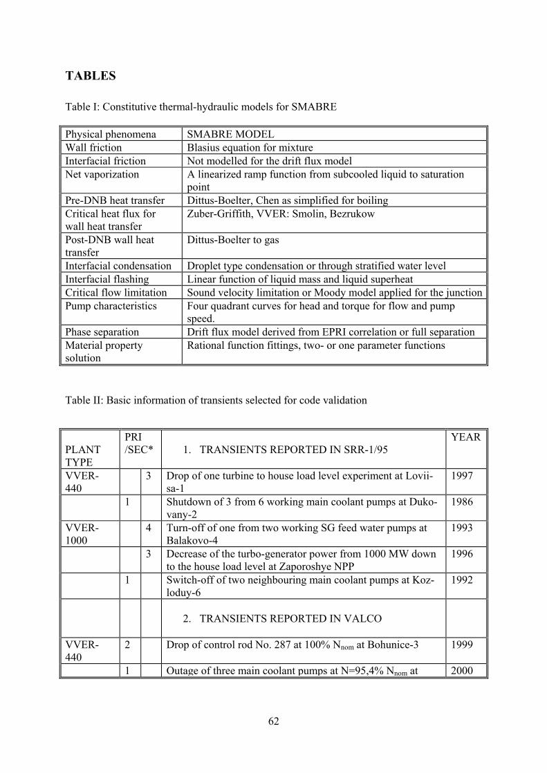
TABLES Table I: Constitutive thermal-hydraulic models for SMABRE Physical phenomena SMABRE MODEL Wall friction Blasius equation for mixture Interfacial friction Not modelled for the drift flux model Net vaporization A linearized ramp function from subcooled liquid to saturation

point Pre-DNB heat transfer Dittus-Boelter, Chen as simplified for boiling Critical heat flux for wall heat transfer

Zuber-Griffith, VVER: Smolin, Bezrukow

Post-DNB wall heat transfer

Dittus-Boelter to gas

Interfacial condensation Droplet type condensation or through stratified water level Interfacial flashing Linear function of liquid mass and liquid superheat Critical flow limitation Sound velocity limitation or Moody model applied for the junctionPump characteristics Four quadrant curves for head and torque for flow and pump

speed. Phase separation Drift flux model derived from EPRI correlation or full separation Material property solution

Rational function fittings, two- or one parameter functions

Table II: Basic information of transients selected for code validation

PLANT TYPE

PRI

/SEC*

1. TRANSIENTS REPORTED IN SRR-1/95

YEAR

VVER-440

3 Drop of one turbine to house load level experiment at Lovii-sa-1

1997

1 Shutdown of 3 from 6 working main coolant pumps at Duko-vany-2

1986

VVER-1000

4 Turn-off of one from two working SG feed water pumps at Balakovo-4

1993

3 Decrease of the turbo-generator power from 1000 MW down to the house load level at Zaporoshye NPP

1996

1 Switch-off of two neighbouring main coolant pumps at Koz-loduy-6

1992

2. TRANSIENTS REPORTED IN VALCO

VVER-440

2 Drop of control rod No. 287 at 100% Nnom at Bohunice-3 1999

1 Outage of three main coolant pumps at N=95,4% Nnom at 2000

62

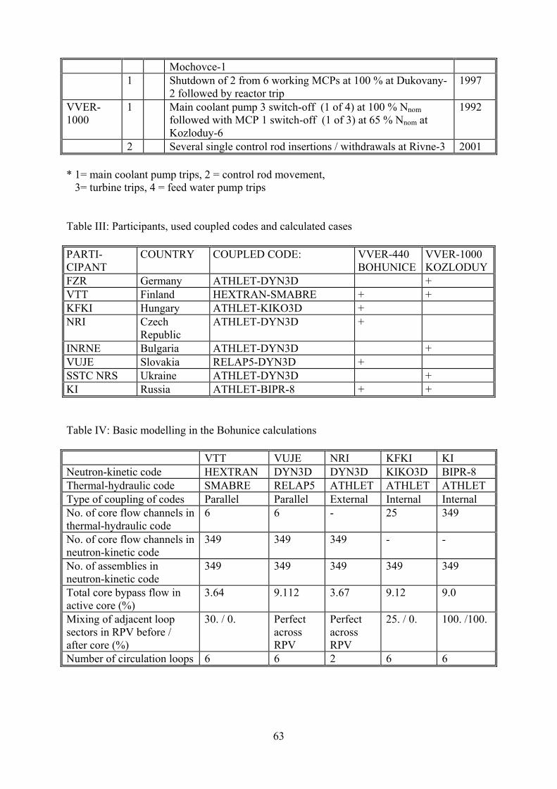
Mochovce-1 1 Shutdown of 2 from 6 working MCPs at 100 % at Dukovany-

2 followed by reactor trip 1997

VVER-1000

1 Main coolant pump 3 switch-off (1 of 4) at 100 % Nnom followed with MCP 1 switch-off (1 of 3) at 65 % Nnom at Kozloduy-6

1992

2 Several single control rod insertions / withdrawals at Rivne-3 2001 * 1= main coolant pump trips, 2 = control rod movement, 3= turbine trips, 4 = feed water pump trips Table III: Participants, used coupled codes and calculated cases PARTI-CIPANT

COUNTRY COUPLED CODE: VVER-440 BOHUNICE

VVER-1000 KOZLODUY

FZR Germany ATHLET-DYN3D + VTT Finland HEXTRAN-SMABRE + + KFKI Hungary ATHLET-KIKO3D + NRI Czech

Republic ATHLET-DYN3D +

INRNE Bulgaria ATHLET-DYN3D + VUJE Slovakia RELAP5-DYN3D + SSTC NRS Ukraine ATHLET-DYN3D + KI Russia ATHLET-BIPR-8 + + Table IV: Basic modelling in the Bohunice calculations VTT VUJE NRI KFKI KI Neutron-kinetic code HEXTRAN DYN3D DYN3D KIKO3D BIPR-8 Thermal-hydraulic code SMABRE RELAP5 ATHLET ATHLET ATHLET Type of coupling of codes Parallel Parallel External Internal Internal No. of core flow channels in thermal-hydraulic code

6 6 - 25 349

No. of core flow channels in neutron-kinetic code

349 349 349 - -

No. of assemblies in neutron-kinetic code

349 349 349 349 349

Total core bypass flow in active core (%)

3.64 9.112 3.67 9.12 9.0

Mixing of adjacent loop sectors in RPV before / after core (%)

30. / 0. Perfect across RPV

Perfect across RPV

25. / 0. 100. /100.

Number of circulation loops 6 6 2 6 6

63

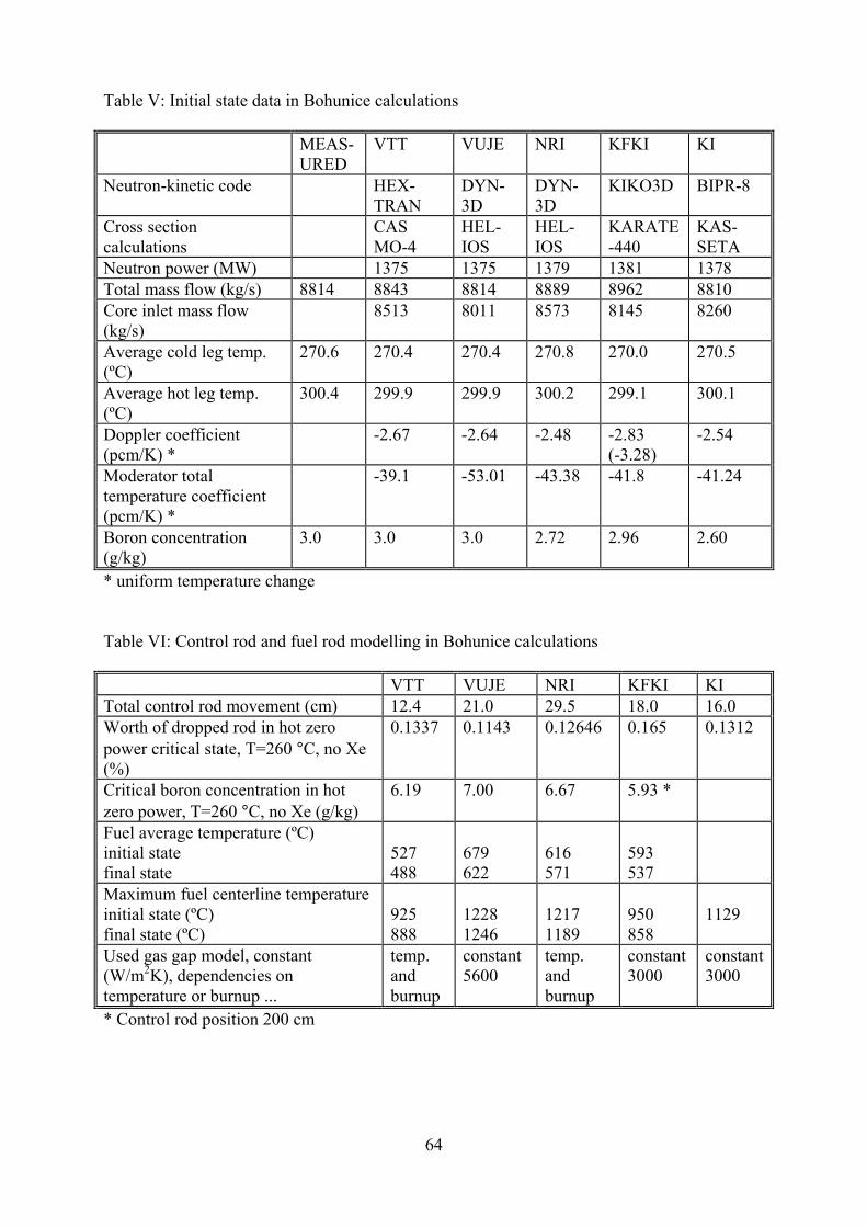
Table V: Initial state data in Bohunice calculations MEAS-

URED VTT VUJE NRI KFKI KI

Neutron-kinetic code HEX-TRAN

DYN-3D

DYN-3D

KIKO3D BIPR-8

Cross section calculations

CAS MO-4

HEL-IOS

HEL-IOS

KARATE-440

KAS-SETA

Neutron power (MW) 1375 1375 1379 1381 1378 Total mass flow (kg/s) 8814 8843 8814 8889 8962 8810 Core inlet mass flow (kg/s)

8513 8011 8573 8145 8260

Average cold leg temp. (ºC)

270.6 270.4 270.4 270.8 270.0 270.5

Average hot leg temp. (ºC)

300.4 299.9 299.9 300.2 299.1 300.1

Doppler coefficient (pcm/K) *

-2.67 -2.64 -2.48 -2.83 (-3.28)

-2.54

Moderator total temperature coefficient (pcm/K) *

-39.1 -53.01 -43.38 -41.8 -41.24

Boron concentration (g/kg)

3.0 3.0 3.0 2.72 2.96 2.60

* uniform temperature change

Table VI: Control rod and fuel rod modelling in Bohunice calculations VTT VUJE NRI KFKI KI Total control rod movement (cm) 12.4 21.0 29.5 18.0 16.0 Worth of dropped rod in hot zero power critical state, T=260 °C, no Xe (%)

0.1337 0.1143 0.12646 0.165 0.1312

Critical boron concentration in hot zero power, T=260 °C, no Xe (g/kg)

6.19 7.00 6.67 5.93 *

Fuel average temperature (ºC) initial state final state

527 488

679 622

616 571

593 537

Maximum fuel centerline temperature initial state (ºC) final state (ºC)

925 888

1228 1246

1217 1189

950 858

1129

Used gas gap model, constant (W/m2K), dependencies on temperature or burnup ...

temp. and burnup

constant 5600

temp. and burnup

constant 3000

constant3000

* Control rod position 200 cm

64

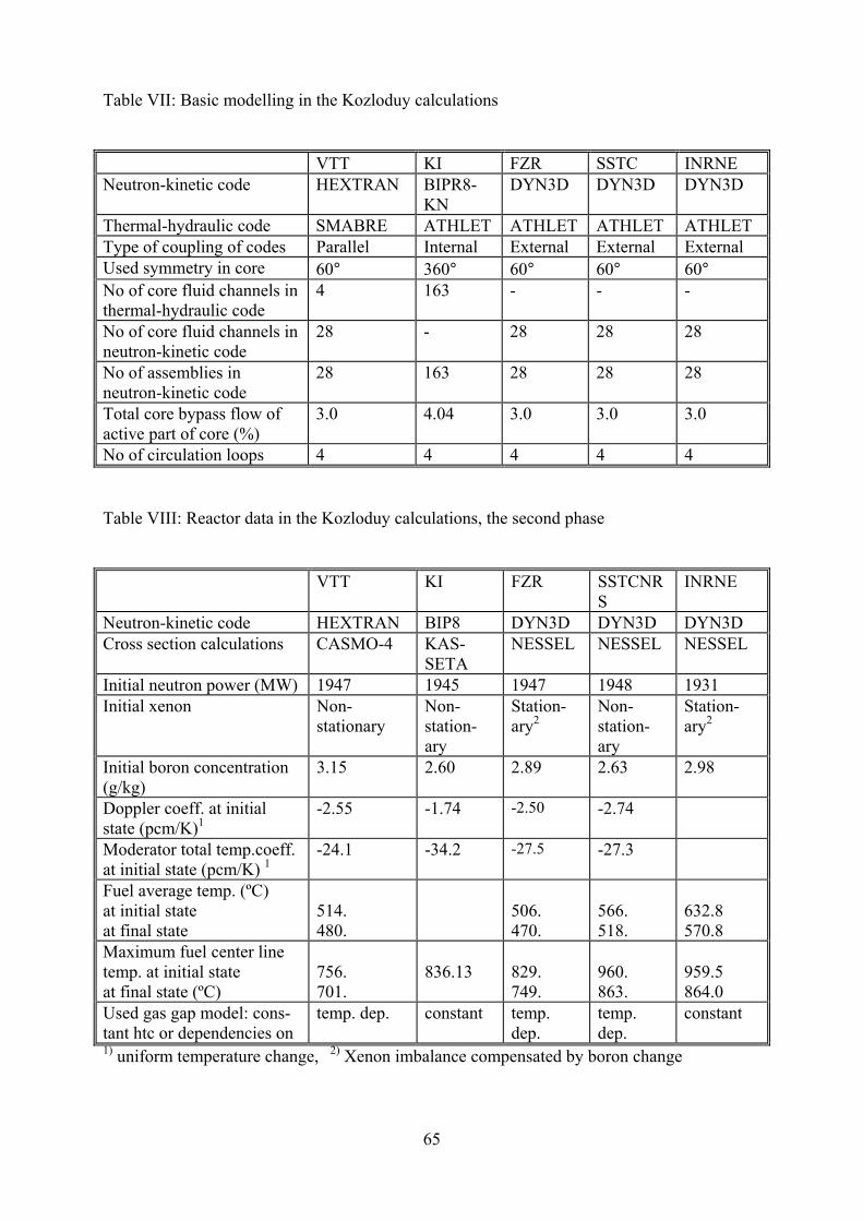
Table VII: Basic modelling in the Kozloduy calculations

VTT KI FZR SSTC INRNE Neutron-kinetic code HEXTRAN BIPR8-

KN DYN3D DYN3D DYN3D

Thermal-hydraulic code SMABRE ATHLET ATHLET ATHLET ATHLET Type of coupling of codes Parallel Internal External External External Used symmetry in core 60° 360° 60° 60° 60° No of core fluid channels in thermal-hydraulic code

4 163 - - -

No of core fluid channels in neutron-kinetic code

28 - 28 28 28

No of assemblies in neutron-kinetic code

28 163 28 28 28

Total core bypass flow of active part of core (%)

3.0 4.04 3.0 3.0 3.0

No of circulation loops 4 4 4 4 4

Table VIII: Reactor data in the Kozloduy calculations, the second phase

VTT KI FZR SSTCNRS

INRNE

Neutron-kinetic code HEXTRAN BIP8 DYN3D DYN3D DYN3D Cross section calculations CASMO-4 KAS-

SETA NESSEL NESSEL NESSEL

Initial neutron power (MW) 1947 1945 1947 1948 1931 Initial xenon Non-

stationary Non-station-ary

Station-ary2

Non-station-ary

Station-ary2

Initial boron concentration (g/kg)

3.15 2.60 2.89 2.63 2.98

Doppler coeff. at initial state (pcm/K)1

-2.55 -1.74 -2.50 -2.74

Moderator total temp.coeff. at initial state (pcm/K) 1

-24.1 -34.2 -27.5 -27.3

Fuel average temp. (ºC) at initial state at final state

514. 480.

506. 470.

566. 518.

632.8 570.8

Maximum fuel center line temp. at initial state at final state (ºC)

756. 701.

836.13

829. 749.

960. 863.

959.5 864.0

Used gas gap model: cons-tant htc or dependencies on

temp. dep. constant temp. dep.

temp. dep.

constant

1) uniform temperature change, 2) Xenon imbalance compensated by boron change

65

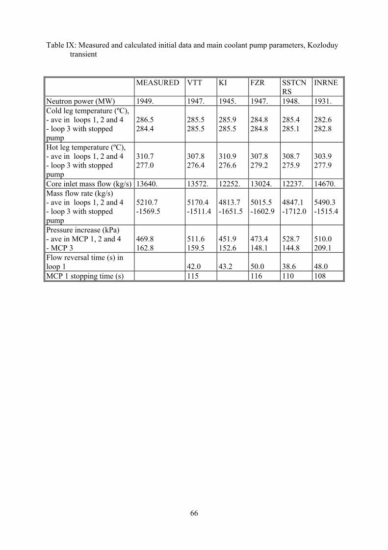
Table IX: Measured and calculated initial data and main coolant pump parameters, Kozloduy transient

MEASURED VTT KI FZR SSTCNRS

INRNE

Neutron power (MW) 1949. 1947. 1945. 1947. 1948. 1931. Cold leg temperature (ºC), - ave in loops 1, 2 and 4 - loop 3 with stopped pump

286.5 284.4

285.5 285.5

285.9 285.5

284.8 284.8

285.4 285.1

282.6 282.8

Hot leg temperature (ºC), - ave in loops 1, 2 and 4 - loop 3 with stopped pump

310.7 277.0

307.8 276.4

310.9 276.6

307.8 279.2

308.7 275.9

303.9 277.9

Core inlet mass flow (kg/s) 13640. 13572. 12252. 13024. 12237. 14670. Mass flow rate (kg/s) - ave in loops 1, 2 and 4 - loop 3 with stopped pump

5210.7 -1569.5

5170.4 -1511.4

4813.7 -1651.5

5015.5 -1602.9

4847.1 -1712.0

5490.3 -1515.4

Pressure increase (kPa) - ave in MCP 1, 2 and 4 - MCP 3

469.8 162.8

511.6 159.5

451.9 152.6

473.4 148.1

528.7 144.8

510.0 209.1

Flow reversal time (s) in loop 1

42.0

43.2

50.0

38.6

48.0

MCP 1 stopping time (s) 115 116 110 108

66

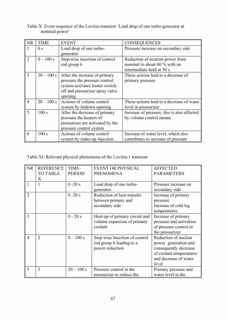
Table X: Event sequence of the Loviisa transient ‘Load drop of one turbo-generator at nominal power’

NR TIME EVENT CONSEQUENCES 1 0 s Load drop of one turbo-

generator Pressure increase on secondary side

2 0 – 100 s Step-wise insertion of control rod group 6

Reduction of neutron power from nominal to about 60 % with an intermediate hold at 50 s

3 20 – 100 s After the increase of primary pressure the pressure control system activates heater switch-off and pressurizer spray valve opening

These actions lead to a decrease of primary pressure

4 20 – 100 s Actions of volume control system by letdown opening

These actions lead to a decrease of water level in pressurizer

5 100 s After the decrease of primary pressure the heaters of pressurizer are activated by the pressure control system

Increase of pressure, this is also affected by volume control means

6 100 s Actions of volume control system by make-up injection

Increase of water level, which also contributes to increase of pressure

Table XI: Relevant physical phenomena of the Loviisa-1 transient NR REFERENCE

TO TABLE X

TIME-PERIOD

EVENT OR PHYSICAL PHENOMENA

AFFECTED PARAMETERS

1 1 0 -20 s Load drop of one turbo-generator

Pressure increase on secondary side

2 0 -20 s Reduction of heat transfer between primary and secondary side

Increase of primary pressure Increase of cold leg temperatures

3 0 - 20 s Heat-up of primary circuit and volume expansion of primary coolant

Increase of primary pressure and activation of pressure control in the pressurizer

4 2 0 – 100 s Step-wise Insertion of control rod group 6 leading to a power reduction

Reduction of nuclear power generation and consequently decrease of coolant temperatures and decrease of water level

5 3 20 – 100 s Pressure control in the pressurizer to reduce the

Primary pressure and water level in the

67

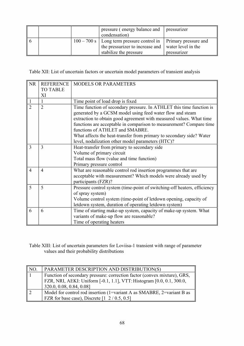
pressure ( energy balance and condensation)

pressurizer

6 100 – 700 s Long term pressure control in the pressurizer to increase and stabilize the pressure

Primary pressure and water level in the pressurizer

Table XII: List of uncertain factors or uncertain model parameters of transient analysis NR REFERENCE

TO TABLE XI

MODELS OR PARAMETERS

1 1 Time point of load drop is fixed 2 2 Time function of secondary pressure. In ATHLET this time function is

generated by a GCSM model using feed water flow and steam extraction to obtain good agreement with measured values. What time functions are acceptable in comparison to measurement? Compare time functions of ATHLET and SMABRE. What affects the heat-transfer from primary to secondary side? Water level, nodalization other model parameters (HTC)?

3 3 Heat-transfer from primary to secondary side Volume of primary circuit Total mass flow (value and time function) Primary pressure control

4 4 What are reasonable control rod insertion programmes that are acceptable with measurement? Which models were already used by participants (FZR)?

5 5 Pressure control system (time-point of switching-off heaters, efficiency of spray system) Volume control system (time-point of letdown opening, capacity of letdown system, duration of operating letdown system)

6 6 Time of starting make-up system, capacity of make-up system. What variants of make-up flow are reasonable? Time of operating heaters

Table XIII: List of uncertain parameters for Loviisa-1 transient with range of parameter

values and their probability distributions NO. PARAMETER DESCRIPTION AND DISTRIBUTION(S) 1 Function of secondary pressure: correction factor (convex mixture), GRS,

FZR, NRI, AEKI: Uniform [-0.1, 1.1], VTT: Histogram [0.0, 0.1, 300.0, 320.0, 0.08, 0.84, 0.08]

2 Model for control rod insertion (1=variant A as SMABRE, 2=variant B as FZR for base case), Discrete [1 2 / 0.5, 0.5]

68

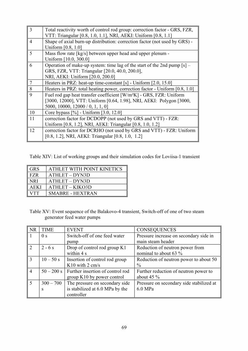
3 Total reactivity worth of control rod group: correction factor - GRS, FZR, VTT: Triangular [0.8, 1.0, 1.1], NRI, AEKI: Uniform [0.8, 1.1]

4 Shape of axial burn-up distribution: correction factor (not used by GRS) - Uniform [0.8, 1.0]

5 Mass flow rate [kg/s] between upper head and upper plenum - Uniform [10.0, 300.0]

6 Operation of make-up system: time lag of the start of the 2nd pump [s] – GRS, FZR, VTT: Triangular [20.0, 40.0, 200.0], NRI, AEKI: Uniform [20.0, 200.0]

7 Heaters in PRZ: heat-up time-constant [s] - Uniform [2.0, 15.0] 8 Heaters in PRZ: total heating power, correction factor - Uniform [0.8, 1.0] 9 Fuel rod gap heat transfer coefficient [W/m²K] - GRS, FZR: Uniform

[3000, 12000], VTT: Uniform [0.64, 1.98], NRI, AEKI: Polygon [3000, 5000, 10000, 12000 / 0, 1, 1, 0]

10 Core bypass [%] - Uniform [3.0, 12.0] 11 correction factor for DCDOPP (not used by GRS and VTT) - FZR:

Uniform [0.8, 1.2], NRI, AEKI: Triangular [0.8, 1.0, 1.2] 12 correction factor for DCRHO (not used by GRS and VTT) - FZR: Uniform

[0.8, 1.2], NRI, AEKI: Triangular [0.8, 1.0, 1.2]

Table XIV: List of working groups and their simulation codes for Loviisa-1 transient GRS ATHLET WITH POINT KINETICS FZR ATHLET – DYN3D NRI ATHLET – DYN3D AEKI ATHLET – KIKO3D VTT SMABRE - HEXTRAN Table XV: Event sequence of the Balakovo-4 transient, Switch-off of one of two steam

generator feed water pumps NR TIME EVENT CONSEQUENCES 1 0 s Switch-off of one feed water

pump Pressure increase on secondary side in main steam header

2 2 - 6 s Drop of control rod group K1 within 4 s

Reduction of neutron power from nominal to about 63 %

3 10 – 50 s Insertion of control rod group K10 with 2 cm/s

Reduction of neutron power to about 50 %

4 50 – 200 s Further insertion of control rod group K10 by power control

Further reduction of neutron power to about 45 %

5 300 – 700 s

The pressure on secondary side is stabilized at 6.0 MPa by the controller

Pressure on secondary side stabilized at 6.0 MPa

69

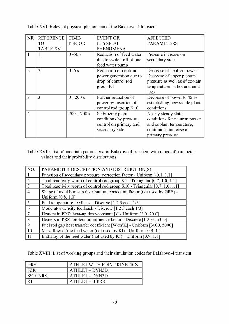
Table XVI: Relevant physical phenomena of the Balakovo-4 transient NR REFERENCE

TO TABLE XV

TIME-PERIOD

EVENT OR PHYSICAL PHENOMENA

AFFECTED PARAMETERS

1 1 0 -50 s Reduction of feed water due to switch-off of one feed water pump

Pressure increase on secondary side

2 2 0 -6 s Reduction of neutron power generation due to drop of control rod group K1

Decrease of neutron power Decrease of upper plenum pressure as well as of coolant temperatures in hot and cold legs

3 3 0 - 200 s Further reduction of power by insertion of control rod group K10

Decrease of power to 45 % establishing new stable plant conditions

4 200 – 700 s Stabilizing plant conditions by pressure control on primary and secondary side

Nearly steady state conditions for neutron power and coolant temperature, continuous increase of primary pressure

Table XVII: List of uncertain parameters for Balakovo-4 transient with range of parameter

values and their probability distributions NO. PARAMETER DESCRIPTION AND DISTRIBUTION(S) 1 Function of secondary pressure: correction factor - Uniform [-0.1, 1.1] 2 Total reactivity worth of control rod group K1 - Triangular [0.7, 1.0, 1.1] 3 Total reactivity worth of control rod group K10 - Triangular [0.7, 1.0, 1.1] 4 Shape of axial burn-up distribution: correction factor (not used by GRS) -

Uniform [0.8, 1.0] 5 Fuel temperature feedback - Discrete [1 2 3 each 1/3] 6 Moderator density feedback - Discrete [1 2 3 each 1/3] 7 Heaters in PRZ: heat-up time-constant [s] - Uniform [2.0, 20.0] 8 Heaters in PRZ: protection influence factor - Discrete [1 2 each 0.5] 9 Fuel rod gap heat transfer coefficient [W/m²K] - Uniform [3000, 5000] 10 Mass flow of the feed water (not used by KI) - Uniform [0.9, 1.1] 11 Enthalpy of the feed water (not used by KI) - Uniform [0.9, 1.1] Table XVIII: List of working groups and their simulation codes for Balakovo-4 transient GRS ATHLET WITH POINT KINETICS FZR ATHLET – DYN3D SSTCNRS ATHLET – DYN3D KI ATHLET – BIPR8

70

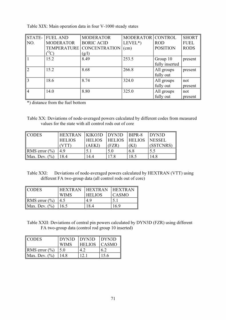
Table XIX: Main operation data in four V-1000 steady states STATE- NO.

FUEL AND MODERATOR TEMPERATURE (OC)

MODERATOR BORIC ACID CONCENTRATION (g/l)

MODERATOR LEVEL*) (cm)

CONTROL ROD POSITION

SHORT FUEL RODS

1

15.2

8.49

253.5

Group 10 fully inserted

present

2 15.2 8.68 266.8 All groups fully out

present

3 18.6 8.74 324.0 All groups fully out

not present

4 14.0 8.80 325.0 All groups fully out

not present

*) distance from the fuel bottom Table XX: Deviations of node-averaged powers calculated by different codes from measured

values for the state with all control rods out of core CODES HEXTRAN

HELIOS (VTT)

KIKO3D HELIOS (AEKI)

DYN3D HELIOS (FZR)

BIPR-8 HELIOS (KI)

DYN3D NESSEL (SSTCNRS)

RMS error (%) 4.9 5.1 5.0 6.8 5.5 Max. Dev. (%) 18.4 14.4 17.8 18.5 14.8 Table XXI: Deviations of node-averaged powers calculated by HEXTRAN (VTT) using

different FA two-group data (all control rods out of core) CODES HEXTRAN

WIMS HEXTRAN HELIOS

HEXTRAN CASMO

RMS error (%) 4.5 4.9 5.1 Max. Dev. (%) 16.5 18.4 16.9 Table XXII: Deviations of central pin powers calculated by DYN3D (FZR) using different

FA two-group data (control rod group 10 inserted) CODES DYN3D

WIMS DYN3D HELIOS CASMO

RMS error (%) 5.0 4.2 6.2 Max. Dev. (%) 14.8 12.1 15.6

DYN3D

71

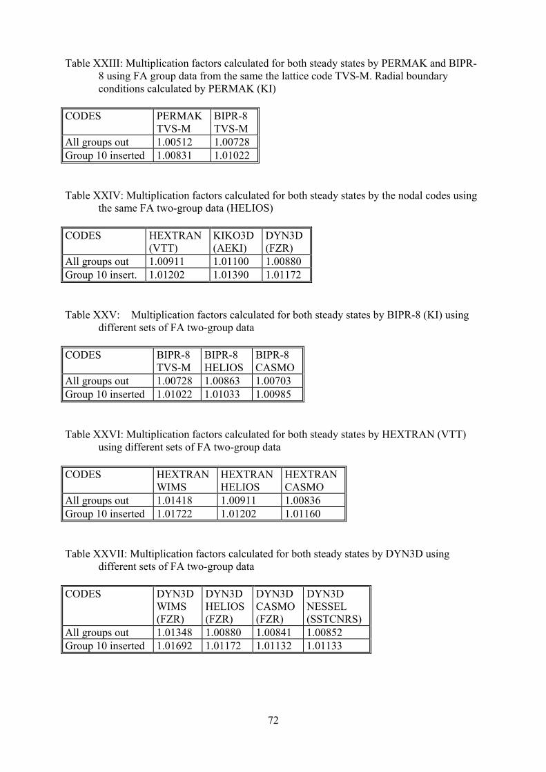
Table XXIII: Multiplication factors calculated for both steady states by PERMAK and BIPR-8 using FA group data from the same the lattice code TVS-M. Radial boundary conditions calculated by PERMAK (KI)

CODES PERMAK

TVS-M BIPR-8 TVS-M

All groups out 1.00512 1.00728 Group 10 inserted 1.00831 1.01022 Table XXIV: Multiplication factors calculated for both steady states by the nodal codes using

the same FA two-group data (HELIOS) CODES HEXTRAN

(VTT) KIKO3D (AEKI)

DYN3D (FZR)

All groups out 1.00911 1.01100 1.00880 Group 10 insert. 1.01202 1.01390 1.01172 Table XXV: Multiplication factors calculated for both steady states by BIPR-8 (KI) using

different sets of FA two-group data CODES BIPR-8

TVS-M BIPR-8 HELIOS

BIPR-8 CASMO

All groups out 1.00728 1.00863 1.00703 Group 10 inserted 1.01022 1.01033 1.00985 Table XXVI: Multiplication factors calculated for both steady states by HEXTRAN (VTT)

using different sets of FA two-group data CODES HEXTRAN

WIMS HEXTRAN HELIOS

HEXTRAN CASMO

All groups out 1.01418 1.00911 1.00836 Group 10 inserted 1.01722 1.01202 1.01160 Table XXVII: Multiplication factors calculated for both steady states by DYN3D using

different sets of FA two-group data CODES DYN3D

WIMS (FZR)

DYN3D HELIOS (FZR)

DYN3D CASMO (FZR)

DYN3D NESSEL (SSTCNRS)

All groups out 1.01348 1.00880 1.00841 1.00852 Group 10 inserted 1.01692 1.01172 1.01132 1.01133

72

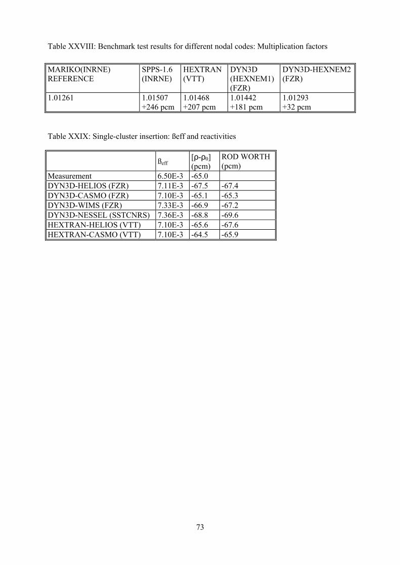
Table XXVIII: Benchmark test results for different nodal codes: Multiplication factors MARIKO(INRNE) REFERENCE

SPPS-1.6 (INRNE)

HEXTRAN (VTT)

DYN3D (HEXNEM1) (FZR)

DYN3D-HEXNEM2(FZR)

1.01261 1.01507 +246 pcm

1.01468 +207 pcm

1.01442 +181 pcm

1.01293 +32 pcm

Table XXIX: Single-cluster insertion: ßeff and reactivities ßeff

[ρ-ρ0] (pcm)

ROD WORTH (pcm)

Measurement 6.50E-3 -65.0 DYN3D-HELIOS (FZR) 7.11E-3 -67.5 -67.4 DYN3D-CASMO (FZR) 7.10E-3 -65.1 -65.3 DYN3D-WIMS (FZR) 7.33E-3 -66.9 -67.2 DYN3D-NESSEL (SSTCNRS) 7.36E-3 -68.8 -69.6 HEXTRAN-HELIOS (VTT) 7.10E-3 -65.6 -67.6 HEXTRAN-CASMO (VTT) 7.10E-3 -64.5 -65.9

73

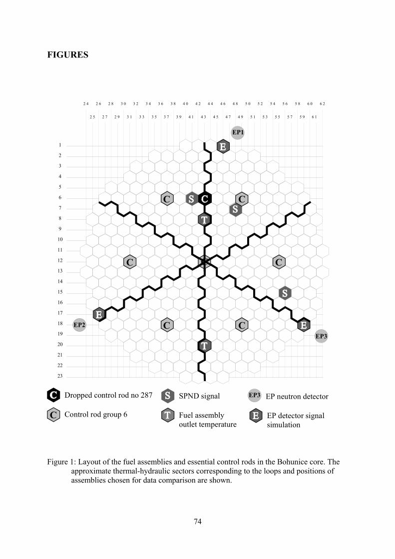
FIGURES

2 4 2 6 2 8 3 0 3 2 3 4 3 6 3 8 4 0 4 2 4 4 4 6 4 8 5 0 5 2 5 4 5 6 5 8 6 0 6 2

2 5 2 7 2 9 3 1 3 3 3 5 3 7 3 9 4 1 4 3 4 5 4 7 4 9 5 1 5 3 5 5 5 7 5 9 6 1

1

2

3

4

5

6

7

8

9

10

11

12

13

14

15

16

17

18

19

20

21

22

23

EP3

EP2

EP1

SPND signal

Fuel assembly outlet temperature

EP detector signal simulation

Dropped control rod no 287

Control rod group 6

EP neutron detector

C C

C

CC

C

C

C

EP3

Figure 1: Layout of the fuel assemblies and essential control rods in the Bohunice core. The

approximate thermal-hydraulic sectors corresponding to the loops and positions of assemblies chosen for data comparison are shown.

74

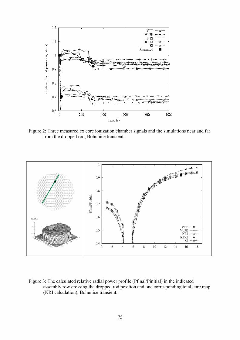
Figure 2: Three measured ex core ionization chamber signals and the simulations near and far

from the dropped rod, Bohunice transient.

Figure 3: The calculated relative radial power profile (Pfinal/Pinitial) in the indicated

assembly row crossing the dropped rod position and one corresponding total core map (NRI calculation), Bohunice transient.

75

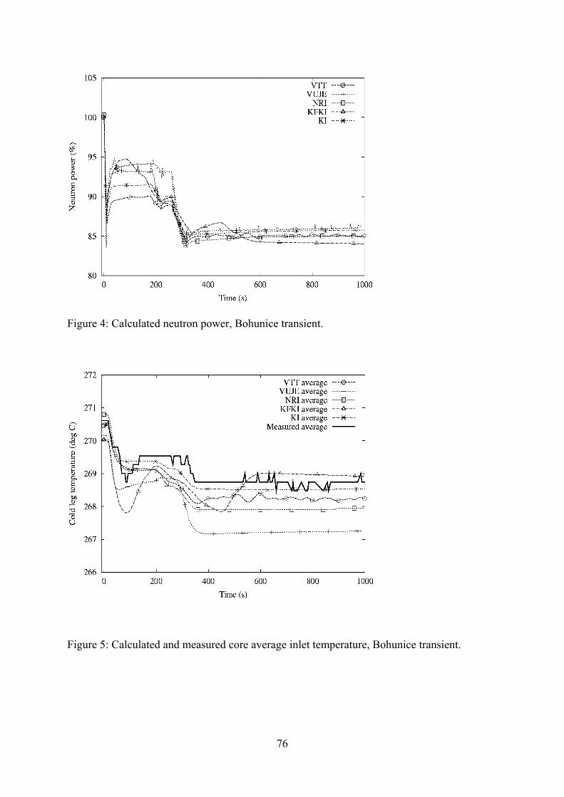
Figure 4: Calculated neutron power, Bohunice transient.

Figure 5: Calculated and measured core average inlet temperature, Bohunice transient.

76

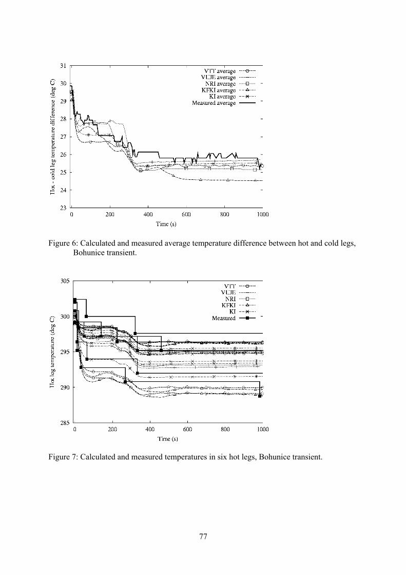
Figure 6: Calculated and measured average temperature difference between hot and cold legs, Bohunice transient.

Figure 7: Calculated and measured temperatures in six hot legs, Bohunice transient.

77

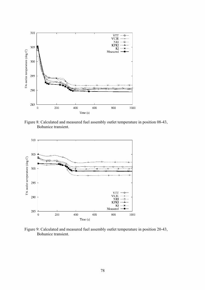
Figure 8: Calculated and measured fuel assembly outlet temperature in position 08-43, Bohunice transient.

Figure 9: Calculated and measured fuel assembly outlet temperature in position 20-43, Bohunice transient.

78

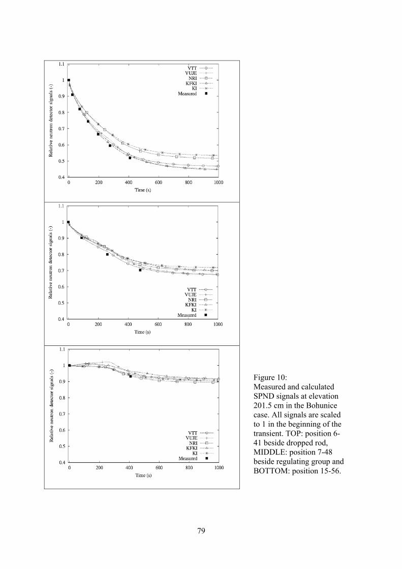
Figure 10: Measured and calculated SPND signals at elevation 201.5 cm in the Bohunice case. All signals are scaled to 1 in the beginning of the transient. TOP: position 6-41 beside dropped rod, MIDDLE: position 7-48 beside regulating group and BOTTOM: position 15-56.

79

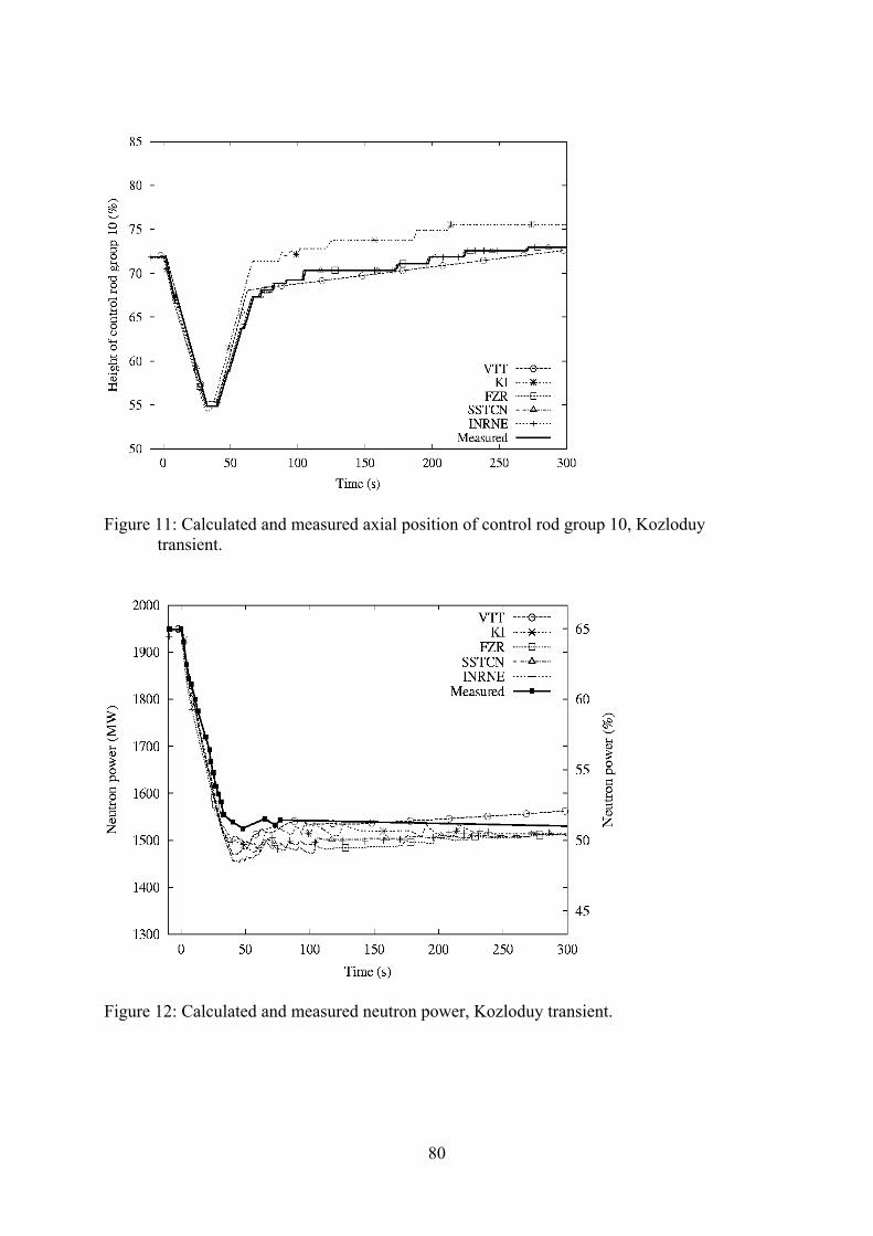
Figure 11: Calculated and measured axial position of control rod group 10, Kozloduy transient.

Figure 12: Calculated and measured neutron power, Kozloduy transient.

80

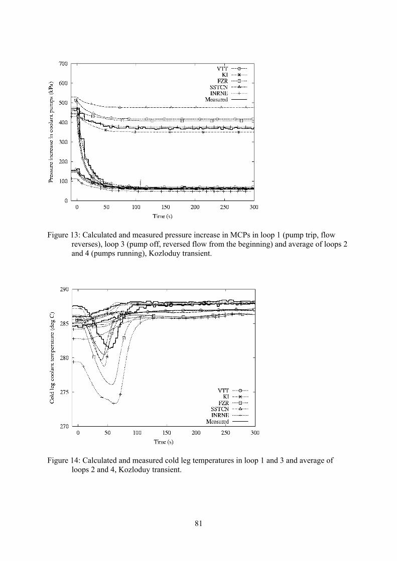
Figure 13: Calculated and measured pressure increase in MCPs in loop 1 (pump trip, flow reverses), loop 3 (pump off, reversed flow from the beginning) and average of loops 2 and 4 (pumps running), Kozloduy transient.

Figure 14: Calculated and measured cold leg temperatures in loop 1 and 3 and average of loops 2 and 4, Kozloduy transient.

81

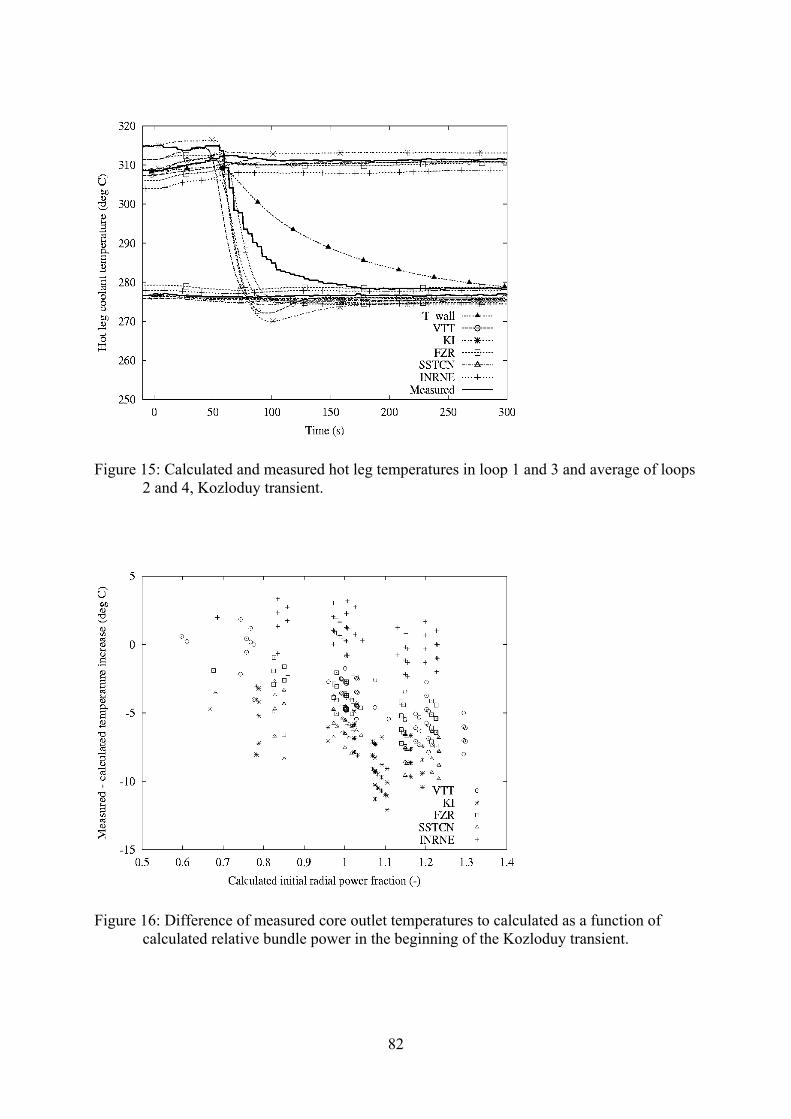
Figure 15: Calculated and measured hot leg temperatures in loop 1 and 3 and average of loops 2 and 4, Kozloduy transient.

Figure 16: Difference of measured core outlet temperatures to calculated as a function of calculated relative bundle power in the beginning of the Kozloduy transient.

82

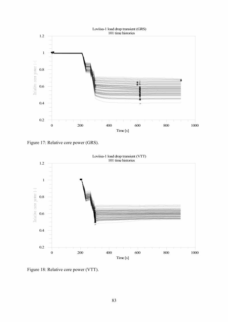
101 time histories

Loviisa-1 load drop transient (GRS)

Time [s]10008006004002000

1.2

1

0.8

0.6

0.4

0.2

1

1

2

2

3

3

4

4

5

5

6

6

7

7

8

8

9

9

10

10

11

11

12

12

13

13

14

14

15

15

16

16

17

17

18

18

19

19

20

20

21

21

22

22

23

23

24

24

25

25

26

26

27

27

28

28

29

29

30

30

31

31

32

32

33

33

34

34

35

35

36

36

37

37

38

38

39

39

40

40

41

41

42

42

43

43

44

44

45

45

46

46

47

47

48

48

49

49

50

50

51

51

52

52

53

53

54

54

55

55

56

56

57

57

58

58

59

59

60

60

61

61

62

62

63

63

64

64

65

65

66

66

67

67

68

68

69

69

70

70

71

71

72

72

73

73

74

74

75

75

76

76

77

77

78

78

79

79

80

80

81

81

82

82

83

83

84

84

85

85

86

86

87

87

88

88

89

89

90

90

91

91

92

92

93

93

94

94

95

95

96

96

97

97

98

98

99

99

100

100

101

101

Figure 17: Relative core power (GRS).

101 time histories

Loviisa-1 load drop transient (VTT)

Time [s]10008006004002000

1.2

1

0.8

0.6

0.4

0.2

1

1

2

2

3

3

4

4

5

5

6

6

7

7

8

8

9

9

10

10

11

11

12

12

13

13

14

14

15

15

16

16

17

17

18

18

19

19

20

20

21

21

22

22

23

23

24

24

25

25

26

26

27

27

28

28

29

29

30

30

31

31

32

32

33

33

34

34

35

35

36

36

37

37

38

38

39

39

40

40

41

41

42

42

43

43

44

44

45

45

46

46

47

47

48

48

49

49

50

50

51

51

52

52

53

53

54

54

55

55

56

56

57

57

58

58

59

59

60

60

61

61

62

62

63

63

64

64

65

65

66

66

67

67

68

68

69

69

70

70

71

71

72

72

73

73

74

74

75

75

76

76

77

77

78

78

79

79

80

80

81

81

82

82

83

83

84

84

85

85

86

86

87

87

88

88

89

89

90

90

91

91

92

92

93

93

94

94

95

95

96

96

97

97

98

98

99

99

100

100

101

101

Figure 18: Relative core power (VTT).

83

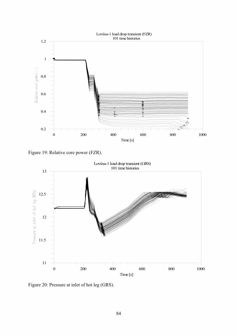
101 time histories

Loviisa-1 load drop transient (FZR)

Time [s]10008006004002000

1.2

1

0.8

0.6

0.4

0.2

1

1

2

2

3

3

4

4

5

5

6

6

7

7

8

8

9

9

10

10

11

11

12

12

13

13

14

14

15

15

16

16

17

17

18

18

19

19

20

20

21

21

22

22

23

23

24

24

25

25

26

26

27

27

28

28

29

29

30

30

31

31

32

32

33

33

34

34

35

35

36

36

37

37

38

38

39

39

40

40

41

41

42

42

43

43

44

44

45

45

46

46

47

47

48

48

49

49

50

50

51

51

52

52

53

53

54

54

55

55

56

56

57

57

58

58

59

59

60

60

61

61

62

62

63

63

64

64

65

65

66

66

67

67

68

68

69

69

70

70

71

71

72

72

73

73

74

74

75

75

76

76

77

77

78

78

79

79

80

80

81

81

82

82

83

83

84

84

85

85

86

86

87

87

88

88

89

89

90

90

91

91

92

92

93

93

94

94

95

95

96

96

97

97

98

98

99

99

100

100

101

101

Figure 19: Relative core power (FZR).

101 time histories

Loviisa-1 load drop transient (GRS)

Time [s]10008006004002000

13

12.5

12

11.5

11

1

1

2

2

3

3

4

4

5

5

6

6

7

7

8

8

9

9

10

10

11

11

12

12

13

13

14

14

15

15

16

16

17

17

18

18

19

19

20

20

21

21

22

22

23

23

24

24

25

25

26

26

27

27

28

28

29

29

30

30

31

31

32

32

33

33

34

34

35

35

36

36

37

37

38

38

39

39

40

40

41

41

42

42

43

43

44

44

45

45

46

46

47

47

48

48

49

49

50

50

51

51

52

52

53

53

54

54

55

55

56

56

57

57

58

58

59

59

60

60

61

61

62

62

63

63

64

64

65

65

66

66

67

67

68

68

69

69

70

70

71

71

72

72

73

73

74

74

75

75

76

76

77

77

78

78

79

79

80

80

81

81

82

82

83

83

84

84

85

85

86

86

87

87

88

88

89

89

90

90

91

91

92

92

93

93

94

94

95

95

96

96

97

97

98

98

99

99

100

100

101

101

Figure 20: Pressure at inlet of hot leg (GRS).

84

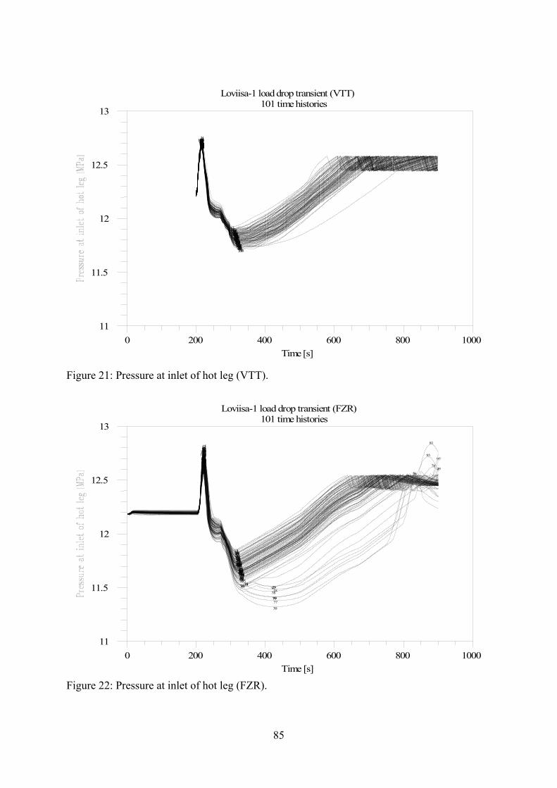
101 time histories

Loviisa-1 load drop transient (VTT)

Time [s]10008006004002000

13

12.5

12

11.5

11

1

1

2

2

3

3

4

4

5

5

6

6

7

7

8

8

9

9

10

10

11

11

12

12

13

13

14

14

15

15

16

16

17

17

18

18

19

19

20

20

21

21

22

22

23

23

24

24

25

25

26

26

27

27

28

28

29

29

30

30

31

31

32

32

33

33

34

34

35

35

36

36

37

37

38

38

39

39

40

40

41

41

42

42

43

43

44

44

45

45

46

46

47

47

48

48

49

49

50

50

51

51

52

52

53

53

54

54

55

55

56

56

57

57

58

58

59

59

60

60

61

61

62

62

63

63

64

64

65

65

66

66

67

67

68

68

69

69

70

70

71

71

72

72

73

73

74

74

75

75

76

76

77

77

78

78

79

79

80

80

81

81

82

82

83

83

84

84

85

85

86

86

87

87

88

88

89

89

90

90

91

91

92

92

93

93

94

94

95

95

96

96

97

97

98

98

99

99

100

100

101

101

Figure 21: Pressure at inlet of hot leg (VTT).

Figure 22: Pressure at inlet of hot leg (FZR).

101 time histories

Loviisa-1 load drop transient (FZR)

Time [s]10008006004002000

13

12.5

12

11.5

11

1

1

2

2

3

3

4

4

5

5

6

6

7

7

8

8

9

9

10

10

11

11

12

12

13

13

14

14

15

15

16

16

17

17

18

18

19

19

20

20

21

21

22

22

23

23

24

24

25

25

26

26

27

27

28

28

29

29

30

30

31

31

32

32

33

33

34

34

35

35

36

36

37

37

38

38

39

39

40

40

41

41

42

42

43

43

44

44

45

45

46

46

47

47

48

48

49

49

50

50

51

51

52

52

53

53

54

54

55

55

56

56

57

57

58

58

59

59

60

60

61

61

62

62

63

63

64

64

65

65

66

66

67

67

68

68

69

69

70

70

71

71

72

72

73

73

74

74

75

75

76

76

77

77

78

78

79

79

80

80

81

81

82

82

83

83

84

84

85

85

86

86

87

87

88

88

89

89

90

90

91

91

92

92

93

93

94

94

95

95

96

96

97

97

98

98

99

99

100

100

101

101

85

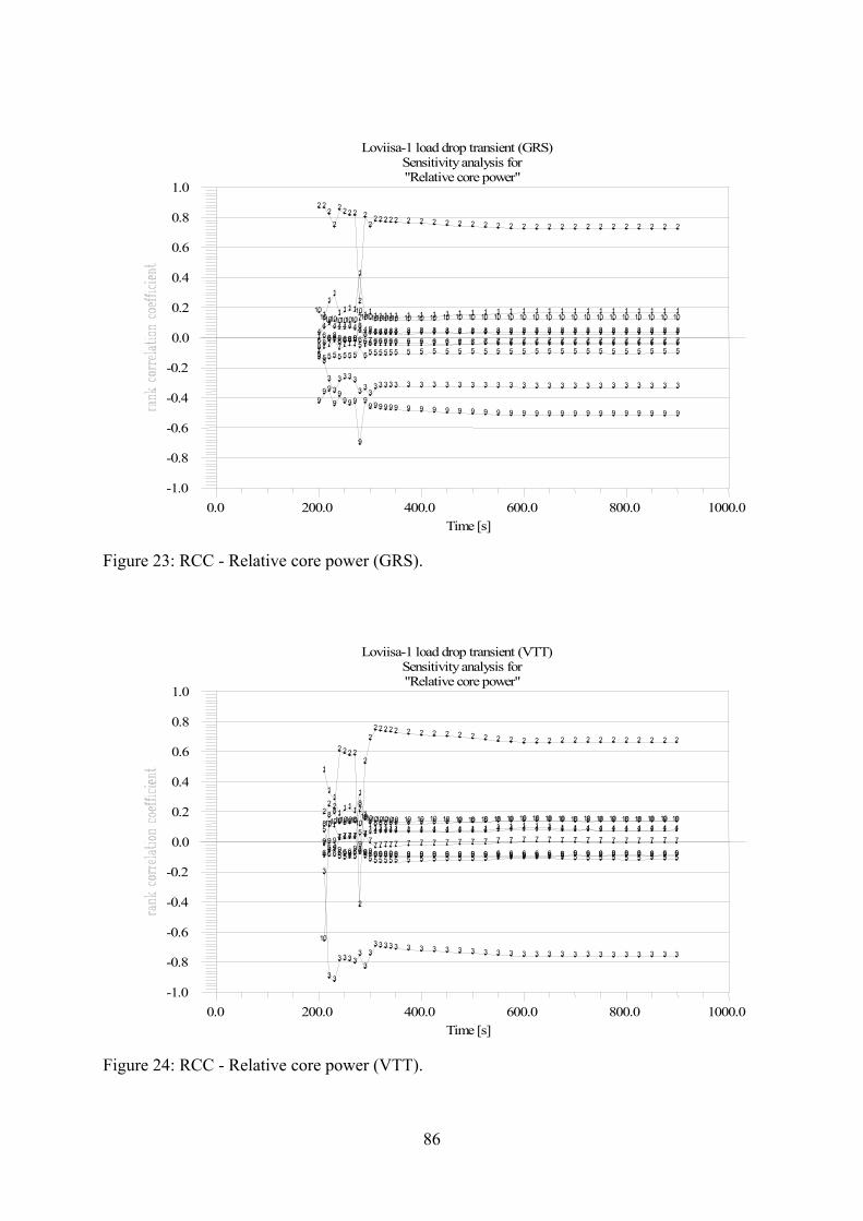
"Relative core power"Sensitivity analysis for

Loviisa-1 load drop transient (GRS)

Time [s]1000.0800.0600.0400.0200.00.0

1.0

0.8

0.6

0.4

0.2

0.0

-0.2

-0.4

-0.6

-0.8

-1.0

1

1

1 1

1 1 1 1

1

1 1 1 1 1 1 1 1 1 1 1 1 1 1 1 1 1 1 1 1 1 1 1 1 1 1 1 1 1

2 2 2

2

2 2 2 2

2

2 2

2 2 2 2 2 2 2 2 2 2 2 2 2 2 2 2 2 2 2 2 2 2 2 2 2 2 2

3 3

3 3

3 3 3 3 3 3 3

3 3 3 3 3 3 3 3 3 3 3 3 3 3 3 3 3 3 3 3 3 3 3 3 3 3 3

4 4 4 4 4 4 4 4 4 4 4 4 4 4 4 4 4 4 4 4 4 4 4 4 4 4 4 4 4 4 4 4 4 4 4 4 4 4

5 5 5 5 5 5 5 5 5

5 5 5 5 5 5 5 5 5 5 5 5 5 5 5 5 5 5 5 5 5 5 5 5 5 5 5 5 5 6

6 6 6 6 6 6 6 6 6 6 6 6 6 6 6 6 6 6 6 6 6 6 6 6 6 6 6 6 6 6 6 6 6 6 6 6 6 7 7

7 7 7 7 7 7

7

7 7 7 7 7 7 7 7 7 7 7 7 7 7 7 7 7 7 7 7 7 7 7 7 7 7 7 7 7 8 8

8 8 8 8 8 8 8

8 8 8 8 8 8 8 8 8 8 8 8 8 8 8 8 8 8 8 8 8 8 8 8 8 8 8 8 8

9 9 9

9 9

9 9 9

9

9 9 9 9 9 9 9 9 9 9 9 9 9 9 9 9 9 9 9 9 9 9 9 9 9 9 9 9 9

10 10 10 10 10 10 10 10

10 10 10 10 10 10 10 10 10 10 10 10 10 10 10 10 10 10 10 10 10 10 10 10 10 10 10 10 10 10

Figure 23: RCC - Relative core power (GRS).

"Relative core power"Sensitivity analysis for

Loviisa-1 load drop transient (VTT)

Time [s]1000.0800.0600.0400.0200.00.0

1.0

0.8

0.6

0.4

0.2

0.0

-0.2

-0.4

-0.6

-0.8

-1.0

1

1 1

1 1 1 1

1

1 1 1 1 1 1 1 1 1 1 1 1 1 1 1 1 1 1 1 1 1 1 1 1 1 1 1 1 1

2 2 2

2 2 2 2

2

2

2 2 2 2 2 2 2 2 2 2 2 2 2 2 2 2 2 2 2 2 2 2 2 2 2 2 2 2

3

3 3

3 3 3 3 3

3

3 3 3 3 3 3 3 3 3 3 3 3 3 3 3 3 3 3 3 3 3 3 3 3 3 3 3 3

4 4 4

4 4 4 4

4

4 4 4 4 4 4 4 4 4 4 4 4 4 4 4 4 4 4 4 4 4 4 4 4 4 4 4 4 4 5

5 5 5 5 5 5

5

5 5 5 5 5 5 5 5 5 5 5 5 5 5 5 5 5 5 5 5 5 5 5 5 5 5 5 5 5 6 6 6 6 6 6 6 6 6 6 6 6 6 6 6 6 6 6 6 6 6 6 6 6 6 6 6 6 6 6 6 6 6 6 6 6 6 7

7 7 7 7 7 7

7

7 7 7 7 7 7 7 7 7 7 7 7 7 7 7 7 7 7 7 7 7 7 7 7 7 7 7 7 7

8 8 8

8 8 8 8

8

8 8 8 8 8 8 8 8 8 8 8 8 8 8 8 8 8 8 8 8 8 8 8 8 8 8 8 8 8

9 9 9 9 9 9 9

9 9 9 9 9 9 9 9 9 9 9 9 9 9 9 9 9 9 9 9 9 9 9 9 9 9 9 9 9 9

10

10 10 10 10 10 10 10 10 10 10 10 10 10 10 10 10 10 10 10 10 10 10 10 10 10 10 10 10 10 10 10 10 10 10 10 10

Figure 24: RCC - Relative core power (VTT).

86

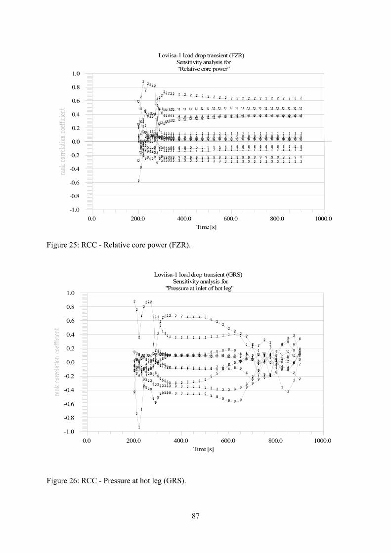
"Relative core power"Sensitivity analysis for

Loviisa-1 load drop transient (FZR)

Time [s]1000.0800.0600.0400.0200.00.0

1.0

0.8

0.6

0.4

0.2

0.0

-0.2

-0.4

-0.6

-0.8

-1.0

1

1

1 1

1 1 1 1

1

1 1 1 1 1 1 1 1 1 1 1 1 1 1 1 1 1 1 1 1 1 1 1 1 1 1 1 1 1 2

2

2

2

2 2 2 2

2

2 2 2 2 2 2 2 2 2 2 2 2 2 2 2 2 2 2 2 2 2 2 2 2 2 2 2 2 2

3

3 3 3 3 3 3 3 3

3 3 3 3 3 3 3 3 3 3 3 3 3 3 3 3 3 3 3 3 3 3 3 3 3 3 3 3 3

4

4

4

4

4 4 4 4

4

4 4

4 4 4 4 4 4 4 4 4 4 4 4 4 4 4 4 4 4 4 4 4 4 4 4 4 4 4

5

5 5 5 5 5 5 5

5

5 5 5 5 5 5 5 5 5 5 5 5 5 5 5 5 5 5 5 5 5 5 5 5 5 5 5 5 5 6 6 6

6 6 6 6 6 6

6 6 6 6 6 6 6 6 6 6 6 6 6 6 6 6 6 6 6 6 6 6 6 6 6 6 6 6 6 7

7 7 7 7 7 7 7

7

7 7 7 7 7 7 7 7 7 7 7 7 7 7 7 7 7 7 7 7 7 7 7 7 7 7 7 7 7

8 8 8

8 8 8 8 8

8 8 8 8 8 8 8 8 8 8 8 8 8 8 8 8 8 8 8 8 8 8 8 8 8 8 8 8 8 8

9

9

9 9 9 9 9 9

9 9 9 9 9 9 9 9 9 9 9 9 9 9 9 9 9 9 9 9 9 9 9 9 9 9 9 9 9 9

10 10

10 10 10 10 10 10 10 10 10 10 10 10 10 10 10 10 10 10 10 10 10 10 10 10 10 10 10 10 10 10 10 10 10 10 10 10

11

11

11

11 11 11 11 11

11 11 11 11 11 11 11 11 11 11 11 11 11 11 11 11 11 11 11 11 11 11 11 11 11 11 11 11 11 11

12

12 12

12 12 12 12 12

12 12 12 12 12 12 12 12 12 12 12 12 12 12 12 12 12 12 12 12 12 12 12 12 12 12 12 12 12 12

Figure 25: RCC - Relative core power (FZR).

"Pressure at inlet of hot leg"

Sensitivity analysis forLoviisa-1 load drop transient (GRS)

Time [s]1000.0800.0600.0400.0200.00.0

1.0

0.8

0.6

0.4

0.2

0.0

-0.2

-0.4

-0.6

-0.8

-1.0

1

1

1

1

1

1 1

1

1

1 1

1 1 1

1 1 1 1 1 1 1 1 1 1 1 1 1 1

1 1 1

1 1

1

1 1

1

1

2

2

2

2

2 2 2 2

2

2

2

2 2 2 2 2 2 2 2 2 2 2 2 2

2 2

2 2

2

2 2 2

2

2

2 2 2

2

3 3

3

3

3 3 3 3 3 3 3 3 3 3 3 3 3 3 3 3 3 3 3 3 3 3 3 3

3

3

3

3 3

3

3

3 3

3

4

4 4

4 4

4 4 4 4

4 4 4 4 4 4 4 4 4 4 4 4 4 4 4 4 4 4 4

4 4

4 4

4

4 4 4

4

4

5 5

5 5

5 5 5 5 5 5 5

5 5 5 5 5 5 5 5 5 5 5 5

5 5

5 5 5

5 5

5

5 5

5

5 5

5

5

6 6 6 6 6 6 6 6 6 6 6 6 6 6 6 6 6 6 6 6 6 6 6 6 6 6 6 6

6

6

6

6

6 6

6 6

6 6

7 7

7 7 7 7 7 7 7

7 7 7 7 7 7 7 7 7 7 7 7 7 7 7 7 7

7 7 7 7

7

7

7

7 7 7 7 7 8

8 8 8 8

8 8 8 8 8 8 8 8 8

8 8 8 8 8 8 8 8 8 8 8 8 8 8 8

8

8 8

8 8

8 8

8

8

9

9 9

9

9 9 9 9

9 9

9 9 9 9 9 9 9 9 9 9 9 9 9 9 9 9 9 9

9 9

9 9 9

9

9 9

9

9

10

10 10 10 10 10 10 10 10 10 10 10 10 10 10 10 10 10 10 10 10 10 10 10 10 10 10

10 10 10 10 10

10 10

10 10

10 10

Figure 26: RCC - Pressure at hot leg (GRS).

87

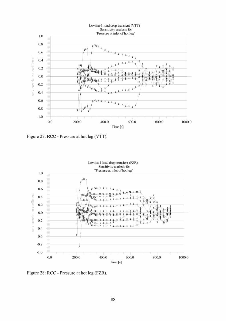
"Pressure at inlet of hot leg"

Sensitivity analysis forLoviisa-1 load drop transient (VTT)

Time [s]1000.0800.0600.0400.0200.00.0

1.0

0.8

0.6

0.4

0.2

0.0

-0.2

-0.4

-0.6

-0.8

-1.0

1

1

1 1 1

1

1 1

1 1

1

1 1 1 1 1 1 1 1 1 1 1 1 1 1 1 1 1

1 1 1 1 1

1

1 1

1

1

2

2

2 2

2 2 2

2

2 2

2

2 2 2 2 2 2

2 2 2 2 2 2 2 2 2 2

2

2

2

2 2

2 2

2

2 2

2

3 3

3

3 3 3

3 3

3 3

3

3 3 3 3 3 3 3 3 3 3 3 3 3 3 3 3

3

3 3

3 3

3

3 3

3

3 3

4

4

4 4

4 4

4 4 4

4 4 4 4 4 4 4 4 4 4 4 4 4 4 4 4 4 4

4 4 4 4 4 4

4

4

4

4 4

5 5

5 5 5

5 5 5 5 5

5 5 5 5 5 5 5 5

5 5

5 5

5 5 5 5 5

5

5

5 5

5 5

5

5

5 5

5 6 6

6 6 6 6 6

6 6 6 6 6 6 6 6

6

6 6 6 6 6 6 6 6 6 6

6 6

6 6 6 6

6

6 6

6

6 6

7 7

7 7

7 7 7 7

7 7

7 7 7 7 7 7 7 7 7 7 7 7 7 7 7 7 7 7

7

7

7

7

7

7 7

7

7 7

8

8 8

8 8 8 8 8

8 8 8 8 8 8 8 8 8 8

8 8 8 8 8 8 8 8

8

8

8 8

8 8

8 8

8

8

8

8

9

9

9 9 9 9

9 9 9

9 9 9 9 9 9 9 9 9 9 9 9 9 9 9 9 9 9 9

9

9

9

9

9

9

9

9

9

9

10

10

10 10 10 10 10 10

10 10 10 10 10 10 10 10 10 10 10 10 10 10 10 10 10 10 10

10

10

10

10 10 10

10

10 10

10 10

Figure 27: RCC - Pressure at hot leg (VTT).

"Pressure at inlet of hot leg"

Sensitivity analysis forLoviisa-1 load drop transient (FZR)

Time [s]1000.0800.0600.0400.0200.00.0

1.0

0.8

0.6

0.4

0.2

0.0

-0.2

-0.4

-0.6

-0.8

-1.0

1

1 1

1

1

1 1 1

1

1 1

1 1 1 1 1 1 1 1 1 1 1 1 1 1 1 1 1 1 1

1

1

1

1

1 1 1

1 2 2

2

2 2 2 2 2

2

2

2

2 2 2 2 2 2 2 2 2 2 2 2 2

2 2 2 2 2

2 2

2 2

2

2 2 2 2 3 3

3 3 3 3 3 3

3 3 3

3 3 3 3 3 3 3 3 3 3 3 3 3 3 3 3 3 3 3 3 3

3 3 3

3 3 3

4

4 4

4

4 4 4 4

4 4

4 4 4 4 4 4 4 4 4 4 4 4 4 4 4 4 4 4

4

4

4 4

4 4

4 4

4

4

5 5 5 5

5 5 5

5 5 5

5 5 5 5 5 5 5 5 5 5 5 5

5 5

5 5

5 5 5

5

5 5

5 5 5

5 5 5

6 6 6

6 6 6 6 6

6 6 6 6 6 6 6 6 6 6 6 6 6 6 6 6 6 6 6 6 6

6

6

6 6 6

6

6

6

6 7

7 7 7 7 7 7

7 7

7 7 7 7 7 7 7 7 7 7 7 7 7 7 7 7 7 7 7 7

7 7 7 7

7 7 7

7

7

8 8 8 8 8 8 8 8

8

8 8 8 8 8 8 8 8 8 8 8 8 8 8 8 8 8 8 8

8

8 8

8 8

8

8

8

8

8

9

9

9

9

9 9 9 9 9 9 9

9 9 9 9 9 9 9 9 9 9 9 9 9 9 9 9 9 9 9

9 9 9

9

9

9 9 9

10

10 10 10 10 10 10 10 10

10 10 10 10 10 10 10 10 10 10 10 10 10 10 10 10 10 10 10 10

10

10

10

10 10

10

10 10 10

11

11 11

11 11 11 11 11 11

11 11 11 11 11 11 11 11 11 11 11 11 11 11 11 11 11 11 11 11

11 11

11

11

11

11 11

11

11

12

12 12 12

12 12

12 12

12

12 12

12 12 12 12 12 12 12 12 12 12 12 12 12 12 12 12 12 12

12 12

12

12

12

12

12 12

12

Figure 28: RCC - Pressure at hot leg (FZR).

88

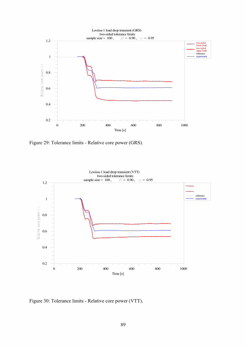
= 0.95 = 0.90 , sample size = 100 ,

two-sided tolerance limits Loviisa-1 load drop transient (GRS)

Time [s]10008006004002000

1.2

1

0.8

0.6

0.4

0.2

referenceexperiment

upper limittwo-sidedlower limittwo-sided

upper limittwo-sidedlower limittwo-sided

Figure 29: Tolerance limits - Relative core power (GRS).

= 0.95 = 0.90 , sample size = 100 ,

two-sided tolerance limits Loviisa-1 load drop transient (VTT)

Time [s]10008006004002000

1.2

1

0.8

0.6

0.4

0.2

referenceexperiment

Figure 30: Tolerance limits - Relative core power (VTT).

89

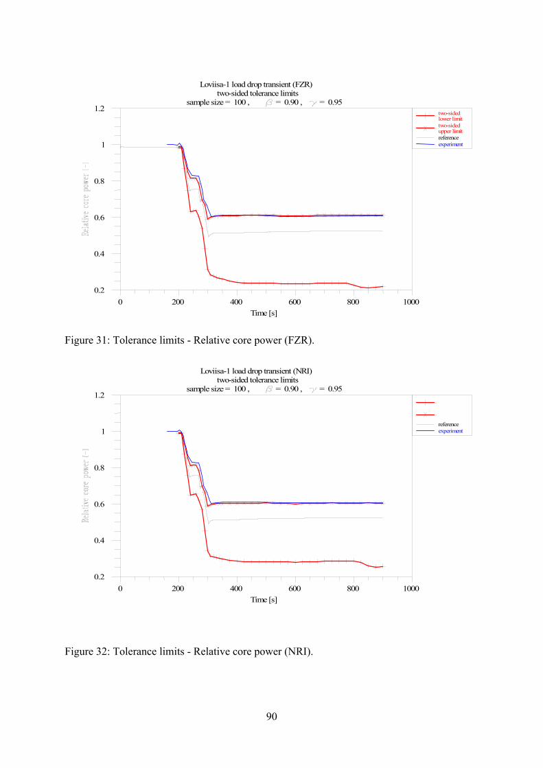
= 0.95 = 0.90 , sample size = 100 ,

two-sided tolerance limits Loviisa-1 load drop transient (FZR)

Time [s]10008006004002000

1.2

1

0.8

0.6

0.4

0.2

referenceexperiment

upper limittwo-sidedlower limittwo-sided

upper limittwo-sidedlower limittwo-sided

Figure 31: Tolerance limits - Relative core power (FZR).

= 0.95 = 0.90 , sample size = 100 ,

two-sided tolerance limits Loviisa-1 load drop transient (NRI)

Time [s]10008006004002000

1.2

1

0.8

0.6

0.4

0.2

referenceexperiment

Figure 32: Tolerance limits - Relative core power (NRI).

90

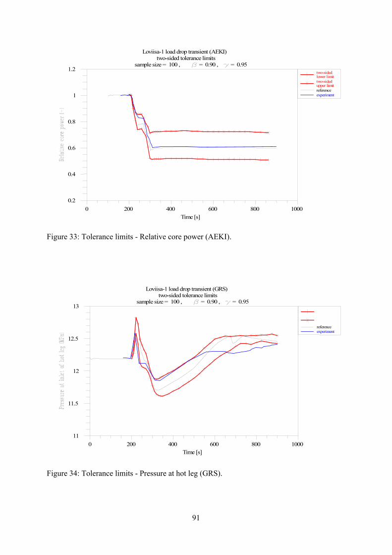
= 0.95 = 0.90 , sample size = 100 ,

two-sided tolerance limits Loviisa-1 load drop transient (AEKI)

Time [s]10008006004002000

1.2

1

0.8

0.6

0.4

0.2

referenceexperiment

upper limittwo-sidedlower limittwo-sided

upper limittwo-sidedlower limittwo-sided

Figure 33: Tolerance limits - Relative core power (AEKI).

= 0.95 = 0.90 , sample size = 100 ,

two-sided tolerance limits Loviisa-1 load drop transient (GRS)

Time [s]10008006004002000

13

12.5

12

11.5

11

referenceexperiment

Figure 34: Tolerance limits - Pressure at hot leg (GRS).

91

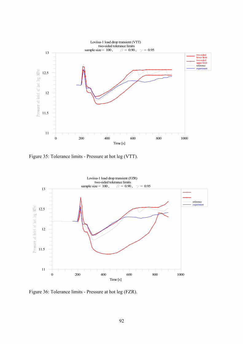
= 0.95 = 0.90 , sample size = 100 ,

two-sided tolerance limits Loviisa-1 load drop transient (VTT)

Time [s]10008006004002000

13

12.5

12

11.5

11

referenceexperiment

upper limittwo-sidedlower limittwo-sided

upper limittwo-sidedlower limittwo-sided

Figure 35: Tolerance limits - Pressure at hot leg (VTT).

= 0.95 = 0.90 , sample size = 100 ,

two-sided tolerance limits Loviisa-1 load drop transient (FZR)

Time [s]10008006004002000

13

12.5

12

11.5

11

referenceexperiment

Figure 36: Tolerance limits - Pressure at hot leg (FZR).

92

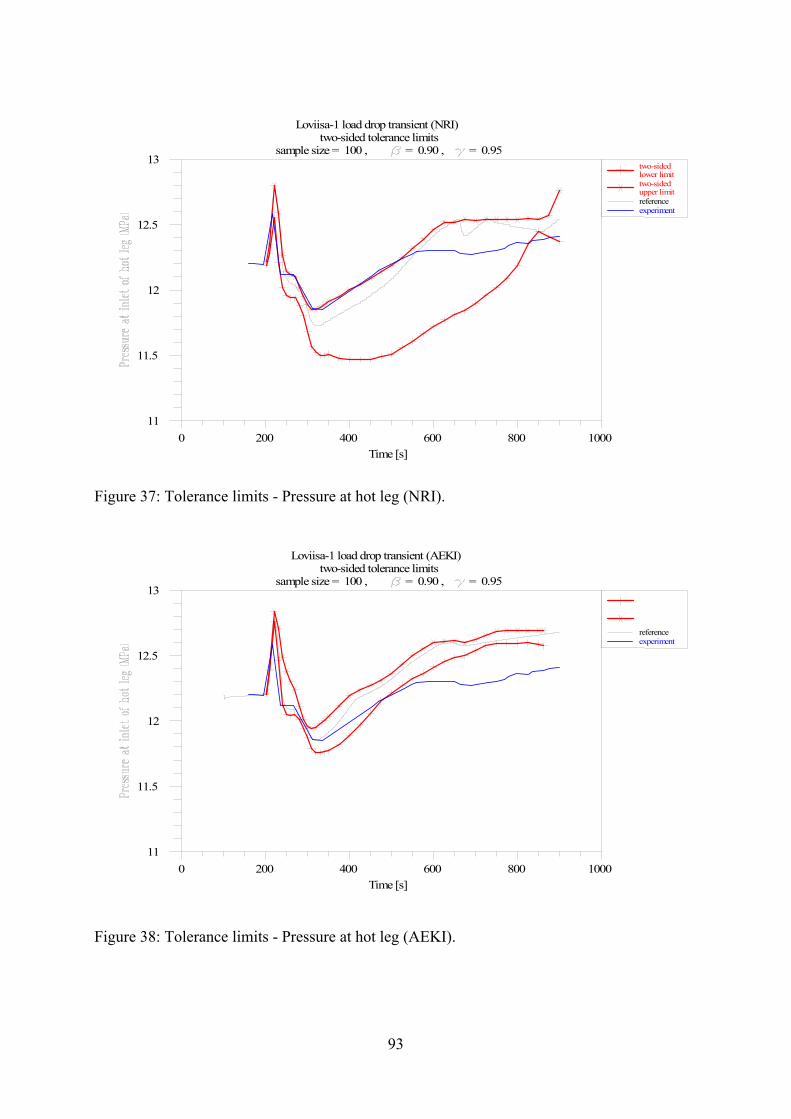
= 0.95 = 0.90 , sample size = 100 ,

two-sided tolerance limits Loviisa-1 load drop transient (NRI)

Time [s]10008006004002000

13

12.5

12

11.5

11

referenceexperiment

upper limittwo-sidedlower limittwo-sided

upper limittwo-sidedlower limittwo-sided

Figure 37: Tolerance limits - Pressure at hot leg (NRI).

= 0.95 = 0.90 , sample size = 100 ,

two-sided tolerance limits Loviisa-1 load drop transient (AEKI)

Time [s]10008006004002000

13

12.5

12

11.5

11

referenceexperiment

Figure 38: Tolerance limits - Pressure at hot leg (AEKI).

93

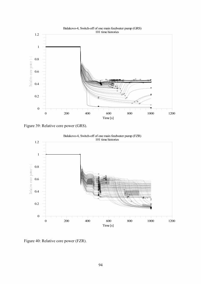
101 time histories

Balakovo-4, Switch-off of one main feedwater pump (GRS)

Time [s]120010008006004002000

1.2

1

0.8

0.6

0.4

0.2

0

1

1

2

2

3

3

4

4

5

5

6 6

7

7

8

8

9

9

10

10

11

11

12

12

13

13

14

14

15 15

16

16

17

17

18

18

19

19

20

20

21

21

22

22

23

23

24

24

25

25

26

26

27

27

28

28

29 29

30 30 31

31

32

32

33

33

34

34

35

35

36

36

37

37

38

38

39

39

40

40

41

41

42

42

43

43

44

44

45

45

46

46

47

47

48

48

49

49

50

50

51

51

52

52

53

53

54

54

55

55

56

56

57

57

58

58

59

59

60

60

61 61

62

62

63

63

64

64

65 65

66

66 67

67

68

68

69

69

70

70

71

71

72

72

73

73

74

74

75

75

76

76

77

77

78

78

79

79

80

80

81

81

82

82

83

83

84

84

85

85

86

86

87

87

88

88

89

89

90 90

91

91

92

92

93

93

94

94

95

95

96

96

97

97

98

98 99

99

100

100

101

101

Figure 39: Relative core power (GRS).

101 time histories

Balakovo-4, Switch-off of one main feedwater pump (FZR)

Time [s]120010008006004002000

1.2

1

0.8

0.6

0.4

0.2

0

1

1 2

2 3

3 4

4

5

5

6

6

7

7

8

8

9

9

10

10

11

11

12

12

13

13

14

14

15

15

16

16

17

17

18

18 19

19

20

20

21

21 22

22

23

23

24

24

25

25

26

26

27

27

28

28

29

29

30

30

31 31

32

32

33

33

34

34

35

35

36

36

37

37 38

38

39

39

40

40

41

41

42 42

43

43

44

44

45

45

46

46

47

47 48

48

49

49

50

50

51

51

52

52

53

53

54

54

55

55

56

56

57

57

58

58

59

59

60

60

61

61

62

62

63

63

64

64

65

65

66

66 68

68 69

69

70

70

71

71

72

72

74

74

75

75

76

76

77

77

78

78

79

79

80

80

81

81

82

82

83

83 84

84 85

85

86

86 87

87

88

88

89

89

90

90

91

91

92

92

93

93

94

94

95

95

96

96

97

97

98

98

99

99

100

100

101101

Figure 40: Relative core power (FZR).

94

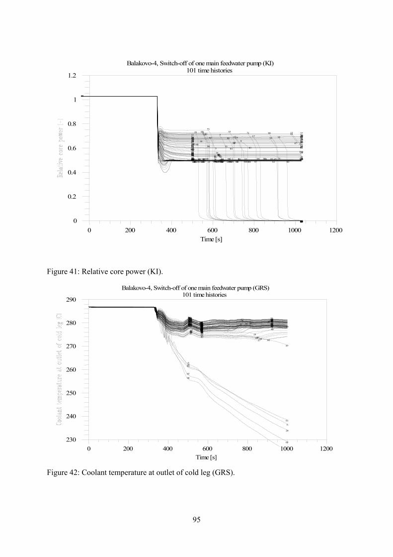
101 time histories

Balakovo-4, Switch-off of one main feedwater pump (KI)

Time [s]120010008006004002000

1.2

1

0.8

0.6

0.4

0.2

0

1 1

2 2

3 3

4 4

5

5

6

6

7 7

8 8

9

9

10 10

11

11

12 12

13 13

14 14

15 15

16 16

17

17

18 18

19

19

20 20

21 21

22

22

23

23

24 24

25 25

26 26

27 27

28 28

29 29

30 30

31 31

32 32

33 33

34 34

35 35

36 36

37 37

38 38

39

39

40 40

41 41

42 42 43

43 44

44 45

45

46 46

47 47

48 48

49 49

50 50

51

51

52 52

53

53

54 54

55 55

56 56

57 57

58 58

59 59

60 60

61 61

62 62

63 63

64 64

65 65

66 66

67

67

68 68

69

69

70 70

71

71

72 72

73

73

74 74 75

75

76 76

77 77

78 78

79 79

80 80

81

81

82 82

83 83 84

84

85 85

86

86

87 87

88 88

89 89

90 90

91 91

92

92

93 93

94 94

95

95

96 96

97 97

98 98

99

99

100100

101101

Figure 41: Relative core power (KI).

101 time histories

Balakovo-4, Switch-off of one main feedwater pump (GRS)

Time [s]120010008006004002000

290

280

270

260

250

240

230

1

1

2

2

3

3

4

4

5

5

6

6

7

7

8

8

9

9 10

10

11

11 12

12

13

13

14

14 15

15

16

16

17

17 18

18

19

19

20

20

21

21

22

22 23

23

24

24

25

25

26

26 27

27

28

28

29

29

30

30 31

31

32

32 33

33

34

34

35

35 36

36

37

37

38

38

39

39

40

40 41

41

42

42

43

43

44

44

45

45

46

46 47

47

48

48

49

49 50

50 51

51

52

52

53

53

54

54 55

55

56

56

57

57

58

58

59

59 60

60

61

61

62

62

63

63

64

64

65

65

66

66 67

67

68

68

69

69 70

70

71

71 72

72

73

73

74

74 75

75

76

76 77

77

78

78 79

79 80

80

81

81

82

82

83

83

84

84 85

85

86

86

87

87

88

88

89

89

90

91

91

92

92 93

93 94

94

95

95

96

96

97

97 98

98 99

99

100

100

101

101

Figure 42: Coolant temperature at outlet of cold leg (GRS).

95

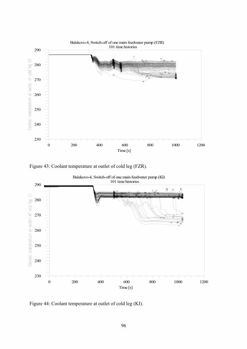
101 time histories

Balakovo-4, Switch-off of one main feedwater pump (FZR)

Time [s]120010008006004002000

290

280

270

260

250

240

230

1

1

2

2

3

3

4

4 5

5

6

6 7

7

8

8

9

9

10

10

11

11 12

12

13

13

14

14 15

15

16

16 17

17 18

18

19

19

20

20

21

21

22

22 23

23

24

24

25

25

26

26

27

27

28

28

29

29

30

30

31

31

32

32 33

33

34

34

35

35

36

36

37

37 38

38 39

39

40

40

41

41

42

42

43

43

44

44

45

45

46

46 47

47

48

48

49

49

50

50 51

51 52

52

53

53

54

54

55

55

56

56

57

57

58

58

59

59

60

60 61

61 62

62

63

63

64

64

65

65

66

66 68

68

69

69

70

70

71

71

72

72

74

74 75

75

76

76

77

77

78

78

79

79

80

80

81

81

82

82

83

83

84

84 85

85 86

86

87

87

88

88

89

89

90

90

91

91

92

92

93

93

94

94 95

95

96

96

97

97 98

98 99

99

100

100

101

101

Figure 43: Coolant temperature at outlet of cold leg (FZR).

101 time histories

Balakovo-4, Switch-off of one main feedwater pump (KI)

Time [s]120010008006004002000

290

280

270

260

250

240

230

1 1

2 2

3 3 4

4

5

5

6

6

7 7

8 8

9

9

10 10

11

11

12 12 13

13

14 14 15

15

16 16

17

17

18 18

19

19

20 20

21 21

22

22

23

23

24 24 25

25

26 26

27 27

28 28

29 29

30 30

31 31

32 32

33 33

34 34

35 35 36 36

37 37

38 38

39

39

40 40

41 41 42

42 43 43 44

44 45

45 46

46

47 47

48 48 49

49 50

50

51

51

52 52

53

53

54 54 55

55

56 56

57 57

58 58

59 59 60

60 61

61

62 62

63 63 64

64

65 65

66 66

67

67

68 68

69

69

70 70

71

71

72 72

73

73

74 74

75 75

76 76 77

77 78

78

79 79

80 80

81

81

82 82

83 83 84

84 85 85

86

86

87 87 88

88 89

89 90

90 91 91

92

92

93 93

94 94

95

95

96 96

97 97

98 98

99

99

100100101

101

Figure 44: Coolant temperature at outlet of cold leg (KI).

96

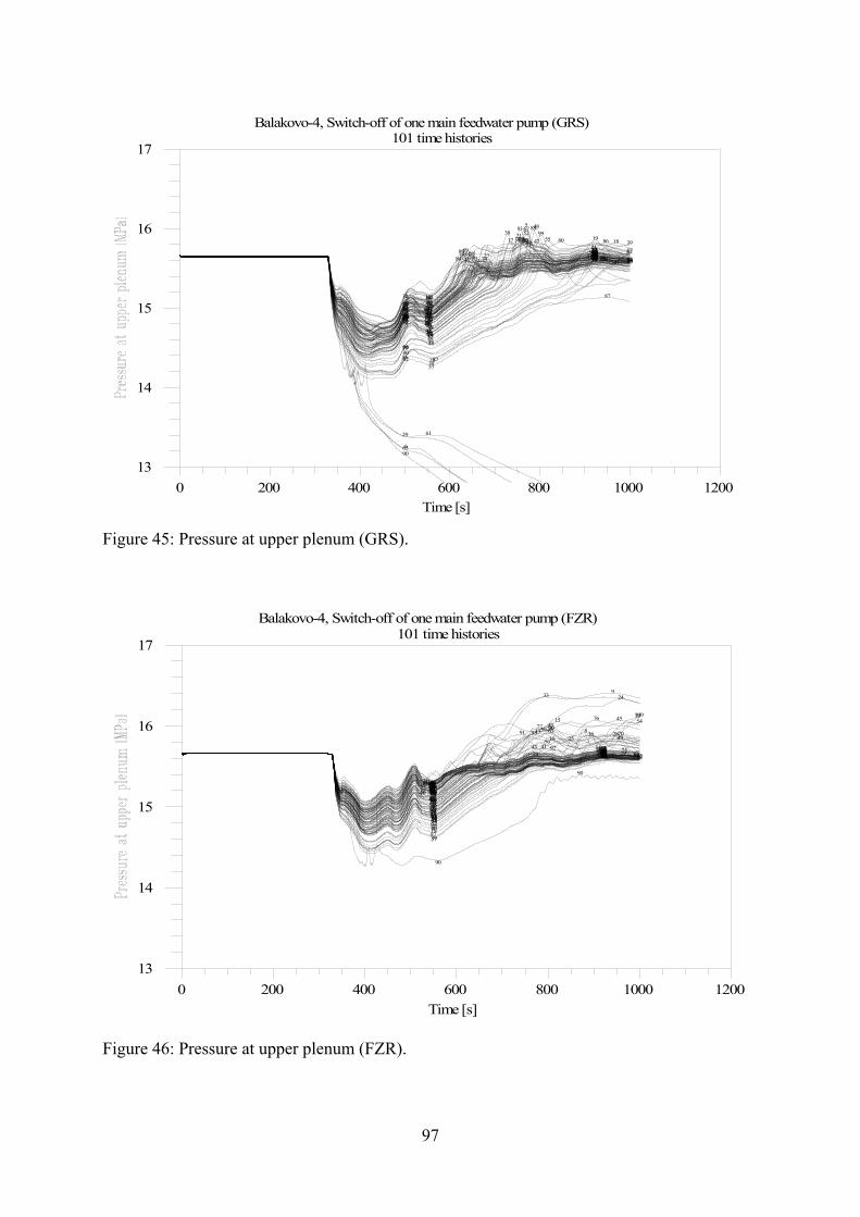
101 time histories

Balakovo-4, Switch-off of one main feedwater pump (GRS)

Time [s]120010008006004002000

17

16

15

14

13

1

1

2

2

3

3

4

4

5

5

6

7

7

8

8

9

9

10

10

11

11

12

12

13

13

14

14

15

15

16

16

17

17

18

18

19

19

20

20

21

21

22

22

23

23

24

24

25

25

26

26

27

27

28

28

29

30

30

31

31

32

32

33

33

34

34

35

35

36

36

37

37

38

38

39

39

40

40

41

41

42

42

43

43

44

44

45

45

46

46

47

47

48

48

49

49

50

50

51

51

52

52

53

53

54

54

55

55

56

56

57

57

58

58

59

59

60

60

61

62

62

63

63

64

64

65

66

66

67

67

68

68

69

69

70

70

71

71

72

72

73

73

74

74

75

75

76

76

77

77

78

78

79

79

80

80

81

81

82

82

83

83

84

84

85

85

86

86

87

87

88

88

89

89

90

91

91

92

92

93

93

94

94

95

95

96

96

97

97

98

98

99

99

100

100

101

101

Figure 45: Pressure at upper plenum (GRS).

101 time histories

Balakovo-4, Switch-off of one main feedwater pump (FZR)

Time [s]120010008006004002000

17

16

15

14

13

1

1

2

2

3

3

4

4

5

5

6

6

7

7

8

8

9

9

10

10

11

11

12

12

13

13

14

14

15

15

16

16

17

17

18

18

19

19

20

20

21

21

22

22

23

23

24

24

25

25

26

26

27

27

28

28

29

29

30

30

31

31

32

32

33

33

34

34

35

35

36

36

37

37

38

38

39

39

40

40

41

41

42

42

43

43

44

44

45

45

46

46

47

47

48

48

49

49

50

50

51

51

52

52

53

53

54

54

55

55

56

56

57

57

58

58

59

59

60

60

61

61

62

62

63

63

64

64

65

65

66

66

68

68

69

69

70

70

71

71

72

72

74

74

75

75

76

76

77

77

78

78

79

79

80

80

81

81

82

82

83

83

84

84

85

85

86

86

87

87

88

88

89

89

90

90

91

91

92

92

93

93

94

94

95

95

96

96

97

97

98

98

99

99

100

100

101

101

Figure 46: Pressure at upper plenum (FZR).

97

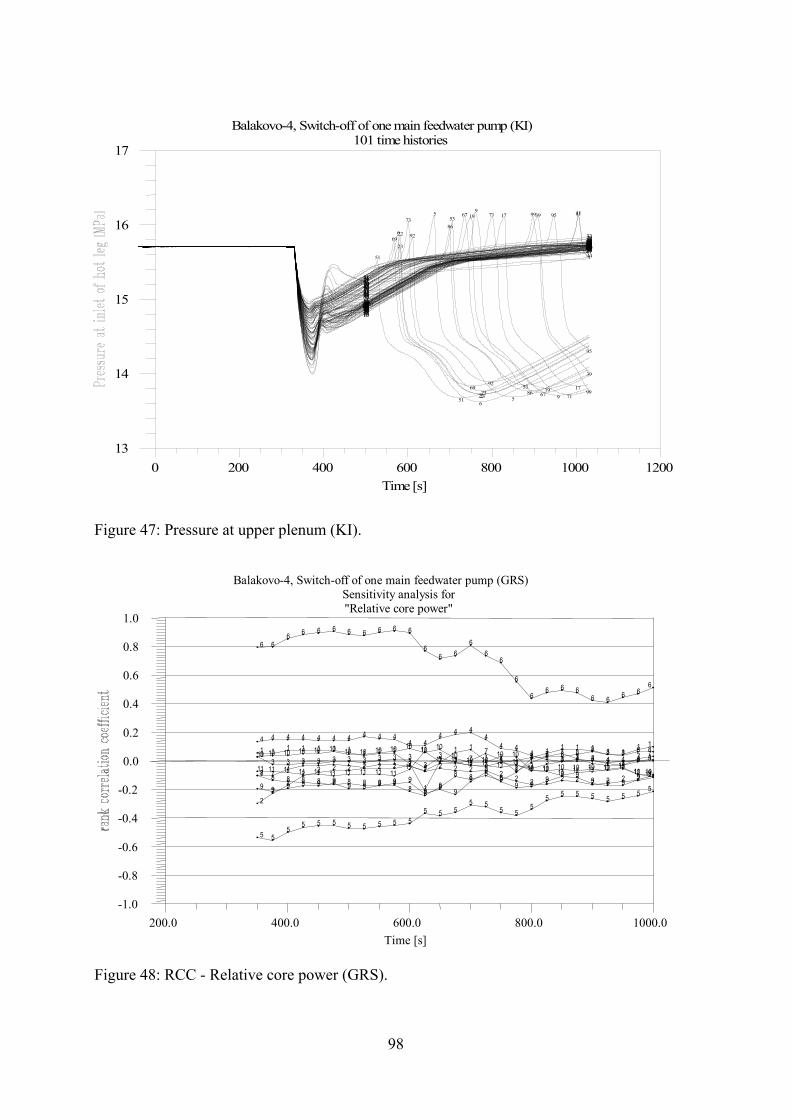
101 time histories

Balakovo-4, Switch-off of one main feedwater pump (KI)

Time [s]120010008006004002000

17

16

15

14

13

1

1

2

2

3

3

4

4

5

5

6

6

7

7

8

8

9

9

10

10

11

11

12

12

13

13

14

14

15

15

16

16

17

17

18

18

19

19

20

20

21

21

22

22

23

23

24

24

25

25

26

26

27

27

28

28

29

29

30

30

31

31

32

32

33

33

34

34

35

35

36

36

37

37

38

38

39

39

40

40

41

41

42

42

43

43

44

44

45

45

46

46

47

47

48

48

49

49

50

50

51

51

52

52

53

53

54

54

55

55

56

56

57

57

58

58

59

59

60

60

61

61

62

62

63

63

64

64

65

65

66

66

67

67

68

68

69

69

70

70

71

71

72

72

73

73

74

74

75

75

76

76

77

77

78

78

79

79

80

80

81

81

82

82

83

83

84

84

85

85

86

86

87

87

88

88

89

89

90

90

91

91

92

92

93

93

94

94

95

95

96

96

97

97

98

98

99

99

100

100

101

101

Figure 47: Pressure at upper plenum (KI).

"Relative core power"Sensitivity analysis for

Balakovo-4, Switch-off of one main feedwater pump (GRS)

Time [s]1000.0800.0600.0400.0 200.0

1.0 0.8 0.6 0.4 0.2 0.0

-0.2 -0.4 -0.6 -0.8 -1.0

1 1 1 1 1 1 1 1 1 1 1

1

1 1 1

1 1 1 1 1 1 1 1 1 1 1 1

2 2 2 2 2 2 2 2 2 2 2 2 2 2 2 2 2 2 2 2 2 2 2 2 2 2 2

3 3 3 3 3 3 3 3 3 3 3

3 3 3 3 3 3 3 3 3 3 3 3 3 3 3 3 4 4 4 4 4 4 4 4 4 4

4 4 4 4 4

4 4 4

4 4 4 4 4 4 4 4 4

5 5 5 5 5 5 5 5 5 5 5 5 5 5

5 5 5 5

5 5 5 5 5 5 5 5 5

6 6 6 6 6 6 6 6 6 6 6

6 6 6

6 6

6

6

6 6 6 6

6 6 6 6 6

7 7 7 7 7 7 7 7 7 7 7 7 7 7 7

7 7

7 7

7 7 7 7 7 7 7 7 8 8 8 8 8 8 8 8 8 8

8 8 8

8 8 8 8 8

8 8 8 8 8 8 8 8 8 9 9 9 9 9 9

9 9 9 9 9 9 9

9 9

9 9

9 9 9 9 9

9 9 9 9 9 10 10 10 10 10 10 10 10 10 10 10 10 1010 10 10

10 10

10 10 10 10 10 10 10 10 10 11 11 11 11 11 11 11 11 11 1111

1111 11 11 11 11 11

11 11 11 11 11 11 11 11 11

Figure 48: RCC - Relative core power (GRS).

98

"Relative core power"Sensitivity analysis for

Balakovo-4, Switch-off of one main feedwater pump (FZR)

Time [s]1000.0800.0600.0400.0200.0

1.0

0.8

0.6

0.4

0.2

0.0

-0.2

-0.4

-0.6

-0.8

-1.0

1 1 1 1 1 1 1 1 1 1 1 1 1 1

1 1

1 1 1 1 1 1 1 1 1 1 1

2 2

2 2 2 2 2 2 2 2

2 2

2 2 2 2 2 2 2 2 2 2 2 2 2 2 2 3 3 3 3 3 3 3 3 3 3 3 3 3 3

3 3

3 3 3 3 3 3 3 3 3 3 3 4 4

4 4 4 4 4 4 4 4 4 4

4

4 4 4 4 4 4 4 4 4 4 4 4 4 4

5 5 5 5 5 5 5 5

5 5 5 5 5 5

5 5 5

5 5 5 5 5 5 5 5 5 5

6 6 6 6 6 6 6 6 6

6 6

6 6

6

6

6 6

6 6 6 6 6 6 6 6 6 6

7 7 7 7 7 7 7 7 77 7 7 7 7

7 7 7 7 7 7 7 7 7 7 7 7 7 8 8 8 8 8 8 8 8 8 8

8 8 8 8 8

8 8 8 8 8 8 8 8 8 8 8 8

9 9 9 9 9 9 9 9 9 9 9 9 9 9 9 9

9 9 9 9 9 9 9 9 9 9 9

10 10 10 10 10 10 10 10 10 10

10 10 10 10

10 10 10 10 10 10 10 10 10 10 10 10 10

11 11 11 11 11 11 11 11 11

11 11 11 11 11 11

11 11 11 11 11 11 11 11 11 11 11

11

Figure 49: RCC - Relative core power (FZR).

Figure 50: RCC - Relative core power (KI).

"Relative core power"Sensitivity analysis for

Balakovo-4, Switch-off of one main feedwater pump (KI)

Time [s]1000.0800.0600.0400.0200.0

1.0

0.8

0.6

0.4

0.2

0.0

-0.2

-0.4

-0.6

-0.8

-1.0

1 1 1 1 1 1 1

1 1

1 1 1

1 1 1 1 1 1 1 1 1 1 1

1 1 1 1

2 2

2 2 2 2 2 2 2 2 2

2 2 2 2 2 2 2 2 2 2 2 2 2 2

2 2

3 3 3 3 3 3 3 3 3

3 3 3 3 3

3 3 3 3 3 3 3 3 3

3 3 3 3

4 4 4 4 4

4 4 4

4

4 4 4 4

4 4 4 4 4 4 4 4 4 4 4 4 4 4

5 5 5 5 5 5 5 5 5

5

5 5 5

5 5

5 5 5 5

5 5 5 5

5 5 5 5

6 6 6 6 6 6 6 6 6 6 6 6 6

6 6 6

6 6 6 6 6 6 6

6 6 6 6 7 7 7 7 7 7 7 7 7

7 7 7 7 7 7 7 7 7 7 7 7 7 7

7 7 7 7

8 8 8 8 8 8 8 8 8 8

8 8 8 8 8 8 8 8 8 8 8 8 8 8 8 8 8

9 9 9 9 9 9 9 9 9 9

9 9

9 9 9 9 9 9 9 9 9 9 9 9 9 9 9 10 10 10 10 10 10

10 10 10

10

10 10 10 10 10 10 10

10 10 10 10 10 10 10 10 10 10

11 11 11

11 11 11 11 11 11

11 11 11 11 11 11

11 11 11 11 11 11 11 11 11 11 11 11

99

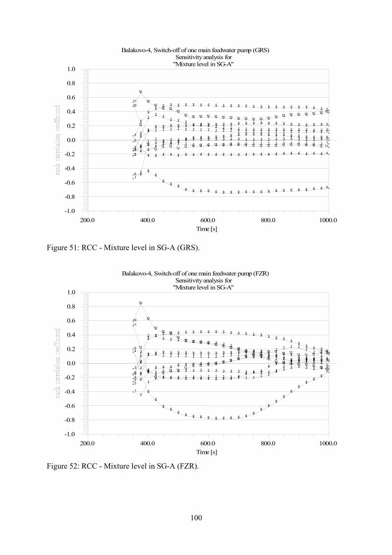
"Mixture level in SG-A"Sensitivity analysis for

Balakovo-4, Switch-off of one main feedwater pump (GRS)

Time [s]1000.0800.0600.0400.0200.0

1.0

0.8

0.6

0.4

0.2

0.0

-0.2

-0.4

-0.6

-0.8

-1.0

1 1

1 1 1 1 1 1 1 1 1 1 1 1 1 1 1 1 1 1 1 1 1 1 1 1 1

2

2

2 2 2

2 2 2 2 2 2 2 2 2 2 2 2 2 2 2 2 2 2 2 2 2 2

3 3 3 3 3 3 3 3 3 3 3 3 3 3 3 3 3 3 3 3 3 3 3 3 3 3 3

4

4

4 4 4 4 4 4 4 4 4 4 4 4 4 4 4 4 4 4 4 4 4 4 4 4 4

5

5

5 5

5 5 5 5 5 5 5 5 5 5 5 5 5 5 5 5 5 5 5 5 5 5 5

6 6 6

6 6

6 6 6 6 6 6 6 6 6 6 6 6 6 6 6 6 6 6 6 6 6 6

7

7

7 7 7 7 7 7 7 7 7 7 7 7 7 7 7 7 7 7 7 7 7 7 7 7 7

8 8 8

8 8 8 8 8 8 8 8 8 8 8 8 8 8 8 8 8 8 8 8 8 8 8 8

9

9 9

9 9 9 9 9 9 9 9 9 9 9 9 9 9 9 9 9 9 9 9 9 9 9 9

10

10

10 10

10 10 10

10 10 10 10 10 10 10 10 10 10 10 10 10 10 10 10 10 10 10 10

11

11

11 11

11 11 11 11 11 11 11 11 11 11 11 11 11 11 11 11 11 11 11 11 11 11 11

Figure 51: RCC - Mixture level in SG-A (GRS).

Figure 52: RCC - Mixture level in SG-A (FZR).

"Mixture level in SG-A"Sensitivity analysis for

Balakovo-4, Switch-off of one main feedwater pump (FZR)

Time [s]1000.0800.0600.0400.0200.0

1.0

0.8

0.6

0.4

0.2

0.0

-0.2

-0.4

-0.6

-0.8

-1.0

1 1

1 1 1 1 1 1 1 1 1 1 1 1 1 1 1 1 1

1 1

1 1 1 1 1 1

2

2

2 2 2 2 2 2 2 2 2 2 2 2

2 2 2 2

2 2 2 2 2 2 2 2 2 3 3

3 3 3 3 3 3 3 3 3 3 3 3 3 3 3 3 3 3 3 3 3 3 3 3 3

4

4

4 4 4 4 4 4 4 4 4 4 4 4 4

4 4 4 4

4 4 4 4 4 4 4 4

5

5

5 5 5 5 5 5 5 5 5 5 5 5 5 5 5 5 5 5 5 5 5

5 5 5 5 6

6

6

6

6 6

6 6 6 6 6 6 6 6 6 6 6

6 6

6 6

6 6

6 6

6 6

7

7

7 7 7 7 7 7 7 7 7 7 7 7 7 7 7 7 7 7 7 7 7 7

7 7 7

8 8

8 8 8 8 8 8 8 8 8 8 8 8 8 8 8 8 8 8 8 8 8 8 8 8 8

9

9

9 9 9 9 9 9 9 9 9 9 9 9 9 9 9 9 9 9 9

9 9 9 9 9 9

10

10

10

10 10 10

10 10 10 10 10 10 10 10 10

10 10 10

10 10 10 10 10 10 10 10 10

11

11

11 11

11 11 11 11 11 11 11 11 11 11 11 11 11 11 11 11 11 11 11 11 11 11 11

100

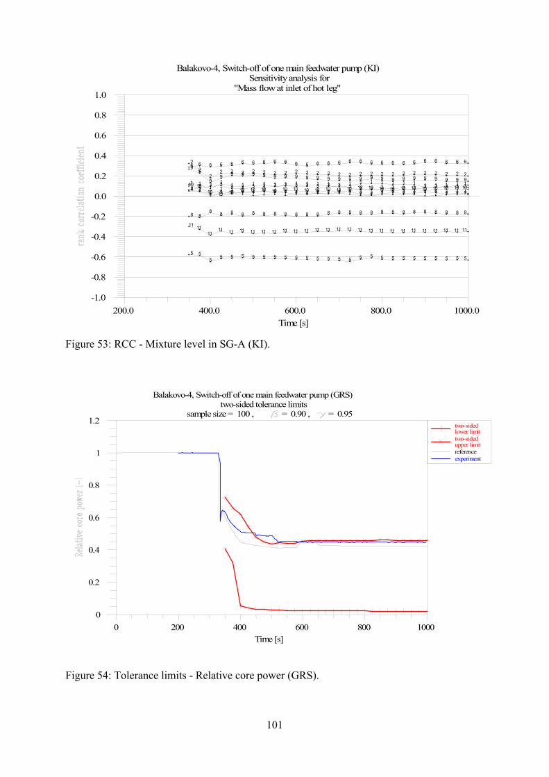
"Mass flow at inlet of hot leg"

Sensitivity analysis forBalakovo-4, Switch-off of one main feedwater pump (KI)

Time [s]1000.0800.0600.0400.0200.0

1.0

0.8

0.6

0.4

0.2

0.0

-0.2

-0.4

-0.6

-0.8

-1.0

1 1 1 1 1 1 1 1 1 1 1 1 1 1 1 1 1 1 1 1 1 1 1 1 1 1 1

2 2

2 2 2 2 2 2 2 2 2 2 2 2 2 2 2 2 2 2 2 2 2 2 2 2 2

3 3 3 3 3 3 3 3 3 3 3 3 3 3 3 3 3 3 3 3 3 3 3 3 3 3 3 4 4 4 4 4 4 4 4 4 4 4 4 4 4 4 4 4 4 4 4 4 4 4 4 4 4 4

5 5 5 5 5 5 5 5 5 5 5 5 5 5 5 5 5 5 5 5 5 5 5 5 5 5 5

6 6 6 6 6 6 6 6 6 6 6 6 6 6 6 6 6 6 6 6 6 6 6 6 6 6 6

7 7 7 7 7 7 7 7 7 7 7 7 7 7 7 7 7 7 7 7 7 7 7 7 7 7 7

8 8 8 8 8 8 8 8 8 8 8 8 8 8 8 8 8 8 8 8 8 8 8 8 8 8 8

9 9

9 9 9 9 9 9 9 9 9 9 9 9 9 9 9 9 9 9 9 9 9 9 9 9 9

10 10 10 10 10 10 10 10 10 10 10 10 10 10 10 10 10 10 10 10 10 10 10 10 10 10 10

11 11 11

11 11 11 11 11 11 11 11 11 11 11 11 11 11 11 11 11 11 11 11 11 11 11 11

Figure 53: RCC - Mixture level in SG-A (KI).

= 0.95 = 0.90 , sample size = 100 ,

two-sided tolerance limitsBalakovo-4, Switch-off of one main feedwater pump (GRS)

Time [s]10008006004002000

1.2

1

0.8

0.6

0.4

0.2

0

referenceexperiment

upper limittwo-sidedlower limittwo-sided

Figure 54: Tolerance limits - Relative core power (GRS).

101

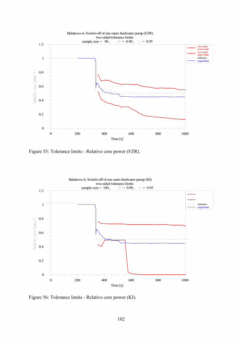
= 0.95 = 0.90 , sample size = 98 ,

two-sided tolerance limitsBalakovo-4, Switch-off of one main feedwater pump (FZR)

Time [s]10008006004002000

1.2

1

0.8

0.6

0.4

0.2

0

referenceexperiment

upper limittwo-sidedlower limittwo-sided

upper limittwo-sidedlower limittwo-sided

Figure 55: Tolerance limits - Relative core power (FZR).

Figure 56: Tolerance limits - Relative core power (KI).

= 0.95 = 0.90 , sample size = 100 ,

two-sided tolerance limitsBalakovo-4, Switch-off of one main feedwater pump (KI)

Time [s]10008006004002000

1.2

1

0.8

0.6

0.4

0.2

0

referenceexperiment

102

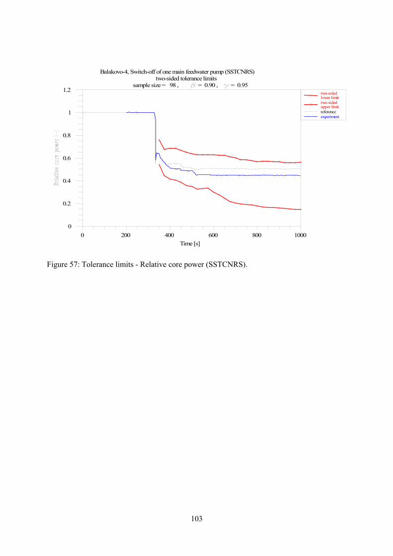
= 0.95 = 0.90 , sample size = 98 ,

two-sided tolerance limitsBalakovo-4, Switch-off of one main feedwater pump (SSTCNRS)

Time [s]10008006004002000

1.2

1

0.8

0.6

0.4

0.2

0

referenceexperiment

upper limittwo-sidedlower limittwo-sided

Figure 57: Tolerance limits - Relative core power (SSTCNRS).

103

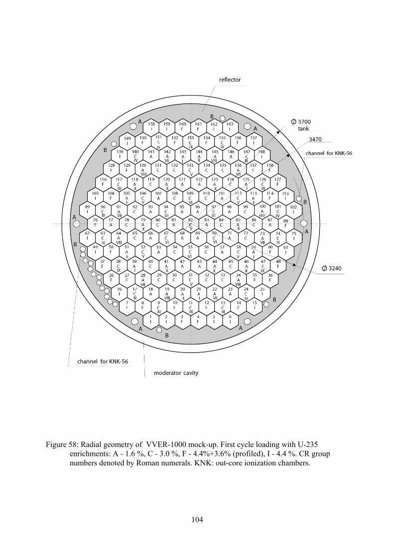
Figure 58: Radial geometry of VVER-1000 mock-up. First cycle loading with U-235 enrichments: A - 1.6 %, C - 3.0 %, F - 4.4%+3.6% (profiled), I - 4.4 %. CR group numbers denoted by Roman numerals. KNK: out-core ionization chambers.

104

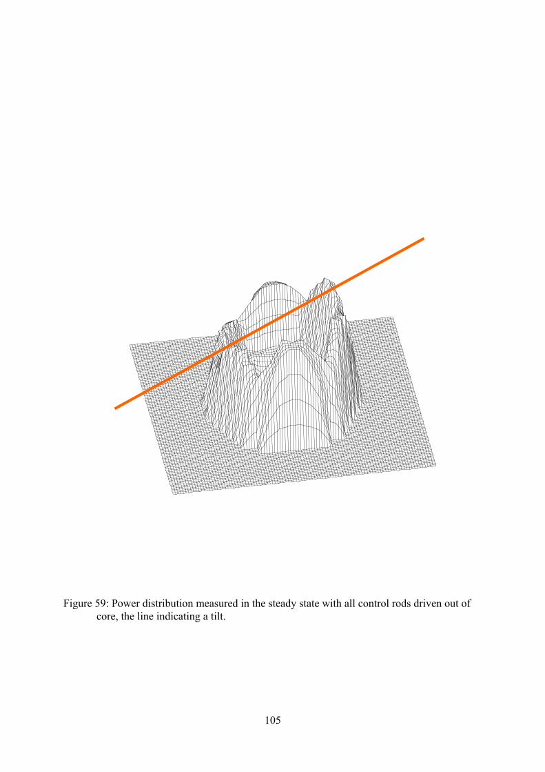
105

Figure 59: Power distribution measured in the steady state with all control rods driven out of core, the line indicating a tilt.

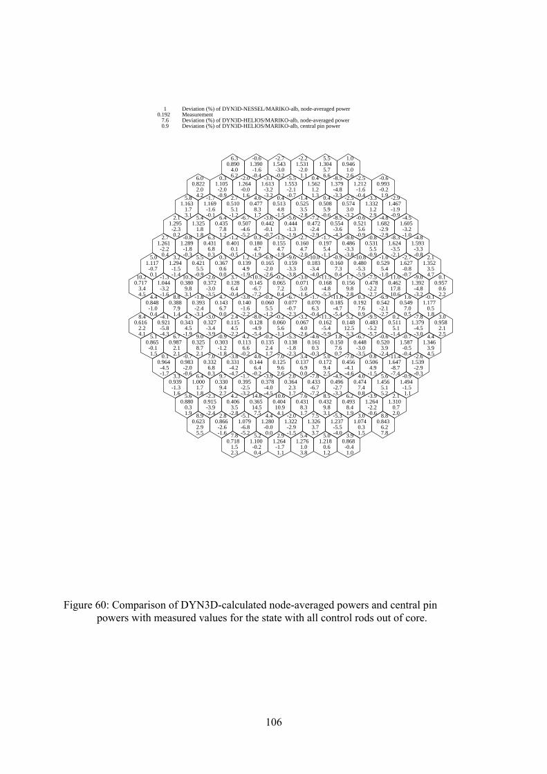
7.80.718 1.5 2.3

5.21.100 -0.2 0.4

2.91.264 -1.7 1.1

5.41.276 1.0 3.8

5.01.218 0.6 1.2

3.90.868 -0.4 1.0

8.90.623 2.9 5.5

2.80.866 -2.6 -1.6

-5.11.079 -6.8 -5.2

4.41.280 -0.0 0.0

-2.01.322 -2.9 -1.5

7.51.326 3.7 3.7

-5.31.237 -5.5 -4.0

3.01.074 0.3 1.5

8.80.843 6.2 7.8

5.60.880 0.3 1.9

-2.30.915 -3.9 -2.4

4.20.406 3.5 -2.8

14.80.365 14.5 7.5

10.60.404 10.9 4.1

7.60.431 8.3 1.7

8.50.432 9.8 3.1

6.20.493 8.4 1.9

-3.91.264 -2.2 -0.6

2.11.310 0.7 2.0

3.30.939 -1.3 1.6

6.41.000 1.7 1.8

9.70.330 9.4 2.7

-1.70.395 -2.5 -3.2

-3.90.378 -4.0 -4.5

2.00.364 2.3 1.7

-7.80.433 -6.7 -7.2

-4.50.496 -2.7 -3.3

4.00.474 7.4 0.8

5.61.456 5.1 5.2

-0.91.494 -1.5 1.1

0.10.964 -4.5 -1.7

-0.70.983 -2.0 -0.6

7.00.332 6.8 0.3

-3.80.331 -4.2 -4.7

4.60.144 6.4 -0.2

7.00.125 9.6 2.6

3.40.137 6.9 0.0

5.00.172 9.4 2.5

-7.00.456 -4.1 -4.6

0.80.506 4.9 -1.5

-11.41.647 -8.7 -7.4

-2.61.539 -2.9 -0.3

5.10.865 -0.1 1.5

6.70.987 2.1 2.1

9.00.325 8.7 2.1

-0.90.303 -1.2 -1.8

4.20.113 6.6 -0.2

-0.20.135 2.4 1.7

-5.30.138 -1.8 -2.3

-4.60.161 0.3 -0.3

1.80.150 7.6 0.7

-6.70.448 -3.0 -3.5

-0.60.520 3.9 -2.4

-0.71.587 -0.5 -0.4

4.41.346 3.9 4.5

8.40.616 2.2 4.1

-4.10.921 -5.8 -4.3

4.70.343 4.5 -1.9

-3.00.327 -3.4 -3.9

2.40.115 4.5 -2.2

-8.00.128 -4.9 -5.4

-0.20.060 5.6 -1.1

-3.20.067 4.0 -2.6

-11.30.162 -5.4 -5.9

5.20.148 12.5 5.3

-9.50.483 -5.2 -5.7

0.20.511 5.1 -1.4

-7.81.379 -4.5 -3.0

3.00.958 2.1 2.5

4.40.848 -1.0 0.4

8.80.388 7.9 1.4

-1.80.393 -2.4 -3.1

4.70.143 6.7 0.0

-3.80.140 -1.6 -2.2

-0.20.060 5.5 -1.2

-6.70.077 -0.7 -2.3

-1.70.070 6.3 -0.4

-11.00.185 -4.7 -5.4

0.30.192 7.6 0.9

-6.90.542 -2.1 -2.7

1.60.549 7.0 0.5

-0.11.177 0.5 1.8

10.20.717 3.4 4.5

-1.31.044 -3.2 -1.6

10.30.380 9.8 3.1

-2.60.372 -3.0 -3.5

3.70.128 6.4 -0.4

-10.50.145 -6.7 -7.2

-0.20.065 7.2 0.4

-3.00.071 5.0 -1.6

-11.50.168 -4.8 -5.3

1.70.156 9.8 2.8

-7.50.478 -2.2 -2.7

11.00.462 17.8 10.6

-9.01.392 -4.8 -3.2

0.10.957 0.6 2.2

5.01.117 -0.7 0.1

3.21.294 -1.5 -1.4

5.50.421 5.5 -0.9

0.30.367 0.6 0.0

1.20.139 4.9 -1.9

-6.90.165 -2.0 -2.6

-9.60.159 -3.3 -3.8

-10.00.183 -3.4 -4.0

-0.90.160 7.3 0.4

-10.80.480 -5.3 -5.9

-1.00.529 5.4 -1.0

-2.71.627 -0.8 -0.7

2.11.352 3.5 4.7

2.71.261 -2.2 0.4

-0.81.289 -1.8 -0.3

6.30.431 6.8 0.3

-1.20.401 0.1 -0.5

0.30.180 4.7 -1.9

-1.50.155 4.7 -1.9

-2.70.160 4.7 -2.0

-1.70.197 5.4 -1.1

-8.60.486 -3.3 -3.8

-0.80.531 5.5 -0.9

-8.31.624 -3.5 -2.1

-4.81.593 -3.3 -0.8

2.11.295 -2.3 0.2

5.41.325 1.8 1.8

6.40.435 7.8 1.2

-6.70.507 -4.6 -5.2

-3.60.442 -0.1 -0.7

-5.60.444 -1.3 -1.9

-7.20.472 -2.4 -2.9

-8.50.554 -3.6 -4.3

-0.60.521 5.6 -0.9

-4.81.682 -2.9 -2.9

-4.51.605 -3.2 -1.0

5.81.163 1.7 3.1

-1.71.169 -1.6 -0.1

2.70.510 5.1 -1.2

4.60.477 8.3 1.7

0.40.513 4.8 -1.5

-1.40.525 3.5 -2.8

0.40.508 5.9 -0.6

-2.50.574 3.0 -3.2

-3.31.332 1.2 2.9

-2.91.467 -1.9 -0.9

6.00.822 2.0 4.2

0.31.105 -2.0 -0.9

-2.01.264 -0.0 1.6

-3.11.613 -3.2 -3.2

-5.51.553 -2.1 -0.7

0.41.562 1.2 1.3

-8.51.379 -4.8 -3.3

-2.51.212 -1.6 -0.4

-0.60.993 -0.2 1.9

6.30.890 4.0 6.2

-0.61.390 -1.6 -0.4

-2.71.543 -3.0 -0.2

-2.21.531 -2.0 1.1

5.51.304 5.7 6.6

1.00.946 1.0 2.6

1 Deviation (%) of DYN3D-NESSEL/MARIKO-alb, node-averaged power0.192 Measurement 7.6 Deviation (%) of DYN3D-HELIOS/MARIKO-alb, node-averaged power 0.9 Deviation (%) of DYN3D-HELIOS/MARIKO-alb, central pin power

106

Figure 60: Comparison of DYN3D-calculated node-averaged powers and central pin powers with measured values for the state with all control rods out of core.

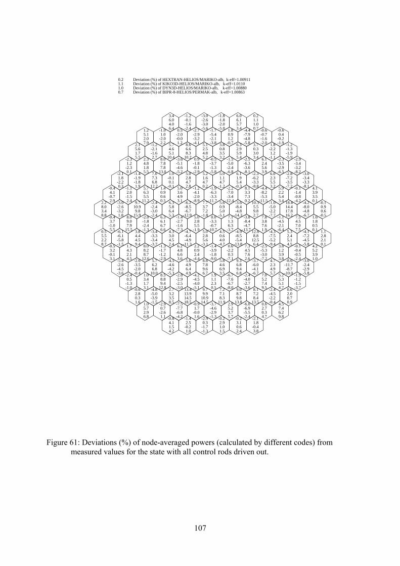
-0.8 4.1 1.5 4.2

-1.4 2.5 -0.2 1.0

-2.9 0.3 -1.7 -1.3

-0.2 2.9 1.0 1.5

-0.2 3.1 0.6 2.4

-2.1 1.8 -0.4 3.8

1.0 5.7 2.9 6.8

-2.9 0.7 -2.6 1.1

-7.5 -7.7 -6.8 -4.2

-0.9 1.7 -0.0 1.6

-3.7 -4.6 -2.9 -1.3

2.9 5.2 3.7 5.7

-6.0 -6.9 -5.5 -2.4

0.6 2.7 0.3 4.7

4.5 7.4 6.2 9.8

-0.6 2.8 0.3 1.6

-4.8 -5.0 -3.9 -1.5

2.7 3.2 3.5 8.5

13.4 13.9 14.5 18.5

9.7 9.9 10.9 14.5

7.2 7.1 8.3 11.9

9.0 8.7 9.8 13.8

8.1 7.2 8.4 13.5

-2.4 -4.5 -2.2 -0.4

0.6 2.0 0.7 0.9

-2.4 0.5 -1.3 -1.0

1.0 3.4 1.7 3.1

8.5 8.8 9.4 12.8

-2.8 -2.9 -2.5 -3.0

-4.2 -4.5 -4.0 -5.1

1.9 1.1 2.3 0.5

-6.7 -7.6 -6.7 -8.0

-2.4 -4.0 -2.7 -3.6

7.0 5.2 7.4 9.5

5.2 5.3 5.1 4.7

-1.9 -1.2 -1.5 -3.7

-5.4 -2.6 -4.5 -3.6

-2.6 -3.5 -2.0 -0.4

5.7 6.2 6.8 10.0

-4.5 -4.6 -4.2 -5.3

5.6 4.9 6.4 4.9

8.8 7.8 9.6 6.7

5.8 4.6 6.9 3.5

9.3 6.8 9.4 6.8

-3.7 -6.0 -4.1 -6.7

4.7 2.3 4.9 5.7

-8.6-11.7 -8.7-10.0

-3.0 -2.4 -2.9 -5.8

-0.5 3.2 -0.1 3.1

1.7 4.3 2.1 4.5

8.0 8.2 8.7 12.6

-1.3 -1.7 -1.2 -2.9

6.2 4.8 6.6 3.6

2.2 0.9 2.4 -4.4

-1.4 -3.9 -1.8 -9.0

0.6 -2.2 0.3 -7.1

7.3 4.5 7.6 2.6

-2.5 -5.3 -3.0 -7.2

3.8 1.2 3.9 3.8

-0.1 -0.4 -0.5 -2.4

4.2 5.2 3.9 1.0

0.5 5.5 2.2 8.7

-6.1 -6.1 -5.8 -1.5

3.8 4.4 4.5 9.4

-3.4 -3.3 -3.4 -3.7

4.3 3.0 4.5 2.4

-4.7 -6.4 -4.9-11.3

5.0 2.8 5.6 -3.1

4.5 0.6 4.0 -4.7

-4.9 -8.5 -5.4-13.8

12.8 8.8 12.5 6.4

-4.3 -7.5 -5.2 -9.4

5.3 2.4 5.1 4.5

-4.1 -7.2 -4.5 -5.8

1.1 2.8 2.1 0.1

-0.4 3.7 -1.0 5.5

8.0 9.0 7.9 15.5

-2.0 -1.8 -2.4 -1.3

6.3 6.1 6.7 6.6

-1.4 -2.7 -1.6 -7.3

5.0 2.8 5.5 -1.9

0.0 -3.3 -0.7-10.7

7.1 1.3 6.3 -3.7

-3.8 -8.4 -4.7-13.7

7.8 3.8 7.6 1.9

-1.1 -4.5 -2.1 -6.4

7.5 4.5 7.0 7.5

1.6 1.8 0.5 0.1

2.2 8.0 3.4 8.8

-3.0 -2.6 -3.2 1.8

9.7 10.9 9.8 15.9

-2.4 -2.4 -3.0 -2.4

6.3 5.8 6.4 5.3

-6.2 -8.5 -6.7-12.9

7.7 3.7 7.2 -1.8

5.6 0.9 5.0 -5.1

-3.6 -8.4 -4.8-14.3

10.3 5.5 9.8 2.7

-1.0 -5.0 -2.2 -7.7

18.4 14.4 17.8 16.2

-4.2 -8.0 -4.8 -6.7

-0.1 0.9 0.6 -0.5

-0.4 4.1 -0.7 2.9

-1.1 2.0 -1.5 2.4

5.7 6.3 5.5 11.2

1.4 0.9 0.6 0.5

5.0 3.6 4.9 3.1

-1.2 -4.1 -2.0 -8.9

-1.9 -6.3 -3.3-11.7

-2.2 -7.0 -3.4-12.4

8.1 3.3 7.3 0.2

-4.4 -8.2 -5.3-11.5

5.9 2.2 5.4 3.4

-0.1 -1.4 -0.8 -4.2

4.1 3.9 3.5 0.1

-2.1 1.8 -2.2 0.3

-1.4 -1.9 -1.8 1.9

7.0 7.3 6.8 12.2

1.0 -0.1 0.1 -0.1

5.0 2.8 4.7 2.8

5.2 1.6 4.7 0.2

5.0 1.1 4.7 -1.2

6.1 1.9 5.4 -0.3

-2.3 -6.2 -3.3 -8.8

6.0 2.3 5.5 3.2

-2.8 -7.2 -3.5 -7.2

-3.0 -3.4 -3.3 -8.1

-2.3 1.2 -2.3 0.1

2.3 4.8 1.8 5.5

8.0 7.8 7.8 13.0

-3.6 -5.1 -4.6 -5.2

0.9 -1.8 -0.1 -2.9

-0.5 -3.7 -1.3 -5.8

-1.5 -5.0 -2.4 -6.8

-2.5 -6.3 -3.6 -8.1

6.1 2.4 5.6 3.9

-2.3 -3.5 -2.9 -6.5

-2.9 -3.4 -3.2 -8.2

2.1 5.6 1.7 5.5

-1.2 -2.1 -1.6 2.7

5.7 4.6 5.1 10.4

8.6 6.6 8.3 10.2

5.1 2.5 4.8 5.2

3.8 0.8 3.5 3.2

6.3 2.9 5.9 5.4

3.7 0.3 3.0 3.4

1.8 -2.2 1.2 -1.1

-1.2 -1.3 -1.9 -5.9

1.2 5.1 2.0 7.9

-1.0 1.0 -2.0 2.2

0.5 -2.0 -0.0 1.2

-2.7 -2.9 -3.2 -4.1

-1.7 -5.4 -2.1 -3.8

1.8 0.9 1.2 -0.7

-4.4 -7.9 -4.8 -5.8

-0.6 -0.7 -1.6 -2.0

-0.6 0.4 -0.2 -1.9

3.4 6.0 4.0 6.4

-1.2 -0.1 -1.6 -2.4

-3.0 -2.6 -3.0 -5.6

-1.8 -1.8 -2.0 -5.0

6.0 6.1 5.7 3.4

0.2 1.1 1.0 0.7

0.2 Deviation (%) of HEXTRAN-HELIOS/MARIKO-alb, k-eff=1.00911 1.1 Deviation (%) of KIKO3D-HELIOS/MARIKO-alb, k-eff=1.0110 1.0 Deviation (%) of DYN3D-HELIOS/MARIKO-alb, k-eff=1.00880 0.7 Deviation (%) of BIPR-8-HELIOS/PERMAK-alb, k-eff=1.00863

107

Figure 61: Deviations (%) of node-averaged powers (calculated by different codes) from measured values for the state with all control rods driven out.

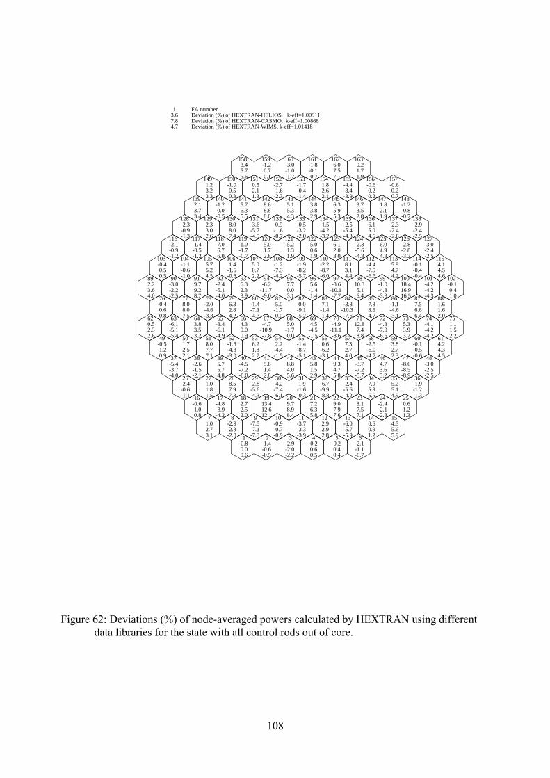
1 -0.8 0.0 0.6

2 -1.4 -0.6 -0.5

3 -2.9 -2.0 -2.2

4 -0.2 0.6 0.5

5 -0.2 0.4 0.4

6 -2.1 -1.1 -0.7

7 1.0 2.7 3.1

8 -2.9 -2.3 -2.0

9 -7.5 -7.1 -7.3

10 -0.9 -0.7 -0.9

11 -3.7 -3.3 -3.9

12 2.9 2.9 2.8

13 -6.0 -5.7 -5.9

14 0.6 0.9 1.2

15 4.5 5.6 5.9

16 -0.6 1.0 0.8

17 -4.8 -3.9 -4.2

18 2.7 2.5 2.0

19 13.4 12.6 12.1

20 9.7 8.9 8.4

21 7.2 6.3 5.8

22 9.0 7.9 7.6

23 8.1 7.5 7.1

24 -2.4 -2.1 -2.3

25 0.6 1.2 1.3

26 -2.4 -0.6 -1.1

27 1.0 1.8 1.5

28 8.5 7.9 7.3

29 -2.8 -5.6 -4.3

30 -4.2 -7.4 -6.1

31 1.9 -1.6 -0.3

32 -6.7 -9.9 -8.8

33 -2.4 -5.6 -4.2

34 7.0 5.9 5.5

35 5.2 5.1 4.9

36 -1.9 -1.2 -1.3

37 -5.4 -3.7 -4.0

38 -2.6 -1.5 -2.1

39 5.7 5.7 4.8

40 -4.5 -7.2 -6.0

41 5.6 1.4 2.8

42 8.8 4.0 5.6

43 5.8 1.5 2.9

44 9.3 4.7 5.8

45 -3.7 -7.2 -5.7

46 4.7 3.6 3.2

47 -8.6 -8.5 -8.9

48 -3.0 -2.5 -2.5

49 -0.5 1.2 0.9

50 1.7 2.5 2.1

51 8.0 7.7 7.1

52 -1.3 -4.3 -3.0

53 6.2 1.8 2.7

54 2.2 -4.4 -1.5

55 -1.4 -8.7 -5.1

56 0.6 -6.2 -3.1

57 7.3 2.7 4.0

58 -2.5 -6.0 -4.7

59 3.8 2.7 2.3

60 -0.1 -0.5 -0.6

61 4.2 4.3 4.5

62 0.5 2.3 2.6

63 -6.1 -5.1 -5.4

64 3.8 3.5 3.2

65 -3.4 -6.1 -4.9

66 4.3 0.0 0.9

67 -4.7-10.9 -7.8

68 5.0 -1.7 0.0

69 4.5 -4.5 -1.5

70 -4.9-11.1 -8.6

71 12.8 7.4 8.8

72 -4.3 -7.9 -6.6

73 5.3 3.9 3.7

74 -4.1 -4.2 -4.2

75 1.1 1.5 2.2

76 -0.4 0.6 0.8

77 8.0 8.0 7.5

78 -2.0 -4.6 -3.3

79 6.3 2.8 4.2

80 -1.4 -7.1 -4.3

81 5.0 -1.7 0.0

82 0.0 -9.1 -5.2

83 7.1 -1.4 1.4

84 -3.8-10.3 -7.6

85 7.8 3.6 4.7

86 -1.1 -4.6 -3.1

87 7.5 6.6 6.4

88 1.6 1.6 2.0

89 2.2 3.6 4.0

90 -3.0 -2.2 -2.5

91 9.7 9.2 8.7

92 -2.4 -5.1 -4.0

93 6.3 2.3 3.9

94 -6.2-11.7 -9.0

95 7.7 0.0 3.1

96 5.6 -1.4 1.4

97 -3.6-10.1 -7.7

98 10.3 5.1 6.4

99 -1.0 -4.8 -3.3

100 18.4 16.9 16.5

101 -4.2 -4.2 -4.3

102 -0.1 0.4 1.0

103 -0.4 0.5 0.5

104 -1.1 -0.6 -1.0

105 5.7 5.2 4.5

106 1.4 -1.6 -0.3

107 5.0 0.7 2.2

108 -1.2 -7.3 -4.2

109 -1.9 -8.2 -5.7

110 -2.2 -8.7 -6.0

111 8.1 3.1 4.4

112 -4.4 -7.9 -6.5

113 5.9 4.7 4.2

114 -0.1 -0.4 -0.4

115 4.1 4.5 4.6

116 -2.1 -0.9 -1.2

117 -1.4 -0.5 -1.2

118 7.0 6.7 6.0

119 1.0 -1.7 -0.7

120 5.0 1.7 2.8

121 5.2 1.3 1.9

122 5.0 0.6 1.9

123 6.1 2.0 3.0

124 -2.3 -5.6 -4.3

125 6.0 4.9 4.3

126 -2.8 -2.8 -3.2

127 -3.0 -2.4 -2.5

128 -2.3 -0.9 -1.3

129 2.3 3.0 2.6

130 8.0 8.0 7.4

131 -3.6 -5.7 -4.9

132 0.9 -1.6 -0.7

133 -0.5 -3.2 -2.0

134 -1.5 -4.2 -3.2

135 -2.5 -5.4 -4.3

136 6.1 5.0 4.6

137 -2.3 -2.4 -2.6

138 -2.9 -2.4 -2.5

139 2.1 3.7 3.4

140 -1.2 0.0 -0.5

141 5.7 6.3 5.5

142 8.6 8.8 8.0

143 5.1 5.3 4.3

144 3.8 3.8 2.9

145 6.3 5.9 5.3

146 3.7 3.5 2.8

147 1.8 2.1 1.9

148 -1.2 -0.8 -0.7

149 1.2 3.2 3.3

150 -1.0 0.5 0.3

151 0.5 2.1 1.3

152 -2.7 -1.6 -2.3

153 -1.7 -0.4 -1.4

154 1.8 2.6 2.1

155 -4.4 -3.4 -3.9

156 -0.6 0.2 0.2

157 -0.6 0.2 0.7

158 3.4 5.7 5.6

159 -1.2 0.7 0.1

160 -3.0 -1.0 -1.7

161 -1.8 -0.1 -0.7

162 6.0 7.5 7.1

163 0.2 1.7 1.9

1 FA number 3.6 Deviation (%) of HEXTRAN-HELIOS, k-eff=1.00911 7.8 Deviation (%) of HEXTRAN-CASMO, k-eff=1.00868 4.7 Deviation (%) of HEXTRAN-WIMS, k-eff=1.01418

108

Figure 62: Deviations (%) of node-averaged powers calculated by HEXTRAN using different data libraries for the state with all control rods out of core.

- - - - - -

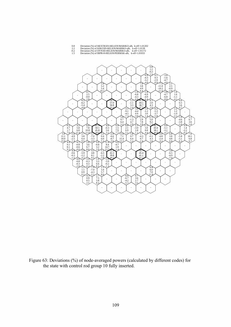
-4.3 0.9 0.5 2.5

2.7 7.5 5.8 8.3

- - -6.6 -6.7 -4.2 -5.7

0.7 3.6 2.7 3.5

- - -

-3.1 1.1 0.9 0.1

-7.9 -7.4 -4.3 -5.1

2.1 3.4 5.7 8.6

- - - - 6.4 6.0 7.0 11.8

- -

-4.6 -0.8 -0.3 -2.0

-3.4 -0.3 0.3 -0.2

2.4 3.3 6.6 8.1

-2.8 -3.9 -0.2 -1.3

- - - - - - -

-4.4 -0.6 -0.3 -1.5

-5.9 -5.9 -2.2 -4.2

4.1 4.8 8.1 9.5

-5.1 -6.5 -2.2 -3.8

35.4 42.3 39.8 49.5

- - 39.7 45.4 41.1 52.2

- - -3.8 -6.5 -4.9 -7.0

-

4.4 9.1 8.1 9.3

-4.1 -0.8 -0.6 -0.0

2.8 3.6 6.7 8.6

0.0 -0.8 3.2 2.0

11.4 8.4 14.7 13.7

0.0 -4.7 1.9 -1.4

- - - - - - -

5.0 11.1 10.0 15.0

-5.6 -4.9 -2.5 -1.4

2.7 3.8 6.4 9.5

-5.7 -7.0 -3.3 -4.0

3.2 0.4 6.0 5.3

-2.0 -6.6 -0.7 -3.6

13.6 7.1 15.4 13.7

5.8 0.7 6.4 5.2

1.7 -4.3 0.7 -2.4

6.1 -0.1 4.3 3.0

0.0 -4.8 -2.4 -4.2

6.6 3.8 4.8 6.0

-3.1 -5.8 -5.1 -6.3

7.6 10.1 6.8 6.7

-0.2 4.7 1.7 7.0

4.2 5.8 6.8 12.4

8.8 7.8 10.8 11.6

41.9 50.1 45.8 58.6

4.0 -0.3 5.6 3.1

6.4 1.5 7.9 7.7

8.8 2.1 6.9 5.1

5.3 -3.0 2.8 1.1

11.5 3.0 8.8 4.4

40.7 43.4 38.1 46.8

0.0 -5.1 -3.1 -4.7

- 0.9 1.4 -2.2 -0.2

- - - - - - 5.8 0.7 6.4 5.2

7.1 -1.3 4.7 2.9

11.1 2.9 7.8 3.9

12.5 5.0 9.2 7.3

- - -1.0 -4.6 -3.8 -5.0

5.3 6.7 3.6 5.0

- - - - - - -3.1 -9.1 -4.5 -7.3

3.8 -4.4 0.9 -3.0

5.9 -1.2 3.0 1.4

-0.2 -5.3 -3.7 -5.8

- 2.2 1.2 -1.0 -2.1

-

- -6.5 -6.2 -5.4 -4.9

- - 50.7 57.0 50.8 63.4

- 5.3 -1.1 3.3 2.4

41.9 44.1 38.7 47.5

8.1 2.0 4.3 2.0

- - 6.6 6.5 3.6 0.7

- -0.7 2.5 -0.0 2.8

- - - - -1.6 -6.8 -4.3 -6.0

-1.8 -6.9 -4.9 -6.4

- -3.8 -4.7 -6.8 -8.0

1.6 1.6 -1.1 -4.1

- - 5.9 5.2 5.4 10.7

- - - 7.0 3.8 4.9 6.4

- -7.5-11.0-10.2-11.6

2.1 2.5 -0.9 -2.8

- - - - - - -0.9 -4.3 -3.2 -4.0

0.1 0.3 -2.9 -0.9

-3.0 -1.6 -4.7 -4.0

- - - - - 0.8 2.2 -0.2 1.5

0.8 Deviation (%) of HEXTRAN-HELIOS/MARIKO-alb, k-eff=1.01202 2.2 Deviation (%) of KIKO3D-HELIOS/MARIKO-alb, k-eff=1.0139 -0.2 Deviation (%) of DYN3D-HELIOS/MARIKO-alb, k-eff=1.01172 1.5 Deviation (%) of BIPR-8-HELIOS/PERMAK-alb, k-eff=1.01033

109

Figure 63: Deviations (%) of node-averaged powers (calculated by different codes) for the state with control rod group 10 fully inserted.

- - - - - -

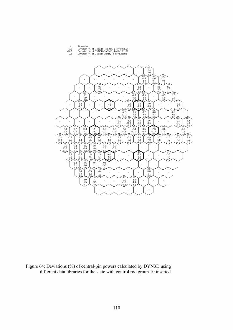
7 3.0 6.5 5.7

8 7.1 9.5 8.8

- - 11

-2.5 -3.0 -3.5

12 3.0 4.4 3.3

- - -

16 2.6 5.8 4.5

17 -2.5 -2.2 -2.6

18 -0.4 -1.7 -0.6

- - - - 23 0.8 -1.1 0.3

- -

26 2.8 6.1 4.8

27 0.6 3.0 1.6

28 0.4 -1.1 0.1

29 -0.6 -3.5 -2.2

- - - - - - -

37 2.8 6.0 4.7

38 -0.5 -0.1 -0.8

39 1.9 0.5 1.6

40 -2.4 -5.4 -4.1

41 -6.1 -8.6 -8.0

- - 44

-5.3 -8.3 -7.5

- - 47

-3.3 -4.4 -4.5

-

49 9.9 13.2 11.9

50 -0.4 1.9 0.6

51 0.5 -0.8 0.2

52 2.9 -0.4 0.9

53 7.8 2.2 5.5

54 1.7 -5.6 -2.6

- - - - - - -

62 12.1 15.6 14.8

63 -0.7 -0.5 -0.8

64 0.1 -1.4 -0.2

65 -3.5 -6.5 -5.1

66 -0.3 -5.5 -2.5

67 -1.0 -8.1 -5.0

68 8.4 -0.9 3.9

69 -0.0 -8.8 -4.3

70 0.4 -7.4 -4.0

71 -1.9 -7.9 -4.6

72 -2.7 -6.8 -5.1

73 -1.3 -4.2 -2.5

74 -3.3 -4.6 -4.4

75 7.3 8.6 8.7

76 3.4 5.8 5.1

77 0.7 -0.6 0.6

78 10.4 7.1 8.6

79 -2.1 -4.7 -4.0

80 5.3 -2.1 1.0

81 1.3 -7.3 -2.8

82 5.5 -4.8 -0.2

83 -3.4-12.0 -7.6

84 8.5 -0.0 3.5

85 -7.3-10.7 -9.6

86 -3.6 -7.5 -5.7

- 88

-0.7 0.2 0.1

- - - - - - 95

-0.0 -8.5 -4.1

96 -1.6-10.1 -5.7

97 7.5 -0.9 2.7

98 2.6 -3.6 -0.1

- -101 -2.0 -3.3 -3.0

102 5.4 7.0 7.0

- - - - - -109 -4.8-11.7 -8.7

110 0.6 -7.0 -3.8

111 -3.2 -9.0 -5.8

112 -4.0 -8.3 -6.6

-114 -0.8 -0.1 -0.8

-

-117 -3.8 -4.2 -4.6

- -120 1.3 -1.5 -0.8

-122 -2.9 -8.1 -5.1

123 -6.8 -9.9 -8.9

124 4.0 -0.3 1.6

- -127 6.5 7.8 7.3

-129 0.2 1.9 0.8

- - - -134 -4.5 -7.9 -6.4

135 -5.3 -8.8 -7.2

-137 -6.5 -5.9 -6.5

138 1.3 2.5 2.0

- -141 -0.7 -2.0 -0.8

- - -145 -1.2 -3.3 -1.9

-147 -8.5 -9.5 -9.3

148 0.2 1.5 1.0

- - - - - -155 -1.4 -2.0 -2.0

156 -1.6 -0.1 -0.4

157 -2.7 -0.9 -1.0

- - - - -163 1.4 3.6 3.3

1 FA number -7.3 Deviation (%) of DYN3D-HELIOS, k-eff=1.01172-10.7 Deviation (%) of DYN3D-CASMO, k-eff=1.01132 -9.6 Deviation (%) of DYN3D-WIMS, k-eff=1.01692

110

Figure 64: Deviations (%) of central-pin powers calculated by DYN3D using different data libraries for the state with control rod group 10 inserted.

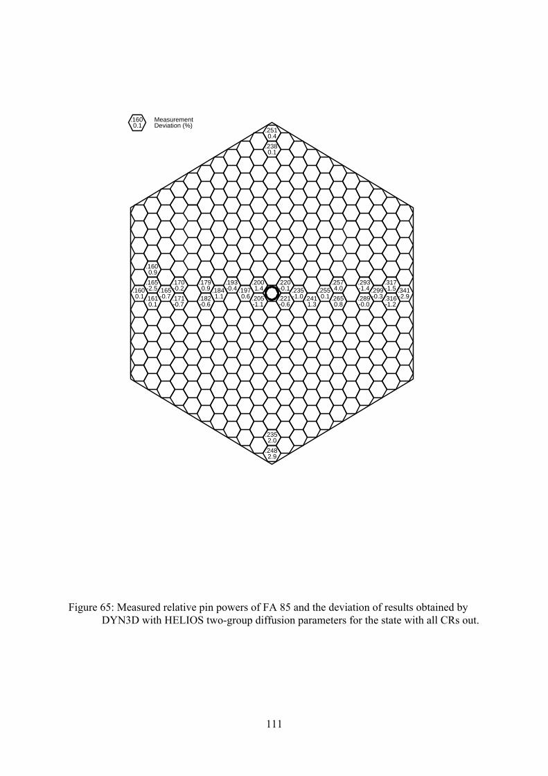
.160 0.1 .161

0.1

.165-2.5

.160 0.9

.165-0.7 .171

-0.7

.170-0.2

.182-0.6

.179 0.9 .184

1.1

.193-0.4 .197

0.6 .205-1.1

.200 1.4

.248 2.9

.235 2.0

.238 0.1

.251 0.4

.221-0.6

.220-0.1 .235

-1.0 .241 1.3

.255 0.1 .265

0.8

.257 4.0

.289-0.0

.293-1.4 .299

-0.3 .316-1.2

.317-1.5 .341

-2.9

.160 Measurement 0.1 Deviation (%)

111

Figure 65: Measured relative pin powers of FA 85 and the deviation of results obtained by DYN3D with HELIOS two-group diffusion parameters for the state with all CRs out.

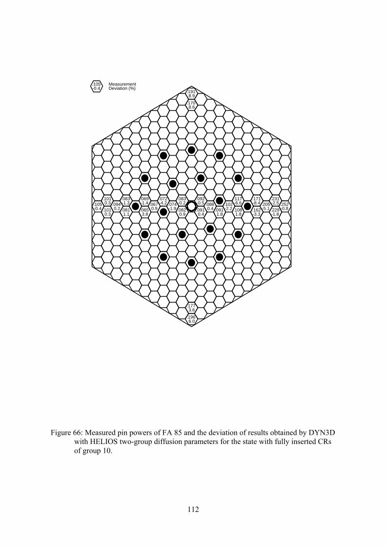
.105-0.4 .101

0.3

.101 0.3 .094

0.2 .081 1.1

.083-1.3

.065 3.8

.069-1.4 .067

0.9

.072-4.2 .074

-1.9 .082 0.9

.083-0.2

.196 6.0

.177 3.6

.170 8.6

.191 8.9

.091 0.4

.092-0.5 .088

0.4 .091 1.8

.102-2.2 .108

1.8

.117-6.6

.162-3.3

.171-8.4 .205

-5.1 .229-1.8

.231-2.5 .252

-0.8

.105 Measurement-0.4 Deviation (%)

Figure 66: Measured pin powers of FA 85 and the deviation of results obtained by DYN3D with HELIOS two-group diffusion parameters for the state with fully inserted CRs of group 10.

112

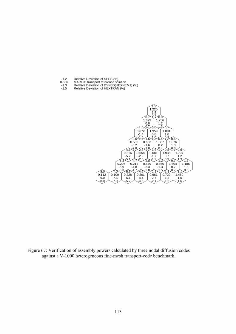
-8.0 0.112 -9.0 -8.0

-7.0 0.100 -7.5 -7.0

-5.3 0.228 -6.1 -5.7

-4.2 0.261 -4.4 -4.6

-2.1 0.661 -2.7 -2.1

-1.1 0.729 -1.3 -1.2

1.1 1.460 1.0 1.6

-6.3 0.207 -6.9 -6.3

-4.7 0.215 -4.8 -4.7

-2.8 0.579 -3.3 -2.8

-1.2 0.666 -1.3 -1.5

0.7 1.604 0.7 0.7

1.3 1.185 1.8 0.5

-4.6 0.216 -5.2 -5.1

-2.3 0.558 -2.9 -2.5

-1.6 0.681 -1.7 -1.9

0.8 1.938 0.7 0.9

0.9 1.707 1.2 1.3

-2.6 0.580 -3.2 -2.8

-1.5 0.683 -1.6 -1.8

0.4 1.887 0.2 0.4

0.6 1.876 1.0 0.8

-1.3 0.672 -1.4 -1.5

0.9 1.959 0.8 1.0

0.7 1.891 1.0 0.8

0.7 1.629 0.6 0.7

0.9 1.756 1.2 1.3

1.2 1.220 1.8 0.7

-1.2 Relative Deviation of SPPS (%) 0.666 MARIKO transport reference solution -1.3 Relative Deviation of DYN3D(HEXNEM1) (%) -1.5 Relative Deviation of HEXTRAN (%)

Figure 67: Verification of assembly powers calculated by three nodal diffusion codes against a V-1000 heterogeneous fine-mesh transport-code benchmark.

113

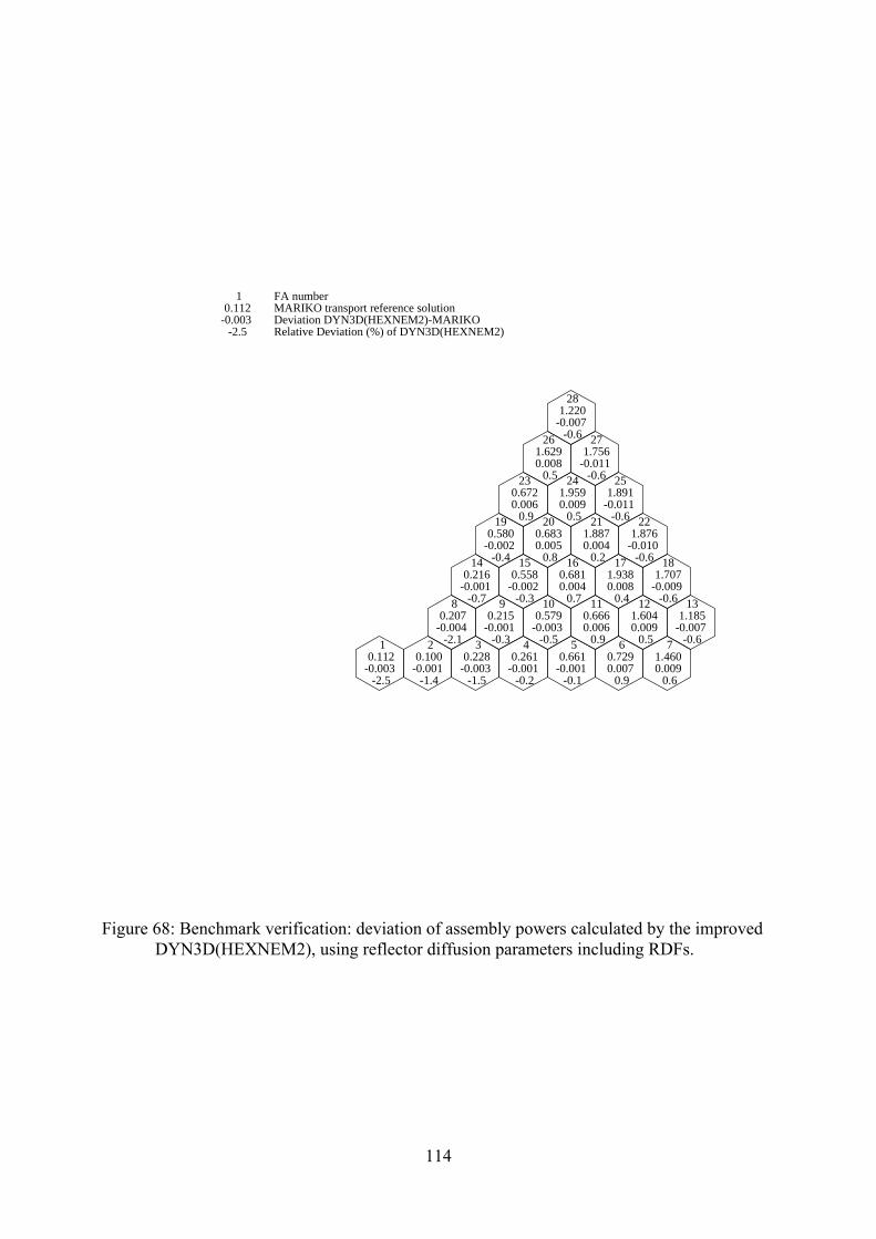
1 0.112-0.003 -2.5

2 0.100-0.001 -1.4

3 0.228-0.003 -1.5

4 0.261-0.001 -0.2

5 0.661-0.001 -0.1

6 0.729 0.007 0.9

7 1.460 0.009 0.6

8 0.207-0.004 -2.1

9 0.215-0.001 -0.3

10 0.579-0.003 -0.5

11 0.666 0.006 0.9

12 1.604 0.009 0.5

13 1.185-0.007 -0.6

14 0.216-0.001 -0.7

15 0.558-0.002 -0.3

16 0.681 0.004 0.7

17 1.938 0.008 0.4

18 1.707-0.009 -0.6

19 0.580-0.002 -0.4

20 0.683 0.005 0.8

21 1.887 0.004 0.2

22 1.876-0.010 -0.6

23 0.672 0.006 0.9

24 1.959 0.009 0.5

25 1.891-0.011 -0.6

26 1.629 0.008 0.5

27 1.756-0.011 -0.6

28 1.220-0.007 -0.6

1 FA number 0.112 MARIKO transport reference solution-0.003 Deviation DYN3D(HEXNEM2)-MARIKO -2.5 Relative Deviation (%) of DYN3D(HEXNEM2)

Figure 68: Benchmark verification: deviation of assembly powers calculated by the improved DYN3D(HEXNEM2), using reflector diffusion parameters including RDFs.

114

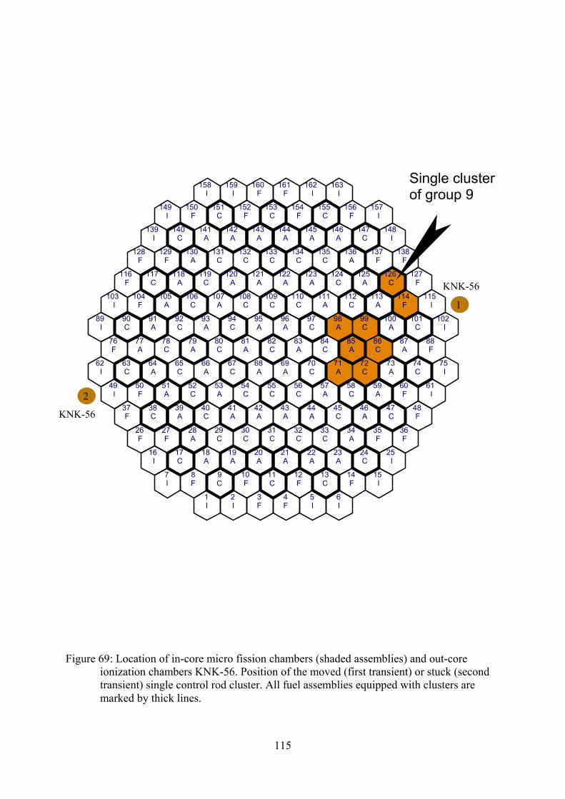
Single cluster of group 9

KNK-56 2

KNK-56

1

I163

I162

F161

F160

I157

F156

C155

F154

C153

F152

I148

C147

A146

A145

A144

A143

F137

A136

C135

C134

C133

C132

C126

A125

C124

A123

A122

A121

A113

C112

A111

C110

C109

C108

A100

C99

A98

C97

A96

A95

C86

A85

C84

A83

C82

A81

A73

C72

A71

C70

A69

A68

A59

C58

A57

C56

C55

C54

C47

A46

C45

A44

A43

A42

F 36

F 48

F 60

I 61

C 74

I 75

A 87

F 88

C 101

I 102

F 114

I 115

F 127

F 138

F35

A34

C33

C32

C31

C30

I25

C24

A23

A22

A21

A20

I 16

F 26

F 37

C 38

I 49

F 50

I 62

C 63

A 64

F 76

A 77

I 89

C 90

A 91

I 103

F 104

F 116

C 117

F 128

I 139

I149

F129

A105

C78

A51

F27

I15

F14

C13

F12

C11

F10

I7

I6

I5

F4

F3

I 1

F 8

C 9

C 17

A 18

A 28

C 29

A 39

C 40

C 52

A 53

C 65

A 66

A 79

C 80

C 92

A 93

C 106

A 107

A 118

C 119

A 130

C 131

C 140

A 141

F 150

C 151

I159

I 158

A142

A120

C94

C67

A41

A19

I2

Figure 69: Location of in-core micro fission chambers (shaded assemblies) and out-core ionization chambers KNK-56. Position of the moved (first transient) or stuck (second transient) single control rod cluster. All fuel assemblies equipped with clusters are marked by thick lines.

115

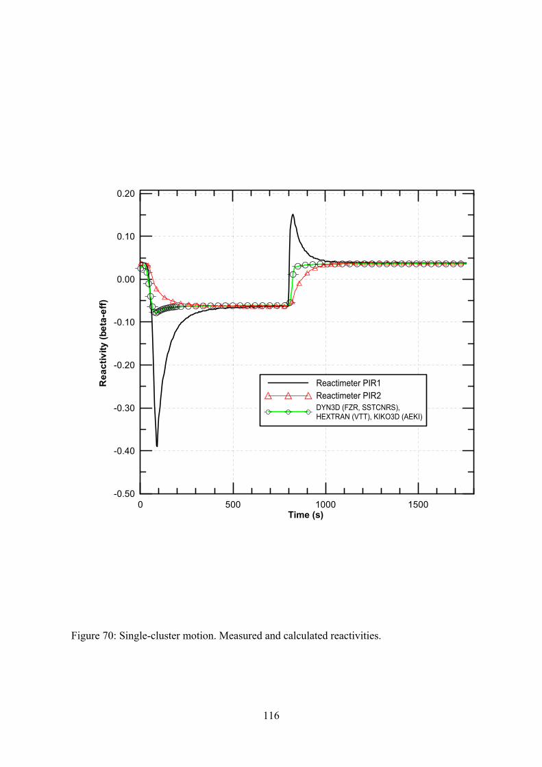
0 500 1000 1500Time (s)

-0.50

-0.40

-0.30

-0.20

-0.10

0.00

0.10

0.20

Rea

ctiv

ity (b

eta-

eff)

Reactimeter PIR1Reactimeter PIR2DYN3D (FZR, SSTCNRS),HEXTRAN (VTT), KIKO3D (AEKI)

Figure 70: Single-cluster motion. Measured and calculated reactivities.

116

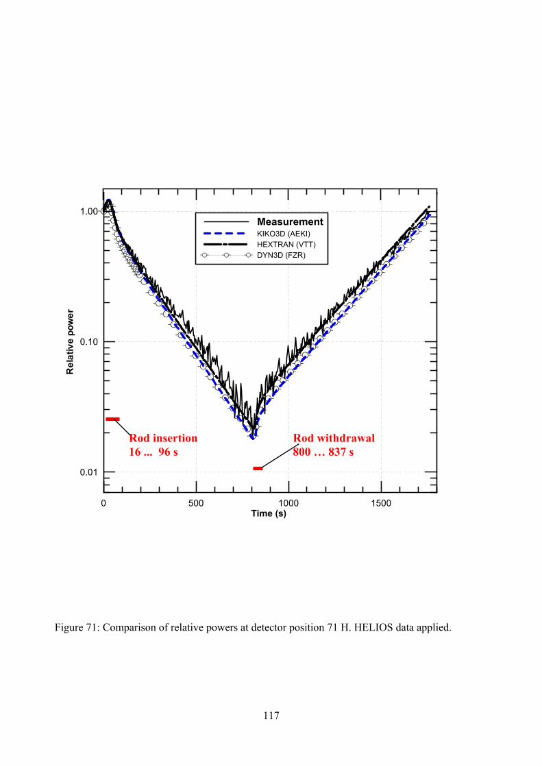
0 500 1000 1500Time (s)

0.01

0.10

1.00

Rel

ativ

e po

wer

MeasurementKIKO3D (AEKI)HEXTRAN (VTT)DYN3D (FZR)

Rod withdrawal 800 … 837 s

Rod insertion 16 ... 96 s

Figure 71: Comparison of relative powers at detector position 71 H. HELIOS data applied.

117

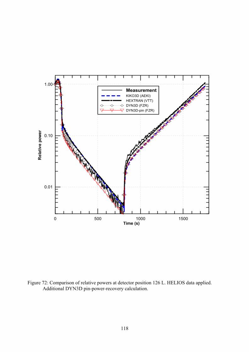
0 500 1000 1500Time (s)

0.01

0.10

1.00

Rel

ativ

e po

wer

MeasurementKIKO3D (AEKI)HEXTRAN (VTT)DYN3D (FZR)DYN3D-pin (FZR)

Figure 72: Comparison of relative powers at detector position 126 L. HELIOS data applied. Additional DYN3D pin-power-recovery calculation.

118

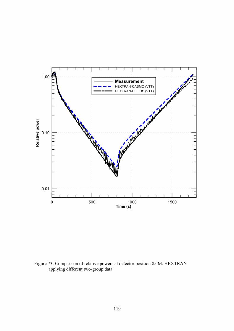
0 500 1000 1500Time (s)

0.01

0.10

1.00

Rel

ativ

e po

wer

MeasurementHEXTRAN-CASMO (VTT)HEXTRAN-HELIOS (VTT)

Figure 73: Comparison of relative powers at detector position 85 M. HEXTRAN applying different two-group data.

119

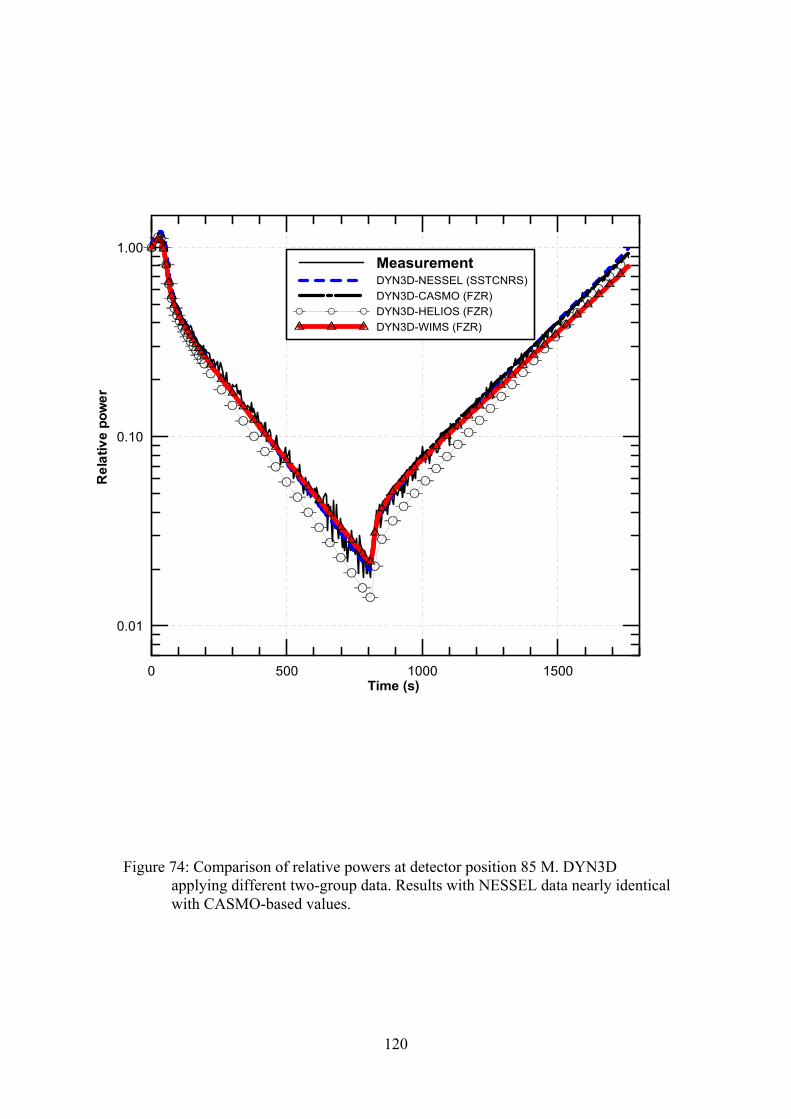
0 500 1000 1500Time (s)

0.01

0.10

1.00

Rel

ativ

e po

wer

MeasurementDYN3D-NESSEL (SSTCNRS)DYN3D-CASMO (FZR)DYN3D-HELIOS (FZR)DYN3D-WIMS (FZR)

Figure 74: Comparison of relative powers at detector position 85 M. DYN3D applying different two-group data. Results with NESSEL data nearly identical with CASMO-based values.

120

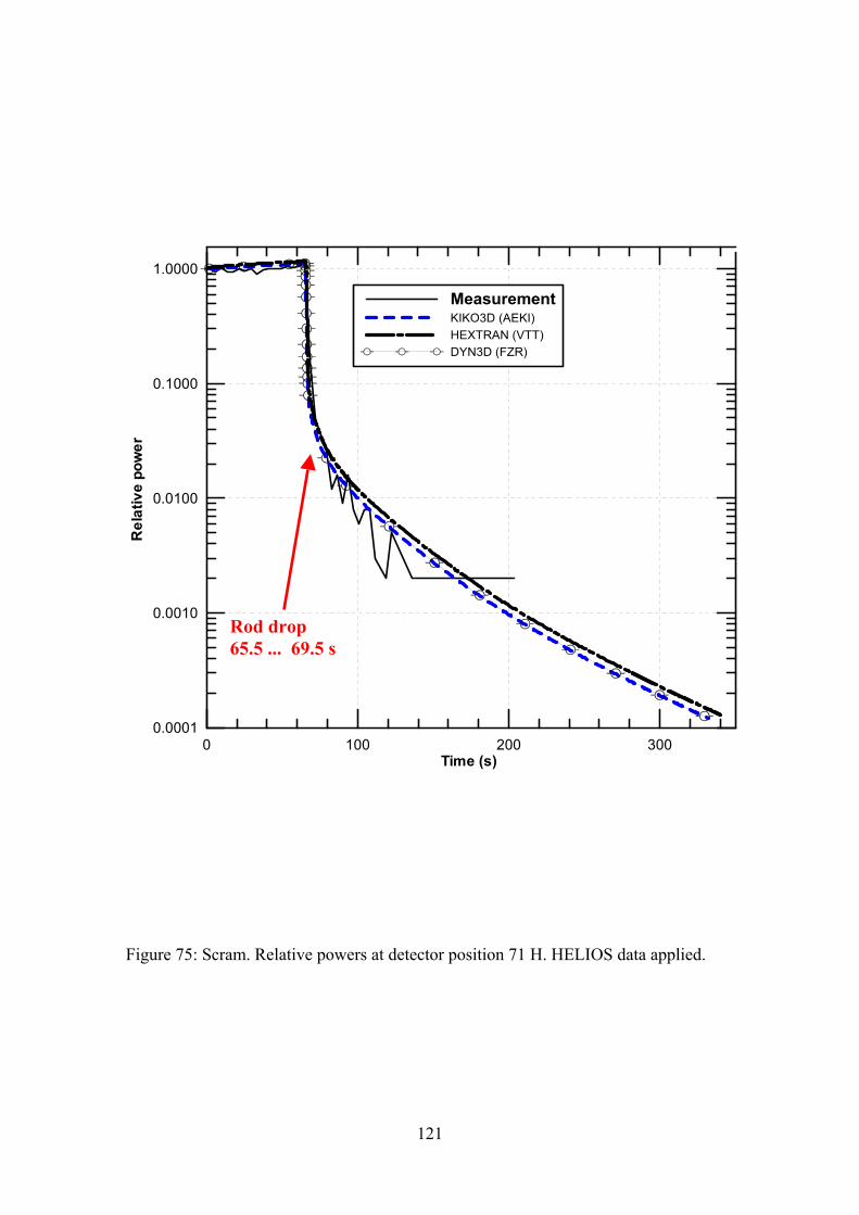
Rod drop 65.5 ... 69.5 s

0 100 200 300Time (s)

0.0001

0.0010

0.0100

0.1000

1.0000

Rel

ativ

e po

wer

MeasurementKIKO3D (AEKI)HEXTRAN (VTT)DYN3D (FZR)

Figure 75: Scram. Relative powers at detector position 71 H. HELIOS data applied.

121

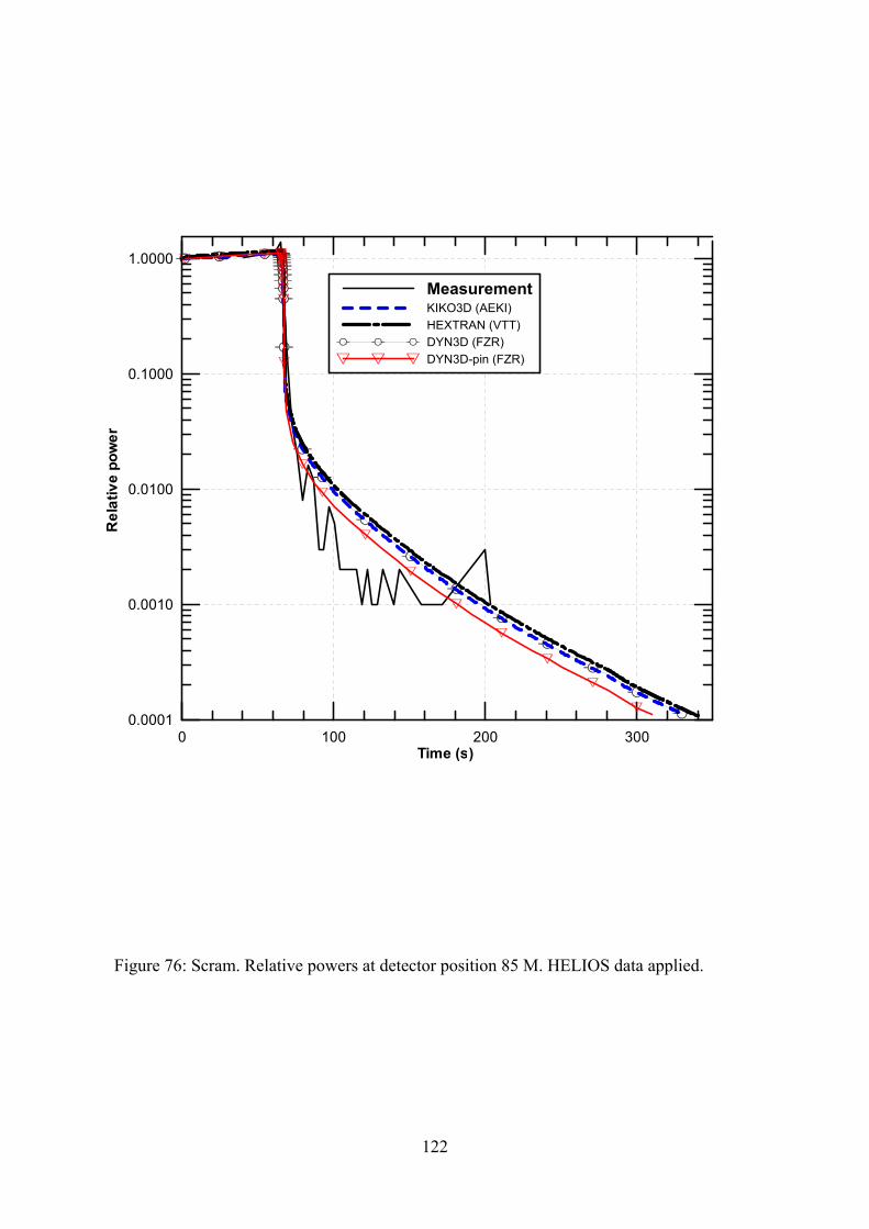
0 100 200 300Time (s)

0.0001

0.0010

0.0100

0.1000

1.0000

Rel

ativ

e po

wer

MeasurementKIKO3D (AEKI)HEXTRAN (VTT)DYN3D (FZR)DYN3D-pin (FZR)

Figure 76: Scram. Relative powers at detector position 85 M. HELIOS data applied.

122

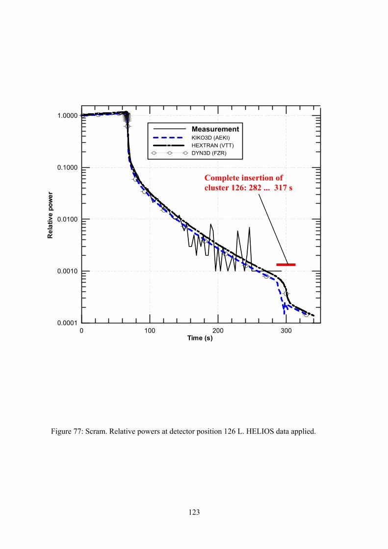
0 100 200 300Time (s)

0.0001

0.0010

0.0100

0.1000

1.0000

Rel

ativ

e po

wer

MeasurementKIKO3D (AEKI)HEXTRAN (VTT)DYN3D (FZR)

Complete insertion of cluster 126: 282 ... 317 s

Figure 77: Scram. Relative powers at detector position 126 L. HELIOS data applied.

123

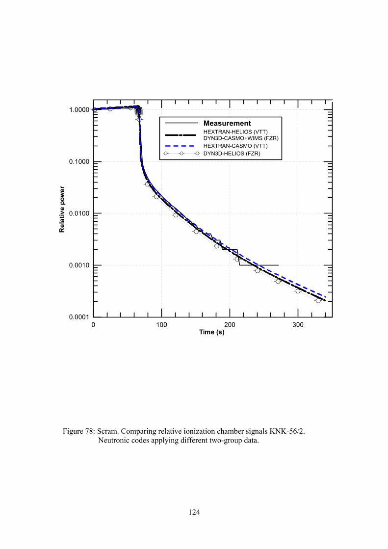
0 100 200 300Time (s)

0.0001

0.0010

0.0100

0.1000

1.0000

Rel

ativ

e po

wer

MeasurementHEXTRAN-HELIOS (VTT)DYN3D-CASMO+WIMS (FZR)HEXTRAN-CASMO (VTT)DYN3D-HELIOS (FZR)

Figure 78:

Scram. Comparing relative ionization chamber signals KNK-56/2.Neutronic codes applying different two-group data.

124