¶v &rqvxphu behavior study: preliminary evaluation … · behavior study: preliminary...
TRANSCRIPT
EPRI Project Manager B. Neenan
865-218-8133
3420 Hillview Avenue Palo Alto, CA 94304-1338 USA PO Box 10412 Palo Alto, CA 94303-0813 USA 800.313.3774 650.855.2121 [email protected]
www.epri.com May 13, 2013
Behavior Study: Preliminary Evaluation for
the Summer 2012

Acknowledgments The following organizations, under contract to the Electric Power Research Institute (EPRI), contributed to the preparation of this report:
Christensen Associates Energy Consulting
Daniel Hansen Marlies Hilbrink Dr. Richard Boisvert (Cornell)
EPRI Principal Investigator
Bernard Neenan, Technical Executive
This report describes research conducted by EPRI for FirstEnergy Corp

iii
Product Description
FirstEnergy designed a consumer behavior study (CBS) to inform the development of demand response programs that
demand and achieve other goals, such as reduced electricity usage at times when supply prices are high or system reliability is in jeopardy. The focal point was to quantify how residential customers respond to a monetary inducement (Peak Time Rebate (PTR)) to reduce load during pre-specified hours
In addition, the study evaluated the impacts of two response-enabling technologies, in-home displays (IHD) and programmable controllable thermostats (PCT), on customer response. Only customers identified as having central air conditioning were eligible to receive a PCT. The remaining customers without central air were eligible to receive an IHD.
Two novel aspects were included to resolve important ambiguities about how customers respond to PTR-type incentives. First, at the beginning of events (hot summer days) FirstEnergy sent a signal to PCTs for two of the treatment groups that raised thermostat setting three degrees. The third PCT treatment group was notified of the
make a PCT adjustment. Second, customers in the utility-initiated PCT treatment were further partitioned in terms of the event duration, four or six hours (event duration treatments). All treatment customers had the ability to opt-out of any PTR event, the utility-initiated ones by pushing an override button, but relative few elected to do so.
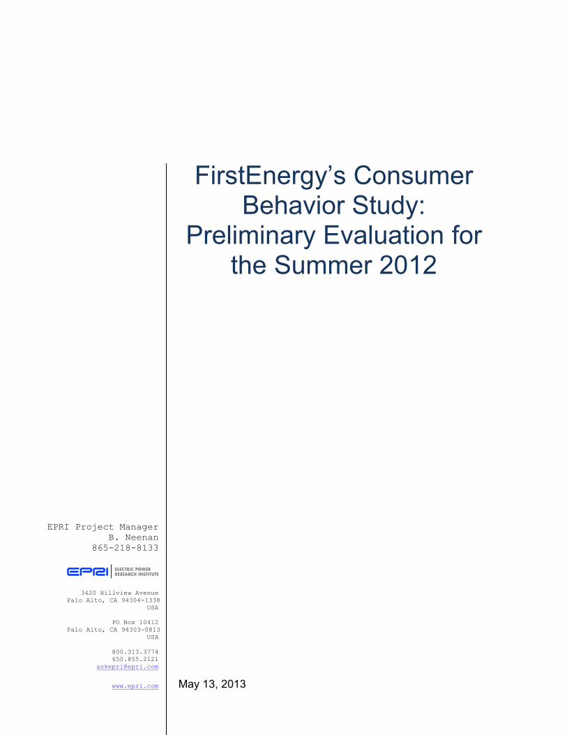
The figure below portrays the experimental design. Control groups were filled by random assignment. The treatment groups were populated through recruitment. Offers were extended to eligible customers, separately for the PCT and IHD experiments, until the desired number of subjects was achieved or the customer pool was exhausted. Customers electing to make PCT adjustments themselves were assigned to the four-hour treatments. Those that elected utility-initiated PCT adjustments were randomly assigned to the 4-hour or 6-hour event duration treatment. All customers in the combined IHD and PTR treatments were exposed to 4-hour events.
iv
Recruitment occurred in the fall of 2011 and winter of 2012, after which the technology was deployed. PTR events (15) were called from June 1 to August 31, 2012.
FirstEnergy commissioned EPRI to conduct a preliminary CBS analysis using hourly metered data for June-August 2012 from 976 customers in the pilot (control and treatment groups) and demographic and premise data from a survey administered in the fall 2012. EPRI conducted a series of analyses initially involving graphic depictions of the customer usage by treatment cell, and then by applying structured models, fixed effects and electricity demand, to the data to quantify the impacts, event percentage load reductions and price elasticity, respectively, of the treatments. PTR resulted in significant usage reduction during events (15 were called). The reduction was considerably lower, but still statistically significant, for the group of customers that managed the PCT themselves during events. The average hourly reduction was approximately the same for the 4-hour and 6-hour treatments. The group that received an IHD and were offered PTR payments exhibited a load reduction similar to that of the self-managed PCTs.
PTR Price & Event Duration
Treatments
Enabling Technology Treatments
$.40/kWh4 hour
6 hour
Control Rate A
B
C
PCT Self PCT Company
A 1-2 (250)
B2 (172)B1 (91)
C2 (170)
1 2
IHD
B3 (93)
A 3 (200)
3
A 1/2 drawn randomly from the population of survey respondents with AC
B1 and B2/C2 recruited randomly from the population of survey respondents with AC, given a choice of self-controlled or FirstEnergy-controlled PCT
B2/C2 were recruited to the PCT Company treatments and then randomly assigned to the 4-hour and 6-hour treatments
A3 drawn from the population without central AC, B3 recruited randomly from that population
976 Total

v
Table of Contents
Section 1: Introduction ......................................................... 1-1
Section 2: CBS Experimental Design .................................. 2-1 Introduction .......................................................................... 2-1 Baseline for Peak Time Rebate (PTR) ................................. 2-2 Day-Ahead Notification ........................................................ 2-3 CBS Experimental Design ................................................... 2-3 Customer Access to Information Regarding Their Usage .................................................................................. 2-5 Project Schedule and Timeline ............................................ 2-6 Customer Recruitment and Retention .................................. 2-6 Customer Survey Approach ................................................. 2-7
Section 3: Description of the Data ....................................... 3-1 Customer Electricity Usage Data ......................................... 3-1 Usage Patterns .................................................................... 3-3 Demographic Characterizations ........................................... 3-6 Enabling Technology Influences .......................................... 3-9
Section 4: Analytical Methodologies Employed ................. 4-1 Graphical Depictions of Average Electricity Usage .............. 4-2 Hourly and Daily Fixed Effects Models ................................ 4-8 Constant Elasticity of Substitution (CES) ........................... 4-10 Daily Elasticity Models ....................................................... 4-12
Section 5: Results of the Analysis ....................................... 5-1 Hourly and Daily Fixed Effects Regression Analysis ............ 5-1 Estimated Load Impacts Across Event Days ....................... 5-6 Constant Elasticity of Substitution (CES) Models ............... 5-10 Daily Elasticity of Demand Model ...................................... 5-11
Section 6: Summary and Conclusions ................................ 6-1 Background ......................................................................... 6-1 Findings .............................................................................. 6-3

vi
Appendix A: Validation of the Data .................................... A-1
Appendix B: The ANOVA Analyses .................................... B-1
Appendix C: Detailed Results for all Estimated Fixed Effects Models .................................................... C-1
Appendix D: Complete Results from the Estimated Economic Models .............................................. D-1
Appendix E: Sample Frame Customer Demographics ...... E-1

vii
List of Figures
Figure 2-1 Enabling Technology Treatments ............................. 2-4
Figure 2-2 CBS Enrollment Flowchart ....................................... 2-5
Figure 2-3 Company Schedule for Phase 1 ............................... 2-6
Figure 3-1 Cell-Level Average Non-Holiday Non-Event Weekday Load Profiles ........................................................ 3-5
Figure 3-2 Control Group Average kWh and THI, Non-Holiday Weekdays ............................................................... 3-5
Figure 4-1 Cell-Level Average Hot Non-Event Weekday Load Profiles ....................................................................... 4-3
Figure 4-2 Cell-Level Average Event Load Profiles ................... 4-4
Figure 4-3 Cell-Level Average June Event Load Profiles ........... 4-6
Figure 4-4 Cell-Level Average July 4th Week Event Load Profiles ................................................................................ 4-6
Figure 4-5 Cell-Level Average August Event Load Profiles ....... 4-7
Figure 5-1 Cell-Level Average Event Load Impacts ................... 5-5
Figure 5-2 PCT Customer-4 hr (B1) Average Load Reductions by Event ............................................................ 5-7
Figure 5-3 PCT Utility-4 hr (B2) Average Load Reductions by Event .............................................................................. 5-7
Figure 5-4 PCT Utility-6 hr (C2) Average Load Reductions by Event .............................................................................. 5-8
Figure 5-5 IHD -4 hr (B3) Average Load Reductions by Event ................................................................................... 5-8
Figure 6-1 Enabling Technology Treatments ............................. 6-3
Figure E-1 Home Size ............................................................... E-1
Figure E-2 Type of Home .......................................................... E-2
Figure E-3 Own or Rent............................................................. E-3
Figure E-4 Education Level ....................................................... E-4
Figure E-5 Income Level ........................................................... E-5


ix
List of Tables
Table 2-1 Implementation of Recruitment of Customers into Treatments .......................................................................... 2-7
Table 3-1 Number of Customers in Treatment/Control Cells ..... 3-2
Table 3-2 Central Air Conditioning amoung Survey Respondents ....................................................................... 3-2
Table 3-3 CBS Recruitment and Participation Shares ............... 3-2
Table 3-4 Cell-level Average Electricity Usage on Non-Event Days .......................................................................... 3-4
Table 3-5 Distribution of Home Size by Treatment/Participation........................................................ 3-7
Table 3-6 Distribution of Home Type by Treatment/Participation........................................................ 3-7
Table 3-7 Distribution of Education by Treatment/Participation........................................................ 3-8
Table 3-8 Distribution of Income by Treatment/Participation ...... 3-9
Table 3-9 Customer Overrides of Utility-Controlled PCTs during Events .................................................................... 3-10
Table 5-1 Event-Hour Load Impacts from Fixed-Effects Models ................................................................................. 5-3
Table 5-2 Event-Hour Percent Load Impacts from Fixed-Effects Models ..................................................................... 5-4
Table 5-3 Daily Load Impacts from Fixed-Effects Models .......... 5-5
Table 5-4 Second Stage Model of Load Responsess .............. 5-10
Table 5-5 Elasticities of Substitution from CES Models ........... 5-12
Table 5-6 Daily Demand Elasticities from CES Models ........... 5-13
x
Table A-1 Share of Zero and Missing Values by Month and Treatment ............................................................................ A-2
Table A-2 Customers Excluded from the Analysis ..................... A-3
Table B-1 PCT Results from ANOVA Model .............................. B-4
Table B-2 IHD Results from ANOVA Model ............................... B-5
Table B-3 Summary of Cell-Level Treatment Effects from ANOVA Model ..................................................................... B-5
Table B-4 Comparison of Estimated Event-Hour Usage Changes, ANOVA and Hourly Fixed Effects Models (kWh per hour) .................................................................... B-6
Table C-1 Fixed-Effects Results for PCT Customers- 4hr (B1) versus PCT Control (Hours 1 through 8) ..................... C-2
Table C-2 Fixed-Effects Results for PCT Customers- 4hr (B1) versus PCT Control (Hours 9 through 16) ................... C-4
Table C-3 Fixed-Effects Results for PCT Customers- 4hr (B1) versus PCT Control (Hours 17 through 24) ................. C-5
Table C-4 Fixed-Effects Results for PCT Utility-4hr (B2) versus PCT Control (Hours 1 through 8) ............................. C-6
Table C-5 Fixed-Effects Results for PCT Utility-4hr (B2) versus PCT Control (Hours 9 through 16) ........................... C-7
Table C-6 Fixed-Effects Results for PCT Utility-4hr (B2) versus PCT Control (Hours 17 through 24) ......................... C-8
Table C-7 Fixed-Effects Results for PCT Utility-6hr (C2) versus PCT Control (Hours 1 through 8) ............................. C-9
Table C-8 Fixed-Effects Results for PCT Utility-6hr (C2) versus PCT Control continued (Hours 9 through 16) ........ C-10
Table C-9 Fixed-Effects Results for PCT Utility-6hr (C2) versus PCT Control (Hours 17 through 24) ....................... C-11
Table C-10 Fixed-Effect Results for IHD-4hr (B3) versus IHD Control (Hours 1 through 8) ....................................... C-12
Table C-11 Fixed-Effect Results for IHD-4hr (B3) versus IHD Control (Hours 8 through 16) ..................................... C-13
Table C-12 Fixed-Effect Results for IHD-4hr (B3) versus IHD Control (Hours 17 through 24) ................................... C-14
Table C-13 Daily Fixed-Effects Results for ............................ C-15

xi
Table C-14 Fixed-Effects with Event-Specific Variables for PCT Customer-4hr (B1) versus PCT Control (Hours 15 through 18) ....................................................................... C-16
Table C-15 Fixed-Effects with Event-Specific Variables for PCT Utility -4hr (B2) versus PCT Control (Hours 15 through 18) ....................................................................... C-19
Table C-16 Fixed-Effects with Event-Specific Variables for PCT Utility 6hr (C2) versus PCT Control (Hours 14 through 19) ....................................................................... C-22
Table C-17 Fixed-Effects with Event- Specific Variables for IHD-4hr (B3) versus IHD Control (Hours 15 through 18) ... C-25
Table D-1 CES Model 1 Results for all Treatment Cells ........... D-1
Table D-2 CES Model 2 Results for all Treatment Cells ........... D-2
Table D-3 Demand Elasticity Results Log-Linear Models ...... D-3
Table D-4 Demand Elasticity Model 2 Results for all Treatment Cells .................................................................. D-4


1-1
Section 1: Introduction In March of 2009, FirstEnergy made a commitment to the Public Utilities Commission of Ohio (PUCO or Commission) to apply for Federal Smart Grid Investment Grant funds available through the American Recovery & Reinvestment Act of 2009. The application for funding under this grant was filed in October of the same year. The application was also filed with the Commission to approve recovery of the funds to match the grant. The PUCO issued its approval of the application in June of 2010.
As part of that order, the Commission encouraged the Company to work with the Department of Energy (DOE) to develop a Consumer Behavior Study. The Company worked closely with the Technical Advisory Group (TAG) assigned to the project by the DOE to develop the design of its Consumer Behavior Study. The study was approved in March of 2011, and the objectives of the study are:
To determine the extent to which the program, developed as part of the Consumer Behavior Study, is a cost effective way to achieve peak demand reduction in compliance with the requirements of Ohio Senate Bill 221;;
To increase customer knowledge of and response to peak-time rebate (PTR) prices, and to further expand demand response through additional opt-in pricing options;;
To determine local and stakeholder support by monitoring custome -time pricing programs;;
and duration periods;;
load shape for various duration periods, on the level of demand reduction, and on the magnitude and duration of rebound after a PTR event period;; and
To study the coincidence of the peak demand reduction with the
market value of the demand reduction.

Add licensed header here or delete for copyright reports.
1-2
The study addresses whether the peak demand reduction is larger for utility-controlled programmable thermostats relative to the peak demand reduction when customers themselves control the thermostat. The study is also designed to determine whether the duration of an event affects the amount of peak demand reduction achievable. If PTR events are called on consecutive days, the analysis is designed to identify customer fatigue in terms of the level of demand response when events are called on consecutive days.
The study also examines the extent to which customers who do not have central air conditioning can take advantage of information regarding their energy usage and day-ahead notification of PTR event days to reduce their usage and earn a rebate for energy usage reductions during events.
The CBS involves an ambitious research agenda, and this is one reason that the study was designed in two phases. This report contains the results of the first phase conducted in the summer of 2012. The other reason for implementing the CBS in two stages is to comply with the PUCO requirement that stipulates that FirstEnergy is to conduct a first phase, analyze the results, and then report them along with recommendations for the structure and scope of the second phase, which would increase the participating population to approximately 44,000 customers.
The remainder of this report is organized into five sections. In Section 2, we describe the experimental design used in the study. The discussion includes describing the target population, the functional specifications of the programmable controllable thermostats and in-home displays, the methods by which customers were assigned to treatment and control groups, the methods for customer recruitment and retention, and the administration and results of two customer surveys.
This discussion is followed in Section 3 by an analysis of the hourly load data for both control and treatment customers. Load data are used to estimate the treatment effects, and the analytical methods used to estimate the treatment effects are discussed in detail in Section 4. To assist in the empirical specification of the analytical models, we begin Section 4 with a discussion of a series of figures that illustrates average hourly customer usage on event and non-event days. These figures provide an indication of the magnitude of the treatment effects that we should expect from the formal statistical models. Thus, the graphical representations of the data help inform the methods that were used to establish the significance of measured treatment effects. We conclude Section 4 with discussions of the empirical specification of the analytical models used to estimate the various treatment effects.
In Section 5, we discuss in detail the empirical results, focusing primarily on the results from the hourly and daily fixed-effects regression models and the results from the economic demand models designed to estimate the own-price elasticity of demand for electricity and the elasticity of

1-3
substitution between peak and off-peak electricity usage. In this section, we focus on the important empirical results, but the complete details of the estimated models are reported in the several appendices.
In the final section, Section 6, we summarize the results and discuss the important implications for the design of the second phase of the CBS study.
Detailed data that describe the estimated models are provided in appendices.


2-1
Section 2: CBS Experimental Design Introduction
The CBS study was conducted in a specific geographic area served by
Smart Grid research projects conducted under the auspices of the DOE Smart Gird Modernization Initiative (SGMI). Focusing the study on a defined geographic region accommodated the installation of Advanced Metering Infrastructure (AMI) to provide the metering and communication system needed to implement the CBS design.
A 34-circuit area located in the Illuminating Company service territory east of the city of Cleveland, Ohio was chosen for the study. An initial population of 15,000 customers in a subset of the area received a qualifying survey that identified what appliances they have in their homes and premise characteristics and demographic information. Customers were selected to participate in the study based in part on their responses to this survey.
Study participants received a smart meter capable of two-way communication. In-home enabling technologies offered as an inducement for customer participation in a treatment group included a programmable controllable thermostat (PCT) that was offered to customers that were pre-qualified (through the survey) to participate by having central air conditioning (CAC). Customers that did not have central air were eligible to be offered an in-home display (IHD) that shows their instantaneous usage.
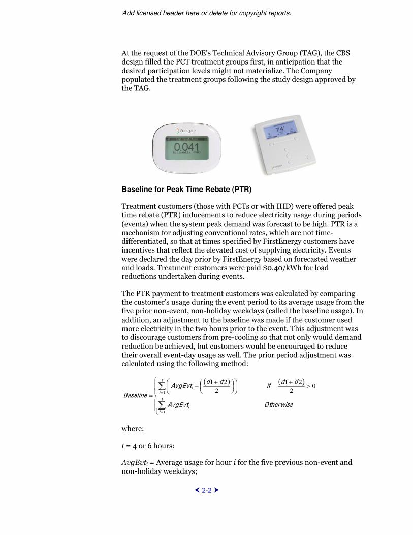
The PCT is an Energate thermostat (the device on the right below) that has two- cation network. The thermostat is capable of displaying messages and has a blue light that indicates that an event has been triggered. The PCT also has an override feature, which enables customers with PCTs under company-control to opt-out of an event. Upon installation, the contractor showed the customer how to program the PCT as well as how to override an event. In addition, they were provided with a call-in number to opt out of events in case they encountered difficulty with the PCT override feature.
The IHD (shown on the left below) provides real-time information
with the smart meter through a Zigbee communication network to display to a device, located within the premise, the custpoint in time. The device is also capable of displaying messages regarding events.
Add licensed header here or delete for copyright reports.
2-2
design filled the PCT treatment groups first, in anticipation that the desired participation levels might not materialize. The Company populated the treatment groups following the study design approved by the TAG.
Baseline for Peak Time Rebate (PTR)
Treatment customers (those with PCTs or with IHD) were offered peak time rebate (PTR) inducements to reduce electricity usage during periods (events) when the system peak demand was forecast to be high. PTR is a mechanism for adjusting conventional rates, which are not time-differentiated, so that at times specified by FirstEnergy customers have incentives that reflect the elevated cost of supplying electricity. Events were declared the day prior by FirstEnergy based on forecasted weather and loads. Treatment customers were paid $0.40/kWh for load reductions undertaken during events.
The PTR payment to treatment customers was calculated by comparing
five prior non-event, non-holiday weekdays (called the baseline usage). In addition, an adjustment to the baseline was made if the customer used more electricity in the two hours prior to the event. This adjustment was to discourage customers from pre-cooling so that not only would demand reduction be achieved, but customers would be encouraged to reduce their overall event-day usage as well. The prior period adjustment was calculated using the following method:
t
ii
t
ii
O therwiseAvgEvt
ddifddAvgEvtBaseline
1
10
221
221
where:
t = 4 or 6 hours:
AvgEvti = Average usage for hour i for the five previous non-event and non-holiday weekdays;;

2-3
d2 = Event day usage two hours prior to the event window minus the event window hour average of the previous five non-event, non-holiday weekdays;;
d1 = Event day usage one hour prior to the event window minus the -event non-holiday
weekdays;; and
The average of d2 and d1 is suadjusted baseline.
Day-Ahead Notification
Customers were notified on a day-ahead basis that an event would be in force the next day. Events were always declared for a pre-established event window, either four or six consecutive hours starting at a pre-
communication device to the PCT or IHD as well as through two other methods of the c -mail, and text message).
CBS Experimental Design
FirstEnergy employed the principles of a randomized control trial (RCT) design to isolate the effects of PTR monetary inducements and PCT and IHD technologies from other factors that influence household electricity demand. Control customers were selected randomly from the sampling frame, consistent with a RCT. However, for each treatment subjects were selected randomly as candidates from the sample frame and offered the opportunity to participate in that treatment. Those that accepted the offer to participate were enrolled in the pilot. Those that did not were removed from consideration in any other treatment.1
The study design called for testing the impacts of PCTs that control central air conditioners. Hence, eligible customers were sorted by those that had a central air conditioner and those that did not. The former were eligible to participate in the PCT treatments, and the latter in the IHD treatments. The result of this partition is that the study involved two separate technology treatment experiments;; one to test PCT effects and another to test IHD effects. In both cases, the technology was coupled with the PTR inducement to reduce event electricity usage. A separate
1 FirstEnergy employed the principles of a randomized control trial (RCT) design to isolate the effects of PTR monetary inducements and PCT and IHD technologies from other factors that influence household electricity demand. Control customers were selected randomly from the sampling frame, consistent with a RCT. However, for each treatment subjects were selected randomly as candidates from the sample frame and offered the opportunity to participate in that treatment. Those that accepted the offer to participate were enrolled in the pilot. Those that did not were removed from consideration in any other treatment.

Add licensed header here or delete for copyright reports.
2-4
control group, comprised of the customers that are eligible for the treatment, was drawn for each experiment.
Figure 2-1 portrays the CBS experimental design. The cells (elements of the design) are depicted as colored boxes labeled alphanumerically that correspond to control cells (A 1-2 and A3) and treatment cells (B1, B2, B3, and C2) that consist of a rate treatment (PTR payment of $0.40/kWh) for either a 4-hour or 6-hour event duration combined with an enabling technology treatment (PCT or IHD). The values in parentheses in the cells are the number of participants that were recruited (or randomly drawn, in the case of the control groups) into each cell. A consequence of this experimental design is that it was feasible to test directly for the effects of IHD versus the PCT, or to test for the effects of the IHD versus the length of the PTR event duration.
Figure 2-1 Enabling Technology Treatments
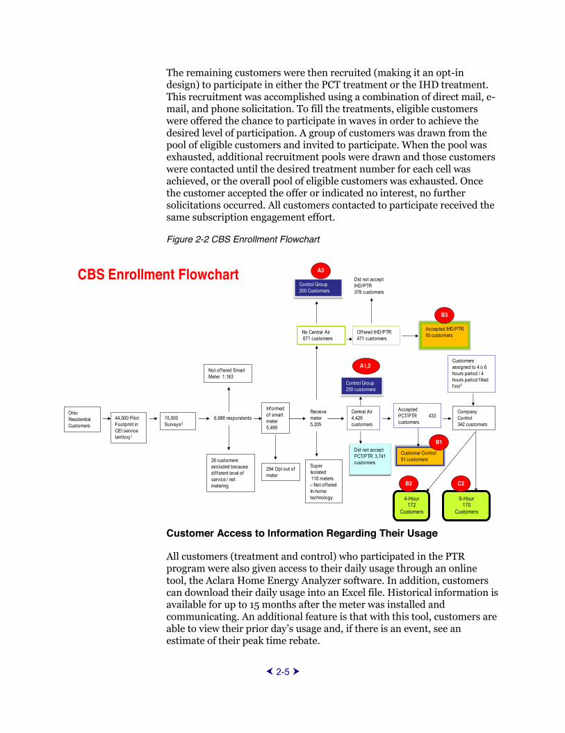
Figure 2-2 illustrates how customers that comprise the sampling frame were identified and how customers were recruited to participate as treatment subjects or controls. The CBS sampling frame was comprised of customers that responded to the pre-qualifying survey. There were 6,688 respondents to the survey (about 42% of those surveyed). Of that group, 26 were identified as having service levels that would not support the meter installation. The remaining 5,489 customers were offered the installation of a smart meter. These customers were then divided into those that had central air conditioning and those that did not. A control group was drawn from each group (250 customers for the PCT treatment group and 200 customers for the IHD group).
PTR Price & Event Duration
Treatments
Enabling Technology Treatments
$.40/kWh4 hour
6 hour
Control Rate A
B
C
PCT Self PCT Company
A 1-2 (250)
B2 (172)B1 (91)
C2 (170)
1 2
IHD
B3 (93)
A 3 (200)
3
A 1/2 drawn randomly from the population of survey respondents with AC
B1 and B2/C2 recruited randomly from the population of survey respondents with AC, given a choice of self-controlled or FirstEnergy-controlled PCT
B2/C2 were recruited to the PCT Company treatments and then randomly assigned to the 4-hour and 6-hour treatments
A3 drawn from the population without central AC, B3 recruited randomly from that population
976 Total
2-5
The remaining customers were then recruited (making it an opt-in design) to participate in either the PCT treatment or the IHD treatment. This recruitment was accomplished using a combination of direct mail, e-mail, and phone solicitation. To fill the treatments, eligible customers were offered the chance to participate in waves in order to achieve the desired level of participation. A group of customers was drawn from the pool of eligible customers and invited to participate. When the pool was exhausted, additional recruitment pools were drawn and those customers were contacted until the desired treatment number for each cell was achieved, or the overall pool of eligible customers was exhausted. Once the customer accepted the offer or indicated no interest, no further solicitations occurred. All customers contacted to participate received the same subscription engagement effort.
Figure 2-2 CBS Enrollment Flowchart
Customer Access to Information Regarding Their Usage
All customers (treatment and control) who participated in the PTR program were also given access to their daily usage through an online tool, the Aclara Home Energy Analyzer software. In addition, customers can download their daily usage into an Excel file. Historical information is available for up to 15 months after the meter was installed and communicating. An additional feature is that with this tool, customers are
estimate of their peak time rebate.
Ohio Residential Customers
44,000 Pilot Footprint in CEI service territory1
15,000 Surveys2
6,688 respondents
26 customers excluded because dif ferent level of service / net metering
Informed of smart meter 5,499
Not of fered Smart Meter 1,163
294 Opt out of meter
Receive meter 5,205
Super Isolated110 meters Not of fered
In-home technology
Control Group 200 Customers
No Central Air 671 customers
Central Air 4,429 customers
Offered IHD/PTR 471 customers
Accepted IHD/PTR 93 customers
Did not accept IHD/PTR 378 customers
Control Group 250 customers
Accepted PCT/PTR 433 customers
Did not accept PCT/PTR 3,741 customers
Customer Control 91 customers
Company Control 342 customers
CBS Enrollment Flowchart
Customers assigned to 4 o 6 hours period / 4 hours period f illed f irst3
4-Hour 172
Customers
6-Hour170
Customers
B3
A3
A1,2
B1
C2B2

Add licensed header here or delete for copyright reports.
2-6
Project Schedule and Timeline
AMI meters were installed in the spring of 2011 at 5,205 premises with the intent to collect a baseline of information during the summer of 2011. No information regarding the upcoming pricing program was provided to the customers at the time of installation.
After the summer of 2011, FirstEnergy began soliciting customers to participate in the program with the intent that the in-home technologies would be installed, sufficient testing completed, and data collection and billing processes would be in place so that the PTR program could commence on June 1, 2012. FE commissioned EPRI to conduct a preliminary analysis of the summer 2012 impacts in order to support a decision by the Public Utilities Commission of Ohio on whether Phase II, involving up to an additional 39,000 customers, would go forward.
Figure 2-activities.
Figure 2-3 Company Schedule for Phase 1
Customer Recruitment and Retention
Customers were recruited using a combination of direct mail, e-mail, and telephone marketing efforts. Table 2-1 below contains the percentages of customers from which the Company was able to get an affirmative accept, decline or not eligible response out of the total number that were sent the marketing materials. The Company sought to fill, but not overfill, treatment groups. Table 2-1 also indicates the levels of customer acceptance with each marketing campaign

2-7
Table 2-1 Implementation of Recruitment of Customers into Treatments
An attempt was made to contact all customers (except customers in the control groups) through direct mail, e-mail and outbound calling. The levels of customer retention were very high. Of the 533 customers who were subscribed to treatments initially, only seven had their devices removed prior to program inception. Two customers opted out during the program. One was dissatisfied with their thermostat and the other was moving to a different state.
Customer Survey Approach
The Company administered two surveys during Phase I. The pre-treatment survey was an appliance survey to prequalify customers for treatment. This survey also captured demographic and household information. The second survey, a post-treatment survey, was administered to program participants (treatment subjects) at the end of the program period in order to obtain their reactions and feelings toward the program. Customers who chose not to participate were also surveyed to get more information about why these customers did not want to participate in the program. Some information from this survey is used in Section 3 to characterize the sample, and will be used subsequently to fine-tune the marketing efforts for Phase II.2
2 The survey instruments are available upon request under a separate cover.


3-1
Section 3: Description of the Data In this section, we describe the hourly load data used in the analysis of treatment effects. Throughout the discussion, we focus on comparisons of average hourly usage levels and patterns for customers in the control and treatment groups, as well as on any differences in three important demographic characteristics-- the size and type of home, the level of education, and income.
Customer Electricity Usage Data
The study intended to collect hourly load data for approximately 5,200 premises who responded to the initial CBS survey and where a smart meter was installed. The electricity usage data are available for some customers beginning as early as June 2011.
The load data during the CBS study period (June 2012 through August 2012) are sufficiently reliable for use in the analyses. The study period database contains hourly usage values from June 1 through August 31, 2012 for the 976 customers that comprise the control and treatment subjects. Forty-two of these customers are excluded from the analysis because their usage data are compromised by missing or zero readings (Table 3-1).3 Therefore, the study period electricity usage data summarized in this report and used in the evaluations correspond to the remaining 934 customers.
Participants in the CBS were distributed among treatment and control cells. As explained above, the control groups were filled by random assignment. The treatment cells were filled using opt-in recruitment. Programmable controllable thermostats (PCTs) were only offered to customers with central air conditioning (CAC) in their homes. In-home displays (IHD) were offered to customers who did not have CAC. Customers with PCTs and who were offered a peak-time rebate (PTR) were given the choice between utility- and self-control of the PCT during event hours. The customers who elected to have FirstEnergy control their PCT were further divided (randomly) into groups with 4- and 6-hour event windows. The distributions of customers among treatment and control cells, as well as the distribution of customers removed from the database due to high shares of zero values for hourly usage, are contained in Table 3-1.
3A customer is excluded from the database if more than two percent of its non-holiday weekday hourly observations between June 1 and August 31, 2012 equal zero. See Appendix A for a list of the 42 customers excluded from the database using this criterion.
Add licensed header here or delete for copyright reports.
3-2
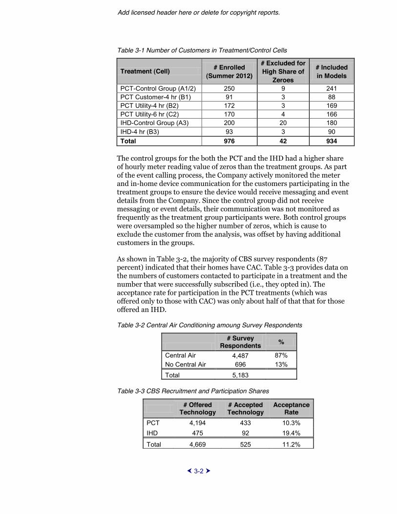
Table 3-1 Number of Customers in Treatment/Control Cells
Treatment (Cell) # Enrolled (Summer 2012)
# Excluded for High Share of
Zeroes
# Included in Models
PCT-Control Group (A1/2) 250 9 241 PCT Customer-4 hr (B1) 91 3 88 PCT Utility-4 hr (B2) 172 3 169 PCT Utility-6 hr (C2) 170 4 166 IHD-Control Group (A3) 200 20 180 IHD-4 hr (B3) 93 3 90 Total 976 42 934
The control groups for the both the PCT and the IHD had a higher share of hourly meter reading value of zeros than the treatment groups. As part of the event calling process, the Company actively monitored the meter and in-home device communication for the customers participating in the treatment groups to ensure the device would receive messaging and event details from the Company. Since the control group did not receive messaging or event details, their communication was not monitored as frequently as the treatment group participants were. Both control groups were oversampled so the higher number of zeros, which is cause to exclude the customer from the analysis, was offset by having additional customers in the groups.
As shown in Table 3-2, the majority of CBS survey respondents (87 percent) indicated that their homes have CAC. Table 3-3 provides data on the numbers of customers contacted to participate in a treatment and the number that were successfully subscribed (i.e., they opted in). The acceptance rate for participation in the PCT treatments (which was offered only to those with CAC) was only about half of that that for those offered an IHD.
Table 3-2 Central Air Conditioning amoung Survey Respondents
# Survey
Respondents %
Central Air 4,487 87% No Central Air 696 13% Total 5,183
Table 3-3 CBS Recruitment and Participation Shares
# Offered Technology
# Accepted Technology
Acceptance Rate
PCT 4,194 433 10.3% IHD 475 92 19.4%
Total 4,669 525 11.2%

3-3
As discussed in more detail below, customers with CAC have different average usage levels and patterns of use than do those who do not have CAC. Because of the differences in usage between customers with and without CAC, and the fact that all PCT customers have CAC and no IHD customers do, we are unable to make direct comparisons between the effectiveness of PCTs and IHDs. The design therefore does not randomize over customer circumstances, it in fact distinguishes them for the onset. This means that we can simplify the analysis somewhat by conducting separate analyses for the PCT treatment for each technology. However, comparing load impacts (the PCT effect) across the two experiments is not straightforward.
Usage Patterns
In the next series of tables and figures, we underscore differences in usage levels and patterns of usage between PCT and IHD customers, as well as differences among treatment and control groups. These latter comparisons may be affected by the fact that control-group customers were randomly selected while treatment customers volunteered (opted-in) to participate in a treatment group;; those that opted in to the program may be somewhat different from those included in the sample frame.
Table 3-4 contains summaries of average energy usage over different aggregations of hours for each treatment and control cell.4 Compared with IHD customers, PCT customers have higher average electricity usage in all periods, as well as higher ratios of peak to off-peak period usage. The customer-controlled PCT treatment group uses less electricity on average than do the other PCT groups, particularly during peak hours. The IHD customers who elected to participate have higher (about 11%) average usage than do those that comprise the IHD control group.
4 The average usage values are calculated from June 1 through August 31, 2012, excluding weekends, holidays, and event days.

Add licensed header here or delete for copyright reports.
3-4
Table 3-4 Cell-level Average Electricity Usage on Non-Event Days
Average Non-Holiday Non-Event Weekday kWh
During:
Cell All
Hours Peak Hours (1:00-7:00
PM) Off-peak
Hours P/O Ratio
PCT-Control Group (A1/2) 1.48 1.95 1.32 1.45 PCT Customer PCT Control - 4 hr. (B1) 1.35 1.76 1.21 1.42 PCT Utility- 4 hr. (B2) 1.41 1.86 1.26 1.45 PCT Utility- 6 hr. (C2) 1.45 1.88 1.30 1.42 IHD-Control Group (A3) 1.15 1.34 1.09 1.23 IHD - 4 hr. (B3) 1.28 1.44 1.22 1.18
Figure 3-1 contains an illustration of average weekday (excluding holidays) hourly usage patterns for the treatment and control groups.5 We see that customers in PCT treatment cells exhibit usage patterns that are noticeably different from customers in IHD treatment cells.
However, the graphics in Figure 3-1 suggest that usage patterns for the PCT control group are quite similar to usage patterns for the utility-controlled PCT treatment cells (B2 and C2), but the usage patterns during business hours for customer-controlled PCTs (cell B1) are lower than for customers in other PCT cells.6 The customers in the IHD control group (cell A3) exhibit an average usage pattern similar to that of the treatment cell (B3), although the average load profile for the control group is consistently lower than it is for the IHD treatment group.
Figure 3-2 illustrates the relationship for non-holiday weekdays between weather conditions and customer usage levels by plotting average hourly electricity usage for customers in the PCT and IHD control groups against the average hourly Temperature-Humidity Index (THI) during the six-hour event window. Solid data points represent event days and squares represent the PCT control group (A1|2).
5Vertical bars indicate the six-hour event window (1:00 p.m. - 7:00 p.m.). For ease of comparison, Figure 3-1 and subsequent load profile graphs include dashed lines indicating hourly Temperature-Humidity Index (THI) values averaged over dates corresponding to the load profiles displayed (measured on the secondary y-axis). This THI is based on data from nearby weather stations, and it is calculated as: THI = DB 0.55*(1-HUM)*(DB-58), where DB = Dry Bulb temperature (degrees Fahrenheit) and HUM = Relative Humidity (where 100% = 1). PJM Manual for Load Forecasting and Analysis;; PJM Manual 19, Revision 21;; effective October 1, 2012;; p.10.
6 Because of incomplete pre-treatment data, we cannot determine whether differences in the non-event day load profiles across treatment groups are due to self-selection effects (the customer-controlled participants were different from the utility-controlled participants) or treatment effects (the customer-controlled PCT participants engaged in conservation on non-event days causing their load profile to differ from that of the utility-controlled participants).

3-5
Figure 3-1 Cell-Level Average Non-Holiday Non-Event Weekday Load Profiles
Figure 3-2 Control Group Average kWh and THI, Non-Holiday Weekdays
0.00
0.50
1.00
1.50
2.00
2.50
3.00
3.50
4.00
4.50
1 3 5 7 9 11 13 15 17 19 21 23Hour
kWh
46
50
54
58
62
66
70
74
78
82
THI
Control-PCT (A1/2) Control-IHD (A3)PCT Customer-4hr (B1) PCT Utility-4hr (B2)IHD-4hr (B3) PCT Utility-6hr (C2)THI
0
0.5
1
1.5
2
2.5
3
3.5
4
50 55 60 65 70 75 80 85
Avg THI (1:00pm-7:00pm)
Avg
kW
h (1
:00p
m-7
:00p
m)
PCT-Control Group (A1/2) EventPCT-Control Group (A1/2) Non-EventIHD-Control Group (A3) EventIHD-Control Group (A3) Non-Event

Add licensed header here or delete for copyright reports.
3-6
Because of the presence of CAC, we would expect that PCT customers are more weather sensitive than IHD customers are, and this seems to be the case. On the days with the highest THI, average usage for PCT customers is nearly double that for IHD customers (approximately 3-4 kWh versus approximately 1.5-2 kWh, respectively).
Demographic Characterizations
As mentioned above, FirstEnergy administered a pre-study survey to collect data on appliance holdings and to sort customers for eligibility in the PCT treatments. These data help identify any differences in the socio-demographic characteristics among treatment and control customers. Note that only 42% of the surveyed customers returned a survey, and only a portion of those customers completed the demographic questions within the survey. Therefore, these responses may not be representative of the survey population or the total pool of survey respondents.
Tables 3-5 through 3-8 contain the distributions of responses to four demographic survey questions, distinguished by CBS treatment cell (and non-participation) and by the presence of CAC. There are some important differences in the demographic characteristics between customers with and without CAC. For example, CAC customers report larger average home sizes, are more likely to live in single-family homes, have higher education attainment, and report higher family income.7
Using the distributional data in tables 3-5 to 3-8, we are able to test for the similarity of demographic characteristics of control and treatment groups (more detailed data are provided in Appendix E). Based on these tests, there are no statistically significant differences in these demographic characteristics between the respective treatment and control groups. There are a couple of important exceptions. The distribution of home size for the utility-controlled, 6-hour PCT customers (cell C2) is different from the distribution for its control group, and the distribution of income for IHD treatment customers (cell B3) differs from that of its control group.
7 All of these differences are statistically significant at the 99 percent confidence level. Frequency distributions of each demographic characteristic for treatment and control groups (or CAC vs. Non-CAC) -squared test. This method tests for consistency between distributions, but where differences are significant;; it does not indicate how the distributions differ.

3-7
Table 3-5 Distribution of Home Size by Treatment/Participation
Home Size <1000 Sq Ft
1000-1499 Sq Ft
1500-1999 Sq Ft
2000-2999 Sq Ft
>=3000 Sq Ft know [blank]
Non-CAC IHD-Control Group (A3)
12% 19% 24% 22% 5% 12% 6%
IHD- 4 hr (B3) 9% 21% 24% 26% 13% 7% 0% No Treatment 11% 24% 22% 20% 9% 10% 5% CAC PCT-Control Group (A1/2)
0% 14% 24% 37% 19% 3% 2%
PCT Utility- 4 hr (B2)
2% 11% 20% 43% 19% 4% 2%
PCT Utility -6 hr (C2)
3% 9% 17% 47% 17% 4% 4%
PCT Customer- 4 hr (B1)
1% 7% 32% 33% 22% 2% 2%
No Treatment 3% 11% 22% 36% 21% 5% 2% Non-CAC Total 11% 22% 23% 22% 8% 10% 5% CAC Total 3% 11% 22% 37% 20% 5% 2% Grand Total 4% 13% 22% 35% 19% 5% 3%
Table 3-6 Distribution of Home Type by Treatment/Participation
Type of Home Single Family Home
Duplex or Two-Family
Home Condo-
minimum Mobile Home Other [blank]
Non-CAC IHD-Control Group (A3)
82% 1% 2% 13% 1% 2%
IHD- 4 hr (B3) 85% 1% 3% 8% 2% 0% No Treatment 80% 2% 5% 12% 0% 2% CAC PCT-Control Group (A1/2)
88% 0% 7% 3% 2% 0%
PCT Utility- 4 hr (B2)
84% 2% 8% 5% 1% 1%
PCT Utility- 6 hr (C2)
87% 1% 8% 3% 1% 1%
PCT Customer- 4 hr (B1)
92% 0% 4% 1% 2% 0%
No Treatment 90% 0% 5% 3% 1% 0% Non-CAC Total 81% 2% 4% 12% 0% 1% CAC Total 90% 0% 5% 3% 1% 0% Grand Total 89% 1% 5% 4% 1% 1%

Add licensed header here or delete for copyright reports.
3-8
Table 3-7 Distribution of Education by Treatment/Participation
Highest Level of Education
Element-ary
School or Less
Some High
School
Graduated High
School or Equivalent
Trade School
after High
School
Some College
Graduated College
Post-Graduate Degree
[blank]
Non-CAC IHD-Control Group (A3)
0% 6% 22% 6% 23% 24% 9% 8%
IHD-4 hr (B3) 0% 1% 15% 6% 30% 33% 9% 6% No Treatment 0% 5% 25% 6% 22% 21% 11% 11% CAC PCT-Control Group (A1/2)
0% 1% 12% 4% 18% 32% 22% 10%
PCT Utility- 4 hr (B2)
0% 2% 11% 4% 26% 30% 22% 6%
PCT Utility- 6 hr (C2)
0% 3% 13% 4% 25% 28% 22% 5%
PCT Customer- 4 hr (B1)
0% 1% 7% 4% 28% 34% 18% 8%
No Treatment 0% 1% 15% 4% 19% 33% 18% 9% Non-CAC Total 0% 5% 23% 6% 23% 24% 10% 9% CAC Total 0% 1% 14% 4% 20% 32% 19% 9% Grand Total 0% 2% 16% 4% 20% 31% 18% 9%

3-9
Table 3-8 Distribution of Income by Treatment/Participation
Enabling Technology Influences
When examining PTR event-hour load impacts, it is important to consider the fact that customers with utility-controlled PCTs (cells B2 and C2) are able to override the FirstEnergy-imposed thermostat adjustments on event days.
As seen in Table 3-9 below, on average eight percent of customers chose to override the FirstEnergy imposed increase of 3 degrees to their thermostats during events.8 Event-specific overrides rates ranged from 4% to 11%, but they do not appear to be systematically later in the summer (after 10 events), which would suggest fatigue. Because customer overrides of utility-controlled PCTs were enabled by the CBS design,
8Because of some irregularities in the override data such as duplicate records and timestamps that are inconsistent with event hours or override behavior (e.g. overrides recorded in the final minute of an event), we regard the values in Table 3-9 as an upper bound on the number of actual overrides that occurred during each event. That is, some of the reported overrides had time stamps indicating that a small (or zero) share of the event period was avoided by the overriding customer.
Income Category
<$15,000
>=$15,000 and
<$25,000
>=$25,000 and
<$35,000
>=$35,000 and
<$50,000
>=$50,000 and
<$75,000
>=$75,000 and
<$100,000
>=$100K and
<$150K
>=$150K and
<$200K >=$200K [blank]
Non-CAC IHD-Control Group (A3)
12% 13% 13% 14% 13% 7% 7% 2% 0% 19%
IHD- 4 hr (B3)
6% 9% 5% 21% 13% 11% 11% 2% 6% 16%
No Treatment
6% 18% 9% 13% 18% 9% 5% 1% 2% 19%
CAC PCT-Control Group (A1/2)
1% 6% 6% 8% 10% 16% 15% 8% 5% 24%
PCT Utility-4 hr (B2)
2% 8% 6% 11% 19% 11% 16% 6% 6% 15%
PCT Utility-6 hr (C2)
4% 6% 8% 12% 14% 11% 18% 5% 2% 20%
PCT Customer- 4 hr (B1)
3% 3% 9% 10% 18% 14% 11% 4% 4% 22%
No Treatment
3% 6% 7% 9% 14% 13% 13% 5% 5% 25%
Non-CAC Total
8% 15% 10% 14% 16% 9% 6% 1% 2% 19%
CAC Total 3% 6% 7% 9% 14% 13% 14% 5% 5% 25% Grand Total
3% 7% 7% 10% 14% 12% 13% 5% 4% 24%

Add licensed header here or delete for copyright reports.
3-10
electricity usage data for these instances are not excluded or otherwise treated differently in later analyses.
Table 3-9 Customer Overrides of Utility-Controlled PCTs during Events
PCT Utility-4 hr (B2) PCT Utility-6 hr (C2)
Event # Overrides
% Customers
Enrolled #
Overrides %
Customers Enrolled
1 19-Jun-12 11 6% 13 8% 2 20-Jun-12 17 10% 15 9% 3 21-Jun-12 11 6% 10 6% 4 29-Jun-12 15 9% 18 11% 5 2-Jul-12 14 8% 11 6% 6 3-Jul-12 13 8% 8 5% 7 5-Jul-12 7 4% 9 5% 8 6-Jul-12 17 10% 17 10% 9 16-Jul-12 14 8% 10 6%
10 17-Jul-12 11 6% 17 10% 11 23-Jul-12 19 11% 17 10% 12 26-Jul-12 17 10% 16 9% 13 3-Aug-12 18 10% 14 6% 14 16-Aug-12 13 8% 7 4% 15 24-Aug-12 17 10% 10 6% Event Average 14 8% 13 8%

4-1
Section 4: Analytical Methodologies Employed
We employ two basic analytical strategies to estimate the CBS treatment effects. The first category of analyses is statistical in nature, where established analytical methods are used to estimate the effects of the treatments and indicate the confidence level of the results. The second category relies on economic theory in addition to statistical methods to estimate behavioral-consistent models that impose the principle tenets of utility maximization for consumers.
To estimate the CBS treatment effects (changes in kWh during events and other times), we rely on analytical methods that are primarily statistical in nature. We first specify hourly customer fixed effects models. A separate model is estimated for each treatment cell relative to its control group. The coefficients from these models, estimated using data from the study period (June-August 2012), provide estimates of event-day treatment effects how electricity usage was affected by the PTR and enabling technology treatments. The estimates reveal differences between treatment and control group customer usage levels, controlling for differences in loads on non-event days, weather conditions, day-of-week effects, and customer-specific characteristics that do not vary over time (i.e., the customer fixed effects).9
Based on models that impose the economic tenets of consumer utility maximization, we also estimate two quite different price elasticities derived from separate electricity demand models. The elasticity of substitution between peak and off-peak electricity usage measures the percentage change in the ratio of average hourly peak usage to average hourly off-peak usage due to a one percent change in the inverse price ratio -- the ratio of the average hourly off-peak price to the average hourly peak price. These estimated elasticities of substitution are based on a constant elasticity of substitution (CES) demand model.
The second elasticity is a daily own-price elasticity of demand that measures the percentage change in average hourly daily use of electricity due to a one percent change in the average hourly daily price of electricity. 9 These load impacts are also estimated by methods of analysis of variance (ANOVA). This method of analysis, however, is most appropriate when the control group is representative of the treatment group. Customer self-selection into the treatment groups (via opt-in) produces customer groups that may not be comparable (in terms of pre-treatment loads) to the randomly selected control group. For this reason, the hourly fixed effects models are likely to provide superior estimates of the treatment effects. In Appendix B for completeness, we discuss the results from the ANOVA models and compare them with the results of the fixed effects models.
Add licensed header here or delete for copyright reports.
4-2
This own-price elasticity of demand is based on a log-linear demand model specification.10
By estimating these two elasticities, we can isolate the portion of the load impacts that are explained by the price incentives built into the PCT rate design. These price effects are an important component to the overall assessment of new rate programs that offer customers significant price incentives to alter load. Moreover, these elasticities are dimensionless measures of changes in usage, and, as such, they provide a common base of comparison for load impacts across studies.
Each of these methods is described in detail and the models are specified empirically in the topical sections that follow. Before specifying the empirical models, however, we first display graphically the data for average hourly customer usage on event and non-event days. Through a careful examination of these figures and graphs, we gain important insights into the magnitudes of treatment effects that we should expect to identify through the estimation of formal statistical and economic models. These insights, in turn, inform the methods and empirical specifications that are needed to estimate effectively treatment effects.
Graphical Depictions of Average Electricity Usage
Cell-level (treatments and controls) data for average hourly usage on hot non-event days - defined as days on which the maximum THI exceeds 78 - by CBS group are displayed in Figure 4-1. The figure displays only hot non-event days so that the usage profiles serve as an indicator of what event-day loads would have been in the absence of an event.11 The discussion that follows refers to treatments using the alphanumeric labels of Figure 3-1.
As evident in Figure 4-1, the hot day usage profile (average hourly electricity usage) for the PCT control group (A1|2) is very similar to those of the utility-controlled PCT treatment groups (cells B2 and C2). The customer-controlled PCT treatment group (cell B1), however, uses less electricity than does the PCT control group, particularly during the mid-day hours. The IHD treatment group uses more electricity than the IHD
10 Although the CES model and the log-linear demand model are based on somewhat restrictive assumptions. However, the equations needed to estimate the elasticities of substitution or the own price elasticities of demand can be modified to account for the effects of weather conditions and socio-economic characteristics of customers and premise characteristics on the willingness or ability of customers to change load in response to changes in electricity prices (e.g. D. Caves and L. Christensen. 1984.
-of-Use Electricity Pricing Journal of Econometrics, 26: 179-203).
11 Over half of the 15 event days had maximum THI greater than 80, however only two such non-event hot days are available. To broaden the sample of comparable non-event days without incorporating too many cooler days, a threshold of 78 was used. Accordingly, there are -event days;; 13 of 15 event days had maximum THI in excess of 78.

4-3
control group for the majority of the day. Both are considerable less than that of the AC groups during most of the hours of the day, and especially the during the peak hours.
While the demographic variables are not generally statistically different between the treatment and control groups, other unobservable characteristics could be different due to customer self-selection into the treatment groups. Given that PTR only provides incentives for customers to reduce usage on event days, we might expect the largest treatment effects to be limited to those days, such that the differences in usage between treatment and control group customers on non-event days are due to customer self-selection rather than treatment effects.12
These differences in usage across groups on event-like non-event days indicate the need to go beyond simple comparisons of usage levels in treatment and control groups using ANOVA models. Our fixed-effects models are needed because they account for usage differences on non-event days.
Figure 4-1 Cell-Level Average Hot Non-Event Weekday Load Profiles
12In theory, this hypothesis could be tested by comparing pre-treatment data (i.e., from 2011) across CBS groups. However, the pre-treatment data are not available for many of the CBS participants. Non-event day treatment effects could occur if customers alter their behavior on non-event days because of the PCT or IHD.
0.00
0.50
1.00
1.50
2.00
2.50
3.00
3.50
4.00
4.50
1 2 3 4 5 6 7 8 9 10 11 12 13 14 15 16 17 18 19 20 21 22 23 24Hour
kWh
46
50
54
58
62
66
70
74
78
82
THI
Control-PCT (A1/2) Control-IHD (A3)PCT Customer-4hr (B1) PCT Utility-4hr (B2)IHD-4hr (B3) PCT Utility-6hr (C2)THI

Add licensed header here or delete for copyright reports.
4-4
Figure 4-2 Cell-Level Average Event Load Profiles
Figure 4-2 illustrates average event-day usage profiles for each of the treatment and control groups. Several important observations are apparent from this figure, including:
Average electricity usage for the two utility-controlled PCT groups (B2 and C2) closely matched that of the PCT control group (A1|2) in the pre-event hours before usage declines substantially during the hours in the event window;;
The reduction in usage during PTR event hours for cells B2 and C2 (measured relative to the control group) declines as the event progresses. The decay in the response to the PTR incentive, which is the same for all event hours, is probably due to the fact that the PCT is set (by FirstEnergy) to be three degrees higher at the beginning of the event window. However, there are no further adjustments (by FirstEnergy) until the end of the event, when the thermostat (PCT) is reset to its start point, which may be at the setting in effect when the event was initiated. ;;
Customers in treatment groups B2 and C2 exhibit a substantial recovery or rebound effect;; usage during the hours just after the end of the event increases as the CAC system runs more than usual
0.00
0.50
1.00
1.50
2.00
2.50
3.00
3.50
4.00
4.50
1 2 3 4 5 6 7 8 9 10 11 12 13 14 15 16 17 18 19 20 21 22 23 24Hour
kWh
46
50
54
58
62
66
70
74
78
82
THI
Control-PCT (A1/2) Control-IHD (A3)PCT Customer-4hr (B1) PCT Utility-4hr (B2)IHD-4hr (B3) PCT Utility-6hr (C2)THI

4-5
-event set point;;
The customers who control their own PCT (cell B1) appear to reduce usage during pre-event hours as well as during event hours, but the average event period hourly reductions are much smaller than those for the utility-controlled PCT customers;;
There does not appear to be a rebound effect for customer-controlled PCT (B1) customers;; this effect may indicate that the apparent event usage reduction is not the result of an increase in the PCT temperature setting, or that the customers did not re-adjust the setting downward at the end of the event period;; and
IHD treatment customers (cell B3) appear to reduce usage during event hours. These reductions are evident by comparing the usage profiles for IHD treatment and control groups on event and non-event days (Figures 4-1 and 4-2). The reductions in usage appear to be considerably smaller than those for the utility-controlled and self-controlled PCT customers.
Figures 4-3 through 4-6 contain graphs of average event-day usage for each month in which PTR events were called. July events (Figures 4-4 and 4-5) are divided into two groups because the first four events of the month were called during the week that included the Fourth of July holiday. Separating these events from the others may isolate any effects of the holiday on customer behavior.
Our interpretations of the figures led to the following observations:
The magnitude of the load response by utility-controlled PCT customers is affected by weather conditions. The largest load reductions are in June and in late July when the weather was the hottest;;
It was considerably cooler during the August event days, which appears to have contributed to the reduced level of event response;;
While usage was lower during the week of the Fourth of July, it was also cooler than it was during other July event days, which makes it difficult to determine which effect caused the reduction in overall usage (the PCT price inducement or the facts that people were away from home and the thermostat setting was higher than usual for a weekday;; and
There may be a reduction in demand response by IHD treatment customers (cell B3) over the course of the summer. There is a more pronounced notch in usage during event hours in June than in the later months.

Add licensed header here or delete for copyright reports.
4-6
Figure 4-3 Cell-Level Average June Event Load Profiles
Figure 4-4 Cell-Level Average July 4th Week Event Load Profiles
0.00
0.50
1.00
1.50
2.00
2.50
3.00
3.50
4.00
4.50
1 2 3 4 5 6 7 8 9 10 11 12 13 14 15 16 17 18 19 20 21 22 23 24Hour
kWh
46
50
54
58
62
66
70
74
78
82
THI
Control-PCT (A1/2) Control-IHD (A3)PCT Customer-4hr (B1) PCT Utility-4hr (B2)IHD-4hr (B3) PCT Utility-6hr (C2)THI
0.00
0.50
1.00
1.50
2.00
2.50
3.00
3.50
4.00
4.50
1 2 3 4 5 6 7 8 9 10 11 12 13 14 15 16 17 18 19 20 21 22 23 24Hour
kWh
46
50
54
58
62
66
70
74
78
82
THI
Control-PCT (A1/2) Control-IHD (A3)PCT Customer-4hr (B1) PCT Utility-4hr (B2)IHD-4hr (B3) PCT Utility-6hr (C2)THI

4-7
Figure 4-5 Cell-Level Average Week of July 4 Event Load Profiles
Figure 4-5 Cell-Level Average August Event Load Profiles
0.00
0.50
1.00
1.50
2.00
2.50
3.00
3.50
4.00
4.50
1 2 3 4 5 6 7 8 9 10 11 12 13 14 15 16 17 18 19 20 21 22 23 24Hour
kWh
46
50
54
58
62
66
70
74
78
82
THI
Control-PCT (A1/2) Control-IHD (A3)PCT Customer-4hr (B1) PCT Utility-4hr (B2)IHD-4hr (B3) PCT Utility-6hr (C2)THI
0.00
0.50
1.00
1.50
2.00
2.50
3.00
3.50
4.00
4.50
1 2 3 4 5 6 7 8 9 10 11 12 13 14 15 16 17 18 19 20 21 22 23 24Hour
kWh
46
50
54
58
62
66
70
74
78
82
THI
Control-PCT (A1/2) Control-IHD (A3)PCT Customer-4hr (B1) PCT Utility-4hr (B2)IHD-4hr (B3) PCT Utility-6hr (C2)THI

Add licensed header here or delete for copyright reports.
4-8
Examination of average customer load profiles across treatment groups and types of days provides guidance for the formal statistical analyses. First, we expect to estimate substantial load impacts for the utility-controlled PCT treatment groups (cells B2 and C2). The post-event rebound effect also appears to be quite pronounced. We expect lower event-hour usage reductions for the customer-controlled PCT and even lower IHD treatment groups. Finally, differences in non-event day usage between treatment and control groups suggest the need to incorporate a differences-in-differences component into the statistical models. That is, the event-day load impacts will be based on the difference in usage between treatment and control groups on event days minus the difference in usage between those groups on non-event days (controlling for other factors such as weather and type of day
Hourly and Daily Fixed Effects Models
Graphic comparisons suggest that there are differences among the groups in event-day electricity use. However, establishing the level and significance (or lack thereof) of differences requires application of formal modeling methods.
Hourly fixed effects models are estimated in order to develop event-day load impacts for customers in each of the treatment cells. The experiment produces panel data- observations on electricity usage (kWh) over several customers (over 950) over an extended period (three months). A fixed effects formulation recognizes that there may be differences among subjects that do not vary over time and are not observed or measured. This challenges estimation of effects because the standard statistical formulation confounds time-vary and time-constant effects. A fixed effect formulation accommodates difference among customers structurally so that the treatment effect can estimated precisely and credible.13
A separate fixed effect model is estimated for each treatment cell and hour of the day (hour ending 1 through 24). Each model imposes a pair-wise combination of treatment and control customer group (i.e., A1|2 and B1, A1|2 and B2, A3 and B3, and A1|2 and C2) to identify changes in electricity usage during each hour of the event days.
To estimate this structure, it was necessary to estimate 96 different models (4 pair-wise combinations x 24 hours), and each model includes an indicator variable that equals one for treatment customers on event days only (among other variables). The estimated coefficient on this term in each model measures the average PTR effect on electricity usage for the treatment customers (as compared with control group customers) for each hour of an event day.
13 A formal explanation of the model specification and its justification and the mechanics of the estimation process are provided in: Wooldridge, J. 2010. Econometric Analysis of Cross Section and Panel Data. MIT Press, Cambridge, MA.

4-9
Each hourly fixed effects regression model is specified as follows:
where:
Qc,t represents the hour usage for customer c on non-holiday weekday t;; is the constant term;; The (subscripted to correspond to events (Evt), treatments (Trt), heat index (THI), moving average heat index (THIMA) and day type (DT), and combinations thereof, are estimated parameters;; Eventt is an indicator variable that equals one if day t is an event day, and zero otherwise;; Treatc is an indicator variable that equals one if customer c is in the treatment (i.e. not control) group, and zero otherwise;; THIt is the temperature-humidity index for the model hour on current day t;; THIMAt is the 24-hour moving average temperature-humidity index for the 24 hours prior to the model-hour on day t;; DTypei,t is a series of dummy variables for each day of the week that equal one for the specific day of the week, and zero otherwise;; vc is the fixed effect for customer c14 and ect is the error term.15
conditions (represented by current-hour THI and a 24-hour moving average), type of day, and event day. These effects are allowed to differ among customers in treatment and control groups through the inclusion of interaction terms created by multiplying each explanatory variable by an indicator variable for being in a particular treatment group (e.g., THIt x Treatc). The Eventt variable accounts for otherwise unexplained differences in usage on event-days between customers in treatment and control groups (e.g., if the included weather variables are not able to account fully for the event-day conditions). Our primary interest is the coefficient on the 14 Although these models are estimated by a fixed effects estimator in STATA, the procedure is equivalent to ordinary least squares when a dummy, or indicator variable is included for each customer. 15 We account for first-order serial correlation using the method contained in: Baltagi, B.
ata regressions with AR(1) Econometric Theory 15: 814-823. This method is used in the daily models
as well.
tccci
tTrtDT
i
it
DTict
TrtTHIMA
tTHIMA
ctTrtTHI
tTHI
ctTrtEvt
tEvt
tc
evTreatDType
DTypeTreatTHIMA
THIMATreatTHI
THITreatEventEventQ
,
5
2
_
5
2
_
_
_,
)(
)(
)(
)(

Add licensed header here or delete for copyright reports.
4-10
interaction term between Eventt and Treatc ( Evt_Trt) which represents the estimated average PTR event-day treatment effect for that hour expressed in kWh. In summary, the model recognizes several potential differences between customers in control and treatment groups. Usage can differ in several ways:
Average usage across all hours, through the customer-specific fixed effects;;
Weather sensitivity, through the interaction of the weather variables with the treatment indicator variable;;
Usage patterns across different types of days, through the interaction between type of day indicator variables with the treatment indicator variables;; and
Changes in event-day usage through the interaction of the event-day indicator variables with the treatment indicator variables.
When taken together, these modeling components comprise the differences-in-differences structure of the fixed effects model that improves upon methods (such as ANOVA) that estimate treatment effects through a simple comparison of usage between treatment and control groups on event days. As discussed above, the examination of graphs in Figures 4-1 through 4-5 compels moving beyond simpler ANOVA models to estimate load impacts.
To test whether there is a net conservation effect during event days, we also estimate daily models similar to hour-specific models. These models are identical to the specification of the hourly models presented above, except that the dependent variable is the average usage across all hours of the day, and the THI variables are specified as daily average values for the current and preceding days. In these models, the Evt_Trt coefficient is an estimate of the average hourly change in usage for the entire event day.
Constant Elasticity of Substitution (CES) To characterize how customers shift loads among hours in response to price changes, we estimate electricity demand in the form of a Constant Elasticity of Substitution (CES) model. This model characterizes load-shifting behavior through the elasticity of substitution.16 As with the hourly and daily fixed effects models described earlier, a separate model is estimated for each treatment group. Data for customers in its control group are included in the model as well, along with a series of variables that allow for differences in weather sensitivity between groups.
16 -peak electricity use is defined as the percentage change in the ratio of peak to off-peak electricity use caused by a 1 percent change in the ratio of off-peak to peak electricity prices.

4-11
The CES regression model is as follows:17
tctEvt
cOP
tP
tTr tTHI
OPt
Pt
THIPt
OPt
OPct
Pct
evEventTreatTHITHI
THITHIPPkWhkWh
)(
)()/ln()/ln(_
,,
where: kWhPt,c is the usage for customer c on day t during the peak hours, which is 2:00 to 6:00 p.m. for 4-hour utility-controlled PCT customers, and 1:00 to 7:00 p.m. for the 6-hour event treatment;; kWhOPt,c is the usage for customer c on day t during the off-peak hours;; PPt is the average electricity price ($/kWh) during the peak hours of day t;; POPt is the average electricity price ($/kWh) during the off-peak hours of day t18 The Eventt is an indicator variable that equals one if day t is an event day and zero otherwise;; THIPt equals average hourly THI during the peak hours of day t;; THIOPt equals average hourly THI during the off-peak hours of day t;; vc is the customer-specific fixed effect;; and et is the error term.
In this analysis, the term peak period is synonymous with event hours. That is, the model is designed to estimate the extent to which customers shift load from event to non-event hours during PTR event days. In the absence of the PTR incentive, the retail price is constant during the day. For participants on non-event days, and for nonparticipants on all days, the log inverse price ratio (ln(POP
t/PPt)) is equal to zero. Because the control
group customers are not exposed to any PTR event days (and hence their price never varies), they do not contribute directly to the estimation of the
control customers ( subscript c) in the model helps control for non-price-related changes in use associated with event-day conditions (superscrriptEvt) as well as for day-specific changes in use that affect everyone (et The Eventt variable is included in order to control for differences in event-day usage that are not explained by price or weather conditions. This variable is applied to both treatment and control group customers, and it 17 As suggested above, this model is consistent with the theory of consumer utility maximization. Although not evident in this empirical specification, the model can be modified to so that the elasticity of substitution can account for the effects of weather, customer or premise characteristics that may modify preferences (Caves and Christensen. 1984. op. cit., p. 186). 18 The non-event price is equal to $0.093248 = $0.02951 + $0.001747 + $0.061991. The peak price on event days is equal to $0.493248 = $0.40 + $0.093248 for PTR treatment customers.
Add licensed header here or delete for copyright reports.
4-12
ensures that represents the event-day treatment effect for PTR customers.
Daily Elasticity Models
In addition to the CES model, we estimate a daily own-price elasticity. This model measures how customers change their overall event-day usage in response to PTR incentives. The model is specified in log-linear form:
tctEvt
cAvg
tTr tTHI
Avgt
THIAvgtd
Avgct
evEventTreatTHI
THIPkWh
)(
)ln()ln(_
,
Where:
The terms are as defined above.
In this model, the usage, price, and THI variables are averaged across the hours of the day. The parameter d is the daily (own-price) elasticity of demand for electricity.19
Once estimated, the CES models and daily demand models can be used to simulate changes in event-day usage for treatment customers. That is, the CES model simulates the change in the ratio of event (or peak) to non-event hour usage, while the daily model simulates the change in the overall usage level.
Some caution, however, should be exercised extending the interpretation of estimates of the elasticities of substitution for this particular CBS program design to different price levels. We expect that the impact attributable the utility-controlled PCT customers is largely due to the effects of increasing the PCT temperature set point. Changing the PTR incentive level (e.g., from 40 cents/kWh to 80 cents/kWh) is not going to change the amount of load reduction that is obtained from increasing the PCT set point by three degrees. However, the higher incentive level could influence override behavior it declines. Moreover, a higher incentive could affect the behavior of customers who have customer-controlled PCTs, they might make adjustments of more than 3 degrees. Additionally, it might cause both to seek out other ways to reduce electricity and be paid for doing so. . Despite these precautions, elasticities of substitutions are useful in presenting a normalized measure of the amount of demand response that is forthcoming from this particular CBS program design.
19 Methods from Baltagi and Wu (1999) are used to control for first-order serial correlation in estimating the CES models and the models for daily own price elasticities of demand.

5-1
Section 5: Results of the Analysis In this section, we discuss in detail the empirical results derived from estimating the models described in Section 4. We begin with a discussion of results from the estimated fixed effects regression models designed to identify changes in electricity usage on PTR event days. We then move on to a discussion of results from the two demand models that are used to estimate elasticities of substitution and own-price elasticities of demand. Throughout, we report details of empirical results needed to understand the nature of the load response. For transparency in interpretation, it is often convenient to present some results graphically. Full details of the estimated equations are reported in Appendix B.
Hourly and Daily Fixed Effects Regression Analysis
As described in Section 4, separate models are estimated for each treatment group and its associated control group. Table 5-1 contains the estimated Evt_Trt coefficients that are measures of the changes in electricity usage on PTR event days for each treatment cell, expressed as kWh per customer. Estimates of these types of changes are provided for each hour of event days, averaged across all PTR events. The statistical significance of the coefficients (relative to a null hypothesis that the coefficient is zero) i -for the 99-percent level. Negative coefficients are interpreted as reductions in usage relative to what customers would have used in the absence of the PTR event (the reference load). In Table 5-2, we display the estimates as a percentage of the reference load,20 and in Figure 5-1, we illustrate the hourly load impacts for each treatment group.
As seen in Table 5-1, there is very little to no change in electricity usage during the pre-event hours for most treatments (the shaded boxes in the figures are the event hours). The exception is for customer-controlled PCT customers (cell B1), for which usage is lower during the pre-event hours of 8:00 a.m. through 2:00 p.m. It appears that when these customers respond to the PTR incentives, they do so by making modifications to their energy usage, perhaps by setting the PCT temperature higher before they leave for work or other out-of-home activity.
Changes in event-hour usage are uniformly statistically significant, but the magnitudes differ across treatment cells (Table 5-1). The utility-controlled PCT groups (cells B2 and C2), for example, show similar reductions in averages hourly usage of 0.85 and 0.77 kWh (Table 5-1) ,
20 Reference loads are calculated by adding the estimated load changes to the observed loads averaged across event days.

Add licensed header here or delete for copyright reports.
5-2
respectively, which is 30 and 28 percent of the reference loads, respectively (Table 5-2). In both cases, the magnitude of the reduction in usage is much higher at the beginning of the event window than it is at the end of it (declines by 50% or more). This is consistent with how the PCT is adjusted by the Company: it is increased by three degrees at the beginning of the event window and decreased by three degrees at the end.
The reductions in event-hour usage for the customers in the customer-controlled PCT and IHD treatments were substantially smaller. The customers in the customer-controlled PCT treatment group (cell B1) reduced usage by an average of 0.22 kWh (8 percent) during the event hours, while the customers in the IHD treatment group (cell B3) reduced usage by an average of 0.18 kWh (11 percent) during the event hours.
During the post-event hours, the rebound effect for utility-controlled PCT customers is substantial (both 4- and 6-hour events). Statistically significant increases in usage persist through to the end of the day (Table 5-1). By midnight, the total post-event usage increase was estimated to be 2.4 kWh for the customers with the 4-hour event window, which represents 71 percent of the total reduction in event-period usage). For the customers with the 6-hour event window, the rebound is 2.5 kWh, 54 percent of the total reduction in event-period usage.21 The size of the snap back emphasizes the need to consider how long and when events are called, or to take measures to bring loads back on in stages.
Neither customers in the customer-controlled PCT nor those in the IHD treatment groups experienced statistically significant increases in usage during the post-event hours, with the exception of the hour 10:00-11:00 p.m. for Group B3. This result may indicate that neither group achieved their reductions in event-hour usage by reducing the use of air conditioning, or that they adjusted the thermostat set point by less than the three degrees as in the case of the utility-controlled PCTs. If this were true, there would be little need to catch up (rebound) during in the post-event hours.
Through an examination of the daily fixed effects models we can identify estimates of changes in total load on event days, expressed in kWh per hour. As is seen in Table 5-3, three of the four treatment groups experienced statistically significant reductions in event-day usage. The largest of these conservation effects was estimated for customers in the 6-hour utility-controlled PCT treatment group (cell C2) who reduced event-day usage by 3 percent, or 0.06 kWh per hour. The usage reduction for customers in the 4-hour utility-controlled PCT treatment group was estimated with similar precision (a standard error of 0.016 versus 0.017
21 The fact that customers with the 6-hour event window have two more event hours and one fewer post-event hour than customers with the 4-hour event window clearly affects the results of these share calculations.

5-3
for the 6-hour customers), but the conservation effect was not quite large enough to be statistically significantly different from zero.
Table 5-1 Event-Hour Load Impacts from Fixed-Effects Models
Control Group versus:
Hour PCT
Customer-4 hr (B1)
PCT Utility-4 hr (B2)
PCT Utility-6 hr (C2)
IHD-4 hr (B3)
1 0.100++ 0.026 0.05 0.026 2 0.031 0.02 0.049+ -0.008 3 0.021 0.029 0.039+ -0.008 4 0.025 0.032 0.034+ -0.004 5 0.011 0.012 -0.002 -0.011 6 0.028 -0.002 0.026 -0.038 7 0.016 -0.002 0.031 0.023 8 -0.053 0.003 0.036 0.032 9 -0.076+ -0.004 -0.034 -0.059
10 -0.084+ 0.031 0.006 0.011 11 -0.126++ -0.018 -0.005 0.022 12 -0.133++ -0.011 0.086+ 0.047 13 -0.115+ 0.025 0.087+ 0.046 14 -0.110+ 0.099+ -1.077++ -0.034 15 -0.173++ -1.034++ -1.066++ -0.164++ 16 -0.195++ -0.995++ -0.898++ -0.163++ 17 -0.263++ -0.793++ -0.687++ -0.216++ 18 -0.261++ -0.556++ -0.456++ -0.194++ 19 -0.043 0.687++ -0.430++ 0.014 20 0.046 0.636++ 0.927++ -0.002 21 0.104 0.481++ 0.836++ -0.005 22 0.072 0.283++ 0.460++ 0.068 23 0.023 0.157++ 0.171++ 0.109++ 24 0.068 0.145++ 0.101++ 0.016
Event Average -0.223 -0.845 -0.769 -0.184
++ p<0.01, + p<0.05
For the customers in the customer-controlled PCT and the IHD treatment groups, the empirical results show statistically significant conservation effects of 2.o and 2.3 percent, respectively. The absence of a post-event rebound effect for these treatment groups made their overall conservation effect similar to those of the customers in the utility-controlled PCT treatment groups, despite the fact that their reductions in event-hour usage were much smaller in magnitude.

Add licensed header here or delete for copyright reports.
5-4
Table 5-2 Event-Hour Percent Load Impacts from Fixed-Effects Models
Control Group versus:
Hour PCT
Customer-4 hr (B1)
PCT Utility-4 hr (B2)
PCT Utility-6 hr (C2)
IHD-4 hr (B3)
1 7% 2% 3% 2% 2 2% 2% 4% -1% 3 2% 3% 4% -1% 4 3% 3% 3% 0% 5 1% 1% 0% -1% 6 3% 0% 2% -3% 7 1% 0% 2% 2% 8 -4% 0% 2% 2% 9 -5% 0% -2% -4%
10 -5% 2% 0% 1% 11 -7% -1% 0% 2% 12 -7% -1% 4% 3% 13 -5% 1% 4% 3% 14 -5% 4% -44% -2% 15 -7% -40% -41% -10% 16 -7% -36% -31% -10% 17 -9% -26% -22% -12% 18 -8% -17% -14% -10% 19 -1% 22% -13% 1% 20 2% 22% 31% 0% 21 4% 18% 30% 0% 22 3% 10% 17% 4% 23 1% 7% 7% 6% 24 3% 8% 5% 1%
Event Average -8% -30% -28% -11%
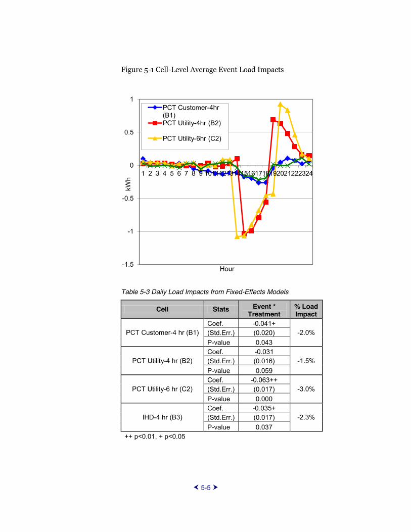
5-5
Figure 5-1 Cell-Level Average Event Load Impacts
Table 5-3 Daily Load Impacts from Fixed-Effects Models
Cell Stats Event * Treatment
% Load Impact
PCT Customer-4 hr (B1) Coef. -0.041+
-2.0% (Std.Err.) (0.020) P-value 0.043
PCT Utility-4 hr (B2) Coef. -0.031
-1.5% (Std.Err.) (0.016) P-value 0.059
PCT Utility-6 hr (C2) Coef. -0.063++
-3.0% (Std.Err.) (0.017) P-value 0.000
IHD-4 hr (B3) Coef. -0.035+
-2.3% (Std.Err.) (0.017) P-value 0.037
++ p<0.01, + p<0.05
-1.5
-1
-0.5
0
0.5
1
1 2 3 4 5 6 7 8 9 10 11 12 13 14 15 16 17 18 19 20 21 22 23 24
kWh
Hour
PCT Customer-4hr (B1) PCT Utility-4hr (B2)
PCT Utility-6hr (C2)

Add licensed header here or delete for copyright reports.
5-6
Estimated Load Impacts Across Event Days
In order to examine the variability of demand response across event days, we estimated an alternative set of hourly fixed effects models that included separate indicator variables for each event day. That is, the single event variable representing all event days was replaced by fifteen event variables, with one variable representing each event day. We then calculated the average event-hour load impact for each event day and treatment group. These estimated event-specific load impacts are presented by treatment group in Figures 5-2 through 5-5.
A few observations can be made directly from the figures:
Load impacts for B1, B2 and C2 appear to be smaller on July 3rd and, to a lesser extent, on July 5th than they are on other event days. These results could reflect the effects of the Fourth of July holiday on customer behavior;;
It appears that load response declines as the summer progresses, particularly for customers in the four-hour event PCT treatment groups (cells B1 and B2). Because the coolest events also occurred at the end of the summer, it is somewhat difficult, however, to disentangle any response fatigue effect from a weather effect. Later in this section, we present the results of a statistical analysis that distinguishes the two effects;; and
It does not appear that customers alter their load response during consecutive event days. For example, Figure 5-2 shows a similar load impact for B1 on June 19 and June 21 despite the fact that June 21 is the third consecutive event day (and has cooler weather than June 19). The same holds for B1 and C2.

5-7
Figure 5-2 PCT Customer-4 hr (B1) Average Load Reductions by Event
Figure 5-3 PCT Utility-4 hr (B2) Average Load Reductions by Event
74
76
78
80
82
84
86
0.0
0.2
0.4
0.6
0.8
1.0
1.2
19-J
un-1
2
20-J
un-1
2
21-J
un-1
2
29-J
un-1
2
2-Ju
l-12
3-Ju
l-12
5-Ju
l-12
6-Ju
l-12
16-J
ul-1
2
17-J
ul-1
2
23-J
ul-1
2
26-J
ul-1
2
3-A
ug-1
2
16-A
ug-1
2
24-A
ug-1
2
1 2 3 4 5 6 7 8 9 10 11 12 13 14 15
Ave
rage
Hou
rly P
eak
THI
Ave
rage
kW
h Lo
ad R
educ
tion
Event
Avg kWh Reduction THI
74
76
78
80
82
84
86
0.0
0.2
0.4
0.6
0.8
1.0
1.2
19-J
un-1
2
20-J
un-1
2
21-J
un-1
2
29-J
un-1
2
2-Ju
l-12
3-Ju
l-12
5-Ju
l-12
6-Ju
l-12
16-J
ul-1
2
17-J
ul-1
2
23-J
ul-1
2
26-J
ul-1
2
3-A
ug-1
2
16-A
ug-1
2
24-A
ug-1
2
1 2 3 4 5 6 7 8 9 10 11 12 13 14 15
Ave
rage
Hou
rly P
eak
THI
Ave
rage
kW
h Lo
ad R
educ
tion
Event Avg kWh Reduction THI

Add licensed header here or delete for copyright reports.
5-8
Figure 5-4 PCT Utility-6 hr (C2) Average Load Reductions by Event
Figure 5-5 IHD -4 hr (B3) Average Load Reductions by Event
74
76
78
80
82
84
86
0.0
0.2
0.4
0.6
0.8
1.0
1.2
19-J
un-1
2
20-J
un-1
2
21-J
un-1
2
29-J
un-1
2
2-Ju
l-12
3-Ju
l-12
5-Ju
l-12
6-Ju
l-12
16-J
ul-1
2
17-J
ul-1
2
23-J
ul-1
2
26-J
ul-1
2
3-A
ug-1
2
16-A
ug-1
2
24-A
ug-1
2
1 2 3 4 5 6 7 8 9 10 11 12 13 14 15
Ave
rage
Hou
rly P
eak
THI
Ave
rage
kW
h Lo
ad R
educ
tion
Event
Avg kWh Reduction THI
74
76
78
80
82
84
86
0.0
0.2
0.4
0.6
0.8
1.0
1.2
19-J
un-1
2
20-J
un-1
2
21-J
un-1
2
29-J
un-1
2
2-Ju
l-12
3-Ju
l-12
5-Ju
l-12
6-Ju
l-12
16-J
ul-1
2
17-J
ul-1
2
23-J
ul-1
2
26-J
ul-1
2
3-A
ug-1
2
16-A
ug-1
2
24-A
ug-1
2
1 2 3 4 5 6 7 8 9 10 11 12 13 14 15
Ave
rage
Hou
rly P
eak
THI
Ave
rage
kW
h Lo
ad R
educ
tion
Event
Avg kWh Reduction THI

5-9
To assist in sorting out the effects of various factors on customer load response, we also estimated a second-stage model for each treatment group.22
These models are designed to identify the average event-hour load impacts as a function of the following factors:
Average event-hour THI;;
An indicator variable for the second or more consecutive event day (i.e., all event days except those that are first in a series);;
An indicator variable for July 3rd and 5th;; and
An event number variable, which is represented by the values 1 to 15. This variable is intended to reflect changes in customer load response as more events are called during the summer season. This could reflect customer learning (i.e., increasing load impacts as more events are called) or customer fatigue (i.e., decreasing load impacts as more events are called).
To be consistent with the figures, the load impact is expressed as a positive value if the customers reduced usage during the event hours. The results from these models are shown in Table 5-4. The load impacts for the customers in the two utility-controlled PCT treatment groups (cells B2 and C2) increase as the weather gets hotter (as reflected by the positive and statistically significant coefficients on the Avg Peak THI variable).23
The second-stage models do not find evidence that customers experience fatigue from consecutive event days, as none of the coefficients on the Consecutive Event variable is statistically significant. However, there is some evidence of response fatigue over the course of the entire summer.
negative and statistically significant for two of the treatment cells (B1 and B2). This could indicate diminishing returns to calling more event days.24
Finally, customers in the 4-hour utility-controlled PCT treatment group (cell B2) show evidence that load impacts are lower on the days adjacent to the Fourth of July holiday. This could reflect changes in customer behavior due to the holiday.
22 Each of the factors tested in the second stage models could have been tested in the full model, but we use the two-stage method in the interest of clarity and simplicity. 23 Since overall load levels also increases, as the weather gets hotter, this finding does not necessarily mean that percentage load impacts increase with THI. 24 Because of the way event days were distinguished as dummy variables, higher-numbered events occur in the later summer. It is possible that the reported finding (attributed to diminishing returns to event declarations) reflects changes in the degree of customer response across summer months due to omitted and observed variables, rather than to response fatigue.
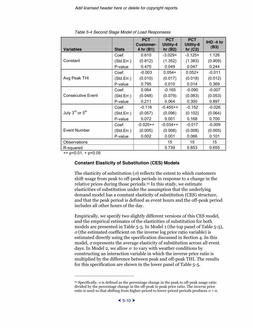
Add licensed header here or delete for copyright reports.
5-10
Table 5-4 Second Stage Model of Load Responsess
Variables Stats
PCT Customer-4 hr (B1)
PCT Utility-4 hr (B2)
PCT Utility-6 hr (C2)
IHD -4 hr (B3)
Constant Coef. 0.610 -3.029+ -3.125+ 1.126 (Std.Err.) (0.812) (1.352) (1.383) (0.909) P-value 0.470 0.049 0.047 0.244
Avg Peak THI Coef. -0.003 0.054+ 0.052+ -0.011 (Std.Err.) (0.010) (0.017) (0.018) (0.012) P-value 0.795 0.010 0.014 0.369
Consecutive Event Coef. 0.064 -0.165 -0.090 -0.007 (Std.Err.) (0.048) (0.079) (0.083) (0.053) P-value 0.211 0.064 0.300 0.897
July 3rd or 5th Coef. -0.116 -0.455++ -0.152 -0.026 (Std.Err.) (0.057) (0.096) (0.102) (0.064) P-value 0.072 0.001 0.168 0.700
Event Number Coef. -0.020++ -0.034++ -0.017 -0.009 (Std.Err.) (0.005) (0.008) (0.008) (0.005) P-value 0.002 0.001 0.066 0.101
Observations 15 15 15 R-squared 0.739 0.853 0.655 ++ p<0.01, + p<0.05
Constant Elasticity of Substitution (CES) Models
The elasticity of substitution ( ) reflects the extent to which customers shift usage from peak to off-peak periods in response to a change in the relative prices during those periods.25 In this study, we estimate elasticities of substitution under the assumption that the underlying demand model has a constant elasticity of substitution (CES) structure, and that the peak period is defined as event hours and the off-peak period includes all other hours of the day.
Empirically, we specify two slightly different versions of this CES model, and the empirical estimates of the elasticities of substitution for both models are presented in Table 5-5. In Model 1 (the top panel of Table 5-5), (the estimated coefficient on the inverse log price ratio variable) is estimated directly using the specification discussed in Section 4. In this model, represents the average elasticity of substitution across all event days. In Model 2, we allow to vary with weather conditions by constructing an interaction variable in which the inverse price ratio is multiplied by the difference between peak and off-peak THI. The results for this specification are shown in the lower panel of Table 5-5.
25 Specifically, is defined as the percentage change in the peak to off-peak usage ratio divided by the percentage change in the off-peak to peak price ratio. The inverse price ratio is used so that shifting from higher-priced to lower-priced periods produces > 0.

5-11
As expected, the results are similar to those for the hourly models, in that the treatment cells fall into two groups. Customers in the utility-controlled PCT treatment group exhibit similar levels of demand response, with an elasticity of substitution of 0.299 for customers with the 4-hour event window and 0.275 for customers with the 6-hour event window (Table 5-5). The elasticities of substitution are smaller for other customer groups, about 0.09 for the customers in both the customer-controlled PCT treatment group and the IHD treatment group. In all cases, the estimated elasticities of substitution are statistically significant.
In the second model, we can test whether the event response varies with weather conditions. The results reported in Table 5-5 indicate that it does for customers in all of the treatment groups, the coefficient on the Log Average Price*Average. This conclusion is based on the statistical significance of the coefficients on the interaction terms between the inverse price ratio and weather variables. Informally speaking, this means that percentage changes in load fall as the weather gets hotter. One explanation is the customers are less willing to shift load from event to non-event hours during periods of extremely hot weather.
To illustrate the magnitudes of the changes in demand responsiveness across weather conditions, we can compare the simulated elasticities of substitution on two event days for customers with a 4-hour event window and with utility controlled PCTs (cell B2). Suppose that the average off-peak THI is 72 on both days, and the cooler event day has a peak THI of 75 while the hotter event day has a peak THI of 80. The simulated elasticity of substitution is approximately 0.34 on the cooler day and 0.22 on the hotter day.26
Daily Elasticity of Demand Model
In addition to the CES models, we formulate daily electricity demand models in order to estimate own-price elasticities of demand (as described in Section 4). These models provide estimates of the extent to which customers change the overall event-day load in response to changes in event day prices, with the response expressed as an own-price elasticity of demand, or daily elasticity of demand ( d).27
26 The elasticity of substitution on a cooler event day is 0.34 = 0.406 + (-0.023* (75 72)). The elasticity of substitution on a hotter event day is 0.22 = 0.406+ (-0.023* (80 72)). 27The daily elasticity is defined as the percentage change in daily usage divided by the percentage change in the daily price.
Add licensed header here or delete for copyright reports.
5-12
Table 5-5 Elasticities of Substitution from CES Models
Control Group versus:
PCT Customer-4
hr (B1)
PCT Utility-4 hr
(B2)
PCT Utility-6 hr
(C2)
IHD -4 hr (B3)
Model 1
Log Inverse Price Ratio
coef. 0.094++ 0.299++ 0.275++ 0.087++ std.err. (0.010) (0.008) (0.008) (0.010) p-value 0.000 0.000 0.000 0.000
Model 2
Log Inverse Price Ratio
coef. 0.174++ 0.406++ 0.416++ 0.138++ std.err. (0.025) (0.018) (0.017) (0.024) p-value 0.000 0.000 0.000 0.000
Log Inverse Price Ratio) *
(Peak THI-Off-peak THI)
coef. -0.017++ -0.023++ -0.029++ -0.011+ std.err. (0.005) (0.004) (0.003) (0.005)
p-value 0.001 0.000 0.000 0.019 Model 2 elasticity at average event-day THI 0.096 0.300 0.275 0.087
++ p<0.01, + p<0.05
The estimated elasticities are shown in Table 5-6. As with the CES models, two versions were estimated. In Model 1 (shown in the top panel of Table 5-6), the daily elasticity is estimated as an average value across all event days. In Model 2 (shown in the bottom panel), the daily demand elasticities are allowed to vary with weather conditions.
The daily demand elasticity estimated in Model 1 is not statistically significant for any treatment group. However, the fact that the point estimates are uniformly negative is consistent with findings from the daily fixed effects models, which found statistically significant event-day conservation for three of the four treatment cells.
The results from Model 2 indicate that the daily elasticity for groups B1 and B3 is sensitive to weather conditions. The positive estimated coefficient on the interaction variable indicates that customers reduce overall usage by a smaller percentage on hotter event days than on milder event days. For example, the daily elasticity for the customer-controlled PCT customers (cell B1) drops from -0.094 to -0.034 as the daily average THI increases from 70 to 75.28 The last row in Tables 5-5 and 5-6 facilitates a comparison of results of the two models by listing the Model 2 elasticity of substitution and demand elasticities, respectively.
28 These value were calculated assuming that the daily elasticity on the cooler event day is -0.094 = -0.934 + (0.012* 70). The daily elasticity on the hotter event day is -0.034 = -0.934 + (0.012 * 75).

5-13
The last row in Tables 5-5 and 5-6 facilitates a comparison of results of the two models by evaluating the Model 2 elasticity of substitution and demand elasticities (respectively) at the mean THI value.
Table 5-6 Daily Demand Elasticities from CES Models
Control Group versus:
PCT Customer-4 hr (B1)
PCT Utility-4 hr (B2)
PCT Utility-6 hr (C2)
IHD -4 hr (B3)
Model 1
Log Average Price
coef. -0.033 -0.018 -0.026 -0.039 std.err. (0.026) (0.020) (0.015) (0.024) p-value 0.194 0.362 0.081 0.111
Model 2
Log Average Price
coef. -0.934+ -0.282 -0.230 -1.021+ std.err. (0.448) (0.317) (0.238) (0.406) p-value 0.037 0.374 0.333 0.012
Log Average Price *
Average THI
coef. 0.012+ 0.004 0.003 0.013+ std.err. (0.006) (0.004) (0.003) (0.005) p-value 0.044 0.405 0.390 0.015
Model 2 elasticity at average event-day THI -0.030 0.019 -0.004 -0.042
++ p<0.01, + p<0.05


6-1
Section 6: Summary and Conclusions Background
FirstEnergy designed its consumer behavior study (CBS) to inform the development of demand response programs that could be deployed to decrease the FirstEnergy Ohio system peak demand and achieve other goals, such as reduced electricity usage at times when supply prices are high or system reliability is in jeopardy. The focal point was to quantify how residential customers respond to an inducement to reduce load during pre-specified hours (ev
The inducement is a payment for reduced usage during events. The payment is an established $/kWh amount applied to the event usage
counterfactual level of usage based on its usage on prior days.
This demand response structure, which is commonly referred to today as a peak-time rebate (PTR), has as antecedents programs implemented by PJM and NYISO beginning in 2000 that involved hundreds of megawatts of load, but primarily from commercial and industrial customers. Earlier versions of this structure, which involve adding a voluntary overlay option to an existing electricity tariff, were implemented through utility pilot programs starting in the early 1990s.
Several pilots implemented in the past few years provided insight into how PTR affects electricity demand, but the results were not conclusive, especially with regard to how the timing and the length of the event influenced event-hour electricity usage adjustments and the extent to which control technologies and feedback augment event response.29
portrayal of how a PTR program would benefit Ohio consumers. The first phase of the CBS was designed to provide a preliminary characterization of how price and technology treatments influenced residential electricity usage. Implementation of the study required the installation of automated metering infrastructure (AMI) to facilitate measuring hourly usage both continuously and during events.
AMI requires adding communication infrastructure characterized by large geographic economies of scale and scope. The study therefore involved homes located in a specific geographic region (outside Cleveland, Ohio). These circuits serve 15,000 customers that comprised the population that was surveyed and produced approximately 5,200 residential premises 29 EPRI 1025856 provides a synthesis of the findings of pilots involving behavioral inducements offered to residential customers to modify their electricity usage.

Add licensed header here or delete for copyright reports.
6-2
where AMI metering was installed and that comprised the customer base for the CBS.
The CBS employed a randomized control trial design to isolate the effects of the PTR price inducements and technology and information, which are the experimental treatments, from other factors that influence residential electricity usage during the course of the year and during periods when PTR events have been declared. The sampling frame from which study participants were drawn was comprised of customers that responded to a survey administered by FirstEnergy at the start of the study.
The customer characteristics survey provided information about the inhabitants that was used to analyze event response and established two foundational subpopulations;; those with central air conditioning and those without. Making this distinction among the sample frame residents was essential because FirstEnergy chose to test (quantify) the effect of a programmable communicating thermostat (PCT) on customer response to PTR inducements. The CBS study therefore involved two separate experiments, one involving a PCT (an enabling control technology) and another involving an in-home display (IHD),(a feedback and information treatment).
The final, two-faceted design involved four treatments;; three combining PCT and PTR and one combining IHD and PTR, and two control groups.
The PTR/PCT experiment also offered treatment options differentiating between four-hour and six-hour events and between customer and FirstEnergy-controlled PCTs. Figure 6-1 illustrates the final design and the number of participants in each treatment and control group.
The treatment cells were populated through recruitment. Offers were extended to eligible customers, separately for the PCT and IHD experiments, until the desired number of subjects was achieved. Control cells were filled by random assignment, removing those customers from the recruitment pool. This was accomplished in the summer and fall of 2011, after which technology was deployed. Fifteen PTR events were called from June 1 to August 31, 2012.
FirstEnergy commissioned EPRI to conduct a preliminary CBS analysis using hourly data for approximately 5,200 customers in the sample frame and data from a second survey administered by FirstEnergy to those customers in the late summer and fall of 2012. EPRI conducted a series of analyses involving graphic depictions of the customer usage by treatment cells, and by applying statistical models to the data to quantify the impacts of the treatments and determine whether they were statistically significant.
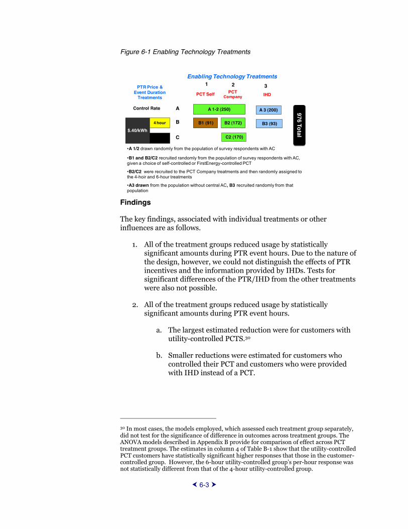
6-3
Figure 6-1 Enabling Technology Treatments
Findings
The key findings, associated with individual treatments or other influences are as follows.
1. All of the treatment groups reduced usage by statistically significant amounts during PTR event hours. Due to the nature of the design, however, we could not distinguish the effects of PTR incentives and the information provided by IHDs. Tests for significant differences of the PTR/IHD from the other treatments were also not possible.
2. All of the treatment groups reduced usage by statistically significant amounts during PTR event hours.
a. The largest estimated reduction were for customers with utility-controlled PCTS.30
b. Smaller reductions were estimated for customers who controlled their PCT and customers who were provided with IHD instead of a PCT.
30 In most cases, the models employed, which assessed each treatment group separately, did not test for the significance of difference in outcomes across treatment groups. The ANOVA models described in Appendix B provide for comparison of effect across PCT treatment groups. The estimates in column 4 of Table B-1 show that the utility-controlled PCT customers have statistically significant higher responses that those in the customer-controlled group. However, the 6-hour utility- -hour response was not statistically different from that of the 4-hour utility-controlled group.
PTR Price & Event Duration
Treatments
Enabling Technology Treatments
$.40/kWh4 hour
6 hour
Control Rate A
B
C
PCT Self PCT Company
A 1-2 (250)
B2 (172)B1 (91)
C2 (170)
1 2
IHD
B3 (93)
A 3 (200)
3
A 1/2 drawn randomly from the population of survey respondents with AC
B1 and B2/C2 recruited randomly from the population of survey respondents with AC, given a choice of self-controlled or FirstEnergy-controlled PCT
B2/C2 were recruited to the PCT Company treatments and then randomly assigned to the 4-hoir and 6-hour treatments
A3 drawn from the population without central AC, B3 recruited randomly from that population
976 Total

Add licensed header here or delete for copyright reports.
6-4
3. The PTR influenced usage in non-event hours on event days.
a. The utility-controlled PCT customers exhibited a substantial rebound effect, an increase in usage (over what would otherwise be expected), during several hours after the event ended.
b. The rebound effect for the 6-hour utility-controlled PCT customers reached a higher single-hour level than it did for the 4-hour utility-controlled PCT customers.
c. However, the total amount of rebound energy for the 6-hour customers was a smaller proportion of the total event-hour usage reductions than it was for the 4-hour customers.
d. Pre-event usage decreased for the PCT self-adjusted group, but not for any other treatment groups.
4. The per-hour usage reductions for the 4-hour and 6-hour utility-controlled PCT customers were very similar, though longer in duration for the customers with 6-hour events.
5. Two of the treatment groups showed evidence of event fatigue, or a reduction in the level of the load impact as the summer progressed, controlling for other factors (e.g., weather conditions).
6. Using a different measure of demand response, the elasticity of substitution (which is a measure of the extent to which customers shift load from peak to off-peak periods), we estimated statistically significant demand response for all four treatment groups and the findings are generally statistically significant.
7. The kWh usage reductions for the utility-controlled PCT customers increased as the weather got hotter. However, the elasticity of substitution declined as the peak-period weather was hotter relative to the off-peak weather.
8. We did not find evidence that usage reductions differed on consecutive event days (i.e., the usage reductions when the event was the second or third in a row did not differ from the usage reductions on initial events).
9. For three of the four treatment groups (i.e., all but the 4-hour utility-controlled PCT customers), we found evidence of a small reduction in total usage on event days.
10. Substitution elasticities, which measure the relative impact of the inducement on event usage ranged in value from 0.09 (customer dispatched PCT) to 0.30 (for FirstEnergy dispatched PCT). The higher values comport with substitution effects reported in the most recently completed DOE-sponsored CBS (EPRI 5856).

6-5
Any interpretation or extension of the study results must account for the structure of the pilot and the analyses that it accommodated.
Specifically, we estimated substitution elasticities to measure the extent to which treatment customers shift usage during PTR events from the event hours to other hours of the day. The purpose was to provide a means of comparing the results to those of other pilots that employed different PTR prices and to be able to forecast customer response at alternative PTR incentive levels. However, one should exercise caution when applying the estimated elasticities to forecast load reductions at PTR incentive levels different from the $0.40 per kWh level used in the CBS.
For the utility-controlled PCT treatment groups, the reduction of AC operation was imposed and few customers overrode that control during events. Therefore, their response (kWh reduction) was largely driven by
characteristics. The same level of response might be realized at lower or higher PTR inducement levels because customers elect to abide by the issued PCT control command that raises the thermostat setting three degrees, regardless of the incentive offered. This autonomous control arrangement may limit the use of the estimated price elasticity to predict how customer would respond to different PCT inducement levels.
In the case of the IHD and customer-controlled PCT treatment groups, it is more appropriate to apply the estimated elasticities of substitution to alternative PTR incentive levels. That is, while the results are still limited by the fact that the CBS contained only one PTR incentive level, the fact that customers in these treatment groups independently determined their response to the PTR incentive makes it more likely that their response would be affected by the magnitude of the PTR incentive.


A-1
Appendix A: Validation of the Data There are generally two types of concerns in the validation of hourly load data such as those used in this CBS. One issue relates to missing values for some customers, while the other relates to identifying extreme values, such as zero, which are likely to be errors in the data.
In the hourly load data made available for this analysis of the load impacts for this CBS, there appeared to be no problems related to missing values.
This was not true, however, in the case of zero and missing values for hourly loads for some customers. This problem was particularly prevalent in some pre-treatment months. For this reason, we concluded that the load data during pre-treatment months could not be used in the analysis. The magnitude of this problem is reflected in Table A-1, which contains summaries of the shares of hourly load observations that are equal to zero during each month for each group of treatment and control customers.

Add licensed header here or delete for copyright reports.
A-2
Table A-1 Share of Zero and Missing Values by Month and Treatment
Month PCT-
Control Group (A1/2)
IHD -Control Group (A3)
PCT Customer-4 hr (B1)
PCT Utility-4 hr (B2)
IHD -4 hr (B3)
PCT Utility-6 hr (C2)
Average
Jun-11 62.2% 80.5% 77.8% 69.6% 88.7% 63.6% 73.7% Jul-11 38.0% 66.2% 53.5% 41.4% 80.2% 40.9% 53.4% Aug-11 16.6% 41.0% 30.6% 17.2% 67.4% 20.0% 32.1% Sep-11 12.5% 27.8% 26.2% 14.4% 63.8% 16.9% 26.9% Oct-11 11.5% 20.7% 19.4% 14.4% 46.2% 16.8% 21.5% Nov-11 2.7% 8.3% 5.5% 4.7% 4.1% 5.1% 5.1% Dec-11 2.8% 11.2% 6.1% 5.2% 7.0% 5.5% 6.3% Jan-12 3.4% 6.3% 6.4% 5.1% 5.3% 6.3% 5.5% Feb-12 4.0% 5.4% 6.3% 6.2% 3.9% 6.8% 5.4% Mar-12 8.9% 10.8% 11.3% 10.5% 9.0% 11.4% 10.3% Apr-12 2.0% 3.3% 2.9% 2.9% 2.1% 4.8% 3.0% May-12 7.2% 10.4% 8.9% 7.9% 7.0% 10.1% 8.6% Jun-12 1.8% 5.5% 0.4% 0.2% 0.4% 0.6% 1.5% Jul-12 1.6% 3.1% 0.0% 0.0% 0.1% 0.0% 0.8% Aug-12 0.8% 3.9% 0.3% 0.0% 0.2% 0.0% 0.9% CBS Period Average
1.4% 4.2% 0.2% 0.1% 0.2% 0.2% 1.1%
Zero values in the data are most prevalent in the earliest months, from June through August 2011, with spikes in the proportions of zero values in later months as well (e.g., March and May 2012). The zero values are often evenly distributed among treatment programs, except for the IHD Control Group (A3), which consistently has higher shares of zeroes.
As also illustrated in Table A-1, load data during the analysis period (summer 2012) contained relatively few zero observations. To ensure that the remaining zeros in the data do not affect the results, however, we excluded from the database any customer if more than two percent of the
non-holiday weekday hourly observations on load between June 1 and August 31, 2012 were zero. Table A-2 contains a list of customers whose electricity usage data are excluded from all models based on this criterion.

A-3
Table A-2 Customers Excluded from the Analysis
CBS Treatment Cell
Customer ID
CBS Treatment Cell
Customer ID
Control- IHD (A3)
1878
Control-PCT (A1/2)
769 1887 1909 2111 2169 2139 3340 2589 3361 2611 4567 3143 4759 3427 4825 3528 5097 3655 PCT Customer-4 hr
(B1)
2134 3969 2832 3991 4426 3996
PCT Utility-4 hr (B2) 574
4195 1687 4264 1903 4506
PCT Utility-6 hr (C2)
2381 4560 2636 4584 4429 4625 4587 4735
IHD -4 hr (B3) 684 2143 4197


B-1
Appendix B: The ANOVA Analyses ANOVA analysis consists of a direct comparison of treatment and control group outcomes to determine whether they are statistically different. For example, we could compare event-hour usage between customer-controlled PCT treatment customers and the PCT control group. If the difference is statistically significant, then we conclude that there is the presence of a treatment effect.
This method, however, only performs well where the control group load serves as a good proxy for the treatment group outcome that would have been observed in the absence of the stimulus. Because we have observed differences in non-event day usage for some treatment and control groups, these conditions may not be fulfilled for many of the comparisons needed for a complete program evaluation. For completeness, however, we have included the ANOVA results below. We present the estimation method below.
The ANOVA analysis was conducted using ordinary least squares (OLS) regressions with indicator variables for each treatment. That is, if a given customer is in a particular treatment group, the indicator variable for that treatment is assigned a value of one for that customer or a value of zero otherwise. This approach facilitates simultaneous comparisons across many treatments. For analytiis measured in three distinct ways:
Average overall usage, a reduction in which serves as a measure of electricity conservation (measured over all non-holiday weekdays, or measured only on event days);;
Average peak-period usage, a reduction in which serves as a measure of demand response (measured over all non-holiday weekdays, or measured only on event days);; and
Peak-to-off-peak usage ratio, a reduction in which serves as a measure of load shifting (measured over all non-holiday weekdays, or measured only on event days).
Each measure is constructed from the hourly kWh usage data, and they are averaged across all customers in each treatment and control group. No weather adjustments are required for ANOVA because all customers experience the same weather conditions and we evaluate all customers using a consistent period of time (e.g., average usage during the summer months).
Because customers in the PCT cells (A1|2, B1, B2, and C2) were sampled differently than customers in IHD treatment cells (A3 and B3), we

Add licensed header here or delete for copyright reports.
B-2
estimate separate models for each group. The effects of IHD technology relative to PCT technology cannot be isolated.
The OLS regression models used in the ANOVA analysis for PCT and IHD customers (respectively) are as follows:31
PCT_Usage i = + PCT_FE x PCT_F Ei + PTR x PTRi + Hr6 x Hr6 + BPTR_Hr6 x PTR_Hr61
+ ec,i
IHD_Usage1 = + PTR x PTR1 + ec,i
where:
i indexes customers;; is the constant term (the usage level for the control group);; The s are estimated parameters (the revealed treatment effects);; PCT_Usagei and IHD_Usagei represent the usage-based value of interest;; PCT_FEi is an indicator variable for FirstEnergy control of the PCT (cells B2 and C2);; PTRi is an indicator variable for being on PTR (all cells except A1|2 and A3);; HR6t is an indicator variable for customers with a 6-hour peak period (C2 customers and A1/2 customers measured across the 6-hour peak);; PTR_HR6t is an indicator variable for customers with a 6-hour peak period who are on PTR (cell C2);; and ei is the error term.
The treatment coefficients may be added to determine cell-level treatment effects as follows:
Customer-controlled PCT (B1) = PTR 4-hour utility-controlled PCT (B2) = PTR + PCT_FE 6-hour utility-controlled PCT (C2) = PTR + PCT_FE + PTR_HR6 IHD customers (B3) = PTR
As described above, ANOVA analyses measure treatment effects using direct comparisons of treatment and control group outcomes. That is, the underlying assumption is that the outcomes for the two groups would be identical but for the stimulus provided to the treatment group. Because treatment customers self-selected into CBS while control-group customers did not, we do not believe that simple treatment versus control group comparisons provide the best estimates of treatment effects. Still, we provide the results of such tests for completeness.
31 Within the PCT model, the control group (A1|2) is duplicated in the sample in order to isolate the effects of a six-hour peak period relative to a four-hour peak period. One set of the duplicated A1|2 customers is treated as having a four-hour peak and the other as having a six-hour peak. Without this construction, it would not be possible to determine whether differences in estimated effects of the six-hour peak period (cell C2) are due to the treatment or the measurement across a different set of hours. Clustered standard errors are used in the PCT ANOVA model to account for the inclusion of duplicated customers.

B-3
A range of outcomes are tested, as follows:
Average usage on all non-holiday weekdays, as a measure of overall conservation;;
Average usage on all event days, as a measure of event-day conservation;;
Average usage during all peak hours, as a measure of overall peak usage changes;;
Average usage during event hours, as a measure of event-period usage changes;;
Peak to off-peak usage ratio on all days, as a measure of load shifting across all days;; and
Peak to off-peak usage on event days, as a measure of load shifting on event days.
Tables B-1 (for PCT customers) and B-2 (for IHD customers) contain the results for each of these measures. The explanatory variables represent the specific stimuli that were given to treatment customers;; the results are summarized as total effects by treatment group in Table B-3.
The results show the following:
No evidence of conservation, either overall or on event days (columns 1 and 2);;
All PCT customers reduced peak usage on PTR event days, and to a lesser extent on all non-holiday weekdays (the PTR coefficient in columns 3 and 4);;
Utility control of the PCT (versus customer control) further decreases peak-period loads (the PCT_FE coefficient in columns 3 and 4);;
Customers with a 6-hour event window and with utility-controlled PCTs do not respond by more than customers with a 4-hour event window and with utility-controlled PCTs (the PTR_Hr6 coefficient in columns 3 and 4);; and
For PCT customers (Table B-1), the results for the event-day peak to off-peak ratio of usage (column 6) follow the same pattern as the event-hour results (column 4);;
IHD customers (Table B-2) do not show any evidence of conservation or peak-period usage differences (columns 1 through 4), but they do show

Add licensed header here or delete for copyright reports.
B-4
differences in the peak to off-peak usage ratio (columns 5 and 6) which indicates the possibility of demand response by these customers.
Table B-1 PCT Results from ANOVA Model
PCT Customer Model where Usage (kWh/hr) is Measured over : (1) (2) (3) (4) (5) (6)
All Non-Holiday
Weekday Hours
All Event Day
Hours All Peak Hours
Event Day Peak
Hours All Days
P/O Ratio Event Day P/O Ratio
Constant Coef. 1.635++ 2.162++ 2.247++ 3.127++ 1.514++ 1.670++
(Std.Err.) (0.068) (0.079) (0.085) (0.102) (0.026) (0.028) P-value 0.000 0.000 0.000 0.000 0.000 0.000
PTR Coef. -0.143 -0.196 -0.280+ -0.515++ -0.092 -0.209++
(Std.Err.) (0.105) (0.125) (0.137) (0.178) (0.052) (0.062) P-value 0.176 0.117 0.041 0.004 0.074 0.001
PCT_FE Coef. 0.063 0.059 -0.039 -0.549++ -0.065 -0.392++
(Std.Err.) (0.096) (0.116) (0.126) (0.166) (0.051) (0.064) P-value 0.511 0.612 0.755 0.001 0.202 0.000
Hr6 Coef. -0.000 -0.000 -0.033++ -0.046++ 0.089++ 0.120++
(Std.Err.) (0.000) (0.000) (0.005) (0.006) (0.006) (0.008) P-value 1.000 1.000 0.000 0.000 0.000 0.000
PTR_Hr6 Coef. 0.027 0.004 0.047 0.126 -0.054 -0.079
(Std.Err.) (0.077) (0.092) (0.098) (0.111) (0.038) (0.042) P-value 0.722 0.970 0.634 0.260 0.157 0.060
Observations 905 905 905 905 905 905 R-squared 0.003 0.005 0.016 0.106 0.053 0.313 Clustered standard errors in parentheses. ++ p<0.01, + p<0.05. There are 241 4-hour and 241 6-hour PCT control group customers (A1/2) included in the model.

B-5
Table B-2 IHD Results from ANOVA Model
IHD Customer Model where Usage (kWh/hr) is Measured over: (1) (2) (3) (4) (5) (6)
All Non-Holiday
Weekday Hours
All Event Day
Hours All Peak Hours
Event Day Peak
Hours All Days
P/O Ratio Event Day P/O Ratio
Constant Coef. 1.207++ 1.391++ 1.415++ 1.668++ 1.239++ 1.271++
(Std.Err.) (0.052) (0.063) (0.068) (0.083) (0.035) (0.037) P-value 0.000 0.000 0.000 0.000 0.000 0.000
PTR Coef. 0.114 0.078 0.053 -0.104 -0.094+ -0.201++
(Std.Err.) (0.098) (0.113) (0.123) (0.146) (0.046) (0.051) P-value 0.246 0.490 0.665 0.477 0.041 0.000
Observations 270 270 270 270 270 270 R-squared 0.005 0.002 0.001 0.002 0.011 0.042 Clustered standard errors in parentheses. ++ p<0.01, + p<0.05. There are 180 IHD control group customers included in the model.
Table B-3 Summary of Cell-Level Treatment Effects from ANOVA Model
Average Hourly Load Changes as Measured by (% in parentheses): (1) (2) (3) (4) (5) (6)
All Non-Holiday
Weekday Hours
All Event Day
Hours
All Peak Hours
Event Day Peak
Hours All Days
P/O Ratio Event
Day P/O Ratio
PCT Customer-4 hr (B1) -0.143 -0.196 -0.280+ -0.515++ -0.092 -0.209++ (-9%) (-9%) (-12%) (-16%) (-6%) (-13%)
PCT Utility-4 hr (B2) -0.080 -0.137 -0.319++ -1.064++ -0.158++ -0.600++ (-5%) (-6%) (-14%) (-34%) (-10%) (-36%)
PCT Utility-6 hr (C2) -0.052 -0.134 -0.273+ -0.938++ -0.211++ -0.679++ (-3%) (-6%) (-12%) (-30%) (-13%) (-38%)
IHD-4 hr (B3) 0.114 0.078 0.053 -0.104 -0.094+ -0.201++ (9%) (6%) (4%) (-6%) (-8%) (-16%)
++ p<0.01, + p<0.05 (based on robust standard errors)

Add licensed header here or delete for copyright reports.
B-6
Because customers self-select into the treatment groups, we believe that the hourly fixed effects models described in Sections 4 and 5 provide more accurate estimates of CBS treatment effects than ANOVA analyses. It may be instructive to summarize the difference between the average event-hour usage changes by treatment group using the two methods.
Table B-4 contains the average estimated event-hour load impacts by method and treatment group.32 The most striking difference is that for three of the four treatment groups, the estimates of the reductions in usage based on the ANOVA model are considerably higher than those estimates based on the hourly fixed effects models for three of the four treatment groups. In contrast to the other three treatments, the estimate of the load reductions for the IHD treatment customers (cell B3) is smaller for the ANOVA model.
This result in some sense validates the observations we made from Figures 4-1 and 4-2. That is, the graphs in Figure 4-1 indicated that usage for customers in the IHD treatment group exceeded usage for the customers in the IHD control group on non-event days. In Figure 4-2, it appeared that the IHD treatment-group customers changed their usage profile on event days, but not to the point that event-hour usage was substantially below that of the IHD control group. Based on these two observations, we would have expected that an ANOVA model would underestimate the reductions in event-hour usage for the IHD treatment group which reflects only differences in event-day usage (shown in Figure 4-2) and does not account for differences in usage on non-event days (shown in Figure 4-1).
Table B-4 Comparison of Estimated Event-Hour Usage Changes, ANOVA and Hourly Fixed Effects Models (kWh per hour)
Treatment Group Hourly Fixed
Effects ANOVA
PCT Customer-4 hr (B1) -0.281 -0.515 PCT Utility-4 hr (B2) -0.814 -1.064 PCT Utility-6 hr (C2) -0.781 -0.938 IHD 4 hr (B3) -0.211 -0.104
32 ANOVA results are from column 4 of Table C-3. Hourly Fixed Effects results are from Table 5-1.

C-1
Appendix C: Detailed Results for all Estimated Fixed Effects Models
Tables C-1 through C-17 contain detailed estimation results for the fixed-effects models that are described in Sections 4 and 5 of the report.

Add licensed header here or delete for copyright reports.
C-2
Table C-1 Fixed-Effects Results for PCT Customers- 4hr (B1) versus PCT Control (Hours 1 through 8)
Variables Stats Hour 1 Hour 2 Hour 3 Hour 4 Hour 5 Hour 6 Hour 7 Hour 8
Constant Coef. -3.420++ -2.664++ -2.009++ -1.542++ -1.307++ -1.044++ -1.072++ -1.179++ (Std.Err.) (0.075) (0.063) (0.055) (0.050) (0.051) (0.052) (0.058) (0.075) P-value 0.000 0.000 0.000 0.000 0.000 0.000 0.000 0.000
Event Coef. 0.026 0.029+ 0.024+ 0.026+ 0.042++ 0.022+ 0.027+ 0.080++ (Std.Err.) (0.016) (0.013) (0.012) (0.010) (0.010) (0.011) (0.013) (0.016) P-value 0.094 0.028 0.035 0.015 0.000 0.046 0.038 0.000
Event*Treat Coef. 0.100++ 0.031 0.021 0.025 0.011 0.028 0.016 -0.053 (Std.Err.) (0.030) (0.025) (0.022) (0.020) (0.020) (0.021) (0.026) (0.031) P-value 0.001 0.217 0.348 0.215 0.571 0.174 0.541 0.087
Tuesday Coef. 0.002 0.012 0.001 0.020 0.044++ 0.042++ 0.033+ 0.066++ (Std.Err.) (0.017) (0.014) (0.013) (0.011) (0.011) (0.011) (0.013) (0.016) P-value 0.905 0.386 0.949 0.075 0.000 0.000 0.015 0.000
Tue*Treat Coef. 0.009 -0.036 -0.015 -0.017 0.005 0.012 0.019 -0.007 (Std.Err.) (0.032) (0.027) (0.024) (0.022) (0.021) (0.022) (0.026) (0.031) P-value 0.775 0.191 0.523 0.426 0.799 0.604 0.453 0.823
Wednesday Coef. 0.113++ 0.091++ 0.083++ 0.096++ 0.093++ 0.071++ 0.067++ 0.067++ (Std.Err.) (0.019) (0.016) (0.014) (0.013) (0.012) (0.013) (0.015) (0.017) P-value 0.000 0.000 0.000 0.000 0.000 0.000 0.000 0.000
Wed*Treat Coef. 0.019 0.016 0.004 0.016 0.037 0.028 0.019 0.016 (Std.Err.) (0.036) (0.030) (0.026) (0.024) (0.023) (0.025) (0.029) (0.034) P-value 0.594 0.604 0.891 0.509 0.116 0.253 0.509 0.628
Thursday Coef. 0.051++ 0.066++ 0.052++ 0.057++ 0.066++ 0.061++ 0.065++ 0.053++ (Std.Err.) (0.018) (0.015) (0.013) (0.012) (0.012) (0.012) (0.015) (0.017) P-value 0.005 0.000 0.000 0.000 0.000 0.000 0.000 0.002
Thu*Treat Coef. 0.024 -0.005 0.006 -0.001 0.003 0.009 0.013 -0.019 (Std.Err.) (0.035) (0.030) (0.026) (0.024) (0.023) (0.024) (0.028) (0.033) P-value 0.502 0.860 0.804 0.970 0.892 0.706 0.649 0.569
Friday Coef. 0.006 0.016 0.023 0.038++ 0.047++ 0.034++ 0.025 0.033+ (Std.Err.) (0.017) (0.014) (0.012) (0.011) (0.011) (0.011) (0.013) (0.016) P-value 0.720 0.264 0.066 0.001 0.000 0.003 0.063 0.039
Fri*Treat Coef. 0.016 -0.004 -0.009 0.018 0.005 -0.020 0.004 -0.055 (Std.Err.) (0.033) (0.027) (0.024) (0.021) (0.021) (0.022) (0.026) (0.031) P-value 0.627 0.880 0.705 0.401 0.803 0.373 0.876 0.072
THI Coef. 0.048++ 0.034++ 0.028++ 0.022++ 0.014++ 0.014++ 0.012++ 0.005++ (Std.Err.) (0.002) (0.002) (0.002) (0.001) (0.001) (0.002) (0.002) (0.002) P-value 0.000 0.000 0.000 0.000 0.000 0.000 0.000 0.010
THI*Treat Coef. -0.007 -0.004 -0.003 -0.004 -0.004 -0.003 0.000 0.006 (Std.Err.) (0.004) (0.003) (0.003) (0.003) (0.003) (0.003) (0.004) (0.004) P-value 0.075 0.265 0.399 0.140 0.094 0.293 0.930 0.130
THI MA(24) Coef. 0.018++ 0.021++ 0.017++ 0.015++ 0.018++ 0.014++ 0.017++ 0.028++ (Std.Err.) (0.003) (0.002) (0.002) (0.002) (0.002) (0.002) (0.002) (0.002)

C-3
P-value 0.000 0.000 0.000 0.000 0.000 0.000 0.000 0.000
THI MA(24)*Treat Coef. 0.016++ 0.004 -0.000 -0.001 0.004 0.005 0.005 -0.005 (Std.Err.) (0.005) (0.004) (0.004) (0.003) (0.004) (0.004) (0.004) (0.004) P-value 0.001 0.364 0.926 0.830 0.325 0.241 0.208 0.157
Observations 21,056 21,056 21,056 21,056 21,056 21,056 21,056 21,056 Number of Customers 329 329 329 329 329 329 329 329 R-squared (overall) 0.0372 0.0594 0.0495 0.0366 0.0322 0.0188 0.00800 0.0212 ++ p<0.01, + p<0.05. There are 241 PCT control group customers (A1/2) included in the models.
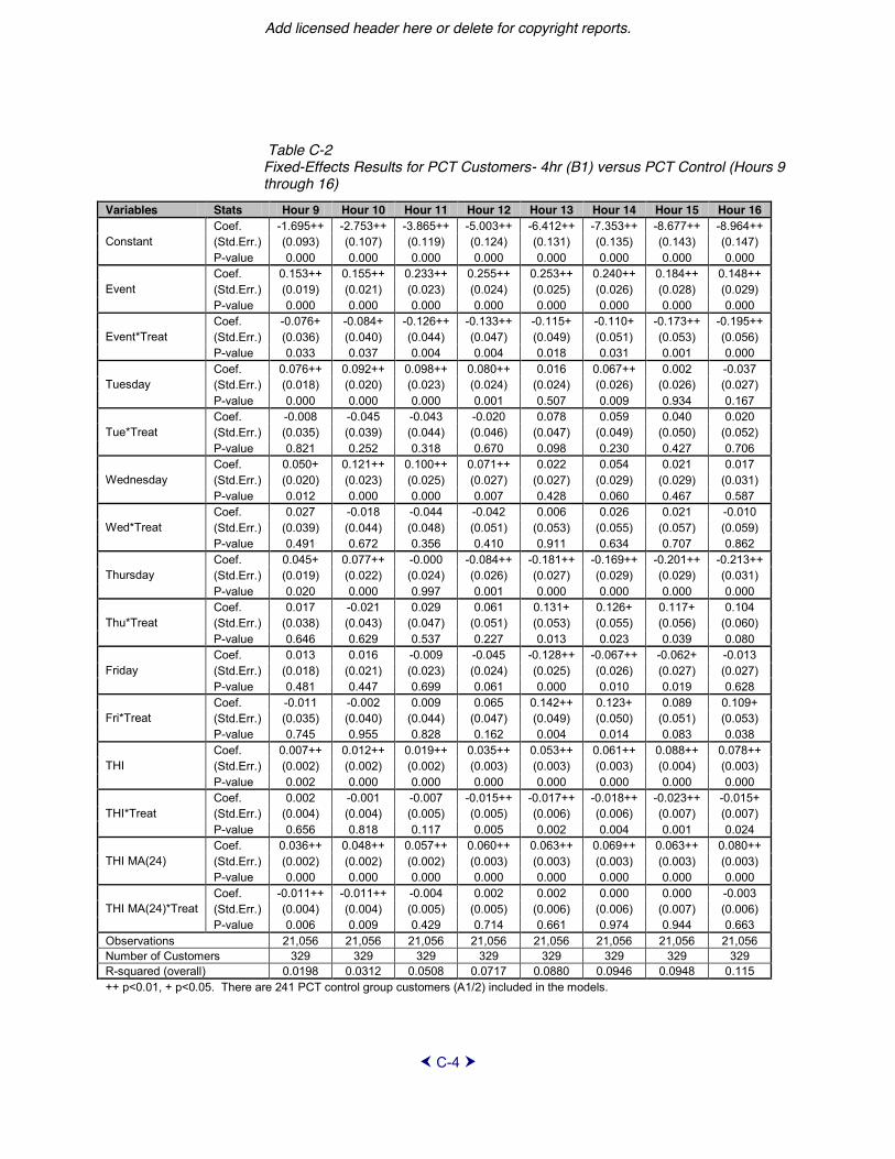
Add licensed header here or delete for copyright reports.
C-4
Table C-2 Fixed-Effects Results for PCT Customers- 4hr (B1) versus PCT Control (Hours 9 through 16)
Variables Stats Hour 9 Hour 10 Hour 11 Hour 12 Hour 13 Hour 14 Hour 15 Hour 16
Constant Coef. -1.695++ -2.753++ -3.865++ -5.003++ -6.412++ -7.353++ -8.677++ -8.964++ (Std.Err.) (0.093) (0.107) (0.119) (0.124) (0.131) (0.135) (0.143) (0.147) P-value 0.000 0.000 0.000 0.000 0.000 0.000 0.000 0.000
Event Coef. 0.153++ 0.155++ 0.233++ 0.255++ 0.253++ 0.240++ 0.184++ 0.148++ (Std.Err.) (0.019) (0.021) (0.023) (0.024) (0.025) (0.026) (0.028) (0.029) P-value 0.000 0.000 0.000 0.000 0.000 0.000 0.000 0.000
Event*Treat Coef. -0.076+ -0.084+ -0.126++ -0.133++ -0.115+ -0.110+ -0.173++ -0.195++ (Std.Err.) (0.036) (0.040) (0.044) (0.047) (0.049) (0.051) (0.053) (0.056) P-value 0.033 0.037 0.004 0.004 0.018 0.031 0.001 0.000
Tuesday Coef. 0.076++ 0.092++ 0.098++ 0.080++ 0.016 0.067++ 0.002 -0.037 (Std.Err.) (0.018) (0.020) (0.023) (0.024) (0.024) (0.026) (0.026) (0.027) P-value 0.000 0.000 0.000 0.001 0.507 0.009 0.934 0.167
Tue*Treat Coef. -0.008 -0.045 -0.043 -0.020 0.078 0.059 0.040 0.020 (Std.Err.) (0.035) (0.039) (0.044) (0.046) (0.047) (0.049) (0.050) (0.052) P-value 0.821 0.252 0.318 0.670 0.098 0.230 0.427 0.706
Wednesday Coef. 0.050+ 0.121++ 0.100++ 0.071++ 0.022 0.054 0.021 0.017 (Std.Err.) (0.020) (0.023) (0.025) (0.027) (0.027) (0.029) (0.029) (0.031) P-value 0.012 0.000 0.000 0.007 0.428 0.060 0.467 0.587
Wed*Treat Coef. 0.027 -0.018 -0.044 -0.042 0.006 0.026 0.021 -0.010 (Std.Err.) (0.039) (0.044) (0.048) (0.051) (0.053) (0.055) (0.057) (0.059) P-value 0.491 0.672 0.356 0.410 0.911 0.634 0.707 0.862
Thursday Coef. 0.045+ 0.077++ -0.000 -0.084++ -0.181++ -0.169++ -0.201++ -0.213++ (Std.Err.) (0.019) (0.022) (0.024) (0.026) (0.027) (0.029) (0.029) (0.031) P-value 0.020 0.000 0.997 0.001 0.000 0.000 0.000 0.000
Thu*Treat Coef. 0.017 -0.021 0.029 0.061 0.131+ 0.126+ 0.117+ 0.104 (Std.Err.) (0.038) (0.043) (0.047) (0.051) (0.053) (0.055) (0.056) (0.060) P-value 0.646 0.629 0.537 0.227 0.013 0.023 0.039 0.080
Friday Coef. 0.013 0.016 -0.009 -0.045 -0.128++ -0.067++ -0.062+ -0.013 (Std.Err.) (0.018) (0.021) (0.023) (0.024) (0.025) (0.026) (0.027) (0.027) P-value 0.481 0.447 0.699 0.061 0.000 0.010 0.019 0.628
Fri*Treat Coef. -0.011 -0.002 0.009 0.065 0.142++ 0.123+ 0.089 0.109+ (Std.Err.) (0.035) (0.040) (0.044) (0.047) (0.049) (0.050) (0.051) (0.053) P-value 0.745 0.955 0.828 0.162 0.004 0.014 0.083 0.038
THI Coef. 0.007++ 0.012++ 0.019++ 0.035++ 0.053++ 0.061++ 0.088++ 0.078++ (Std.Err.) (0.002) (0.002) (0.002) (0.003) (0.003) (0.003) (0.004) (0.003) P-value 0.002 0.000 0.000 0.000 0.000 0.000 0.000 0.000
THI*Treat Coef. 0.002 -0.001 -0.007 -0.015++ -0.017++ -0.018++ -0.023++ -0.015+ (Std.Err.) (0.004) (0.004) (0.005) (0.005) (0.006) (0.006) (0.007) (0.007) P-value 0.656 0.818 0.117 0.005 0.002 0.004 0.001 0.024
THI MA(24) Coef. 0.036++ 0.048++ 0.057++ 0.060++ 0.063++ 0.069++ 0.063++ 0.080++ (Std.Err.) (0.002) (0.002) (0.002) (0.003) (0.003) (0.003) (0.003) (0.003) P-value 0.000 0.000 0.000 0.000 0.000 0.000 0.000 0.000
THI MA(24)*Treat Coef. -0.011++ -0.011++ -0.004 0.002 0.002 0.000 0.000 -0.003 (Std.Err.) (0.004) (0.004) (0.005) (0.005) (0.006) (0.006) (0.007) (0.006) P-value 0.006 0.009 0.429 0.714 0.661 0.974 0.944 0.663
Observations 21,056 21,056 21,056 21,056 21,056 21,056 21,056 21,056 Number of Customers 329 329 329 329 329 329 329 329 R-squared (overall) 0.0198 0.0312 0.0508 0.0717 0.0880 0.0946 0.0948 0.115 ++ p<0.01, + p<0.05. There are 241 PCT control group customers (A1/2) included in the models.

C-5
Table C-3 Fixed-Effects Results for PCT Customers- 4hr (B1) versus PCT Control (Hours 17 through 24)
Variables Stats Hour 17 Hour 18 Hour 19 Hour 20 Hour 21 Hour 22 Hour 23 Hour 24
Constant Coef. -9.903++ -10.581++ -9.878++ -8.288++ -6.571++ -5.012++ -4.545++ -3.981++ (Std.Err.) (0.160) (0.164) (0.161) (0.152) (0.142) (0.133) (0.120) (0.106) P-value 0.000 0.000 0.000 0.000 0.000 0.000 0.000 0.000
Event Coef. 0.110++ 0.070+ 0.093++ 0.177++ 0.215++ 0.235++ 0.200++ 0.131++ (Std.Err.) (0.030) (0.031) (0.030) (0.029) (0.028) (0.026) (0.024) (0.021) P-value 0.000 0.023 0.002 0.000 0.000 0.000 0.000 0.000
Event*Treat Coef. -0.263++ -0.261++ -0.043 0.046 0.104 0.072 0.023 0.068 (Std.Err.) (0.058) (0.060) (0.059) (0.057) (0.054) (0.051) (0.047) (0.041) P-value 0.000 0.000 0.467 0.416 0.053 0.159 0.629 0.101
Tuesday Coef. -0.030 -0.046 -0.025 -0.032 0.046 0.057+ 0.040 0.060++ (Std.Err.) (0.028) (0.029) (0.028) (0.028) (0.027) (0.026) (0.023) (0.020) P-value 0.280 0.109 0.368 0.243 0.086 0.027 0.089 0.003
Tue*Treat Coef. -0.098 -0.095 -0.014 0.018 -0.022 -0.053 -0.009 -0.022 (Std.Err.) (0.054) (0.056) (0.055) (0.054) (0.052) (0.050) (0.045) (0.040) P-value 0.070 0.088 0.794 0.733 0.679 0.282 0.838 0.583
Wednesday Coef. 0.057 0.047 0.035 -0.024 0.063+ 0.075++ 0.036 0.043 (Std.Err.) (0.032) (0.032) (0.032) (0.031) (0.030) (0.028) (0.026) (0.023) P-value 0.072 0.146 0.274 0.447 0.032 0.008 0.165 0.057
Wed*Treat Coef. -0.059 -0.027 0.015 -0.005 -0.024 -0.014 0.041 0.017 (Std.Err.) (0.061) (0.063) (0.061) (0.060) (0.057) (0.054) (0.050) (0.044) P-value 0.331 0.663 0.810 0.935 0.671 0.794 0.406 0.702
Thursday Coef. -0.173++ -0.151++ -0.135++ -0.162++ -0.124++ -0.075++ -0.086++ -0.018 (Std.Err.) (0.032) (0.032) (0.031) (0.030) (0.029) (0.027) (0.026) (0.022) P-value 0.000 0.000 0.000 0.000 0.000 0.007 0.001 0.408
Thu*Treat Coef. -0.020 -0.046 0.009 0.000 -0.017 -0.027 0.018 -0.019 (Std.Err.) (0.061) (0.062) (0.060) (0.059) (0.056) (0.053) (0.049) (0.043) P-value 0.747 0.461 0.878 0.998 0.768 0.614 0.723 0.663
Friday Coef. -0.047 -0.069+ -0.133++ -0.168++ -0.100++ -0.060+ 0.003 0.110++ (Std.Err.) (0.028) (0.029) (0.029) (0.028) (0.027) (0.026) (0.024) (0.021) P-value 0.099 0.017 0.000 0.000 0.000 0.023 0.899 0.000
Fri*Treat Coef. 0.075 0.086 0.081 0.007 -0.060 -0.068 -0.103+ -0.099+ (Std.Err.) (0.055) (0.056) (0.055) (0.054) (0.053) (0.051) (0.046) (0.041) P-value 0.171 0.126 0.144 0.895 0.255 0.186 0.025 0.015
THI Coef. 0.086++ 0.098++ 0.099++ 0.097++ 0.088++ 0.081++ 0.073++ 0.062++ (Std.Err.) (0.003) (0.003) (0.003) (0.003) (0.003) (0.003) (0.003) (0.002) P-value 0.000 0.000 0.000 0.000 0.000 0.000 0.000 0.000
THI*Treat Coef. -0.007 -0.004 -0.000 -0.001 -0.002 -0.003 -0.010 -0.010+ (Std.Err.) (0.007) (0.006) (0.007) (0.007) (0.006) (0.006) (0.006) (0.005) P-value 0.309 0.550 0.968 0.846 0.727 0.672 0.074 0.034
THI MA(24) Coef. 0.085++ 0.084++ 0.073++ 0.052++ 0.035++ 0.018++ 0.015++ 0.015++ (Std.Err.) (0.003) (0.003) (0.003) (0.004) (0.004) (0.004) (0.004) (0.003) P-value 0.000 0.000 0.000 0.000 0.000 0.000 0.000 0.000
THI MA(24)*Treat Coef. -0.003 0.003 -0.001 0.001 0.005 0.011 0.025++ 0.019++ (Std.Err.) (0.006) (0.006) (0.007) (0.007) (0.007) (0.007) (0.007) (0.006) P-value 0.695 0.612 0.906 0.831 0.442 0.133 0.000 0.002
Observations 21,056 21,056 21,056 21,056 21,056 21,056 21,056 21,056 Number of Customers 329 329 329 329 329 329 329 329 R-squared (overall) 0.138 0.149 0.148 0.138 0.112 0.0781 0.0472 0.0507 ++ p<0.01, + p<0.05. There are 241 PCT control group customers (A1/2) included in the models.
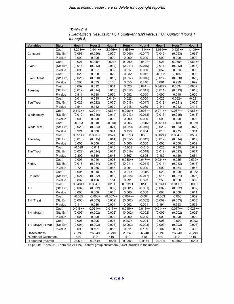
Add licensed header here or delete for copyright reports.
C-6
Table C-4 Fixed-Effects Results for PCT Utility-4hr (B2) versus PCT Control (Hours 1 through 8)
Variables Stats Hour 1 Hour 2 Hour 3 Hour 4 Hour 5 Hour 6 Hour 7 Hour 8
Constant Coef. -3.291++ -2.644++ -2.056++ -1.653++ -1.314++ -1.085++ -0.933++ -1.109++ (Std.Err.) (0.068) (0.056) (0.050) (0.046) (0.047) (0.046) (0.053) (0.069) P-value 0.000 0.000 0.000 0.000 0.000 0.000 0.000 0.000
Event Coef. 0.027 0.029+ 0.024+ 0.026+ 0.042++ 0.021 0.030+ 0.081++ (Std.Err.) (0.016) (0.013) (0.012) (0.011) (0.010) (0.011) (0.013) (0.016) P-value 0.090 0.027 0.039 0.017 0.000 0.052 0.023 0.000
Event*Treat Coef. 0.026 0.020 0.029 0.032 0.012 -0.002 -0.002 0.003 (Std.Err.) (0.025) (0.020) (0.018) (0.017) (0.016) (0.017) (0.020) (0.025) P-value 0.288 0.333 0.106 0.055 0.446 0.891 0.929 0.892
Tuesday Coef. 0.002 0.012 0.001 0.020 0.044++ 0.042++ 0.033+ 0.066++ (Std.Err.) (0.017) (0.014) (0.013) (0.012) (0.011) (0.011) (0.013) (0.016) P-value 0.911 0.388 0.950 0.082 0.000 0.000 0.015 0.000
Tue*Treat Coef. 0.016 0.035 0.043+ 0.022 0.000 0.026 0.052+ -0.021 (Std.Err.) (0.026) (0.022) (0.020) (0.018) (0.017) (0.018) (0.021) (0.025) P-value 0.544 0.112 0.030 0.218 0.979 0.141 0.013 0.413
Wednesday Coef. 0.113++ 0.091++ 0.083++ 0.096++ 0.093++ 0.071++ 0.067++ 0.066++ (Std.Err.) (0.019) (0.016) (0.014) (0.013) (0.013) (0.013) (0.015) (0.018) P-value 0.000 0.000 0.000 0.000 0.000 0.000 0.000 0.000
Wed*Treat Coef. -0.003 0.010 -0.000 0.006 -0.002 0.051++ -0.001 -0.029 (Std.Err.) (0.029) (0.024) (0.021) (0.020) (0.019) (0.020) (0.023) (0.028) P-value 0.921 0.688 0.991 0.750 0.904 0.010 0.975 0.301
Thursday Coef. 0.051++ 0.066++ 0.052++ 0.057++ 0.066++ 0.062++ 0.064++ 0.053++ (Std.Err.) (0.018) (0.015) (0.014) (0.012) (0.012) (0.012) (0.014) (0.017) P-value 0.006 0.000 0.000 0.000 0.000 0.000 0.000 0.002
Thu*Treat Coef. -0.029 -0.011 0.010 -0.008 -0.010 0.026 0.035 0.012 (Std.Err.) (0.029) (0.024) (0.021) (0.019) (0.019) (0.019) (0.023) (0.027) P-value 0.309 0.640 0.648 0.667 0.605 0.182 0.120 0.654
Friday Coef. 0.006 0.016 0.023 0.038++ 0.047++ 0.034++ 0.025 0.032+ (Std.Err.) (0.017) (0.014) (0.012) (0.011) (0.011) (0.011) (0.013) (0.016) P-value 0.729 0.265 0.067 0.001 0.000 0.002 0.064 0.043
Fri*Treat Coef. 0.005 0.018 0.028 0.019 -0.008 0.020 0.009 -0.022 (Std.Err.) (0.027) (0.022) (0.019) (0.018) (0.017) (0.018) (0.021) (0.025) P-value 0.862 0.426 0.154 0.291 0.623 0.250 0.650 0.382
THI Coef. 0.048++ 0.034++ 0.028++ 0.022++ 0.014++ 0.014++ 0.011++ 0.005+ (Std.Err.) (0.002) (0.002) (0.002) (0.001) (0.001) (0.002) (0.002) (0.002) P-value 0.000 0.000 0.000 0.000 0.000 0.000 0.000 0.011
THI*Treat Coef. -0.005 -0.006+ -0.007++ -0.007++ -0.004 -0.003 -0.000 0.002 (Std.Err.) (0.003) (0.003) (0.002) (0.002) (0.002) (0.002) (0.003) (0.003) P-value 0.114 0.036 0.004 0.002 0.051 0.194 0.993 0.572
THI MA(24) Coef. 0.018++ 0.021++ 0.017++ 0.015++ 0.018++ 0.014++ 0.017++ 0.028++ (Std.Err.) (0.003) (0.002) (0.002) (0.002) (0.002) (0.002) (0.002) (0.002) P-value 0.000 0.000 0.000 0.000 0.000 0.000 0.000 0.000
THI MA(24)*Treat Coef. 0.007 0.005 0.006 0.007+ 0.004 0.005 -0.000 -0.003 (Std.Err.) (0.004) (0.003) (0.003) (0.003) (0.003) (0.003) (0.003) (0.003) P-value 0.096 0.191 0.058 0.011 0.159 0.107 0.955 0.300
Observations 26,240 26,240 26,240 26,240 26,240 26,240 26,240 26,240 Number of Customers 410 410 410 410 410 410 410 410 R-squared (overall) 0.0692 0.0640 0.0535 0.0383 0.0334 0.0194 0.0192 0.0208 ++ p<0.01, + p<0.05. There are 241 PCT control group customers (A1/2) included in the models.

C-7
Table C-5 Fixed-Effects Results for PCT Utility-4hr (B2) versus PCT Control (Hours 9 through 16)
Variables Stats Hour 9 Hour 10 Hour 11 Hour 12 Hour 13 Hour 14 Hour 15 Hour 16
Constant Coef. -1.791++ -2.830++ -3.910++ -5.050++ -6.437++ -7.309++ -8.062++ -8.407++ (Std.Err.) (0.086) (0.099) (0.110) (0.115) (0.119) (0.123) (0.129) (0.134) P-value 0.000 0.000 0.000 0.000 0.000 0.000 0.000 0.000
Event Coef. 0.154++ 0.155++ 0.234++ 0.257++ 0.254++ 0.241++ 0.187++ 0.148++ (Std.Err.) (0.019) (0.021) (0.023) (0.025) (0.025) (0.027) (0.027) (0.029) P-value 0.000 0.000 0.000 0.000 0.000 0.000 0.000 0.000
Event*Treat Coef. -0.004 0.031 -0.018 -0.011 0.025 0.099+ -1.034++ -0.995++ (Std.Err.) (0.030) (0.033) (0.036) (0.039) (0.040) (0.041) (0.042) (0.045) P-value 0.885 0.353 0.613 0.777 0.532 0.016 0.000 0.000
Tuesday Coef. 0.076++ 0.092++ 0.098++ 0.079++ 0.016 0.067++ 0.001 -0.038 (Std.Err.) (0.019) (0.021) (0.023) (0.025) (0.025) (0.026) (0.026) (0.027) P-value 0.000 0.000 0.000 0.001 0.528 0.010 0.982 0.158
Tue*Treat Coef. -0.002 -0.027 -0.017 -0.024 0.021 -0.054 -0.005 -0.043 (Std.Err.) (0.029) (0.033) (0.036) (0.038) (0.039) (0.040) (0.041) (0.042) P-value 0.946 0.405 0.638 0.531 0.581 0.180 0.901 0.316
Wednesday Coef. 0.050+ 0.121++ 0.100++ 0.071++ 0.022 0.054 0.023 0.019 (Std.Err.) (0.021) (0.023) (0.025) (0.027) (0.028) (0.029) (0.029) (0.030) P-value 0.015 0.000 0.000 0.009 0.435 0.061 0.435 0.531
Wed*Treat Coef. 0.015 -0.062 -0.067 -0.065 -0.057 -0.031 0.004 -0.051 (Std.Err.) (0.032) (0.036) (0.040) (0.042) (0.043) (0.045) (0.045) (0.047) P-value 0.629 0.084 0.093 0.127 0.190 0.497 0.933 0.278
Thursday Coef. 0.045+ 0.077++ -0.001 -0.084++ -0.182++ -0.170++ -0.204++ -0.215++ (Std.Err.) (0.020) (0.023) (0.025) (0.027) (0.027) (0.029) (0.029) (0.031) P-value 0.025 0.001 0.981 0.002 0.000 0.000 0.000 0.000
Thu*Treat Coef. -0.019 -0.057 -0.002 0.016 0.041 -0.051 0.081 0.089 (Std.Err.) (0.031) (0.035) (0.039) (0.042) (0.043) (0.045) (0.045) (0.048) P-value 0.547 0.106 0.951 0.707 0.342 0.253 0.073 0.063
Friday Coef. 0.013 0.015 -0.009 -0.046 -0.129++ -0.067+ -0.064+ -0.016 (Std.Err.) (0.019) (0.021) (0.023) (0.025) (0.026) (0.026) (0.027) (0.028) P-value 0.501 0.466 0.695 0.064 0.000 0.010 0.015 0.571
Fri*Treat Coef. 0.003 0.020 0.042 0.006 0.022 0.027 0.042 0.049 (Std.Err.) (0.029) (0.033) (0.036) (0.039) (0.040) (0.041) (0.041) (0.043) P-value 0.920 0.540 0.246 0.871 0.584 0.502 0.308 0.253
THI Coef. 0.007++ 0.012++ 0.019++ 0.034++ 0.053++ 0.061++ 0.088++ 0.077++ (Std.Err.) (0.002) (0.002) (0.003) (0.003) (0.003) (0.003) (0.003) (0.003) P-value 0.003 0.000 0.000 0.000 0.000 0.000 0.000 0.000
THI*Treat Coef. 0.002 0.001 0.008+ 0.000 -0.005 -0.002 -0.013+ -0.011+ (Std.Err.) (0.004) (0.004) (0.004) (0.004) (0.004) (0.005) (0.005) (0.005) P-value 0.648 0.824 0.041 0.910 0.261 0.755 0.017 0.038
THI MA(24) Coef. 0.036++ 0.048++ 0.057++ 0.060++ 0.063++ 0.069++ 0.064++ 0.080++ (Std.Err.) (0.002) (0.002) (0.003) (0.003) (0.003) (0.003) (0.003) (0.003) P-value 0.000 0.000 0.000 0.000 0.000 0.000 0.000 0.000
THI MA(24)*Treat Coef. -0.003 -0.005 -0.013++ -0.005 -0.002 -0.010+ -0.021++ -0.019++ (Std.Err.) (0.003) (0.003) (0.004) (0.004) (0.005) (0.005) (0.005) (0.005) P-value 0.301 0.142 0.001 0.225 0.698 0.048 0.000 0.000
Observations 26,240 26,240 26,240 26,240 26,240 26,240 26,240 26,240 Number of Customers 410 410 410 410 410 410 410 410 R-squared (overall) 0.0350 0.0454 0.0630 0.0859 0.106 0.107 0.0652 0.0700 ++ p<0.01, + p<0.05. There are 241 PCT control group customers (A1/2) included in the models.

Add licensed header here or delete for copyright reports.
C-8
Table C-6 Fixed-Effects Results for PCT Utility-4hr (B2) versus PCT Control (Hours 17 through 24)
Variables Stats Hour 17 Hour 18 Hour 19 Hour 20 Hour 21 Hour 22 Hour 23 Hour 24
Constant Coef. -9.583++ -10.215++ -9.464++ -7.823++ -6.078++ -4.885++ -4.185++ -3.730++ (Std.Err.) (0.146) (0.147) (0.143) (0.136) (0.127) (0.121) (0.109) (0.095) P-value 0.000 0.000 0.000 0.000 0.000 0.000 0.000 0.000
Event Coef. 0.111++ 0.070+ 0.093++ 0.177++ 0.215++ 0.235++ 0.200++ 0.131++ (Std.Err.) (0.030) (0.031) (0.030) (0.029) (0.028) (0.027) (0.024) (0.021) P-value 0.000 0.021 0.002 0.000 0.000 0.000 0.000 0.000
Event*Treat Coef. -0.793++ -0.556++ 0.687++ 0.636++ 0.481++ 0.283++ 0.157++ 0.145++ (Std.Err.) (0.047) (0.048) (0.047) (0.046) (0.044) (0.042) (0.038) (0.033) P-value 0.000 0.000 0.000 0.000 0.000 0.000 0.000 0.000
Tuesday Coef. -0.032 -0.047 -0.025 -0.032 0.047 0.057+ 0.040 0.060++ (Std.Err.) (0.028) (0.029) (0.028) (0.028) (0.027) (0.026) (0.024) (0.021) P-value 0.262 0.100 0.369 0.245 0.083 0.029 0.092 0.004
Tue*Treat Coef. -0.032 -0.019 0.016 0.021 -0.009 0.025 -0.015 0.013 (Std.Err.) (0.044) (0.045) (0.044) (0.043) (0.042) (0.041) (0.037) (0.032) P-value 0.475 0.669 0.709 0.634 0.839 0.534 0.678 0.675
Wednesday Coef. 0.058 0.047 0.035 -0.024 0.064+ 0.075++ 0.036 0.043 (Std.Err.) (0.032) (0.032) (0.032) (0.031) (0.030) (0.028) (0.026) (0.023) P-value 0.066 0.141 0.272 0.444 0.032 0.009 0.168 0.058
Wed*Treat Coef. -0.043 -0.039 -0.006 -0.008 -0.025 -0.000 -0.013 -0.014 (Std.Err.) (0.049) (0.050) (0.049) (0.048) (0.046) (0.044) (0.041) (0.035) P-value 0.383 0.431 0.910 0.866 0.589 0.994 0.753 0.684
Thursday Coef. -0.175++ -0.152++ -0.134++ -0.161++ -0.124++ -0.074++ -0.086++ -0.018 (Std.Err.) (0.032) (0.032) (0.031) (0.030) (0.029) (0.028) (0.026) (0.022) P-value 0.000 0.000 0.000 0.000 0.000 0.008 0.001 0.411
Thu*Treat Coef. 0.043 -0.021 0.052 0.015 -0.014 0.012 0.030 0.021 (Std.Err.) (0.049) (0.049) (0.048) (0.047) (0.046) (0.044) (0.040) (0.035) P-value 0.388 0.671 0.283 0.745 0.759 0.778 0.454 0.557
Friday Coef. -0.049 -0.071+ -0.132++ -0.168++ -0.100++ -0.059+ 0.003 0.110++ (Std.Err.) (0.029) (0.029) (0.028) (0.028) (0.027) (0.027) (0.024) (0.021) P-value 0.087 0.013 0.000 0.000 0.000 0.026 0.903 0.000
Fri*Treat Coef. 0.102+ 0.092+ 0.052 0.015 -0.019 -0.008 -0.015 0.010 (Std.Err.) (0.045) (0.045) (0.044) (0.044) (0.043) (0.042) (0.037) (0.033) P-value 0.022 0.041 0.238 0.735 0.658 0.840 0.697 0.754
THI Coef. 0.086++ 0.097++ 0.099++ 0.097++ 0.088++ 0.081++ 0.073++ 0.062++ (Std.Err.) (0.003) (0.003) (0.003) (0.003) (0.003) (0.003) (0.003) (0.002) P-value 0.000 0.000 0.000 0.000 0.000 0.000 0.000 0.000
THI*Treat Coef. -0.009 -0.013++ -0.028++ -0.024++ -0.017++ -0.016++ -0.014++ -0.009+ (Std.Err.) (0.005) (0.005) (0.005) (0.005) (0.005) (0.005) (0.005) (0.004) P-value 0.082 0.007 0.000 0.000 0.000 0.001 0.002 0.023
THI MA(24) Coef. 0.085++ 0.084++ 0.073++ 0.052++ 0.035++ 0.018++ 0.015++ 0.015++ (Std.Err.) (0.003) (0.003) (0.003) (0.004) (0.004) (0.004) (0.004) (0.003) P-value 0.000 0.000 0.000 0.000 0.000 0.000 0.000 0.000
THI MA(24)*Treat Coef. -0.007 0.001 0.014+ 0.008 0.002 0.017++ 0.010 0.005 (Std.Err.) (0.005) (0.005) (0.005) (0.006) (0.006) (0.006) (0.006) (0.005) P-value 0.185 0.808 0.011 0.180 0.723 0.006 0.066 0.302
Observations 26,240 26,240 26,240 26,240 26,240 26,240 26,240 26,240 Number of Customers 410 410 410 410 410 410 410 410 R-squared (overall) 0.0979 0.115 0.133 0.111 0.0825 0.110 0.0897 0.0797 ++ p<0.01, + p<0.05. There are 241 PCT control group customers (A1/2) included in the models.

C-9
Table C-7 Fixed-Effects Results for PCT Utility-6hr (C2) versus PCT Control (Hours 1 through 8)
Variables Stats Hour 1 Hour 2 Hour 3 Hour 4 Hour 5 Hour 6 Hour 7 Hour 8
Constant Coef. -3.243++ -2.516++ -1.960++ -1.563++ -1.198++ -0.940++ -0.889++ -0.943++ (Std.Err.) (0.070) (0.060) (0.050) (0.045) (0.051) (0.059) (0.069) (0.095) P-value 0.000 0.000 0.000 0.000 0.000 0.000 0.000 0.000
Event Coef. 0.027 0.030+ 0.023 0.024+ 0.043++ 0.023 0.033+ 0.086++ (Std.Err.) (0.016) (0.014) (0.012) (0.011) (0.011) (0.013) (0.016) (0.021) P-value 0.093 0.032 0.054 0.020 0.000 0.088 0.041 0.000
Event*Treat Coef. 0.050 0.049+ 0.039+ 0.034+ -0.002 0.026 0.031 0.036 (Std.Err.) (0.026) (0.022) (0.018) (0.016) (0.018) (0.021) (0.026) (0.033) P-value 0.052 0.025 0.031 0.038 0.899 0.212 0.225 0.282
Tuesday Coef. 0.002 0.012 0.001 0.020 0.044++ 0.041++ 0.032 0.065++ (Std.Err.) (0.018) (0.015) (0.013) (0.011) (0.012) (0.014) (0.017) (0.022) P-value 0.917 0.420 0.954 0.073 0.000 0.004 0.060 0.003
Tue*Treat Coef. 0.025 0.024 0.022 0.004 -0.010 -0.009 -0.046 -0.010 (Std.Err.) (0.027) (0.023) (0.020) (0.018) (0.019) (0.022) (0.027) (0.034) P-value 0.364 0.303 0.256 0.842 0.610 0.673 0.084 0.767
Wednesday Coef. 0.113++ 0.091++ 0.083++ 0.097++ 0.093++ 0.070++ 0.066++ 0.065++ (Std.Err.) (0.019) (0.017) (0.014) (0.013) (0.013) (0.016) (0.019) (0.024) P-value 0.000 0.000 0.000 0.000 0.000 0.000 0.000 0.006
Wed*Treat Coef. 0.014 0.018 -0.010 -0.010 -0.034 -0.008 -0.031 0.009 (Std.Err.) (0.030) (0.026) (0.022) (0.020) (0.021) (0.024) (0.029) (0.037) P-value 0.636 0.486 0.651 0.605 0.106 0.755 0.294 0.814
Thursday Coef. 0.050++ 0.065++ 0.052++ 0.057++ 0.065++ 0.060++ 0.062++ 0.050+ (Std.Err.) (0.019) (0.016) (0.014) (0.012) (0.013) (0.015) (0.018) (0.023) P-value 0.008 0.000 0.000 0.000 0.000 0.000 0.001 0.028
Thu*Treat Coef. 0.012 0.010 0.003 0.010 0.002 -0.002 0.004 -0.004 (Std.Err.) (0.030) (0.025) (0.021) (0.019) (0.020) (0.024) (0.028) (0.036) P-value 0.675 0.697 0.870 0.594 0.913 0.942 0.901 0.910
Friday Coef. 0.006 0.016 0.023 0.038++ 0.047++ 0.034+ 0.024 0.031 (Std.Err.) (0.018) (0.015) (0.012) (0.011) (0.012) (0.014) (0.017) (0.022) P-value 0.742 0.298 0.069 0.001 0.000 0.016 0.154 0.150
Fri*Treat Coef. -0.011 0.021 0.008 0.013 -0.011 -0.013 -0.037 -0.025 (Std.Err.) (0.028) (0.023) (0.019) (0.017) (0.019) (0.022) (0.027) (0.034) P-value 0.700 0.376 0.664 0.441 0.546 0.559 0.169 0.457
THI Coef. 0.048++ 0.033++ 0.028++ 0.022++ 0.014++ 0.014++ 0.011++ 0.005 (Std.Err.) (0.002) (0.002) (0.002) (0.001) (0.002) (0.002) (0.003) (0.003) P-value 0.000 0.000 0.000 0.000 0.000 0.000 0.000 0.066
THI*Treat Coef. -0.007 -0.006+ -0.007++ -0.005+ -0.005+ 0.001 0.005 -0.002 (Std.Err.) (0.004) (0.003) (0.002) (0.002) (0.002) (0.003) (0.004) (0.004) P-value 0.056 0.037 0.008 0.027 0.040 0.825 0.167 0.646
THI MA(24) Coef. 0.018++ 0.021++ 0.017++ 0.015++ 0.017++ 0.014++ 0.016++ 0.027++ (Std.Err.) (0.003) (0.002) (0.002) (0.002) (0.002) (0.003) (0.003) (0.003) P-value 0.000 0.000 0.000 0.000 0.000 0.000 0.000 0.000
THI MA(24)*Treat Coef. 0.007 0.001 0.002 0.002 0.001 -0.001 -0.003 -0.002 (Std.Err.) (0.004) (0.004) (0.003) (0.003) (0.003) (0.004) (0.004) (0.004) P-value 0.117 0.830 0.574 0.585 0.664 0.743 0.434 0.646
Observations 26,048 26,048 26,048 26,048 26,048 26,048 26,048 26,048 Number of Customers 407 407 407 407 407 407 407 407 R-squared (overall) 0.0720 0.0506 0.0433 0.0403 0.0236 0.0213 0.0173 0.00613 ++ p<0.01, + p<0.05. There are 241 PCT control group customers (A1/2) included in the models.

Add licensed header here or delete for copyright reports.
C-10
Table C-8 Fixed-Effects Results for PCT Utility-6hr (C2) versus PCT Control continued (Hours 9 through 16)
Variables Stats Hour 9 Hour 10 Hour 11 Hour 12 Hour 13 Hour 14 Hour 15 Hour 16
Constant Coef. -1.661++ -2.849++ -3.966++ -5.176++ -6.516++ -6.882++ -8.191++ -8.762++ (Std.Err.) (0.110) (0.103) (0.111) (0.115) (0.121) (0.122) (0.130) (0.134) P-value 0.000 0.000 0.000 0.000 0.000 0.000 0.000 0.000
Event Coef. 0.161++ 0.154++ 0.233++ 0.255++ 0.253++ 0.244++ 0.186++ 0.148++ (Std.Err.) (0.023) (0.022) (0.023) (0.025) (0.026) (0.026) (0.027) (0.029) P-value 0.000 0.000 0.000 0.000 0.000 0.000 0.000 0.000
Event*Treat Coef. -0.034 0.006 -0.005 0.086+ 0.087+ -1.077++ -1.066++ -0.898++ (Std.Err.) (0.036) (0.035) (0.037) (0.039) (0.040) (0.041) (0.043) (0.045) P-value 0.345 0.859 0.891 0.028 0.030 0.000 0.000 0.000
Tuesday Coef. 0.074++ 0.092++ 0.098++ 0.080++ 0.016 0.066++ 0.001 -0.038 (Std.Err.) (0.024) (0.022) (0.023) (0.025) (0.025) (0.026) (0.026) (0.027) P-value 0.002 0.000 0.000 0.001 0.523 0.010 0.967 0.163
Tue*Treat Coef. 0.009 0.001 0.029 0.077+ 0.057 0.034 0.048 -0.003 (Std.Err.) (0.037) (0.034) (0.036) (0.038) (0.039) (0.040) (0.041) (0.043) P-value 0.809 0.975 0.428 0.044 0.146 0.396 0.240 0.949
Wednesday Coef. 0.049 0.121++ 0.100++ 0.071++ 0.022 0.054 0.022 0.018 (Std.Err.) (0.025) (0.024) (0.026) (0.027) (0.028) (0.028) (0.029) (0.031) P-value 0.052 0.000 0.000 0.009 0.440 0.055 0.448 0.549
Wed*Treat Coef. 0.023 -0.036 0.009 0.020 -0.003 -0.014 -0.005 -0.017 (Std.Err.) (0.039) (0.038) (0.040) (0.043) (0.044) (0.044) (0.046) (0.048) P-value 0.554 0.340 0.828 0.639 0.942 0.758 0.916 0.723
Thursday Coef. 0.041 0.077++ -0.000 -0.084++ -0.181++ -0.171++ -0.204++ -0.215++ (Std.Err.) (0.024) (0.024) (0.025) (0.027) (0.028) (0.028) (0.029) (0.031) P-value 0.093 0.001 0.999 0.002 0.000 0.000 0.000 0.000
Thu*Treat Coef. 0.027 -0.024 0.046 0.086+ 0.078 0.120++ 0.111+ 0.059 (Std.Err.) (0.038) (0.037) (0.039) (0.042) (0.044) (0.044) (0.046) (0.048) P-value 0.480 0.516 0.237 0.041 0.075 0.007 0.015 0.226
Friday Coef. 0.011 0.016 -0.009 -0.046 -0.129++ -0.068++ -0.064+ -0.015 (Std.Err.) (0.024) (0.022) (0.023) (0.025) (0.026) (0.026) (0.027) (0.028) P-value 0.640 0.472 0.709 0.068 0.000 0.009 0.017 0.589
Fri*Treat Coef. 0.023 -0.001 0.050 0.106++ 0.102+ 0.030 0.073 0.047 (Std.Err.) (0.037) (0.034) (0.037) (0.039) (0.040) (0.041) (0.042) (0.043) P-value 0.537 0.972 0.173 0.007 0.012 0.459 0.081 0.280
THI Coef. 0.006+ 0.012++ 0.019++ 0.035++ 0.053++ 0.061++ 0.088++ 0.077++ (Std.Err.) (0.003) (0.002) (0.003) (0.003) (0.003) (0.003) (0.003) (0.003) P-value 0.020 0.000 0.000 0.000 0.000 0.000 0.000 0.000
THI*Treat Coef. 0.002 0.000 0.001 -0.002 -0.003 -0.015++ -0.015++ -0.006 (Std.Err.) (0.004) (0.004) (0.004) (0.004) (0.005) (0.005) (0.005) (0.005) P-value 0.697 0.946 0.721 0.646 0.557 0.002 0.006 0.273
THI MA(24) Coef. 0.036++ 0.048++ 0.057++ 0.060++ 0.063++ 0.069++ 0.064++ 0.080++ (Std.Err.) (0.003) (0.002) (0.003) (0.003) (0.003) (0.003) (0.003) (0.003) P-value 0.000 0.000 0.000 0.000 0.000 0.000 0.000 0.000
THI MA(24)*Treat Coef. -0.004 -0.003 -0.005 0.000 -0.002 -0.011+ -0.015++ -0.012+ (Std.Err.) (0.004) (0.004) (0.004) (0.005) (0.005) (0.005) (0.005) (0.005) P-value 0.313 0.369 0.244 0.927 0.643 0.029 0.004 0.028
Observations 26,048 26,048 26,048 26,048 26,048 26,048 26,048 26,048 Number of Customers 407 407 407 407 407 407 407 407 R-squared (overall) 0.0219 0.0412 0.0672 0.0981 0.115 0.0633 0.0663 0.0948 ++ p<0.01, + p<0.05. There are 241 PCT control group customers (A1/2) included in the models.

C-11
Table C-9 Fixed-Effects Results for PCT Utility-6hr (C2) versus PCT Control (Hours 17 through 24)
Variables Stats Hour 17 Hour 18 Hour 19 Hour 20 Hour 21 Hour 22 Hour 23 Hour 24
Constant Coef. -9.753++ -10.228++ -9.629++ -8.088++ -6.373++ -4.913++ -4.393++ -3.820++ (Std.Err.) (0.145) (0.148) (0.145) (0.137) (0.128) (0.121) (0.112) (0.097) P-value 0.000 0.000 0.000 0.000 0.000 0.000 0.000 0.000
Event Coef. 0.110++ 0.070+ 0.093++ 0.177++ 0.215++ 0.235++ 0.200++ 0.130++ (Std.Err.) (0.030) (0.031) (0.030) (0.030) (0.028) (0.027) (0.025) (0.022) P-value 0.000 0.022 0.002 0.000 0.000 0.000 0.000 0.000
Event*Treat Coef. -0.687++ -0.456++ -0.430++ 0.927++ 0.836++ 0.460++ 0.171++ 0.101++ (Std.Err.) (0.047) (0.048) (0.047) (0.046) (0.044) (0.042) (0.039) (0.034) P-value 0.000 0.000 0.000 0.000 0.000 0.000 0.000 0.003
Tuesday Coef. -0.031 -0.047 -0.026 -0.032 0.046 0.057+ 0.040 0.060++ (Std.Err.) (0.028) (0.029) (0.028) (0.028) (0.027) (0.026) (0.024) (0.021) P-value 0.268 0.104 0.353 0.251 0.086 0.029 0.100 0.004
Tue*Treat Coef. -0.006 0.006 -0.056 -0.056 -0.069 -0.075 -0.027 -0.010 (Std.Err.) (0.044) (0.045) (0.044) (0.044) (0.042) (0.041) (0.038) (0.033) P-value 0.888 0.894 0.204 0.197 0.105 0.065 0.468 0.769
Wednesday Coef. 0.058 0.047 0.035 -0.024 0.063+ 0.075++ 0.036 0.043 (Std.Err.) (0.032) (0.032) (0.032) (0.031) (0.030) (0.029) (0.026) (0.023) P-value 0.068 0.145 0.273 0.446 0.033 0.009 0.176 0.063
Wed*Treat Coef. -0.008 0.014 0.014 0.059 0.026 0.023 0.010 0.005 (Std.Err.) (0.050) (0.051) (0.050) (0.049) (0.047) (0.045) (0.041) (0.036) P-value 0.875 0.782 0.774 0.224 0.577 0.609 0.802 0.890
Thursday Coef. -0.174++ -0.152++ -0.136++ -0.161++ -0.124++ -0.074++ -0.086++ -0.018 (Std.Err.) (0.032) (0.032) (0.031) (0.031) (0.029) (0.028) (0.026) (0.023) P-value 0.000 0.000 0.000 0.000 0.000 0.008 0.001 0.420
Thu*Treat Coef. 0.023 0.038 -0.010 0.093 0.076 0.061 -0.010 -0.019 (Std.Err.) (0.050) (0.050) (0.049) (0.048) (0.046) (0.044) (0.041) (0.036) P-value 0.645 0.452 0.835 0.052 0.100 0.161 0.799 0.598
Friday Coef. -0.048 -0.071+ -0.134++ -0.168++ -0.100++ -0.059+ 0.003 0.110++ (Std.Err.) (0.028) (0.029) (0.029) (0.028) (0.027) (0.027) (0.024) (0.022) P-value 0.090 0.015 0.000 0.000 0.000 0.027 0.909 0.000
Fri*Treat Coef. 0.044 0.040 -0.025 -0.000 0.005 0.008 -0.028 -0.022 (Std.Err.) (0.045) (0.046) (0.045) (0.044) (0.043) (0.042) (0.038) (0.034) P-value 0.321 0.383 0.584 0.992 0.909 0.848 0.466 0.516
THI Coef. 0.086++ 0.097++ 0.099++ 0.097++ 0.088++ 0.081++ 0.073++ 0.062++ (Std.Err.) (0.003) (0.003) (0.003) (0.003) (0.003) (0.003) (0.003) (0.003) P-value 0.000 0.000 0.000 0.000 0.000 0.000 0.000 0.000
THI*Treat Coef. -0.007 -0.008 -0.003 -0.024++ -0.012+ -0.006 -0.002 -0.006 (Std.Err.) (0.005) (0.005) (0.005) (0.005) (0.005) (0.005) (0.005) (0.004) P-value 0.219 0.109 0.593 0.000 0.021 0.221 0.693 0.104
THI MA(24) Coef. 0.085++ 0.084++ 0.073++ 0.052++ 0.035++ 0.018++ 0.015++ 0.015++ (Std.Err.) (0.003) (0.003) (0.003) (0.004) (0.004) (0.004) (0.004) (0.003) P-value 0.000 0.000 0.000 0.000 0.000 0.000 0.000 0.000
THI MA(24)*Treat Coef. -0.004 -0.005 -0.006 0.017++ 0.006 0.009 0.008 0.007 (Std.Err.) (0.005) (0.005) (0.005) (0.006) (0.006) (0.006) (0.006) (0.005) P-value 0.503 0.386 0.296 0.002 0.274 0.152 0.194 0.161
Observations 26,048 26,048 26,048 26,048 26,048 26,048 26,048 26,048 Number of Customers 407 407 407 407 407 407 407 407 R-squared (overall) 0.116 0.114 0.124 0.179 0.157 0.120 0.0886 0.0810 ++ p<0.01, + p<0.05. There are 241 PCT control group customers (A1/2) included in the models.

Add licensed header here or delete for copyright reports.
C-12
Table C-10 Fixed-Effect Results for IHD-4hr (B3) versus IHD Control (Hours 1 through 8)
Variables Stats Hour 1 Hour 2 Hour 3 Hour 4 Hour 5 Hour 6 Hour 7 Hour 8
Constant Coef. -1.308++ -1.018++ -0.936++ -0.759++ -0.600++ -0.091 0.353++ 0.317++ (Std.Err.) (0.064) (0.051) (0.044) (0.043) (0.045) (0.055) (0.070) (0.089) P-value 0.000 0.000 0.000 0.000 0.000 0.099 0.000 0.000
Event Coef. 0.019 0.041++ 0.029++ 0.029++ 0.029++ 0.039++ 0.011 0.006 (Std.Err.) (0.014) (0.011) (0.010) (0.010) (0.010) (0.013) (0.017) (0.020) P-value 0.169 0.000 0.003 0.003 0.003 0.002 0.519 0.752
Event*Treat Coef. 0.026 -0.008 -0.008 -0.004 -0.011 -0.038 0.023 0.032 (Std.Err.) (0.024) (0.020) (0.017) (0.017) (0.017) (0.022) (0.029) (0.034) P-value 0.289 0.683 0.659 0.805 0.512 0.077 0.430 0.356
Tuesday Coef. 0.004 0.022 0.017 0.011 0.009 0.020 0.020 0.048+ (Std.Err.) (0.015) (0.012) (0.011) (0.010) (0.010) (0.013) (0.017) (0.020) P-value 0.817 0.075 0.102 0.263 0.366 0.123 0.244 0.016
Tue*Treat Coef. 0.022 -0.016 -0.008 0.004 0.016 -0.011 0.009 0.004 (Std.Err.) (0.026) (0.021) (0.018) (0.018) (0.018) (0.023) (0.029) (0.034) P-value 0.401 0.449 0.666 0.825 0.360 0.635 0.756 0.915
Wednesday Coef. 0.020 0.056++ 0.035++ 0.050++ 0.038++ 0.064++ 0.078++ 0.073++ (Std.Err.) (0.017) (0.014) (0.012) (0.012) (0.012) (0.015) (0.019) (0.022) P-value 0.225 0.000 0.003 0.000 0.001 0.000 0.000 0.001
Wed*Treat Coef. 0.019 -0.017 -0.011 -0.017 -0.009 -0.038 -0.040 -0.061 (Std.Err.) (0.029) (0.024) (0.021) (0.020) (0.020) (0.025) (0.033) (0.038) P-value 0.517 0.473 0.603 0.386 0.644 0.136 0.226 0.106
Thursday Coef. 0.042++ 0.040++ 0.041++ 0.038++ 0.027+ 0.025 0.049++ 0.027 (Std.Err.) (0.016) (0.013) (0.012) (0.011) (0.011) (0.014) (0.019) (0.021) P-value 0.010 0.002 0.000 0.001 0.015 0.078 0.009 0.200
Thu*Treat Coef. -0.007 -0.010 -0.021 -0.015 -0.012 -0.009 -0.022 -0.010 (Std.Err.) (0.028) (0.023) (0.020) (0.019) (0.020) (0.025) (0.032) (0.037) P-value 0.798 0.660 0.286 0.438 0.555 0.702 0.491 0.790
Friday Coef. 0.006 0.024 0.020 0.026++ 0.015 0.020 0.029 0.026 (Std.Err.) (0.015) (0.012) (0.010) (0.010) (0.010) (0.013) (0.017) (0.020) P-value 0.701 0.053 0.053 0.008 0.142 0.121 0.086 0.191
Fri*Treat Coef. 0.007 -0.033 -0.010 -0.007 0.022 -0.031 -0.006 0.027 (Std.Err.) (0.026) (0.021) (0.018) (0.017) (0.017) (0.022) (0.029) (0.034) P-value 0.780 0.120 0.564 0.669 0.212 0.160 0.829 0.430
THI Coef. 0.013++ 0.011++ 0.008++ 0.007++ 0.003+ 0.006++ 0.010++ 0.006+ (Std.Err.) (0.002) (0.002) (0.001) (0.001) (0.001) (0.002) (0.003) (0.002) P-value 0.000 0.000 0.000 0.000 0.024 0.001 0.000 0.012
THI*Treat Coef. 0.006 0.003 -0.001 0.000 0.002 0.000 -0.008 0.001 (Std.Err.) (0.003) (0.003) (0.002) (0.002) (0.002) (0.003) (0.004) (0.004) P-value 0.063 0.200 0.691 0.983 0.323 0.896 0.076 0.800
THI MA(24) Coef. 0.021++ 0.018++ 0.017++ 0.016++ 0.018++ 0.010++ 0.005 0.008++ (Std.Err.) (0.002) (0.002) (0.002) (0.002) (0.002) (0.002) (0.003) (0.002) P-value 0.000 0.000 0.000 0.000 0.000 0.000 0.053 0.001
THI MA(24)*Treat Coef. -0.011++ -0.007+ -0.001 -0.002 -0.006 -0.004 -0.005 -0.007 (Std.Err.) (0.004) (0.003) (0.003) (0.003) (0.003) (0.004) (0.005) (0.004) P-value 0.006 0.030 0.696 0.590 0.078 0.346 0.299 0.130
Observations 17,280 17,280 17,280 17,280 17,280 17,280 17,280 17,280 Number of Customers 270 270 270 270 270 270 270 270 R-squared (overall) 0.00828 0.00668 0.0141 0.0146 0.00147 0.000165 0.00623 0.000233 ++ p<0.01, + p<0.05. There are 180 IHD control group customers (A3) included in the models.

C-13
Table C-11 Fixed-Effect Results for IHD-4hr (B3) versus IHD Control (Hours 8 through 16)
Variables Stats Hour 9 Hour 10 Hour 11 Hour 12 Hour 13 Hour 14 Hour 15 Hour 16
Constant Coef. 0.092 -0.152 -0.540++ -1.113++ -1.478++ -1.545++ -1.942++ -1.715++ (Std.Err.) (0.110) (0.122) (0.131) (0.130) (0.131) (0.128) (0.133) (0.136) P-value 0.402 0.215 0.000 0.000 0.000 0.000 0.000 0.000
Event Coef. 0.084++ 0.036 0.032 0.037 0.028 0.062+ 0.030 0.025 (Std.Err.) (0.022) (0.024) (0.025) (0.025) (0.025) (0.025) (0.025) (0.026) P-value 0.000 0.136 0.189 0.135 0.257 0.012 0.247 0.332
Event*Treat Coef. -0.059 0.011 0.022 0.047 0.046 -0.034 -0.164++ -0.163++ (Std.Err.) (0.039) (0.041) (0.043) (0.043) (0.043) (0.043) (0.044) (0.046) P-value 0.127 0.800 0.604 0.283 0.287 0.426 0.000 0.000
Tuesday Coef. 0.036 0.034 0.013 -0.030 -0.013 -0.020 -0.059+ -0.001 (Std.Err.) (0.022) (0.024) (0.026) (0.026) (0.025) (0.025) (0.025) (0.026) P-value 0.104 0.156 0.602 0.253 0.619 0.435 0.019 0.974
Tue*Treat Coef. -0.033 -0.014 -0.003 0.057 0.071 0.051 0.107+ -0.031 (Std.Err.) (0.039) (0.042) (0.044) (0.045) (0.044) (0.043) (0.043) (0.045) P-value 0.397 0.732 0.939 0.203 0.109 0.236 0.014 0.491
Wednesday Coef. 0.016 -0.002 -0.034 -0.054 -0.015 -0.037 -0.066+ -0.039 (Std.Err.) (0.024) (0.026) (0.027) (0.028) (0.028) (0.027) (0.027) (0.028) P-value 0.499 0.947 0.213 0.052 0.586 0.170 0.016 0.167
Wed*Treat Coef. 0.049 0.012 -0.006 0.006 -0.018 -0.013 0.022 -0.005 (Std.Err.) (0.042) (0.045) (0.047) (0.048) (0.048) (0.047) (0.047) (0.049) P-value 0.249 0.791 0.905 0.900 0.707 0.784 0.648 0.919
Thursday Coef. 0.039 0.018 -0.001 -0.050 -0.030 -0.076++ -0.111++ -0.023 (Std.Err.) (0.024) (0.025) (0.027) (0.027) (0.027) (0.027) (0.027) (0.029) P-value 0.098 0.473 0.977 0.066 0.274 0.005 0.000 0.416
Thu*Treat Coef. 0.022 -0.013 -0.005 0.038 0.009 0.044 0.084 -0.051 (Std.Err.) (0.041) (0.044) (0.046) (0.048) (0.047) (0.047) (0.047) (0.049) P-value 0.587 0.770 0.918 0.424 0.848 0.355 0.076 0.302
Friday Coef. 0.020 -0.015 -0.000 -0.046 -0.050 -0.017 -0.049 0.014 (Std.Err.) (0.022) (0.024) (0.026) (0.026) (0.026) (0.025) (0.025) (0.026) P-value 0.378 0.533 0.987 0.082 0.057 0.511 0.053 0.601
Fri*Treat Coef. 0.038 0.052 0.085 0.111+ 0.112+ 0.107+ 0.139++ 0.024 (Std.Err.) (0.039) (0.042) (0.045) (0.045) (0.045) (0.044) (0.044) (0.045) P-value 0.333 0.219 0.058 0.014 0.014 0.015 0.002 0.599
THI Coef. 0.001 0.003 0.003 0.008++ 0.012++ 0.017++ 0.025++ 0.014++ (Std.Err.) (0.003) (0.003) (0.003) (0.003) (0.003) (0.003) (0.003) (0.003) P-value 0.596 0.250 0.262 0.005 0.000 0.000 0.000 0.000
THI*Treat Coef. 0.005 -0.000 -0.003 -0.007 -0.005 -0.004 -0.001 -0.001 (Std.Err.) (0.005) (0.004) (0.005) (0.005) (0.005) (0.005) (0.006) (0.005) P-value 0.264 0.941 0.580 0.145 0.275 0.402 0.855 0.835
THI MA(24) Coef. 0.015++ 0.018++ 0.025++ 0.028++ 0.029++ 0.024++ 0.022++ 0.032++ (Std.Err.) (0.003) (0.002) (0.003) (0.003) (0.003) (0.003) (0.003) (0.003) P-value 0.000 0.000 0.000 0.000 0.000 0.000 0.000 0.000
THI MA(24)*Treat Coef. -0.006 -0.005 -0.005 -0.001 -0.002 -0.001 -0.005 -0.005 (Std.Err.) (0.004) (0.004) (0.005) (0.005) (0.005) (0.005) (0.005) (0.005) P-value 0.138 0.213 0.277 0.905 0.625 0.787 0.375 0.374
Observations 17,280 17,280 17,280 17,280 17,280 17,280 17,280 17,280 Number of Customers 270 270 270 270 270 270 270 270 R-squared (overall) 0.00278 0.000339 9.84e-05 0.00193 0.00292 0.00733 0.0105 0.00680 ++ p<0.01, + p<0.05. There are 180 IHD control group customers (A3) included in the models.

Add licensed header here or delete for copyright reports.
C-14
Table C-12 Fixed-Effect Results for IHD-4hr (B3) versus IHD Control (Hours 17 through 24)
Variables Stats Hour 17 Hour 18 Hour 19 Hour 20 Hour 21 Hour 22 Hour 23 Hour 24
Constant Coef. -1.728++ -1.775++ -1.772++ -1.579++ -1.084++ -0.925++ -0.969++ -1.104++ (Std.Err.) (0.146) (0.151) (0.148) (0.146) (0.142) (0.134) (0.119) (0.099) P-value 0.000 0.000 0.000 0.000 0.000 0.000 0.000 0.000
Event Coef. 0.057+ 0.054 0.041 0.062+ 0.090++ 0.073++ 0.081++ 0.056++ (Std.Err.) (0.028) (0.029) (0.028) (0.029) (0.028) (0.027) (0.024) (0.020) P-value 0.041 0.061 0.150 0.030 0.001 0.007 0.001 0.006
Event*Treat Coef. -0.216++ -0.194++ 0.014 -0.002 -0.005 0.068 0.109++ 0.016 (Std.Err.) (0.048) (0.050) (0.049) (0.049) (0.049) (0.047) (0.042) (0.035) P-value 0.000 0.000 0.775 0.963 0.918 0.150 0.010 0.644
Tuesday Coef. -0.041 -0.064+ -0.064+ -0.045 -0.016 0.005 -0.011 0.003 (Std.Err.) (0.027) (0.028) (0.027) (0.028) (0.028) (0.027) (0.024) (0.020) P-value 0.128 0.020 0.017 0.104 0.558 0.848 0.642 0.886
Tue*Treat Coef. -0.023 0.054 -0.006 -0.069 -0.003 -0.056 -0.043 -0.001 (Std.Err.) (0.046) (0.048) (0.047) (0.048) (0.049) (0.047) (0.042) (0.035) P-value 0.622 0.260 0.899 0.151 0.958 0.236 0.305 0.974
Wednesday Coef. -0.043 -0.039 -0.013 -0.019 -0.001 0.032 0.035 0.048+ (Std.Err.) (0.029) (0.030) (0.030) (0.030) (0.030) (0.029) (0.026) (0.022) P-value 0.140 0.193 0.672 0.540 0.975 0.274 0.182 0.028
Wed*Treat Coef. -0.048 -0.026 -0.041 -0.048 0.008 -0.029 -0.033 -0.066 (Std.Err.) (0.051) (0.052) (0.051) (0.053) (0.052) (0.051) (0.045) (0.037) P-value 0.340 0.615 0.422 0.367 0.884 0.565 0.466 0.076
Thursday Coef. -0.062+ -0.031 -0.014 -0.026 -0.011 0.010 -0.002 0.022 (Std.Err.) (0.029) (0.030) (0.029) (0.030) (0.030) (0.029) (0.026) (0.021) P-value 0.033 0.295 0.630 0.382 0.704 0.721 0.936 0.296
Thu*Treat Coef. -0.055 -0.014 -0.036 -0.076 -0.005 -0.092 -0.052 -0.002 (Std.Err.) (0.051) (0.052) (0.051) (0.051) (0.051) (0.050) (0.045) (0.037) P-value 0.274 0.785 0.472 0.139 0.920 0.063 0.242 0.954
Friday Coef. -0.023 -0.103++ -0.112++ -0.140++ -0.101++ -0.075++ -0.000 0.049+ (Std.Err.) (0.027) (0.028) (0.027) (0.028) (0.028) (0.028) (0.024) (0.021) P-value 0.393 0.000 0.000 0.000 0.000 0.007 0.999 0.017
Fri*Treat Coef. -0.029 0.059 -0.013 -0.026 -0.054 -0.085 -0.179++ -0.119++ (Std.Err.) (0.047) (0.048) (0.047) (0.049) (0.049) (0.048) (0.042) (0.036) P-value 0.537 0.217 0.781 0.589 0.273 0.080 0.000 0.001
THI Coef. 0.011++ 0.011++ 0.019++ 0.022++ 0.023++ 0.020++ 0.018++ 0.015++ (Std.Err.) (0.003) (0.003) (0.003) (0.003) (0.003) (0.003) (0.003) (0.002) P-value 0.001 0.000 0.000 0.000 0.000 0.000 0.000 0.000
THI*Treat Coef. 0.005 0.005 -0.013+ -0.012+ -0.005 -0.006 0.002 0.002 (Std.Err.) (0.006) (0.005) (0.006) (0.006) (0.006) (0.006) (0.005) (0.004) P-value 0.420 0.339 0.022 0.033 0.421 0.329 0.660 0.593
THI MA(24) Coef. 0.035++ 0.038++ 0.033++ 0.026++ 0.018++ 0.020++ 0.017++ 0.019++ (Std.Err.) (0.003) (0.003) (0.003) (0.004) (0.004) (0.004) (0.004) (0.003) P-value 0.000 0.000 0.000 0.000 0.000 0.000 0.000 0.000
THI MA(24)*Treat Coef. -0.006 -0.008 0.004 0.006 -0.003 -0.005 -0.006 -0.007 (Std.Err.) (0.005) (0.005) (0.006) (0.006) (0.006) (0.007) (0.006) (0.005) P-value 0.269 0.126 0.488 0.323 0.687 0.475 0.367 0.198
Observations 17,280 17,280 17,280 17,280 17,280 17,280 17,280 17,280 Number of Customers 270 270 270 270 270 270 270 270 R-squared (overall) 0.0177 0.0141 0.00523 0.00772 0.00270 0.000165 0.00732 0.00419 ++ p<0.01, + p<0.05. There are 180 IHD control group customers (A3) included in the models.

C-15
Table C-13 Daily Fixed-Effects Results for
Control Group versus:
Variables Stats
PCT Customer-4
hr (B1)
PCT Utility-4 hr (B2)
PCT Utility-6 hr (C2)
IHD-4 hr (B3)
Constant Coef. -4.911++ -4.762++ -4.774++ -1.063++ (Std.Err.) (0.045) (0.040) (0.042) (0.042) P-value 0.000 0.000 0.000 0.000
Event Coef. 0.130++ 0.131++ 0.131++ 0.055++ (Std.Err.) (0.010) (0.010) (0.011) (0.010) P-value 0.000 0.000 0.000 0.000
Event*Treat Coef. -0.041+ -0.031 -0.063++ -0.035+ (Std.Err.) (0.020) (0.016) (0.017) (0.017) P-value 0.043 0.059 0.000 0.037
Tuesday Coef. 0.023+ 0.023+ 0.023+ -0.003 (Std.Err.) (0.009) (0.009) (0.009) (0.009) P-value 0.011 0.011 0.014 0.754
Tue*Treat Coef. -0.007 0.003 0.002 0.004 (Std.Err.) (0.017) (0.014) (0.015) (0.015) P-value 0.698 0.828 0.887 0.799
Wednesday Coef. 0.066++ 0.066++ 0.066++ 0.006 (Std.Err.) (0.011) (0.011) (0.011) (0.010) P-value 0.000 0.000 0.000 0.576
Wed*Treat Coef. 0.001 -0.020 0.002 -0.018 (Std.Err.) (0.021) (0.017) (0.017) (0.018) P-value 0.950 0.228 0.930 0.318
Thursday Coef. -0.025+ -0.025+ -0.025+ 0.005 (Std.Err.) (0.011) (0.011) (0.011) (0.010) P-value 0.021 0.019 0.021 0.598
Thu*Treat Coef. 0.018 0.007 0.034+ -0.015 (Std.Err.) (0.021) (0.017) (0.017) (0.017) P-value 0.374 0.681 0.047 0.393
Friday Coef. -0.001 -0.001 -0.001 -0.008 (Std.Err.) (0.009) (0.009) (0.009) (0.009) P-value 0.929 0.904 0.884 0.332
Fri*Treat Coef. 0.015 0.020 0.016 0.005 (Std.Err.) (0.018) (0.014) (0.015) (0.015) P-value 0.398 0.150 0.287 0.722
THI Coef. 0.080++ 0.080++ 0.080++ 0.023++ (Std.Err.) (0.001) (0.001) (0.001) (0.001) P-value 0.000 0.000 0.000 0.000
THI*Treat Coef. -0.005 -0.009++ -0.008++ -0.001 (Std.Err.) (0.003) (0.002) (0.002) (0.002) P-value 0.050 0.000 0.000 0.652
THI (Lag1) Coef. 0.013++ 0.013++ 0.013++ 0.011++ (Std.Err.) (0.001) (0.001) (0.001) (0.001) P-value 0.000 0.000 0.000 0.000
THI (Lag1)*Treat
Coef. 0.002 0.002 0.002 -0.003 (Std.Err.) (0.002) (0.002) (0.002) (0.002) P-value 0.381 0.299 0.185 0.184
Observations 21,056 26,240 26,048 17,280 Number of Customers 329 410 407 270 R-squared (overall) 0.129 0.115 0.112 0.00881 ++ p<0.01, + p<0.05. There are 241 PCT control group customers (A1/2) or 180 IHD control group customers (A3) included in the models.

Add licensed header here or delete for copyright reports.
C-16
Table C-14 Fixed-Effects with Event-Specific Variables for PCT Customer-4hr (B1) versus PCT Control (Hours 15 through 18)
Variables Stats Hour 15 Hour 16 Hour 17 Hour 18
Constant Coef. -8.165++ -8.712++ -9.956++ -10.683++ (Std.Err.) (0.149) (0.154) (0.168) (0.175) P-value 0.000 0.000 0.000 0.000
Event1 Coef. 0.209++ 0.237++ 0.177+ 0.150 (Std.Err.) (0.079) (0.082) (0.086) (0.088) P-value 0.008 0.004 0.039 0.090
Event2 Coef. 0.336++ 0.287++ 0.166 -0.095 (Std.Err.) (0.080) (0.083) (0.086) (0.089) P-value 0.000 0.001 0.055 0.285
Event3 Coef. 0.543++ 0.468++ 0.253++ 0.201+ (Std.Err.) (0.079) (0.081) (0.084) (0.087) P-value 0.000 0.000 0.003 0.021
Event4 Coef. 0.266++ 0.212++ 0.106 -0.026 (Std.Err.) (0.080) (0.082) (0.087) (0.089) P-value 0.001 0.010 0.225 0.768
Event5 Coef. 0.600++ 0.611++ 0.735++ 0.693++ (Std.Err.) (0.079) (0.082) (0.085) (0.088) P-value 0.000 0.000 0.000 0.000
Event6 Coef. -0.834++ -0.991++ -0.883++ -0.751++ (Std.Err.) (0.078) (0.081) (0.086) (0.089) P-value 0.000 0.000 0.000 0.000
Event7 Coef. -0.223++ -0.674++ -0.876++ -0.666++ (Std.Err.) (0.082) (0.083) (0.086) (0.089) P-value 0.006 0.000 0.000 0.000
Event8 Coef. 0.512++ 0.474++ 0.267++ 0.046 (Std.Err.) (0.079) (0.082) (0.086) (0.089) P-value 0.000 0.000 0.002 0.605
Event9 Coef. 0.284++ 0.223++ 0.022 0.108 (Std.Err.) (0.078) (0.081) (0.085) (0.087) P-value 0.000 0.006 0.792 0.217
Event10 Coef. 0.525++ 0.398++ 0.238++ 0.202+ (Std.Err.) (0.080) (0.083) (0.088) (0.091) P-value 0.000 0.000 0.007 0.027
Event11 Coef. 0.453++ 0.411++ 0.325++ 0.284++ (Std.Err.) (0.078) (0.082) (0.086) (0.090) P-value 0.000 0.000 0.000 0.002
Event12 Coef. 0.040 0.011 -0.186+ -0.064 (Std.Err.) (0.078) (0.081) (0.085) (0.092) P-value 0.607 0.897 0.028 0.487
Event13 Coef. 0.616++ 0.595++ 0.585++ 0.374++ (Std.Err.) (0.077) (0.079) (0.081) (0.085) P-value 0.000 0.000 0.000 0.000
Event14 Coef. -0.133 -0.196+ -0.116 -0.188+ (Std.Err.) (0.075) (0.077) (0.080) (0.082) P-value 0.078 0.011 0.147 0.022
Event15 Coef. 0.042 0.205++ 0.363++ 0.316++ (Std.Err.) (0.076) (0.078) (0.080) (0.083) P-value 0.580 0.009 0.000 0.000
Event1*Treat Coef. -0.314+ -0.423++ -0.458++ -0.430+ (Std.Err.) (0.152) (0.158) (0.166) (0.171) P-value 0.040 0.008 0.006 0.012

C-17
Event2*Treat Coef. -0.352+ -0.485++ -0.424+ -0.173 (Std.Err.) (0.155) (0.160) (0.167) (0.173) P-value 0.023 0.002 0.011 0.317
Event3*Treat Coef. -0.223 -0.448++ -0.541++ -0.436++ (Std.Err.) (0.153) (0.157) (0.163) (0.168) P-value 0.144 0.004 0.001 0.010
Event4*Treat Coef. -0.164 -0.328+ -0.401+ -0.422+ (Std.Err.) (0.154) (0.159) (0.168) (0.173) P-value 0.288 0.039 0.017 0.015
Event5*Treat Coef. -0.319+ -0.286 -0.360+ -0.364+ (Std.Err.) (0.152) (0.158) (0.165) (0.170) P-value 0.036 0.071 0.029 0.033
Event6*Treat Coef. -0.045 -0.158 -0.302 -0.485++ (Std.Err.) (0.151) (0.157) (0.166) (0.171) P-value 0.765 0.314 0.068 0.005
Table C-14 continued Variables Stats Hour 15 Hour 16 Hour 17 Hour 18
Event7*Treat Coef. -0.157 -0.094 -0.000 -0.226 (Std.Err.) (0.158) (0.160) (0.166) (0.171) P-value 0.321 0.557 0.999 0.187
Event8*Treat Coef. -0.256 -0.270 -0.213 -0.245 (Std.Err.) (0.153) (0.159) (0.166) (0.173) P-value 0.095 0.089 0.200 0.157
Event9*Treat Coef. -0.190 -0.296 -0.138 -0.262 (Std.Err.) (0.151) (0.156) (0.164) (0.168) P-value 0.208 0.059 0.398 0.119
Event10*Treat Coef. -0.277 -0.229 -0.313 -0.439+ (Std.Err.) (0.155) (0.161) (0.170) (0.176) P-value 0.075 0.156 0.065 0.013
Event11*Treat Coef. -0.238 -0.167 -0.001 0.078 (Std.Err.) (0.150) (0.159) (0.166) (0.174) P-value 0.114 0.291 0.995 0.652
Event12*Treat Coef. -0.037 -0.050 -0.210 -0.117 (Std.Err.) (0.151) (0.157) (0.164) (0.178) P-value 0.809 0.751 0.201 0.512
Event13*Treat Coef. -0.215 -0.117 -0.260 -0.278 (Std.Err.) (0.150) (0.152) (0.157) (0.164) P-value 0.150 0.444 0.099 0.091
Event14*Treat Coef. 0.024 0.167 -0.109 -0.174 (Std.Err.) (0.145) (0.149) (0.154) (0.159) P-value 0.867 0.261 0.479 0.274
Event15*Treat Coef. -0.122 -0.201 -0.300 -0.214 (Std.Err.) (0.147) (0.151) (0.155) (0.160) P-value 0.406 0.182 0.053 0.182
Tuesday Coef. 0.110++ 0.092++ 0.094++ 0.072+ (Std.Err.) (0.030) (0.031) (0.032) (0.033) P-value 0.000 0.003 0.003 0.027
Tue*Treat Coef. 0.032 0.025 -0.050 -0.032 (Std.Err.) (0.057) (0.059) (0.061) (0.063) P-value 0.583 0.675 0.413 0.611
Wednesday Coef. 0.094++ 0.109++ 0.156++ 0.166++ (Std.Err.) (0.032) (0.033) (0.035) (0.036) P-value 0.004 0.001 0.000 0.000
Wed*Treat Coef. 0.016 0.002 -0.026 -0.015

Add licensed header here or delete for copyright reports.
C-18
(Std.Err.) (0.062) (0.065) (0.067) (0.069) P-value 0.790 0.981 0.694 0.831
Thursday Coef. -0.081+ -0.048 0.010 0.005 (Std.Err.) (0.035) (0.038) (0.039) (0.040) P-value 0.021 0.209 0.792 0.909
Thu*Treat Coef. 0.070 0.059 -0.011 -0.037 (Std.Err.) (0.068) (0.073) (0.075) (0.077) P-value 0.303 0.416 0.887 0.627
Friday Coef. -0.036 -0.009 -0.057 -0.042 (Std.Err.) (0.031) (0.033) (0.034) (0.035) P-value 0.253 0.782 0.091 0.225
Fri*Treat Coef. 0.071 0.101 0.106 0.112 (Std.Err.) (0.061) (0.063) (0.065) (0.067) P-value 0.244 0.110 0.106 0.094
THI Coef. 0.073++ 0.064++ 0.074++ 0.088++ (Std.Err.) (0.004) (0.004) (0.004) (0.004) P-value 0.000 0.000 0.000 0.000
THI*Treat Coef. -0.019++ -0.013 -0.008 -0.004 (Std.Err.) (0.008) (0.007) (0.008) (0.008) P-value 0.010 0.070 0.303 0.647
THI MA(24) Coef. 0.071++ 0.088++ 0.097++ 0.094++ (Std.Err.) (0.004) (0.004) (0.004) (0.004) P-value 0.000 0.000 0.000 0.000
THI MA(24)*Treat Coef. -0.001 -0.001 -0.001 0.003 (Std.Err.) (0.007) (0.007) (0.007) (0.008) P-value 0.908 0.922 0.844 0.672
Observations Coef. 21,056 21,056 21,056 21,056 Number of Customers (Std.Err.) 329 329 329 329 R-squared (overall) P-value 0.109 0.137 0.148 0.155
++ p<0.01, + p<0.05. There are 241 PCT control group customers (A1/2) included in the models.

C-19
Table C-15 Fixed-Effects with Event-Specific Variables for PCT Utility -4hr (B2) versus PCT Control (Hours 15 through 18)
Variables Stats Hour 15 Hour 16 Hour 17 Hour 18
Constant Coef. -7.963++ -8.389++ -9.658++ -10.263++ (Std.Err.) (0.135) (0.140) (0.153) (0.157) P-value 0.000 0.000 0.000 0.000
Event1 Coef. 0.222++ 0.262++ 0.199+ 0.161 (Std.Err.) (0.078) (0.082) (0.086) (0.087) P-value 0.004 0.001 0.021 0.066
Event2 Coef. 0.349++ 0.300++ 0.180+ -0.087 (Std.Err.) (0.078) (0.082) (0.086) (0.088) P-value 0.000 0.000 0.037 0.325
Event3 Coef. 0.560++ 0.476++ 0.266++ 0.210+ (Std.Err.) (0.078) (0.081) (0.084) (0.086) P-value 0.000 0.000 0.002 0.015
Event4 Coef. 0.291++ 0.231++ 0.122 -0.015 (Std.Err.) (0.078) (0.082) (0.087) (0.088) P-value 0.000 0.005 0.162 0.866
Event5 Coef. 0.606++ 0.615++ 0.737++ 0.692++ (Std.Err.) (0.077) (0.081) (0.085) (0.087) P-value 0.000 0.000 0.000 0.000
Event6 Coef. -0.827++ -0.985++ -0.879++ -0.749++ (Std.Err.) (0.076) (0.081) (0.086) (0.087) P-value 0.000 0.000 0.000 0.000
Event7 Coef. -0.216++ -0.670++ -0.870++ -0.660++ (Std.Err.) (0.080) (0.082) (0.086) (0.087) P-value 0.007 0.000 0.000 0.000
Event8 Coef. 0.524++ 0.482++ 0.275++ 0.053 (Std.Err.) (0.078) (0.082) (0.086) (0.088) P-value 0.000 0.000 0.001 0.551
Event9 Coef. 0.307++ 0.239++ 0.038 0.116 (Std.Err.) (0.077) (0.081) (0.085) (0.086) P-value 0.000 0.003 0.657 0.180
Event10 Coef. 0.550++ 0.416++ 0.249++ 0.208+ (Std.Err.) (0.079) (0.083) (0.088) (0.090) P-value 0.000 0.000 0.005 0.022
Event11 Coef. 0.437++ 0.393++ 0.311++ 0.273++ (Std.Err.) (0.077) (0.082) (0.086) (0.089) P-value 0.000 0.000 0.000 0.002
Event12 Coef. 0.049 0.020 -0.173+ -0.048 (Std.Err.) (0.078) (0.081) (0.085) (0.091) P-value 0.530 0.809 0.042 0.598
Event13 Coef. 0.634++ 0.617++ 0.606++ 0.387++ (Std.Err.) (0.077) (0.079) (0.082) (0.084) P-value 0.000 0.000 0.000 0.000
Event14 Coef. -0.147+ -0.207++ -0.124 -0.193+ (Std.Err.) (0.075) (0.077) (0.080) (0.082) P-value 0.049 0.007 0.123 0.018
Event15 Coef. 0.029 0.187+ 0.345++ 0.304++ (Std.Err.) (0.075) (0.078) (0.081) (0.082) P-value 0.703 0.016 0.000 0.000
Event1*Treat Coef. -1.393++ -1.332++ -1.067++ -0.735++ (Std.Err.) (0.121) (0.127) (0.134) (0.136) P-value 0.000 0.000 0.000 0.000

Add licensed header here or delete for copyright reports.
C-20
Event2*Treat Coef. -1.350++ -1.240++ -1.068++ -0.461++ (Std.Err.) (0.122) (0.128) (0.134) (0.137) P-value 0.000 0.000 0.000 0.001
Event3*Treat Coef. -1.348++ -1.358++ -1.063++ -0.666++ (Std.Err.) (0.121) (0.126) (0.132) (0.134) P-value 0.000 0.000 0.000 0.000
Event4*Treat Coef. -1.466++ -1.366++ -0.857++ -0.693++ (Std.Err.) (0.122) (0.128) (0.136) (0.138) P-value 0.000 0.000 0.000 0.000
Event5*Treat Coef. -1.237++ -1.223++ -1.073++ -0.727++ (Std.Err.) (0.120) (0.127) (0.133) (0.135) P-value 0.000 0.000 0.000 0.000
Event6*Treat Coef. -0.158 -0.155 -0.387++ -0.469++ (Std.Err.) (0.119) (0.125) (0.133) (0.136) P-value 0.186 0.215 0.004 0.001
Variables Stats Hour 15 Hour 16 Hour 17 Hour 18
Event7*Treat Coef. -0.513++ -0.640++ -0.675++ -0.758++ (Std.Err.) (0.125) (0.128) (0.133) (0.136) P-value 0.000 0.000 0.000 0.000
Event8*Treat Coef. -1.435++ -1.278++ -0.723++ -0.445++ (Std.Err.) (0.122) (0.128) (0.134) (0.138) P-value 0.000 0.000 0.000 0.001
Event9*Treat Coef. -1.468++ -1.399++ -0.855++ -0.691++ (Std.Err.) (0.120) (0.126) (0.132) (0.134) P-value 0.000 0.000 0.000 0.000
Event10*Treat Coef. -1.699++ -1.359++ -0.673++ -0.480++ (Std.Err.) (0.124) (0.129) (0.137) (0.141) P-value 0.000 0.000 0.000 0.001
Event11*Treat Coef. -1.274++ -1.169++ -0.714++ -0.378++ (Std.Err.) (0.120) (0.128) (0.134) (0.139) P-value 0.000 0.000 0.000 0.006
Event12*Treat Coef. -1.151++ -1.125++ -0.961++ -0.628++ (Std.Err.) (0.121) (0.126) (0.133) (0.142) P-value 0.000 0.000 0.000 0.000
Event13*Treat Coef. -1.358++ -1.054++ -0.733++ -0.460++ (Std.Err.) (0.120) (0.123) (0.128) (0.131) P-value 0.000 0.000 0.000 0.000
Event14*Treat Coef. -0.385++ -0.491++ -0.618++ -0.388++ (Std.Err.) (0.116) (0.120) (0.125) (0.127) P-value 0.001 0.000 0.000 0.002
Event15*Treat Coef. -0.511++ -0.599++ -0.612++ -0.486++ (Std.Err.) (0.117) (0.122) (0.126) (0.128) P-value 0.000 0.000 0.000 0.000
Tuesday Coef. 0.106++ 0.087++ 0.090++ 0.069+ (Std.Err.) (0.030) (0.031) (0.032) (0.033) P-value 0.000 0.005 0.005 0.034
Tue*Treat Coef. -0.054 -0.114+ -0.068 -0.026 (Std.Err.) (0.046) (0.048) (0.050) (0.051) P-value 0.245 0.018 0.174 0.610
Wednesday Coef. 0.091++ 0.106++ 0.152++ 0.162++ (Std.Err.) (0.032) (0.033) (0.035) (0.035) P-value 0.004 0.002 0.000 0.000
Wed*Treat Coef. -0.047 -0.100 -0.042 -0.050 (Std.Err.) (0.049) (0.052) (0.054) (0.055) P-value 0.344 0.054 0.438 0.364

C-21
Thursday Coef. -0.083+ -0.049 0.006 0.000 (Std.Err.) (0.035) (0.038) (0.039) (0.040) P-value 0.017 0.191 0.875 0.993
Thu*Treat Coef. -0.066 -0.009 0.042 -0.004 (Std.Err.) (0.054) (0.059) (0.061) (0.062) P-value 0.221 0.876 0.493 0.955
Friday Coef. -0.039 -0.012 -0.061 -0.045 (Std.Err.) (0.031) (0.033) (0.034) (0.034) P-value 0.218 0.712 0.077 0.195
Fri*Treat Coef. -0.012 -0.010 0.059 0.071 (Std.Err.) (0.049) (0.051) (0.053) (0.054) P-value 0.811 0.849 0.265 0.186
THI Coef. 0.073++ 0.064++ 0.074++ 0.088++ (Std.Err.) (0.004) (0.004) (0.004) (0.004) P-value 0.000 0.000 0.000 0.000
THI*Treat Coef. 0.001 -0.006 -0.012 -0.018++ (Std.Err.) (0.006) (0.006) (0.006) (0.006) P-value 0.856 0.278 0.068 0.004
THI MA(24) Coef. 0.070++ 0.088++ 0.097++ 0.094++ (Std.Err.) (0.004) (0.004) (0.004) (0.004) P-value 0.000 0.000 0.000 0.000
THI MA(24)*Treat Coef. -0.019++ -0.011 -0.003 0.005 (Std.Err.) (0.006) (0.006) (0.006) (0.006) P-value 0.002 0.058 0.658 0.407
Observations Coef. 26,240 26,240 26,240 26,240 Number of Customers (Std.Err.) 410 410 410 410 R-squared (overall) P-value 0.106 0.103 0.112 0.118
++ p<0.01, + p<0.05. There are 241 PCT control group customers (A1/2) included in the models.

Add licensed header here or delete for copyright reports.
C-22
Table C-16 Fixed-Effects with Event-Specific Variables for PCT Utility 6hr (C2) versus PCT Control (Hours 14 through 19)
Variables Stats Hour 14 Hour 15 Hour 16 Hour 17 Hour 18 Hour 19
Constant Coef. -6.974++ -8.045++ -8.720++ -9.801++ -10.236++ -9.613++ (Std.Err.) (0.129) (0.136) (0.140) (0.153) (0.159) (0.156) P-value 0.000 0.000 0.000 0.000 0.000 0.000
Event1 Coef. 0.299++ 0.218++ 0.255++ 0.193+ 0.159 0.114 (Std.Err.) (0.076) (0.079) (0.082) (0.086) (0.088) (0.087) P-value 0.000 0.006 0.002 0.025 0.071 0.188
Event2 Coef. 0.408++ 0.345++ 0.296++ 0.176+ -0.088 -0.017 (Std.Err.) (0.077) (0.080) (0.082) (0.086) (0.089) (0.087) P-value 0.000 0.000 0.000 0.041 0.320 0.842
Event3 Coef. 0.537++ 0.555++ 0.474++ 0.263++ 0.209+ 0.432++ (Std.Err.) (0.076) (0.079) (0.081) (0.084) (0.087) (0.085) P-value 0.000 0.000 0.000 0.002 0.016 0.000
Event4 Coef. 0.372++ 0.283++ 0.225++ 0.118 -0.017 -0.035 (Std.Err.) (0.077) (0.079) (0.082) (0.087) (0.089) (0.088) P-value 0.000 0.000 0.006 0.176 0.850 0.693
Event5 Coef. 0.557++ 0.604++ 0.614++ 0.736++ 0.693++ 0.571++ (Std.Err.) (0.076) (0.078) (0.082) (0.085) (0.087) (0.086) P-value 0.000 0.000 0.000 0.000 0.000 0.000
Event6 Coef. -0.496++ -0.829++ -0.987++ -0.880++ -0.749++ -0.761++ (Std.Err.) (0.076) (0.077) (0.081) (0.085) (0.088) (0.088) P-value 0.000 0.000 0.000 0.000 0.000 0.000
Event7 Coef. 0.044 -0.218++ -0.671++ -0.871++ -0.661++ -0.331++ (Std.Err.) (0.078) (0.081) (0.083) (0.086) (0.088) (0.085) P-value 0.578 0.007 0.000 0.000 0.000 0.000
Event8 Coef. 0.610++ 0.521++ 0.479++ 0.273++ 0.052 0.101 (Std.Err.) (0.077) (0.079) (0.082) (0.086) (0.089) (0.087) P-value 0.000 0.000 0.000 0.001 0.561 0.249
Event9 Coef. 0.250++ 0.300++ 0.234++ 0.034 0.114 0.186+ (Std.Err.) (0.075) (0.078) (0.081) (0.085) (0.087) (0.085) P-value 0.001 0.000 0.004 0.691 0.188 0.029
Event10 Coef. 0.522++ 0.542++ 0.411++ 0.246++ 0.207+ 0.282++ (Std.Err.) (0.078) (0.080) (0.084) (0.088) (0.091) (0.090) P-value 0.000 0.000 0.000 0.005 0.023 0.002
Event11 Coef. 0.335++ 0.442++ 0.398++ 0.315++ 0.275++ 0.329++ (Std.Err.) (0.075) (0.078) (0.082) (0.086) (0.090) (0.089) P-value 0.000 0.000 0.000 0.000 0.002 0.000
Event12 Coef. -0.081 0.046 0.017 -0.177+ -0.051 -0.027 (Std.Err.) (0.076) (0.078) (0.081) (0.085) (0.092) (0.090) P-value 0.288 0.556 0.836 0.038 0.580 0.766
Event13 Coef. 0.659++ 0.629++ 0.610++ 0.601++ 0.385++ 0.363++ (Std.Err.) (0.074) (0.077) (0.079) (0.082) (0.085) (0.084) P-value 0.000 0.000 0.000 0.000 0.000 0.000
Event14 Coef. 0.037 -0.142 -0.204++ -0.122 -0.192+ -0.183+ (Std.Err.) (0.073) (0.075) (0.077) (0.080) (0.082) (0.080) P-value 0.607 0.058 0.008 0.128 0.019 0.023
Event15 Coef. 0.123 0.033 0.192+ 0.350++ 0.306++ 0.234++ (Std.Err.) (0.073) (0.076) (0.078) (0.081) (0.083) (0.081) P-value 0.094 0.666 0.014 0.000 0.000 0.004
Event1*Treat Coef. -1.230++ -1.250++ -1.135++ -0.874++ -0.460++ -0.351++ (Std.Err.) (0.118) (0.123) (0.128) (0.135) (0.138) (0.136) P-value 0.000 0.000 0.000 0.000 0.001 0.010

C-23
Event2*Treat Coef. -1.486++ -1.412++ -1.188++ -0.684++ -0.187 -0.280+ (Std.Err.) (0.121) (0.125) (0.129) (0.135) (0.139) (0.136) P-value 0.000 0.000 0.000 0.000 0.179 0.039
Event3*Treat Coef. -1.355++ -1.350++ -1.310++ -0.753++ -0.275+ -0.324+ (Std.Err.) (0.119) (0.123) (0.128) (0.132) (0.136) (0.133) P-value 0.000 0.000 0.000 0.000 0.043 0.014
Event4*Treat Coef. -1.692++ -1.443++ -1.096++ -0.589++ -0.475++ -0.454++ (Std.Err.) (0.120) (0.124) (0.129) (0.136) (0.139) (0.137) P-value 0.000 0.000 0.000 0.000 0.001 0.001
Event5*Treat Coef. -1.178++ -1.158++ -1.083++ -0.889++ -0.540++ -0.405++ (Std.Err.) (0.119) (0.122) (0.128) (0.133) (0.137) (0.134) P-value 0.000 0.000 0.000 0.000 0.000 0.003
Event6*Treat Coef. -0.278+ -0.240+ -0.370++ -0.762++ -0.836++ -0.793++ (Std.Err.) (0.118) (0.121) (0.127) (0.134) (0.138) (0.137) P-value 0.019 0.048 0.004 0.000 0.000 0.000
Variables Stats Hour 14 Hour 15 Hour 16 Hour 17 Hour 18 Hour 19
Event7*Treat Coef. -1.020++ -0.755++ -0.730++ -0.582++ -0.648++ -0.564++ (Std.Err.) (0.123) (0.127) (0.130) (0.134) (0.138) (0.134) P-value 0.000 0.000 0.000 0.000 0.000 0.000
Event8*Treat Coef. -1.540++ -1.207++ -0.940++ -0.574++ -0.454++ -0.494++ (Std.Err.) (0.120) (0.124) (0.129) (0.135) (0.139) (0.137) P-value 0.000 0.000 0.000 0.000 0.001 0.000
Event9*Treat Coef. -1.314++ -1.309++ -1.091++ -0.638++ -0.463++ -0.501++ (Std.Err.) (0.118) (0.122) (0.127) (0.133) (0.136) (0.133) P-value 0.000 0.000 0.000 0.000 0.001 0.000
Event10*Treat Coef. -1.825++ -1.708++ -1.172++ -0.643++ -0.351+ -0.412++ (Std.Err.) (0.122) (0.126) (0.131) (0.137) (0.142) (0.140) P-value 0.000 0.000 0.000 0.000 0.014 0.003
Event11*Treat Coef. -1.299++ -1.360++ -1.238++ -0.748++ -0.390++ -0.305+ (Std.Err.) (0.117) (0.122) (0.129) (0.135) (0.141) (0.139) P-value 0.000 0.000 0.000 0.000 0.005 0.028
Event12*Treat Coef. -1.142++ -1.264++ -1.157++ -0.905++ -0.616++ -0.625++ (Std.Err.) (0.119) (0.123) (0.128) (0.133) (0.144) (0.141) P-value 0.000 0.000 0.000 0.000 0.000 0.000
Event13*Treat Coef. -1.367++ -1.491++ -0.898++ -0.570++ -0.271+ -0.496++ (Std.Err.) (0.116) (0.121) (0.124) (0.128) (0.133) (0.131) P-value 0.000 0.000 0.000 0.000 0.041 0.000
Event14*Treat Coef. -0.395++ -0.445++ -0.301+ -0.513++ -0.233 -0.200 (Std.Err.) (0.114) (0.118) (0.121) (0.125) (0.129) (0.126) P-value 0.001 0.000 0.013 0.000 0.070 0.113
Event15*Treat Coef. -0.571++ -0.606++ -0.569++ -0.676++ -0.624++ -0.418++ (Std.Err.) (0.115) (0.119) (0.123) (0.126) (0.129) (0.127) P-value 0.000 0.000 0.000 0.000 0.000 0.001
Tuesday Coef. 0.119++ 0.107++ 0.088++ 0.091++ 0.070+ 0.086++ (Std.Err.) (0.029) (0.030) (0.031) (0.032) (0.033) (0.032) P-value 0.000 0.000 0.004 0.005 0.034 0.007
Tue*Treat Coef. 0.012 0.006 -0.058 -0.006 0.027 -0.029 (Std.Err.) (0.045) (0.047) (0.049) (0.050) (0.051) (0.050) P-value 0.788 0.904 0.233 0.901 0.602 0.559
Wednesday Coef. 0.089++ 0.091++ 0.107++ 0.153++ 0.163++ 0.129++ (Std.Err.) (0.031) (0.032) (0.034) (0.035) (0.036) (0.035) P-value 0.004 0.004 0.001 0.000 0.000 0.000
Wed*Treat Coef. -0.020 -0.029 -0.049 -0.027 -0.001 0.018 (Std.Err.) (0.049) (0.050) (0.053) (0.054) (0.056) (0.054) P-value 0.676 0.560 0.354 0.620 0.991 0.746

Add licensed header here or delete for copyright reports.
C-24
Thursday Coef. -0.079+ -0.083+ -0.049 0.007 0.001 -0.034 (Std.Err.) (0.034) (0.035) (0.038) (0.039) (0.040) (0.039) P-value 0.021 0.019 0.198 0.854 0.979 0.381
Thu*Treat Coef. 0.023 0.014 -0.010 0.001 0.035 -0.005 (Std.Err.) (0.053) (0.055) (0.059) (0.061) (0.062) (0.061) P-value 0.663 0.795 0.861 0.984 0.571 0.932
Friday Coef. -0.078+ -0.038 -0.011 -0.060 -0.044 -0.095++ (Std.Err.) (0.031) (0.032) (0.033) (0.034) (0.035) (0.034) P-value 0.011 0.232 0.734 0.080 0.201 0.006
Fri*Treat Coef. 0.015 0.032 -0.034 0.000 0.040 -0.010 (Std.Err.) (0.048) (0.049) (0.051) (0.053) (0.054) (0.053) P-value 0.755 0.512 0.503 1.000 0.461 0.856
THI Coef. 0.047++ 0.073++ 0.064++ 0.074++ 0.088++ 0.093++ (Std.Err.) (0.003) (0.004) (0.004) (0.004) (0.004) (0.004) P-value 0.000 0.000 0.000 0.000 0.000 0.000
THI*Treat Coef. -0.002 -0.005 -0.003 -0.005 -0.011 -0.005 (Std.Err.) (0.005) (0.006) (0.006) (0.006) (0.006) (0.007) P-value 0.758 0.369 0.650 0.435 0.080 0.468
THI MA(24) Coef. 0.078++ 0.070++ 0.088++ 0.097++ 0.094++ 0.078++ (Std.Err.) (0.004) (0.004) (0.004) (0.004) (0.004) (0.004) P-value 0.000 0.000 0.000 0.000 0.000 0.000
THI MA(24)*Treat Coef. -0.005 -0.010 -0.004 -0.005 -0.004 -0.003 (Std.Err.) (0.006) (0.006) (0.006) (0.006) (0.006) (0.006) P-value 0.334 0.108 0.522 0.454 0.516 0.652
Observations Coef. 26,048 26,048 26,048 26,048 26,048 26,048 Number of Customers (Std.Err.) 407 407 407 407 407 407 R-squared (overall) P-value 0.119 0.107 0.138 0.128 0.113 0.134 ++ p<0.01, + p<0.05. There are 241 PCT control group customers (A1/2) included in the models.

C-25
Table C-17 Fixed-Effects with Event- Specific Variables for IHD-4hr (B3) versus IHD Control (Hours 15 through 18)
Variables Stats Hour 15 Hour 16 Hour 17 Hour 18
Constant Coef. -1.763++ -1.630++ -1.715++ -1.782++ (Std.Err.) (0.140) (0.144) (0.156) (0.164) P-value 0.000 0.000 0.000 0.000
Event1 Coef. -0.094 -0.069 -0.080 -0.096 (Std.Err.) (0.074) (0.076) (0.080) (0.082) P-value 0.204 0.360 0.318 0.244
Event2 Coef. 0.031 -0.066 -0.052 -0.103 (Std.Err.) (0.074) (0.076) (0.079) (0.082) P-value 0.678 0.381 0.510 0.209
Event3 Coef. 0.112 -0.005 -0.012 -0.055 (Std.Err.) (0.074) (0.076) (0.078) (0.081) P-value 0.131 0.944 0.874 0.496
Event4 Coef. 0.095 0.055 0.121 0.156 (Std.Err.) (0.075) (0.076) (0.081) (0.083) P-value 0.204 0.473 0.134 0.061
Event5 Coef. 0.199++ 0.192+ 0.231++ 0.122 (Std.Err.) (0.073) (0.075) (0.079) (0.082) P-value 0.006 0.011 0.003 0.135
Event6 Coef. -0.226++ -0.189+ -0.148 -0.268++ (Std.Err.) (0.072) (0.074) (0.079) (0.082) P-value 0.002 0.011 0.060 0.001
Event7 Coef. 0.040 -0.094 -0.199+ -0.276++ (Std.Err.) (0.076) (0.076) (0.079) (0.082) P-value 0.596 0.218 0.011 0.001
Event8 Coef. 0.131 0.095 0.190+ 0.225++ (Std.Err.) (0.074) (0.076) (0.080) (0.083) P-value 0.077 0.214 0.018 0.007
Event9 Coef. 0.180+ 0.167+ 0.067 0.126 (Std.Err.) (0.073) (0.075) (0.079) (0.082) P-value 0.014 0.027 0.397 0.124
Event10 Coef. 0.198++ 0.122 0.057 0.149 (Std.Err.) (0.076) (0.078) (0.082) (0.085) P-value 0.009 0.116 0.483 0.082
Event11 Coef. 0.088 0.064 0.159+ 0.135 (Std.Err.) (0.073) (0.077) (0.080) (0.085) P-value 0.229 0.402 0.048 0.110
Event12 Coef. 0.098 0.064 0.145 0.176+ (Std.Err.) (0.074) (0.076) (0.080) (0.087) P-value 0.187 0.404 0.068 0.044
Event13 Coef. 0.123 0.210++ 0.255++ 0.298++ (Std.Err.) (0.073) (0.074) (0.077) (0.080) P-value 0.093 0.005 0.001 0.000
Event14 Coef. -0.156+ -0.015 -0.031 0.045 (Std.Err.) (0.071) (0.072) (0.075) (0.078) P-value 0.028 0.841 0.678 0.559
Event15 Coef. -0.081 -0.050 0.075 0.042 (Std.Err.) (0.072) (0.073) (0.076) (0.078) P-value 0.260 0.497 0.320 0.596
Event1*Treat Coef. -0.213 -0.086 -0.241 -0.231 (Std.Err.) (0.128) (0.131) (0.138) (0.143) P-value 0.096 0.510 0.081 0.105

Add licensed header here or delete for copyright reports.
C-26
Event2*Treat Coef. -0.361++ -0.278+ -0.438++ -0.269 (Std.Err.) (0.128) (0.131) (0.137) (0.142) P-value 0.005 0.034 0.001 0.059
Event3*Treat Coef. -0.138 -0.185 -0.201 -0.011 (Std.Err.) (0.128) (0.131) (0.136) (0.141) P-value 0.281 0.158 0.138 0.936
Event4*Treat Coef. -0.254+ -0.284+ -0.360+ -0.326+ (Std.Err.) (0.129) (0.132) (0.140) (0.144) P-value 0.049 0.032 0.010 0.024
Event5*Treat Coef. -0.155 -0.239 -0.205 -0.254 (Std.Err.) (0.126) (0.130) (0.136) (0.141) P-value 0.221 0.066 0.133 0.072
Event6*Treat Coef. -0.091 -0.151 -0.264 -0.284+ (Std.Err.) (0.125) (0.129) (0.136) (0.142) P-value 0.469 0.242 0.053 0.045
Variables Stats Hour 15 Hour 16 Hour 17 Hour 18
Event7*Treat Coef. -0.277+ -0.278+ -0.115 -0.028 (Std.Err.) (0.131) (0.131) (0.137) (0.141) P-value 0.034 0.035 0.400 0.842
Event8*Treat Coef. -0.052 -0.057 -0.250 -0.337+ (Std.Err.) (0.129) (0.132) (0.138) (0.145) P-value 0.689 0.665 0.071 0.020
Event9*Treat Coef. -0.225 -0.118 -0.018 -0.120 (Std.Err.) (0.127) (0.131) (0.137) (0.141) P-value 0.076 0.365 0.897 0.397
Event10*Treat Coef. -0.195 0.011 0.054 -0.230 (Std.Err.) (0.131) (0.134) (0.141) (0.148) P-value 0.137 0.937 0.703 0.121
Event11*Treat Coef. -0.157 -0.117 -0.257 -0.196 (Std.Err.) (0.127) (0.133) (0.139) (0.147) P-value 0.215 0.380 0.065 0.182
Event12*Treat Coef. -0.323+ -0.362++ -0.326+ -0.246 (Std.Err.) (0.128) (0.132) (0.138) (0.151) P-value 0.012 0.006 0.018 0.103
Event13*Treat Coef. -0.052 -0.014 -0.178 -0.160 (Std.Err.) (0.127) (0.128) (0.133) (0.139) P-value 0.680 0.911 0.180 0.250
Event14*Treat Coef. -0.131 -0.306+ -0.154 -0.170 (Std.Err.) (0.123) (0.126) (0.130) (0.135) P-value 0.289 0.015 0.236 0.208
Event15*Treat Coef. 0.001 0.053 -0.198 -0.123 (Std.Err.) (0.124) (0.127) (0.131) (0.136) P-value 0.996 0.676 0.131 0.366
Tuesday Coef. -0.014 0.044 0.007 -0.021 (Std.Err.) (0.029) (0.030) (0.031) (0.032) P-value 0.623 0.141 0.817 0.514
Tue*Treat Coef. 0.104+ -0.044 -0.020 0.069 (Std.Err.) (0.050) (0.051) (0.053) (0.055) P-value 0.036 0.389 0.700 0.210
Wednesday Coef. -0.038 0.000 -0.007 -0.004 (Std.Err.) (0.030) (0.031) (0.032) (0.033) P-value 0.205 0.996 0.838 0.906
Wed*Treat Coef. 0.041 0.016 -0.012 -0.019 (Std.Err.) (0.052) (0.054) (0.056) (0.058) P-value 0.427 0.765 0.826 0.746

C-27
Thursday Coef. -0.078+ 0.021 -0.014 0.008 (Std.Err.) (0.033) (0.035) (0.036) (0.038) P-value 0.018 0.543 0.702 0.824
Thu*Treat Coef. 0.104 0.005 -0.039 -0.039 (Std.Err.) (0.057) (0.061) (0.063) (0.065) P-value 0.070 0.936 0.536 0.544
Friday Coef. -0.025 0.028 -0.032 -0.123++ (Std.Err.) (0.030) (0.031) (0.032) (0.033) P-value 0.406 0.374 0.320 0.000
Fri*Treat Coef. 0.111+ 0.001 -0.006 0.071 (Std.Err.) (0.052) (0.054) (0.056) (0.057) P-value 0.034 0.990 0.922 0.216
THI Coef. 0.023++ 0.011++ 0.010++ 0.012++ (Std.Err.) (0.004) (0.003) (0.004) (0.004) P-value 0.000 0.001 0.009 0.002
THI*Treat Coef. -0.004 -0.007 0.001 0.005 (Std.Err.) (0.006) (0.006) (0.007) (0.007) P-value 0.476 0.228 0.925 0.448
THI MA(24) Coef. 0.020++ 0.033++ 0.036++ 0.037++ (Std.Err.) (0.004) (0.004) (0.004) (0.004) P-value 0.000 0.000 0.000 0.000
THI MA(24)*Treat Coef. 0.001 0.001 -0.002 -0.007 (Std.Err.) (0.006) (0.006) (0.006) (0.006) P-value 0.882 0.828 0.688 0.262
Observations Coef. 17,280 17,280 17,280 17,280 Number of Customers (Std.Err.) 270 270 270 270 R-squared (overall) P-value 0.0181 0.00764 0.0190 0.0195
++ p<0.01, + p<0.05. There are 180 IHD control group customers (A3) included in the models.


D-1
Appendix D: Complete Results from the Estimated Economic Models
Complete results for the estimated CES models are included in Tables D-1 and D-2 below. These models are described in sections 4 and 5 of the report. Recall that the CES models are used to estimate the elasticities of substitution between peak and off-peak usage, where the peak period in this study is defined as those hours of the day in the event window, and the off-peak period includes all other hours of the day.
Similarly, we include the complete results from the estimated log-linear daily electricity demand models in Tables D-3 and D-4. These models are used to estimate the daily own price elasticities of electricity demand, and they are also described in sections 4 and 5 of the report.
Table D-1 CES Model 1 Results for all Treatment Cells
Control Group versus:
Variables Stats
PCT Customer-4
hr (B1)
PCT Utility-4 hr (B2)
PCT Utility-6 hr (C2)
IHD-4 hr (B3)
Constant Coef. 0.242++ 0.243++ 0.266++ 0.065++ (Std.Err.) (0.006) (0.006) (0.005) (0.007) P-value 0.000 0.000 0.000 0.000
Log Inverse Price Ratio Coef. 0.094++ 0.299++ 0.275++ 0.087++ (Std.Err.) (0.010) (0.008) (0.008) (0.010) P-value 0.000 0.000 0.000 0.000
Peak THI-Off-peak THI Coef. -0.001 -0.001 0.004++ -0.003 (Std.Err.) (0.002) (0.002) (0.002) (0.002) P-value 0.746 0.658 0.004 0.091
Event Coef. 0.150++ 0.152++ 0.158++ 0.048++ (Std.Err.) (0.009) (0.009) (0.009) (0.010) P-value 0.000 0.000 0.000 0.000
(Peak THI-Off-peak THI) * Treatment
Coef. -0.000 0.005 0.003 0.003 (Std.Err.) (0.003) (0.003) (0.002) (0.003) P-value 0.998 0.052 0.177 0.293
Observations 21,053 26,237 26,044 17,275 Number of Customers 329 410 407 270 R-squared (overall) 0.0160 0.0505 0.0502 0.00513 ++ p<0.01, + p<0.05. There are 241 PCT control group customers (A1/2) or 180 IHD control group customers (A3) included in the models.
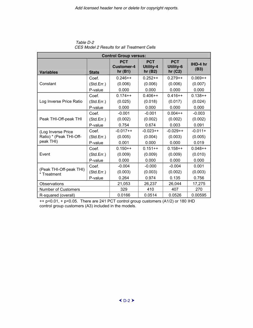
Add licensed header here or delete for copyright reports.
D-2
Table D-2 CES Model 2 Results for all Treatment Cells
Control Group versus:
Variables Stats
PCT Customer-4
hr (B1)
PCT Utility-4 hr (B2)
PCT Utility-6 hr (C2)
IHD-4 hr (B3)
Constant Coef. 0.246++ 0.252++ 0.279++ 0.069++ (Std.Err.) (0.006) (0.006) (0.006) (0.007) P-value 0.000 0.000 0.000 0.000
Log Inverse Price Ratio Coef. 0.174++ 0.406++ 0.416++ 0.138++ (Std.Err.) (0.025) (0.018) (0.017) (0.024) P-value 0.000 0.000 0.000 0.000
Peak THI-Off-peak THI Coef. -0.001 -0.001 0.004++ -0.003 (Std.Err.) (0.002) (0.002) (0.002) (0.002) P-value 0.754 0.674 0.003 0.091
(Log Inverse Price Ratio) * (Peak THI-Off-peak THI)
Coef. -0.017++ -0.023++ -0.029++ -0.011+ (Std.Err.) (0.005) (0.004) (0.003) (0.005) P-value 0.001 0.000 0.000 0.019
Event Coef. 0.150++ 0.151++ 0.158++ 0.048++ (Std.Err.) (0.009) (0.009) (0.009) (0.010) P-value 0.000 0.000 0.000 0.000
(Peak THI-Off-peak THI) * Treatment
Coef. -0.004 -0.000 -0.004 0.001 (Std.Err.) (0.003) (0.003) (0.002) (0.003) P-value 0.264 0.974 0.135 0.756
Observations 21,053 26,237 26,044 17,275 Number of Customers 329 410 407 270 R-squared (overall) 0.0166 0.0514 0.0526 0.00595 ++ p<0.01, + p<0.05. There are 241 PCT control group customers (A1/2) or 180 IHD control group customers (A3) included in the models.

D-3
Table D-3 Demand Elasticity Results Log-Linear Models
Control Group versus:
Variables Stats
PCT Customer-4 hr (B1)
PCT Utility-4 hr (B2)
PCT Utility-6 hr (C2)
IHD-4 hr (B3)
Log Average Price Coef. -3.870++ -3.684++ -3.685++ -1.578++ (Std.Err.) (0.043) (0.035) (0.031) (0.043) P-value 0.000 0.000 0.000 0.000
Average THI Coef. -0.033 -0.018 -0.026 -0.039 (Std.Err.) (0.026) (0.020) (0.015) (0.024) P-value 0.194 0.362 0.081 0.111
Event Coef. 0.057++ 0.057++ 0.057++ 0.021++ (Std.Err.) (0.001) (0.001) (0.001) (0.001) P-value 0.000 0.000 0.000 0.000
Avg THI*Treatment Coef. 0.035++ 0.035++ 0.035++ 0.024++ (Std.Err.) (0.007) (0.007) (0.007) (0.008) P-value 0.000 0.000 0.000 0.002
Constant Coef. 0.001 -0.004++ -0.004++ -0.001 (Std.Err.) (0.002) (0.001) (0.001) (0.002) P-value 0.628 0.002 0.001 0.717
Observations 21,055 26,240 26,047 17,278 Number of Customers 329 410 407 270 R-squared (overall) 0.147 0.116 0.107 0.0170 ++ p<0.01, + p<0.05. There are 241 PCT control group customers (A1/2) or 180 IHD control group customers (A3) included in the models.

Add licensed header here or delete for copyright reports.
D-4
Table D-4 Demand Elasticity Model 2 Results for all Treatment Cells
Control Group versus: Variables Stats PCT
Customer-4 hr (B1)
PCT Utility-4 hr (B2)
PCT Utility-6 hr (C2)
IHD-4 hr (B3)
Log Average Price Coef. -5.990++ -4.302++ -4.161++ -3.887++ (Std.Err.) (0.569) (0.402) (0.297) (0.528) P-value 0.000 0.000 0.000 0.000
Average THI Coef. -0.934+ -0.282 -0.230 -1.021+ (Std.Err.) (0.448) (0.317) (0.238) (0.406) P-value 0.037 0.374 0.333 0.012
Event Coef. 0.086++ 0.065++ 0.063++ 0.052++ (Std.Err.) (0.014) (0.010) (0.008) (0.013) P-value 0.000 0.000 0.000 0.000
Avg THI*Treatment Coef. 0.035++ 0.035++ 0.035++ 0.024++ (Std.Err.) (0.007) (0.007) (0.007) (0.008) P-value 0.000 0.000 0.000 0.002
(Log Average Price) * (Average THI)
Coef. -0.000 -0.004++ -0.005++ -0.002 (Std.Err.) (0.002) (0.001) (0.001) (0.002) P-value 0.957 0.002 0.001 0.340
Constant Coef. 0.012+ 0.004 0.003 0.013+ (Std.Err.) (0.006) (0.004) (0.003) (0.005) P-value 0.044 0.405 0.390 0.015
Observations 21,055 26,240 26,047 17,278 Number of Customers 329 410 407 270 R-squared (overall) 0.151 0.113 0.104 0.00967 ++ p<0.01, + p<0.05. There are 241 PCT control group customers (A1/2) or 180 IHD control group customers (A3) included in the models.

E-1
Appendix E: Sample Frame Customer Demographics
The graphics below display the survey responses from customer that completed the survey FirstEnergy to establish the sampling frame for the CBS.
Figure E-1 Home Size
0%
5%
10%
15%
20%
25%
30%
35%
40%
45%
50%
Control Group -IHD
IHD 4 Hr None Control Group -PCT
PCT FE Control 4 Hr
PCT FE Control 6 Hr
PCT Self Control 4 Hr
None
Non-CAC CAC
Perc
ent R
espo
nden
ts
Home Size
<1000 Sq Ft 1000-1499 Sq Ft 1500-1999 Sq Ft 2000-2999 Sq Ft >=3000 Sq Ft [blank]

Add licensed header here or delete for copyright reports.
E-2
Figure E-2 Type of Home
0%
10%
20%
30%
40%
50%
60%
70%
80%
90%
100%
Control Group -IHD
IHD 4 Hr None Control Group -PCT
PCT FE Control 4 Hr
PCT FE Control 6 Hr
PCT Self Control 4 Hr
None
Non-CAC CAC
Perc
ent R
espo
nden
ts
Type of Home
Single Family Home Duplex or Two-Family Home Condominium Mobile Home Other [blank]
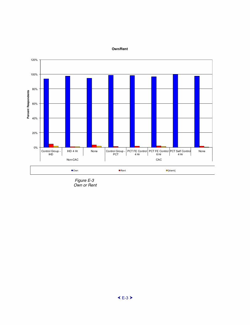
E-3
Figure E-3 Own or Rent
0%
20%
40%
60%
80%
100%
120%
Control Group -IHD
IHD 4 Hr None Control Group -PCT
PCT FE Control 4 Hr
PCT FE Control 6 Hr
PCT Self Control 4 Hr
None
Non-CAC CAC
Perc
ent R
espo
nden
ts
Own/Rent
Own Rent [blank]

Add licensed header here or delete for copyright reports.
E-4
Figure E-4 Education Level
0%
5%
10%
15%
20%
25%
30%
35%
40%
Control Group -IHD
IHD 4 Hr None Control Group -PCT
PCT FE Control 4 Hr
PCT FE Control 6 Hr
PCT Self Control 4 Hr
None
Non-CAC CAC
Perc
ent R
espo
nden
ts
Highest Level of Education
Elementary School or Less Some High School Graduated High School or Equivalent Trade School after High School
Some College Graduated College Post-Graduate Degree [blank]

E-5
Figure E-5 Income Level
0%
5%
10%
15%
20%
25%
30%
Control Group -IHD
IHD 4 Hr None Control Group -PCT
PCT FE Control 4 Hr
PCT FE Control 6 Hr
PCT Self Control 4 Hr
None
Non-CAC CAC
Perc
ent R
espo
nden
ts
Income level
<$15,000 >=$15,000 and <$25,000 >=$25,000 and <$35,000 >=$35,000 and <$50,000 >=$50,000 and <$75,000
>=$75,000 and <$100,000 >=$100K and <$150K >=$150K and <$200K >=$200K [blank]