TSTE91 System Design

Communications System Simulation Using Simulink

Part V OFDM by IFFT Modulation

Sebastian Prot, Kent PalmkvistElectronic Systems, Dept. EE, LiTH

020303

2

2

1 Abstract ................................................................................................. 1

2 Theory. .................................................................................................. 1

2.1 OFDM Principle........................................................................... 1

2.2 Fourier Transform....................................................................... 12.2.1 Complex Discrete Fourier Transform ..................................... 22.2.2 The inverse DFT..................................................................... 42.2.3 The Fast Fourier Transform.................................................... 5

2.3 IEEE 802.11a standard (frequency domain frame composition)5

2.4 Sampling vs. signal spectrum....................................................... 6

3 Block descriptions................................................................................. 83.1.1 Transmitter ........................................................................... 10

3.1.1.1 Discrete constant ........................................................... 103.1.1.2 IFFT.............................................................................. 103.1.1.3 Unbuffer........................................................................ 11

3.1.2 Receiver................................................................................ 113.1.2.1 Buffer............................................................................ 113.1.2.2 FFT ............................................................................... 12

3.1.3 Measurement Tools .............................................................. 123.1.3.1 Short-Time FFT ............................................................ 123.1.3.2 Frequency Frame Scope ................................................ 133.1.3.3 Upsample ...................................................................... 13

4 The system basics................................................................................ 13

4.1 The system setup parameters .................................................... 144.1.1 Initial commands .................................................................. 15

4.2 The signals flow .......................................................................... 164.2.1 Measurement section ............................................................ 18

4.3 Transmission analyses................................................................ 184.3.1 The frequency domain frame composition............................ 184.3.2 Received signal spectrum...................................................... 204.3.3 Transmission statistics .......................................................... 21

5 Bibliography: ...................................................................................... 22

1

OFDM by IFFT modulation

1 Abstract

The Matlab/Simulink implementation of the OFDM transmission scheme,performed by IFFT modulation and FFT demodulation, is the main subject ofthis laboratory. Thus, this manual introduces the theory on the Fast FourierTransform, and its application in the carrier modulation process.

2 Theory.

The basic information on the multicarrier transmissions was described inthe other manual introducing multicarrier transmission in basic form –performed by parallel transmitters/receivers.

2.1 OFDM PrincipleOFDM is a special type of multicarrier transmission, where several data

streams modulate different subcarriers. The subchannels spectrum overlap.Figure 1b) presents an OFDM transmission example of three data

substreams with 1/3TB bit rate each. In this example data substreams areproduced by source signal demultiplexation (Fig.1a).

Comparing both FDM and OFDM signal bandwidth an conclusion can bedrawn that the later needs half the bandwidth when the number of channels ismuch larger then one.

2.2 Fourier TransformThe hardware implementation of a multicarrier system, basing on the set of

transmitters and receivers, is impractical because of huge number of elementsneeded. Fortunately, there exist an easy way to modulate a high number ofcarriers and reversing this process using quite simple calculation algorithm andapplying it in DSP architecture.

The discrete fourier transform (DFT) is very well suited for performingmodulation and demodulation using multiple carriers. It contains also an inversetransform called inverse discrete fourier transform (IDFT). The fastimplementation of the discrete fourier transform is called the Fast fouriertransform (FFT).

2

2

Fig.1. a) Single carrier transmission; b) orthogonal frequency divisionmultiplexing with ∆f = 1/(3TB).

If one or more of the terms: DFT, FFT, or IFFT are not known, it isabsolutely necessary to study references and other litterature before continuingwith this manual and attached Simulink model.

2.2.1 Complex Discrete Fourier TransformIf you are already familiar with Fourier transform, you should know that

complex DFT can be viewed as a way of determining the amplitudes and phasesof sine and cosine waves forming an analyzed signal. The equation (1) calledrectangular form of forward complex DFT, explains such signal decompositionfrom a mathematical point of view:

(1) )2sin()2cos(][1

][1

0

−= ∑

−

= N

knj

N

knnx

NkX

N

n

ππ ,

where the X[k] array stores N amplitudes of component frequencies, x[n]array stores N samples of the time domain signal.

The kn/N signifies the frequency of the cosine/sine wave (for each k∈[0,N-1], n varies between 0 and the total number of time domain samples). Theparameter k defines the number of complete cycles of sine/cosine wave that

3

3

occur over the N points of the time domain signal stored in the x[n] array. Theparameter n signifies the number of collected time domain sample.

Since (1) defines a complex Fourier transform, both: the time domain andthe frequency domain array store complex values.

The X[k] array includes both: positive and negative frequencies, where anindex between k=0 and k=N/2 defines positive frequencies, and an indexbetween k=N/2+1 and k=N-1 defines negative frequencies (Fig.2).

There are two main ways of applying complex DFT in electronic systems:• the time domain signal is assumed to be totally real,

o the real part of frequency domain signal has an even symmetry andimaginary part has an odd symmetry (fig.3);

• the time domain is assumed to be complex:o positive and negative frequencies are independent of eachother.

The system of totally real time domain signal is for e.g., applied in ADSL(Asynchronous Digital Subscriber Line) technology, and will not be discussed inthis manual.

The second above mentioned system is recommended by 802.11a IEEEStandard in W-LAN (Wireless LAN) applications.

The last thing to note about the DFT is the frequency distance between eachsample in the frequency domain (the resolution). It depends on the samplingfrequency fS and FFT length N (2):

(2) N

fF S=∆

4

4

Fig.2. Graphic presentation of complex forward and inverse DFT algorithm.Dashed lines represent the forward DFT, and solid lines visualize inverse

discrete Fourier transform. The frequency array consists of positive and negativefrequencies. The positive frequencies run from 0 to N/2.

Fig.3. The example of the complex spectrumrepresenting an entirely real time domain signal.

2.2.2 The inverse DFTThe forward DFT decomposes signals into several component sinusoids,

equally spaced in the particular frequency range.On the other hand, the inverse DFT summarizes all sine and cosine waves

of amplitudes stored in X[k] array, to form again the time domain signal to betransmitted, as presented in figure 2 and as calculated in (3).

(3). )2sin()2cos(][][1

0∑

−

=

+=

N

k N

knj

N

knkXnx ππ

(4). ][Im][Re][ kXjkXkX +=

Putting (4) into (3):

5

5

( )

∑

∑

∑

∑

∑

−

=

−

=

−

=

−

=

−

=

++

+

−=

=

−+

+

+=

=

++=

1

0

1

0

1

0

1

0

1

0

)2sin(][Re)2cos(][Im

)2sin(][Im)2cos(][Re

)2sin(][Im)2cos(][Im

)2sin(][Re)2cos(][Re

)2sin()2cos(][Im][Re][

N

k

N

k

N

k

N

k

N

k

nN

kkXn

N

kkXj

N

knkX

N

knkX

N

knkX

N

knkXj

N

knkXj

N

knkX

N

knj

N

knkXjkXnx

ππ

ππ

ππ

ππ

ππ

Substituting X[k] in (3) for ReX[k]+j ImX[k] and carrying out thecalculations, an conclusion can be drawn that:

• each value of the real part in the frequency domain contributes to thetime domain:

o real cosine and imaginary sine wave, and• each value of the imaginary part in the frequency domain contributes

to the time domain:o real sine and imaginary cosine wave.

In other words, each frequency domain value produces both the realsinusoid and the imaginary sinusoid in the time domain.

Adding all those signals reconstructs the output wave.Cosine and sine waves in (1) and (3) can be understood as real signals

generated by the physical circuits

2.2.3 The Fast Fourier TransformThe direct calculation of the Discrete Fourier Transform is for large sizes of

N very time consuming. The computation time required grows as N2. There ishowever a much more efficient way to calculate the DFT, called the Fast FourierTransform (chapter 12, [1]).

2.3 IEEE 802.11a standard (frequency domain frame composition)The IEEE802.11a standard recommends that a 64 points inverse Fourier

transform should be applied in the process of carriers modulation. Thedifference between the theory introduced in the previous chapters and itspractical implementation is slight but very important.

Reading the theoretical considerations in the chapter 2.2.2, a conclusioncould be drawn that in OFDM transmission system all 64 carriers could be usedfor data transmission. This is not correct!

The justification of this misunderstanding lies in the theoretical vs. practicalboundaries conflict.

6

6

There is nothing to say about transmitting with use of all of the 64 carriersmodulated by applying the IFFT. But, the problems are encountered when itcomes to the signal reception.

According to Nyquist sampling theorem, the signal can be properlysampled, only if it does not contain frequencies above one-half of the samplingrate. If such requirement would not be fulfilled, frequency domain aliasingwould occur (ch.3 of [1]).

Thus, it is necessary to filter the part of the signal spectrum that coulddestroy the information after aliasing (all frequencies above 0,5Fs). Suchfiltering is performed using an analog filter (anitialias filter).

Antialias filter is a low-pass circuit designed to block all frequencies abovethe cutoff frequency, while passing all frequencies below. The key parameters ofsuch circuit are: the stopband attenuation and of course the filter roll-off.

The best circuits offer roll-off of about 0,1 of sampling frequency, andhundreds of decibels of stopband attenuation, what is of course far from ideal.

The consequences are obvious: the frequency band between about 0,4 and0,5 of the sampling rate is simply a wasted resource due to the filters slow roll-off and non ideal stopband attenuation.

Taking all into consideration, the frequency frame samples definingamplitudes of signals between 0,4 and 0,5 of the sampling rate are not totransmit any data since it would be lost anyway. Thus, the 802.11a standardrecommends only 521 of 64 carriers to be used for data transmission.

The other case is the DC component, which according to 802.11a is not tobe used either to avoid the degradation from carrier leakage or a DC offsetcaused by the analog circuits.

2.4 Sampling vs. signal spectrumFrom sampling theory, the analog to digital conversion can be performed by

signal multiplication by the sequence of delta impulses called unity amplitudeimpulse train (fig.4). The resulting digital signal forms an impulse train.Although in practice, it is difficult to achieve enough narrow delta signals.Instead, ADCs (Analog to Digital Converters) hold the last value until the nextsample is received. This process is called zero-order hold. There exist a wholefamily of such signal conversions e.g., first-order hold uses strait lines betweenthe points, second-order hold uses parabolas etc.

As was mentioned in the previous manual, the discrete signal in one domainis cyclic in the other. Additionally, even if the original time domain signal isinfinite in length, it needs to be cut into finite frames. Each frame is consideredto be a single period (of an infinitely periodic signal) of the input DFT signal.

1 Cumulated around the DC component.

7

7

Fig.4. The sampling theory. The time domain signal multiplicationcorresponds with the frequency domain convolution. Fs=1/T.

Thus, both sampling methods: with impulse train2 and zero-order hold,generate cyclic but not identical spectrums. The frequency spectrum of unityimpulse train is also a unity amplitude impulse train, with the spikes occurring atmultiples of the sampling frequency, fs, 2fs, 3fs, 4fs, etc., (fig.4). Since the timedomain signal is a multiplication of the data and the impulse train, in thefrequency domain – due to the convolution – original spectrum is copied to thelocation of each spike in the impulse train spectrum.

In the stairs signal case, the spectrum is additionally multiplied by the sincfunction (5).

2 Unity amplitude impulse train

8

8

(5). )sin(

)(S

S

ff

ff

fH π

π

=

Equation (5) describes high frequency amplitude reduction due to the zero-order hold. The sampling frequency represents fs. For f=0 H(f)=1 (fig.5).

Fig.5. The comparison of the impulse train and zero-order hold sampled signalspectrum.

3 Block descriptions

The Simulink model presents a simplified OFDM transmission system,which introduces the application of the IFFT/FFT elements in the process ofdata modulation/demodulation according to the IEEE802.11a standard.

In the same way as the other simulink models in this course, the system wasdivided into three basic sections (fig.7):

• Transmitter,• Receiver, and• Measurement Tools.

9

Fig.7. The system introducing the OFDM transmission by IFFT modulation and FFT demodulation.

10

All of above mentioned sections introduce some new blocks, listed below:• FFT,• IFFT,• Buffer,• Unbuffer,• Discrete constant,• Baseband S-QASK demod,• Frequency Frame Scope,• Short-Time FFT,• Upsample.

3.1.1 Transmitter

3.1.1.1 Discrete constantDiscrete constant block is applied in this model to generate the zeroed

samples, which are further converted to complex form (fig.6). Zeros areincluded in the frequency frame to be converted to the time domain signal andtransmitted over the channel.

Fig.6. The discrete constant block dialog box (on the left) and Real-Imag tocomplex block in single subsystem(on the right).

3.1.1.2 IFFTThe IFFT block (fig.8) computes the Inverse Fast Fourier Transform of

each Y complex input channels. The block assumes that the input is an X-by-Yframe matrix and that each of the Y frames contains X sequential time samplesfrom an independent signal.

11

11

Fig.8. IFFT block dialog box.

3.1.1.3 UnbufferUnbuffer block is used in the system as parallel to serial converter (fig.9).

Fig.9. The Unbuffer block dialog box.

3.1.2 Receiver

3.1.2.1 BufferThe buffer block is used as serial to parallel converter in this system. It fills

each buffer with 64 samples incoming form the channel and passes the frame tofarther processing. The number of samples forming the time domain frame isdetermined by the 802.11a IEEE standard.

The block introduces a nonzero latency, which can be calculated by typingthe command rebuffer_delay(f,n,m) in the Matlab command window, wheref defines the input frame size – in this case 1, n is the Buffer size (fig.10)parameter setting – in this case 64, and m is the Buffer overlap parameter settingwhich in this case is 0. When executed, this command returns 64 – single, fullbuffer latency (frame size).

12

12

Fig.10. Buffer block dialog box.

3.1.2.2 FFTThe FFT block computes the fast Fourier transform (FFT) of each input

frame, independently at each sample time (fig.11). Each input frame is called achannel in the Simulink environment.

Fig.11. FFT block dialog box.

3.1.3 Measurement Tools

3.1.3.1 Short-Time FFTFrom Matlab help file: “The block averages the squared magnitude of the

FFT computed over windowed sections of the input, and normalizes the spectralaverage by the square of the sum of the window samples”.

The window function that shapes the input impulses can be set to any fromsupplied list (fig.12).

Block dialog box allows setting several parameters. The most important are:• FFT length,• Number of spectral averages,

FFT lengthThe received signal is first buffered. Each frame consists of 256 time

domain samples, thus includes four OFDM symbols. Since the input frame doesnot need to be zero padded, the frame size can be inherited from input frame

13

13

width. Input frame size was determined experimentally, so the center frequencycould be clearly identified as the not modulated part of signal spectrum.

Fig.12. ST-FFT model dialog box on the left.Spectrum Calculation Subsystem, on the right.

Number of spectral averagesThe higher value the more smooth spectrum envelope is presented on the

Frequency Frame Scope. However, more averages needs more computationtime, and more memory to be used by the system.

The value of this parameter was also determined experimentally so thespectrum does not include to many peak values, and SNR parameter change,effects in relatively fast plotted spectrum updating.

3.1.3.2 Frequency Frame ScopeThis block allows the user to present the generated frequency frame, e.g., by

the power spectrum calculation systems. The input frame parameters areidentical to those described in chapter 2.3. The model dialog box is similar toalready known FFT Frame Scope, and does not need any further explanation.

3.1.3.3 UpsampleThe Upsample block resamples the discrete input at a rate L times higher

than the input sample rate by inserting L-1 zeros between consecutive inputsamples.

4 The system basicsBefore starting the simulation, you should first analyze the system carefully

and try to understand dependencies between particular blocks, parameters, etc.

14

14

The following description explains the signals flow and tasks that arerealized by different system stages.

4.1 The system setup parametersBefore starting the simulation, it is necessary to set basic transmission

parameters (fig.13):• M-ary data mapping,• Signal to Noise Ratio in the transmission channel.

Fig.13. The system setup dialog box.

M-ary data mappingThe IFFT block accepts only complex signals on its input. Thus, the M-ary

real signal needs to be converted to complex form. Such conversion is nothingmore but simple baseband complex data mapping.

According to IEEE 802.11a standard - ch.17.3.5.7, one of four gray-codedQASK maps (table.1) should be applied for OFDM transmission. In theSimulink environment can the Square-map QASK modulator be used for thispurposes.

The parameter M can be altered while the simulation is running.

Baseband mapping modes recommended byTable 1. IEEE 802.11a standard for OFDM transmission.

M Mapping Mode2 BPSK4 QPSK16 16-QAM64 64-QAM

15

15

SNR in the transmission channelTo achieve error free transmission in OFDM, the SNR needs to be higher

than 20 dB. The higher M value the higher SNR parameter value needed toachieve error free transmission.

This parameter can also be altered while the simulation is running.

4.1.1 Initial commands

To prepare the system for optional future development and to visualizesome system dependencies, all the basic transmission parameters (table.2) arecollected in the initial commands section of the system mask editor (fig.14).

Fig.14. Mask editor with initial commands defined.

Table.2. System initial commands

%Subcarriers related parameters according to ch.17.3.2.3 of IEEE Std802.11a%----------------------------------------Nsd=48; % Number of data subcarriersNsp= 4; % Number of pilot subcarriersNst =Nsd+Nsp; % Number of subcarriers, total (52)%------------------------------------------------------------------------------------------% Parameters of names not following Std802.11a labeling%----------------------------------------BW=20e6; %Cumulative signal bandwidth (20Msamples/s)ChTSamp=1/BW; % The time duration between samples in the channelSubchannelBW=BW/64; %Subchannels signal bandwidthTbit=1/SubchannelBW; %Subchannel signal sample time

16

16

4.2 The signals flowThe IEEE 802.11a standard defines 52 total subchannels over which data is

to be transmitted. This includes 4 subchannels used for pilot signal transmission.According to the mentioned standard, pilots are to be BPSK mapped andmodulated by special pseudorandom sequences.

Notice, that for simplification this model does not distinguish between dataand pilots signals. Thus, the data source generates 52 M-ary simultaneous datastreams (fig.15). Each substream is further mapped to complex form with use ofone of 52 QASK baseband modulators (fig.16).

Fig.15. The data source generates cyclically repeatable 1000 frames of M-arysymbols. Each frame is Nst=52 samples wide, which corresponds to

52 simultaneous data substreams.

Fig.16. The QAM baseband modulators set.

17

17

The stream of complex numbers is divided into 2 groups of 26 samples.One of them becomes negative frequency magnitudes, and the other positivefrequency magnitudes (fig.17).

To avoid difficulties in D/A and A/D converter or offsets and carrierfeedthrough in the RF systems, the 0-th subcarrier (DC frequency) is not used –all transmitted samples are zeroed.

Since this system models baseband transmission, these mentioned problemswould not occur anyway. The model still follows the standard recommendation.

Fig.17. The frequency frame formation section.

Fig.18. The redundant samples discarding section.

18

18

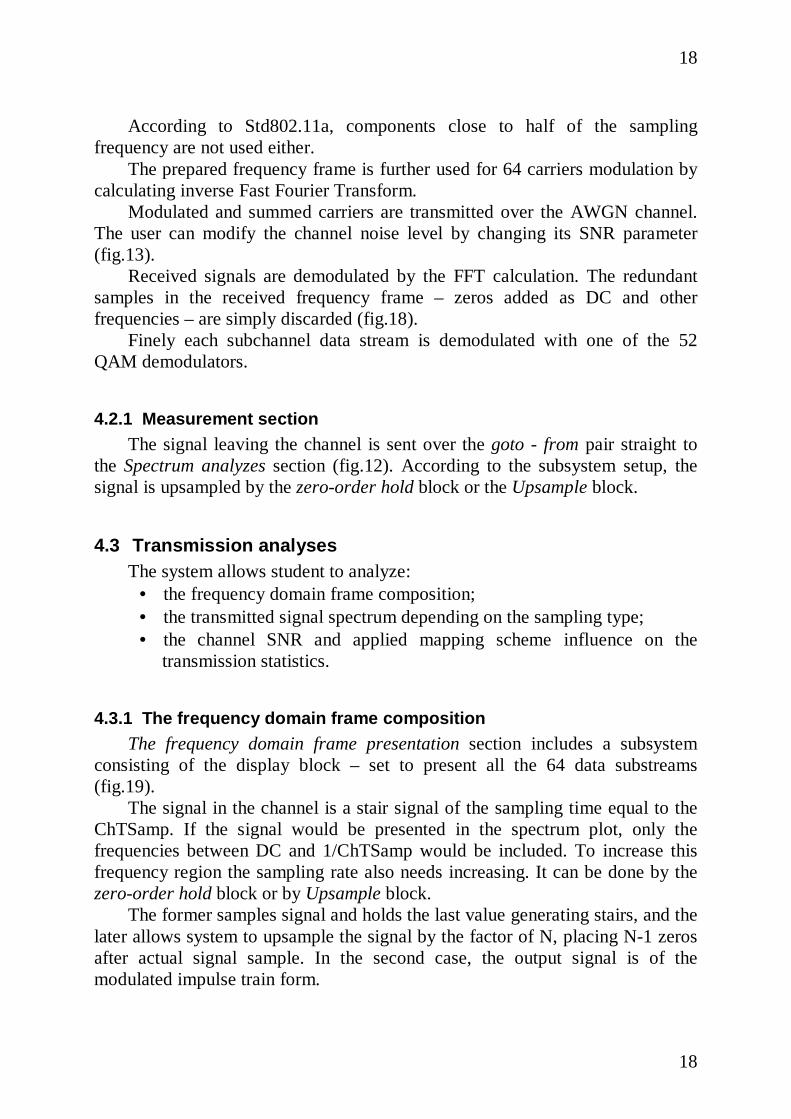
According to Std802.11a, components close to half of the samplingfrequency are not used either.

The prepared frequency frame is further used for 64 carriers modulation bycalculating inverse Fast Fourier Transform.

Modulated and summed carriers are transmitted over the AWGN channel.The user can modify the channel noise level by changing its SNR parameter(fig.13).

Received signals are demodulated by the FFT calculation. The redundantsamples in the received frequency frame – zeros added as DC and otherfrequencies – are simply discarded (fig.18).

Finely each subchannel data stream is demodulated with one of the 52QAM demodulators.

4.2.1 Measurement sectionThe signal leaving the channel is sent over the goto - from pair straight to

the Spectrum analyzes section (fig.12). According to the subsystem setup, thesignal is upsampled by the zero-order hold block or the Upsample block.

4.3 Transmission analysesThe system allows student to analyze:

• the frequency domain frame composition;• the transmitted signal spectrum depending on the sampling type;• the channel SNR and applied mapping scheme influence on the

transmission statistics.

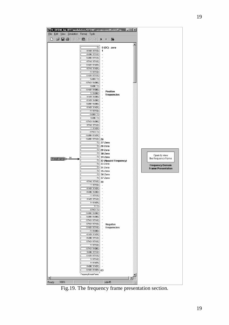
4.3.1 The frequency domain frame compositionThe frequency domain frame presentation section includes a subsystem

consisting of the display block – set to present all the 64 data substreams(fig.19).

The signal in the channel is a stair signal of the sampling time equal to theChTSamp. If the signal would be presented in the spectrum plot, only thefrequencies between DC and 1/ChTSamp would be included. To increase thisfrequency region the sampling rate also needs increasing. It can be done by thezero-order hold block or by Upsample block.

The former samples signal and holds the last value generating stairs, and thelater allows system to upsample the signal by the factor of N, placing N-1 zerosafter actual signal sample. In the second case, the output signal is of themodulated impulse train form.

19

19

Fig.19. The frequency frame presentation section.

20

20

4.3.2 Received signal spectrumThe spectrum analysis section allows student to compare the discrete signal

spectrum depending on the applied sampling type, which can be set in thesubsystem dialog box (fig.20).

Fig.20. The spectrum analysis section dialog box.

The frequency frame scope presents the calculated signal spectrumdepending on the sampling type selection. Notice, that before changing thisparameter simulation needs to be stopped.

Fig.21. The OFDM signal spectrum (stairs signal).

The stairs signal spectrum is influenced by the high frequencies attenuation(fig.21, ch.2.1), while the spectrum of tje modulated impulse train signal isperiodic in the whole analyzed frequency band (fig.22). High frequenciesattenuation of the stairs spectrum can be modeled as spectrum multiplication bythe sinc function (5).

The channel SNR parameter influence on the signal spectrum can also beanalyzed with the use of the frequency frame scope. When changing the SNRparameter below 20dB, the noise level can be observed in the regionsrepresenting not modulated frequencies (fig.23).

21

21

Fig.22. The OFDM signal spectrum (modulated impulse train).

Fig.23. The noise level related to the mean signal level.

4.3.3 Transmission statisticsThe display block presents the Symbol Error Rate (fig.24).

Fig.24. SER presentation section.

22

22

5 Bibliography:

[1]. “The Scientist and Engineer's Guide to Digital Signal Processing”, Steven W. Smith.