using tdr technology for earthwork compaction quality …

Using TDR Technology for Earthwork Compaction Quality Control

Presentation to the California Geotechnical Engineers Association January 15, Orange County, CA

January 22, Sacramento, CA

Presented by Gary N. Durham, Ph. D., P.E., President

Durham Geo Slope Indicator Licensed Technology In November 2003, we entered into a license agreement with Purdue University for the rights to commercialize, manufacturer and distribute the Purdue TDR Method for measuring water content and density of soil. In the ensuing year we engaged in product design to transform the research prototype into a commercially viable product. This month we began introducing the product to our customers. The new technology has been under development at the CE Department of Purdue University for the past ten or so years under the direction of Dr. Vincent Drnevich. Several patents have been issued for various parts of the research. Acknowledgements The following is a summary of the TDR technology to measure water contents and densities of compacted earth fill. In developing this presentation I have borrowed liberally from the published research of Purdue and list some of the more pertinent papers and publications at the end for those who wish to gain further insight into the research. Time domain reflectometry (TDR) was developed in the 1930s to locate breaks in coaxial cables. TDR has been compared to wire radar. When a policeman uses a radar gun to clock your car’s speed, the signal travels from the gun to your car, bounces of the car and part of the energy reflects back to a receiver in the gun.

In a TDR system, a pulse generator injects a fast-rising voltage pulse into a coaxial cable. The pulse travels the length of the cable, bounces off the far end (or at a break or crimp), and returns through the cable. The entire process can be viewed on an oscilloscope or individual data points displayed on a PC. Signals travel through cables at a percentage of the speed of light. The inside insulator of a coaxial cable determines how quickly a signal propagates and that is a function of the dielectric properties of the insulator. This brings us to dielectric constant which is the ratio squared of the propagation velocity in vacuum relative to that in the medium.

K = (c/v)2 (1) where K – Dielectric constant

c – Velocity of electromagnetic waves in vacuum (3 x 108 m/s) v – Velocity of electromagnetic wave in medium

The dielectric constant for air is about 1, water about 81 and soil minerals 3 to 5. Since the 1980s soil scientists have engaged in research by a three prong probe and TDR to determine the volumetric water content of soil. Much of this early research formed the basis for Purdue’s work. Purdue’s Technology The Purdue TDR system (see Figure 1) consists of the following:

• TDR device • Coaxial cable

Figure 1: TDR System

• Coaxial head • Either a coaxial cylinder or

multiple probe arrangement • Portable computer interface

such as a PC notebook or PDA

The field carrying case for these components is shown in Figure 2.

Figure 2: Field Carrying Case for TDR Components

A spike is inserted into the ground to simulate the coaxial cable’s conductor and the cable’s shielding is modeled with three equally spaced spikes around the circumference of a 4-in diameter circle as shown in Figure 3(a). The “soil cable” is completed by placing the coaxial head on the four probes (Figure 3(b)). The in-situ soil represents the insulator.

Figure 3(a): Spikes Driven in the Soil. The Template PPrecise Positioning.

rovides Figure 3(b): Coaxial Head Positioned on Top of the Four Spikes (probes).

In the laboratory, Figure 4, we use a 4-in diameter compaction mold mounted on a non-conductive base with a center probe such that the mold’s wall models the shielding. The TDR pulse generator sends out a step pulse of 0.25 volts that lasts 14 microseconds. It travels down the coaxial cable to a specially designed probe that simulates a coaxial cable where the insulating medium is soil. The rise time of the voltage must be very fast, typically on the order of 200 picoseconds. The rise time of the voltage along with the reflected voltage is monitored as a function of time. A typical signal for a TDR test on soil is shown in Figure 5 where voltage is plotted versus “apparent distance” in meters, which is defined as the wave travel time multiplied by the speed of light in a vacuum and divided by two. Referring to Figure 5, as the signal reaches the head assembly, a reflection takes place as indicated by a voltage increase (1-1). After passing through the head assembly, another reflection occurs due to the impedance mismatch of the air/material interface (2-2), which causes an abrupt voltage drop in the TDR signal. This results in the first peak of the TDR signal. Following the reflection, voltage continues to decrease until the wave front encounters another impedance mismatch when the signal reaches the tapered end of the probe, another reflected signal (3-3).

Figure 4: (L) Center Probe Driven into a 4-inch Mold with a Guide Ring. (R) Coaxial Head Placed on Top of the 4 inch Mold.

(a)

(b) Typical waveforms for various soil types are illustrated in Figure 6. The voltage travels through the soil at a velocity that is proportional to the apparent dielectric constant, Ka of the soil. Referring to Figure 7, the distance between the first peak and the rebound is proportional to the time of wave travel over the length of the “soil cable.” Figure 5: TDR System Schematic: a) Reflections in

the TDR System; and b) Resulting TDR Waveform.

-1.5

-1

-0.5

0

0.5

1

1.5

-0.5 0.5 1.5 2.5 3.5 4.5 5.5 6.5 7.5

Distance (m)

Am

plitu

deOTTAWA SAND

ML SILT

CL CLAY

TDR Results

Figure 6: Typical Waveforms for Various Soil Types

Figure 7: Typical TDR Waveform for Soil Showing Measurements to Obtain Apparent Dielectric Constant, Ka.

The apparent dielectric constant is calculated from:

2

⎟⎟⎠

⎞⎜⎜⎝

⎛=

p

aa L

LK

Where La = length of the “soil cable” and Lp = probe length.

(2)

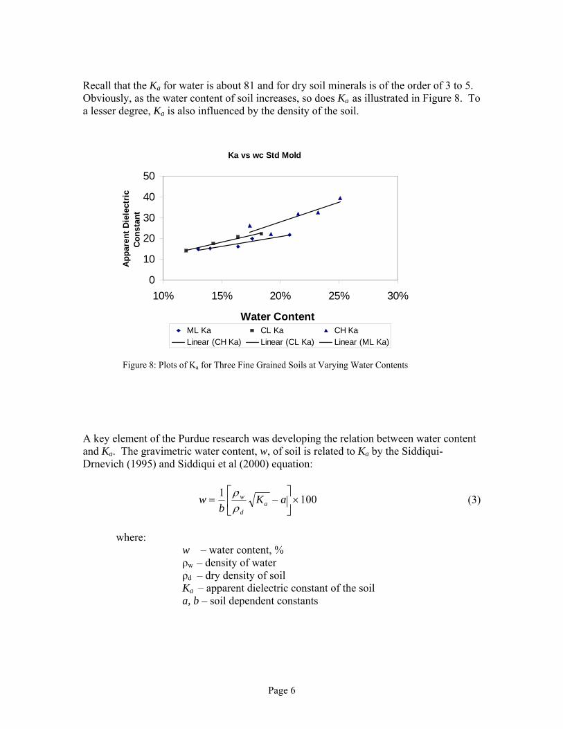
Recall that the Ka for water is about 81 and for dry soil minerals is of the order of 3 to 5.

key element of the Purdue research was developing the relation between water content

Obviously, as the water content of soil increases, so does Ka as illustrated in Figure 8. Toa lesser degree, Ka is also influenced by the density of the soil.

Ka vs wc Std Mold

0

10

20

30

40

50

10% 15% 20% 25% 30%

Water Content

App

aren

t Die

lect

ric

Con

stan

t

ML Ka CL Ka CH KaLinear (CH Ka) Linear (CL Ka) Linear (ML Ka)

Figure 8: Plots of Ka for Three Fine Grained Soils at Varying Water Contents

Aand Ka. The gravimetric water content, w, of soil is related to Ka by the Siddiqui-Drnevich (1995) and Siddiqui et al (2000) equation:

1001×⎥

⎦

⎤⎢⎣

⎡−= aK

bw a

d

w

ρρ (3)

where:

w – water content, %

l constant of the soil

ρw – density of water ρd – dry density of soiKa – apparent dielectric a, b – soil dependent constants

The values of a and b vary with soil type with the value of a approximately equal to 1 and b between 8 and 9 (Table 1). However, for a given soil, unique values of a and b are obtained by compacting several soil samples with like compaction energy but at varying water contents in a mold and determine the Ka for each compaction point. The “soil cable” is the probe inserted (see Figure 9 (a)) in the center of the mold (conductor) and the mold forms the shield (see Figure 9 (b)).

(a) (b)

Figure 9: (a) Installation the Center Rod; (b) Adapter Ring and Probe Head Installed.

Table 1 - Typical Values of Soil Constants a and b

USCS Soil

constants Soil Description Region Symbol a b

Ottawa Sand Illinois SP 1.03 7.83 Sandy Soil Florida SP 1 8.45 Brown County Clay Ohio CL 0.91 8.84 Glacial Till Indiana SM 1.02 9.06 Loess Mississippi ML 1.21 7.95 Lean clay Mississippi CL 1.3 7.93 Buckshot clay Mississippi CH 1.22 10.97

Determining In-situ Water Content and Density by the TDR Method Two methods have resulted from the Purdue research programs. The first method developed is referred to as the Two-Step Method but subsequent development resulted in the Simplified or One-Step Method. Key points of the two methods are:

Two-Step Method (see Figure 10) • In-situ TDR measurement made • Soil from in-situ test is tamped into a field mold • Wet density of soil in field mold is determined • TDR measurement of field mold is made • Use assumed or determined a and b soil constants to calculate in-situ

water content and dry density

Template for Positioning Probes Probes in Ground (Template Removed) TDR Measurement in-situ

Remove Material from Test Area Compact Soil in TDR Mold Determine Wet Density

TDR Measurement in Mold TDR Waveform and Results

Figure 10: Sequence of Two-Step Method in the Field

Simplified or One-Step Method (see Figure 11)

• Determine six (6) soil constants by taking TDR readings during the laboratory compaction process using, for example, ASTM D698 Standard.

• In-situ TDR measurement is made • Using the six constants and custom software to determine in-situ water

content and dry density.

Template for Positioning Probes Probes in Ground (Template Removed) TDR Measurement in-situ

TDR Waveforms and Results

Figure 11: Sequence of One-Step Method

• We believe that most users will opt to use the Simplified Method as the laboratory work to develop the soil constants with either method is about the same, but the field effort and time is greatly reduced by eliminating the field mold test of the Two-Step Method. Two-Step Method (ASTM D6780) The Two-Step Method uses either assumed or determined a and b values for a given soil and measured Ka. Recall that the Siddiqui-Drnevich equation has two unknowns — water content and dry density — and a second equation is needed for a closed form solution. That equation is the relation between wet and dry density as:

( )wt

d +=

1ρρ (4)

where: ρt is the total (wet) density of the soil

Solving for ρt in equation 4 and substituting into equation 3 results in

aw

t

w

ta

Kb

aKw

−

−=

ρρ

ρρ

(5)

The Two-Sep Method results in two TDR tests being performed: one to measure (Ka)in-situwhere soil water content and dry density are not known, and one to measure (Ka)mold on the soil excavated from the in-situ location where the total mold density is determined. We modify equation 5 to reflect measurements performed in the mold.

moldaw

moldt

w

moldtmolda

mold

Kb

aKw

,,

,,

−

−=

ρρ

ρρ

(6)

After the in-situ apparent dielectric constant is determined, the soil from the in-situ test location is excavated and tamped into the 4-in diameter by 9-in TDR mold. The compaction energy and resulting density is of little concern as long as the re-compacted material is free of voids and the density is about the same throughout the mold. Our experience has shown that using a standard 5.5-lb sleeve rammer to re-mold the material in six equal layers with each layer receiving 10 blows produces an acceptable sample. The as-compacted density is determined by measuring the mass of the mold and compacted material and using the known volume of the mold. After measuring the mass of the compacted mold, a center probe is driven into the soil, the mold fitted with a special collar and the apparent dielectric constant, Ka,mold, measurement made. Assuming the calibration constants a and b have been determined or can be accurately assigned, all variables on the right side of equation 6 have been measured or are known, and the water content of the mold material can be calculated. If the process of removal of the soil from the in-situ test location and placement into the TDR compaction mold is done quickly, it is valid to assume that the water contents in the mold and at the in-situ location are the same, or

moldsituin ww =− (7)

To determine the constants a and b, the Siddiqui-Drnevich equation can be written in the following form.

bwap

Kd

wa +=ρ (8)

Rewriting equation 8 for in-situ and TDR mold yields

situinbwa −+=situind

wsituina p

K−

−,

,ρ (9)

moldmoldd

wmolda bwa

pK +=

,,

ρ (10)

Assuming water content of the mold is equal to the water content in-situ, the right side of equations 9 and 10 are the same and by substitution

molda

situinamolddsituind K

K

,

,,,

−− = ρρ (11)

The in-situ dry density and water content can be determined through the above sequence. Assuming that soil-dependent constants a and b are known, and with the use of proprietary software, the field procedure will require 15 to 20 minutes. The above process is sensitive to the temperature of the soil and Drnevich et al (2001) provided temperature correction equations. Experience has shown that temperature corrections are not required if soil temperatures at the time of testing are within 20°C ±5°C. Determining a and b soil constants in the laboratory. By examination we see that equation 8 is the basic form of a linear equation and if we plot the left side of the equation against water content, then the y intercept is a and b is the slope. Therefore, the soil-type dependent constants are determined in the laboratory by obtaining a representative sample of the soil undergoing field compaction, divide the sample into four or five test specimen, and adjust the water content of each to cover the range anticipated during field placement. Each test point is compacted in the TDR mold, the apparent dielectric constant measured and the water content determined by oven drying. This sequence of sets is illustrated in Figure 12. Typical waveforms for various molded water contents of a low plastic silt are illustrated in Figure 13.

Soil Preparation Tamping Soil into TDR Mold Weighing the Soil

Apparent Dielectric Constant Measured Ka and ECb are Calculated Extracting the Compacted Sample

Oven Drying Calculating Water Content

Figure 12: Sequence for Determining a and b Soil Constants in the Laboratory

Waveforms for ML Soils

0

0.2

0.4

-0.5 0.5 1.5 2.5 3.5 4.5 5.5 6.5 7.5

Distance (m)

e

-1

-0.8

-0.6

-0.4

-0.2

Am

plitu

d

12.2% w

13.8%w

15.1%w

16.3%w

18.9%w

Figure 13: TDR Waveforms for Silt (ML) at Various Water Contents.

y = 7.8901w.c. + 1.221R2 = 0.8835

0.00

0.50

1.00

1.50

2.00

2.50

3.00

3.50

10.0% 12.0% 14.0% 16.0% 18.0% 20.0% 22.0%

Water Content

aKd

w

ρρ

The data is plotted as illustrated in Figure 14 and the constants a and b determined by best fit of a straight line. Experience to date indicates that the value of a is typically near unity and the value of b is typically around eight to nine.

y 2.31 2.33 2.36 2.63 2.92w.c. 13.0 14.0 16.4 17.6 20.8

l

Figure 14: Plot to Obtain Soil Constants a and b for ML Soi

Simplified (One-Step) Method The Two-Step TDR Method involves two tests in the field, an in-situ Ka measurement and a Ka measurement of in-situ material reconstituted in the TRD mold. Soil-dependent constants are determined in the laboratory or assumed. The Simplified Method does away with the field mold step by incorporating a bulk electrical conductivity measurement and using the individual compaction points of a standard compaction test, such as ASTM D698, for electrical measurements with the TDR device. Bulk Electrical Conductivity – Electrical conductivity is a measure of how well a material accommodates the transport of electric charge. Electrical conductivity is the reciprocal of electrical resistance. Its SI derived unit is the siemens per meter (after Werner von Siemens). It is the ratio of the current to electric field strength. This applies also to the electrolytic conductivity of a fluid. As surface waves propagate along TDR probes buried in soil, the signal energy is attenuated in proportion to the electrical conductivity along the travel path. The bulk electrical conductivity, ECb as defined by TDR waveforms

⎟⎟⎠

⎞⎜⎜⎝

⎛−= 11

f

sb V

VC

EC (12)

where Vs is the source voltage and equal to twice the step voltage, Vf is the long term voltage level (see Figure 15) and C is a constant related to the probe configuration.

⎟⎟⎠

⎞

i

o

sp

dd

RL

⎜⎜⎝

⎛=C

ln

2π (12a)

where Lp is the length of the probe, Rs the internal resistance of the pulse generator, and do and di are outer and inner conductor diameters, respectively (Giese and Tiemann 1975).

Figure 15: Typical TDR Waveform for Soil Showing Measurements to Obtain Apparent Dielectric Constant, Ka, and Bulk D.C. Electrical Conductivity, ECb from the End of a Cable to a Break.

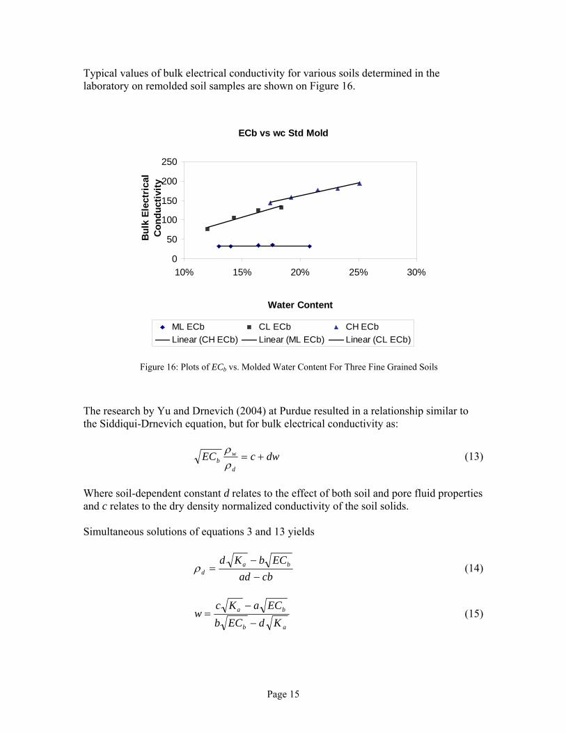
Typical values of bulk electrical conductivity for various soils determined in the laboratory on remolded soil samples are shown on Figure 16.

ECb vs wc Std Mold

0

50

100

150

200

250

10% 15% 20% 25% 30%

Water Content

Bul

k El

ectr

ical

Con

duct

ivity

ML ECb CL ECb CH ECbLinear (CH ECb) Linear (ML ECb) Linear (CL ECb)

Figure 16: Plots of ECb vs. Molded Water Content For Three Fine Grained Soils

The research by Yu and Drnevich (2004) at Purdue resulted in a relationship similar to the Siddiqui-Drnevich equation, but for bulk electrical conductivity as:

dwcd

w +=ECb ρρ (13)

Where soil-dependent constant d relates to the effect of both soil and pore fluid properties and c relates to the dry density normalized conductivity of the soil solids. Simultaneous solutions of equations 3 and 13 yields

cbadECbKd ba

d −−

=ρ (14)

ab

ba

KdECbECaKc

w−

−= (15)

However, the electrical conductivity is sensitive to both temperature and the electrical conductivity of the pore fluid. Hence, water contents and dry densities calculated from equations 14 and 15 generally do not produce satisfactory accuracy primarily due to the differences in pore fluid conductivity between laboratory calibration samples and in-situ samples. The influence of pore fluid on calibration constants for Ka is relatively insignificant; however, the bulk electrical conductivity of laboratory prepared soil using tap water and that of in-situ pore fluid usually differs to varying degrees. Yu and Drnevich (2004) proposed the relationship between the soil apparent dielectric constant, Ka, and the bulk electrical conductivity ECb be expressed as

ab KgfEC +=

situinaadja KK −= ,,

(16) in which f and g are calibration constants related to soil type and pore-fluid conductivity. To relate the ECb,in-situ to the ECb,lab an adjustment is made as follows

(17)

2,, )( situinaadjb KgfEC −+= (18)

Equations 17 and 18 are used in equations 14 and 15 to yield

cbadECbKd adjbadja

d −

−= ,,ρ (19)

adjaadjb

adjb

KdECb ,,

,

−adja ECaKc

w , −= (20)

Temperature effects over the range of temperatures expected in most earth fill placements are very minor as to the Ka but have a greater effect on ECb. Temperature variations from 20°C are adjusted for by taking temperature measurement of the in-situ soil at the time of testing. The Simplified (One-Step) Method for in-situ soil water content and dry density depends on laboratory determination of soil-dependent constants a, b, c, d, f, and g. Laboratory Determination of Soil-Dependent Constants – A benchmark is required to judge the effectiveness of compacting earth fill material and it is compared against the in-situ measurement. The benchmark most often used for non-granular soils is a compaction curve derived by selecting representative soil(s) from the construction

site or borrow area and performing standard laboratory compaction tests such as described in ASTM D698 or ASTM D1557. The soil-dependent constants a, b, c, d, f, and g are obtained in conjunction with performing the laboratory compaction test using constant pore-fluid conductivity such as provided by tap water. The procedure is the same as the one illustrated in Figure 12 (except that a different software program is used) and is summarized as follows:

1. Representative soil is obtained, properly prepared and divided into four or five test specimens with each specimen adjusted to different water content.

2. Following compaction at given water content and the mold plus wet soil mass determined, the mold is placed on a non-conductive base and a central rod driven into the mold using a special guide.

3. An adopted ring is placed on the mold and the legs of the TDR head placed on the ring and the center rod.

4. TDR waveforms are taken from which Ka and ECb are calculated with the assistance of a custom program.

5. The compacted soil is extruded from the mold, oven dried and the water content and dry density calculated.

Steps 2 through 5 are repeated for all the compaction points. The water content, dry density, Ka and ECb for each compaction point are tabulated. Three plots are made of the data:

d

waKρρ1. versus water content

d

wbECρρ versus water content 2.

3. bEC versus Ka A straight line is fitted to the data points of each plot and the respective six constants determined as illustrated in Figure 18. The proprietary computer program mentioned before has a built-in utility to enter the data point, plot the data, calculate the six constants, and places them into the program for use in subsequent field testing. It should be said that the laboratory determination of the six constants can be done after the in-situ testing has been completed as our program has default soil related constants that will produce a tentative field water content and dry density with these tentative field values corrected after the compaction test and TDR measurements are made in the lab.

Soil Preparation Soil Compacted in 4-inch Mold Weighing the Soil

Driving the Center Rod Apparent Dielectric Constant Measured Ka and ECb are Calculated

Extracting the Compacted Sample Oven Drying Calculating Water Content

Figure 17: Sequence for Determining a and b Soil Constants in the Laboratory for the One-Step Method.

(a)

(b)

(c)

Figure 18: Plots for Determining the Six Soil Constants: (a) Ka vs. water content, (b) ECb vs. water content and (c) Ka vs. ECb.

The One-Step Method for determining soil water content and dry density as described above was applied to data obtained from 192 laboratory and field tests. Figure 19 presents water contents determined by the One-Step Method versus water content determined by oven dry water contents. As seen, most of the data points are within ± 1 percentage points of the oven dried value. Figure 20 presents the same set of data for dry density as determined by One-Step Method and the total (wet) density determined by other field methods but converted to dry density using the oven-dried water content value. Results are typically within ± 3 percent. The plotted data represents result from a wide range of soil types and geological settings that include sands, silts, clays, lime and cement stabilized soils, dense graded aggregate base and low density mixed waste.

Special Conditions

Figure 19: Comparison of TDR Water Contents with Oven-Dry Gravimetric Water Contents. (Results are typically accurate to within ±0.01.) 2

Figure 20: Comparison of TDR Dry Density with Dry Density Determined from Total Density (direct measurement, sand cone, or nuclear) with Oven Drying for Water Content. (Results are typically within ± 3%.)2

rocedures

he

Gravelly soils – The TDR method can be used with coarse-textured soils where less than 30 percent by weight of the material has particle sizes exceeding the No. 4 sieve (4.75 mm) and the maximum particle size passes the ¾-inch sieve (19 mm). Most of the research and beta testing performed to date has been conducted on soils with limited gravel permitting the use of 4-in diameter compaction molds and probe placement diameter. Equipment and phave not been fully developed for 6-in diameter molds and probe placement. Nor do we have experience with problems that might be associated with driving tfour probes in heavily compacted aggregates common to base course used in pavements.

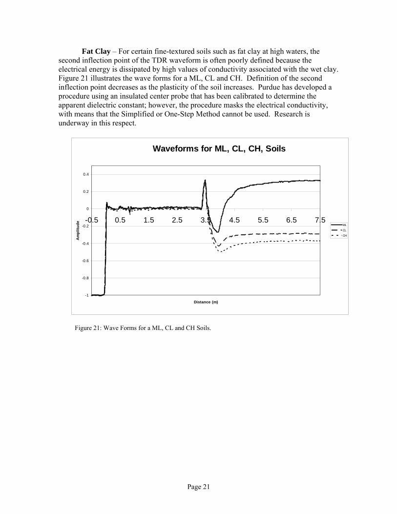
Fat Clay – For certain fine-textured soils such as fat clay at high waters, the second inflection point of the TDR waveform is often poorly defined because the electrical energy is dissipated by high values of conductivity associated with the wet clay. Figure 21 illustrates the wave forms for a ML, CL and CH. Definition of the second inflection point decreases as the plasticity of the soil increases. Purdue has developed a procedure using an insulated center probe that has been calibrated to determine the apparent dielectric constant; however, the procedure masks the electrical conductivity, with means that the Simplified or One-Step Method cannot be used. Research is underway in this respect.

Waveforms for ML, CL, CH, Soils

-1

-0.8

-0.6

-0.4

-0.2

0

0.2

0.4

-0.5 0.5 1.5 2.5 3.5 4.5 5.5 6.5 7.5

Distance (m)

Am

plitu

de ML

CL

CH

Figure 21: Wave Forms for a ML, CL and CH Soils.

References and Suggest Selected Reading 1. Drnevich, V.P., Yu, X., Lovell, J., and Tishmack, J.K. (2001), “Temperature effects

on dielectric constant determined by Time Domain Reflectometry.” TDR 2001: Innovative Applications of TDR Technology, Infrastructure Technology Institute, Northwestern University, Evanston, IL, September, 10 p.

2. Drnevich, V.P., Yu, S., and Lovell, J. (2003), “Beta Testing Implementation of the

Purdue Time Domain Reflectometry (TDR) Method for Soil Water Content and Density Measurement”, Final Report, Report No.: FHWA/IN/JTRP-2000-20, Joint Transportation Research Program, Indiana Department of Transportation – Purdue University, August, 256 p.

3. Giese, K. and Tiemann, R. (1975). “Determination of the complex permittivity from

thin sample time domain reflectometry: Implications for twin rod probes with and without dielectric coatings.” Water Resource Research, Vol. 32 No. 2, 271-279.

4. Siddiqui, S.I. and Drnevich, V.P. (1995), “A new method of measuring density and

moisture content of soil using the technique of Time Domain Reflectometry,” Report No.: FHWA/IN/JTRP-95/9, Joint Transportation Research Program, Indiana Department of Transportation – Purdue University, February, 271 p.

5. Siddiqui, S.I., Drnevich, V.P. and Deschamps, R. J. (2000). “Time domain

reflectometry development for use in geotechnical engineering.” Geotechnical Testing Journal, GTJODJ, Vol. 23, No.1, March, 9-20.

6. Yu, X., and Drnevich, V.P., (2004), “Soil Water Content and Dry Density by Time

Domain Reflectometry,” Journal of Geotechnical and Geoenvironmental Engineering, ASCE, Vol. 130, No. 9, September.

using tdr technology for earthwork compaction quality …

Documents