using principal component analysis (pca) to obtain

USING PRINCIPAL COMPONENT ANALYSIS (PCA) TO OBTAIN AUXILIARY

VARIABLES FOR MISSING DATA IN LARGE DATA SETS

By

Waylon J. Howard

Submitted to the graduate degree program in Psychology and the Graduate Faculty of the

University of Kansas in partial fulfillment of the requirements for the degree of Doctor of

Philosophy.

________________________________

Chairperson Todd D. Little

________________________________

Paul E. Johnson

________________________________

Dale Walker

________________________________

Wei Wu

________________________________

Carol Woods

Date Defended: June 10, 2012

ii

The Dissertation Committee for Waylon J. Howard

certifies that this is the approved version of the following dissertation:

USING PRINCIPAL COMPONENT ANALYSIS (PCA) TO OBTAIN AUXILIARY

VARIABLES FOR MISSING DATA IN LARGE DATA SETS

________________________________

Chairperson Todd D. Little

Date approved: June 10, 2012

iii

Abstract

A series of Monte Carlo simulations were used to compare the relative performance of the

inclusive strategy, where as many auxiliary variables are included as possible, with typical

auxiliary variables (AUX) and a smaller set of auxiliary variables derived from principal

component analysis (PCAAUX). We examined the influence of seven independent variables:

magnitude of correlations, homogeneity of correlations across auxiliary variables, rate of

missing, missing data mechanism, missing data patterns, number of auxiliary variables, and

sample size on four dependent variables: raw parameter estimate bias, percent bias, standardized

bias, and relative efficiency. Results indicated that including a single PCAAUX (which explained

about 40% of the total variance) is as beneficial for parameter bias as the AUX inclusive

strategy. Findings also suggested the PCAAUX method can capture a non-linear cause of

missingness. Regarding efficiency, results indicate that the PCAAUX method is at least as

efficient as the inclusive strategy and potentially greater than 25% more efficient. Researchers

can apply the results of this research to more adequately approximate the MAR assumption when

the number of potential auxiliary variables is beyond a practical limit. The dissertation is divided

into the following sections: 1) an introduction to missing data; 2) a brief review of the history of

missing data; 3) a discussion of auxiliary variables; 4) an outline of principal component

analysis; 5) a presentation of the PCAAUX method; and finally, 7) a demonstration of the relative

performance of the AUX and the PCAAUX methods in the analysis of simulated and empirical

data.

iv

Acknowledgement

Partial support for this project was provided by grant NSF 1053160 (Wei Wu & Todd D. Little,

co-PIs), the Center for Research Methods and Data Analysis at the University of Kansas (Todd

D. Little, director), grant IES R324C080011 (Charles Greenwood & Judith Carta, CoPIs), and a

grant from the Society for Multivariate Experimental Psychology (SMEP). Any opinions,

findings, and conclusions or recommendations expressed in this material are those of the author

and do not necessarily reflect the views of the funding agencies.

v

Table of Contents

Abstract .......................................................................................................................................... iii

Acknowledgement ......................................................................................................................... iv

Table of Contents ............................................................................................................................ v

List of Tables .................................................................................................................................. x

List of Figures ................................................................................................................................ xi

Introduction ..................................................................................................................................... 1

The Missing Data Problem ............................................................................................................. 5

The Historical Context of Missing Data ......................................................................................... 7

The First Historical Period: Early Developments ....................................................................... 9

Least squares methods for missing data.................................................................................. 9

Maximum likelihood methods for missing data. .................................................................. 14

Introduction to maximum likelihood estimation with complete data. .............................. 16

An overview of log likelihood. ..................................................................................... 18

Using first derivatives to locate MLE. .......................................................................... 21

Introduction to maximum likelihood estimation with incomplete data. ........................... 23

MLE with bivariate complete data. ............................................................................... 23

MLE with bivariate incomplete data............................................................................. 27

Simpler systems of estimates in the presence of missing data. ............................................. 29

Pairwise deletion. .............................................................................................................. 30

Mean substitution. ............................................................................................................. 32

Missing information. ............................................................................................................. 33

Summary of early developments. ......................................................................................... 36

vi

The Second Historical Period: Ignorable Missing Data and Estimation .................................. 37

The beginnings of a classification system. ........................................................................... 37

Introduction of iterative algorithms. ..................................................................................... 38

Defining an iterative algorithm. ........................................................................................ 39

Introduction of the Expectation-Maximization (EM) algorithm. ................................. 40

Introduction of full-information maximum likelihood (FIML). ................................... 43

Summary of ignorable missing data and estimation. ............................................................ 46

The Third Historical Period – A Revolution in Missing Data .................................................. 47

Theoretical overview of missing data mechanisms. ............................................................. 48

Defining missing data mechanisms .................................................................................. 48

Missing completely at random (MCAR). ..................................................................... 50

Missing at random (MAR). ........................................................................................... 53

Missing not at random (MNAR). .................................................................................. 56

The MNAR to MAR continuum. .................................................................................. 59

Missing data patterns. ........................................................................................................... 61

Multiple imputation (MI). ..................................................................................................... 62

The imputation step........................................................................................................... 67

The analysis step. .............................................................................................................. 70

The pooling step. ............................................................................................................... 71

Fraction of missing information............................................................................................ 75

Relative increase in variance. ............................................................................................... 76

vii

Auxiliary variables. ............................................................................................................... 78

Auxiliary variables for nonlinear causes of missingness. ................................................. 81

Auxiliary variable demonstration using simulated data. .................................................. 82

Excluding a cause of missingness. ................................................................................ 84

Improving estimation with MNAR. .............................................................................. 85

Including non-linear MAR. ........................................................................................... 85

Improving statistical power........................................................................................... 86

Auxiliary variable simulation summary........................................................................ 87

Methods for choosing auxiliary variables. ........................................................................ 88

Finding a few influential auxiliary variables. ............................................................... 89

The appeal of a restrictive strategy. .............................................................................. 91

Issues with the restrictive strategy. ............................................................................... 93

A practical all-inclusive auxiliary variable strategy. .................................................... 97

An Introduction to Principal Components Analysis ..................................................................... 98

The Historical Context of Principle Component Analysis ....................................................... 99

Defining Principal Components Analysis ............................................................................... 104

Eigenvectors. ....................................................................................................................... 109

Finding eigenvectors. ...................................................................................................... 113

Illustration of principal component calculation. ................................................................. 119

Summary of principal component analysis. ........................................................................ 120

Method I: Simulation Studies ..................................................................................................... 121

Design and Procedure ............................................................................................................. 121

viii

Convergence. ...................................................................................................................... 121

Population Model. ........................................................................................................... 122

Data Generation. ............................................................................................................. 122

Analysis Models.............................................................................................................. 123

Outcomes. ....................................................................................................................... 124

Relative Performance. ......................................................................................................... 125

Population Model. ........................................................................................................... 127

Data Generation. ............................................................................................................. 128

Analysis Models.............................................................................................................. 131

Outcomes. ....................................................................................................................... 132

Parameter Bias. ........................................................................................................... 132

Relative Efficiency...................................................................................................... 133

Method II: Empirical Study ........................................................................................................ 133

Procedure and variables .......................................................................................................... 134

Empirical missing data. ....................................................................................................... 134

Outcomes ................................................................................................................................ 135

Descriptives......................................................................................................................... 135

Fraction of missing information.......................................................................................... 135

Relative increase in variance. ............................................................................................. 136

Simulation Results ...................................................................................................................... 136

Convergence ........................................................................................................................... 136

AUX strategy. ..................................................................................................................... 136

ix

PCAAUX Strategy. ................................................................................................................ 139

Linear MAR performance ....................................................................................................... 140

Non-linear MAR performance ................................................................................................ 142

Relative efficiency. ................................................................................................................. 143

Empirical Example Results ......................................................................................................... 143

Discussion ................................................................................................................................... 144

Convergence ........................................................................................................................... 146

Parameter Bias ........................................................................................................................ 148

Relative Efficiency.................................................................................................................. 149

Empirical Example.................................................................................................................. 150

Limitations .............................................................................................................................. 151

Conclusions ................................................................................................................................. 152

Implementing the PCAAUX Strategy ....................................................................................... 153

References ................................................................................................................................... 154

Appendix A: Marginal Means with Unbalanced Data ................................................................ 167

Appendix B: Yates Formula Example ........................................................................................ 169

Appendix C: Hartley and Hocking (1971) Illustration ............................................................... 173

Appendix D: Rubin’s (1976) Non-Ignorable Missing Data ....................................................... 175

Appendix E: Demonstration of the EM Algorithm..................................................................... 176

Appendix F: Discussion of FIML as a Direct ML Method ........................................................ 182

Appendix G: Discussion of Probability and Missing Data Mechanisms .................................... 184

Appendix H: Demonstration of data augmentation in MI .......................................................... 187

Appendix I: Syntax Guide to Using PCA Auxiliary Variables .................................................. 192

x

List of Tables

Table 1 Data from an exemplar randomized block design taken from Allan and Wishart. ....... 197

Table 2 Iterative solutions for a set of linear equations. ............................................................ 198

Table 3 Exemplar data illustrating MCAR, MAR and MNAR missing data mechanisms. ......... 199

Table 4 Simulation results showing the impact of omitting a cause or correlate of missing ..... 201

Table 5 Simulation results showing the influence of auxiliary variables to improve ................. 202

Table 6 Simulation results showing the bias associated with ignoring a non-linear cause ....... 203

Table 7 Simulated data for PCA examples. ................................................................................ 204

Table 8 Monte Carlo simulation studies published in the social sciences on the topic .............. 205

Table 9 Raw ECI key skills data in 3-month intervals from 9 – 36 months. ............................... 206

Table 10 Monte Carlo simulation results showing the impact of PCAAUX and AUX .................. 207



Table 13 Relative Efficiency of correlation parameter estimate between X and Y .................... 210

Table 14 Multiple imputation of ECI key skills data using no auxiliary variables. ................... 211

Table 15 Multiple imputation of ECI key skills data using the AUX method ............................. 212

Table 16 Multiple Imputation of ECI key skills data using the PCA auxiliary variables. .......... 213

Table 17 A Demonstration of marginal means estimation for the main effect of B.................... 214

Table 18 A Demonstration of marginal means estimation for the main effect of B.................... 215

xi

List of Figures

Figure 1. The image provides a conceptual demonstration of research that leads to valid ........ 216

Figure 2. A graphical representation of the relationship between a sampling density (n = 5) ... 218

Figure 3. A plot of the likelihood values as a function of various population means ................ 219

Figure 4. A plot of the log-likelihood values as a function of various population means .......... 220

Figure 5. A plot of the log-likelihood values as a function of various population variance ....... 221

Figure 6. A close up view of the peak of the likelihood function used to demonstrate MLE .... 222



Figure 9. A three-dimensional plot of a bivariate normal probability distribution ..................... 225

Figure 10. Illustration of Mahalanobis distance ......................................................................... 226

Figure 11. Illustration of missing data patterns .......................................................................... 227

Figure 12. A depiction of two three-dimensional plots of a bivariate normal probability ......... 228

Figure 13. A graphical depiction of the log-likelihood values as a function .............................. 229

Figure 14. Illustration of an incomplete data matrix Y where missingness is denoted .............. 230

Figure 15. A modified version of Little’s (2009) schematic representation of .......................... 231

Figure 16. A graphical representation of the MCAR missing data mechanism. ........................ 232

Figure 17. Univariate missing data pattern with missing on Y2 but not on Y1. .......................... 233

Figure 18. Diagram of the MAR missing data mechanism. ....................................................... 234

Figure 19. Diagram of the MNAR missing data mechanism...................................................... 235

Figure 20. Diagram illustrating a conceptual overview of the missing data mechanisms .......... 236

Figure 21. Diagram illustrating the relationship between MNAR and MAR as a continuum .... 237

Figure 22. An illustration of common missing data patterns. ..................................................... 238

Figure 23. A graphical demonstration of the Bayesian approach used by Rubin (1977) ........... 239

xii

Figure 24. A graphical depiction of Rubin’s (1978a) multiple imputation procedure ............... 240

Figure 25. An illustration of Rubin’s (1987) multiple imputation procedure............................. 241

Figure 26. The Y and X vectors from the previous Yates method example. .............................. 242

Figure 27. Trace plot for the simulated mean of Y. .................................................................... 243

Figure 28. Illustration of a bivariate regression in the context of MI. ........................................ 244

Figure 29. Illustration of a missing data pattern with missing on Y but not on X. ..................... 245

Figure 30. A path diagram illustrating the range of population correlations .............................. 246

Figure 31. A plot of simulation results showing bias associated with the exclusion ................. 247

Figure 32. Simulation results showing the bias reduction associated with including ................ 248

Figure 33. Simulation results showing the relative power associated with ................................ 249

Figure 34. Illustration of data reduction using PCA. .................................................................. 250

Figure 35. Scatterplot of the data in Table 10 (N = 25) with a correlation ellipse ..................... 251

Figure 36. Illustration of the rotated scatterplot from Figure 37. ............................................... 253

Figure 37. Illustration of data transformation process from the original data ............................ 254

Figure 38. Illustration of vector 1u as a trajectory in 2 dimensional space. ................................ 255

Figure 39. Illustration of scalar multiplication of vector ............................................................ 256

Figure 40. Geometric illustration of vector 1u and vector 2u . .................................................... 257

Figure 41. Geometric illustration of the angle formed between the perpendicular vector ......... 258

Figure 42. Geometric representation of the angles of the rotated axes relative to ...................... 259

Figure 43. Geometric representation of the angles of the rotated axes relative to ...................... 260

Figure 44. Illustration of k principal components as new variables ........................................... 261

Figure 45. A graphical depiction of a likelihood function to depict convergence failure. ......... 262

Figure 46. A graphical depiction of the data augmentation stability. ......................................... 263

Figure 47. Exemplar general missing data pattern with missing on all ...................................... 264

xiii

Figure 48. Illustration of the population model for the three homogeneity conditions. ............. 265

Figure 49. Illustration of the missing data patterns investigated across X, Y and ...................... 266

Figure 50. Illustration of simulation results showing bias of the correlation ............................. 267

Figure 51. Illustration of simulation results showing the correlation between ........................... 268

Figure 52. Illustration of simulation results showing the correlation ......................................... 269

Figure 53. The Y and X vectors for the Yates method example. ................................................ 270

Figure 54. A graphical depiction of joint events in a sample space ........................................... 271

Figure 55. Mean plots of the ECI key skills from the empirical data example. ......................... 272

1

Introduction

Most research in the social and behavioral sciences involves the analysis of data with

missing information. Current research frequently presents numerous and often-sophisticated

circumstances that preclude a researcher from obtaining complete data (Peugh & Enders, 2004;

Schafer & Graham, 2002). Given that the majority of statistical methods theoretically (Little &

Rubin, 2002) and computationally (Iacobucci, 1995) assume complete data, a primary objective

is to handle the missing data in a way that will not hinder the researcher’s ability to reach valid

inferences.

Little and Rubin (1987) positioned the missing data problem within the more general

context of quantitative methodology in the social and behavioral sciences, and discussed the

implications of various missing data handling techniques. While there are many possible ways to

treat missing data, they noted that most approaches are not recommended (e.g., long-standing

traditional approaches like deletion and single imputation). Little and Rubin discussed Rubin’s

(1976) classification system for missing data emphasizing the importance of assumptions

regarding why the data are missing as this can bias any inferences made from the data being

studied. They also noted that in most incomplete datasets, observed values provide indirect

information about the likely values of missing data. Numerous theoretical papers and simulation

studies have demonstrated that this information, guided by statistical assumptions, can

effectively recover missing data to the degree that the variables responsible for causing missing

data are included in the missing data handling procedure (e.g., Allison, 2003; Baraldi & Enders,

2010; Collins, Schafer, & Kam, 2001; Enders, 2008; Enders & Bandalos, 2001; Graham, 2003).

Multiple imputation (MI), a missing data handling technique that replaces a missing

value by drawing a random sample from a distribution of possible values a set number of times,

and full-information maximum likelihood (FIML), a missing data handling technique that relies

on a probability density function to iteratively maximize the likelihood of estimates in the

2

presence of missing values, are the most generally recommended techniques in the

methodological literature because they enable researchers to account for missing data in a variety

of conditions while maximizing statistical power and minimizing bias (e.g., Collins, Schafer, &

Kam, 2001; Enders, 2010; Graham, 2009). However, the effectiveness of these statistical tools

depends on the researcher’s ability to meet the missing at random (MAR) assumption (Buhi,

Goodson, & Neilands, 2008; Enders, 2010; Graham, 2009; Graham & Collins, 2011). That is, MI

and FIML only yield unbiased parameter estimates when all variables that are causes or

correlates of missingness are included in the missing data handling procedure (Enders, 2010;

Little & Rubin, 2002). Methodologists have recommended auxiliary variables to address this

issue. Auxiliary variables are not the focus of an analysis but are instead used to inform the

missing data handling procedure (e.g., MI, FIML) by adding information about why a particular

variable has missing data or describing the probability that a particular case has missing data

(Collins, Schafer, & Kam, 2001; Enders, 2010). Therefore, auxiliary variables support the MAR

assumption and improve estimation (Collins, et al., 2001; Enders & Peugh, 2004; Graham,

2003).

For the past two decades, missing data research has focused primarily on developing

analytical and computational alternatives for traditional missing data handling techniques (e.g.,

listwise deletion, pairwise deletion, mean imputation, single regression imputation, etc.),

implementing these procedures in easy-to-use software, and developing extensions to MI and

FIML. These extensions include: multiple groups with missing data (e.g., Enders & Gottschall,

2011), categorical missing data (e.g., Allison, 2006), clustered data with missingness (e.g.,

Beunckens, Molenberghs, Thij, & Verbeke, 2007), incomplete non-normal data (e.g., Demirtas,

Freels, & Yucel, 2008), and better approximating the MAR assumption by incorporating

auxiliary variables (e.g., Collins et al., 2001; Schafer & Graham, 2002). While this list is not

exhaustive, it illustrates efforts to address known limitations in MI and FIML.

3

This article addresses an important issue in handling missing data in large data sets. The

issue arises when a large number of auxiliary variables are used to improve the quality of

estimation in the presence of missing data. The methodological literature encourages an

“inclusive strategy” where numerous auxiliary variables are used to reduce the chance of

inadvertently omitting an important cause of missingness while reducing standard errors and

gaining efficiency (Collins, Schafer, & Kam, 2001; Enders, 2010); however, the inclusive

strategy can be difficult to implement in practice (Collins et al., 2001; Enders, 2010; Graham,

2009; Yoo, 2009).

More than a decade ago, Collins, Schafer, & Kam (2001) traced limitations of the

inclusive strategy to statistical software and the associated documentation because “…neither of

[these] encourages users to consider auxiliary variables or informs them about how to

incorporate them,” (Collins et al., 2001, p. 349). Since then, much progress has been made on

implementing the inclusive strategy in software packages as well as the accompanying

documentation. For example, Muthén & Muthén (2011) recently integrated an auxiliary option in

Mplus 6.0 to greatly simplify the otherwise complex implementation of auxiliary variables in

full-information maximum likelihood (FIML) estimation (see Graham, 2003 for details).

However, despite these developments the number of auxiliary variables that can be

feasibly included is limited (Graham, Cumsille & Shevock, 2013). The determination of this

limit may relate to many dataset specific factors and is likely to vary across a specific set of

variables. For instance, the amount of missing information, the number of variables in the model

(i.e., complexity of the model) and the presence of high collinearity have been shown to

influence the convergence of modern missing data handling techniques and may lead to

estimation failure (Enders, 2010). Beyond this limit, FIML and even MI will fail to converge on

an acceptable solution (Asparouhov & Muthén, 2010; Enders, 2002, 2010; Graham et al., 2013;

Savalei & Bentler, 2009).

4

Although various guidelines to “fix” convergence failure abound (e.g., Asparouhov &

Muthén, 2010; Enders, 2010; Graham et al., 2013), a practical recommendation has been to

reduce the number of auxiliary variables used (Enders, 2010). As a result, researchers typically

pursue a restrictive strategy, where only a few carefully selected auxiliary variables are

employed (Collins, Schafer, & Kam, 2001; Enders, 2010). Large-scale projects can present a

challenge because hundreds of potential auxiliary variables may provide information about why

data are missing (i.e., many variables may be needed to reasonably meet the MAR assumption).

The situation is complicated when the auxiliary variables themselves contain missing data

(Enders, 2008) and when non-linear information (e.g., interaction and power terms) is

incorporated (Collins, et al., 2001).

The methodological literature recognizes the inevitable uncertainty regarding the cause of

missing data (e.g., Enders, 2010; Graham, 2012). To best approximate the MAR assumption,

however, all potential causes of missingness in the data set should be incorporated (Baraldi &

Enders, 2010; Enders, 2010; Schafer & Olsen, 1998). Moreover, researchers typically assume

linear relationships when using MI or FIML (Collins, Schafer, & Kam, 2001; Enders, 2010);

however, including product terms or powered terms in MI and FIML provides variables that

approximate non-linear processes (Collins, et al., 2001; Enders & Gottschall, 2011; Graham,

2009). Typically, this non-linear information should be included in the missing data handling

routine to help predict missingness.

A consequence of including all possible auxiliary variables (including non-linear

information) is that some of the information may not be useful. That is, researchers can reach a

point of “diminishing returns” where only a few auxiliary variables contain useful information

(Graham, Cumsille, & Shevock, 2013). In this situation the addition of extra “junk” variables

complicates the missing data handling model but is not harmful (see Collins, Shafer, & Kam,

2001). Because there is an upper limit on the number of auxiliary variables that can be included

5

in MI and FIML, the researcher is faced with a dilemma between implementing the inclusive

strategy with regard to auxiliary variables and the practical limitations of current statistical

software. Thus, adequately satisfying the MAR assumption, which is required for unbiased MI

and FIML estimation, becomes a task for the research analyst, whom must select a subset of

auxiliary variables that sufficiently capture the cause of missingness.

We present a practical solution that views auxiliary variables as a collection of useful

information rather than a specific set of extra variables. The use of methods to consolidate large

numbers of variables and incorporate non-linear information have come of age elsewhere in the

social and behavioral sciences, and need to be incorporated more routinely into modern missing

data handling procedures. Consequently, the current approach focuses on a method of using

principal component analysis (PCA), a multivariate data reduction technique that involves the

linear transformation of a large set of variables into a new, more parsimonious set of variables, to

obtain auxiliary variables that inform missing data handling procedures.

The fundamental idea of PCA is to find (through an eigen decomposition) a set of k

principal components (component1, component2,…, componentk) that contain as much variance

as possible from the original p variables (variable1, variable2,…, variablep), where k < p. The k

principal components contain most of the important variance from the p original variables and

can then replace them in further analyses (see Johnson & Wichern, 2002). Consequently, the

PCA procedure reduces the original data set from n measurements on p variables to n

measurements of k variables. When applied to all possible auxiliary variables (both linear and

non-linear) in the original data set, a new smaller set of auxiliary variables are created (principal

components) that contain all the useful variation present across all possible auxiliary variables.

These new uncorrelated principal component variables are then used as auxiliary variables in an

“all-inclusive” approach to best inform missing data handling procedure.

The Missing Data Problem

6

Often researchers are unable to obtain all the information needed on individuals in a

study. Participants may accidently pass over questionnaire items, they may skip items that they

are uncomfortable answering, they could run out of time, they might avoid confusing questions,

the measurement tool may fail, or the participant may just get bored and stop answering

questions. In the case of longitudinal studies, participants could move before data collection is

complete; they might also get sick or be absent from a particular measurement occasion. In

reality, any number of random and/or systematic circumstances could prevent a researcher from

collecting data. Given that the majority of classical statistical methods assume complete data

(Allison, 2001; Little & Rubin, 2002), it follows that a primary objective of the quantitative

analyst is to handle the missing information in a way that will not hinder the researcher’s ability

to reach valid inferences.

Figure 1 provides a conceptual demonstration of a research scenario in which the

researcher plans to collect data (planned data) however; the observed data contains missingness

(cause of missingness; denoted by dotted lines). Missing data handling techniques are then used

to obtain the complete data for subsequent statistical modeling. The straight arrow pointing to a

rectangle represents a progression while the straight arrow pointing to another arrow represents

an interaction. Note that the statistical inference implied from the planned data is equivalent to

that implied from the complete data (denoted “a”) while the regression path from the observed

data (with missingness) denoted “b” represents potential bias associated with deletion methods.

In order to provide a practical example, consider a simple research scenario using a

simple two-group experimental design with a treatment and control group. Suppose researchers

want to know how children perform on language outcomes when they are exposed to a new

intervention. Therefore, researchers create two groups by randomly assigning participants to

either a treatment group, that receives the new intervention, or a control group that is not exposed

to the intervention. Randomization in this example should ensure that the treatment and control

7

groups only differ in their exposure to the intervention; thus any differences found by contrasting

outcomes between the two groups can be attributed to the intervention (Hayes, 1994). In this

manner, confounding factors are eliminated and the researchers can make unbiased casual

statements about the effect of the intervention.

Consider that it is possible for this research scenario to generate missing values as

children may not provide data on all of the variables of interest. Should this occur, missing data

can be problematic for two basic reasons: (1) as Rubin (1976) noted, missing data can disrupt the

randomization process such that the two groups no longer differ solely on the intervention, and

(2) the loss of children from the sample can reduce statistical power to detect group differences

(Buhi, Goodson, & Neilands, 2008; Schafer & Graham, 2002; Schafer & Olson, 1998). That is,

missing data can introduce bias, prejudice in favor or against the treatment group compared to

the control group, which may influence any assessment of the intervention’s effect. The extent of

this influence is related to characteristics of the missing data, such as the amount and complexity

of missingness, as well as to the appropriate implementation of a missing data handling

technique. The term “missing data handling” refers to a technique that corrects for missing data

which encompasses either imputation-based methods, maximum likelihood-based methods, or

deletion methods (following Enders, 2003). The phrase “missing data imputation” is avoided as a

general term for these techniques because likelihood-based methods and deletion methods do not

impute missing data.

The following discussion provides a historical account of research and theory on the

problem of missing data and introduces the historical context and rationale for modern missing

data handling procedures. As will be discussed, much of this work emphasized the importance of

assumptions regarding why the data are missing as this can bias any inferences made from the

data being studied.

The Historical Context of Missing Data

8

Given the frequency of missing data in applied research and the current interest in

appropriate missing data handling techniques, it is not surprising that many authors have

discussed the history of the topic. The forthcoming discussion provides a historical perspective

on the methods used to address missing data. It will become apparent that tremendous progress

has been made on the technical problems associated with statistical methods for handling

missing data. The statistical tools resulting from this methodological advancement carry their

own assumptions and difficulty of use. We will later focus on one of these problems

(convergence failure with too many auxiliary variables) and present a possible solution. The

ensuing discussion contains a selective overview of foundational works and is not intended to

provide a complete history of the topic.

The history of modern missing data methods in the social and behavioral sciences has

generally been grouped into three (see Schafer, 1997) or four (see Little, 2010) historical periods

that reflect different ways of thinking about and handling incomplete data. The following

discussion will refer to three overlapping periods that differ slightly from those introduced by

Little. The first and earliest period dates back to the early 20th

century with the advent of many

commonly used test statistics including the t-test (Student, 1908), analysis of variance (ANOVA;

Fisher, 1921, 1924) and analysis of covariance (ANCOVA; Fisher, 1932) and can be thought to

conclude sometime in the late 1970s and early 1980s. Researchers during this historical period

were largely concerned with the impact of missing data on statistical methods that assume

complete data and publications from this period were typically marked by complete case

(deletion methods) and single imputation approaches (e.g., mean substitution, single-regression

imputation). The second period seems to emerge with the advent and availability of modern

computers in the late 1970s and early 1980s. This historical period can be thought to persist for

less than a decade but is distinct because many publications during this time seem to turn from a

more practical approach to addressing incomplete data (e.g., deletion) to more theoretical

9

strategies (e.g., model-based procedures; maximum likelihood, expectation-maximization

algorithm). Perhaps it was during this historical period that missing data first emerged as a field

of study within the social and behavioral sciences (see Molenberghs & Kenward, 2007). In the

third period, which arose in the late 1980s and early 1990s, specialized computer packages for

handling missing data materialized and several seminal publications popularized a “revolution in

thinking about missing data,” (Graham, 2009, p, 550). These developments made “modern”

missing data procedures possible for the typical researcher and discouraged the routine use of

traditional methods (Little, 2010). Over the past three decades, much research in the area of

missing data has focused on a continuing effort to discourage the use of over-simplified “ad hoc”

missing data handling practices, has developed theoretical and computational extensions to

modern methods, and has implemented these procedures in popular statistical software packages.

The First Historical Period: Early Developments

Least squares methods for missing data. The first published account of an experiment

that considered the problem of missing observations was likely that of Allan and Wishart (1930)

in A Method of Estimating the Yield of a Missing Plot in Field Experimental Work. This work

was published only five years after the first edition of Fisher’s 1925 book titled “Statistical

Methods for Research Workers”, which fully explained the analysis of variance procedure

(earlier editions were less complete; see Cowles, 2001) and discussed the importance of

randomization (Dodge, 1985; Hunt & Triggs, 1989). Two aspects of Allan and Wishart’s paper

are of historical interest. In this article, they discuss an agricultural study of hay yields that

incorporated a Latin square research design that suffered from missing data (e.g., cows had

broken through a fence and consumed one of the experimental plots). At the time, the

computational techniques for experimental designs, including the Latin square, required

complete data (i.e., balanced data; Dodge, 1985; Little & Rubin, 2002). Therefore, the typical

approach was to, “…delete the whole block containing the missing plot, or the row or column of

10

the Latin square…,” (Allan & Wishart, p. 399-400). In this manner, standard calculations were

applied to the remaining complete data (i.e., complete case analysis). Yet, this is not how Allan

and Wishart proceeded. Interestingly, rather than deleting data to balance the design, they

suggested, “…what is needed is a means of utilizing all the known plot values to form a best

estimate of the missing yield,” (p. 400). In doing so, they introduced formulae for the

replacement of a single missing observation in a Latin square design (as well as in a randomized

block design). This technique introduced the concept of “filling in” missing values based on

observed data, an idea that is regarded as the earliest version of missing data imputation (Dodge,

1985; Little & Rubin, 2002).

Consider the example data given in Table 1 adapted from Allan and Wishart (1930, p.

402). Note that the data in Table 1 contain missingness on in Treatment 4 of Block B (denoted “–

”). To replace this missing value with an estimate, Allan and Wishart (1930) implemented the

following formula:

1 16(1417.48) 9(1284.16) 8(1243.11)20.97

1 1 9 1 8 1

t bn s S s S n Sk

n s

(1)

where n is the number of blocks, s is the number of treatments, S is the total observed values

excluding those in the same line and column as the missing value, St represents the sum of all

values of the treatments excluding the treatment that contains missingness (e.g., Treatment 4),

and Sb represents the sum of all values of the blocks excluding the treatment that contains

missingness (i.e., Block B). As demonstrated in Equation 1, 20.97 would replace the missing

value in Table 1 and the ANOVA formula can be applied to the data.

A second noteworthy feature is that Allan and Wishart discussed the use of missing data

techniques to improve data quality in situations where data were actually observed. For instance,

they perceived that a particular plot that was located close to a dirt road seemed to suffer from

traffic that generated dust. They suggested it was reasonable to intentionally delete the data

11

corresponding to this plot and replace it with an estimate; what the underperforming plot would

have yielded had it been located elsewhere in the field. While this point may seem subtle, Allan

and Wishart made the connection that missing data are not simply accidental occurrences that

indicate careless experimental design, which was a common assessment at the time (see Rubin,

1976). Rather, they suggested that missing data should be expected and knowledge of why data

are missing or why data are of poor quality may allow for corrective procedures that recover the

lost information. This point is notable because these ideas represent a modern way of thinking

about missing data that would not fully emerge in the literature for nearly five decades.

R. A. Fisher, whom was at the forefront of experimental design at the time, appears to

have had little to say about missing data. His first remarks regarding missingness may have

appeared in the third edition of “Statistical Methods for Research Workers”, published in 1930.

In this edition, he introduced a few paragraphs regarding “fragmentary data” which he referred to

as “extremely troublesome” and best avoided (Fisher, 1930). While Fisher failed to provide a

statistical solution to missing data (see Brandt, 1932), it is reasonable that he may have

influenced Allan and Wishart’s work.

One approach to understand why Fisher designed the analysis of variance (ANOVA)

procedure assuming that the researcher would always have complete data is to appreciate that

missing data procedures were not a principal concern at the time. Rather, the concerns were with

the ideas and statistical groundwork for a viable alternative to multiple regression. Cohen,

Cohen, West and Aiken (2003) put their finger on these issues noting, “…multiple regression

was often computationally intractable in the precomputer era: computations that would take

milliseconds by computer required weeks or even months to do by hand. This led Fisher to

develop the computationally simpler, equal (or proportional) sample size ANOVA/ANCOVA

model, which is particularly applicable to planned experiments,” (p. 4). Fisher was devoted to

keeping the hand calculations simple so the ANOVA method would be popular among applied

12

researchers (see Conniffee, 1991). In order to accomplish this, Fisher’s ANOVA calculations

were built around balanced data (i.e., data containing no missing values and an equal number of

participants per condition; Dodge, 1985; Little & Rubin, 1987).

When data are unbalanced, Fisher’s calculations to partition sources of variance can alter

the actual hypotheses tested by generating non-orthogonal effects (i.e., marginal means that

contain information from other model parameters), which alter the sum of squares estimates and

bias the resulting F-statistic (see Dodge, 1985; Iacobucci, 1995). As Little and Rubin (2002)

note, “the computational problem is that the specialized formulas and computing routines used

with complete Y [complete data] cannot be used, since the original balance is no longer present,”

(p. 27). This concept can be clarified by reviewing the calculations of marginal means from an

exemplar ANOVA design. As demonstrated in Appendix A, the marginal means of unbalanced

data are non-orthogonal and the sums of squares computed from these means are “contaminated”

with functions of other parameters (see Iacobucci, 1995; Shaw & Mitchell-Olds, 1993).

Conniffee (1991) suggests that Fisher was often criticized for presenting clever

methodological ideas but failing to include sufficient details, which he often left to others to

work out; a view that was reflected by those who admired and worked closely with Fisher (see

reflection in Yates, 1968). As Yates and Mather (1963) note, “…it was part of Fisher's strength

that he did not believe in delaying the introduction of a new method until every i was dotted and

every t crossed,” (p. 110). Herr (1986) suggests this was the case with “unbalanced” designs due

to missing data. For instance, Herr described an account in 1931 where a graduate student named

Bernice Brown used ANOVA for a rodent weight study and ended up with an unbalanced

design. As there were no formulae for unbalanced designs at the time, she proceeded with the

calculations laid out in Fisher’s book “Statistical Methods for Research Workers” (see references

in Brown, 1932) and obtained a negative sum of squares estimate for an interaction term. Rather

than balancing the design by deleting cases (which would have severely limited her sample size),

13

Brown consulted Brandt, her academic advisor at the time, who then presented the problem to

Fisher (see Brown, 1932). According to Brandt (1932), a solution was provided by Fisher that

involved an adjustment so that, “…the interior 2-way means (i.e., the cell means) should differ

by a constant amount,” (p. 168). Fisher’s adjustment was an early version of Type II sums of

squares and as such was not ideal because it assumed a null interaction term between the main

effect of time and rat body weight (see Brandt, 1932).

Herr (1986) submitted that Fisher realized his solution was not ideal and shortly after

meeting with Brandt, “…set Yates on the scent,” to work out a more practical solution to

unbalanced designs (p. 266). At the time, Frank Yates was working as an assistant statistician at

Rothamsted Experimental Station, an agricultural research institution, under the direction of

Fisher (see Healy, 1995). Regarding his motivation for the topic, Yates (1968) would later

remark, “...here again it was erroneous use of confounding in actual experiments that directed

attention [from Fisher] to the need for orthogonally in the corresponding analysis of variance,”

(p. 464). Regardless of the initial inspiration, Yates published an influential article titled, The

Analysis of Replicated Experiments When the Field Results Are Incomplete, two years after

Fisher and Brandt met. This publication provided much needed guidance to the field regarding

missingness in experimental designs and was essentially a refinement of the earlier work by

Allan and Wishart (1930).

The benefit of Yates’ approach over that of Allan and Wishart (1930) relates to situations

with more than one missing value. Specifically, Yates (1933) incorporated an iterative (by hand

calculation) least squares estimation process, which was an early precursor of the EM algorithm

(Dodge, 1985; Healy, 1995). As Yates directed, researchers with multiple missing values should:

(a) insert guesses for all but one missing value, (b) apply the “Yates formula” to solve for one

missing value at a time, and then (c) repeat the process for all missing values where each set of

updated estimates (i.e., each iteration) provide smaller sum of squared error estimates until

14

subsequent changes are negligible. For further insights into the parallels between Allan and

Wishart’s formula and that of Yates, consider the illustrative formulae and least squares

estimation example, provided in Appendix B.

As demonstrated in Appendix B, least squares based imputation techniques were a

feasible approach to missing data handling early in the 20th

century when these procedures were

carried out by hand calculations. Despite the lack of modern computers, researchers invested

much effort in the refinement of these estimation routines for missing data. For instance, Yates

(1936) furthered least squares estimation techniques for situations with a complete row or a

complete column of data missing. Bartlett (1937) developed his own two-step least squares

technique called Bartlett’s ANCOVA, which was commonly used at the time (see Dodge, 1985).

Also, Yates and Hale (1939) considered least squares for a situation with two or more complete

rows or columns missing and Cornish (1944) introduced simultaneous linear equations to least-

square estimation techniques.

While regression-based single imputation techniques remained popular among applied

researchers well into the late 1980’s (Rubin, 1987), many of these techniques were designed for

specific situations (e.g., specific patterns of missingness, specific analytic designs, etc.) and more

generalized approaches were often too complex for applied researchers to effectively implement

(see Dodge, 1985 for discussion). Regardless of these factors, each regression-based technique

required knowledge of background values (e.g., other treatment and block conditions) that were,

in one way or another, entered into the least squares prediction equation (Cochran, 1983). In this

way, imputation was carried out by borrowing information from observed data, an idea that will

continue throughout the following discussion.

Maximum likelihood methods for missing data. During the same time that researchers

advanced missing data methods using least squares for randomized experiments, incomplete data

methods related to maximum likelihood were also emerging in relation to observational studies.

15

In 1932, Samuel S. Wilks introduced maximum likelihood for missing data and “…other less

efficient, but simpler systems of estimate,” (p. 164). His article titled, Moments and Distributions

of Estimates of Population Parameters from Fragmentary Samples, demonstrates a combination

of quantitative methodology relating to maximum likelihood estimation (an idea first presented

with complete data by Fisher between 1912 and 1922; see Hald, 1999), and the problem of

missing data. Though he did not include data examples to demonstrate his technique, Wilks’

effort provides the statistical foundation for explaining the contribution of information among a

set of variables with missingness to the likelihood function. In doing so, he outlined the future

potential for maximum likelihood techniques with missing data. However, realizing the

impracticality of his maximum likelihood approach among applied researchers at the time (e.g.,

convergence was not considered in this paper because the computational demands were beyond

the available technology), Wilks devoted the second half of his paper to the now infamous

missing data techniques: mean substitution and pairwise deletion.

The primary purpose of the following discussion includes two points. First, it recognizes

an early innovator in missing data research, demonstrates the idea behind maximum likelihood

estimation (MLE), and provides an example of this procedure. The second purpose is to highlight

that in the early 1930s, maximum likelihood with missing data represented an idea that was often

unattainable in practical applications. More commonly, researchers had to settle for a more

informal approach. Therefore, mean substitution, in which a missing value is replaced with an

average (e.g., mean of the observed values for that variable), and pairwise deletion, wherein each

population parameter is estimated based on some but not all cases, will be discussed.

To begin with, consider that early in the history of missing data research the vast amount

of work originated from randomized experiments (especially in the area of agriculture) and

Wilks (1932) represents an important exception. His approach began with missing data,

“…arising from incompletely answered questionnaires,” (p. 164). That is, Wilks’ point of view

16

also marks a divergence from emphasizing the summation of experimental block rows and

treatment columns in missing data handling using least squares estimation to a focus on the

probability of the observed data as a random sample from an unknown population using MLE.

Said differently, Wilks used MLE to address missing values by taking advantage of the concept

that observed values can be used to identify the population that is most likely to have generated

the sample. Thus, it is possible to summarize that population (e.g., with sufficient statistics)

without actually deleting data or imputing missing values. The following is an example of the

method of maximum likelihood with a single variable and one unknown population parameter.

Following this example, an explanation of Wilks’ theoretical application of these ideas to

bivariate normal data with missingness will be presented.

Introduction to maximum likelihood estimation with complete data. To illustrate how

maximum likelihood estimates (MLE) are derived, let Y represent a 5 × 1 column vector of

randomly sampled data from a population with a normal distribution:

2

.48

.11

where ,.82

.73

.94

Y YN

Y Y (2)

Suppose the variance of the population is known to be 2

Y = 1.5 but the mean is unknown. In this

example (adapted from Kutner, Nachtsheim, Neter, & Li, 2005), the goal is to determine Y that

is most consistent with the sample data vector Y. For didactic purposes consider auditioning the

following two possible values for the population mean Y = 0.0 and Y = 1.0. The objective of

MLE is to use the sample data to determine which guess is most likely. Figure 2 illustrates these

two population means and the locations of the sample data in vector Y. Panel A in Figure 2

depicts Y = 0 while Panel B in Figure 2 depicts Y = 1.0. Notice that the population estimate =

17

0.0 is more realistic than population estimate = 1.0 given the observed random sample. That is,

the height of the curve at each value of Y (i.e., Y1,…, Y5) reflects the density of the probability

distribution at that value. For example, in Panel A of Figure 2 the variable Y3 has a higher

density than Y3 in Panel B of Figure 2 (i.e., the tail of the distribution is less likely than nearer to

the center; Hays, 1994).

While Figure 2 provides a clear visual contrast between the two possible values for the

population mean (e.g., Y = 0.0 and Y = 1.0), a more practical assessment is provided by the

density function for a normal distribution, which can be written as:

2

2.5

2

1( )

2

i Y

Y

Y

Y

f e

Y (3)

where iY is a particular value from the column vector Y, Y is the population mean, and 2

Y is the

population variance (Enders, 2010; Kutner, Nachtsheim, Neter, & Li, 2005). Applying this

formula to the observed data in vector Y it is possible to derive estimates of density of the

probability distribution for each value as follows:

2 2

2 2

.48 0.0 .48 1.0.5 .5

1.5 1.51 1

.94 0.0 .94 1.0.5 .5

1.5 1.55 5

= 0.0 = 1.0

1 1(Y ) (Y )

2 1.5 2 1.5

1 1(Y ) (Y )

2 1.5 2 1.5

Y Y

f e f e

f e f e

(4)

The probability density (i.e., height of the normal curve) given Y = 0.0 are as follows: Y1 =

.356, Y2 = .397, Y3 = .285, Y4 = .306, Y5 = .256. Notice that the value with the highest density

value is Y2, which was also the closest value to the center of the distribution in Panel A of Figure

18

2. Likewise, the probability density given Y = 1.0 are as follows: Y1 = .133, Y2 = .215, Y3 =

.076, Y4 = .385, Y5 = .398. Notice that in this situation the value with the highest density value is

Y5, which was also the closest value to the center of the distribution in Panel B of Figure 2. Also,

observe that Y5 in Panel B is higher than any single value in Panel A. That is, Y5 in Panel B

strongly suggests that the correct population mean is Y = 1.0. However, the rest of the sample,

especially Y1 – Y3, in Panel B does not make such a compelling case. The method of MLE

searchers for population parameters that are most realistic given all of the observed data so the

product of the individual density estimates are used to generate an overall assessment of the

greatest population density, called a likelihood value (Kutner, Nachtsheim, Neter, & Li, 2005).

Mathematically, the sample likelihood value can be written as:

2

2.5

21

1L

2

i Y

Y

YN

iY

e

(5)

where the L represents the likelihood value, and П indicates the multiplication of all density

estimates from 1 , , Nf Y f Y . The likelihood value for Y = 0.0 is L = 0.00315 and for Y =

1.0 is L = 0.00034 which indicates that the maximum likelihood (i.e., most area under the normal

curve) is related to the prior parameter estimate (i.e., Y = 0.0). Said differently, the most likely

population mean for the vector Y is Y = 0.0. Figure 3 shows a more detailed plot of the

likelihood value as a function of various population means ranging from Y = -3.0 to Y = 3.0.

Notice that L( Y = 0.0) is at the peak of the likelihood function.

An overview of log likelihood. In practice the multiplication of individual density

estimates can generate extremely small numbers that are prone to rounding error (e.g., a random

sample size of N = 30 in the current example would generate a likelihood value of L = 1.44e-20

or

19

0.0000000000000000000144; see examples in Enders, 2010 and Kutner, Nachtsheim, Neter, &

Li, 2005). Thus, rather than maximizing the likelihood function, it is more convenient to work

with an alternative function that does not yield such small estimates. Taking the natural

logarithm of the individual density estimates provides a convenient solution because the

logarithms can be added (i.e., logAB = logA + logB) rather than multiplied (Enders, 2010). The

resulting function is called the log-likelihood and is inversely related to the likelihood function.

Said another way, rather than finding the maximum likelihood the goal is to find the minimum

log-likelihood. This alternative function is given by:

2

2.5

21

1logL log

2

i Y

Y

yN

iY

e

(6)

where the logL represents the log-likelihood value, and Σ indicates the addition of all density

estimates from 1 , , Nf Y f Y . The log-likelihood value for Y = 0.0 is logL = -6.385 and for

Y = 1.0 is logL = -7.879 which indicates that the minimum log-likelihood (i.e., most area under

the normal curve) is related to Y = 0.0. As before, the most likely population mean for the

vector Y is Y = 0.0. Figure 4 shows a plot of the log-likelihood value as a function of various

population means ranging from Y = -3.0 to Y = 3.0. Notice that logL ( Y = 0.0) is at the peak

of the likelihood function just as it was in Figure 3. Implementing the log likelihood in the

current example replaces .0315 with -6.358 (or in a more notable example replaces

0.0000000000000000000144 with -45.684).

The only population parameter considered so far is the population mean Y ; however, the

same basic procedure is used to locate other parameters such as the population variance2

Y (or

20

covariance). To illustrate let the population mean be = 0.0 for the data in vector Y, as was

suggested by the previous example, and consider substituting some guesses for the correct

population variance2

Y . Using the same MLE equations previously outlined, the log-likelihood

function for the population variance can be generated (see Figure 5).

While the previous maximum likelihood estimation of Y and2

Y were demonstrated

separately, in practice both would be estimated at the same time (in addition to covariances when

there are more than one variable). Consequently, a trial-and-error approach to finding maximum

likelihood values for Y and2

Y can become a tedious process (Enders, 2010). For example, the

maximum likelihood variance estimate given the data was 2

Y = 0.48 given the population mean

estimated in the first example (which was itself based on a population variance of2

Y = 1.50).

Considering Equation 6, this difference directly influences the estimate Y , which in turn

influences the resulting estimates of2

Y . Said differently, each guess made regarding a particular

population parameter affects the other parameter estimates.

Further, consider the flatter shape of the likelihood function plot for the population

variance2

Y (see Figure 5) in relation to the likelihood function plot for the mean (see Figure 4).

Visually, this difference illustrates that the likelihood function may not be peaked and the

resulting MLE solution is not always straightforward. For instance, consider that the MLE

solution for the population variance may range from 2

Y = 0.36 – 0.60 as any of these values may

seem as likely as 2

Y = 0.48 (the MLE). That is when the shape of the likelihood function is fairly

flat many population values are possible and the MLE may be relatively hard to locate. To

further this point, consider the image in Figure 6 that zooms in on the peak of the likelihood

function from Figure 5 to show the relatively flat shape of the peak. Figure 6 illustrates an

additional challenge for MLE as a trial-and-error approach to finding maximum likelihood

21

values. Specifically, how to locate a specific MLE estimate when numerous values of the

likelihood function seem plausible. As discussed next, calculus can be used to solve these

problems by finding the maximum likelihood value via a closed-form mathematical function for

derivatives (Enders, 2010).

Using first derivatives to locate MLE. Rather than using a trial-and-error approach to

audition different values to locate the MLE, a much more efficient and practical approach is to

use first derivatives (Enders, 2010). To introduce this concept, consider the Figure 7 that

provides an illustration of log-likelihood values as a function of various population means

ranging from Y = -3.0 to Y = 3.0 (taken from Figure 4). This log-likelihood function plot is

divided into three different sections (divided by dotted parallel lines and denoted as “A”, “B”, or

“C”). As Enders (2010) noted, the first derivative is the slope of a line that is tangent to a value

on the likelihood function curve. Therefore, section A of Figure 7 represents a region where all

tangent lines (first derivatives) are positive. Here the slopes are increasing (e.g., Y = -2.0).

Likewise, Section C symbolizes a region in which all tangent lines are negative. In this section

the slopes are decreasing (e.g., Y = 2.0). Section B of Figure 7, in the middle of the likelihood

function, signifies an area that contains the maximum likelihood value (associated with Y = 0.0)

where the tangent line is flat and the slope is zero. That is, the first derivative of the maximum

likelihood value equals zero. Thus, as Enders noted, “…set the result of the derivative formula to

zero and solve for the unknown parameter value,” (p. 63). This process includes the following

sequence: (1) generate an equation for the first derivative of the log-likelihood function with

respect to Y and2

Y , (2) find the maximum of the likelihood function set both equations equal to

zero (i.e., where the likelihood function slope is flat) and lastly (3) solve for Y and2

Y ,

respectively, which can be written as:

22

21

21

1

logL 1

10

1ˆ

N

Y i

iY Y

N

Y i

iY

N

Y i

i

N Y

N Y

YN

(7)

for Y where denotes the derivative and as:

2

2 2 41

2

2 41

22

1

logL

2 2

02 2

1ˆ

Ni Y

iY Y Y

Ni Y

iY Y

N

Y i Y

i

YN

YN

YN

(8)

for2

Y (see Enders, 2010).

To develop the relationship between the likelihood function and the first derivatives,

consider a more detailed illustration of this idea (see Figure 8). The plots in Figure 8 explicitly

illustrate the first derivatives of Y = -2.0, Y = 0.0, and Y = -2.0 (see bottom panel) in relation

to the likelihood function (see top panel). These Panels are aligned to intentionally show the

relationship of the slope estimate (i.e., the first derivative) to the likelihood function. Note that as

the regression line in the bottom panel of Figure 8 transitions from positive values to negative

values it crosses the point of maximum likelihood (which lies on the slope = 0 reference line).

This point corresponds with the highest point of the likelihood function in the top panel of Figure

8 (i.e., most likely value where the first derivative is as close to zero as possible).

23

Specifically, Section A of Figure 8 denotes an area of the likelihood function where all

first derivatives are positive. Notice that the slope of a line tangent to the point on the likelihood

function directly above Y = -2.0 is positive (i.e., βµ(-2.0) = 6.49). Similarly, Section C of Figure 8

indicates a section in which all first derivatives are negative. Likewise, the resultant slope of a

line tangent to the point corresponding to Y = 2.0 is negative (i.e., βµ(2.0) = - 6.49). Lastly,

Section B of Figure 8 denotes an area that contains the maximum likelihood value that is

correctly located by finding a first derivative as close to zero as possible.

Introduction to maximum likelihood estimation with incomplete data. Given the

previous discussion of maximum likelihood estimation (MLE) in relation to the 5 × 1 column

vector Y, let the following discussion follow Wilks (1932) by moving forward with a bivariate

example with complete data and then on to a bivariate example with incomplete data.

MLE with bivariate complete data. To illustrate MLE with complete data following the

example set out by Wilks (1932), assume that the p × 1 column vectors X and Y are a random

sample of size p from a bivariate normal distribution:

11 11

221 21 2

31 31 22

1 1

, , , ,

,

X X X X YX

Y XY YY Y

p p

x y

x yN

x y NN

x y

X XX Y XY =

YY (9)

where that µ represents the mean, σ2 denotes the variance, and XY is the covariance (Kutner,

Nachtsheim, Neter, and Li, 2005; Raghunathan, 2004). While the current variables are denoted X

and Y in keeping with Wilks’ original example, note that both variables play a balanced role in

the following discussion (i.e., the column vectors X and Y would perhaps be more clearly

denoted as matrix Y with vectors 1pY and 2pY ).

24

Recall that the goal of MLE is to identify the population that is most likely to have

generated the sample data X and Y. This unknown population is found by means of a probability

distribution, which provides a reference for the likelihood of various guesses for the correct

population. Each guess to find the correct population takes the form of population parameters

(i.e., values that define the shape and location of the probability distribution in multivariate

space; Kutner, et al., 2005). Population parameters generate a particular probability distribution

that has a given likelihood to have generated the observed sample. To demonstrate, let the

random variables, X and Y, have a bivariate normal distribution (as suggested in the previous

equation) so their joint probability density function (PDF; see Kutner, Nachtsheim, Neter, and Li,

2005) can be written as:

2 2

2

12

2 1

2

1,

2 1

i X i X i Y i YXY

X X Y YXY

X X Y Y

X Y XY

f X Y e

(10)

where the density function contains the five parameters2 2, , , ,X Y X Y XY defined as they were

in Equation 9). Let Figure 9 illustrate a bivariate density function for the previous equation. In

Figure 9 notice that the probability distribution between X and Y can be shown as a plane

surface in three-dimensional space with a height corresponding to the density of function

( , )f X Y for every pair of X,Y values (Kutner, et al., 2005). The probability distribution surface

is continuous and the probability corresponds to volume under the surface (i.e., height of the

curve) which sums to one (Kutner, et al., 2005). Specifically, Figure 9 illustrates the point that

some data values for X and Y are more probable than others.

As before, the likelihood function for this distribution can be expressed as Li = likelihood

function = function (data, parameters). That is, Li indicates the likelihood of the thi observed XY

variable combination, given a set of values for the model parameters2 2, , , ,X Y X Y XY .

25

Regardless of the number of variables, the method of ML estimation uses the same concept:

given the observed data, obtain the values of the population parameters that maximize the value

of Li (Enders, 2010; Kutner et al., 2005). This provides the ML estimates of the parameters (i.e.,

the parameter values that maximize the likelihood space of the observed data under the bivariate

normal assumption of the population). Since X and Y follow a bivariate normal distribution, the

likelihood (density) function can be written as:

1.5

i 1 2/2

Scaling Factor Mahalanobis Distance

1L

2

T

i i

pe

XY μ Σ XY μ

(11)

where XYi is a p × 2 matrix of observed values on X and Y, µ is a 2 × 1 column vector of means

for X and Y, and Σ is a 2 × 2 covariance matrix (replacing 2 2, ,X Y XY in Equation 10).

To explain how estimates of probability density are derived for a bivariate normal

distribution, consider Ender’s (2010) description that breaks Equation 11 into two parts. As

Enders (2010) notes, the likelihood function consists of (1) a scaling factor, which makes the

area under the bivariate normal distribution curve sum to 1.0 and (2) Mahalanobis distance, a

standardized measure of the distance between a particular value and the center of a multivariate

distribution. Figure 10 provides an illustration of Mahalanobis distance (denoted by the

correlation ellipse) in a three-dimensional scatter plot where point A and point B are the same

distance from point C, the center of the multivariate distribution (multivariate centroid).

Given responses on a particular set of variables (e.g., scatter plot dots in Figure 10); the

bivariate likelihood function can be explicitly illustrated as:

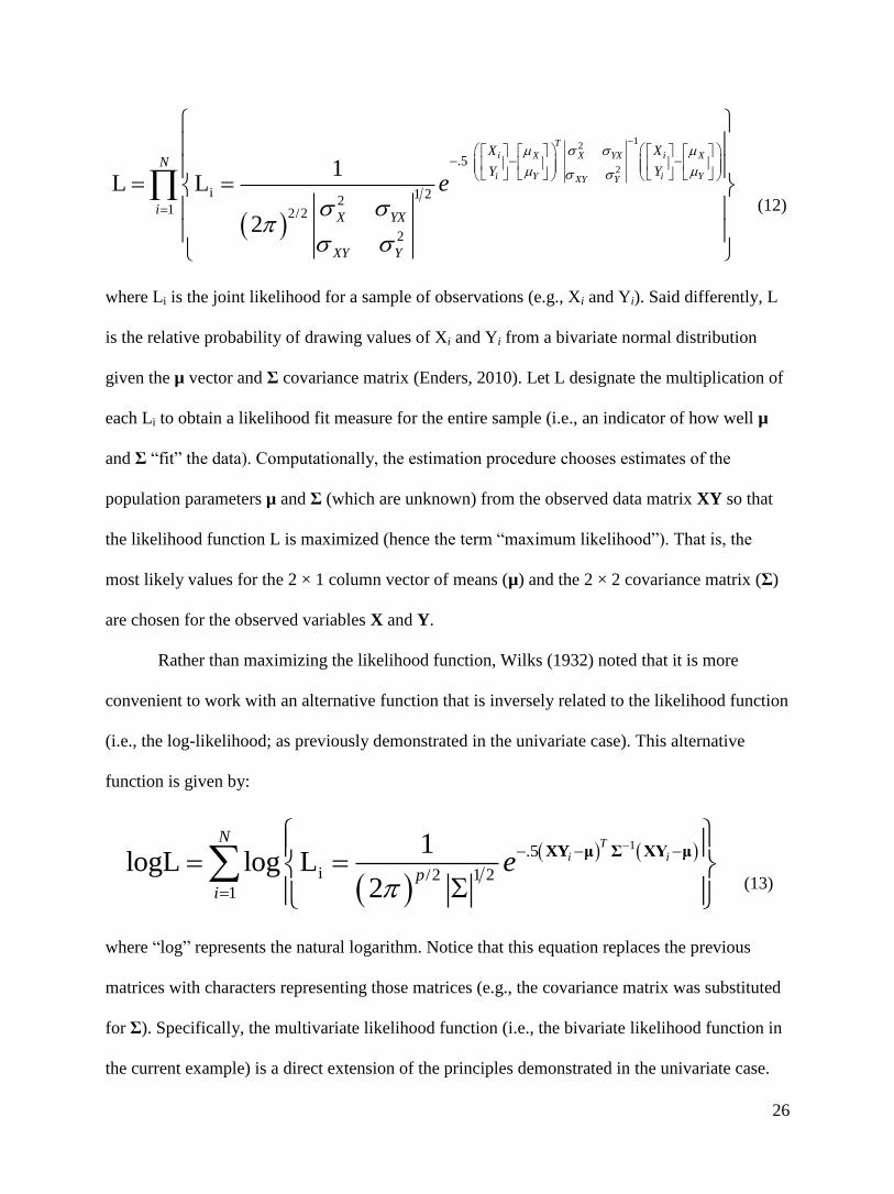
26

12

2.5

i 1 22

1 2/2

2

1L L

2

T

i iX X YX X

i iY YXY Y

X XN

Y Y

iX YX

XY Y

e

(12)

where Li is the joint likelihood for a sample of observations (e.g., Xi and Yi). Said differently, L

is the relative probability of drawing values of Xi and Yi from a bivariate normal distribution

given the µ vector and Σ covariance matrix (Enders, 2010). Let L designate the multiplication of

each Li to obtain a likelihood fit measure for the entire sample (i.e., an indicator of how well µ

and Σ “fit” the data). Computationally, the estimation procedure chooses estimates of the

population parameters µ and Σ (which are unknown) from the observed data matrix XY so that

the likelihood function L is maximized (hence the term “maximum likelihood”). That is, the

most likely values for the 2 × 1 column vector of means (µ) and the 2 × 2 covariance matrix (Σ)

are chosen for the observed variables X and Y.

Rather than maximizing the likelihood function, Wilks (1932) noted that it is more

convenient to work with an alternative function that is inversely related to the likelihood function

(i.e., the log-likelihood; as previously demonstrated in the univariate case). This alternative

function is given by:

1.5

i 1 2/21

1logL log L

2

T

i i

N

pi

e

XY μ Σ XY μ

(13)

where “log” represents the natural logarithm. Notice that this equation replaces the previous

matrices with characters representing those matrices (e.g., the covariance matrix was substituted

for Σ). Specifically, the multivariate likelihood function (i.e., the bivariate likelihood function in

the current example) is a direct extension of the principles demonstrated in the univariate case.

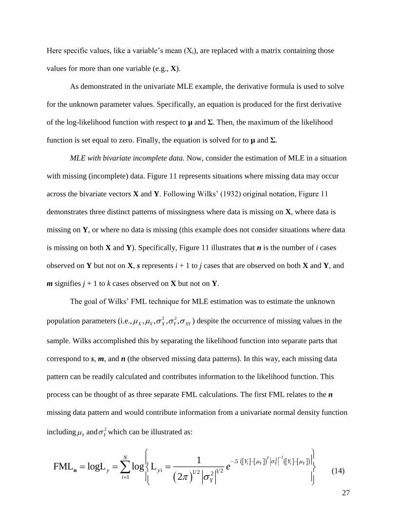
27

Here specific values, like a variable’s mean (Xi), are replaced with a matrix containing those

values for more than one variable (e.g., X).

As demonstrated in the univariate MLE example, the derivative formula is used to solve

for the unknown parameter values. Specifically, an equation is produced for the first derivative

of the log-likelihood function with respect to µ and Σ. Then, the maximum of the likelihood

function is set equal to zero. Finally, the equation is solved for to µ and Σ.

MLE with bivariate incomplete data. Now, consider the estimation of MLE in a situation

with missing (incomplete) data. Figure 11 represents situations where missing data may occur

across the bivariate vectors X and Y. Following Wilks’ (1932) original notation, Figure 11

demonstrates three distinct patterns of missingness where data is missing on X, where data is

missing on Y, or where no data is missing (this example does not consider situations where data

is missing on both X and Y). Specifically, Figure 11 illustrates that n is the number of i cases

observed on Y but not on X, s represents i + 1 to j cases that are observed on both X and Y, and

m signifies j + 1 to k cases observed on X but not on Y.

The goal of Wilks’ FML technique for MLE estimation was to estimate the unknown

population parameters (i.e.,2 2, , , ,X Y X Y XY ) despite the occurrence of missing values in the

sample. Wilks accomplished this by separating the likelihood function into separate parts that

correspond to s, m, and n (the observed missing data patterns). In this way, each missing data

pattern can be readily calculated and contributes information to the likelihood function. This

process can be thought of as three separate FML calculations. The first FML relates to the n

missing data pattern and would contribute information from a univariate normal density function

includingY and

2

Y which can be illustrated as:

1

2.5

i 1 21/2 21

1FML logL log L

2

T

i Y Y i Y

NY Y

y y

iY

e

n (14)

28

Likewise, the second FML relates to the m pattern and would contribute information from a

univariate normal density function including2 and X X ,

1

2.5

i 1 21/2 21

1FML logL log L

2

T

i X X i X

NX X

x x

iX

e

m (15)

Lastly, the third FML relates to the s missing data pattern and would contribute information from

a bivariate normal density function including2 2, , , ,X Y X Y XY , which is expressed as:

12

2.5

i 1 22

1 2/2

2

1FML logL log L

2

T

i iX X YX X

i iY YXY Y

X XN

Y Y

xy xy

iX YX

XY Y

e

s (16)

The likelihood function for the observed data is then maximized with respect to each of

the population parameters 2 2, , , ,X Y X Y XY . Specifically, Wilks (1932) used the ratios m/s

and n/s to weight the first derivatives of the parameter estimates prior to setting them equal to 0

and solving by approximation. Though, this idea was ahead of computational technology at the

time and would not become practical until the development of sophisticated iterative methods

and modern computers. Still, by incorporating FML information from each missing data pattern,

Wilks was able to demonstrate the mathematics behind a maximum likelihood missing data

estimation routine that effectively weights the FML solution 2 2ˆ ˆ ˆ ˆ ˆ, , , ,X Y X Y XY by using

information from each missing data pattern (i.e., FMLs, FMLm and FMLn). Conceptually, the

final FML solution is determined by combining all of these expressions where FML = FMLs +

FMLm + FMLn. That is, each of the FML parameter estimates are located using first derivatives

weighted by the observed information (see Wilks, p. 166).

29

Due to computational limitations, Wilks’ work on maximum likelihood estimation in the

presence of missing data remained largely undeveloped for nearly five decades until Anderson

(1957) and a few others worked to refine the technique (see Little & Rubin, 2002 for exceptions).

Anderson was among the first to apply maximum likelihood methods to an actual missing data

example (e.g., a simple situation with one missing value) by a non-iterative factoring technique

similar to that proposed by Wilks (see Dodge, 1985 for details). This approach allowed for an

ease in computational complexity but was limited to very specific missing data patterns. A short

time later, Hartley (1958) also added to work on maximum likelihood methods with an iterative

technique involving contingency tables. Later, Hartley and Hocking (1971) applied an iterative

maximum likelihood technique to multivariate normal data in the presence of missing data. Their

basic approach was similar to the original ideas described by Wilks (1932). For instance, Hartley

and Hocking separated the data into groups where each group represents a different missing data

pattern. Then, they maximized the likelihood function for each group (i.e., missing data pattern)

with respect to the population parameters. To illustrate how Hartley and Hocking (1971) selected

information for each of the missing data patterns, consider the data example shown in Appendix

C. As demonstrated in the previous discussion, Wilks (1932) can be seen as the origin for much

of the work on missing data in the context of maximum likelihood estimation. Still, this was not

his only contribution to the field. Mean substitution and pairwise deletion methods are discussed

next.

Simpler systems of estimates in the presence of missing data. Wilks (1932) was well

aware of the computational limitations of his time. As he noted, “in view of the difficulties

connected with the foregoing maximum likelihood estimates, we shall devote the remainder of

this paper to a consideration of the moments, distributions and efficiencies of simpler systems of

estimates,” (p. 178). The impending discussion covers Wilks’ simpler systems including pairwise

deletion and mean substitution. It is interesting to note that Wilks’ method of pairwise deletion is

30

still the default missing data handling procedure in many current statistical software programs,

despite its original purpose as essentially an alternative to cumbersome hand calculations.

Pairwise deletion. Conceptually, the maximum likelihood process described previously is

similar to the pairwise deletion method also outlined by Wilks (1932) though these approaches

are not mathematically associated (Enders, 2001). Rather than relying on a probability density

function to maximize the likelihood of the parameter estimates employing all of the observed

data, Wilks’ “less efficient but simpler” pairwise deletion method directly calculates each

covariance estimate from the available data. To illustrate consider the sample covariance ˆXY

and correlation XYr formula (Johnson & Wichern, 2002):

2 2

ˆ ˆ ˆ( )( )ˆ

1 ˆ ˆ

i X i Y XYXY XY

X Y

x yr

N

(17)

where ˆX is the mean of X, ˆ

Y is the mean of Y, 2ˆX is the variance of X,

2ˆY is the variance of

Y, and ˆXY is the covariance between X and Y. Now consider the pairwise deletion method

where 2 2ˆ ˆ ˆ ˆ ˆ, , , ,X Y X Y XY are each calculated based on all available data. This estimate

corresponds to the following (see Wilks, 1932):

2 2

ˆ ˆ ˆ( )( )ˆ

1 ˆ ˆ

i X i Y XYXY XY

X Y

x yr

N

s s ss s

s s s (18)

where N s is a set of cases with both ix and iy observed (e.g., s in Figure 11), and the means ˆXs

and ˆYs are typically calculated over that set of cases (Little and Rubin, 2002). However, it is

important to note uncertainty as ˆXs

could be calculated over all available i cases for x (e.g., s

and m in Figure 10). Likewise, the mean ˆYs

could also be calculated over all available i cases

for y (e.g., n and s in Figure 11). Therefore, pairwise deletion may use some cases in one part of

31

the sample covariance formula (e.g., the mean deviation) and another set of cases in another part

(e.g., the sample mean).

While this approach attempts to use all the available information, the generated

covariance matrix (which might then be used in a subsequent multivariate analysis) is based on

different subsets of cases. Frequently this situation results in negative eigenvalues (a non-

positive definite matrix; see Graham, 2009; Kline, 2011; Marsh, 1998; Wothke, 1993). As will

be discussed in detail later, an eigenvalue is essentially a variance term related to an optimally

weighted linear combination of the data and as such cannot be negative (see Jackson, 1991;

Johnson & Wichern, 2002). Said differently, the resulting covariance matrix might be internally

inconsistent because the range of possible values for a particular variance/covariance estimate

are not dependent on all of the other relationships in the matrix. For example, consider the

correlation between the variables X and Y ( XYr ) given the correlation between the variables X and

Z ( XZr ) and the correlation between the variables Y and Z ( YZr ) which can be written as (see

Kline, 2011; Kutner, Nachtsheim, Neter, and Li, 2005):

1 1XZ YZ XZ YZr r r r (19)

Now suppose XZr = .20 and YZr = .32 so that XYr must be greater than -.67 and less than .80 for the

matrix to remain invertible (i.e., positive definite). Additionally, Kline (2011) notes that, “…the

maximum absolute value of a covariance between any two variables is (must be) less than or

equal to the square root of the product of their variances,” (p. 50) which can be expressed as:

2 2ˆ ˆ ˆmax XY X Y (20)

where ˆXY is the covariance between X and Y,

2ˆX is the variance of X, and

2ˆY is the variance

of Y. When data are missing these invalid correlation matrices are possible when pairwise

deletion is used and can lead to subsequent intractable multivariate analyses since the data matrix

32

cannot be inverted via matrix algebra manipulations (Kline, 2011). Assuming a positive definite

covariance matrix, research thus far does not clarify how standard errors should be calculated

because the covariance matrix is not possible given any particular sample size (Allison, 2001;

Newman, 2003). As Enders (2010) pointed out, the pairwise deletion approach may lead to bias

and should be avoided.

Mean substitution. Another approach taken by Wilks (1932) was to replace the missing

values with the means from available cases. Applying the available case idea to the mean of X

ˆX and the mean of Y ˆ

Y yields:

1 1

1 1ˆ ˆ

N N

X i Y i

i i

x yN N

sm ns

sm ns

sm ns (21)

where N sm

is the set of observed x cases (i.e., s + m from Figure 11), and N ns is the set of

observed y cases (n + s from Figure 11). Once calculated ˆX and ˆ

Y are then used to replace

missing values for x and y respectively. Wilks’ noted that covariances can then be constructed

from the complete data such that the following formula is obtained for the covariance:

2 2

ˆ ˆ ˆ( )( )ˆ

1 ˆ ˆ

sm nssm ns i X i Y XY

XY XYsm ns

X Y

x yr

N

sm ns

(22)

Where ˆXsm

is the mean among all i observed x cases and ˆYns

denotes the mean among all i

observed y cases. Mean replacement may seem to make use of relevant information by replacing

missing values by the “most likely” value for that variable (its mean); however, mean

substitution has been shown to underestimate the variance and can attenuate relationships (see

Allison, 2003; Peugh & Enders, 2004). Enders (2010) notes that mean substitution is,

“…possibly the worst missing data handling method available,” (p. 43). That is, mean

substitution is likely to perform worse than deletion methods, despite the reason data are missing.

33

Missing information. Of the previously mentioned innovations provided by Wilks

(1932), each has found a place in current missing data handling approaches. For example,

likelihood-based approaches to address missing data are now common in most current statistical

software packages (e.g., Mplus, SAS, SPSS, etc.) and pairwise deletion is a popular default in

many programs (e.g., SPSS). In addition to these topics, another important advancement is worth

mention. Wilks (1932) introduced the idea of “estimation efficiency” in the presence of missing

data and described it mathematically as, “…the ratio of the reciprocal of the determinant of its

variances and covariances to that of the set of maximum likelihood estimates of the same

parameters,” (p. 171). To further this idea, consider that the determinant of a symmetric matrix

(such as a positive-definite covariance matrix) is equal to the product of its eigenvalues (Kolman,

1996; see subsequent PCA discussion for clarification) and reflects the amount of variance

information in the data.

While the idea of estimation efficiency employed by Wilks was to demonstrate the

potential effectiveness of maximum likelihood estimation over other possible methods, this paper

was perhaps the first to consider the concept of missing information, which was later developed

by Orchard and Woodbury (1972). Consider that Orchard and Woodbury, like Wilks, consider

the amount of variance information in a data set a measure of the certainty of parameter

estimates. To illustrate, consider that the information contained in a data set relates to the

steepness of the likelihood function (as described by Enders, 2010). That is, the steepness of the

likelihood function is related to the amount of information. Thus, the more information there is

to use, the more certain the parameter estimates will be. Figure 12 provides a depiction of this

concept.

Figure 12 includes two three-dimensional plots of a bivariate normal probability

distribution with variables X and Y where the density function ( , )f X Y represents the height of

the probability surface. Panel A of Figure 12 shows a high information and small standard error

34

condition. Here the likelihood function is steep. This situation would result in little ambiguity

regarding the most appropriate parameter estimates as the peeked likelihood surface indicates

greater precision (i.e., smaller standard error). In contrast, Panel B of Figure 12 demonstrates low

information and large standard errors reminiscent of a flat likelihood function. Parameter

estimates associated with this likelihood function are less clear than those in Panel A due to a

larger standard error.

Consider a more explicit illustration of this concept in relation to the univariate likelihood

function and associated first derivatives discussed previously. Figure 13 contains a series of plots

that demonstrate the relationship between the likelihood function and the first derivatives for two

different random samples. Panel A of Figure 13 relates to the data previously discussed for the

likelihood function of the mean from the column vector Y. Notice that this plot replicates Figure

8. Following the example provided by Enders (2010, p. 65-67), Panel B of Figure 13 represents a

likelihood function for the same mean but the data were generated to have a larger variance (i.e.,

2.5 times as large as Y).

As Enders (2010) notes, the flatter the slope of the regression line (Figure 13 bottom of

panel B), the less peaked the shape of the associated likelihood function (Figure 13 top panel of

B) relative to panel A. Figure 13 demonstrates that the curvature of the log-likelihood function

(i.e., the rate that the first derivative changes) directly reflects the standard error of a particular

maximum likelihood estimate of the mean (i.e., ˆY ). Said differently, as the likelihood function

becomes less peaked (i.e., flatter), many population values are possible which indicates more

difficulty deriving a precise maximum likelihood estimate (i.e., many first derivatives are close

to zero) and a larger standard error. Similarly, a likelihood function that is highly peaked offers

fewer possibilities for the population estimate. Thus, the associated standard error is smaller.

35

That is, standard errors are due to the relationship between the estimate precision (i.e., sampling

variance) and the likelihood function (see Enders, 2010).

To further this notion, note that the sampling variance of the mean can be written as:

1 12 2

2 2

logLˆvar

N

N

(23)

where ˆvar represents the sampling variance and 2 denotes the second derivative (see Enders,

2010). The second derivative estimate corresponding to Figure 13 is -3.33 and -1.33 for Panel A

and Panel B, respectfully. As noted these values represent the slopes of the log-likelihood

regression lines; see bottom of Panel A and B). Note that the slope plot in the bottom of Panel A

in Figure 13 is steeper than the associated plot in Panel B. As Enders demonstrated, multiplying

these derivative values by -1 (e.g., 3.33 and 1.33) yields an index of the information contained in

each likelihood plot. Further, the inverse of the information index is the sampling variance

estimates; which are .30 and .75 for Panel A and Panel B of Figure 13, respectively. Finally,

taking the square root of the sampling variance generates the standard errors. Therefore, ML

standard error-of-the-mean estimates are .55 for Panel A and .87 for Panel B of Figure 13.

Based on this discussion, it is appropriate to describe the steepness of the likelihood

function in relation to the amount of information in the sample data (as previously implied).

Orchard and Woodbury relate the concept of increased variance (i.e., larger ML standard errors)

to the loss of information caused by missing data (they referred to this as “hidden variance”). As

they note a small percent of missing data may introduce a large amount of hidden variance.

Missing information, Orchard and Woodbury (1972) argue, is a separate concept from

percent of missing data. More specifically, missing data have an influence on the efficiency of

parameter estimates to the degree that the missing information increases standard errors.

Importantly, this concept helped stimulate methodologists to develop estimation techniques (e.g.,

36

the EM algorithm) that include as much information as possible in the likelihood function as this

would provide a more precise point estimate and a smaller standard error than is possible with

less information (see Little & Rubin, 2002). Specific formulae related to formalizing the concept

of missing information will be discussed in relation to multiple imputation in forthcoming

discussion.

Summary of early developments. In the context of early developments in missing data

research, it was shown that the idea of missing data as a problem (i.e., a statistical hindrance)

seems to have its origins in the development and application of classical inferential statistics

which were designed for complete case (i.e., balanced) data. While the earliest missing data

techniques involved complete cases analysis (e.g., data deletion to obtain balance), simple

imputation methods were introduced as early as 1930. Discussion acknowledged that early

imputation approaches were comprehensively studied in the context of ANOVA, largely in

response to requests from applied researchers. Also, a maximum likelihood-based estimation

scheme appeared early on but suffered from computational limitations. Many of these early

developments in maximum likelihood estimation in the presence of missing data were developed

in response to computational limitations and many of the resulting solutions were situation

specific. That is, they were designed for a specific and often simplified type of missing data

pattern (which was not realistic in practice) or these methods were designed for a specific type of

data analysis and were not generalizable to other situations (see Little and Rubin, 2002). Much of

the general application of maximum likelihood estimation in the presence of missing data would

require computer implementation (e.g., iterative algorithms) which will be discussed later.

Importantly, many key ideas relating to missing data theory and application appeared

throughout the discussion of early methods. It seems that the idea of addressing missing data as a

potentially complex problem developed as researchers began to acknowledge that results vary as

a function of the information available and as a function of the analytic tools used to correct for

37

missing data. The next historical period will move missing data research forward by the

computational advancements provided by computers and also by questioning a commonly held

assumption that the process that caused missing data can be ignored.

The Second Historical Period: Ignorable Missing Data and Estimation

Donald Rubin (1976) appears to be the first to question the statistical literature’s adoption

of missing values as ignorable information. Rubin had already published a covariance procedure

to estimate missing data (see Rubin, 1972) and his 1976 article titled, “Inference and Missing

Data”, was a substantial achievement at the time as it effectively repositioned missing data

theory. This article provided the theoretical motivation and the statistical foundation for

understanding the relationship between “why the data are missing” and the ability to recover

missing data (i.e., the ability to make unbiased sampling distribution inferences). Rubin

emphasized that when researchers encounter missing data, incorrectly assuming that incomplete

data are missing at random (i.e., ignorable) may bias any inferences made from that sample. He

described that missing data cause deviations from probability sampling. Specifically, proper

randomization is a fundamental aspect of classical inferential procedures (i.e., Frequentist

approach to statistical inference) which can only be assumed when the missing values are

themselves an ignorable (e.g., random) form of probability sampling. For clarification, see the

brief example of this concept demonstrated in Appendix D.

The beginnings of a classification system. Rubin (1976) argues that typically when a

study contains missing data, the researcher is never sure which population is represented by the

observed sample. That is, the sample is typically selective due to the process that generated

missingness. Therefore, the observed sampling distribution could actually be a mixture of several

sampling distributions and any statistical inference based on a probability statement about a

particular distribution of the population would be inaccurate. As later described by Rubin and

Little (1987), “the key ingredient of the randomization approach, a known probability

38

distribution governing which values are unobserved, is lost when some of the data are missing,”

(p. 53). Rubin’s concerns about randomization and probability sampling in the context of

missing data introduced the beginnings of an essential classification system for missing data

(Enders, 2010; Little & Rubin, 2002) and greatly influenced the introduction of missing data as

an independent field of study within the social and behavioral sciences (see Molenberghs &

Kenward, 2007). The fundamental aspects of the classification system related to missing data

will be discussed and mathematically illustrated in a subsequent section based on a slightly

refined version outlined several years later in an influential book by Rubin and Little (1987).

Introduction of iterative algorithms. In the Much of the second half of Rubin’s (1976)

paper seems to formulate an argument in favor of a promising approach to maximum likelihood

estimation (MLE), which was published in a more developed form the following year by

Dempster, Laird, and Rubin (1977). Recall that MLE in the presence of missing data was already

an established idea (e.g., Anderson, 1957; Hartley, 1958; Hartley & Hocking, 1971; Wilks,

1932); however, it was not practical without sophisticated iterative computational routines. That

is, the application of MLE techniques in the presence of missing data usually require “…iterative

optimization algorithms to identify the most likely set of parameter values,” (Enders, 2010, p.

65). Said differently, not all likelihood functions can provide a closed-form solution (i.e., one

solvable equation) for the maximum likelihood value of a particular parameter.

Little and Rubin (2002) elaborate on the reason a closed-form MLE solution cannot be

obtained with missing data. They note, “patterns of incomplete data in practice often do not have

the particular forms that allow explicit ML estimates to be calculated by exploiting factorizations

of the likelihood,” (p. 164). They continue this discussion noting that even if the missing data

patterns were manageable (i.e., the observed data selection matrix can be specified); it is likely

that each partition of the likelihood function would not be orthogonal. Therefore, maximizing the

likelihood separately for each pattern (as demonstrated previously in the context of Wilks

39

technique for MLE estimation with missing data) would not actually maximize the overall

likelihood. Thus, iterative algorithms were needed to solve otherwise inestimable or at the least

extremely complex maximum likelihood calculations (Little & Rubin, 2002).

Defining an iterative algorithm. To further develop this idea, consider that an iterative

algorithm is a mathematical procedure that yields a sequence of improving approximate solutions

for an estimation problem where a final solution is based on a pre-specified termination criterion

that suggests solutions are no longer improving (see McLachlan & Krishnan, 2008). Consider the

following set of linear equations that must be solved via approximation because a closed-form

solution is not practical. Let these equations be:

12 2 1 14

6 12 8 2

2 4 14 8

x y z

x y z

x y z

(24)

where the values x, y, and z are unknown. Notice that substituting a particular value in for x, y, or

z would influence the other estimates and solutions. That is, each unknown cannot be easily

isolated to generate a closed-form solution (e.g., x = 6 + 2). Solving these linear equations by

trial and error is both inefficient and challenging. Therefore, consider an iterative approach that

begins with a simple rearrangement of equations such that (see Kline, 2010):

14 2 11.167 0.167 0.083

12 12 12

2 6 80.167 0.500 0.667

12 12 12

8 2 40.571 0.143 0.286

14 14 14

x y z y z

y x z x z

z x y x y

(25)

Now, insert a start value (i.e., an initial guess) for x, y and z. In the current example, suppose that

x0 = 0, y0 = 0, and z0 = 0 where the subscript “0” indicates the iteration number. Typically, zero is

an undesirable starting value but is chosen here for didactic purposes. Using these starting values

derives the following estimates for x, y and z:

40

0

0

0

1.167 0.167 0 0.083 0 1.167

0.167 0.500 0 0.667 0 0.167

0.571 0.143 0 0.286 0 0.571

x

y

z

(26)

The next sequence to improve the solution involves inserting these estimates for the values x, y,

and z back into the equation where:

1

1

1

1.167 0.167 0.167 0.083 0.571 1.147

0.167 0.500 1.167 0.667 0.571 0.798

0.571 0.143 1.167 0.286 0.167 0.357

x

y

z

(27)

Notice that after the first iteration the estimates for x, y, and z have been updated. This

iterative process of estimation and updating the values of x, y, and z is repeated until subsequent

changes in the estimates fall below some pre-specified criterion. Consider the first 10 iterations

in Table 2 to demonstrate this process. Here the estimated values for x, y and z change the most

in the first few iterations and do not change much after the eighth iteration. Given a termination

criterion of .001 (the cut point for no significant changes in newly estimated values), the current

iterative estimation routine would have converged (stopped) at the eighth iteration and exported

x8 = 0.986, y8 = 0.758, and z8 = 0.647 as a solution. The quality of an iterative solution depends

on the complexity of the estimation routine, starting values and the specific iterative algorithm

used (McLachlan & Krishnan, 2008). While the Newton-Raphson algorithm and other similar

iterative techniques generally served this purpose, a new technique was needed for missing data

situations that were otherwise too complicated to implement (see Watanabe & Yamaguchi, 2004

for elaboration).

Introduction of the Expectation-Maximization (EM) algorithm. Dempster, Laird, and

Rubin’s 1977 paper titled, Maximum Likelihood from Incomplete Data via the EM Algorithm,

provided such an iterative computation technique for MLE estimates. This paper described the

expectation-maximization (EM) algorithm essentially, as we know it today, as a two-step

41

iterative procedure that exploits regression based imputation and maximum likelihood estimation

in concert to address missing data. Dempster, et al., (1977) coined the term “EM” as an acronym

for the two-step iterative nature of the procedure and popularized the technique by clarifying the

relationship between iterations and the associated increase in parameter likelihood given the

observed data (Little & Rubin, 2002).

Dempster, Laird, and Rubin (1977) also illustrated the iterative process for maximizing

the likelihood of the covariance matrix and mean vector given the complete data and provided

numerous examples. The practicality of the EM algorithm lies in its ease of implementation

(Enders, 2001; 2010). As will be demonstrated, the expectation step of each iterative sequence

involves taking expectations over complete-data and the following maximization step simply

requires complete data maximum likelihood estimation, which is typically solved with a closed-

form mathematical function for the first derivative (see Enders, 2001).

While earlier methods for addressing missing data required that missing data occur in a

complete random fashion, a point criticized by Rubin (1976). The EM algorithm required a less

stringent assumption. Specifically, the causes and correlates of missing data are not necessarily

random but must be included in the estimation routine. This was a significant step forward in

coupling missing data theory with techniques for estimation in the presence of missing data.

Briefly, Dempster, Laird, and Rubin (1977) began with an initial estimate of the means

and covariance matrix, which provide sufficient statistics from the observed data. Missing values

are not included at this point (i.e., listwise deletion for missing values). The Expectation step (the

“E” in EM) uses these initial estimates to predict missing data in the observed data using a set of

regression equations. The result is a new data set with no missing values. The Maximization step

(the “M” in EM) then generates an updated set of sufficient statistics form this new data set. The

EM procedure is repeated until changes in the sufficient statistics from one M-step to the next

become trivial. The converged EM solution contains maximum likelihood estimates of the

42

sufficient statistics. Appendix E demonstrates this procedure using example data.

Importantly, rather than ignoring potential causes and correlates of missing data

(variables that may explain why data are missing), the EM algorithm may include this

information in the estimation of sufficient statistics. For example, if missingness on variable Y is

caused by another variable X, the EM based sufficient statistics can incorporate X, or any such

variable, by adding that variable to the likelihood function during the EM iterations. Said

differently, the maximum likelihood estimate of the covariance matrix and mean vector

generated by the EM algorithm can be informed by all available data and statistical modeling can

then proceed with the specific variables of interest.

The EM algorithm is considered an “indirect” approach (Enders, 2001) because the final

sufficient statistics must be used for other analyses such as factor analysis or used to impute a

final complete data set (i.e., stopping after the last “E” step). As an indirect approach to handle

missing data, the EM algorithm has some important limitations that did not adequately solve the

problem of estimation in the presence of missing data. For instance, while the EM algorithm is

fully capable of incorporating extra variables that are causes or correlates of missingness, it was

not designed to generate appropriate standard errors; which require a corrective bootstrapping

technique (see Enders & Peugh, 2004).

Specifically, when the EM sufficient statistics are used to impute a final complete data set

(i.e., final set of linear regression equations; “E” step) the variability observed during the EM

iteration process is not retained. Enders (2001; 2010) described this as filled-in values falling

directly on a regression line because the final imputation is based solely on the final set of

sufficient statistics (from the last “M” step).

Further, the literature is not clear about the appropriate sample size to reference with the

EM algorithm. For instance, Graham and Schafer (1999) relate the EM algorithm to pairwise

deletion noting, “…it is not clear what sample size should be ascribed to a covariance matrix

43

estimated by EM,” (p. 3). As will be subsequently demonstrated, these limitations coupled with

the desire for a “direct” approach, where missing data are addressed and parameter estimates are

estimated in a single step, would lead to a transition from the EM algorithm to the direct ML

approach (i.e., FIML).

Introduction of full-information maximum likelihood (FIML). An emphasis on maximum

likelihood estimation and advances in computer technology (especially in relation to matrix

algebra; see Jöreskog, 1967) came together a couple years after the introduction of the EM

algorithm. For instance, methodologists assimilated these ideas and considered iterative

parameter estimation techniques for the factor analysis model, which resulted in Carl

Finkbeiner’s, “Estimation for the Multiple Factor Model When Data Are Missing,” published

from his dissertation in 1979. This paper was essentially an extension of earlier work by Wilks

(1932; see acknowledgement in Finkbeiner, 1979) and introduced full-information maximum

likelihood (FIML; Enders, 2001) for use in factor analysis. As Enders (2001) noted, FIML is

conceptually the same approach taken by Hartley and Hocking (1971; whom extended the work

of Wilks as previously noted) where the data are separated the data into groups that represent

various missing data patterns. However, rather than generating a set of group-level likelihood

estimates FIML was designed to use individual (i.e., case specific) likelihood functions. As

Finkbeiner (1979) wrote, “the overall discrepancy function value is obtained by summing the n

casewise likelihood functions…” (p. 134) which can be expressed as:

1.5

i 1 2/21

1logL log L

2

T

i i i i i

i

N

pi i

e

Y μ Σ Y μ

(28)

where ip represents the number of complete data points for individual (i.e., case) i, and iY denotes

the data for the thi individual (i.e., case). In addition, the mean vector i and the covariance

44

matrix i represent parameters unique to each case. Said differently, i and i may contain j

variables for a particular case but may contain k variables for another case where j k (see

Allison, 2002; Enders, 2010; Little & Rubin, 2002; Peugh & Enders, 2004). Note the similarity

of this equation to the complete data MLE formula. As Enders (2010) notes, the only difference

is that this formula does not contain the extra subscript i for the population parameters.

FIML is considered a model-based approach because missing data are handled within a

single, iterative step where missing values are not imputed (Graham, Cumsille, & Elek-Fisk,

2002). Rather, model parameters and standard errors are directly estimated from the observed

data of each individual case. In this way, the Finkbeiner paper marks a contrast from Dempster,

Laird, and Rubin’s (1977) EM algorithm approach to correcting for missing data. Specifically,

the EM algorithm generates MLE of the population parameters ( , ) which are then used as

sufficient statistics for further analyses. By comparison, FIML directly estimates a statistic and

its associated standard error from the data. Consequently, FIML is considered a direct approach

and is often referred to in the literature as direct-maximum likelihood (direct ML; e.g., Enders,

2001; 2010).

To compare this approach to other techniques used previously, consider that FIML is

similar to pairwise deletion in that both procedures use all the available data on a case wise basis

(Enders, 2001). However, FIML does not simply perform a direct calculation of each covariance

estimate from the available data. Rather, the FIML procedure relies on a probability density

function to iteratively maximize the likelihood of the estimates employing, “…all of the

information of the observed data, including mean and variance for the missing portions of a

variable, given the observed portion(s) of other variables,” (Wothke, 2000, p. 3). Consequently,

FIML, unlike pairwise deletion, uses the appropriate sample size for standard error estimates

(Allison, 2003; Enders, 2001) and is less likely to produce a non-positive definite matrix

45

(Wothke, 1993). FIML is considered “state of the art” in correcting for missing data (Enders &

Peugh, 2004; Schafer & Graham, 2002) because it can adequately recover key information, and

is based on a sound theory, unlike many of the more traditional methods for addressing missing

data (see Baraldi & Enders, 2010; Collins, Schafer, & Kam, 2001). For these reasons,

methodologists typically recommend FIML over traditional methods (see Graham, 2009 for

exceptions).

Researchers have investigated many aspects of FIML estimation though simulation

studies (e.g., Arbuckle, 1996; Enders & Bandalos, 2001; Peugh & Enders; Wothke, 2000) and

describe the technique as unbiased and efficient (i.e., produces a small standard error relative to

preceding missing data methods) given that certain assumptions are met. Specifically, FIML

requires a relatively large sample size (see Schafer & Graham, 2002 for details), a multivariate

normal distribution (Enders, 2010), and the cause of missingness must be included in the

estimation procedure.

Of these assumptions ensuring that the causes and correlates of missing data are included

in the FIML likelihood function is typically the most challenging (Enders, 2010; Enders &

Bandalos, 2001; Little & Rubin, 2002; Schafer & Graham, 2002; Wothke, 2000). FIML

estimation is thought to be relatively robust to violations of normality and small sample sizes.

For instance, methodologists have noted that FIML is likely robust to mild and even moderate

violations of multivariate normality (e.g., Enders, 2010) and severe non-normality can be

addressed via one of many modified FIML estimation routines that are robust to non-normality

(e.g., Muthén & Muthén, 2011).

However, as a direct approach for addressing missing data, the FIML procedure only

incorporates variables that are directly modeled. For example, FIML only integrates information

from variables that are referenced in the linear model investigated (e.g., multiple regression,

factor analysis, etc.). To illustrate this concept, see Appendix F, which demonstrates how

46

Finkbeiner (1979) applied FIML to the factor analysis model.

The inability of the FIML procedure to include all possible causes or correlates of

missingness was initially a significant limitation (see Enders, 2001). However, this drawback

was addressed in the literature when Graham (2003) provided effective, though somewhat

complex procedures to incorporate extra “auxiliary” variables into the FIML estimation routine

without modifying the basic statistical model under investigation. This concept is discussed in

more detail throughout the forthcoming sections.

Summary of ignorable missing data and estimation. As discussed, the traditional

methods for handling missing data, though easy to implement by hand calculation, often place

the researcher in a position to be the most wrong that he/she can possibly be because most

missing data are not ignorable (Rubin, 1976). To avoid methods that attempt to edit the observed,

incomplete dataset by filling in missing data or deleting data (e.g., single regression imputation,

listwise deletion, pairwise deletion, and mean substitution), researchers turned toward iterative

estimation techniques that are based on methodological theory rather than computational

convenience.

Due to Rubin’s (1976) introduction to modern thinking about missing data and advances

in computer technology, methodologists assimilated the EM algorithm and a short time later

FIML. The difference in substitution procedures like single regression imputation and

approaches like EM algorithm or FIML relates to the sophistication involved in generating

plausible values. These methods do not assume that the data are missing completely at random

and are able to incorporate the cause of missingness in the estimation procedure. That is, despite

the noted limitations EM and FIML can more adequately recover key information, and are based

on statistical theory, unlike many long-standing traditional approaches like deletion and single

imputation (Graham, 2009; Schafer & Graham, 2002).

The following historical period will highlight further developments in missing data

47

estimation, including the introduction of a new technique called multiple imputation.

Additionally, the rising field of missing data research asserts influence in thinking about missing

data throughout the social and behavioral sciences by producing a series of widely influential

books and articles. The implementation of appropriate missing data techniques like FIML

become more common with the introduction of less technical computing software programs

primarily intended for applied researchers.

The Third Historical Period – A Revolution in Missing Data

As Graham (2009) noted, “problems brought about by missing data began to be

addressed in important ways starting in 1987, although a few highly influential articles appear

before then,” (p. 550). In particular, two persuasive books appeared on the topic of missing data

including Little and Rubin (1987), and Rubin (1987); additionally, two prominent papers also

emerged with Allison (1987), and Tanner & Wong (1987) among others that same year. These

publications provided the social and behavioral sciences with formal discussions and

demonstrations that linked missing data research with work on statistical modeling and the

computational advancements provided by personal computers at the time (see Enders, 2010;

Graham, 2009; Little, 2011). For instance, Allison’s (1987) paper titled, “Estimation of linear

models with incomplete data,” implemented maximum likelihood with missing data (as derived

by Hartly & Hocking, 1971 and shown by Finkbeiner, 1979) in the LISREL software package

for estimating structural equation models (SEM). In addition to a mathematical demonstration of

this technique with matrix algebra, Allison also included appendices with LISREL code and

example data. These appendices reflect the aspirations of the larger missing data field to bridge

the gap between theoretical suggestions on handling missing data and practical applications.

The following discussion touches on some relevant aspects of these works and

demonstrates a discernible turning point in the understanding and acceptance of missing data

theory and the implementation of “modern” missing data handling techniques.

48

Theoretical overview of missing data mechanisms. When researchers encounter

missing data, the recoverability of that information is related to the missing data mechanisms or

“why the data are missing” (Enders, 2010). If the social scientist, or any other scientist, can

determine why data are missing, they can recover the lost information (Little & Rubin, 2002).

That is, the researcher can determine what missing scores would have been had the participant

remained in the sample. However, when the cause of missingness is not explained (i.e., variables

responsible for missing data are not included in the missing data handling procedure) the

recoverability of lost information is severely limited, as will be explained in the forthcoming

discussion. The theoretical ability of a researcher to recover lost information is important for

choosing a missing data handling procedure and subsequently deriving appropriate statistical

inferences (Enders, 2010).

Rubin’s (1976) earlier discussion of the recoverability of missing data in relation to the

cause of missingness was formalized and termed “missing data mechanisms” in Roderick Little

and Donald Rubin’s 1987 book, “Statistical Analysis with Missing Data” (the second edition was

published in 2002). The missing data mechanisms outlined by Little and Rubin (1987; 2002),

include concepts that are prevalent today as a theoretical foundation for understanding and

appropriately handling missing data (see Enders, 2010).

Defining missing data mechanisms. Little and Rubin (1987; 2002) refined Rubin’s

(1976) probability theory discussion and formalized three basic mechanisms that cause

missingness to arise in a research study. These missing data mechanisms include data that are

missing completely at random (MCAR), data that are missing at random (MAR) and data that are

missing not at random (MNAR). This section will introduce each of these missing data causes

and demonstrate data examples in turn. As will be shown, the distinctions between these

mechanisms involve the relationship between the probability of missingness and the data.

49

Consider that when data are missing, the original rectangular data matrix is unbalanced

since the original i measurements on p variables are not completely observed. Figure 14 shows

an exemplar data matrix with missing values and provides notation that will be referenced

throughout the forthcoming discussion. Specifically, let Y in Figure 14 illustrate an i x p data

matrix with missing values and allow matrix R to be an i x p missingness indicator matrix where

observed values in matrix Y are represented by 1’s and missing values in matrix Y are 0’s (or

vice versa).

The matrix R indicates the probability data are missing, which is denoted by P(R),

because it refers to a matrix of indicator variables with a probability distribution (Little & Rubin,

1987, Rubin, 1976). To develop the concept of the probability distribution of the matrix R, recall

Rubin’s (1976) argument that the observed probability distribution of a sample with missing data

could actually be a mixture of several probability distributions. Explicitly stated, when missing

data are present the researcher is unsure which population is represented by the observed sample.

To address this issue, Rubin (1976) suggests defining missing data as a variable (i.e., R) because

variables have a probability distribution that can be subsequently described by an equation. That

is, P(R) can be expressed as a function of the data through the conditional distribution of R given

Y. As will be revealed in the following discussion, missing data mechanisms are fundamentally

assumptions about the independence of these probability distributions. As Enders (2010) noted,

“the formal definitions of missing data mechanisms involve different probability distributions for

the missing data indicator, R,” (p. 10). To solidify the idea of probability distributions in this

context, consider the graphical example presented in Appendix G.

An important point made by Rubin (1976) is that variables that a researcher does not

measure may significantly influence those variables that are measured. Therefore, any discussion

of missing data causes must consider all possible factors that may influence the probability

distribution of R. Prior to expressing each missing data mechanism; consider the theoretical

50

overview of the missing data mechanisms outlined in Figure 15. This figure presents a

framework for missing data mechanisms that highlights the relationship among Yp and R in

relation to measured (Yobs) and unmeasured data (Ymis).

Specifically, Figure 15 is composed of four portions including: (1) MCAR, (2) MNAR,

(3) MAR and (4) MAR / MNAR. These sections form a grid that identify the missing data

mechanism associated with observed and unobserved that are either dependent or independent of

the probability of missingness. For instance, the top left panel of Figure 15 corresponds to the

MCAR mechanism and represents a situation with independent probability distributions (i.e., a

condition of “no association”). All other panels denote some level of relationship between R and

the data. As will be discussed, in order for a researcher to assume that a particular population is

represented by an observed sample with missing data; the data must be shown to be independent

or predictive of R. Otherwise, the sample would include the possibility of severe bias due to

selectivity (e.g., selective attrition).

Missing completely at random (MCAR). Missing data are missing completely at random

(MCAR) when missingness is due to a truly random process (Little & Rubin, 1987, 2002). That

is, the probability that a value is missing (R) is unrelated to the observed data (Yobs) and also

unrelated to unmeasured data (Ymis). Mathematically, MCAR can be expressed as:

( | , , ) ( | )obs misP Y Y P R R (29)

where R denotes the probability of missingness, Yobs and Ymis reference the data, and ϕ is a

parameter that describes the relationship between R and the data (Enders, 2010; Little & Rubin,

2002). This equation indicates that the probability of missingness, R, given Yobs and Ymis (the left

side of the equal sign) is simply equal to the probability of missingness (the right side of the

equal sign). Note that ϕ merely describes the mathematical connection between R and the data

regardless of the relationships (i.e., random or predictive).

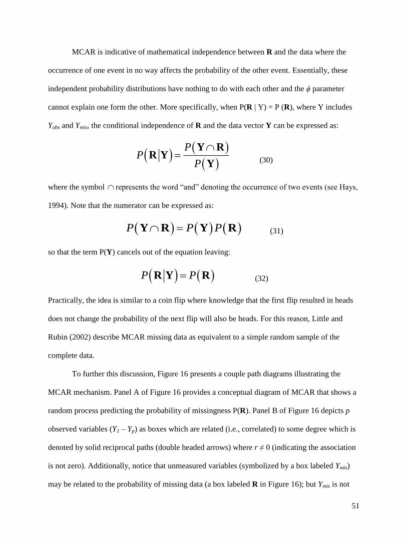
51

MCAR is indicative of mathematical independence between R and the data where the

occurrence of one event in no way affects the probability of the other event. Essentially, these

independent probability distributions have nothing to do with each other and the ϕ parameter

cannot explain one form the other. More specifically, when P(R | Y) = P (R), where Y includes

Yobs and Ymis, the conditional independence of R and the data vector Y can be expressed as:

PP

P

Y RR Y

Y (30)

where the symbol represents the word “and” denoting the occurrence of two events (see Hays,

1994). Note that the numerator can be expressed as:

P P P Y R Y R (31)

so that the term P(Y) cancels out of the equation leaving:

P PR Y R (32)

Practically, the idea is similar to a coin flip where knowledge that the first flip resulted in heads

does not change the probability of the next flip will also be heads. For this reason, Little and

Rubin (2002) describe MCAR missing data as equivalent to a simple random sample of the

complete data.

To further this discussion, Figure 16 presents a couple path diagrams illustrating the

MCAR mechanism. Panel A of Figure 16 provides a conceptual diagram of MCAR that shows a

random process predicting the probability of missingness P(R). Panel B of Figure 16 depicts p

observed variables (Y1 – Yp) as boxes which are related (i.e., correlated) to some degree which is

denoted by solid reciprocal paths (double headed arrows) where r ≠ 0 (indicating the association

is not zero). Additionally, notice that unmeasured variables (symbolized by a box labeled Ymis)

may be related to the probability of missing data (a box labeled R in Figure 16); but Ymis is not

52

related to Y1 – Yp. Therefore, any influence from Ymis to R does not impact Yobs (i.e., Y1 – Yp).

Therefore, these components are independent (shown by dotted reciprocal paths) where r = 0

(suggesting no association). Essentially, P(R) described by the parameter ϕ is unrelated to

measured or unmeasured systematic processes (i.e., missingness is completely random).

For example, suppose that data on language outcomes (i.e., Y1 – Yp) among children are

missing for a subset of participants. More specifically, let Y2 represent a particular variable with

missing data while the other outcomes are completely observed. As previously discussed, R

describes the propensity for missing data. That is, R represents the reason that children did not

provide responses to Y2.

Now, suppose that there are unmeasured reasons (Ymis) for this missing data. For

example, assume that a few children did not understand the Y2 item, that the assessor

(investigator) accidently skipped Y2 for some participants, or that some children got bored and

stopped participating in the language assessment, alternatively perhaps children were distracted

by some random occurrence. These situations may cause missing data R (denoted by r ≠ 0 in

Figure 16 between R and Ymis); however, notice that in Figure 16 there is no systematic

relationship between R and the language outcomes (Y1 – Yp). In words, there are reasons for

missing data but missingness on a particular variable (i.e., Y2) is not systematically related to

measured or unmeasured variables. The cause of missingness is random.

All missing data handling procedures (e.g., likelihood-based techniques, data

augmentation techniques, deletion techniques, etc.) assume at least the MCAR level of missing

data and almost any missing data technique will lead to unbiased results given this type of

missing data (Enders, 2010; Graham, 2009; Little & Rubin, 2002). That is, when missing data

are MCAR, the researcher can completely recover the lost information from the remaining data.

That is, there are no systematic causes of missingness so the probability distribution of R is

simply a random sample of the data. However, some missing data handling procedures are still

53

preferable. For instance FIML is preferred over deletion techniques due to an increase in

statistical power (Enders, 2010).

To demonstrate a data example of MCAR, consider a research scenario where it is of

interest to estimate the relationship between two random normal variables, Y1 and Y2. These

artificial data contain N = 30 cases and are included in Table 3, where the correlation is 12 .67r

when the data are complete. This table will be referenced throughout the discussion of all

missing data mechanisms for instructive purposes. Now suppose that all values of the variable Y1

are observed and only some of the values of Y2 are observed. Figure 17 summarizes this

univariate missing data pattern. Specifically, there are m cases of Y2 and p cases of Y1.

Numerous research situations that lead to this pattern of missing data (see Little and

Rubin, 1987; Enders, 2010). For instance, let Y2 represent a questionnaire item with missing data

and let Y1 represent a demographic variable, like age, with no missing values. The variable Y1

could also represent a fixed variable controlled by the experimenter or any other variable with

complete data. In order to illustrate the benign nature of MCAR missingness, let Y2 contain 50%

MCAR missingness (i.e., missingness is generated completely at random; see Table 3). Note that

in Table 3 the mean (M = -.02) and standard deviation (SD = 1.0) of Y2 under MCAR are close to

the complete data estimates (.04 and .89, respectively) despite the sample missing half of the

observations (i.e., N = 15). Additionally, as noted in Table 3, the correlation between Y1 and Y2 is

r = .67 in the complete data situation and r = .69 in the 50% MCAR situation.

Missing at random (MAR). Rubin (1976) noted that missing data that is a completely

random process is unrealistic except under planned missing data designs (see Graham, Taylor, &

Cumsille, 2001 for details). Rather missing data are typically related to selective (i.e., systematic)

processes. This idea is essential for understanding the second mechanism, missing at random

(MAR). MAR does not actually propose that the data are missing at random; rather, it means that

the data are missing for a reason and the researcher happens to know the reason (Enders, 2010;

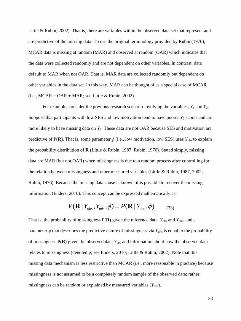
54

Little & Rubin, 2002). That is, there are variables within the observed data set that represent and

are predictive of the missing data. To use the original terminology provided by Rubin (1976),

MCAR data is missing at random (MAR) and observed at random (OAR) which indicates that

the data were collected randomly and are not dependent on other variables. In contrast, data

default to MAR when not OAR. That is, MAR data are collected randomly but dependent on

other variables in the data set. In this way, MAR can be thought of as a special case of MCAR

(i.e., MCAR = OAR + MAR; see Little & Rubin, 2002).

For example, consider the previous research scenario involving the variables, Y1 and Y2.

Suppose that participants with low SES and low motivation tend to have poorer Y2 scores and are

more likely to have missing data on Y2. These data are not OAR because SES and motivation are

predictive of P(R). That is, some parameter ϕ (i.e., low motivation, low SES) uses Yobs to explain

the probability distribution of R (Little & Rubin, 1987; Rubin, 1976). Stated simply, missing

data are MAR (but not OAR) when missingness is due to a random process after controlling for

the relation between missingness and other measured variables (Little & Rubin, 1987, 2002;

Rubin, 1976). Because the missing data cause is known, it is possible to recover the missing

information (Enders, 2010). This concept can be expressed mathematically as:

obs( | , , ) ( | , )obs misP Y Y P Y R R (33)

That is, the probability of missingness P(R) given the reference data, Yobs and Ymis, and a

parameter ϕ that describes the predictive nature of missingness via Yobs is equal to the probability

of missingness P(R) given the observed data Yobs and information about how the observed data

relates to missingness (denoted ϕ; see Enders, 2010; Little & Rubin, 2002). Note that this

missing data mechanism is less restrictive than MCAR (i.e., more reasonable in practice) because

missingness is not assumed to be a completely random sample of the observed data; rather,

missingness can be random or explained by measured variables (Yobs).

55

Figure 18 presents a path diagram of the MAR mechanism. Panel A of Figure 18 offers a

conceptual diagram MAR that shows observed variables (Yobs) predicting the missing data (R).

Panel B of Figure 18 illustrates MAR in relation to p variables where Y2 contains missing data.

As demonstrated, R is can be associated with all variables except Y2. Note that R may influence

Y2 through other correlated variables. That is, missingness on Y2 may be caused by values on any

other p variable in the observed data matrix Y (e.g., the lower distribution of Y1 may cause

missingness on Y2, etc.). Since any such relationship among these p variables and Y2 are observed

the missing information can be recovered via ϕ.

To provide a demonstration of the MAR mechanism, suppose again that data on language

outcomes (i.e., Y1 – Yp) among children are missing for a subset of participants. Once more, let Y2

represent a variable with missing data while the other variables are observed. In Figure 18, R

represents the reason that children did not respond to Y2. This time suppose that there is a

relationship between missingness on Y2 and another measure called English Language Learner

(ELL; where Yp = ELL), such that participants that do not speak English well are less likely to

respond to Y2. In this case, there is a systematic relationship between R and the missing data.

That is, this relationship can be described by the parameter ϕ because ELL status is among the

outcome measures. That is, the reason why data are missing is because of ELL status; and ELL

status can be used to predict (i.e., explain) missing data. Modern missing data handling

procedures come in handy when the data are MAR because these procedures can successfully

recover missing information by utilizing the parameter ϕ. In contrast, traditional missing data

techniques are biased when the data are MAR because these techniques are unable to relate P(R)

to Yobs (Enders, 2010).

To demonstrate MAR with data, consider the 50% MAR data example in Table 3. Under

the MAR mechanism, missingness on the variable Y2 was generated from the lower distribution

of the variable Y1. More specifically, values of Y2 were deleted if the observed values of Y1 were

56

less than or equal to .20 (see Table 3). Among other things, this procedure mimics a scenario in

which missing values on a variable (i.e., Y2) result from low scores on another variable in the

data set. Because Y1 and Y2 were highly and positively correlated in the complete data example (

12 .67r ) deleting based on the lower distribution of Y1 effectively deletes from the lower

distribution of Y2. As demonstrated in Table 3, the result is that the mean of Y2 (M = .54) is too

large and the standard deviation (SD = .77) is too small. Additionally, note that the correlation

between Y1 and Y2 is 12 .19r in the 50% MAR situation (see Table 3). While these raw

differences are dramatic, modern missing data handling techniques can recover the lost

information (given adequate sample size). That is, ϕ can explain that missingness on the variable

Y2 was generated from the lower distribution of the variable Y1 (i.e., that low scores on one

variable relate to low scores on the other, etc.).

Missing not at random (MNAR). Missing data are missing not at random (MNAR) when

missingness is not completely random and not explained by measured variables (Little & Rubin,

1987, 2002). That is, there are unmeasured variables (Ymis) that explain the occurrence of

missing data. Essentially, the data are missing for a reason and the research does not have a

measure of that reason (i.e., no variables in the data set represent or are predictive of the missing

data). According to Enders (2010) missing data default to the MNAR mechanism when the data

are not randomly collected (i.e., selective attrition, etc.) and are not observed at random (i.e., no

observed variables explain the probability of missingness). Stated simply, the OAR concept does

not apply (see Little & Rubin, 2002). This mechanism can be written as:

( | , , ) ( | , , )obs mis obs misP Y Y P Y Y R R (34)

That is, the probability of missingness R is related to unmeasured variables (Ymis) and perhaps

measured variables (Yobs) as well (see Enders, 2010; Little & Rubin, 2002). Importantly, the

parameter ϕ is unable to describe a relationship between R and unmeasured variables. Said

57

differently, missingness on Y2 depends on Y2 itself (e.g., if participants who have lower Y2 scores

are never tested because they avoid being measured). These data are not collected randomly

because another process beyond Y1 - Yp generated missing data. If there is a reason for missing

data and the researchers do not have a measure of it missingness cannot be explained and the

recoverability of lost information is severely limited (Enders, 2010; Little, 2009).

Consider another example relating to the previously mentioned research scenario

involving the variables, Y1 and Y2. As before, let participants with low SES and low motivation

have poorer Y2 scores, and be more likely to have missing data on Y2. This time, however,

suppose that SES and motivation are not included in the data set. In this scenario, the observed

data probability distribution can be thought of as a combination of multiple probability

distributions where the sample data is not representative of any particular population and

therefore any statistical inferences based on a particular population are biased (Schafer, 1997).

That is, because the intended sample is selective and likely unrepresentative, the MNAR

mechanism is considered non-ignorable (Enders, 2010; Little & Rubin, 2002; Schafer, 1997).

Figure 19 illustrates a path diagram of the MNAR mechanism. Panel A of Figure 19

provides a theoretical explanation of MNAR. Here unmeasured variables (denoted Ymis) predict

(i.e,. cause) missingness. Also note that observed variables (Yobs) may also predict missingness

but strictly speaking, Yobs and Ymis are not related. That is, the observed variables are unable to

explain the missing data process. Panel B of Figure 19 shows the MNAR mechanism in relation

to p variables where Y2 contains missing data. Notice that R is associated with Y2. This situation

implies that information from Ymis relates to the observed missingness because the lost

information on the variable Y2 depends on the probability distribution of Y2 itself (Enders, 2010).

Continuing with the ongoing example regarding language outcomes, suppose that

participants whom would have scored in the lower distribution of the variable Y2 failed to

respond to that variable. This relationship is illustrated as a solid reciprocal relationship where r

58

≠ 0 between R and Y2 in Figure 19. In this case, missing data on Y2 is directly related to the

underlying values of Y2. In this situation, there is a systematic relationship between R and the

missing data but the investigators do not have a measure of it. Therefore, the parameter ϕ is

unable to describe the relationship that generated the missing data (the ϕ parameter is

uninformative). So, the sampling distribution of Y2 is biased because it does not contain the

lower distribution of Y2. Any inferences made based on Y2 are incorrect representations of that

sample.

To demonstrate the MNAR mechanism with example data, consider the 50% MNAR data

example in Table 3. Under the MNAR mechanism, missingness on the variable Y2 was generated

from the lower distribution of the variable Y2. More specifically, values of Y2 were deleted if the

observed values of Y2 were less than or equal to .07 (see Table 3). As demonstrated in Table 3,

the result is that the mean of Y2 (M = .71) is the largest and the standard deviation (SD = .51) is

the smallest. Additionally, note that the correlation between Y1 and Y2 is 12 .67r in the complete

data situation and 12 .40r in the 50% MNAR situation (see Table 3). Unfortunately, missing

data handling techniques are generally unable to recover information lost through the MNAR

mechanism. That is, ϕ cannot explain that missingness on the variable Y2 was generated from the

lower distribution of Y2 itself.

Using the previously described mechanisms, MCAR and MAR describe missing

information that is recoverable which means that P(R) can be ignored when making statistical

inferences based on the sample (Schafer, 1997). In contrast, methodologists note that the MNAR

mechanism designates a severe limitation to the recoverability of lost information, which

suggests that P(R) cannot be ignored because the resulting inferences are biased (see Enders,

2010). The fact that missing data can be grouped into ignorable and non-ignorable groups leads

to the quandary of what to do when the data are non-ignorable (i.e., MNAR).

59

Methodologists refer to this as a widely misunderstood concept because missingness is

typically a mixture of each mechanism (Enders, 2010; Graham, 2009; 2012). Pure mechanisms

are unlikely in practice. The following section develops the concept of MAR and MNAR that are

not distinct entities. Rather, these mechanisms are discussed in a more practical fashion in line

with Graham’s (2012) suggestions where MAR and MNAR form a continuum that cannot be

easily teased apart.

The MNAR to MAR continuum. It follows from the above discussion that most, if not all,

missing data situations involve a particular combination of missing data mechanisms (Graham,

2012; Yuan & Bentler, 2000). Figure 20 (adapted from Little, 2009) illustrates a theoretical

overview of these missing data mechanisms, which will guide the forthcoming discussion. Note

that in Figure 20, each mechanism contributes to the total percentage of missing data (illustrated

by predictive arrows). Specifically, the total percent of missing data within a particular set of

variables (termed, “Missing Data” in Figure 20) can be thought of as regressed on each of the

three mechanisms where the weight of each regression coefficient varies depending on the

particular variables selected from the larger data set. It is unclear how much of the total missing

data is related to each mechanism, as this would vary in a given study.

In Figure 20, notice that MCAR and MAR are described as ignorable mechanism, while

MNAR is denoted as non-ignorable; as previously discussed. Additionally, note the reciprocal

relationships (i.e., double-headed arrows) in Figure 20. These paths illustrate no theoretical

relationship between MCAR and the other mechanisms but a relationship of some magnitude

between MAR and MNAR. This image demonstrates the point that MAR and MNAR are not

distinct entities but are related.

To understand the relationship between MAR and MNAR (and lack of a relationship with

MCAR), recall that each mechanism rests on an unlikely assumption. For instance, MCAR

requires that missingness is completely random, which is only the case in planned missing data

60

designs that have no other missing data (Enders, 2010; Rubin, 1976). MAR requires that the

researcher measure and include in the missing data estimation routine all reasons that cause

missingness. Lastly, the MNAR situation involves unknown variables.

The only testable mechanism is MCAR (the randomness of R can be assessed; see Little,

1998; Enders, 2010). Unfortunately, it is not possible to demonstrate that a particular variable (or

set of variables) is the sole cause of missingness. Testing this assumption (that all variables

responsible for missing data are recorded in the researcher’s dataset) would require the missing

values to be isolated from the influence of all other possible causes (Enders, 2010). Given that

researchers are typically unaware of the precise causes of missing data, methodologists describe

this as “an ultimately untestable assumption,” (see Enders, 2010).

Thinking more about the relationship between MAR and MNAR consider that they are

more reasonably imagined as a continuum rather than as distinct entities because in reality

missingness related to these mechanisms cannot be isolated. Figure 21 explicitly shows the

relationship between MAR and MNAR to illustrate that virtually all missing data situations are

partially MAR and partially MNAR (recall MCAR is ignorable and is thus not relevant for the

current discussion).

Imagine that a given set of variables selected from a larger data set for analysis exists

somewhere along the continuum in Figure 21. That is, the more that P(R) is explained by the

observed data the closer the researcher moves on the continuum from MNAR toward MAR and

the less likely inferences are to be biased. This situation lead Enders (2010) to note, “collecting

data on the causes of missingness may effectively convert an MNAR situation to MAR,” (p. 15).

Also consider that some variables in the larger data set are more informative than others and the

researcher’s ability to more away from biased inferences is impacted by the ability to explain the

cause of missing data. As the research includes more information in the missing data handling

routine he/she moves closer to unbiased inferences.

61

Consider that methodologists recommend modern missing data handling techniques (e.g.,

FIML) with the idea that the MAR assumption is satisfied. That is, researchers have in the larger

data set and use in the modern missing data handling technique all relevant information such that

the researcher positions him/herself completely to the MAR side of the continuum. In order to

improve the likelihood of meeting this assumption (which is almost never actually met in

practice), a strategy has emerged where researchers intentionally include extra variables

(auxiliary variables) in hopes explaining why data are missing to generate unbiased inferences.

This point was first discussed in relation to Rubin’s 1976 work, again during the subsequent

emergence of the EM algorithm and once more in the development of the FIML procedure. As

these extra variables are included, it becomes more likely that MNAR data can be made to

approximate MAR data – even when the actual cause of missingness is not observed (Enders,

2010; Little & Rubin, 2002). These correlates of missingness can be used to greatly improve

estimation, an idea developed furthered in the upcoming discussion of auxiliary variables.

Missing data patterns. In addition to missing data mechanisms, Little and Rubin (1987)

discuss missing data patterns, a topic not yet formally introduced. While missing data

mechanisms describe why the data are missing, missing data patterns describe where the data are

missing. As Enders (2010) noted, “…a missing data pattern simply describes the location of the

“holes” in the data and does not explain why the data are missing, (p. 3). Figure 22 shows a

simplified graphical depiction of four common missing data patterns including: (1) univariate,

(2) multivariate, (3) monotone, and (4) general pattern (see Panels A – D, respectfully). Notice

that each Panel in Figure 22 (i.e., missing data pattern) is composed of a smaller set of numbered

rows where shaded regions indicate missing data. Panel A of Figure 22 represents a univariate

missing data pattern. This pattern is composed of cases with complete data (pattern 1) and cases

missing data on Y2 (pattern 2). Panel B simply extends this idea to more than one variable

(multivariate nonresponse). Panel C represents monotone nonresponse, a situation where

62

participants drop out over time where Y1 – Yp represent repeated measures. Lastly, Panel D is the

most common pattern (Enders, 2010) where missing values are scattered throughout the data set.

Methodologists are typically interested in missing data patterns in the context of how

well parameters can be estimated (Little and Rubin, 2002). That is, missing data patterns provide

information about variable coverage, the proportion of data available to estimate a particular

relationship (Enders, 2010). For instance, notice that in Panel D of Figure 22 there is no overlap

of observations between variables Y2 and Y3. Therefore, there is no direct information available

to estimate the association between these two variables. This situation represents low coverage.

In contrast, the variables denoted Y1 and Yp in Figure 22 are shown to have many overlapping

observations and thus more coverage as more participants are informing the estimation of the

parameter. As will be discussed in the following section, the idea of coverage presents a more

technical way to think about missing data and is typically a desirable supplement to percentage

missing (Enders, 2010).

Multiple imputation (MI). Perhaps the first discussion of the idea of multiple

imputation was provided by Donald Rubin’s (1977) paper titled, Formalizing Subjective

Notations About the Effect of Nonrespondents in Sample Surveys. Rubin began with a discussion

of missing data on sample surveys in which researchers must, “…make subjective judgments

about the effect of nonrespondents,” (p. 538). He notes that these decisions are akin to

hypotheses about the likely values of a sample statistic in a situation where the data are

complete. In working through this discussion, he formalized these judgments using Bayesian

techniques, “…to produce a subjective probability interval for this statistic,” (Rubin, p. 538). In

his paper, Rubin noted that it is important to locate a “background” variable, say X, which related

to (i.e., conditional on) an analysis variable, denoted Y, and which is observed for participants

with and without data on Y. According to Rubin, the expected values of Y for participants with

and without data can be expressed in the context of the sample mean as:

63

R R R R

NR NR NR NR

E Y X

E Y X

(35)

where RY and RX are the observed sample means while NRY and NRX are the unobserved sample

means of Y and X, respectively. Additionally, , , ,R R NR NR are initially unknown parameters

that relate X to Y. According to Rubin, the parameters R and R are easily estimated from the

observed sample; while the values NR and NR require a more delicate technique to account for

the uncertainty their unobserved sample means. Therefore, Rubin used the Bayesian idea of a

“prior distribution” to formalize possible values for NR and NR . As Rubin wrote the procedure

required the specification of, “…subjective parameters that specify the prior distribution of the

nonrespondents’ parameters [ ,NR NR ] given the respondents’ parameters [ ,R R ] and thus

summarize subjective prior notions about the similarity of nonrespondents and respondents,” (p.

539). The subjective parameters, as Rubin called them, were used to generate a probability

interval for the mean of Y using the observed data as well as other observed background

variables associated with the variables of interest. He considered the use of these background

variables to be important in generating a good distribution of possible values (i.e., prior

distribution) which was subsequently used to estimate an expected distribution (i.e., posterior

distribution) that could be summarized to obtain the unknown estimates in the presence of

missing data.

Expressed mathematically the posterior distribution was derived through Bayes’ theorem,

which can be demonstrated as (see Hays, 1996; Enders, 2010):

P Y PP Y

P Y

(36)

64

where P Y represents the posterior distribution for a parameter given the data, P Y is the

sampling density of the observed data (which is equivalent to the likelihood of the parameter

given the data; see Enders, 2010), P represents the prior distribution, and P Y is the marginal

probability a scaling factor. As Enders (2010) noted this technique is essentially a likelihood

function (as described previously) weighted by prior information, which can be worded as:

Prior LikelihoodPosterior Distribution

Scaling Factor

(37)

Figure 23 presents a graphical depiction of the Bayesian approach used by Rubin (1977)

to address missing data. Note that the multiplication of the prior distribution by the likelihood

function generates the posterior distribution. In this image the relative shapes of each distribution

provide information about how informative they are. That is, the height and width of each

distribution reflects the probability density for that distribution. For instance, the prior

distribution in this example is not very informative as it is relatively flat. An uninformative prior

distribution could be represented as a uniform distribution. While Rubin’s paper does not

explicitly discuss “multiple imputation”, it is an important precursor in that it marks a shift from

a likelihood-based framework in thinking about missing data to a Bayesian perspective.

The first published account of multiple imputation can be traced to Rubin (1978a) with

the publication of, Multiple Imputations in Sample Surveys – A Phenomenological Bayesian

Approach to Nonresponse”. In this article Rubin discussed single imputation methods noting,

“the approach that imputes one value for each missing datum is quite standard in practice,

although often criticized by some mathematical statisticians who may prefer to think about

estimating parameters under some model [i.e., likelihood-based methods], ” (p. 20-21). Rubin

goes on to discuss two reasons why he is sympathetic to “the imputation position” over

likelihood-based approach. Firstly, Rubin notes that likelihood-based techniques focus on

65

hypothetical models and not on the observed data which is, “…often not what the applied person

wants to do since a hypothetical model is simply a structure that guides him to do sensible things

with observed values,” (p. 21). Secondly, he adds that in sample surveys (e.g., large public

datasets) the data will be used to answer numerous questions by various researchers. Therefore, it

is not practical to “remodel” the missing data process each time a new question is asked. Rather,

it is more reasonable to address missing data once using all of the available data. Then, he

argues, any research questions can be drawn from this complete sample.

After explaining the rational for imputation, Rubin describes the difference in substitution

procedures like single regression-based imputation and his new procedure that involves imputing

a missing observation many times with each imputation differing slightly based on probability

sampling. As Rubin noted, “…the missing values have a distribution given the observed values.

Hence, what we really want to impute is not a single value but the predictive distribution of the

missing values given the observed values,” (p. 21). Rubin highlights the sophistication involved

in generating plausible values from multiple “reasonable” models noting that each new dataset

essentially draws a random sample from a distribution of possible values (based on a prior

distribution) to replace a particular missing value. His idea was to substitute each missing value

with a regression-based estimate of that value many times to capture the uncertainty surrounding

any particular imputed value. Figure 24 provides a depiction of the multiple imputation process

adopted from Rubin (1978a). Let rows in Figure 24 represent each of n participants and the

columns are each of p variables (Y) where the diagram represents a data set and each individual

box is a specific data point. Missing data is indicated by the start point of an arrow and each

arrow head points to a vector (denoted as “,…,”) of plausible values that are imputed for a

particular missing value.

There are two additional points of historical interest worth noting. First, Rubin (1978a)

stated that when multiple datasets are generated; they differ only in the imputed values, as the

66

complete data remain unchanged across imputations. Therefore, he mentioned that it is possible

to decompose the total variability in a particular data set into a between imputation (variability

occurring due to repeated sampling from a probability distribution of plausible values) and a

within imputation (the average variability within the imputed data sets) component. Based on

these sources of variability, Rubin developed diagnostic measures for quantifying the uncertainty

associated with the imputation process and thus the ability of his multiple imputation approach to

recover lost information. These diagnostic tools formalized the ideas related to missing

information previously mentioned with regard to the work of Orchard and Woodbury (1972),

which will be later discussed in more detail.

Secondly, Rubin (1978a) made it clear that variability related to missingness is closely

related to the information utilized in the imputation procedure. As he stated, “… having a large

number of background variables that are recorded for all units and are highly correlated with

variables that may be missing reduces the variation in the imputed values across repeated

imputations,” (p. 25). This idea recounts the point made previously that it is best to handle

missing data once using all of the available information rather than “remodeling” for each

research question. Specific research questions, he argues, cannot take full advantage of the

entirety of available information. This point also supports the idea of satisfying the MAR

assumption by including all relevant causes and correlates of missingness.

Rubin’s (1978a) paper was motivated by sound theory and offered a novel approach for

addressing missing data but does not appear to have popularized the technique. While multiple

imputation (MI) can be thought of as an effective combination of the well-known likelihood-

based methods and the regression imputation-based methods, the approach was initially seen as

“…very exotic and computationally impractical,” (Little, 2011, p. 4). Though there were a few

other papers published on the idea of MI (e.g., Rubin, 1978b), it was likely the publication of

Donald Rubin’s (1987) book titled, “Multiple Imputation for Nonresponse in Surveys”, which

67

largely popularized the idea of MI in the social and behavioral sciences (see Enders, 2010;

Graham, 2009). The application of MI as a practical tool in statistical software can be traced

back to Joe Schafer’s NORM program which was developed following his 1997 book titled,

Analysis of incomplete multivariate data. Schafer’s algorithm was adapted by SAS for the Proc

MI procedure; a now popular normal model based multiple imputation estimation routine (see

Yuan, 2000).

Rubin (1987) described MI in relation to three sequential steps including: (1) an

imputation step, (2) an analysis step, and (3) a pooling step (see Figure 25). The idea of the

imputation step is to substitute each missing value with a regression-based estimate of that value.

This is done more than once (usually at least 20 times; see Bodner, 2008; Graham, Olchowski, &

Gilreath, 2007) because, as previously noted, a single imputation does not add enough variability

to the imputed value. This process creates multiple copies of the original data set with each copy

of the data set slightly varying on each of the imputed values. Then, the analysis step is used to

individually analyze (i.e., run a particular statistical model of interest) each of the imputed data

sets using standard techniques for complete data. Finally, the pooling step is used to combine the

results from all these repeated analyses into a single result (see Rubin, 1987). In the following

discussion, each of these steps is discussed in turn.

The imputation step. The basic idea for the imputation phase is to inform a series of

multiple regression equations by using all of the available information in the dataset (i.e., prior

information) to inform the prediction of each missing value, including the observed values from

cases with data on some, but not all, variables (Buhi, et al., 2008; Enders, 2006). The following

discussion describes the mechanics of this procedure in more detail beginning with a discussion

of the posterior (i.e., predictive) distribution.

68

To begin with, let P Y denote the sampling density of the observed data (i.e., the

likelihood function) assume P represents the prior distribution, and again let P Y refer to

the posterior distribution. According to Rubin (1987) the m multiple imputations (e.g.,

1 2, , , m

mis mis misY Y Y ) are independent draws of size n from the posterior predictive distribution which

can be defined as:

| | , |obs obs mis mis obs misP Y P Y Y P Y Y dY (38)

where the posterior distribution of given the observed data equals the observed data posterior

distribution of averaged over m imputations. That is, each imputation is an independent draw

from a posterior predictive distribution of the parameter of interest given the observed data.

Then, a sampling distribution is generated by averaging these parameter estimates from each of

the repeated samples (Rubin, 1987). Some methodologists explain this process as a type of

Monte Carlo simulation (see Tanner & Wong, 2010). The following discussion provides a brief

explanation for the inclusion of Bayesian estimation techniques in the Monte Carlo process

underlying MI estimation.

With simple missing data patterns, Little and Rubin (2002) state that simulating random

draws from the posterior distribution can be relatively straightforward. That is, the process does

not require Bayesian sampling techniques to generate a solution. However, the process grows

more complex with each additional missing data pattern. Enders (2010) explains that each

missing data pattern requires a different regression equation that must be solved simultaneously.

Given a typical missing data pattern (e.g., a general missing data pattern) the process of sampling

from the posterior distribution (in order to draw values for the imputation of missing data)

generally requires an iterative algorithm (see Little & Rubin). Rubin (1987) used Bayesian

inference as an iterative way to draw samples for this Monte Carlo simulation imputation

69

process. The general sampling approach for this purpose is the Markov chain Monte Carlo

(MCMC) method (Enders, 2010).

The MCMC estimation technique allows for data augmentation, which makes sample

data easier to analyze (Enders, 2010). To explain this idea, recall that the method of MLE

searchers for population parameters that are most likely given the observed data and that an

iterative technique is usually needed to audition various population parameters. In this context, a

MCMC sampling method has already been discussed in relation to the EM algorithm presented

by Dempster, Laird, and Rubin (1977). That is, the EM algorithm is a MCMC method that was

used to augment the MLE procedure given the lack of a closed form solution (e.g., deriving from

complex missing data patterns; see Tanner & Wong, 1987). The term “data augmentation” is

typically used by methodologists to refer to a variation of the EM algorithm popular in the

context of Bayesian inference (Enders, 2010; Tanner & Wong, 1987; 2010). The difference in

EM and data augmentation was expressed by Tanner and Wong (1987) as, “…we are interested

in the entire likelihood or posterior distribution, not just the maximizer and the curvature of the

maximizer [as are used with the EM algorithm],” (p. 529).

As Enders (2010) noted, data augmentation cycles between an imputation step (I-step)

and a posterior step (P-step) which are similar to the EM algorithm steps discussed in the context

of MLE. As stated above these methods are both MCMC sampling techniques. More precisely,

the I-step corresponds to the E-step (expectation) and the P-step relates to the M-step

(maximization; see Enders, 2010; Little & Rubin, 2002). The I-step generates a set of regression

equations to predict (i.e., via single imputation) the incomplete data from the observed data

(Enders, 2010). Afterwards, a random error term is added to each imputed value and then the

following P-step uses the now complete data to estimate the population parameters, including the

mean vector and the variance/covariance matrix . Next, another cycle of regression

imputation is carried out which is linked to another formulation of the parameters and . In this

70

manner sampling from the posterior distribution is possible within the context of complex

missing data patterns. Appendix H provides a demonstration of the data augmentation procedure

using example data in Figure 26.

Note that a Markov Chain sequences random numbers such that newly generated values

are pseudo-random because they depend on values generated just prior (Tanner & Wong, 2010).

Said differently, the imputation routine implemented by data augmentation has a built-in

autocorrelation associated with the iterations. Therefore, a Markov chain must be long enough

(i.e., the i-step to p-step cycle) such that the parameter distribution stabilizes (Enders, 2010).

Figure 27 shows a plot of the simulated parameter values from the P-step discussed previously.

Notice that the Y-axis contains a range of mean estimates for Y and the X-axis displays the

number of data augmentation cycles. This image demonstrates iterative variation associated with

each imputation. Notice that at the 10th

iteration (i.e., data augmentation cycle) the Y parameter

was 19.5 and at the 30th

iteration was 20.2, which are close to the estimates derived above (e.g.,

19.065 and 19.413). It is worth noting that the fraction of missing information, as discussed

above (and in more detail in the next section), is responsible for the sampling variability seen

across iterations in Figure 27. That is, more missing information (i.e., less coverage) implies a

less stable pattern (i.e., posterior distribution).

The analysis step. The Given m imputed data sets, the next step is to analyze each

complete dataset separately using complete case procedures (refer to Figure 25). To illustrate this

step, suppose that m = 5 and that it is of interest to estimate a bivariate regression between a

predictor (X) and an outcome (Y). The bivariate linear regression equation that predicts Y from X

is defined as

0 1ˆi i iY X e (39)

71

where 1 , is the unstandardized regression coefficient and represents the average change in Y for

each unit change in X. The constant 0 , is the intercept (i.e,. the value of Y when X is 0). The

error term ie is the error associated with the prediction of Y from X (Hays, 1994). This equation is

applied to each of the m datasets. Figure 28 illustrates an exemplary bivariate regression analysis

between X and Y for each of the m imputation where the one-way predictive arrow demonstrates

the ability of X to predict Y.

Using the same data demonstrated previously in Appendix H, let the estimated regression

coefficient 1 represent the parameter of interest from each m imputation such that:

(1)

1

(2)

1

(3)

1

(4)

1

(5)

1

1.041

1.068

1.061

1.026

1.057

(40)

where the superscript in parentheses ranges from 1 to 5 and represents the imputation number.

Notice that these values vary slightly to reflect uncertainty about the estimated regression

coefficient 1 given missing data. After the analysis step, the goal is generally to combine the m

sets of results (e.g., means in the current example) into a final estimate of the parameter with its

associated variance.

The pooling step. While advances in personal computing power in the late 1980’s made

MI more practical, a contributing factor for the success of Rubin’s book was “Rubin’s Rules”, a

set of formulas used to combine estimates and standard errors across m imputation results.

Previously, there seems to be a noticeable lack of clear and practical guidance for combining the

m imputed results. Rubin (1987) noted that this process is easy for the parameter estimate and

can be expressed as:

72

| | , |obs obs mis obsE Y E E Y Y Y (41)

where the posterior mean of the parameter equals the average complete data posterior mean of

. This expression can be expressed as (see Enders, 2010):

1

1ˆ ˆm

t

tm

(42)

where ˆt is the point estimate (e.g., 1 ) from imputation t and represents the parameter averaged

over all m imputations. Continuing with the current example from Appendix H, the means are

averaged such that: (1.041 + 1.068 + 1.061 + 1.026 + 1.057) / 5 = 1.0506. This value represents

the pooled point estimate for 1 across all imputations.

Note that each of the averaged beta weights has an associated standard error that can also

be pooled; however, this information cannot be simply averaged (Rubin, 1987). Said differently,

the variance is composed of sampling variability as well as imputation variability. Recall that

when multiple datasets are generated; they differ only in the imputed values as the complete data

remain unchanged across imputations. Therefore, it is possible to decompose the total variability

into a between imputation and a within imputation component (Enders, 2010; Rubin, 1987). To

begin with consider the within-imputation variance as it is simply the average sampling variance

(i.e., squared standard error; see Enders, 2010) across each m imputation and can be written as:

2

1

1 m

W t

t

V sm

(43)

where2

ts is the sampling variance from imputation t and WV is the sampling error that would have

resulted given no missing data (see Enders, 2010). Using the current example, let the within-

imputation variance be:

73

2

1

2

2

2

3

2

4

2

5

0.075

0.076

0.073

0.075

0.072

t

t

t

t

t

s

s

s

s

s

(44)

The sampling variances are averaged such that: WV (0.075 + 0.076 + 0.073+ 0.075+ 0.072) / 5

= 0.0742. The value 0.0742 represents the pooled point estimate for the variability that occurs

within imputations. That is, this estimate does not consider the variability that occurred across

each m imputation, which is considered next. The between-imputation variance is calculated by

taking the sum of the squared deviations divided by the number of imputations and can be

expressed as:

2

1

1 ˆ1

m

B t

t

Vm

(45)

where ˆt is the parameter estimate from imputation t and is the pooled point estimate of (see

Enders, 2010). Given the current example data the between-imputation variance can be as:

( )

1 1

2

2

2

2

2

ˆ

1.041 1.051 0.010 0.00010

1.068 1.051 0.017 0.00028

1.061 1.051 0.010 0.00010

1.026 1.051 0.025 0.00063

1.057 1.051 0.006 0.00004

0.00115 /

t

5 0.00023 BV

(46)

The next step is to calculate the total variance. According to Rubin (1987) the final posterior

variance of can be found by:

| | , | | , |obs obs mis obs obs mis obsV Y E V Y Y Y V E Y Y Y (47)

74

where the posterior variance of equals the average repeated complete data variance of plus the

variance over repeated imputations. As Enders (2010) noted, this expression can be conveyed as:

BT W B

VV V V

m (48)

where m denote the imputation number. Applied to the ongoing regression example yields the

following estimate for the total variance:

0.00023.0742 0.00023 0.074476

5TV (49)

Note that the overall standard error (which is used for significance tests and confidence intervals)

is the square root of the total variance so that: 0.074476 0.272903 and confidence intervals

can be constructed as usual to test the significance of a parameter (the estimated regression

coefficient 1 ). For instance, given that 1 = 1.051 a 95% confidence interval can be computed

as 1.051 ± 1.96 (0.272903) = 0.51611, 1.58589. Similarly, a t-value for each pooled estimate can

also be calculated. This is done by dividing the mean parameter estimate (i.e., 1 = 1.051) by the

overall standard error. The degrees of freedom for the t-test are calculated as follows (see

Enders, 2010 for example):

2

1 1/

W

B B

Vdf v m

V V m

(50)

The uncertainty associated with multiple imputations relates to the degree of missing

information and can be expressed as the variability infused by the imputation process (Rubin,

1978a). For instance, an increase in the variability of imputed parameters (e.g., BV ) relates to a

larger overall standard error for that estimate and thus more uncertainty surrounding any

statistical inferences. The following discussion introduces two diagnostic measures including the

75

fraction of missing information, and the relative increase in variance in order to formalize the

impact of missing data on the sampling variability (i.e., standard errors).

Fraction of missing information. Recall that Orchard and Woodbury (1972) discussed

the idea of sampling variability due to missing data in the context of larger maximum likelihood

standard errors due to inflated variance from missing data. Orchard and Woodbury understood

that missing data have an influence on the efficiency of parameter estimates to the degree that the

missing information increases standard errors. They discussed fraction of missing information in

the context of their missing information principle.

The need to understand the impact of missing data on the parameter estimation

(specifically the posterior distribution) was an important concept for both the EM Algorithm (see

Dempster, Laird, & Rubin, 1977) and MI. In the context of MI (i.e., the Bayesian perspective),

the fraction of missing information can be thought of as the additional variation caused by

incomplete data. Rubin (1987) noted that as few as 3 to 5 imputations were adequate for MI

provided that the fraction of missing information was not too high. That is, MI’s efficiency for

recovering missing data is related to the fraction of missing information and the number of

imputations used.

Basically, datasets are of varying quality where “good quality” refers to decent coverage

(as discussed previously) and informative associations among variables while “poor quality”

consists of minimal coverage and a general lack of association across variables (i.e., less

information to inform the missing data handling procedure). As Enders (2010) stated, the

fraction of missing information (FMI) reflects the relationship between the missing data pattern

and the magnitude of associations among variables where highly related variables with good

coverage produce the lowest FMI. That is, the sampling variance is not greatly influenced by

missing data. Conversely, weakly related variables with poor coverage generate a high FMI

where the missing data may significantly inflate the sampling variance. Therefore, the data

76

augmentation routine does not contain enough information to appropriately handle the missing

data. Conceptually, a high FMI is analogous to a relatively flat likelihood function and a low

FMI with a more peaked likelihood function.

As Enders (2010) illustrated, there are two basic formulas for the fraction of missing

information in the context of MI (see Savalei & Rhemtulla, 2012 for the FIML analog). Given a

large number of imputations (e.g., m > 100), the fraction of missing information can be

expressed as FMI in the equation below; or conversely as FMI1 given a small number of

imputations:

1

/

/ 2 3

B B

T

B B

T

V V mFMI

V

V V m vFMI

V

(51)

where BV , TV , and m are defined as previously indicated while v represents the degrees of

freedom (see Equation 63; Enders, 2010). As illustrated in Equation 64, the fraction of missing

information is defined as the ratio of the additional variability caused by the missing data (i.e.,

between-imputation variability; which depends on the number of imputations) and the total

variability. The interpretation of FMI is straightforward given the current regression example.

For example, FMI = (.00023 + (.00023 / 5)) / .074476 = .003705 so less than 1% (e.g., 0.4%) of

the observed variance is related to missing data (while FMI1 is more appropriate for the current

m = 5 example, the less complex FMI formula was used for simplicity). The fraction of missing

information will be considered in subsequent discussion regarding the use of auxiliary variables

and data augmentation convergence.

Relative increase in variance. While the fraction of missing information provides the

percentage of sample variance related to missing data, the relative increase in variance (RIV)

yields a measure of the between-imputation variance relative to within-imputation variance such

77

that when RIV = 0 the variance was not influenced by missing data and when RIV = 1 the

between-imputation variance is equivalent to the within-imputation variance. This measure

provides an additional diagnostic tool for understanding of the effectiveness of recovering

missing data and can be written as (see Enders, 2010):

/

1

B B

W

V V m FMIRIV

V FMI

(52)

where BV , WV , TV , and m are defined as previously noted. Here the denominator represents the

variability that would have resulted had there been complete data and the numerator is the

additional variability caused by the missing data. Therefore, RIV provides a measure of the

proportional increase in variance due to missingness (Enders, 2010). RIV = (.00023 + (.00023 /

5)) / .0742 = .003719 which suggests the sampling variance was approximately .004 times larger

than it would have been had the data been complete (i.e., the sampling variance increased by .37

%).

Both FMI and RIV provide information about the influence of missing data on the

variance of parameter estimates and as Tanner and Wong (1987) noted the convergence of the

data augmentation algorithm. As Enders (2010) pointed out FMI is typically not the same as the

percent missing because FMI is adjusted for the presence of other variables that inform what the

missing values would have been had they been collected. Thus, FMI and RIV are typically

preferable descriptive indices for the influence of missing data on the significance tests of

parameter estimates. Because FMI depends on the specific set of variables used, including extra

variables that are highly correlated with the variables containing missingness may improve

estimation and result in a FMI estimate that is far lower than the observed percent missing

(Enders, 2010).

The idea that observed values provide indirect information about the likely values of

missing data arose early in the history of missing data research (recall Allan & Wishart, 1930)

78

and continues through the following discussion. The following section includes research and

theory related to the use of these extra variables to improve FIML and MI estimation procedures

and provides simulation examples that demonstrate these principles. As will be discussed, much

of this work was developed to more reasonably approximate the MAR assumption.

Auxiliary variables. Little and Rubin (1987) positioned the missing data problem within

the more general context of quantitative methodology in the social and behavioral sciences, and

discussed the implications of various missing data handling techniques. While there are many

possible ways to treat missing data, most approaches are not recommended (e.g., long-standing

traditional approaches like deletion and single imputation). They emphasized the importance of

assumptions regarding why the data are missing as this can bias any inferences made from the

data being studied. Little and Rubin noted that in most incomplete datasets, observed values

provide indirect information about the likely values of missing data. This information, guided by

statistical assumptions, can effectively recover missing data to the degree that the variables

responsible for causing missing data are included in the missing data handling procedure

(Allison, 2003; Collins, Schafer, & Kam, 2001; Enders, 2008; 2010; Graham, Cumsille, &

Shevock, in press).

As previously discussed, MI and FIML are the most generally recommended missing

data handling techniques in the methodological literature (Enders, 2010; Graham, 2009;

McKnight, McKnight, Sidani & Figueredo, 2007); however, the effectiveness of these statistical

tools depend on the researcher’s ability to meet the MAR assumption (Enders, 2010; Graham,

2009; Little & Rubin, 1987). That is, MI and FIML only yield unbiased parameter estimates

when all variables that are causes or correlates of missingness are included in the missing data

handling procedure (Enders, 2010; Little & Rubin, 2002). Methodologists have recommended

extra variables (auxiliary variables) to address this issue. Auxiliary variables are not the focus of

an analysis but are instead used to inform the missing data handling procedure (e.g., FIML, MI)

79

by adding information about why a particular variable has missing data or describing the

probability that a particular case has missing data (Collins, Schafer, & Kam, 2001; Enders,

2010). Therefore, auxiliary variables support the MAR assumption and improve estimation

(Collins, Schafer, & Kam, 2001; Enders & Peugh, 2004; Graham, 2003).

To illustrate this point, consider a simple research scenario using a two-group

experimental design with a treatment and control group where researchers want to know how

children perform on language outcomes when they are exposed to a new intervention. Now

suppose that low socio-economic status (SES) resulted in missing data on a particular variable

but the researcher did not include SES in the FIML or MI missing data handling procedure

because it was not part of the analytic model of interest (e.g., no research hypotheses were

interested in SES effects). The problem with omitting an influential variable (e.g., SES) from the

imputation phase of MI or from the modeling phase of FIML is that this situation has been

known to attenuate that variable’s association with other variables in the subsequent statistical

analysis (e.g., biased toward zero) leading to incorrect estimates (Enders, 2010). Said differently,

in the previous example SES was not used to inform the missing data estimation process,

therefore, information from SES is unavailable for explaining why the data are missing.

Consequently, the estimated relationships derived from any ensuing statistical modeling are

uninformed that participants with low SES look very different from participants with average or

high SES. Therefore, even though SES was not a variable of interest in the analysis model, it was

the cause of missingness in the researcher’s dataset and may hence generate deviations from

probability sampling (i.e., the sample is a mixture of several probability distributions) that lead to

invalid inferences of the original intended sample (see Rubin, 1976).

Therefore, SES is an auxiliary variable and should be included in the missing data

handling model but not in the analysis model so that the subsequent statistical modeling is

unbiased and the actual model of interest is not altered. Current research has argued in favor of

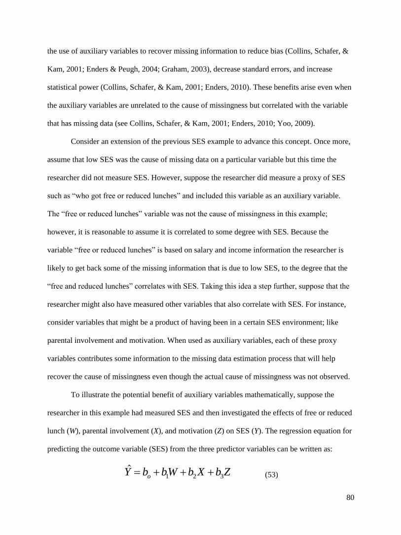
80

the use of auxiliary variables to recover missing information to reduce bias (Collins, Schafer, &

Kam, 2001; Enders & Peugh, 2004; Graham, 2003), decrease standard errors, and increase

statistical power (Collins, Schafer, & Kam, 2001; Enders, 2010). These benefits arise even when

the auxiliary variables are unrelated to the cause of missingness but correlated with the variable

that has missing data (see Collins, Schafer, & Kam, 2001; Enders, 2010; Yoo, 2009).

Consider an extension of the previous SES example to advance this concept. Once more,

assume that low SES was the cause of missing data on a particular variable but this time the

researcher did not measure SES. However, suppose the researcher did measure a proxy of SES

such as “who got free or reduced lunches” and included this variable as an auxiliary variable.

The “free or reduced lunches” variable was not the cause of missingness in this example;

however, it is reasonable to assume it is correlated to some degree with SES. Because the

variable “free or reduced lunches” is based on salary and income information the researcher is

likely to get back some of the missing information that is due to low SES, to the degree that the

“free and reduced lunches” correlates with SES. Taking this idea a step further, suppose that the

researcher might also have measured other variables that also correlate with SES. For instance,

consider variables that might be a product of having been in a certain SES environment; like

parental involvement and motivation. When used as auxiliary variables, each of these proxy

variables contributes some information to the missing data estimation process that will help

recover the cause of missingness even though the actual cause of missingness was not observed.

To illustrate the potential benefit of auxiliary variables mathematically, suppose the

researcher in this example had measured SES and then investigated the effects of free or reduced

lunch (W), parental involvement (X), and motivation (Z) on SES (Y). The regression equation for

predicting the outcome variable (SES) from the three predictor variables can be written as:

1 2 3ˆ

oY b bW b X b Z

(53)

81

where Y represents the predicted value of SES (Y), the b0 coefficient represents the intercept and

the b1, b2 , and b3 coefficients denote the linear relationship of free or reduced lunch, parental

involvement, and motivation to SES, respectively. Given this equation, assume that the

proportion of variance in the dependent variable (SES) which can be explained by the

independent variables (free or reduced lunch, parental involvement, and motivation) is

somewhere between a reasonable range of r2 = .30 - .40. This would indicate that 30 - 40% of the

variance in these three proxy auxiliary variables will help the researcher account for the MNAR

mechanism caused because SES was not actually measured. Given a large set of good auxiliary

variables, the research analyst may more reasonably assume the MAR assumption because the

missing data handling procedure is as informed as possible. Additionally, the resulting FMI

estimates are in theory lower than the percent missing. As Enders (2009) noted, the effectiveness

of auxiliary variables has been demonstrated even when the auxiliary variables, themselves,

contain relatively high levels of missing data.

Auxiliary variables for nonlinear causes of missingness. In practice, it is often the case

that complex causes of missing data are not adequately captured by additive linear regression

equations (Collins, Schafer, & Kam, 2001). Assume that missing data caused by low SES (from

the previous example) was actually caused by motivation as it relates to having been in a certain

SES environment and additionally parental involvement alleviates the effect of motivation on the

propensity of missing data. Therefore, while each individual’s level of motivation is negatively

related to his or her likelihood of having missing data, the strength of this relationship weakens

as the level of parental involvement increases. By including an interaction term between

motivation and parental involvement, the researcher can effectively remove bias from the

missing data handling procedure (Collins, et al., 2001; Schafer, 1997).

Typically, researchers assume linear relationships when using MI or FIML (Little and

Rubin, 2002); however, the inclusion of product terms or powered terms can add variables that

82

can approximate non-linear processes (Enders & Gottschall, 2011; Graham, 2009; Schafer,

1997). Therefore, missing data related to a non-linear function can be included in the missing

data handling process to explain why data are missing. As Enders and Gottschall (2011)

demonstrated, in some cases, knowledge of possible non-linear causes of missingness could be

important to satisfy the MAR assumption and lead to unbiased inferences. It seems reasonable

that a true all-inclusive strategy should incorporate interaction terms among the auxiliary

variables as well as polynomials to capture potentially useful non-linear information.

Auxiliary variable demonstration using simulated data. In order to demonstrate the bias

that can result when auxiliary variables are ignored during imputation, a series of Monte Carlo

simulations were conducted in line with those presented by Enders (2010). These simulations

intend to imitate a research scenario where it is of interest to estimate the mean vector and

covariance matrix between two variables, X and Y. These variables could be any combination of

continuous or categorical scales. Of current interest is the case where X and Y are bivariate

normally distributed continuous variables.

Now, suppose that Y is subject to nonresponse such that a monotone missing data pattern

is obtained. Figure 29 illustrates a diagram of this monotone missing data pattern where all

values of the variable X are observed and only some of the values of Y are observed. Notice that

in Figure 29 there are m cases of Y and p cases of X. There are numerous research situations that

lead to this pattern of missing data and it has been widely used in the literature to study missing

data (Enders, 2010; Little & Rubin, 2002). For instance, let Y represent a questionnaire item with

missing data and let X represent a demographic variable, like age, with no missing values. The

variable X could also represent a fixed variable controlled by the experimenter or any other

variable with complete data. This analysis model is certainly not comprehensive, but is sufficient

to show the potential effectiveness of auxiliary variables.

83

For simplicity, the manipulated factors only included: (a) magnitude of correlations

between the auxiliary variables and the variable with missingness, and (b) missing data

mechanism. The rate of missingness was fixed at 30% and the sample size was set to N = 100.

These factors were chosen due to their expected influence on the performance of missing data

handling procedures that incorporate auxiliary variables. For example, the effectiveness of

auxiliary variables is expected to improve as the magnitude of correlations increase given a

particular rate of missing and sample size (see Collins, Schafer, & Kam, 2001; Enders, 2010).

Additionally, the performance of auxiliary variables is expected to improve parameter estimation

even in a MNAR condition (in the absence of a missing data cause; see Enders, 2010). The

benefits of auxiliary variables are also considered in relation to non-linear MAR. Lastly, given a

MCAR condition, auxiliary variables do not influence bias but can instead demonstrate relative

improvements in power compared to the exclusion of auxiliary variables (Enders, 2010).

The following levels were selected: (a) magnitude of correlations (ρ = .10 to .80 by .10),

(b) missing data mechanism (MCAR, MAR, non-linear MAR, MNAR). For all variables the

means were set at µ = 0 and the variances were set at σ2 = 1.0. Results are expressed across the

range of correlations for each of the missing data mechanisms. The goal is to provide a clear

(though simplified) demonstration of auxiliary theory with simulated data. For each study, a

bivariate normal correlation model was used to generate population data for the associated

simulation studies. Figure 30 illustrates a path diagram of the population model including

auxiliary variables. Notice that the population correlation between the variables X and Y were

fixed at ρ = .30 for simplicity as were the associations between X and the three auxiliary

variables (Aux1 – Aux3). In contrast, the magnitude of associations between Y (the variable with

missingness) and the auxiliary variables range from .10 to .80 by .10.

Specifically, Mplus 6.0 (Muthén & Muthén, 1998–2010) was used to generate five

variables: X, Y, and three auxiliary variables (AUX1 – AUX3) in 1,000 multivariate normal data

84

sets of size 1,000 for each set of population values noted previously. After data generation, SAS

9.3 (SAS Institute Inc., 2011) was used to impose one of the four missing data mechanisms on Y.

After generating missingness, the data from all replications were analyzed with Mplus 6.0 where

the auxiliary variables were incorporated into the FIML estimation routine with the saturated

correlates model (see Graham, 2003).

Excluding a cause of missingness. For the first study, a MAR missing data pattern was

specified where missing data were generated by deleting 30% of the data in Y based on the lower

distribution of the first auxiliary variable (AUX1). This simulation was intended to show the

impact of excluding a cause of missingness (i.e., AUX1). That is, the missing data on Y are

MNAR because the cause of missingness was not included in the subsequent FIML procedure.

As illustrated in Table 4, the impact of omitting a cause of missingness depends on its

association with the incomplete variable (i.e., Y). Specifically, a negative bias is present that

increased as the relationship between the auxiliary variable and the variable with missingness

increased.

This relationship is depicted graphically in Figure 31, where the plotted line slopes down

and to the right demonstrating increasing negative bias. The direction of this bias directly relates

to the portion of AUX1 that was responsible for missingness and does not suggest a typical

direction for bias in relation to excluding a cause of missingness. Deleting 30% of the data in Y

based on the upper distribution of the first auxiliary variable (AUX1) would produce positive

bias. Because the missingness was entirely related to the omitted variable, including it in the

estimation process would result in unbiased estimates.

These findings support and replicate those described by Enders (2010). As he found,

“…omitting a correlate of missingness was not that detrimental when the correlation was weak

(e.g., r ≤ .30), but the estimates became increasingly biased as the correlation between the

auxiliary variable and the incomplete analysis variable increased in magnitude,” (p. 129). This

85

relationship explains the suggestion provided by Collins, Schafer, and Kam (2001) to locate

auxiliary variables that exceed an association of about r = .40 with the variables with missing

data.

Improving estimation with MNAR. For the second study, the data were generated as

previously noted except a MNAR missing data mechanism was specified where missing data

were generated by deleting 30% of the data in Y based on the lower distribution of the variable Y

itself. In this example, all three auxiliary variables (AUX1 – AUX3) are included in the FIML

estimation routine. This simulation was intended to show the ability of auxiliary variables to

improve parameter estimation even in a MNAR situation. The results of this simulation are

presented in Table 5 and Figure 32 and indicate auxiliary variables that are related to a variable

with missingness may reduce (through not eliminate) parameter bias. As before the performance

of auxiliary variables to reduce bias depended on the magnitude of the association between the

incomplete variable (i.e., Y) and the auxiliary variables. These findings support a similar

simulation by Enders (2010). He noted that under the MNAR condition, “although the average

parameter estimates did get closer to the true population values as the correlation increased, the

bias was still noticeable, even when the correlation between the auxiliary variable and the

missing analysis variable was 0.80,” (p. 130). As most researchers are unaware of all possible

causes of missingness, these findings encourage the use of auxiliary variables with strong

associations despite theoretical motivation for selecting auxiliary variables.

Including non-linear MAR. For the third study, a non-linear MAR mechanism was

generated by deleting 30% of the data in Y based on the lower distribution of an interaction term

between the first and second auxiliary variable (i.e., AUX1 × AUX2 = AUX12). The primary goal

of this simulation was to study parameter estimate bias when the cause of missingness was not a

linear process given that FIML assumes linear relationships among the analysis and auxiliary

variables.

86

To investigate this issue, two conditions are presented. First, the first two auxiliary

variables (AUX1 and AUX2) were included in the FIML estimation routine. This approach did not

contain the non-linear interaction term that actually caused missingness on Y; however, it did

include the linear components from which the interaction term was generated. Second, only the

newly created interaction term (AUX12) was included and the linear components were excluded.

This condition represents a lower bond on the effect of including a non-linear term as it used one

auxiliary variable rather than two (though the included term was theoretically more meaningful).

The results of this investigation are presented in Table 6 and demonstrate the greater bias

in the linear condition (first approach that included only AUX1 and AUX2) than in the non-linear

condition (the second condition that included only AUX12). Said differently, while the average

parameter estimates approached the true population values as the correlation among the auxiliary

variables and Y increased across both conditions, the bias was slightly more prevalent in the

linear only condition. These findings support prior work in the area of non-linear causes of

missingness (see Collins, Schafer & Kam, 2001) and demonstrate the viability for non-linear

auxiliary variable terms in FIML estimation. Further, these results present another problem as

including non-linear terms (i.e., interactions) preclude the inclusion of the accompanying linear

components because of estimation errors due to multicollinearity (see Graham, 2009 for

discussion of the resulting non-positive definite covariance matrix). A solution to this problem is

presented in an upcoming section where principal components are used to extract linear and non-

linear variance from auxiliary variables (as will be discussed principal components are, by

definition, uncorrelated).

Improving statistical power. For the last demonstration of the ability of auxiliary

variables to improve estimation, a MCAR missing data pattern was specified where missing data

were generated by deleting 30% of the data in Y based on a completely random process. Like the

previous simulations, this study was modeled after work by Enders (2010) and intended to

87

demonstrate the impact of auxiliary variables on statistical power. While the previous examples

generated biased parameter estimates by omitting the cause of missingness, this demonstration

did not because missingness was related to a completely random process where any value of Y

was as likely to be missing as any other value. Enders referred to this as a “benign” cause of

missingness; thus an assessment of bias in this situation is uninformative. Instead, this

investigation focused on estimates of statistical power relative to the association strength among

the variable with missingness and all three auxiliary variables.

The results of this simulation suggest that statistical power increases as the magnitude of

associations increase between the analysis variables with missingness and the auxiliary variables.

These findings are shown in Figure 33 where, for example, a correlation of r = .30 produces a

relative power value of 1.028, which suggests that the auxiliary variable increased power by

about 2.8%. Likewise, a correlation of r = .40 relates to a relative power value of about 4%. As

demonstrated in Figure 33 the relationship between power and association strength is non-linear

where the largest gains occur in power occur when the correlation exceeds about r = .40. This

finding further supports the suggestion of methodologists (e.g., Collins, Schafer, & Kam, 2001)

to choose auxiliary variables that are highly correlated with the outcome measures.

Auxiliary variable simulation summary. As demonstrated, auxiliary variables used in

conjunction FIML (or MI though not demonstrated here for clarity) are important tools for

researchers. Methodologists have generally endorsed an “inclusive strategy” with regard to

auxiliary variables, which recommends the generous use of all possible auxiliary variables from

a dataset rather than a “restrictive strategy” which incorporates a selected subset of auxiliary

variables (see Collins, Schafer, & Kam, 2001). As Collins, et al., note, the “inclusive strategy” is

recommended to reduce the chance of inadvertently omitting an important cause of missingness

while allowing for noticeable gains in terms of increased efficiency (e.g., power) and reduced

bias. The simulations presented explicitly demonstrate these ideas as they are important concepts

88

for the following discussion. While thus far little attention was given to the process of choosing

auxiliary variables aside from locating extra variables with strong associations, methodologists

have given considerable attention to the topic and the issue is relevant for the ensuing discussion.

Next, the topic of choosing auxiliary variables is elaborated on including rational for not always

selecting a few strongly correlated auxiliary variables.

Methods for choosing auxiliary variables. While the various sources of evidence

presented to this point provide a clear indication that the inclusion of auxiliary variables can have

an important impact on the results of any study with missing data, it is not clear what steps

should be taken to ensure that all important information relating to missing data are included in

the subsequent missing data handling procedure. Generally, it seems that the approaches taken to

choose auxiliary variables can be divided into two categories. The first approach (perhaps the

most popular approach; see Graham, Cumsille, & Shevock, in press) suggests that only a few

auxiliary variables (if any) are necessary to adequately satisfy the MAR assumption. Collins,

Shafer, and Kam (2001) refer to this approach as a “restrictive auxiliary variable strategy”. It is

clear that researchers utilizing this approach must assume that all relevant information is

included (Little & Rubin, 2002). Thus, from the restrictive strategy perspective, the researcher

must be comfortable with the assumption that any potential cause of missing data is explained by

the selected auxiliary variables.

The second approach begins with the assumption that results can vary with the auxiliary

variables chosen. Therefore, instead of focusing on a few influential auxiliary variables this

approach emphasizes a liberal use of auxiliary variables (see Collins, Shafer, & Kam, 2001). The

emphasis of this approach is on the incorporation of all possible information; which reduces the

chance of accidentally omitting an important cause of missingness. Collins, et al. refer to this

approach as an “inclusive auxiliary variable strategy”. This strategy suggests a way to conduct

research that is theoretically more in line with the MAR assumption because the researcher is

89

more likely to at least partially explain the cause of missingness through proxy variables (as

discussed previously). Thus, if the data set contains useful variables which are incorporated into

FIML or MI estimation process, the result should be an improvement in the quality of findings in

terms of noticeable gains in efficiency and reduced bias (see Collins, et al., 2001; Enders, 2010;

Enders, 2008).

Theoretically, the inclusive approach is superior to the restrictive strategy in that the

methodological literature notes there are no known dubious effects of including too many

auxiliary variables (e.g., Collins, Shafer, & Kam, 2001). As Collins, et al., note, “our results

indicate that far from being harmful, the inclusion of these variables is at worst neutral, and at

best extremely beneficial,” (p. 348). Though more work is needed to fully understand this topic

(i.e., simulations are based on specific conditions that may not generalize to practical

applications), the inclusive strategy seems preferable. Still, methodologists note that in practice it

is the restrictive approach that is typically used (see Enders, 2010; Graham, 2009). In order to

explain this discrepancy, the following section will further discuss the restrictive strategy and

review recommendations that methodologists make for choosing a restrictive set of auxiliary

variables.

Finding a few influential auxiliary variables. As Collins, Shafer, and Kam (2001) noted,

the approach that focuses on finding a small set of most relevant auxiliary variables is the most

common in part because this approach is favored by existing software and the associated

documentation because, “…neither of which encourages users to consider auxiliary variables or

informs them about how to incorporate them,” (p. 349). While progress has been made to revise

maximum likelihood-based programs (see the AUXILIARY (m) option in Mplus 6.0; Muthén &

Muthén, 1998–2010) and incorporate more informative documentation regarding the use of

auxiliary variables (see SAS Institute Inc., 2011), the restrictive strategy persists in the applied

literature. Therefore, it is important to consider how best to select influential auxiliary variables.

90

Enders (2010) acknowledged the inherent difficultly in establishing a rule of thumb for

selecting a particular set of auxiliary variables but discusses a few reasonable approaches beyond

simply looking for high correlations (though he does suggest this can be effective). He proposes

that researchers “maximize the squared correlation between the auxiliary variables and the

analysis model variables, and to do so with as few auxiliary variables as possible,” (p. 133). He

also suggests a related approach using an omnibus test for the missing completely at random

mechanism (Little’s MCAR test; see Little, 1998). If the data are not missing due strictly to a

random process, researchers can proceed to determine which specific variables contribute to

missingness (where complete and incomplete data groups are created for each variable). Then,

independent t-tests can be used to compare mean differences among potential auxiliary variables

(see Dixon, 1988 for details). Here, a significant difference suggests that cases with complete

data are different than cases with incomplete data on a given variable indicating the variable

should be included as an auxiliary variable. Lastly, Enders (2010), also suggests that a through

literature review should provide the researcher with ideas for important auxiliary variables to

include.

Some methodologists seem more comfortable providing rough guidelines for applied

researchers. For instance, Graham (2009) noted that, “adding auxiliary variables that are

correlated r = .50 or better with the variables of interest will generally help the analysis to have

less bias and more power,” (p. 565). This suggestion is supported by numerous simulation

studies and has become a sort of standard recommendation (recall Collins, Shafer, & Kam’s

similar recommendation). For instance, it is not uncommon for methodologists to define

auxiliary variables as, “…variables that are highly correlated with the analysis model variables,

but not necessarily part of the one’s analysis model,” (Graham, Cumsille, & Shevock, in press, p.

13). Regardless of the approach or number of auxiliary variables retained, the idea is to

91

acknowledge that the MAR assumption is not automatically met and a reasonable attempt should

be made to approximate it.

The appeal of a restrictive strategy. Assuming that the cause of missing data can be

captured by a few carefully selected variables, researchers can reach a point of “diminishing

returns” where only a few auxiliary variables contain useful information (Graham, Cumsille, &

Shevock, in press). In this situation the restrictive approach to auxiliary variables is preferable

because the addition of extra “junk” variables serves only to complicate the model (see Collins,

Shafer, & Kam, 2001).

Occasionally, modern missing data handling procedures fail to converge on a reliable,

acceptable solution (see Enders, 2002; 2010). These models tend to experience convergence

problems when there is insufficient data to estimate certain parameters (see Enders, 2010;

Graham, Cumsille, & Shevock, in press), or when there is a complex missing data pattern (see

Enders, 2010; Graham, 2009; Savalei & Bentler, 2009). Often these conditions arise when too

many variables are included in the data augmentation algorithm of MI or the iterative

optimization algorithm of FIML. For instance, Enders (2010) noted that when the number of

variables is greater than the number of cases, “…the data contain linear dependencies that cause

mathematical difficulties for regression-based imputation,” (p. 255). Asparouhov and Muthén

(2010) provide a useful example. Assume that a dataset contains 50 variables and N = 1000

participants. If the first variable of this dataset contains only 40 observations out of 1000 (i.e.,

960 missing values), the imputation model is not identified because 40 < 50 and the distribution

of parameters will fail to stabilize (i.e., not converge).

Non-convergence is not limited to situations when there are more cases than variables.

Enders and Bandalos (2001) studied convergence failure in FIML across a range of samples sizes

and missing data rates and found FIML to have a general (i.e., aggregated across all conditions)

non-convergence rate of approximately 10% with more problems associated with higher rates of

92

missing data and smaller samples sizes. In effect, as researchers include variables in MI or FIML

that contain high levels of missingness, the amount of missing data patterns can become

cumbersome and missing information can become too large to reconstruct given the observed

data (Enders, 2010; Enders & Bandalos, 2001; Savalei & Bentler, 2009). For instance, consider

that regression-based imputation procedures require separate regression equations for each

missing data pattern (Enders, 2010; Rubin, 1987).

Methodologists provide divergent guidelines regarding the best approach to “fix”

convergence failure. For instance, Schafer (1997) and Enders (2010) suggest adding an

informative ridge prior for MI. Enders described the use of a prior ridge as a technique that,

“…adds a small number of imaginary data records from a hypothetical population where the

variables are uncorrelated. These additional data points can stabilize estimation and eliminate

convergence problems, but they do so at the cost of introducing a slight bias to the simulated

parameter values (and thus the imputations),” (p. 256 – 257). Schafer provides a formula for

determining the value of the ridge prior when, “…either the data are sparse (e.g., n is

substantially larger than p), [where n is the number of cases and p is the number of variables] or

because such strong relationships exist among the variables that certain linear combinations of

the columns of Y (where Y is the complete data matrix comprising both observed and missing

observations) exhibit little or no variability,” (p. 155 – 156).

Other recommendations in the literature that apply to both MI and FIML include

increasing the number of iterations to an arbitrarily large value (e.g., Enders, 2010; Graham,

Cumsille, & Shevock, in press) or decreasing the convergence criteria (e.g., Asparouhov &

Muthén, 2010). Methodologists note that default convergence criteria and number of iterations

differ depending on the statistical software program used (e.g., Graham, 2009) and some

researchers consider any particular value to be relatively arbitrary (Van Buuren, Brand,

Groothuis-Oudshoorn, & Rubin, 2006).

93

Irrespective of these recommended fixes for non-convergence, a result may not be

produced or (perhaps less obvious for the researcher) an improper solution is generated. Consider

that decreasing the convergence criteria, for example, may result in missing value estimates that

are drawn from an instable posterior distribution (where parameter values change erratically

across iterations). Consequently, the practical recommendation in these situations has always

been to simply decreasing the number of auxiliary variables used (Enders, 2010). This point is

furthered by considering that in practice data may be robust to minor violations of the MAR

assumption (Collins, Schafer, & Kam, 2001). Also, methodologists often point out that a few

carefully selected auxiliary variables are generally enough (e.g., Enders, 2010; Graham,

Cumsille, & Shevock, in press). As Enders pointed out, “…my experience suggests that there is

little benefit to using a large number of auxiliary variables,” (p. 35). Thus the restrictive strategy

can be seen as more practical and efficient than the inclusive strategy.

Issues with the restrictive strategy. Given that there is a reason for missing data, it is

important to review the recommendations for selecting a restrictive set of auxiliary variables. To

begin with, it is typically not possible to prove that a particular variable (or set of variables) is

the sole cause of missingness. Consider that testing this assumption (that all variables responsible

for missing data are included) would require the missing values to be isolated from the influence

of all other possible causes (both observed and unobserved causes; see Enders, 2010). As

researchers are typically unaware of the precise causes of missing data, methodologists describe

this as “an ultimately untestable assumption,” (Baraldi & Enders, 2010; Enders, 2006; Peugh &

Enders, 2005; Schafer & Olsen, 1998). That is, researchers are unable to prove that any

particular set of auxiliary variables adequately capture the cause of missingness. Thus, the

assumption of a MAR process, which is required for unbiased FIML and MI estimation, becomes

a task for the research analyst, whom must assume that all influential variables are included in

the missing data handling procedure.

94

Recent research suggests that decisions regarding auxiliary variable selection are perhaps

more complex than they might seem (e.g., Kreuter & Olson, 2011; Little & Vartivarian, 2005).

The following discussion acknowledges that researchers do not always collect rich auxiliary

variables; and selecting variables based only on the strength of association may overshadow

important theoretical considerations relating to missingness. Further, it is reasonable to assume

that researchers accepting the restrictive strategy with regard to auxiliary variables may not

consider the ramifications related to rich auxiliary variables that are more likely of interest to

their inclusive strategy counterparts.

According to Kreuter and Olson (2011), it seems likely that the choice of auxiliary

variables for a particular study are often based on convenience (i.e., some extra correlated

variables in the data set that could be used) or tradition (i.e., a set of auxiliary variables were

used previously). Rarely is the choice of auxiliary variables justified by intentionally collecting

variables that are theoretically important to the response variables as well as to other key

variables that might also contain missingness (see Little & Vartivarian, 2005). That is, auxiliary

variables that correlate highly with outcome variables (i.e., Y’s) might not also relate highly to

predictor variables (i.e., X’s). Even in the case where there is strong theory and the researcher

has a deep understanding of the processes that might cause missing data, it seems unlikely that

such information would lead to the selection of a specific set of auxiliary variables that correlate

highly across all key analysis variables (i.e., Y’s and X’s; Kreuter and Olson, 2011).

Traditionally, the methodological literature does not seem to provide clear guidance

about theoretically relevant auxiliary variables or about situations where potential auxiliary

variables relate highly to some but not all analysis variables. Perhaps missing data research in the

social and behavioral sciences has not reached this level of sophistication. Still, if researchers

acknowledge that the choice of rich auxiliary variables is important to the subsequent statistical

95

inferences, then choosing auxiliary variables based on convenience or tradition may not be the

best approach.

A reasonable argument might even be made against many of the standard approaches for

selecting auxiliary variables. For instance, consider that the multiple t-test approach for selecting

auxiliary variables is based on mean differences and completely ignores covariance information

(Enders, 2010) which may hinder the researcher’s ability to effectively implement the restrictive

auxiliary variable strategy. In addition to this and other noted statistical limitations for accurately

choosing a specific set of auxiliary variables, the idea itself (that the research is able to find all

possible causes of missing data) is theoretically problematic. It is clear that a restrictive strategy

could lead researchers to face a dilemma regarding their results. The issue is that it is not clear if

the results are due to the relationships being studied or to the fact that a certain set of auxiliary

variables are chosen. Said differently, given the noted estimation improvements related to

auxiliary variables, it is possible for two researchers working on the same statistical model and

dataset to come to differing conclusions due to their particular use of auxiliary variables or for

the same researcher to obtain differing results based on which variables were selected from a

larger dataset. This situation led Enders (2010) to recommend that the researcher responsible for

handling missing data be the same researcher responsible for analyzing the data.

Additionally, reducing the number of variables used in MI and FIML due to estimation

failure is at odds with current recommendations in favor of an inclusive strategy with regard to

auxiliary variables (i.e., the inclusion of all possible causes or correlates of missingness into the

missing data estimation routine). Large data projects can present a particular challenge to

software convergence because it is possible to have hundreds of potential auxiliary variables to

inform the missing data estimation procedure. As Graham, et al. (in press) note, “…there is an

upper limit on how many auxiliary variables can feasibly be included in the model, (p. 32). This

96

situation is compounded when the researcher incorporates non-linear information (e.g., powered

terms and interactions), especially when the auxiliary variables also have missing data.

It is clear that auxiliary variables are important tools for theoretically approximating the

MAR assumption and practically for improving parameter estimates by decreasing standard

errors and increasing statistical power. Further, methodologists typically recommend an inclusive

strategy concerning auxiliary variables and seem to suggest a restrictive strategy as a practical

approach given current software limitations (Enders, 2010). As Collins, Schafer & Kam (2001)

stated, “we wish to stress that this [the restricted use of auxiliary variables] has nothing to do

with statistical theory,” (p. 349). They describe only benefits from including as many auxiliary

variables as possible and note that the limitation is with software and the associated

documentation.

The literature does not provide clear guidance for selecting an appropriate subset of

auxiliary variables. Thus, the researcher is faced with a challenge regarding the known benefits

of auxiliary variables and the practical limitations of current statistical software. Currently,

methodologists recommend a solution that involves selecting a few good auxiliary variables that

correlate highly with the analysis variables (e.g., Collins, Schafer, & Kam, 2001; Enders, 2010;

Graham, 2009). However, simulation studies regarding auxiliary variables have typically not

considered some of the complexities that may exist (e.g., non-linear information; see Enders &

Gottschall, 2011). That is, selecting a few auxiliary variables that correlate most highly with the

outcome measures may be effective in some situations, but is not likely the best approach in

others. Therefore, it is reasonable to question the plausibility of MAR when a restrictive strategy

is incorporated via MI or FIML. Specifically, the degree to which a set of auxiliary variables

influence parameter estimates in relation to all possible auxiliary variables is unclear and

ultimately depends on the cause of missingness, which is unknown.

97

A practical all-inclusive auxiliary variable strategy. While there will always be

uncertainty regarding the cause of missing data, it is a theoretically more reasonable

approximation of the MAR assumption to reveal and incorporate as many potential causes of

missingness as possible (including non-linear information). Therefore, I propose a practical

solution where auxiliary variables are viewed as a collection of potentially useful variance rather

than as specific variables that correlate with the analysis variables.

The use of methods to consolidate large numbers of variables and incorporate non-linear

information (such as interaction terms and power terms) have come of age elsewhere in the

social and behavioral sciences, and need to be incorporated more routinely into modern missing

data handling procedures. Consequently, the following approach focuses on a method of using

principal component analysis (PCA) to obtain auxiliary variables to inform missing data

handling procedures. Specifically, PCA is used to reduce the dimensionality of all possible

auxiliary variables in a data set. A new smaller set of auxiliary variables are created (e.g.,

principal components) that contain all the useful information (both linear and non-linear) from

the original dataset. These new uncorrelated principal component variables are then used as

auxiliary variables in an “all-inclusive” approach to best inform missing data handling

procedure.

The missing data literature has recognized that there will always be uncertainty regarding

the cause of missing data; however, the literature’s practice of encouraging the restrictive

strategy may not emphasize enough that the MAR assumption is not automatically met. In theory

it is a more reasonable approximation of the MAR assumption (i.e., the research analyst must

assume that all influential variables are included in the missing data handling procedure) to

incorporate all potential causes of missingness by extracting variance information that would

otherwise remain hidden within the data. These relationships can be important and may lead

researchers to more informed inferences.

98

In order to present the PCA auxiliary variable approach, discussion now turns elsewhere

in the social and behavioral sciences (beyond the typical missing data literature) to PCA a known

method for extracting useful linear and non-linear variance information and condensing that

information into a smaller subset of variables. To this end, PCA is introduced in the following

section followed by an introductory to how variance can be effectively extracted from observed

variables and used for other multivariate analytic techniques, like MI and FIML.

An Introduction to Principal Components Analysis

In the social and behavioral sciences, researchers are frequently interested in obtaining

information from participants across a large collection of variables. Fundamentally, Principal

Components Analysis (PCA) is a multivariate data reduction technique that involves the linear

transformation of a large set of variables into a new, more parsimonious set of variables (i.e., the

principal components) that are uncorrelated and that contain most of the original information

(Dunteman, 1989; Jackson, 1991; Joliffe, 2002). In this way, PCA is used to explain (through

linear combinations) the variance-covariance structure of a set of variables, (Johnson & Wichern,

2002). While the covariance information informs the data reduction process (i.e., highly

correlated variables can be combined because they share information), the method of PCA is

based on variances (Joliffe, 2002; Preacher, MacCallum, 2003; Widaman, 2007). That is, PCA

does not attempt to explain the covariance information; rather PCA depends directly on the

variances. The central idea of PCA is to find (through some form of eigendecomposition) a set of

k principal components ( 1 2componet ,componet ,...,componetk ) that contain as much information

(i.e., variance) as possible from the original p variables ( 1 2var , var ,..., varp ), where k < p. The k

principal components contain most of the important information from the p original variables

and can then replace them in further analyses (Johnson & Wichern, 2002; Joliffe, 2002).

99

Consequently, the original data set is reduced from n measurements on p variables to n

measurements of k variables (see Figure 37).

Geometrically, PCA is carried out by projecting the original data on a smaller number of

dimensions, which are specifically chosen to take advantage of the variance of the variables

(Jackson, 1991; Wickens, 1995). A useful metaphor is provided by photography. Consider that a

photograph is a 2-dimensional representation of a 3-dimensional object. The object in the

picture, depending on the angle (i.e., rotation), is recognizable because it contains most of the

original information. In other words, the third dimension is not necessary to identify the object in

the picture, so it can be collapsed without losing important information. The process of

projection will be illustrated mathematically in the forthcoming discussion.

An idea frequently advanced in favor of PCA is its potential to reveal variable

relationships by extracting variance information that would otherwise remain hidden (see

Johnson & Wichern, 2002). These relationships can be important and lead researchers to novel

interpretations of the data (Johnson & Wichern, 2002). Although many applications of PCA have

been developed (see Jackson, 1991; Joliffe, 2002), the common designs within the social

sciences include: errantly using PCA as a variant of factor analysis (see Widaman, 2007) and

using PCA as a preliminary step for other statistical techniques like multiple regression, and

cluster analysis (Jackson, 1991; Johnson & Wichern, 2002; Joliffe, 2002).

The Historical Context of Principle Component Analysis

In 1901, Karl Pearson introduced “the method of principal axes”, an idea that is regarded

as the earliest version of principal components analysis (Cowles, 2001; Dunteman, 1989;

Jackson, 1991; Joliffe, 2002). His article titled, “On Lines and Planes of Closest Fit to Systems

of Points in Space,” illustrates a combination of quantitative methodology relating to statistical

variance with the geometrical and graphical method of moments from mechanics (see Aldrich,

2007; Pearson, 1936; Porter, 2004). It provides a theoretical motivation and the statistical

100

groundwork for explaining the sample variance among a set of p variables and in doing so

outlines the best fitting lines and planes (i.e., principal components) to a p-dimensional scatter

plot. Pearson introduced an important statistical tool for data reduction, which was later

described (and independently developed) by Hotelling (1933) as a “principal components

analysis” (see Cowles, 2001).

Pearson’s work on “best fitting lines and planes” was a substantial achievement at the

time, especially considering the context from which it developed in the early 20th

century. The

fundamental concepts leading to the development of principal components analysis can be traced

as far back as the work of Leonhard Euler in the late-18th

century. Euler introduced the idea of

principal axis rotation and described it mathematically by the angles that the rotated axes make

relative to the original coordinate position (see Anderson, 1830). Later, Joseph-Lewis Lagrange

studied principal axis rotation, based on earlier work by Euler (see Anderson, 1830), and

introduced orthogonal transformations (Hawkins, 1975). He also made the connection that a

quadratic form can be reduced to its sum of square terms by solving the corresponding

eigenvalue problem (e.g., using Lagrange multipliers). Specifically, the resulting eigenvectors

are the direction cosines (i.e., angles) of the rotated axes relative to the original axis position in

3-dimensional space (Hawkins, 1974). This work was included in Lagrange’s influential 1788

publication, Mécanique Analytique, (analytical mechanics).

As Hawkins (1974) notes, Lagrange’s orthogonal transformation technique depends on

“the reality of the eigenvalues,” (p. 564) and Lagrange only proved that eigenvalues were real in,

“a case of the cubic” (i.e., 3-dimensional space). This limitation was overcome in the early 19th

century when Augustin-Louis Cauchy used his theory of determinates to extend Langrage’s

principal axis theorem from three dimensions to p-dimensional space (Hawkins, 1974). That is,

he proved that real eigenvalues could be derived from a symmetric matrix of any given size.

Throughout the 19th

century, other significant developments took place including further work on

101

eigenvalue decomposition (such as the development of singular value decomposition; see Joliffe,

2002) and the publication in 1888 of Galton’s, Co-relations and Their Measurement, Chiefly

from Anthropometric Data, which introduced regression and correlation (see Cowles, 2001).

During the same time that Galton was describing correlation and regression, Karl Pearson

was teaching mechanics to engineering students (among other courses) while working as a

professor of applied mathematics at the University College London (see Aldrich, 2007; Porter,

2004). While referring to Pearson’s use of “graphical statics” in these lectures, Aldrich describes

that, “Pearson’s earliest work on probability was not linked to his graphical projects; it was

essentially philosophical but it was linked to mechanics because his philosophical projects came

out of mechanics,” (p. 5). In 1891, Pearson added courses on the geometry of motion and the

graphical representation of statistics (Aldrich, 2007). Two years later, Pearson developed his

“methods of moments” which borrowed heavily from mechanics, especially in relation to

graphical statics (Aldrich, 2007).

By the beginning of the 20th

century, Pearson was in a fitting position to develop his

version of principal components analysis. In Pearson’s 1901 paper, he began by describing that

the best fitting regression line for a variable y given the value of another variable x is not the

same as the best fitting regression line for x given a particular value of y. Essentially, a different

line of best fit is obtained depending on which variable is designated as the dependent variable.

Therefore, he defined a line (or plane) of best fit that minimizes the sum of squared errors from

each point in a p-dimensional scatter plot to the best fitting line itself (i.e., the principal

component). Intuitively, the line (or plane) of best fit for a set of p correlated variables

transforms the data by rotating the original coordinate axes or vectors about their centroids (i.e.,

means). The axes are rotated so that they go through the clusters of points in a fashion that

minimizes the sum of squared errors.

102

Consider a brief example to illustrate the concept. In this example, two random normal

variables (x and y) have been generated on 25 observations with a mean of zero and a correlation

of .869. Geometrically, each p variable represents an axis in p dimensional space. Variables that

share variance (i.e., are highly correlated) create tighter clusters of points than variables that are

not related. These data are displayed in Table 7 and will be referenced throughout the discussion

of principal components analysis for didactic purposes. Figure 38 illustrates a scatterplot of these

data with a superimposed correlation ellipse and fitted lines.

Notice that in Figure 38 the regression of variable x on y and of variable y on x produces

different regression lines. Also notice that the lines of best and worst fit for the two variables x

and y are perpendicular but rotated from the original coordinate positions. As Pearson (1901)

described, the best fitting line (or plane) for a series of points in p-dimensional space,

“…coincides in direction with the maximum axis of the correlation ellipsoid, and the mean

square residual,” (see Pearson, p. 565).

Figure 39 provides a plot of the transformed data. That is, the principal axes have been

rotated to minimize the sum of squared errors perpendicular to the line of best fit. The locations

of the new axes define the new variables (i.e., the principal components) which are weighted

according to the amount of total variance that they describe and are oriented in “…a direction of

uncorrelated variation,” (Pearson, 1901, p. 566).

Recall that the variables x and y are highly correlated (i.e., r = .869) so they share

variation. The degree of overlap between these two variables directly relates to the amount of

variance explained by the best and worst fitting line. Said differently, Figure 39 illustrates that

the first principal component (i.e., the line of best fit) explains the greatest amount of variance

while the second principal component (i.e., the line of worst fit) explains the residual variance

not already explained. Consider that if the variables x and y were uncorrelated (i.e., a spherical

cloud of points), the principal components would essentially explain the same amount of

103

variation and any transformation of the data would not result in a dimensional reduction of the

data.

The next major advancement in the development of PCA came in 1933 with the

publication of Harold Hotelling’s paper, Analysis of a Complex of Statistical Variables into

Principal Components, which described principal components analysis essentially as we know it

today. Rather than approaching principal components from a geometric perspective, Hotelling

derived principal components algebraically using Lagrange Multipliers to solve the

characteristic equation (i.e., an eigenvalue and eigenvector problem; see Jackson, 1991). Cowles

(2001) notes that there is no reason to think that Hotelling was influenced in any way by

Pearson’s work, which was published nearly 30 years prior.

My assumption is that Hotelling, like Pearson, was initially influenced by analytic

geometry. I base this assumption on the fact that in addition to scalar algebra Hotelling also

introduced a “curious” notational convention from tensor calculus (i.e., geometrical vector

calculus; see Bock, 2007). As Bock notes, “surely, this is the only paper containing tensor

notation in the entire psychological literature and perhaps the statistical literature,” (p. 42).

Hotelling also provides a brief geometric explanation of principal components (e.g., axis

rotation) in his 1933 paper, which differs from Pearson’s earlier description but illustrates that he

was aware of a geometric interpretation of principal components. Regardless of the reason for

Hotelling’s unique notation or the initial inspiration for the method, he developed the idea of

principal components analysis heavily from a factor analytic perspective (Bock, 2007; Cowles,

2001; Jolliffe, 2002).

Much of the confusion that currently exists in the social sciences between factor analysis

and principal components analysis may derive from Hotelling’s 1933 paper. In this paper

Hotelling writes, “it is natural to ask whether some more fundamental set of independent

variables exist, perhaps fewer in number than the x’s, which determine the values the x’s will

104

take,” (p. 417, emphasis is mine). Unfortunately, this language is misleading because principal

components as Hotelling described them (and as they are currently understood) are

mathematically determined by linear combinations of the x’s. That is, the x’s cause “the

fundamental set of independent variables” rather than the other way around. Furthermore, the

equations underlying these methods are quite different (see Joliffe, 2002; Widaman, 2007).

It is interesting that Hotelling does not explicitly distinguish his method from factor

analysis. For instance, when naming his transformed variables Hotelling noted that the word

“factor” was used in psychology to describe a similar procedure but the word “component” was

most appropriate due to, “…conflicting word usage attaching to the word “factor” in

mathematics” and “…in view of the prospect of application of these ideas outside of

psychology,” (p. 417). In fact, as Joliffe (2002) notes, much of Hotelling’s paper seems to deal

with factor analysis rather than principal components analysis. Actually, Bock (2007) suggests

that a misunderstanding of the fundamental differences between the method of factor analysis

and that of principal components analysis (by Hotelling) created “antagonism” between

Hotelling and L.L. Thurstone, a colleague of Hotelling and an essential figure in the

development of factor analysis. For a more complete discussion of the relationship between

factor analysis (FA) and principal component analysis, see Widaman (2007).

Defining Principal Components Analysis

When a researcher collects data each variable usually contains a certain amount of

variance (i.e., the distribution about the mean response). The sample covariance matrix (S)

provides a representation of the covariation between each variable in the sample and can be

represented as:

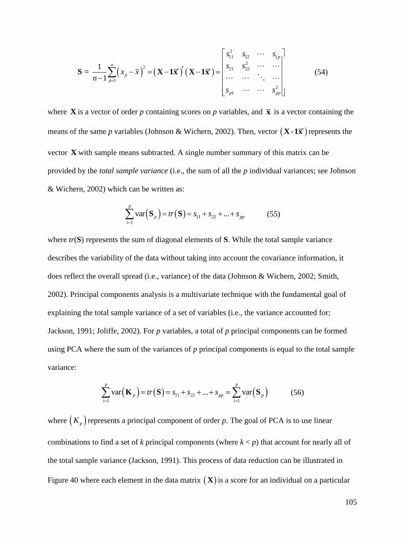
105

2

11 12 1

22 21 22

1

2

1

1 =

1

p

n

p

p

p pp

s s s

s sx x

n

s s

S X 1x X 1x (54)

where X is a vector of order p containing scores on p variables, and x is a vector containing the

means of the same p variables (Johnson & Wichern, 2002). Then, vector X -1x represents the

vector X with sample means subtracted. A single number summary of this matrix can be

provided by the total sample variance (i.e., the sum of all the p individual variances; see Johnson

& Wichern, 2002) which can be written as:

11 22

1

var ...p

p pp

i

tr s s s

S S (55)

where tr(S) represents the sum of diagonal elements of S. While the total sample variance

describes the variability of the data without taking into account the covariance information, it

does reflect the overall spread (i.e., variance) of the data (Johnson & Wichern, 2002; Smith,

2002). Principal components analysis is a multivariate technique with the fundamental goal of

explaining the total sample variance of a set of variables (i.e., the variance accounted for;

Jackson, 1991; Joliffe, 2002). For p variables, a total of p principal components can be formed

using PCA where the sum of the variances of p principal components is equal to the total sample

variance:

11 22

1 1

var ... varp p

p pp p

i i

tr s s s

K S S (56)

where pK represents a principal component of order p. The goal of PCA is to use linear

combinations to find a set of k principal components (where k < p) that account for nearly all of

the total sample variance (Jackson, 1991). This process of data reduction can be illustrated in

Figure 40 where each element in the data matrix X is a score for an individual on a particular

106

variable. Note that in Figure 40 ipx is the score for the ith

individual on the pth

variable. Likewise,

each element in the principal components matrix ( K ) is a score for an individual on a particular

component. Therefore, ipk is the score for the ith

individual on the kth

component. Another

important aspect of Figure 40 is that the original data matrix is transformed into a matrix of

principal components through the use of a covariance or correlation matrix. The

covariance/correlation matrix is used to derive the fundamental mathematics behind principal

components analysis. These fundamental aspects of PCA relate to the weighting of linear

combinations of variables and will be mathematically illustrated in the following section.

In the social sciences, linear combinations are often used to form composites scores

(Johnson & Wichern, 2002). For instance, a composite score might be formed as a linear

combination (e.g., summation) of a set of items that measure a particular construct, which can be

written as:

1 1 2 2 ...k k k kp pC a x a x a x (57)

where px represents each of the p items, kpa represents a weight (e.g., 0, 1) associated with each of

the k composite scores on each of the p items, and kC indicates a composite score that is expected

to contain all the important variance in the original p items.

Similarly, principal components are created from linear combinations of items that

combine variance; however, the weights (e.g., pka ) are derived mathematically to maximize the

amount of variance that can be explained by each of the p composite scores (Dunteman, 1989).

For example, letting K represent a vector of the new composite variables (i.e., principal

components) the linear combinations for PCA can be written as: K a Xor more descriptively

as:

107

1 11 1 12 2 1

2 21 1 22 2 2

1 1 2 2

...

...

...

p p

p p

p p p pp p

K a X a X a X

K a X a X a X

K a X a X a X

1

2

p

a X

a X

a X

(58)

where pX represents each of the original p variables and ppa represents a weight coefficient that

maximizes the variance in the linear composite (see Jackson, 1991). Thus, this equation

represents a set of linear equations, one for each component in K. Each equation represents a

composite variable in K as a linear combination of the variables in X. For instance, the variance

of the first principal component (K1) is as large as possible given the restriction that the sum of

the squared weight coefficients equal 1.0:

2 2 2

1 11 12 1... 1pK a a a (59)

This constraint (i.e., the “normalization” constraint) is imposed on the weight coefficients for a

particular principal component (e.g., K1) to prevent an arbitrary increase in the weights during

the variance maximization process (via Lagrange multipliers), which would arbitrarily inflate the

maximum variance of that principal component (Jackson, 1991; Joliffe, 2002). Essentially,

Lagrange multipliers locate the maximum (or minimum) value of an estimate that is subject to

certain constraints (Hotelling, 1933; Joliffe, 2002). A practical illustration for the way a

Lagrange multiplier operates is provided by excise taxes. Excise taxes are special taxes on

particular products and can be used to limit a particular behavior. For instance, a large excise tax

on cigarettes is commonly used to limit the use of the product. Consider that this tax effectively

constrains the maximum cigarettes consumed by a person. Likewise, Lagrange multipliers can be

used to estimate a maximum value given a particular constraint. The constraint prevents the

maximum value from unrestricted increases. Regarding PCA the constraint is that the sum of

these squared weight coefficients are set to 1.0 (note that other restrictions are possible but

typically not desirable; see Jackson, 1991). This allows the relative weight estimates to be

108

meaningful and reflect each variables contribution to the total variance of a particular principal

component (e.g., K1). The variance of the second principal component (K2) is as large as possible

given the variance not already captured by K1 and is also subject to the constraint that the sum of

its weights equal 1.0:

2 2 2

2 21 22 2... 1pK a a a (60)

Because the second principal component does not use variance that was already assumed by the

first principal component, the components do not share variance, so the covariance (or

correlation) among the first two principal components is zero:

1 2, 0Cov K K (61)

Likewise, the variance of the pth

principal component (Kp) is as large as possible given the

variance not already assumed by Kp-1 and subject to the constraints that

2 2 2

1 2 ... 1p p ppa a a (62)

Similarly, the covariance among any principal components (e.g., i and j) is zero:

, 0i jCov K K (63)

Further, the variance (i.e., var) of each successive component pK is smaller than the previous

component such that:

1 2var var ... var pK K K (64)

The key to deriving principal components algebraically is solving the characteristic

equation, a fundamental outcome of matrix algebra where a square positive-definite matrix (e.g.,

S) can be mathematically decomposed into a smaller set of foundational variance (i.e.,

eigenvalues and eigenvectors; Jackson, 1991; Joliffe, 2002; Kolman, 1996). More specifically,

the weight coefficients (i.e., ppa ) are derived from an eigenvector of matrix S corresponding to

the pth

largest eigenvalue. Eigenvectors are effectively the mechanics behind the estimation of

109

principal components (see Equation 11). The fundamental role of eigenvectors in relation to a

covariance matrix is a key concept in PCA and is therefore demonstrated in the next section. The

process of solving the characteristic equation to determine the weight coefficients (i.e.,

eigenvectors) used in PCA will be described mathematically in the following section. The

following discussion presents the basic ideas behind finding principal components through the

eigenvalues and eigenvectors and is intended for didactic purposes. In practice, statistical

programs are used to calculate principal components via a number of possible algorithms. As

Joliffe (2002) noted, analysts interested in the last few principal components may find

differences across algorithms and should consider the approach taken by the specific software

program of interest. As the subsequent discussion of PCA in relation to auxiliary variables does

not require the last few components, this topic is not addressed. Interested readers should see

Joliffee (2002, p. 408 – 414) for discussion.

Eigenvectors. A vector is a matrix with a single column (column vector) or a single row

(row vector). A vector can be thought of as a line (with a direction) emanating from the origin

and terminating at a point. For instance, take the column vector:

1

0.77

0.64

u (65)

which is a trajectory in 2 dimensional space that represents an arrow pointing from the origin (0,

0) to a point (0.77, 0.64). The vector 1u is illustrated in Figure 41.

An eigenvector is a specific type of vector. The word “eigen” is a German word meaning

“proper” or “characteristic” (see Kolman, 1996). An eigenvector is a vector that has a “proper”

(i.e., fundamental) relationship with a particular symmetric matrix which can be determined

using matrix algebra (Johnson & Wichern, 2002; Kolman, 1996; Wickens, 1995). To illustrate,

consider the sample covariance matrix (S) from the simulated data in Table 7:

110

11 21

12 22

0.95 0.71

0.71 0.67

s s

s s

S (66)

There are p = 2 variables in this covariance matrix. Matrix algebra provides a mathematical

framework for manipulating matrices and vectors in a way that identifies eigenvectors (Abdi &

Williams, 2010; Jackson, 1991; Smith, 2002). For instance, when S is post multiplied by the

vector 1u , the result is another vector 1.1u :

0.95 0.71 0.77 1.18

0.71 0.67 0.64 0.97

(67)

The “characteristic” of this new vector is that it is 1.53 times the original vector:

1.18 0.77

1.530.97 0.64

(68)

That is, the scalar multiplication of vector 1u (i.e., the multiplication of a single number by a

vector) results in changing the length of the vector but not the angle of the vector (see Johnson &

Wichern, 2002; Kolman, 1996), which is illustrated in Figure 42 where the new vector 1.1u is

plotted as an extension (a lengthening) of the original vector 1u . As noted previously, the

difference in length between 1u and 1.1u is determined by a particular scalar that defines the

relationship of the original vector and the covariance matrix. In other words, the covariance

matrix maps 1u onto a scalar (i.e., 1.53) multiple of itself, (Kolman, 1996). Therefore, 1u is a

“basis vector” or eigenvector of the square matrix S (see Johnson & Wichern, 2002). The scalar

(i.e., 1.53) is known as an eigenvalue. Regardless of the length of 1u the associated eigenvalue

defined by the covariance matrix is constant. That is, multiplying the vector 1u by some value

(e.g., 5) would produce:

111

0.77 3.865

0.64 3.18

0.95 0.71 3.86 5.92

0.71 0.67 3.18 4.87

5.92 3.861.53

4.87 3.18

(69)

with a 1u and 1.1u vector that are 5 times longer than before but that have the same relative length

of 1.53. The length of a vector does not change the basis for the relationship among the

eigenvector and the covariance matrix.

A covariance matrix of order p has p eigenvectors which are all orthogonal to each other

(i.e., Joliffe, 2002; Kolman, 1996). Each eigenvector provides a new reference point (rather than

the original coordinate axes) for interpreting data in p dimensional space (Johnson & Wichern,

2002). Consider the p = 2 eigenvectors associated with the sample covariance matrix S in the

following illustration (see Figure 43) where 1u represents the eigenvector for the first dimension

and 2u represents the eigenvector for the second dimension, which is:

0.64

0.77

2u (70)

Notice that the vectors 1u and 2u appear to be orthogonal (i.e., perpendicular). The inner product

of two vectors 1u and 2u is the sum of element-by-element multiplication (see Johnson &

Wichern, 2002):

11 21 12 22 ... pp ppu u u u u u 1 2u u (71)

For instance given the vectors 1u and 2u the inner product can be calculated as:

112

1

1 2

0.77 0.64,

0.64 0.77

0.640.77 0.64

0.77

0.77* 0.64 0.64*0.77 0

2u u

u u (72)

The inner product is used to compute the angle between vectors (Johnson & Wichern, 2002;

Kolman, 1996). For instance, the angle between two vectors 1u and 2u is the cos where:

1 2

1 1 2 2*

u u

u u u u

(73)

From the current example,

1 2

1 1 2 2

1

0cos 0

1* 1*

cos 0 90o

u u

u u u u (74)

Thus it can be illustrated that the eigenvectors 1u and 2u are in fact orthogonal because their inner

product is zero (i.e., 0 1 2u u ) which indicates the angle between these vectors is 90o as is

illustrated in Figure 44.

While the vector 2u in Figure 44 may seem to be longer than the vector 1u , they are

exactly the same length. The length of a particular vector emanating from the origin is given by

the Pythagorean formula (see Johnson & Wichern, 2002). For instance letting Lu represent the

length of a particular vector:

2 2 2

1 2 ... pL u u u u u u (75)

While the length of a particular eigenvector is not particularly relevant (as illustrated in Equation

22), the relative length of an eigenvector in relation to the length of another eigenvector is

meaningful when the eigenvectors are used as reference points for interpreting data (Jackson,

113

1991). To standardize these reference points, the length of each p eigenvectors are set equal to

one. That is, if u u = 1 (i.e., the sum of squares of elements of u is equal to 1) then u is said to

be a standardized eigenvector of S (see Jackson, 1991). Standardized eigenvectors may be

obtained by a simple transformation of the eigenvector:

1

u

u u (76)

For instance, the standardized length of the vector 1u is:

2 2

0.77 0.7711.0

0.64 0.640.77 0.64

(77)

which, in the current example, is the same length as the original vector. Typically, this is not the

case; however, the current data (see Table 7) were simulated to have a mean of 0 and a variance

of 1.0; therefore, the eigenvectors 1u and 2u are effectively already standardized.

As Joliffe (2002) notes, occasionally researchers refer to the standardized eigenvectors as

“principal components” even though, this practice is not technically accurate and leads to

confusion. Rather, “it is preferable to reserve the term “principal components” for the derived

variables pa X , and refer to pa as the vector of coefficients or loadings for the pth PC,” (p. 6).

This point is further developed in the following section.

Finding eigenvectors. Assuming In the previous section, the eigenvectors of the example

covariance matrix S were provided as:

2

0.77 0.64

0.64 0.77

1u u u (78)

In practice, matrix algebra is needed to uncover the eigenvectors associated with S. The

following section introduces eigendecomposition (reduction of the covariance matrix to its

characteristic roots and vectors) by Lagrange multipliers (see Jackson, 1991) using the data in

Table 7. Essentially, Lagrange multipliers locate the maximum (or minimum) of a linear function

114

that is subject to certain constraints (Hotelling, 1933; Joliffe, 2002). As will soon be illustrated,

Lagrange multipliers are used to maximize pa X subject to the constraint that

2 2 2

1 2 ... 1p p ppa a a . While these illustrations involve only two variables these concepts

generalize to p variables.

To begin, consider a sample covariance matrix (S) of order p. If u is a column vector of

order p, and is a scalar such that Su u , then 1 2, ,..., p is said to be an eigenvalue (or

characteristic root) of S and u 1 2, ,..., pu u u is said to be the corresponding eigenvector (or

characteristic vector) of S (Johnson & Wichern, 2002; Jackson, 1991). This expression can be

illustrated in expanded form as:

11 1 12 2 1 1

21 1 22 2 2 2

1 1 2 2

...

...

...

p p

p p

p p pp p p

s u s u s u u

s u s u s u u

s u s u s u u

(79)

Determining the eigenvalues and eigenvectors in this formula is known as solving a classical

eigenproblem (see Joliffe, 2002; Voelz, 2006). The equation Su u can be rearranged into a

homogeneous form (i.e., setting the right side of the equation equal to zero) known as the

characteristic equation, which can be written as (see Jackson, 1991):

0 S I (80)

where I is an identity matrix of order p. This equation derives p eigenvalues that can be ordered

in sequence from largest to smallest (i.e., 1 2 p ). Consider the following illustration of

the characteristic equation to solve for the eigenvalues of the example covariance matrix S (see

Jackson, 1991):

115

2

2

0det det det

0

4

2 2

a b

c d

a b a b

c d c d

a d bc

bc a da da d ad bc

S

S I (81)

Notice that the matrix algebra produces a quadratic equation that is solved by factoring. To

further illustrate the derivation of eigenvalues, let the covariance matrix S be defined by the

simulated data in Table 7, the sample covariance matrix is:

11 21

12 22

0.95 0.71

0.71 0.67

s s

s s

S (82)

There are p = 2 variables in this covariance matrix. Applying S to the characteristic equation

produces:

2

2

0.95 0.71 0 0.95 0.71

0.71 0.67 0 0.71 0.67

0.95 0.71det 0.95 0.67 0.71*0.71

0.71 0.67

0.95 0.67 0.95*0.67 0.71*0.71

4*0.71*0.71 0.95 0.670.95 0.67

2 2

1.533,0

S I

.086

(83)

where the eigenvalues are 1 1.533 and 2 0.086 . These eigenvalues represent the variance of

the p = 2 principal components with the first component 1 explaining most of the variance.

Now that the eigenvalues are determined, the associated eigenvectors can be calculated by

applying the sample covariance matrix S to the following equations (see Jackson, 1991):

0 S I u (84)

and the normalizing equation:

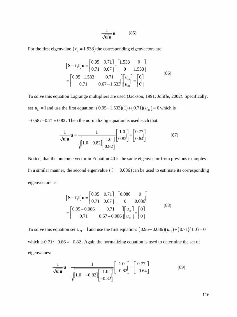
116

1

u

u u (85)

For the first eigenvalue 1 1.533 the corresponding eigenvectors are:

1

11

21

0.95 0.71 1.533 0

0.71 0.67 0 1.533

0.95 1.533 0.71 0

0.71 0.67 1.533 0

u

u

S I u

(86)

To solve this equation Lagrange multipliers are used (Jackson, 1991; Joliffe, 2002). Specifically,

set 11 1u and use the first equation: 210.95 1.533 1 0.71 0u which is

0.58 / 0.71 0.82 . Then the normalizing equation is used such that:

1.0 0.771 1

0.82 0.641.01.0 0.82

0.82

uu u

(87)

Notice, that the outcome vector in Equation 40 is the same eigenvector from previous examples.

In a similar manner, the second eigenvalue 1 0.086 can be used to estimate its corresponding

eigenvectors as:

1

11

21

0.95 0.71 0.086 0

0.71 0.67 0 0.086

0.95 0.086 0.71 0

0.71 0.67 0.086 0

u

u

S I u

(88)

To solve this equation set 21 1u and use the first equation: 110.95 0.086 0.71 1.0 0u

which is 0.71/ 0.86 0.82 . Again the normalizing equation is used to determine the set of

eigenvalues:

1.0 0.771 1

0.82 0.641.01.0 0.82

0.82

uu u

(89)

117

The eigenvalues obtained in Equation 36 could be arranged in descending order as diagonal

entries in a diagonal matrix D and the corresponding eigenvectors arranged as columns in U

such that:

1.533 0 0.77 0.64, =

0 0.086 0.64 0.77

D U (90)

The eigenstructure of S can then be illustrated in matrix form as SU UD (see Jackson, 1991)

such that:

0.95 0.71 0.77 0.64 0.77 0.64 1.533 0

0.71 0.67 0.64 0.77 0.64 0.77 0 0.086

(91)

By post multiplying this matrix equation by U the matrix S is isolated and it can be illustrated

that the eigendecomposition of S is:

S UD U (92)

Therefore,

0.95 0.71 0.77 0.64 1.533 0 0.77 0.64

0.71 0.67 0.64 0.77 0 0.086 0.64 0.77

(93)

Note that if both sides of the equation were post multiplied by U, we would have the

eigenstructure again.

If all p eigenvalues of a symmetric matrix S are positive, then S is said to be positive

definite (Johnson & Wichern, 2002). That is, the covariance matrix does not contain linear

dependencies. The determinant, |S|, of a symmetric matrix S is equal to the product of its

eigenvalues (Kolman, 1996). If any of the p eigenvalues of S are zero, then S is a singular matrix

(Kolman, 1996). As previously noted, the trace (sum of diagonal elements) of a symmetric

matrix S is equal to the sum of its eigenvalues. Thus, S UD U implies that tr trS D . The

sum of the eigenvalues is equal to the total sample variance:

118

1 2

1

...p

p i

i

tr

S (94)

The corresponding percentage of total sample variance accounted for by each eigenvalue, p, can

be obtained from (see Johnson & Wichern, 2002):

1 2 ...

p

p (95)

Recall that the eigenvalue associated with the largest percentage of the total sample variance

directly links to a set of eigenvectors. Geometrically, these vectors are the angles of the rotated

axes relative to the original p coordinate positions of S (Jackson, 1991; Joliffe, 2002). Figure 45

illustrates this relationship using the data in Table 7. Given that the largest eigenvalue is 1.533

and is associated with the eigenvector:

0.77

0.64

(96)

where the angles 11 and 21 are estimated as (i.e., Jackson, 1991; Johnson & Wichern, 2002;

Kolman, 1996):

11 21cos 0.77 =39.65 , cos 0.64 50.21 (97)

and it can be shown that these angle add up to 90 (within rounding error). Likewise, the

eigenvalue associated with the next largest percentage of the total sample variance is 0.086 and is

associated with the eigenvector:

0.64

0.77

(98)

where the angles 12 and 22 are estimated as:

12 22cos 0.77 =39.65 , cos 0.64 129.80 (99)

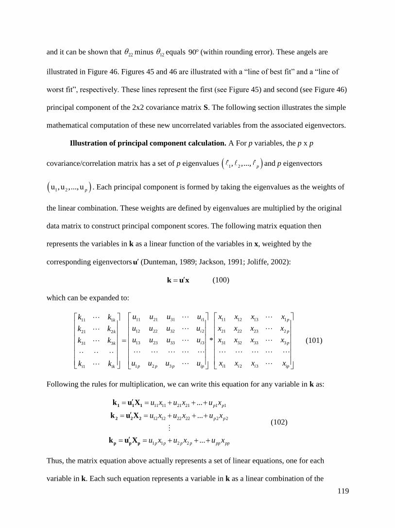
119

and it can be shown that 22 minus 12 equals 90 (within rounding error). These angels are

illustrated in Figure 46. Figures 45 and 46 are illustrated with a “line of best fit” and a “line of

worst fit”, respectively. These lines represent the first (see Figure 45) and second (see Figure 46)

principal component of the 2x2 covariance matrix S. The following section illustrates the simple

mathematical computation of these new uncorrelated variables from the associated eigenvectors.

Illustration of principal component calculation. A For p variables, the p x p

covariance/correlation matrix has a set of p eigenvalues 1 2, ,..., p and p eigenvectors

1 2u ,u ,...,u p . Each principal component is formed by taking the eigenvalues as the weights of

the linear combination. These weights are defined by eigenvalues are multiplied by the original

data matrix to construct principal component scores. The following matrix equation then

represents the variables in k as a linear function of the variables in x, weighted by the

corresponding eigenvectors u (Dunteman, 1989; Jackson, 1991; Joliffe, 2002):

k u x (100)

which can be expanded to:

11 21 31 1 11 12 13 111 1

12 22 32 2 21 22 23 221 2

13 23 33 3 31 32 33 331 3

1 2 31

*

i pk

i pk

i pk

p p p ipi ik

u u u u x x x xk k

u u u u x x x xk k

u u u u x x x xk k

u u u uk k

1 2 3i i i ipx x x x

(101)

Following the rules for multiplication, we can write this equation for any variable in k as:

11 11 21 21 1 1

12 12 22 22 2 2

1 1 2 2

...

...

...

p p

p p

p p p p pp pp

u x u x u x

u x u x u x

u x u x u x

1 1 1

2 2 2

p p p

k u X

k u X

k u X

(102)

Thus, the matrix equation above actually represents a set of linear equations, one for each

variable in k. Each such equation represents a variable in k as a linear combination of the

120

variables in x, multiplied by a weighting coefficient in u. These equations define the principal

component scores, which reflect the variation that each original variable ppx contributes to a

particular principal component pk . The sum of all of the contributions (i.e., weights) of a

particular variable (e.g., x1) for p principal components is equal to 1.0 indicating that all of the

variance in that variable is accounted for by the set of principal components (e.g., Dunteman,

1989). Said differently, each variable contributes a certain amount of variance to the definition of

each principal component. The total variance of a particular principal component is equal to the

eigenvalue associated with the eigenvectors that define that component. So, the new transformed

variables are referred to as principal components while the values that do the transforming are

referred to as the principal component scores (see Figure 47). For a complete guide to working

with principal components in the social and behavioral sciences, see Raykov and Marcoulides

(2008).

Summary of principal component analysis. A Principal Component Analysis (PCA) is

a multivariate data reduction technique and is typically recommended as a precursor to other

multivariate analytic methods. As previously discussed, PCA has a long history with a

complementing geometric and algebraic interpretation. The ability to uncover variance that is

otherwise hidden within a large number of variables is one of the strengths associated with PCA.

Another asset of PCA is the capacity to retain variation from a larger set of correlated variables

in a few new variables that are uncorrelated with each other. These new variables provide a more

parsimonious description of the original data without losing useful variance (Jolliffe, 2002). The

calculations behind PCA are closed form linear transformations that are directly related to

eigenvectors (Jackson, 1991; Jolliffe, 2002) where the variance of each successive component is

maximized. Consequently, PCA is not a form of factor analysis. While it is possible to interpret

principal components, this practice is typically irrelevant in most applications of PCA (see

121

Widaman, 2007). Although the illustrations of PCA computations based on Table 7 were

relatively straightforward (i.e., p = 2 dimensions), more realistic numbers of variables (e.g., p =

40, 60, etc.) are difficult to transform by hand calculations and impossible to plot in p

dimensional space. Still, the basic ideas presented generalize to any number of variables (see

Jackson, 1991).

Method I: Simulation Studies

After discussing the theoretical rational for PCA as a method to extract useful variance

from a large set of variables, and the practical estimation limitations of the inclusive auxiliary

variable strategy, the following discussion more specifically address a method of using principal

component analysis (PCA) to obtain auxiliary variables to better approximate an inclusive

strategy in MI and FIML. The PCA auxiliary variable method (PCAAUX) is assessed using a

series of Monte Carlo simulation studies as well as an in an empirical data example. The purpose

of these simulation studies was to address the following questions: (1) Does the PCA auxiliary

variable (PCAAUX) method converge in a situation where a typical inclusive strategy fails? (2) Is

the inclusion of a smaller set of PCA auxiliary variables (PCAAUX) as beneficial as including all

possible auxiliary variables (AUX; an inclusive strategy)? (3) does this relationship change as a

function of sample size, missing data rate, or the magnitude of variable correlations? (4) does a

non-linear MAR mechanism influence the performance of PCAAUX relative to AUX? and (5)

what is the relative performance of PCAAUX and AUX in an empirical data example?

Design and Procedure

Convergence. As previously noted, research suggests that MI and FIML tend to

experience convergence problems in situations with a complex missing data pattern and

insufficient coverage for a particular parameter estimate (Enders, 2010; Graham, Cumsille, &

Shevock, in press; Graham, 2009; Savalei & Bentler, 2009). Although these discussions are

useful to highlight a known limitation in the field, they may not offer compelling evidence

122

regarding the practical performance of MI and FIML estimation routines across various software

packages. In the following section, a small simulation study was used to demonstrate

convergence issues in both MI and FIML even when reasonable resolutions are pursued across

selected statistical software packages. In order to demonstrate the potential for PCA auxiliary

variables (PCAAUX) to convergence in a situation where a large number of typical auxiliary

variables (AUX) fail, these simulations were repeated using the PCAAUX variables.

Population Model. To demonstrate a situation where modern methods fail to converge,

consider a research scenario where it is of interest to estimate the mean vector and covariance

matrix between two variables, X and Y. Additionally, suppose an inclusive strategy where 48

additional auxiliary variables (AUX1 – AUX48) are included. Let the associations across all

variables be set to ρ = .30 and the means and variances set at µ = 0.0 and σ2 = 1.0.

Data Generation. Mplus 6.0 (Muthén & Muthén, 1998–2010) was used to generate the

population model outlined previously using one multivariate normal data set of size N = 1,000.

After data generation, each dataset was saved to a file and then imported into SAS 9.3 (SAS

Institute Inc., 2011) for sample size selection and missing data generation. In line with

Asparouhov and Muthén (2010), three different sample sizes including N = 50, N = 100, and N =

500 were considered. These values were intended to represent a practical set of possible sample

sizes. In order to obtain a particular sample size, the SURVEYSELECT procedure in SAS was

used to draw a random sample from the largest sample size investigated (i.e., N = 1,000). This

method was used to minimize the influence of sampling variability in the simulated results. After

sample size selection, SAS was used to impose MAR missing data rate of 30% on all variables

except X. The MAR mechanism was generated by deleting values based on the lower distribution

of X, which resulted in a general missing data pattern. Figure 47 presents a graphical depiction of

the missing data pattern. While these simulation conditions were not intended to be

comprehensive, it was of interest to provide a practical demonstration of convergence failure

123

given a representative missing data rate (e.g., 30%) and pattern (e.g., general pattern) for a

moderate to large number of variables (e.g., p = 50).

After generating the data and implementing the specified missing data rate, the data were

read into a selected set of popular software programs including: (a) SAS 9.3, (b) Mplus 6.12, and

(c) SPSS 20. For this demonstration three sequential imputation methods were used including (1)

the first method was based on default settings in each program, (2) the next method increased the

iterations to 10,000, (3) the following methods either added a ridge prior equal to 10 (in SAS) or

increased the MCMC iterations (Mplus). Similarly, three sequential likelihood-based methods

were used including: (1) default settings, (2) increasing the iterations to 10,000, and (3) lowering

the convergence criteria to .01. These conditions were based on recommendations in the

literature (see Enders, 2010; Graham, 2009; Savalei & Bentler, 2009; Schafer, 1997). For

example, Schafer (1997) suggested that a ridge prior be used when, “…either the data are sparse,

or because such strong relationships exist among the variables that certain linear combinations of

the columns of Y exhibit little or no variability,” (p. 155-156). The three sequential imputation

approaches and the likelihood-based approaches were intended to show that convergence failure

may occur even when reasonable steps are taken to generate a solution.

Analysis Models. While MI was employed in all three programs, FIML was only

available in Mplus. Therefore, MI represents the only method that was assessed across each of

the selected software packages. Importantly, this data example was not intended to compare the

various software packages as they utilize differing algorithms for MI. Rather, the goal was to

generate data that produced estimation problems to highlight the idea that MI and FIML may fail

to converge on an acceptable solution. For each condition, the missing data model incorporated

X, Y and all auxiliary variables (p = 48). In order to complicate the model, two additional

interaction terms were generated representing variables with non-linear variation that add

complexity by infusing high collinearity into the estimation process. The first interaction term

124

was created by multiplying the first and the second auxiliary variables together (i.e., AUX12)

while the second interaction term was generated by multiplying the third and the fourth auxiliary

variables together (i.e., AUX34). These new variables were included among the original 48

auxiliary variables in the missing data model (i.e., 50 total auxiliary variables) and along with the

two analysis variables (i.e., X and Y).

As previously mentioned, statistical theory and simulation based research supports an

“inclusive strategy” where as many auxiliary variables are included as possible (e.g., Collins,

Schafer, & Kam, 2001; Enders, 2010). However, the complexity of the missing data handling

procedure typically increases with the addition of each additional auxiliary variable, especially

when the auxiliary variables have missing data. Practically, there is a limit to the number of

auxiliary variables that can be incorporated before the missing data handling routine (e.g., FIML,

MI) will fail to converge on a solution (e.g., Enders, 2010; Graham, Cumsille, & Shevock, in

press). The determination of this limit may relate to many dataset specific factors and is likely to

vary across a specific set of variables. For instance, the amount of missing information, the

number of variables in the model (i.e., complexity of the model) and the presence of high

collinearity have been shown to influence the convergence of FIML and MI and may lead to

estimation failure (e.g., Enders, 2010). Large data sets can present an obvious challenge, as it is

possible to have hundreds of potential auxiliary variables with various rates of missing data and a

greater potential for multicollinearity problems. Therefore, the goal of this small simulation was

simply to demonstrate that the PCAAUX method converges in situations where a typical inclusive

strategy fails to converge. An investigation into the quality of a PCAAUX relative to a typical

inclusive strategy (AUX) is presented next.

Outcomes. In addition to assessing convergence based on software error messages and

graphical displays (discussed previously), the mean squared error, a measure of the quality of

missing data recovery, was calculated based on the formula (see Asparouhov & Muthén, 2010):

125

2

1

1( )

p

j j

j

MSEp

(103)

where p is the number of variables, j represents the true population value and j is the average

mean over Yj imputed data sets. In the case of FIML, j represents the true population value as

before and j is the estimated variable mean for the jth

variable.

Relative Performance. The relative performance of AUX and PCAAUX was examined

across seven independent variables (magnitude of correlations, homogeneity of correlations

across auxiliary variables, rate of missing, missing data mechanism, missing data patterns,

number of auxiliary variables, and sample size) on four dependent variables (raw parameter

estimate bias, percent bias, standardizes bias, & relative efficiency). The manipulated

independent variables represent factors known to influence the performance of auxiliary

variables.

For example, the effectiveness of auxiliary variables is expected to improve as the

magnitude of correlations increase given a particular rate of missing and sample size (Collins,

Schafer, & Kam, 2001). As Enders (2010) noted, “…omitting a correlate of missingness was not

that detrimental when the correlation was weak (e.g., r ≤ .30), but the estimates became

increasingly biased as the correlation between the auxiliary variable and the incomplete analysis

variable increased in magnitude,” (p. 129). This relationship explains the suggestion provided by

many methodologists (e.g., Collins, et al., 2001) to locate auxiliary variables that exceed an

association of about r = .40 with the variables with missing data. This idea is so prevalent in the

literature that it is not uncommon for methodologists to define auxiliary variables as,

“…variables that are highly correlated with the analysis model variables, but not necessarily part

of the one’s analysis model,” (Graham, Cumsille, & Shevock, 2013, p. 13).

Additionally, numerous Monte Carlo simulation studies on the topic of missing data

assess the influence of sample size and rate of missing data on parameter bias, relative

126

efficiency, and convergence failure (e.g., Bodner, 2008; Enders & Bandalos, 2001; Enders &

Peugh, 2004; Graham, Olchowski, & Gilreath, 2007; Wothke & Arbuckle, 1996; Yuan, 2009).

For instance, Collins, Schafer and Kam (2001) noted that when the MAR assumption is violated

the resulting estimation may not be substantially biased unless the rate of missing data is high.

Bias has been shown to increase with the missing data rate (Enders & Bandalos, 2001).

Some research suggests that sample size may have little effect on relative efficiency and

bias (Enders & Bandalos, 2001); though bias expressed relative to the standard error may be

more sensitive (Enders, 2003). Further, small sample sizes are also associated with lower

statistical power which may make bias difficult to detect even when the rate of missing is

relatively high (Yuan, 2009). Research also notes that small sample sizes may increase

estimation failure (Enders & Bandalos, 2001; Yoo, 2009) especially with high missing data rates

(Newman, 2003).

The choice to examine two missing data mechanisms was influenced by Collins, Schafer,

and Kam (2001), who noted that non-linear causes of missingness may generate bias even with a

missing data rate less than 25%. They also discussed the potential to minimize this bias by

including the non-linear information in the missing data handling procedure. Auxiliary variables

that include variance from a non-linear MAR process are expected to improve estimation across

various sample size and missing data rates.

For instance, the performance of both PCAAUX and AUX are expected to be similar as

PCAAUX should contain the important information from AUX. That is, the bias associated with

AUX should be similar to the bias observed with PCAAUX even though the latter contains far

fewer variables (e.g., 1 PCAAUX vs. 8 AUX). This relative relationship should improve in parallel

as the magnitude of correlations (among the auxiliary variables and the variable with missing

data) increase, and with sample size increases given a particular rate of missing and number of

auxiliary variables. Both techniques are expected to outperform the absence of any auxiliary

127

variables. Additionally, PCAAUX is expected to improve parameter estimation beyond the

improvement of AUX given a non-linear MAR type of missingness. This situation mimics a

scenario where the cause of missingness is an unknown non-linear process that is only captured

via the all-inclusive PCAAUX approach.

In order to specify the reasonable values for each condition, Monte Carlo simulation

studies published in the social sciences on the topic of missing data handling between 1996 and

2011 were reviewed (see Table 8 for a summary). Based on this literature review, the following

levels were selected: (a) magnitude of correlations (ρ = 0 to .80), (b) homogeneity of correlations

across auxiliary variables (uniform, moderate homogeneity, low homogeneity), (c) rate of

missing (10% to 80%), (d) missing data mechanism (MAR, non-linear MAR), (e) missing data

patterns (monotone, and general), (f) number of auxiliary variables (0 to 8), and (g) sample size

(N = 50 to 1000). These levels represent a wide range of conditions found in the reviewed

literature and were selected to provide a useful context in which to assess the relative

performance of PCAAUX and AUX.

Population Model. For the first study, a bivariate normal correlation model between the

variables X and Y were used to generate population data for the associated simulation studies.

Figure 48 illustrates this population model including the 8 additional auxiliary variables that

were also incorporated. This data generation model was an expanded version of the model used

by Collins, Schafer, and Kam (2001) and Enders (2010). As Demonstrated in Figure 48, within a

given cell design, the population correlation between X and Y was fixed at ρ = .30 as was the

relationship between the auxiliary variables and X. To manipulate the homogeneity of

associations among the auxiliary variables, three correlation patterns were introduced. The

population model for the uniform condition had identical correlations of ρ = .30 for all eight

auxiliary variables. In the moderate condition, one fourth of the correlations were set at ρ = .20;

another fourth was set at ρ = .25; a third fourth was set at ρ = .35; and the last fourth was set to ρ

128

= .40. In the low homogeneity condition one fourth of the correlations were set at ρ = .10;

another fourth was set at ρ = .20; a third fourth was set at ρ = .40; and the last fourth was set to ρ

= .50. The moderate and low homogeneity conditions generated model-implied correlations that

varied in magnitude among each fourth of the specified correlations. Regardless of the auxiliary

variable magnitude, the average association between the auxiliary variables and Y was about ρ =

.30 which is considered a conservative lower bound for exerting influence on the imputation

model (see Collins, Schafer, & Kam, 2001; Graham, 2009). As illustrated in Figure 48, the

magnitude of correlations ranged from ρ = 0 to .80 rather than from ρ = 0 to 1.0 based on the

limitations of Equation 20. That is, because some associations were set to ρ = .30 the range of

other relationships were constrained so that the population variance and covariance matrix was

positive definite.

Data Generation. Data generation involved two separate sets of simulation studies

including simulations using FIML and simulations using MI. In the following discussion, each

approach will be discussed in turn. For the first study, Mplus 6.0 (Muthén & Muthén, 1998–

2010) was used to generate ten variables: X, Y, and eight auxiliary variables in 1,000 multivariate

normal data sets of size 1,000 for each set of population values using the MONTECARLO

command. These simulation studies were external Monte Carlo simulations (i.e., the data are not

generated and analyzed in one step within Mplus (see Muthén & Muthén, 2010). Rather the

simulated data from all replications were saved to a file. This was done primarily for two

reasons: (1) The Mplus statistical program has a built in tool that generates missing values from a

logistic regression model which methodologists note is difficult to accurately control (see

Enders, 2009; Muthén & Muthén, 2010); therefore, the SAS 9.3 statistical program was chosen

to implement missing data and (2) Mplus does not currently support principal component

analysis, which was relevant to the current study.

129

To obtain a particular sample size, the SURVEYSELECT procedure in SAS 9.3 (SAS

Institute Inc., 2011) was used to draw a random sample from the largest sample size investigated

(i.e., N = 1,000). This method was used to minimize the influence of sampling variability in the

simulated results. After data generation and sample size selection, SAS 9.3 was used to generate

principal component scores using the PROC PRINCOMP procedure. Note that the variance used

to generate the principal components did not include the variables X and Y as this would not

provide a low bound for the effectiveness of the imputation model. That is, it could be argued

that the relative performance of PCAAUX is driven by the inclusion of variance from X and Y.

Then, SAS was used to impose one of the proposed missing data mechanisms (MCAR,

MAR, non-linear-MAR; Little & Rubin, 2002) on Y with one of two missing data patterns. The

first pattern was a monotone missing data pattern (i.e., where missingness occurs for some of the

values of Y; Enders, 2010; Little & Rubin, 2002) and the second pattern was a general missing

data pattern (i.e., with missingness scattered throughout the data in a seemingly random fashion;

see Figure 49). There are numerous research situations that lead to the monotone pattern of

missing data and it has been widely used in the literature to study missing data (e.g., Little and

Rubin, 1987; Enders, 2010). For example, let Y represent a questionnaire item with missing data

and let X represent a demographic variable, like age, with no missing values. The variable X

could also represent a fixed variable controlled by the experimenter or any other variable with

complete data. While a monotone pattern is of primary interest for the majority of the current

simulation studies, the general missing data pattern will provide useful information regarding

convergence rates for various observed data coverage rates and presents a more appropriate

missing data situation (Enders, 2010).

For each missing data mechanism, missing data were imposed by generating a random

variable and then distributing it through FORMAT statement using SAS 9.3. This procedure

allows for the specification of a particular missing data pattern and the random audition of values

130

of selected variables (e.g., Y) for deletion in order to obtain a particular missing data percentage.

To select a variable (or set of variables) for deletion, another DATA statement was used to

generate an array that referenced the variable of interest. Then, a uniform random number vector

was used to pair the probability of missing data with the specified missing data pattern.

Under the MCAR mechanism, a data point was subsequently deleted if the corresponding

uniform random number auditioned a value from the “misspattern” FORMAT statement that

related to the specified missing data rate. In this way the probability that Y, for instance, contains

missingness can be written as: p(Ymis | data) = p(Ymis) where the propensity for missingness is

unrelated to any measured or unmeasured variables (a random process). A key point of this study

was to assess the power of PCAAUX relative to all possible typical auxiliary variables (AUX;

Aux1 – Aux8). MCAR missingness is unbiased and is useful to assess statistical power associated

with the inclusion of an auxiliary variable (or set of auxiliary variables) relative to a model where

auxiliary variables are omitted. That is, including auxiliary variables (PCAAUX or AUX) into a

MCAR situation will not impact parameter estimate bias but should influence statistical power.

Another main point of this study was to assess the relative performance of PCAAUX and

AUX across a set of conditions. Therefore, another set of simulations required a MAR missing

data mechanism. The MAR mechanism required a slightly different step than the MCAR

mechanism previously described. Specifically, the deciles of a selected variable (e.g., the first

auxiliary variable; Aux1) were found using the SAS UNIVARIATE procedure. These deciles

were then be used to divide the distribution of Aux1 into 10 equal portions. This was done so that

the kth

decile for Aux1 is a value (e.g., p) such that the probability that Aux1 will be less than p is

at most k / p and the probability that Aux1 will be more than p is at most (p - k ) / p. Thus, a data

point was deleted if Aux1 was less than or equal to a particular decile. In this manner the

probability that Y contains missingness can be written asmis mis 1 qu( | Data) ( | , )

iP Y P Y q . That is,

the probability of missingness (Ymis) is related to the ith

decile of Aux1. Among other things, this

131

procedure mimics a scenario in which missing values on a variable (i.e., Y) result from low

scores on another variable in the data set. This MAR process is similar to that modeled by

Muthén et al. (1987) and Enders and Bandalos (2001).

Also of interest in the current study was the influence of a non-linear MAR mechanism

on the performance of PCAAUX relative to AUX. This scenario required further simulations

where missingness was produced in a similar manner to that described previously for the MAR

condition. However, this time rather than utilizing the decile of a particular auxiliary variable

(e.g., Aux1), the decile of an interaction term was used (e.g., Aux1*Aux2). A data point was

deleted if Aux1*Aux2 was greater than or equal to a particular decile.

For the MI approach, the simsem package in the R program (Pornprasertmanit, Miller, &

Schoemann, 2012) was used to generate ten variables: X, Y, and eight auxiliary variables in 1,000

multivariate normal data sets of size 1,000 for each set of population values, as was specified for

the FIML condition. The MI method utilized the same simulation designs (i.e., missing data

mechanism, principal components analysis, etc.) were carried out within the R program.

Analysis Models. The analytic model for these simulations is the association between Y

and X. The variables Aux1 – Aux8 were used as auxiliary variables. For the FIML approach, after

generating the principal component scores, the data from all replications were saved to a file.

Then, Mplus 6.0 was used to analyze the data for each sample replicate. Auxiliary variables were

incorporated into the FIML estimation routine via the AUXILIARY (m) option (via the saturate

correlates model; see Graham, 2003; Asparouhov & Muthén, 2008). Then, the results of each

simulation (i.e., parameter estimates and standard errors) were saved to a data file and collected

using a series of SAS macros. For the MI approach, the simsem package in R was used to

analyze the data for each sample replicate. Auxiliary variables were incorporated into the MI

estimation routine using AMELIA with 20 imputations (Honaker, King, & Blackwell, 2011).

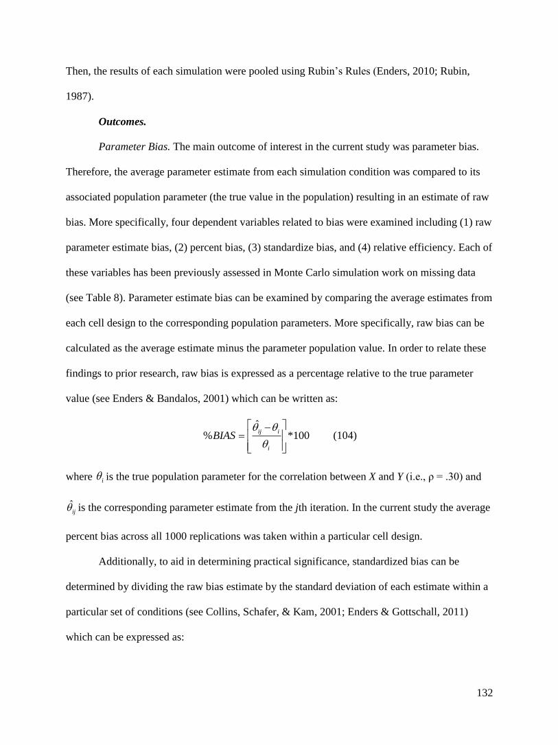
132

Then, the results of each simulation were pooled using Rubin’s Rules (Enders, 2010; Rubin,

1987).

Outcomes.

Parameter Bias. The main outcome of interest in the current study was parameter bias.

Therefore, the average parameter estimate from each simulation condition was compared to its

associated population parameter (the true value in the population) resulting in an estimate of raw

bias. More specifically, four dependent variables related to bias were examined including (1) raw

parameter estimate bias, (2) percent bias, (3) standardize bias, and (4) relative efficiency. Each of

these variables has been previously assessed in Monte Carlo simulation work on missing data

(see Table 8). Parameter estimate bias can be examined by comparing the average estimates from

each cell design to the corresponding population parameters. More specifically, raw bias can be

calculated as the average estimate minus the parameter population value. In order to relate these

findings to prior research, raw bias is expressed as a percentage relative to the true parameter

value (see Enders & Bandalos, 2001) which can be written as:

ˆ% *100

ij i

i

BIAS

(104)

where i is the true population parameter for the correlation between X and Y (i.e., ρ = .30) and

ˆij is the corresponding parameter estimate from the jth iteration. In the current study the average

percent bias across all 1000 replications was taken within a particular cell design.

Additionally, to aid in determining practical significance, standardized bias can be

determined by dividing the raw bias estimate by the standard deviation of each estimate within a

particular set of conditions (see Collins, Schafer, & Kam, 2001; Enders & Gottschall, 2011)

which can be expressed as:

133

ˆStandardized 100*

ij i

ij

BIASSE

(105)

where ijSE is the standard error from the thj iteration. Collins, Schafer and Kam (2001) report

that standardized bias estimates that exceeds 40% - 50%, “begin to have noticeable adverse

impacts on efficiency, convergence, and error rates,” (p. 340). They suggest a standardized bias

absolute value greater than 40% as practically significant.

Relative Efficiency. Another prevalent standard metric reported below is the Root-mean-

squared error (RMSE), the average squared difference between the estimate ˆij and the

population value i (Collins, Schafer, & Kam, 2001; Enders, 2003; MacDonald, Thurston &

Nelson, 2000; Roth, Switzer & Switzer, 1999; Zhang & Walker, 2008). This metric combines

efficiency and bias information and is typically reported in relation to accuracy (Collins, Schafer,

& Kam, 2001). A purer measure of efficiency is given by the ratio of sampling variances for the

parameter of interest (i.e., rxy) called relative efficiency (RE; Arbuckle, 1996; Enders &

Bandalos, 2001; Wothke, 2000) which can be illustrated by:

2

2

i

PCA

qRE

AUX

(106)

where 2

iq is the sampling variance of the parameter of interest (rxy) from the ith auxiliary

variable and 2

PCAAUX is the corresponding sampling variance of the principal component

auxiliary variable method. The average standard error estimates under each condition can be

compared to the true standard error (i.e., based on the Monte Carlo simulation standard deviation

across replications) in a similar fashion as the parameter bias to determine the degree of over or

under estimation (see Newman, 2003).

Method II: Empirical Study

134

In addition to the simulation work, we investigated the relative performance of typical

auxiliary variables (AUX) and a smaller set of PCA auxiliary variables (PCAAUX) in an empirical

data example. Using actual data we investigated three conditions: (a) no auxiliary variables were

employed, (b) all possible AUX were used, and (c) the PCAAUX approach was used. This

example uses data from a previously reported sample assessing the Early Communication

Indicator (ECI), a measure for intervention decision-making in infants and toddlers (see

Greenwood & Walker, 2010). Participants were infants and toddlers recruited from Early Head

Start (EHS) programs and included children between the ages of 8 and 37 months and the

percent missing was 57%.

Procedure and variables

Researchers collected key communicative behaviors including: gestures, vocalizations,

single words, and multiple words in 1-month intervals representing 33 separate occasions

between the ages of 5 to 37 months (see Greenwood & Walker, 2010 for details). The data were

then transformed to reflect mean estimates separated by three months which generated 11

measurement occasions between ages of 5 to 37 months. For the current example, the first

measurement occasion (including months 5, 6 and 7) for each key skill variable was not used

because single and multiple word usage was not observed during this developmental period

resulting in 40 key skill variables (10 measurement occasions x 4 variables; see Table 9). Raw

data plots are shown in Figure 55.

Empirical missing data. All 40 variables had at least one missing value on a case, 569 of

the 570 cases had at least one missing value on a variable, and that 13,003 of the 22,800 values

(cases × variables) are missing; therefore, 57% of the data were missing. There were 308 missing

data patterns dispersed throughout the data in a seemingly random fashion (see Enders, 2010);

however, as demonstrated in Table 9, much of the missing data occurred at the 10th

measurement

occasion (i.e., 35 – 37 months).

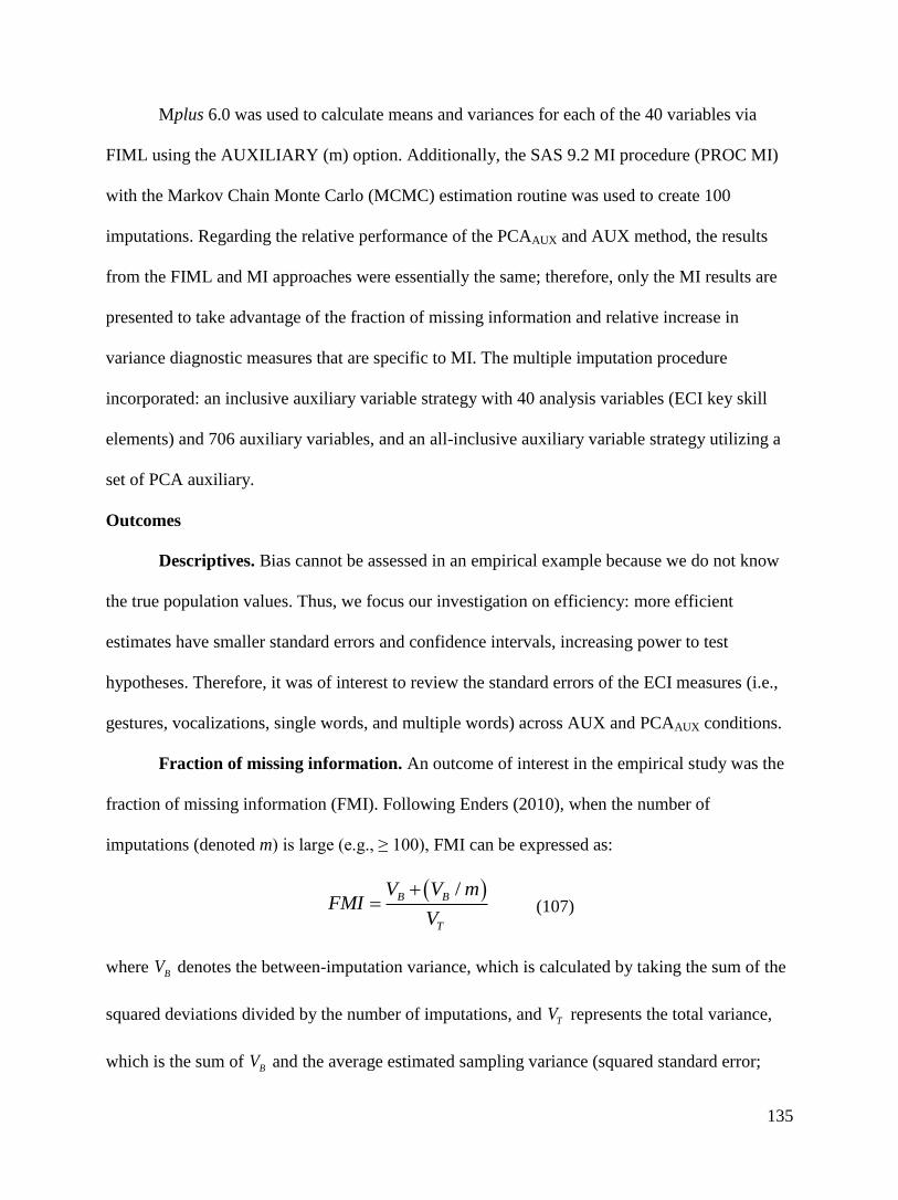
135

Mplus 6.0 was used to calculate means and variances for each of the 40 variables via

FIML using the AUXILIARY (m) option. Additionally, the SAS 9.2 MI procedure (PROC MI)

with the Markov Chain Monte Carlo (MCMC) estimation routine was used to create 100

imputations. Regarding the relative performance of the PCAAUX and AUX method, the results

from the FIML and MI approaches were essentially the same; therefore, only the MI results are

presented to take advantage of the fraction of missing information and relative increase in

variance diagnostic measures that are specific to MI. The multiple imputation procedure

incorporated: an inclusive auxiliary variable strategy with 40 analysis variables (ECI key skill

elements) and 706 auxiliary variables, and an all-inclusive auxiliary variable strategy utilizing a

set of PCA auxiliary.

Outcomes

Descriptives. Bias cannot be assessed in an empirical example because we do not know

the true population values. Thus, we focus our investigation on efficiency: more efficient

estimates have smaller standard errors and confidence intervals, increasing power to test

hypotheses. Therefore, it was of interest to review the standard errors of the ECI measures (i.e.,

gestures, vocalizations, single words, and multiple words) across AUX and PCAAUX conditions.

Fraction of missing information. An outcome of interest in the empirical study was the

fraction of missing information (FMI). Following Enders (2010), when the number of

imputations (denoted m) is large (e.g., ≥ 100), FMI can be expressed as:

/B B

T

V V mFMI

V

(107)

where BV denotes the between-imputation variance, which is calculated by taking the sum of the

squared deviations divided by the number of imputations, and TV represents the total variance,

which is the sum of BV and the average estimated sampling variance (squared standard error;

136

Enders, 2010) across m imputations. FMI reflects the relationship between the missing data

pattern and the magnitude of associations among variables where highly related variables with

good coverage produce the lowest FMI value. That is, missing data does not greatly influence the

sampling variance. Conversely, weakly related variables with poor coverage generate a high

FMI. In this situation the missing data may significantly inflate the sampling variance. The

interpretation of FMI is straightforward. For instance, when FMI = .004 less than 1% (e.g.,

0.4%) of the sample variance is related to missing data.

Relative increase in variance. Another important outcome was the relative increase in

variance (RIV). While the FMI provides the percentage of sample variance related to missing

data, the RIV yields a measure of the relative increase in variance (between-imputation variance

relative to within-imputation variance) such that RIV = 0 indicates that the variance was not

influenced by missing data. Conversely, RIV = 1 suggests that the between-imputation variance

is equivalent to the within-imputation variance (see Enders, 2010). As illustrated by Enders, RIV

can be written as:

/

1

B B

W

V V m FMIRIV

V FMI

(108)

where BV , TV , and m are defined as previously indicated while WV is the sampling error that

would have resulted given no missing data.

Simulation Results

For ease of presentation, a select set of conditions are presented to highlight the relative

performance of AUX and PCAAUX in relation to parameter estimate bias.

Convergence

AUX strategy. FIML in Mplus was assessed for each sample size by sequentially

implementing methods 1 – 3 (as previously described) until convergence was reached. Given the

smallest sample size N = 50 none of the likelihood-based models (i.e., 1 – 3 defined above)

137

converged. Note that this model was not identified, as there were more variables than cases.

Further, this model had less information to inform the likelihood-based estimation than models

with more cases. That is, 30% missing data from N = 50 provides less coverage than 30%

missing from N = 100 or N = 500. These points are reflected in the error code generated by

Mplus that noted,

“THE MISSING DATA EM ALGORITHM FOR THE H1 MODEL HAS NOT CONVERGED

WITH RESPECT TO THE PARAMETER ESTIMATES. THIS MAY BE DUE TO SPARSE DATA

LEADING TO A SINGULAR COVARIANCE MATRIX ESTIMATE. INCREASE THE NUMBER

OF H1 ITERATIONS. NOTE THAT THE NUMBER OF H1 PARAMETERS (MEANS,

VARIANCES, AND COVARIANCES) IS GREATER THAN THE NUMBER OF OBSERVATIONS.

NO CONVERGENCE. SERIOUS PROBLEMS IN ITERATIONS.”

With a sample size of N = 100, FIML failed to converge using the default settings and an

error message noted no convergence and the presence of a singular covariance matrix. However,

FIML was able to converge when the number of iterations were increased resulting in MSE =

0.4221. Further, given the largest sample size N = 500 the default settings converged with MSE

= 0.3981. While this demonstration of convergence failure is not intended to be inclusive, it does

indicate that failure may occur with only 30% missing data given a large enough set of auxiliary

variables. As shown above a larger sample size was associated with a lower number of iterations

needed to reach convergence. Additionally, the model conditions including N = 500 and the

default estimation model provided a lower MSE estimate indicating a more accurate imputation

procedure than the conditions including N = 100 and the estimation model with increased

iterations.

MI within the SAS statistical program was assessed for each sample size by sequentially

implementing methods 1 – 3 (as described above) until convergence was reached. As with the

FIML method, the smallest sample size N = 50 did not converge across any of the imputation

138

models. The error code generated by SAS included, “WARNING: The EM algorithm (MLE)

fails to converge after 200 iterations. You can increase the number of iterations (MAXITER=

option) or increase the value of the convergence criterion (CONVERGE= option). WARNING:

The EM algorithm (posterior mode) fails to converge after 200 iterations. You can increase the

number of iterations (MAXITER= option) or increase the value of the convergence criterion

(CONVERGE= option). WARNING: The initial covariance matrix for MCMC is singular. You

can use a PRIOR = option to stabilize the inference. WARNING: the posterior covariance matrix

is singular. Imputed values for some variables may be fixed.” While the sample size of N = 100

demonstrated convergence failure under the default settings, and marked instability under

increased iterations, convergence was reached via a prior ridge which resulted in MSE = 0.4326.

The largest sample size N = 500 also revealed marked instability until a prior ridge was added

resulting in MSE = 0.4009. Given that the N = 100 and the N = 500 sample sizes both needed a

prior ridge to successfully converge, the larger sample size provided a lower MSE estimate

indicating a more accurate imputation procedure (see Asparouhov & Muthén, 2010).

Additionally, the convergence speed of the imputation model based on N = 500 was much faster

than the imputation model based on N = 100. Specifically, the sample size of N = 500 converged

within 116 MCMC iterations while the sample size of N = 100 resulted in convergence within

342 MCMC iterations.

MI within the Mplus statistical program was assessed for each sample size by

sequentially implementing methods 1 – 3 (as described above) until convergence was reached.

As with the prior models, none of the imputation models properly converged with the smallest

sample size of N = 50. Mplus generated the following error code,

“PROBLEM OCCURRED DURING THE DATA IMPUTATION. YOU MAY BE ABLE TO

RESOLVE THIS PROBLEM BY SPECIFYING THE USEVARIABLES OPTION TO REDUCE

139

THE NUMBER OF VARIABLES USED IN THE IMPUTATION MODEL. SPECIFYING A

DIFFERENT IMPUTATION MODEL MAY ALSO RESOLVE THE PROBLEM.”

Given the sample size of N = 100 MI in Mplus converged after increasing the MCMC iterations

to 10,000 resulting in a MSE = 0.4228. Moreover, the sample size of N = 500 converged by

increasing the iterations where the MSE = 0.3983.

MI within the SPSS statistical program was assessed sequentially as previously discussed

in relation to the SAS program. However, none of the SPSS imputation models (e.g., Imputation

Model 1 – 3) converged for any of the specified sample sizes. The error message generated by

SPSS for each condition simply stated, “Not Imputed (Too Many Missing Values)”.

PCAAUX Strategy. Regarding the PCAAUX method, principal component scores were

generated from the p = 50 auxiliary variables, which resulted in 10 PCA variables that accounted

for approximately 80% of the variance in the auxiliary variables. Each of the FIML and MI

models were run where 10 PCAAUX variables were used in place of the 50 AUX variables. The

purpose of this approach was to determine whether the PCAAUX method converged in conditions

where a typical inclusive auxiliary variable strategy failed.

FIML in Mplus was assessed as before for each sample sizes by sequentially

implementing methods 1 – 3 (i.e., default settings, increased iterations, decreased convergence

criteria) until convergence was reached. Given the smallest sample size of N = 50 the default

model converged under the PCAAUX approach resulting in MSE = 0.0240. Note that this model

was identified due to the use of PCAAUX variables, as there were more cases (i.e., 50) than

variables (i.e., 12). With a sample size of N = 100, FIML was able to converge under the default

settings resulting in MSE = .0225. Further, given the largest sample size N = 500 the default

settings converged with MSE = .0125. While this demonstration is not comprehensive, it does

suggest that to the use of PCAAUX variables (a smaller uncorrelated subset of the original

140

variables) converged faster and related to a much smaller MSE estimate than incorporating all

possible auxiliary variables.

MI within the SAS statistical program was assessed for each sample size by sequentially

implementing methods 1 – 3 (i.e., default settings, increase iterations, utilize a prior ridge) until

convergence was reached. As with the FIML method, the smallest sample size N = 50 converged

within 31 MCMC iterations using the default settings which resulted in MSE = .0387. Further,

the sample size N = 100 converged within 27 MCMC iterations using the default settings which

resulted in MSE = .0350. The sample size N = 500 converged within 25 MCMC iterations using

the default settings which resulted in MSE = .0182. As demonstrated, the convergence speed of

the PCAAUX models was fast and increased with sample size. Additionally, larger sample sizes

provided a lower MSE estimate signifying more accuracy in the imputation process (Asparouhov

& Muthén, 2010).

MI within Mplus was assessed for each sample size by sequentially implementing

methods 1 – 3 (as described previously) until convergence was reached. As with the prior

models, smallest sample size of N = 50 converged with MSE = .0243. Given the sample size of N

= 100 MI in Mplus converged with MSE = .0159. Moreover, the sample size of N = 500

converged where the MSE = .0112.

MI within the SPSS statistical program was assessed size by sequentially implementing

methods 1 – 3 (as described previously) until convergence was reached. The N = 50 sample size

converged under the default settings with MSE = .0394. Similarly, the N = 100 sample size

converged under the default settings with MSE = .0239 and the largest sample size N = 500

converged using the default settings resulting in MSE = .0133. The quality of the information

retained in the PCAAUX approach is addressed next.

Linear MAR performance

A key point of this study was to determine if the inclusion of a PCA auxiliary variable

141

(PCAAUX) is as beneficial as an inclusive strategy using typical auxiliary variables (AUX), given

that the PCAAUX approach represents a reduced set of variables that are less likely to cause

convergence failure. The following discussion highlights results from the condition with a 60%

MAR missing data rate and a monotone missing data pattern where the population correlation

between the auxiliary variables (Aux1 – Aux8) and Y was fixed at ρ = .60 in the population

model. The presented relationships hold across sample size and missing data rates though large

sample sizes decrease the observed bias (illustrated in Table 10) and larger missing percentages

result in more bias.

Further, regarding the relative performance of the PCAAUX and AUX method, the results

from the FIML and MI studies were essentially the same; therefore, only the FIML results are

presented. Also, while the correlation magnitude between the auxiliary variables and the variable

with missingness influenced parameter estimates, this study found no differences in the

homogeneity of auxiliary variable correlations. Consequently, the subsequent presentation is

limited the uniform model.

Table 10 contains results showing the impact of PCAAUX and AUX on parameter

estimation raw bias, standardized bias, and percent bias across various sample sizes. The AUX

and the PCAAUX approach demonstrate essentially no bias across various sample sizes, though

the PCAAUX method performs slightly better with smaller sample size relative to the AUX

method. For instance, the AUX method that included all possible auxiliary variables (Aux1 –

Aux8) produced a slight bias of 1% or less with more bias associated with lower sample sizes. In

comparison, the PCAAUX approach that utilized a single auxiliary variable (which accounted for

approximately 80% of variance among the 8 simulated auxiliary variables) produced a bias of

0.16% or less with more bias associated with lower sample sizes.

Also of interest is the “no auxiliary variable” condition which is used as a point of

comparison between PCAAUX and AUX beyond relative contrasts. The most notable bias is

142

found when no auxiliary variables are used and the sample size was small (see Table 10). This

result is not surprising because excluding correlates of missingness conclusively shows

parameter estimate bias and is not in line with current missing data theory regarding the use of

auxiliary variables (see Collins et al., 2001; Enders, 2010). Said differently, when the auxiliary

variables are not included the MAR mechanism effectively becomes a MNAR mechanism and

the parameter bias is maximized for each condition.

Non-linear MAR performance

Another goal of this study was to assess the relative performance of PCAAUX and AUX

when the cause of missingness is nonlinear. As illustrated in Table 11, the AUX method that did

not include the AUX1*AUX2 interaction term (i.e., the cause of missingness) produced a

standardized bias of up to .10 (i.e., 1/10 of a standard error) with an associated 22% bias. In

comparison, the PCAAUX approach utilized a single principal component auxiliary variable that

included the nonlinear information from the AUX1*AUX2 interaction term produced a

standardized bias of no more than .005 with the largest percent bias reaching 1.7%. As seen in

Table 11, the magnitude of bias across both methods decreased with sample size.

Table 12 presents the relative performance of PCAAUX and AUX where the AUX variable

list incorporated the additional non-linear cause of missingness (i.e., AUX1*AUX2). This

condition is perhaps a more reasonable comparison among AUX and PCAAUX because both

procedures reflect the MAR mechanism. The addition of the interaction term decreased bias. For

example, the sample size of N = 200 in Table 11 included an 73.5% bias when no auxiliary

variables were included, an 8% bias when all possible auxiliary variables were included

excluding the interaction term, and less than 1% bias when all possible auxiliary variables

including the interaction term was included or when the one PCA auxiliary variable was

included. This finding was consistent across sample sizes except under small sample size

conditions where the PCAAUX approach shows less bias than the AUX approach with the

143

interaction term.

Relative efficiency. Following Enders and Bandalos (2001), relative sampling variance

was used to determine the relative efficiency (RE) of parameter estimates based on the PCAAUX

relative to the AUX method where RE indicates the sample size increase need by the AUX

method to reach the same efficiency as the PCAAUX method (e.g., RE = AUX / PCAAUX; see

Table 13). For instance, a RE estimate of 1.100 indicates that the sample size for the AUX (i.e.,

AUX1 – AUX8) would need to increase by 10% to have the same efficiency as PCAAUX.

While the sampling variability was smaller with larger sample sizes, RE was not influenced by

sample size. As expected, RE estimates were influenced by the MCAR missing data rate where

more missingness resulted in less efficiency. Table 13 also shows that across all conditions the

PCAAUX method was at least as efficient as and typically more efficient than the AUX method.

The RE estimates were most pronounced at the ρ = .60 association level among the auxiliary

variables and the variable with missingness (i.e.,,Y AUX ) and at the 60% missing data rate. For

instance, given the N = 1,000 condition and the 60% missingness rate the AUX method would

require approximately a 26% (i.e., 1.255) larger sample size relative to the PCAAUX method (see

Table 13). By comparison, the RE estimates were lowest when ρ = .10 among the auxiliary

variables and the variable with missingness and at the 10% missing data rate. In this situation,

the AUX approach demonstrated the same level of precision reached by the PCAAUX method.

Empirical Example Results

After imputing all 100 data sets, a table with means, standard errors, fraction of missing

information (FMI; see Bodner, 2008; Schafer & Olsen, 1998) and relative increase in variance

(RIV; Enders & Bandalos, 2001; Graham et al., 2007) was created for each condition (see Table

14). Here, the FMI ranged from 0.43 to 0.80 and the RIV ranged from 0.74 to 5.01. Conversely,

in Table 15 (which contains the results using PCAs), the FMI improved, ranging from less than

0.08 to 0.25, and the RIV improved, ranging from 0.11 to 0.34. Additionally, the standard errors

144

in Table 15 are much lower than the standard errors in Table 14. For example, the standard error

of gestures at 9 months was .40 in Table 15 and was .21 in Table 16.

Discussion

It follows from missing data theory that the inclusive auxiliary variable strategy cannot

be ruled out yet there are important practical limitations to its implementation. Given

convergence failure despite attempts to fix estimation errors, methodologists (e.g., Enders, 2010)

typically recommend reducing the number of variables used in MI and FIML. However, this

recommendation opposes current recommendations in favor of an inclusive strategy with regard

to auxiliary variables. The methodological literature does not seem to provide clear guidance on

how researchers should proceed when they are confronted with a large number of auxiliary

variables; especially if they are also interested in incorporating non-linear information to better

satisfy the MAR assumption. Currently, many methodologists seem to theoretically recommend

an inclusive strategy but also note that a few highly correlated auxiliary variables are probably

good enough and frequently end up recommending the more practical restricted auxiliary

variable approach (see Collins, Schafer, & Kam, 2001; Enders, 2010; Graham, 2009; Graham,

Cumsille, & Shevock, in press). Many of the recommendations seem to be based on limited

empirical evidence in order to provide general guidance for applied researchers. While the basic

idea for selecting a few good auxiliary variables may seem practical, some important limitations

were discussed that should be given more attention, including more general knowledge of the

role and behavior of auxiliary variables in FIML and MI (e.g., Kreuter and Olson, 2011).

Further, if one argues that any particular set of auxiliary variables are sufficient, then it

follows that any other data analyst could locate yet another set of auxiliary variables and provide

a rational justification for their choice. That is, it is reasonable to assume that different research

questions would drive the selection of specific types of auxiliary variables. In this context, a

145

concern arises in the replication of research findings as the MAR assumption may be satisfied to

varying degrees within the same data set depending on the auxiliary variables utilized for a

particular analysis. In contrast, a true all-inclusive strategy (i.e., all possible linear and non-linear

auxiliary variables are included) would provide the best approximation of the MAR assumption

give the entirety of the observed data.

For the purpose of discussion, consider conducting multiple imputation on a large public

survey dataset as originally proposed by Rubin (1972). Assume that various researchers will

utilize this dataset to address many different hypotheses. Given that the analyst conducting MI

must ensure that the imputed data is informed by the same level of specificity as the various

analysis models, it is reasonable that an all-inclusive strategy be implemented. This idea and the

current estimation limitations related the incorporation of a large set of auxiliary variables has

led some methodologists to generally recommend that the person conducting MI be the same

person running the analysis model (e.g., Enders, 2010). Enders and Gottschall (2011) reiterated

this idea noting, “special care must be exercised when using multiple imputation with multiple

group models, as failing to preserve the interactive effects during the imputation phase can

produce biased parameter estimates in the subsequent analysis phase, even when the data are

missing completely at random or missing at random,” (p. 35).

The situation previously discussed presents a data analyst with a predicament as reducing

the number of auxiliary variables used may yield biased estimates; yet, including too many

auxiliary variables is likely to generate estimation problems and lead to the non-identification

condition (i.e., more variables than cases) discussed previously. Further, while Enders (2009)

suggested that it is beneficial to including auxiliary variables with missing data, consider the

additional complication related to patterns of missingness and coverage when numerous

auxiliary variables with missingness are incorporated into the model.

146

While there will always be uncertainty regarding the cause of missing data, it is a more

theoretically reasonable approximation of the MAR assumption to include all potential causes of

missingness by extracting variance information (linear and non-linear) that would otherwise

remain hidden within the data. These relationships can be important and may lead researchers to

more informed conclusions. As discussed, the history of research on missing data consistently

provides a context where observed values provide indirect information about the likely values of

missing data.

The prior discussion provided a historical account of research and theory on related to

missing data discussed the context and rationale for including auxiliary variables in FIML and

MI estimation procedures. Much of this work emphasized the importance of assumptions

regarding why the data are missing as this can bias any inferences made from the data being

studied. Given our current state of knowledge, a practical solution was proposed. As auxiliary

variables are not of substantive interest, they are essentially analytic tools used to improve data

recovery. As such, the researcher should not be concerned with the specific auxiliary variables

selected. Instead, the research should consider that it is the variance information (linear and non-

linear) that is needed. Methods to use PCA to consolidate large numbers of variables and

incorporate non-linear information (such as interaction terms and power terms) were

demonstrated in modern missing data handling procedures. More specifically, PCA was used to

reduce the dimensionality of the auxiliary variables in a data set. A new smaller set of auxiliary

variables are created (e.g., principal components) that contain all the useful information (both

linear and non-linear) in the original data set were then used as auxiliary variables to inform the

missing data handling procedure (i.e., FIML and MI)..

Convergence

As suggested in the literature convergence failure was observed in the presence of a large

number of auxiliary variables (i.e., an inclusive strategy). The smallest sample size (N = 50)

147

consistently resulted in convergence failures at a modest missing data rate of 30% and was likely

motivated by non-identification (i.e., more variables than cases) related to the small sample size

and high number of variables in the AUX condition. For example, while the sample size was 50

cases the number of variables was 52. Asparouhov and Muthén (2010) discussed convergence

failures in this context and recommend removing variables until the model is properly identified.

The literature suggests that an identified model will not contain inherent, “…linear dependencies

that cause mathematical difficulties,” (Enders, 2010, p. 255). When the PCAAUX condition was

employed for the N = 50 sample size, all models converged and this was the case across all

software programs. This observed difference between AUX and PCAAUX was primarily due to

the reduction in the number of auxiliary variables from 52 (the AUX method) to 10 (the PCAAUX

method). Another explanation that likely influenced convergence across the other sample sizes

was that the AUX approach included variables with high collinearity (by including AUX1, AUX2

and AUX1*AUX2) while the PCAAUX approach contained 10 variables that were uncorrelated to

each other by definition (see PCA section above). This point highlights an important potential

advantage of the PCAAUX method where it is possible to extract useful variance without the

complication of a non-positive definite covariance matrix caused by multicollinearity.

The fact that the MSE estimates consistently decreased as sample size increased was not

surprising given Equation 116 and prior research that suggests the quality of missing data

recovery depends on available information (e.g., Asparouhov & Muthén, 2010; Collins, Schafer,

& Kam, 2001; Enders, 2010). Asparouhov & Muthén reported relatively similar MSE estimates

with sample sizes of N = 75, 100, 200, and 1000. MSE estimates were consistently lower for the

PCAAUX approach relative to the AUX method in this demonstration across sample sizes of N =

100, and 500 (note that N = 50 only converged with the PCAAUX approach). These differences

were also consistent across software packages. A possible explanation for this difference is that

the PCAAUX method converged based on the default settings across all software packages, while

148

the AUX approach relied on the recommended fixes for non-convergence suggested by the

literature (e.g., prior ridge, increased iterations, etc.). In summary, as was demonstrated across

software programs the PCAAUX method converged in conditions where a typical inclusive

auxiliary variable strategy failed. That is, as the PCAAUX approach used far fewer auxiliary

variables and convergence was easier to obtain.

Parameter Bias

The observed bias across conditions was consistent with prior research and missing data

theory concerning auxiliary variables (e.g., Collins et al., 2001; Enders, 2010). Consistent with

Collins et al. (2001), higher associations among the auxiliary variables and the analysis variables

related to less bias under the MAR mechanism. As pointed out previously, this is perhaps the

most common method for choosing a restrictive set of key auxiliary variables. In addition, higher

sample sizes were associated with less bias and the inclusion of more auxiliary variables

generally saw less bias than including fewer auxiliary variables. This finding supports the

recommendations for using an inclusive strategy with auxiliary variables. That is, currently there

are no known drawbacks for including as many auxiliary variables as possible other than

increasing model complexity (Collins et al., 2001).

This study did not find differences across these sample sizes related to a uniform, low, or

high homogeneity condition. It is possible that no difference was found because the specified

ranges were not extreme enough to influence the estimation process or because each

homogeneity condition averaged ρ = .30. More research is needed to address this topic.

While these findings suggest that the PCAAUX method may out preform the AUX

approach, the standardized bias values did not exceed .01 for most conditions suggesting that the

observed bias is not practically significant (see Collins et al., 2001; Enders & Gottschall, 2011).

The fact that these techniques show comparable performance suggests that the PCAAUX approach

extracted relevant variance information from the eight simulated auxiliary variables (AUX1 –

149

AUX8). That is, using the PCA method to generate a set of auxiliary variables seems to be an

effective approach for reducing the number of auxiliary variables without increasing bias.

Regarding the non-linear MAR condition, findings suggest that the PCAAUX approach is

able to capture non-linear causes of missingness and thus produce more accurate parameter

estimates relative to the typical auxiliary variable approach where the non-linear information is

not included. These findings were expected because the PCAAUX approach contained variance

from the interaction term (i.e., AUX1*AUX2) and the linear components (AUX1 and AUX2)

unlike the AUX method that contained only the linear components. When the interaction term,

which generated missing data, was included into the AUX approach bias was essentially

eliminated from all but the smallest sample size of N = 50. These findings match the

performance of the PCAAUX approach except that the sample size of N = 50 was also unbiased.

As before the PCA method appears to be an effective approach for reducing the number of

auxiliary variables without increasing bias. In practice, the PCAAUX method is capable of

capturing MAR related variance information that applied researchers may not have knowledge

about. As the cause of missingness is typically unknown, these findings suggest that the PCAAUX

approach may be a superior approach for including auxiliary variables in both FIML and MI.

Relative Efficiency

The relative efficiency findings were in line with theoretical expectations. That is, the

PCAAUX approach consistently yielded at least as efficient estimates and typically more efficient

estimates than the AUX method. More specifically, the current results suggest that 6% efficiency

gains are common given a 30% missing data rate. Gains of 20% - 26% are also possible when

the associations among the auxiliary variables were high (ρ = .60) and when the missing data

percentages were high (60% missing). The magnitude of these efficiency gains are similar to

those reported by Enders and Bandalos (2001) in an investigation of the relative efficiency of

FIML versus pairwise deletion.

150

These results reflect the idea that PCAAUX is most effective when the set of auxiliary

variables share a large amount of variance as this information can be reduced into a more

efficient set. While there were no theoretical expectations regarding sample size, the fact that

sample size was not influential was somewhat surprising as large datasets have more information

to inform the missing data handling procedure. The PCAAUX method and the AUX method

demonstrated equivalent efficiency when the associations among the auxiliary variables were

low (ρ = .10) and when the missing data percentages were also low (10% missing); however,

these approaches became more pronounced as these two conditions increased (see Table 13). To

summarize, these results suggest that regardless of sample size the PCAAUX method is at worst as

good as including all possible auxiliary variables and at best more than 25% more efficient.

Empirical Example

The empirical data example findings were important to distinguish between an inclusive

auxiliary variable strategy (AUX; where as many auxiliary variables are included as possible)

and an all-inclusive auxiliary variable strategy (PCAAUX; where all auxiliary variables, their

product terms, and powered terms are included via PCA auxiliary variables). It is important to

distinguish between AUX and PCAAUX in this context because the findings are based on a large

dataset with thousands of potential auxiliary variables where the cause of missingness is beyond

the researcher’s control.

As discussed, recent research (Buhi, Goodson, & Neilands, 2008; Collins et al., 2001;

Peugh & Enders, 2004; Schafer & Graham, 2002) suggests that the most appropriate approach

for correcting missing data is either full-information maximum likelihood (FIML) or multiple

imputation (MI). These techniques are based on sound theory, unlike many of the more

traditional methods for addressing missing data (Collins et al.; Enders, 2010). Buhi et al. noted

that FIML and MI are considered “state of the art” techniques and they often arrive at the same

solution. One of the primary differences is that MI has been generally better able to incorporate

151

numerous auxiliary variables (Collins et al., 2001; Enders, 2010). That is, MI may generate

better estimates due simply to the inclusion of more auxiliary variables.

The results indicate that the PCAAUX approach improves parameter estimation compared

to the absence of auxiliary variables and beyond the improvement of typical auxiliary variables.

Also, because the number of auxiliary variables used may be significantly decreased without

losing important information, the slight advantage that some methodologists attribute to MI over

FIML in terms of auxiliary variables may no longer be relevant.

Limitations

Although our findings provide strong support for the PCAAUX approach, several

limitations are noteworthy. First, the findings regarding the relative performance of the inclusive

strategy with typical auxiliary variables (AUX) and a smaller set of auxiliary variables derived

from principal component analysis (PCAAUX) were based on a relatively simple simulation

model (see Figure 1). While this study compared the relative performance of AUX and PCAAUX

across various factors that impact the estimation of auxiliary variables (e.g., sample size, missing

data rate, etc.), these results may not generalize to applied research settings. For instance, the

current study generated data from a multivariate normal population with no model

misspecifications (i.e., perfect model fit). The extent to which model misspecification may

influence the results is unknown. Although the results support the effectiveness of the PCAAUX

approach relative to the AUX inclusive strategy with large data sets, further research is needed to

investigate the relative performance of PCAAUX and AUX across more complex models.

Questions also remain regarding the population values selected for the association among

the auxiliary variables and the analysis variables as these relationships were clearly an important

feature of this study. Some research suggests that the association direction across auxiliary

variables (i.e., positively or negatively correlated) may influence the effectiveness of an inclusive

auxiliary variable strategy (see Kreuter and Olson, 2011). Considering that the PCAAUX approach

152

generates a set of auxiliary variables that are uncorrelated by definition, the degree of influence

this may have on the current results is likely trivial. However, homogeneity of correlations across

auxiliary variables (i.e., uniform, moderate homogeneity, low homogeneity) may influence the

current findings and thus more research is needed to provide better guidance.

With regard to missingness, the current study imposed a univariate monotone missing

data pattern on the analysis variable Y, however, it should be noted that in practice missing data

are likely to occur across all variables, including the auxiliary variables used to generate PCA

auxiliary variables. Like many other multivariate analytic techniques, PCA requires complete

data. Thus research is needed to assess the effectiveness of intermediate steps to acquire a

complete data set for the principal component analysis.

In addition, there is some uncertainty regarding the number of principal components (i.e.,

the percentage of the total variance) to retain. While the current findings suggest that the percent

of useful variance may be quite small relative to the total variance, focused research is needed to

provide better guidance.

Conclusions

This paper compared the relative performance of the inclusive strategy with typical

auxiliary variables (AUX) and a smaller set of auxiliary variables derived from principal

component analysis (PCAAUX). We conclude that using principal component analysis (PCA) to

obtain auxiliary variables for large data sets is a recommended alternative to a restrictive

auxiliary variable strategy when the missing data handling technique fails to converge because

the number of auxiliary variables is beyond a practical limit. A single PCAAUX (which explained

about 70% of the total variance) was as beneficial for parameter bias as the inclusive strategy

(which included all auxiliary variables) with no obvious drawbacks. That is, the PCAAUX

approach performed at least as well as the implementation of a typical inclusive strategy and

under certain conditions may perform much better. Our results suggest that the PCAAUX

153

approach allows for an “all-inclusive” auxiliary variable strategy that provides a more reasonable

approximation of the MAR assumption by extracting all the useful information (both linear and

non-linear) in the original data set.

Implementing the PCAAUX Strategy

Previously, the similarities and differences related to AUX and PCAAUX were discussed

in their prospective historical contexts and in terms of their relative performance. However,

researchers that are interested in utilizing the PCAAUX approach will need to carefully consider

its implementation. In order to provide guidance on these decisions, especially in relation to

setting up the PCA procedure, an appendix is provided (see Appendix H).

154

References

Acock, A. C. (2008). A gentle introduction to Stata: Stata Press.

Aldrich, J. (2007). The Enigma of Karl Pearson and Bayesian Inference. Paper presented at the

Karl Pearson Sesquicentenary Conference, London, England.

Allan, F., & Wishart, J. (1930). A method of estimating the yield of a missing plot in field

experimental work. Journal of Agricultural Science, 20(3), 399-406.

Allison, P. D. (1987). Estimation of linear models with incomplete data. Sociological

Methodology, 17, 71-103.

Allison, P. D. (2001). Missing data. Thousand Oaks, CA: Sage Publications, Inc.

Allison, P. D. (2003). Missing data techniques for structural equation modeling. Journal of

Abnormal Psychology, 112(4), 545-557.

Allison, P. D. (2006). Multiple imputation of categorical variables under the multivariate normal

model. Retrieved from http://www.statisticalhorizons.com/wp-

content/uploads/2012/01/Allison.CatVarImp.pdf

Anderson, H. J. (1830). On the motion of solids on surfaces, in the two hypotheses of perfect

sliding and perfect rolling, with a particular examination of their small oscillatory

motions (Vol. 3). Philadelphia, PA: James Kay, Jun. & Co.

Anderson, T. W. (1957). Maximum likelihood estimates for a multivariate normal distribution

when some observations are missing. Journal of the American Statistical Association,

52(278), 200-203.

Arbuckle, J. L. (1996). Full information estimation in the presence of incomplete data. In M.

G.A. & R. E. Schumacker (Eds.), Advanced structural equation modeling: Issues and

techniques (pp. 243-277). Mahwah, NJ: Lawrence Erlbaum Publishers.

Asparouhov, T., & Muthén, B. (2010). Multiple Imputation with Mplus: Technical Report.

Retrieved from www. statmodel. com.

155

Baraldi, A. N., & Enders, C. K. (2010). An introduction to modern missing data analyses.

Journal of School Psychology, 48(1), 5-37.

Bartlett, M. (1937). Some examples of statistical methods of research in agriculture and applied

biology. Supplement to the Journal of the Royal Statistical Society, 4(2), 137-183.

Beunckens, C., Molenberghs, G., Thij, H., & Verbeke, G. (2007). Incomplete hierarchical data.

Statistical methods in medical research, 16, 457-492.

Bock, D. R. (2007). Rethinking Thurstone. In R. Cudeck, & R. C. MacCallum (Eds.), Factor

analysis at 100: Historical developments and future directions (pp. 35-46). Mahwah,

New Jersey: Lawrence Erlbaum.

Bodner, T. E. (2008). What Improves with Increased Missing Data Imputations? Structural

Equation Modeling: A Multidisciplinary Journal, 15(4), 651-675.

Brandt, A. E. (1933). The Analysis of Variance in a" 2× s" Table with Disproportionate

Frequencies. Journal of the American Statistical Association, 28(182), 164-173.

Brown, B. (1932). A sampling test of the technique of analyzing variance in a 2xn table with

disproportionate frequencies. Paper presented at the Iowa Academy of Science.

Brown, R. L. (1994). Efficacy of the indirect approach for estimating structural equation models

with missing data: A comparison of five methods. Structural Equation Modeling: A

Multidisciplinary Journal, 1(4), 287-316.

Brown, T. A. (2006). Confirmatory Factor Analysis for applied research. New York: The

Guilford Press.

Buhi, E. R., Goodson, P., & Neilands, T. B. (2008). Out of sight, not out of mind: Strategies for

handling missing data. American Journal of Health Behavior, 32(1), 83-92.

Buzhardt, J., Greenwood, C. R., Walker, D., Carta, J. J., Terry, B., & Garrett, M. (2010). Web-

based tools to support the use of data-based early intervention decision making. Topics in

Early Childhood Special Education, 29(4), 201-214.

156

Cohen, J., Cohen, P., West, S. G., & Aiken, L. S. (2003). Applied multiple regression/correlation

analysis for the behavioral sciences (3rd ed., pp. 1-691). Mahwah, NJ: Lawrence

Erlbaum Associates.

Collins, L. M., Schafer, J. L., & Kam, C. M. (2001). A comparison of inclusive and restrictive

strategies in modern missing data procedures. Psychological Methods, 6(4), 330-351.

Conniffe, D. (1991). R. A. Fisher and the development of statistics - A view in his centerary

year. Journal of the Statistical and Social Inquiry Society of Ireland, 26(3), 55-108.

Cornish, E. A. (1944). The recovery of inter-block information in quasi-factorial designs with

incomplete data. Annals of Human Genetics, 10(1), 137-143.

Cowles, M. (2001). Statistics in psychology: An historical perspective (2nd ed.). Mahwah, New

Jersey: Lawrence Erlbaum.

Cytel. (2009). StatXact User Manual (Version 8.0) [for Windows]. Cambridge, MA.

Demirtas, H., Freels, S. A., & Yucel, R. M. (2008). Plausibility of multivariate normality

assumption when multiply imputing non-Gaussian continuous outcomes: A simulation

assessment. Journal of Statistical Computation and Simulation, 78(1), 69-84.

Dempster, A. P., Laird, N. M., & Rubin, D. B. (1977). Maximum likelihood from incomplete

data via the EM algorithm. Journal of the Royal Statistical Society, Series B

(Methodological), 1-38.

Dunteman, G. H. (1989). Principal components analysis. Newbury Park, CA: SAGE

publications.

Dodge, Y. (1985). Analysis of experiments with missing data. Wiley Series in Probability and

Mathematical Statistics, New York: Wiley & Sons.

Enders, C. K. (2001). A primer on maximum likelihood algorithms available for use with

missing data. Structural Equation Modeling, 8(1), 128-141.

157

Enders, C. K. (2002). Applying the Bollen-Stine bootstrap for goodness-of-fit measures to

structural equation models with missing data. Multivariate Behavioral Research, 37(3),

359-377.

Enders, C. K. (2003). Using the expectation maximization algorithm to estimate coefficient alpha

for scales with item-level missing data. Psychological Methods, 8(3), 322-337.

Enders, C. K. (2006). A Primer on the use of modern missing data methods in psychosomatic

medicine research. Psychosomatic Medicine, 68(3), 427-736.

Enders, C. K. (2008). A note on the use of missing auxiliary variables in full information

maximum likelihood-based structural equation models. Structural Equation Modeling,

15(3), 434 – 448.

Enders, C. K. (2010). Applied missing data analysis. New York, NY: Guilford Press.

Enders, C. K., & Bandalos, D. L. (2001). The relative performance of full information maximum

likelihood estimation for missing data in structural equation models. Structural Equation

Modeling, 8(3), 430-457.

Enders, C. K., & Gottschall, A. C. (2011). Multiple imputation strategies for multiple group

structural equation models. Structural Equation Modeling, 18(1), 35-54.

Enders, C. K., & Peugh, J. L. (2004). Using an EM covariance matrix to estimate structural

equation models with missing data: Choosing an adjusted sample size to improve the

accuracy of inferences. Structural Equation Modeling, 11(1), 1-19.

Evans, M. J. (2005). Minitab Manual for Moore and McCabe's Introduction to the Practice of

Statistics (5th ed.). New York: W.H. Freeman and Company.

Finkbeiner, C. (1979). Estimation for the multiple factor model when data are missing.

Psychometrika, 44(4), 409-420.

Fisher, R., Immer, F., & Tedin, O. (1932). The genetical interpretation of statistics of the third

degree in the study of quantitative inheritance. Genetics, 17(2), 107-124.

158

Fisher, R. A. (1925). Statistical methods for research workers. Edinburgh, Great Britain: Oliver

and Boyd.

Graham, J. W. (2003). Adding missing-data-relevant variables to FIML-based structural equation

models. Structural Equation Modeling, 10(1), 80-100.

Graham, J. W. (2009). Missing data analysis: Making it work in the real world. Annual Review of

Psychology, 60, 549-576.

Graham, J. W. (2012). Missing data: Analysis and design [PowerPoint slides]. Retrieved from

Pennsylvania State University, The Methodology Center website:

http://methodology.psu.edu

Graham, J. W., Cumsille, P. E., & Elek-Fisk, E. (2002). Methods for handling missing data. In J.

A. Schinka, W. F. Velicer & I. B. Weiner (Eds.), Handbook of Psychology, Research

Methods in Psychology (Vol. 2, pp. 87-114). New York: John Wiley & Sons.

Graham, J. W., Cumsille, P. E., & Shevock, A. E. (in press). Methods for handling missing data.

In J. A. Schinka & W. F. Velicer (Eds.), Research Methods in Psychology (Vol. 3). New

York: John Wiley & Sons.

Graham, J. W., Hofer, S. M., & Piccinin, A. M. (1994). Analysis with missing data in drug

prevention research. NIDA Research Monograph, 142, 13-63.

Graham, J. W., Olchowski, A. E., & Gilreath, T. D. (2007). How many imputations are really

needed? Some practical clarifications of multiple imputation theory. Prevention Science,

8(3), 206-213.

Graham, J. W., & Schafer, J. L. (1999). Methods for handling missing data. In R. H. (Ed),

Statistical strategies for small sample research (pp. 1-27). Thousand Oaks, CA: Sage

Publications, Inc.

159

Greenwood, C. R., Buzhardt, J., Walker, D., Howard, W. J., & Anderson, R. (2011). Program-

Level Influences on the Measurement of Early Communication for Infants and Toddlers

in Early Head Start. Journal of Early Intervention, 33(2), 110-134.

Greenwood, C. R., & Walker, D. (2010). Development and validation of IGDIs. In J. J. Carta, C.

R. Greenwood, D. Walker & J. Buzhardt (Eds.), Using IGDIs: Monitoring progress and

improving intervention for infants and young children. Baltimore, MD: Brooks.

Hald, A. (1999). On the history of maximum likelihood in relation to inverse probability and

least squares. Statistical Science, 14(2), 214-222.

Hartley, H., & Hocking, R. (1971). The analysis of incomplete data. Biometrics, 27(4), 783-823.

Hays, W. L. (1994). Statistics (5th ed.). Fort Worth: Harcourt Brace College Publishers.

Hawkins, T. (1974). The theory of matrices in the 19th century. Paper presented at the

Proceedings of the International Congress of Mathematicians, Vancouver, Canada.

Hawkins, T. (1975). Cauchy and the spectral theory of matrices. Historia Mathematica, 2(1), 1-

29.

Healy, M. (1995). Frank Yates, 1902-1994: the work of a statistician. International Statistical

Review/Revue Internationale de Statistique, 63(3) 271-288.

Herr, D. G. (1986). On the history of ANOVA in unbalanced, factorial designs: The first 30

years. The American Statistician, 40(4) 265-270.

Horton, N. J., Lipsitz, S. R., & Parzen, M. (2003). A potential for bias when rounding in multiple

imputation. The American Statistician, 57(4), 229-232.

Hotelling, H. (1933). Analysis of a complex of statistical variables into principal components.

Journal of Educational Psychology, 24(6), 417-441.

Hox, J. J., & Roberts, K. J. (2010). The handbook of advanced multilevel analysis (series:

European Association for Methodology Series) (Vol. viii). New York, NY:

Routledge/Taylor & Francis Group.

160

Hunt, D., & Triggs, C. (1989). Iterative missing value estimation. Journal of the Royal Statistical

Society. Series C (Applied Statistics), 38(2) 293-300.

Iacobucci, D. (1995). The analysis of variance for unbalanced data. Marketing theory and

applications, 6, 337-343.

IBM SPSS Statistics 20 Core System User’s Guide. (2011). 1-90. Retrieved from

doi:ftp://public.dhe.ibm.com/software/analytics/spss/documentation/statistics/20.0/en/clie

nt/Manuals/IBM_SPSS_Missing_Values.pdf

Jackson, J. E. (1991). A user's guide to principal components. New York: John Wiley & Sons

Inc.

Johnson, R. A., & Wichern, D. W. (2002). Applied multivariate statistical analysis (5th ed.).

Upper Saddle River, NJ: Prentice Hall

Jolliffe, I. T. (2002). Principal Component Analysis (2nd ed.). New York: Springer.

Jöreskog, K. G. (1971). Simultaneous Factor Analysis in Several Populations. Psychometrika,

36, 409-426.

Jöreskog, K. G., & Sörbom, D. (1996). LISREL 8 user's reference guide: Scientific Software.

Kline, R. (2010). Principles and practice of structural equation modeling. New York: The

Guilford Press.

Kolman, B. (1996). Elementary Linear Algebra (6th ed.). Upper Saddle River, New Jersey:

Prentice Hall

Kreuter, F., & Olson, K. (2011). Multiple auxiliary variables in nonresponse adjustment.

Sociological Methods & Research, 40(2), 311-332.

Kutner, M., Nachtsheim, C., Li, W., & Neter, J. (2005). Applied linear statistical models.

Boston: McGraw Hill.

Little, R. J. (2011). Calibrated Bayes, for statistics in general, and missing data in particular.

Statistical Science, 26(2), 162-174.

161

Little, R. J., & Vartivarian, S. (2005). Does weighting for nonresponse increase the variance of

survey means? Survey Methodology, 31(2), 161-168.

Little, R. J. A. (1988). A test of missing completely at random for multivariate data with missing

values. Journal of the American Statistical Association, 83(404) 1198-1202.

Little, R. J. A., & Rubin, D. B. (1987). Statistical analysis with missing data. New York, NY:

John Wiley & Sons.

Little, T. D. (2009, June). Structural equation modeling foundations and extended applications:

Missing data, power, and sample size. Presentation given at the University of Kansas

Summer Institutes in Statistics, Lawrence, Kansas.

Luze, G. J., Linebarger, D. L., Greenwood, C. R., Carta, J. J., Walker, D., Leitschuh, C., et al.

(2001). Developing a general outcome measure of growth in expressive communication

of infants and toddlers. School Psychology Review, 30(3), 383-406.

Marsh, H. W. (1998). Pairwise deletion for missing data in structural equation models:

Nonpositive definite matrices, parameter estimates, goodness of fit, and adjusted sample

sizes. Structural Equation Modeling: A Multidisciplinary Journal, 5(1), 22-36.

McKnight, P. E., McKnight, K. M., Sidani, S., & Figueredo, A. J. (2007). Missing data: A gentle

introduction. Methodology in the social sciences. New York, NY, US: Guilford Press.

McLachlan, G. J., & Krishnan, T. (2008). The EM algorithm and extensions (2nd ed.). Hoboken,

NJ: John Wiley & Sons, Inc.

Molenberghs, G., & Kenward, M. G. (2007). Missing data in clinical studies (Vol. 26): John

Wiley & Sons Inc.

Muthén, L. K., & Muthén, B. O. (1998-2011). Mplus User's Guide. Los Angeles, CA: Muthen &

Muthen.

162

Newman, D. A. (2003). Longitudinal modeling with randomly and systematically missing data:

A simulation of ad hoc, maximum likelihood, and multiple imputation techniques.

Organizational Research Methods, 6(3), 328-362.

Noruésis, M. (1990). SPSS base system user's guide: Chicago, Ill: SPSS Inc.

Orchard, T., & Woodbury, M. A. (1972). A missing information principle: theory and

applications. Paper presented at the Berkeley Symposium on Mathematical Statistics and

Probability, Berkeley, CA.

Pearson, E. S. (1936). Karl Pearson: An appreciation of some aspects of his life and work.

Biometrika, 28(3/4), 193-257.

Pearson, K. (1901). On lines and planes of closest fit to systems of points in space. Philosophical

Magazine, 6(2), 559-572.

Peugh, J. L., & Enders, C. K. (2004). Missing data in educational research: A review of reporting

practices and suggestions for improvement. Review of Educational Research, 74(4), 525-

556.

Porter, T. M. (2004). Karl Pearson: The scientific life in a statistical age. Princeton, New Jersey:

Princeton University Press.

Preacher, K. J., & MacCallum, R. C. (2003). Repairing Tom Swift's electric factor analysis

machine. Understanding Statistics, 2(1), 13-43.

Savalei, V., & Rhemtulla, M. (2012). On Obtaining Estimates of the Fraction of Missing

Information From Full Information Maximum Likelihood. Structural Equation Modeling:

A Multidisciplinary Journal, 19(3), 477-494. doi: 10.1080/10705511.2012.687669

Schafer, J. L., & Graham, J. W. (2002). Missing data: Our view of the state of the art.

Psychological methods, 7(2), 147-177.

163

Schoemann, A. M., Pornprasertmanit, S., & Miller, P. (July, 2012). simsem: SIMulated

Structural Equation Modeling in R. Lawrence, KS: Retrieved from http://cran.r-

project.org/web/packages/simsem/index.html.

Raghunathan, T. E. (2004). What do we do with missing data? Some options for analysis of

incomplete data. Annual Review of Public Health, 25, 99-117.

Rasbash, J., Steele, F., Browne, W. J., & Goldstein, H. (2009). A user's guide to MLwiN, v2. 10.

Bristol, UK: Centre for Multilevel Modelling, University of Bristol.

Raudenbush, S. W. (2004). HLM 6: Hierarchical linear and nonlinear modeling: Scientific

Software International.

Raykov, T., & Marcoulides, G. A. (2008). An introduction to applied multivariate analysis. New

York: Routledge Taylor & Francis Group.

Rubin, D. B. (1972). A non-iterative algorithm for least squares estimation of missing values in

any analysis of variance design. Journal of the Royal Statistical Society. Series C

(Applied Statistics), 21(2) 136-141.

Rubin, D. B. (1976). Inference and missing data. Biometrika, 63(3), 581-592.

Rubin, D. B. (1977). Formalizing subjective notions about the effect of nonrespondents in

sample surveys. Journal of the American Statistical Association, 72(359) 538-543.

Rubin, D. B. (1978a). Multiple imputation in sample surveys. A phenomenological Bayesian

approach to nonresponse. In Imputation and Editing of Faulty or Missing Survey Data.

Washington, DC: U.S. Department of Commerce, Social Security Administration.

Rubin, D. B. (1978b). A note on Bayesian, likelihood, and sampling distribution inferences.

Journal of Educational and Behavioral Statistics, 3(2), 189-201.

Rubin, D. B. (1987). Multiple imputation for nonresponse in surveys: New York: John Wiley &

Sons.

164

Rubin, D. B., & Little, R. J. A. (2002). Statistical analysis with missing data. Hoboken, NJ: John

Wiley & Sons.

SAS Institute Inc. (2011). SAS/STAT 9.3 User's Guide: SAS Institute Inc.

Savalei, V., & Bentler, P. M. (2009). A two-stage approach to missing data: Theory and

application to auxiliary variables. Structural Equation Modeling: A Multidisciplinary

Journal, 16(3), 477-497.

Schafer, J. L. (1997). Analysis of incomplete multivariate data. Boca Raton, FL: Chapman &

Hall/CRC.

Schafer, J. L., & Graham, J. W. (2002). Missing data: Our view of the state of the art.

Psychological methods, 7(2), 147-177.

Schafer, J. L., & Olsen, M. K. (1998). Multiple imputation for multivariate missing-data

problems: A data analyst's perspective. Multivariate Behavioral Research. Special Issue:

Innovative methods for prevention research, 33(4), 545-571.

Shaw, R. G., & Mitchell-Olds, T. (1993). ANOVA for unbalanced data: an overview. Ecology,

74(6) 1638-1645.

Shearer, P. (1973). Missing data in quantitative designs. Journal of the Royal Statistical Society.

Series C (Applied Statistics), 22(2) 135-140.

Smith, L. I. (2002). A tutorial on principal components analysis. Retrieved from

www.cs.otago.ac.nz/cosc453/student_tutorials/principal_components.pdf

Student. (1908). The probable error of a mean. Biometrika, 6(1) 1-25.

Tanner, M. A., & Wong, W. H. (1987). The calculation of posterior distributions by data

augmentation. Journal of the American Statistical Association, 82(398) 528-540.

Tanner, M. A., & Wong, W. H. (2010). From EM to Data Augmentation: The Emergence of

MCMC Bayesian Computation in the 1980s. Statistical Science, 25(4), 506-516.

165

Van Buuren, S., Brand, J. P. L., Groothuis-Oudshoorn, C., & Rubin, D. B. (2006). Fully

conditional specification in multivariate imputation. Journal of Statistical Computation

and Simulation, 76(12), 1049-1064.

Walker, D., & Buzhardt, J. (2010). IGDI Administration: Coding, scoring, and graphing. In J. J.

Carta, C. R. Greenwood, D. Walker & J. Buzhardt (Eds.), Using IGDIs: Monitoring

progress and improving intervention results for infants and young children. Baltimore:

Brookes.

Walker, D., & Carta, J. J. (2010). The Communication IGDI: Early Communication Indicator. In

J. J. Carta, C. R. Greenwood, D. Walker & J. Buzhardt (Eds.), Using IGDIs: Monitoring

progress and improving intervention results for infants and young children. Baltimore:

Brookes.

Watanabe, M., & Yamaguchi, K. (2004). The EM algorithm and related statistical models. New

York, NY: Marcel Dekker Inc.

Wickens, T. D. (1995). The geometry of multivariate statistics. Hillsdale, New Jersey: Lawrence

Erlbaum Associates.

Widaman, K. F. (2007). Common factors versus components: Principals and principles, errors

and misconceptions. In R. Cudeck & R. C. MacCallum (Eds.), Factor analysis at 100

(pp. 177-203). Mahwah, New Jersey: Lawrence Erlbaum Assoicates

Wilkinson, L. (1999). Statistical methods in psychology journals: Guidelines and explanations.

American Psychologist, 54(8), 594-604.

Wilks, S. S. (1932). Moments and distributions of estimates of population parameters from

fragmentary samples. The Annals of Mathematical Statistics, 3(3), 163-195.

Wothke, W. (1993). Nonpositive definite matrices in structural modeling: Newbury Park, CA:

Sage Publications Inc.

166

Wothke, W. (2000). Longitudinal and multigroup modeling with missing data. In T. D. Little, K.

U. Schnabel, & J. Baumert (Eds.). Modeling longitudinal and multilevel data: Practical

issues, applied approaches, and specific examples (pp. 219-240). Mahwah, NJ: Erlbaum.

Yates, F. (1933). The analysis of replicated experiments when the field results are incomplete.

Empire Journal of Experimental Agriculture, 1(2), 129-142.

Yates, F. (1936). Incomplete Latin squares. Journal of Agricultural Science, 26, 301-315.

Yates, F. (1968). Theory and practice in statistics. Journal of the Royal Statistical Society. Series

A (General), 131(4), 463-477.

Yates, F., & Hale, R. (1939). The analysis of Latin squares when two or more rows, columns, or

treatments are missing. Supplement to the Journal of the Royal Statistical Society, 6(1),

67-79.

Yates, F., & Mather, K. (1963). Ronald Aylmer Fisher. 1890-1962. Biographical Memoirs of

Fellows of the Royal Society, 9, 91-129.

Yoo, J. E. (2009). The effect of auxiliary variables and multiple imputation on parameter

estimation in confirmatory factor analysis. Educational and Psychological Measurement,

69(6), 929-947.

Yuan, Y. (2000). Multiple Imputation for Missing Values: Concepts and New Development.

SUGI Proceedings. Retrieved from

http://support.sas.com/rnd/app/stat/papers/abstracts/multipleimputation.html

Yuan, K. H., & Bentler, P. M. (2000). Three likelihood based methods for mean and covariance

structure analysis with nonnormal missing data. Sociological methodology, 30(1), 165-

200.

Zhang, D. (2005). A Monte Carlo investigation of robustness to nonnormal incomplete data of

multilevel modeling. College Station, TX: Texas A&M University.

167

Appendix A: Marginal Means with Unbalanced Data

When the data are unbalanced, the marginal means are non-orthogonal (Shaw &

Mitchell-Olds, 1993). The following discussion demonstrates this point by reviewing the

calculations of marginal means (see Tables 17 and 18). In this example (modified from

Iacobucci, 1995), raw data from four groups are arranged in a 2 x 2 table, where the two rows

represent experimental blocks B (or conditions; b1, b2) and the two columns represent conditions

A (a1, a2). The average of each row and of each column is displayed in the margins of the table.

The ANOVA model for this design can be written as:

ijk j k ijkjkY (109)

where µ represents a grand mean, αj is the effect of the jth

level of A, βk is the effect of the kth

level of B, and (αβ)jk is the interaction effect of level j of A and level k of B, and εijk is the error

term for each participant. In the current example, there are three possible hypotheses including

the main effect of A (H0: a1 - a2 = 0), the main effect of B (H0: b1 - b 2 = 0), and the interaction

between A and B (H0: ab = 0). Note that each observed value in Table 11 is written in terms of

the associated model parameters (excluding (αβ)jk and εijk for simplicity of the current

illustration). That is, the first observed value in Table 17 Condition a1 and Block b1 is 13, a

function of the grand mean (µ), and main effects of α1 and β1. To illustrate a simple example of

how these hypotheses change in relation to missing data, consider the main effect of B in Table

17. Note that Table 17 contains complete (balanced) raw data and demonstrates the calculation

of each marginal mean of B. Simplifying these expressions results in the following hypothesis

test:

1 2 1 2 1 1 2 2

1 2

10 5 5 10 /10 10 5 5 10 /10b b

(110)

168

Note that in the balanced situation the null hypothesis for the main effect of B simplifies to H0: b1

- b 2 = 0 as it should. Now consider the main effect of B in Table 18. Notice that Table 18

contains incomplete (unbalanced) raw data. Specifically, there is a missing value (i.e., 12 = µ +

α2 + β1) in Condition a2 and Block b1. The calculation of each marginal mean of B proceeds in

the same manner as previously described. However, this time notice that simplifying the

marginal mean expressions results in the following hypothesis test:

1 2 1 2 1 1 2 2

1 2 1 2

9 5 4 9 / 9 10 5 5 10 /10

.04 .06

b b

(111)

Here the null hypothesis for the main effect of B simplifies to H0: b1 - b2 + .04a1 + .06 + 0.06a2 =

0. As demonstrated, the observed difference in marginal means for the two levels of B is a

measure of the effect of B as well as a biasing effect of A. When the data are unbalanced, the

marginal means are non-orthogonal and the sums of squares computed from these means are

contaminated with functions of other parameters (Iacobucci, 1995; Shaw & Mitchell-Olds,

1993).

169

Appendix B: Yates Formula Example

In order to highlight the parallels between Allan and Wishart (1930) and Yates, consider

the following equation (see Yates, 1933) using the data in Table 1:

8(174.37) 9(132.98) 1417.48

20.971 1 9 1 8 1

r B t T Gy

r t

(112)

where r is the number of blocks, t is the number of treatments, B is the total from the block that

contains the missing value, T is the total from the treatment that contains the missing value and G

is overall total. While Allan and Wishart (1930) focused on totals involving the blocks and

treatments without a missing value, Yates (1933) used totals from the block and treatment with

the missing value (see Formula 2). While conceptually, these approaches may seem different, the

solutions are equivalent.

As previously described, the benefit of Yates’ approach over that of Allan and Wishart

(1930) relates to situations with more than one missing value. Yates’ method can be used to

impute several missing values so that standard statistical analytic methods can be applied

(Dodge, 1987; Little & Rubin, 2002). To best illustrate Yates’ 1933 method in relation to least-

squares estimation, consider the following example. To begin with recall the simple regression

equation reproduced below:

0 1ˆi i iY X e

(113)

where 0 is the intercept, 1 signifies a slope with a predictor X and an associated error term e.

Now let the equation above be expressed more compactly by utilizing a set of matrices (see

Kutner, Nachtsheim, Neter, and Li, 2005):

Y Xb e (114)

where Y is an (N × 1) vector that contains the i dependent variable Y , given that k represents the

number of variables X is an (N × (k - 1)) design matrix that contains a column of 1s and k – 1

170

columns of predictors, b is a (k × 1) vector of beta weights, and e is an (N × 1) residual vector.

When illustrated this formula becomes:

1 11 1

2 21 20

1

1

1 1 1 1

1

1

1

= +

N N N

N N k k N

Y X e

Y X e

Y X e

Y X b e

(115)

where 20,N e NN e I

and the first case is 1 0 1 11 1Y X e . Given the previous matrix

model, assume that the matrix Y contains missing data. More specifically, let Y1,...,Ym represent

observed values (Yobs), while Ym+1,…,Yp indicate missing values (Ymiss; see Figure 1). Now, for

demonstration purposes let Y = Xb + e be rewritten to align Yobs with Xobs and Ymiss with Xmiss

such that the formula resembles:

111 1

1 0

1,11 11

1

1

1

1

1

1

= +

mm m

mm m

p pp

XY e

XY e

XY e

Y eX

Y X b e (116)

In this way, the Yates method can be directly implemented to estimate Ymiss via the least-squares

criterion by minimizing the residuals which can be expressed as (see Kutner, Nachtsheim, Neter,

and Li, 2005):

2 2

, ,

1 1

( )N N

obs i obs i obs obs obs obs

i i

e Y

x b Y X b Y X b e e

(117)

This equation can then be written in relation to b that minimizes e e as:

1

obs obs obs obs

b X X X Y

(118)

171

where b is a ((k - 1) × 1) vector of the least-squares beta estimates that minimizes the sum of

squared residuals of a (m × 1) vector of Yobs (note that this would be the mean of Y without

predictors in the model) based on the associated (m × 1) vector of obsX. Once b is obtained it is

then used to predict the missing Ym+1,…,Yp values from the observed Xm+1,…,Xp values. To

illustrate this process, let example data from Blocks 4 and 5 of Table 1 be treated as Y and X,

respectively, in the forthcoming example; see Figure 53). Given the observed data (Yobs, Xobs) in

Figure 53, the next step is to apply the regression formula which can be demonstrated as:

1

1 1

0

1 1

1

12

2

1 1 1 1 1

1

1

N N

N N

x yb

x x x xb

x y

N x y yx x

x x xy xyx N

-1b = X X X y

X X

2

222

22

22

2

2

22

2

22

1

1

1 cov( , )

var( )

1 1 cov(

1 1

x y x xy

N x xx y x xy

N xy x y N xy x yN x x

N x x

x y x xyN

x yN x x y x

N x

xxy x yN N

x xN N

, )

var( )

2.3018.99 19.47

8.144.12

2.30 0.56

4.12

intercept

y slope

x

(119)

where Σ indicates summation, N is the observed sample size, cov denotes the covariance, var

represents the variance, 0b is the intercept parameter and 1b is the slope parameter (see Kutner,

172

Nachtsheim, Neter, and Li, 2005). Note that calculations for the intercept and slope regression

parameters are illustrated simultaneously in the above equation.

Given estimates of 0b and 1b the next step is to predict Ymiss (the missing value) from Xmiss (i.e.,

20.22; an observed value in X that corresponds to a missing value in Y; see Figure 53). The

subsequent equation can be illustrated as:

0 1

8.1373 .5577 20.22

19.414

miss miss

miss

miss

Y b b X

Y

Y

(120)

To highlight the least squares criterion in this imputation method, notice that imputing 19.414 for

Ymiss and estimating Y = Xb + e produces the following set of residuals (see e vector below):

= +

21.15 1 21.14

19.41 1 20.22

20.40 1 20.81

19.96 1 20.69 8.14

17.21 1 19.59 0

19.29 1 18.33

16.91 1 15.40

18.06 1 20.34

Y X b e

1.22

0.00

0.66

0.28

.56 1.85

0.93

0.18

1.42

(121)

where the imputed value (Ymiss) has a residual of zero (see Appendix B for example R code).

Importantly, note that this least-squares regression technique generates imputed values that lie

directly on a regression line constructed through the remaining n – 1 data points, which decreases

the natural variability present in the data (Shearer, 1973). Said differently, the least-squares

regression technique outlined above fails to incorporate appropriate uncertainty about what the

imputed value should be. Therefore, it does not capture the variability that would have been

present had the data point not been missing.

173

Appendix C: Hartley and Hocking (1971) Illustration

To demonstrate how Hartley and Hocking selected information for each of the missing

data patterns, consider the data XY mentioned previously with the missing data pattern

illustrated in Table 11. Prior to maximum likelihood estimation the XY matrix can be replaced

by XY* = Z(XY) where Z is a selection matrix used to identify observed values within XY. To

illustrate a specific example consider the case of FMLn (i.e., Y ) where the column vector Y is

substituted by Y* = Z(Y) as:

1

*1

FML data

1 0 0 0 0 0 0 0

0 1 0 0 0 0 0 0

0 0 1 0 0 0 0 0

0 0 0 1 0 0 0

0 0 0 0 1 0 0

0 0 0 0 0 1 0

0 0 0 0 0 0

0 0 0 0 0 0 0

0 0 0 0 0 0 0

i

ij

j

n

y

y

y

0

y

y

*Y Z Y

1

1

Observed Data Selection Matrix Original Data

0

0

0

0 0

0 0

0 0

0 0

0

0

i

i

j

y

y

y

y

0

0

(122)

where the first element in Y* is 1 1 11( ) , ,0( ) 0( ) , ,0( ) 0( ) , ,0( )i i j j ky y y y y y

and the

last element in Y* is 1 1 10( ) , ,0( ) 0( ) , ,1( ) 0( ) , ,0( )i i j j ky y y y y y

. Notice that the

column vector Y* is based on the identity matrix Z with rows deleted that correspond to missing

values (e.g., 1, ,j ky y ). This was accomplished by altering the diagonal elements of the identity

matrix Z. Recall that pre- or post-multiplication of a matrix by an identity matrix does not

change the matrix (i.e., nor does multiplying any scalar by 1). Therefore, given complete data

ZY = Y* = Y. However, by changing the diagonal elements of the matrix of Z from 1s to 0s the

resulting pre-multiplication changes the resultant matrix by dropping the corresponding rows of

174

Y. In this way Y* is still considered a random sample drawn from a normal distribution and the

typical likelihood equation can be applied. In this way Hartley and Hocking replaced the data

matrix with the multiple of a modified identity matrix (coded to correspond to a particular

missing data pattern) and the data matrix, which collapsed the missing elements from the

likelihood function of the data matrix.

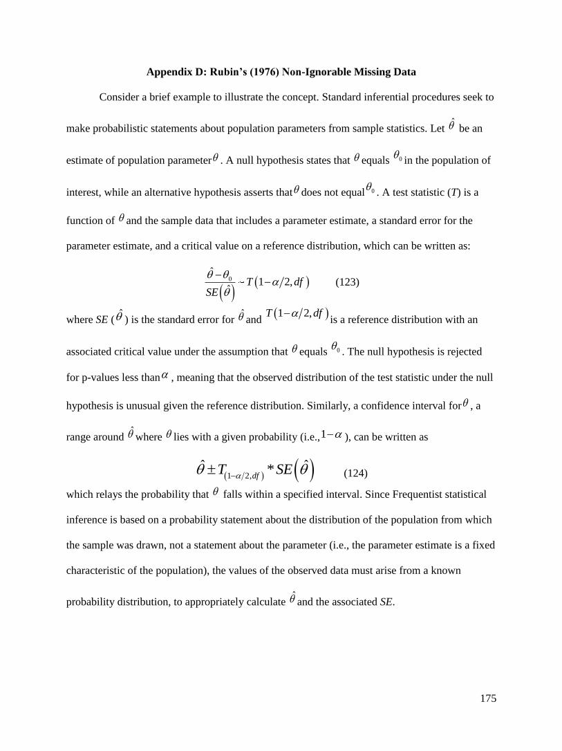
175

Appendix D: Rubin’s (1976) Non-Ignorable Missing Data

Consider a brief example to illustrate the concept. Standard inferential procedures seek to

make probabilistic statements about population parameters from sample statistics. Let be an

estimate of population parameter . A null hypothesis states that equals 0 in the population of

interest, while an alternative hypothesis asserts that does not equal 0 . A test statistic (T) is a

function of and the sample data that includes a parameter estimate, a standard error for the

parameter estimate, and a critical value on a reference distribution, which can be written as:

0

ˆ1 2,

ˆT df

SE

(123)

where SE ( ) is the standard error for and 1 2,T df

is a reference distribution with an

associated critical value under the assumption that equals 0 . The null hypothesis is rejected

for p-values less than , meaning that the observed distribution of the test statistic under the null

hypothesis is unusual given the reference distribution. Similarly, a confidence interval for , a

range around where lies with a given probability (i.e.,1 ), can be written as

1 2,ˆ ˆ*

dfT SE

(124)

which relays the probability that falls within a specified interval. Since Frequentist statistical

inference is based on a probability statement about the distribution of the population from which

the sample was drawn, not a statement about the parameter (i.e., the parameter estimate is a fixed

characteristic of the population), the values of the observed data must arise from a known

probability distribution, to appropriately calculate and the associated SE.

176

Appendix E: Demonstration of the EM Algorithm

To demonstrate the EM algorithm using the linear model equation, first recall the simple

regression equation (for the ith

observation, prediction of Yi by k variables in Xik):

0 1 1i i iY X e (125)

where β0 is the intercept, β1 signifies a slope with a predictor X and an associated error term e.



Y Xb e (126)

where Y is an (N × 1) vector that contains the dependent variable y, X is an (N × (k - 1)) design

matrix that contains a column of 1s and k – 1 columns of predictors, b is a (k × 1) vector of beta

weights, and e is an (N × 1) residual vector. When illustrated this formula becomes:

1 11 1

2 21 20

1

1

1 1 1 1

1

1

1

= +

N N N

N N k k N

Y X e

Y X e

Y X e

Y X b e

(127)

where 20,N e NN e I

and the first case is 1 0 1 11 1Y X e . Given the previous matrix

model, assume missing data on Y. More specifically, let Y1,...,Ym represent observed values

(Yobs), while Ym+1,…,Yp indicate missing values (Ymiss; see Figure 53).

Next, consider that Y = Xb + e can be rewritten to align Yobs with Xobs and Ymiss with Xmiss

such that the formula resembles:

177

111 1

1 0

1,11 11

1

1

1

1

1

1

= +

mm m

mm m

p pp

XY e

XY e

XY e

Y eX

Y X b e (128)

Now, the E-step can be directly implemented to estimate Ymiss via the least squares criterion by

minimizing (see Kutner, Nachtsheim, Neter, and Li, 2005):

2 2

, ,

1 1

( )N N


i i

e Y

x b Y X b Y X b e e

(129)

which can be written in relation to b that minimizes e e as:

1

obs obs obs obs

b X X X Y

(130)


squared residuals of a (m × 1) vector of Yobs (note that this is the mean of y without predictors in

the model) based on the associated (m × 1) vector of obsX. Once b is obtained it is then used to

predict the missing Ym+1,…,Yp values from the observed Xm+1,…,Xp values. To illustrate this

process, let example data from Blocks 4 and 5 of Table 1 be treated as Y and X, respectively, in

the forthcoming example; see Figure 53). Given the observed data (Yobs, Xobs) in Figure 53, the

next step is to apply the regression formula (see Equation 10) which can be demonstrated as:

178

1

1 1

0

1 1

1

12

2

2

2

22

1 1 1 1 1

1

1

1

N N

N N

x yb

x x x xb

x y

N x y yx x

x x xy xyx N

x y x xy

x y x xy

N xy x yN x x

-1b = X X X y

X X

22

22

2

2

22

2

22

1

1 cov( , )

var( )

1 1 cov( , )

var( )1 1

18.9971

N x x

N xy x y

N x x

x y x xyN

x yN x x y x

N interceptx

x y slopexy x yN N x

x xN N

1.968719.5650

6.76893.1499

1.9687 0.6250

3.1499

(131)

where Σ indicates summation, N is the observed sample size, cov denotes the covariance, var

represents the variance, b0 is the intercept parameter and b1 is the slope parameter (see Kutner,



The next step is to predict Ymiss (a missing value) from Xmiss (i.e., 20.22; an observed

value in X that corresponds to a missing value in Y; see Figure 3) using the regression weights

observed in b. The subsequent equation can be illustrated as:

179

6.7689 .6250 20.22

19.4065

miss

miss

Y

Y

(132)

To highlight the least squares criterion in this imputation method, notice that imputing 19.4065

for Ymiss and estimating Y = Xb + e produces the following set of residuals (see e vector below):

= +

21.15 1 21.14

19.41 1 20.22

20.40 1 20.81

19.96 1 20.69 6.769

17.21 1 19.59

19.29 1 18.33

16.91 1 15.40

18.06 1 20.34

Y X b e

1.22

0.00

0.66

0.28

0.625 1.85

0.93

0.18

1.42

(133)

where the imputed value (Ymiss) has a residual of zero (see Appendix QQQ for example R code).

The E-step uses Ymiss = 19.4065 in the y and

xy calculations; however, the E-step does not

literally fill in the missing value (e.g., Ymiss = 19.4065); rather this value is only referenced by the

following M-step (Enders, 2010). The ensuing M-step uses the now complete data to generate

estimates of the sufficient statistics as follows:

2

2

3.1499 1.7561

1.7561 2.0238

19.5650

19.0483

X YX

XY Y

X

Y

Σ

μ

(134)

where µ is a 2 × 1 column vector of means for X and Y, and Σ is a 2 × 2 covariance matrix.

These parameter estimates are then carried to the next E-Step as follows:

180

2

2

22

2

0

1

22

1

1 cov( , )

var( )

1 1 cov( , )

var( )1 1

1.756119.0483 19.5650

3.1498

1.7561

3.1498

x y x xyN

x yN x x y x

Nb interceptx

b x y slopexy x yN N x

x xN N

8.1404

0.5575

(135)

Again the procedure uses this information to predict Ymiss (a missing value) from Xmiss (i.e.,

20.22; an observed value in X that corresponds to a missing value in Y; see Figure 53) using the

regression weights observed in b. The subsequent equation can be illustrated as:

8.1404 .5575 20.22

19.4135

miss

miss

Y

Y

(136)

The following M-step again uses the estimate Ymiss = 19.4135 in the calculation of another set of

sufficient statistics and the process repeats until convergence (subsequent change in the MLE are

negligible).

Recall that the value of the log-likelihood function is a measure of joint likelihood of an

observed sample of data (represented by the individual data values) given the parameters in the

population covariance matrix Σ and the population mean vector µ where a smaller value

indicates better fit of the data to the population parameters. To demonstrate convergence let,

given 2

Y = 2.0 and Y = 19.5 so the likelihood estimates can be found by:

181

2

2

2

21.15 19.5.5

2.01

19.96 19.5.5

2.04

18.06 19.5.5

2.08

1( ) 0.143

2 (2.0)

1( ) 0.268

2 (2.0)

1( ) 0.168

2 (2.0)

f Y e

f Y e

f Y e

(137)

where Y1 is the first element (value) in the column matrix Y, Y2 is the second element, etc.

Notice that the estimated likelihood value for 2Y(i.e., Ymiss in Figure 3) would change depending

on which imputed value was used (e.g., 19.4065, 19.4135, etc.). Recall that the maximum

likelihood value is associated with the Yi value that is closest to Y given the other values and 2

Y

= 2.0. Likewise, the smallest log-likelihood value is considered the best estimate. Now consider

the sum of the log-likelihood (i.e., a measure of overall sample fit to µ; see appendix QQQ)

given each estimate of Ymiss for the first six iterations:

1

2

3

4

5

6

14.5797815

14.5794679

14.5794253

14.5794193

14.5794184

14.5794184

iteration

iteration

iteration

iteration

iteration

iteration

FML

FML

FML

FML

FML

FML

(138)

Note that the largest change occurred between the first and second iteration and each subsequent

iteration changed less until the change was negligible (e.g., beyond the seventh decimal place).

In this illustration, the EM algorithm would have converged in the sixth iteration provided the

convergence criteria were 1.0e-7

.

182

Appendix F: Discussion of FIML as a Direct ML Method

Consider how Finkbeiner (1979) applied FIML to the factor analysis model. Note that the

multivariate normal likelihood function can be expressed as L = likelihood function = function

(data, parameters) or more compactly as:

L ,f S Σ (139)

where S is the sample covariance and Σ is the population covariance matrix. From this

expression we can derive another equation that defines L as a function of the sample covariance

matrix S (as before) and the model-implied population covariance matrix Σ generated as a

function of the common factor model. That is, given that the common factor model for a

specified number of factors holds in the population the model implied covariance matrix can be

generated from the expression: Σ = ΛΛ +D

whereΛ represents factor loadings and D

indicates unique variances. Thus, the likelihood function can be re-expressed as:

L , ,f S Λ D

(140)

That is, the value of the likelihood function is dependent on the sample covariance matrix (which

is known) and the factor loadings and unique variances (which are not known). The goal is to

find best estimates of these population parameters. So, maximum likelihood estimates, Λ and Dψ

are chosen so that the likelihood function L = f(S, Σ) is maximized. Note that the mean vectors

were excluded from the previous formula for ease of presentation; however, they can be easily

incorporated.

The computational procedure for ML estimation works in general as follows: given S, the

parameters Λ and Dψ are estimated. From these estimates, a re-constructed covariance matrix

Σ = ΛΛ +D

is then generated. Afterwards, a value of the likelihood function, L = f(S, Σ) is

determined. Said differently, given S the task is to find Λ and Dψ so that the resulting Σ yields

183

the largest possible value of L = f(S, Σ). Therefore, the MLE estimation routine is directed to

locate values for Λ and Dψ so that the resulting covariance matrix Σ = ΛΛ +D

yields a

minimum value of MLE. When the optimal pattern of population estimates are found the

iterative optimization algorithm (i.e., sequence of a re-constructed covariance matrix

Σ = ΛΛ +D

) has found the best fit to the data (i.e., the highest log-likelihood; see Enders,

2010). In this way, the FIML procedure eliminates the need to then export the sufficient statistics

for further analyses (unlike the EM algorithm). As demonstrated above, this is accomplished by

building a model-implied covariance matrix that includes all the variables that are included in the

factor analysis model.

184

Appendix G: Discussion of Probability and Missing Data Mechanisms

To solidify the idea of probability distributions in this context, consider the diagram in

Figure 16 where Y represents the sampling space for four variables Y1 – Y4. That is, the variables

Y1 – Y4 each represent a possible event (occurrence) of Y and form four partitions of the total

sample space (represented by diagonal lines in Figure 16). For this example, let each patrician

(variable) be sampled at random with a .25 probability of being selected. That is, the probability

of Yi, denoted p(Yi), can be thought of as the frequency of drawing Yi (see Hays, 1994). Now, let

R be the occurrence of another event (i.e., the presence of missing data) which is depicted as a

circle in Figure 16. Let 15% of each randomly selected variable have missing data, so that there

is a .15 probability of the event “missing”.

Given the values of p(Y1), p(Y2), p(Y3), p(Y4), p(missing; R = 1), and p(not missing; R =

0) it is possible to determine the conditional probability of observing missing data on the thi

variable Y; however, the probability of each joint event (i.e., the occurrence of both Yi and R) is

dependent upon the independence of the events (Hays, 1994). Said differently, if the events

(probability distributions) are independent then missingness (denoted R) has absolutely nothing

to do with the variables Y1 – Y4. Otherwise, R is not simply a random sample of Y.

It is productive to consider an illustrative example of this idea. Consider Panel A of

Figure 54 where the two conditions, Yi and R, are independent. That is, the probability p(Y1 and

[R=1]) is equal to the product of the two marginal probabilities (.25 and .15, respectively).

Likewise, the probabilities for any of the other cells may be found by multiplying the associated

marginal probabilities (see Hays, 1994). Because these events are independent the probability of

missing data given any particular variable is as follows:

185

1

2

3

4

1 0.15

1 0.15

1 0.15

1 0.15

p R Y

p R Y

p R Y

p R Y

(141)

Hence, if the event Yi is independent of the event “missing data” the probability of the joint event

is found by p(Yi and “missing data”) = p(Yi) × p(R=1) = .25 × .15 = .034. So based on these

probabilities, the variable Yi is drawn with missing data in about 34 of 1000 random selections

(see Figure 54). Notice that the probability of missingness given Yi is constant and this value is

equal to the original probability of missingness, denoted p(R=1) = 0.15 in Figure 54. Visually,

the sampling space Y in Figure 16 shrinks to R as the variable Yi is completely unrelated. That is,

ignoring the diagonal partitions for Yi in the circle R leads to the probability of R (see Figure 54)

which can be expressed mathematically by:

( | ) ( ) 0.15p p R Y R (142)

where the probability of missingness is unrelated to the data. Now consider Panel B of Figure 54

where the two conditions Yi and R are not independent. That is, the probability p(Y1 and [R=1])

is not equal to the product of the two marginal probabilities such that:

1

2

3

4

1 0.24

1 0.08

1 0.12

1 0.16

p R Y

p R Y

p R Y

p R Y

(143)

Notice that the probability of missingness is dependent on Yi and is not equal to the original

probability of missingness. That is, R is not a random sample of Y, so the diagonal partitions for

Yi in the circle R remain and directly relate to the probability of missingness (see Figure 54).

Therefore, the sample space for R is associated with Y such that:

( | ) ( | )p pR Y R Y (144)

186

Said differently, the probability of missingness is dependent on the data. The idea that the data

provide information about the probability of missingness (i.e., causal relationships between

variables and R) is a key concept behind Rubin’s (1976) theory.

187

Appendix H: Demonstration of data augmentation in MI

To demonstrate the data augmentation algorithm using the linear model equation, first

consider a simple regression equation (for the ith

observation, prediction of Yi by k variables in

Xik) which can be written as:

0 1 1ˆi i iY X e (145)

where β0 is the intercept, β1 signifies a slope with a predictor X and an associated error term e.



Y Xb e (146)

where Y is an (N × 1) vector that contains the dependent variable y, X is an (N × (k - 1)) design

matrix that contains a column of 1s and k – 1 columns of predictors, b is a (k × 1) vector of beta

weights, and e is an (N × 1) residual vector. This formula can be explicitly illustrated as:

1 11 1

2 21 20

1

1

1 1 1 1

1

1

1

= +

N N N

N N k k N

Y X e

Y X e

Y X e

Y X b e (147)

where e ~ 20,N e NN I and the first case is 1 0 1 11 1Y X e . Given the previous matrix

equation, assume missing data on Y. More specifically, let Y1,...,Ym represent observed values

(Yobs), while Ym+1,…,Yp indicate missing values (Ymiss). Further, consider that Y = Xb + e can be

rewritten to align Yobs with Xobs and Ymiss with Xmiss such that the matrix expression resembles:

188

111 1

1 0

1,11 11

1

1

1

1

1

1

= +

mm m

mm m

p pp

XY e

XY e

XY e

Y eX

Y X b e

(148)

Now, the I-step can be directly implemented to estimate Ymiss via the least squares criterion by

minimizing the sum of square error terms such that (see Kutner, Nachtsheim, Neter, and Li,

2005):

2 2

, ,

1 1

( )N N


i i

e Y

x b Y X b Y X b e e (149)

which can be written in relation to b that minimizes e e as:

1

obs obs obs obs

b X X X Y (150)


squared residuals of a (m × 1) vector of Yobs (note that this is the mean of y without predictors in

the model) based on the associated (m × 1) vector of obsX . Once b is obtained it is then used to

predict the missing Ym+1,…,Yp values from the observed Xm+1,…,Xp values. To illustrate this

process, consider the example data in Figure 26 for Y and X, respectively. Given the observed

data (i.e., Yobs, Xobs), the next step is to apply the regression formula, which can be demonstrated

as:

189

1

1 1

0

1 1

1

12

2

2

2

22

1 1 1 1 1

1

1

1

N N

N N

x yb

x x x xb

x y

N x y yx x

x x xy xyx N

x y x xy

x y x xy

N xy x yN x x

-1b = X X X y

X X

22

22

2

2

22

2

22

1

1 cov( , )

var( )

1 1 cov( , )

var( )1 1

18.9971

N x x

N xy x y

N x x

x y x xyN

x yN x x y x

N interceptx

x y slopexy x yN N x

x xN N

1.968719.5650

6.76893.1499

1.9687 0.6250

3.1499

(151)

where Σ indicates summation, N is the observed sample size, “cov” denotes the covariance, “var”

represents the variance, b0 is the intercept parameter and b1 is the slope parameter (see Kutner,



The next step is to predict Ymiss (a missing value) from Xmiss (i.e., 20.22; an observed

value in X that corresponds to a missing value in Y; see Figure 26) using the regression weights

observed in the vector b. The subsequent equation can be illustrated as:

6.7689 .6250 20.22

19.4065

miss

miss

Y

Y

(152)

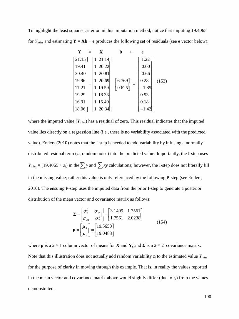
190

To highlight the least squares criterion in this imputation method, notice that imputing 19.4065

for Ymiss and estimating Y = Xb + e produces the following set of residuals (see e vector below):

= +

21.15 1 21.14

19.41 1 20.22

20.40 1 20.81

19.96 1 20.69 6.769

17.21 1 19.59

19.29 1 18.33

16.91 1 15.40

18.06 1 20.34

Y X b e

1.22

0.00

0.66

0.28

0.625 1.85

0.93

0.18

1.42

(153)

where the imputed value (Ymiss) has a residual of zero. This residual indicates that the imputed

value lies directly on a regression line (i.e., there is no variability associated with the predicted

value). Enders (2010) notes that the I-step is needed to add variability by infusing a normally

distributed residual term (zi; random noise) into the predicted value. Importantly, the I-step uses

Ymiss = (19.4065 + zi) in the y and xy calculations; however, the I-step does not literally fill

in the missing value; rather this value is only referenced by the following P-step (see Enders,

2010). The ensuing P-step uses the imputed data from the prior I-step to generate a posterior

distribution of the mean vector and covariance matrix as follows:

2

2

3.1499 1.7561

1.7561 2.0238

19.5650

19.0483

X YX

XY Y

X

Y

Σ

μ

(154)

where µ is a 2 × 1 column vector of means for X and Y, and Σ is a 2 × 2 covariance matrix.

Note that this illustration does not actually add random variability zi to the estimated value Ymiss

for the purpose of clarity in moving through this example. That is, in reality the values reported

in the mean vector and covariance matrix above would slightly differ (due to zi) from the values

demonstrated.

191

During the next step, Monte Carlo simulation is used to generate new parameter values

for µ and Σ that differ randomly from the parameters used in the initial I-step (see Enders, 2010).

These parameter estimates are then carried to the next I-Step as follows:

2

2

22

2

0

1

22

1

1 cov( , )

var( )

1 1 cov( , )

var( )1 1

1.756119.0483 19.5650

3.1498

1.7561

3.1498

x y x xyN

x yN x x y x

Nb interceptx

b x y slopexy x yN N x

x xN N

8.1404

0.5575

(155)

Again the procedure uses this information to predict Ymiss (a missing value) from Xmiss (i.e.,

20.22; an observed value in X that corresponds to a missing value in Y) using the regression

weights observed in b. The subsequent equation can be illustrated as:

8.1404 .5575 20.22

19.4135

miss

miss

Y

Y

(156)

The following M-step again uses the estimate Ymiss = (19.4135 + zi) in the calculation of another

set of sufficient statistics and the process repeats a large number of times. Unlike the EM

algorithm, this procedure does not converge on a set of most likely values (as each of these

iterations involves a random perturbation). Rather, each m imputed dataset is saved after a given

set of I-step to P-step cycles. For example, suppose that the m = 1 imputed data set is the imputed

data at the 200th

P-step, and the m = 2 dataset is the imputed data at the 300th

P-step, etc. (i.e., the

default criteria in SAS, for example, is 200 burn-in iterations before the first imputation and 100

iterations between imputations; see SAS Institute Inc., 2011 for details).

192

Appendix I: Syntax Guide to Using PCA Auxiliary Variables

Preliminaries

This appendix outlines a method of using principal component analysis (PCA) to obtain

auxiliary variables for large data sets. Typically, auxiliary variables are not the focus of an

analysis but are instead used to inform the missing data handling procedure (e.g., FIML, MI) by

adding information about why a particular variable has missing data or describing the probability

that a particular case has missing data. Therefore, auxiliary variables support the missing at

random assumption and are used to reduce bias and decrease standard errors (Collins, Schafer, &

Kam, 2001; Enders & Peugh, 2004; Graham, 2003).

Researchers suggest an “inclusive strategy” where as many auxiliary variables are

included as possible (see Enders, 2010). However, it is often difficult to include large numbers of

auxiliary variables without having estimation problems; especially when the auxiliary variables

also have missing data. Large data projects can present a challenge because it is possible to have

hundreds of potential auxiliary variables to choose from.

The current method uses PCA to reduce the dimensionality of the data set. A new set of

uncorrelated variables are created (e.g., principal components) that contain all the useful

information in the original data set. These principal components are then used to inform the

missing data handling procedure. This guide illustrates the application of these PCA auxiliary

variables to both FIML and MI methods.

Step One: Obtain principal components from the data set

1) Perform a single imputation for the entire data set

The SAS Proc MI syntax will look something like this:

Proc mi data=sample out=outmi nimpute=1 seed=461981;

em maxiter=1000;

mcmc chain=multiple initial=em (maxiter = 1000);

run;

*For Proc mi options see: http://support.sas.com/onlinedoc/913/docMainpage.jsp;

At this step the data are all imputed a single time.

193

a) Note. Like other multivariate methods, PCA requires complete data.

2) Impute at the level of the aggregate scales.


Proc mi data=sample out=outmi nimpute=1 seed=761253;

em maxiter=1000;


var ScaleA ScaleB ScaleC ScaleD ScaleE ScaleF ScaleG ScaleH ScaleI ScaleJ;

run;


At this step the scales now have NO missing data but the items still contain missing data

3) Use the imputed scales as anchors to impute missing data in the items in a sequential

process

Now the key is to put the right variables into the variable list for estimating the missing data:

Proc mi data=outmi out=outmi......;

var ScaleA ScaleB ScaleC ScaleD ScaleE ScaleF ScaleG ScaleH ScaleI

j1 j2 j3 j4 j5 j6 j7 j8 j9;

* At this step ScaleJ is not in the list but the items for ScaleJ are now imputed;

* ScaleJ needs to be removed because it is a linear combination of its items;


var ScaleA ScaleB ScaleC ScaleD ScaleE ScaleF ScaleG ScaleH ScaleJ

i1 i2 i3 i4 i5 i6 i7 i8;

* At this step ScaleI is not in the list but the items for ScaleI are now imputed;


var ScaleA ScaleB ScaleC ScaleD ScaleE ScaleF ScaleG ScaleI ScaleJ

h1 h2 h3 h4 h5 h6 h7 h8 h9 h10;

* At this step ScaleH is not in the list but the items for ScaleH are now imputed;


var ScaleA ScaleB ScaleC ScaleD ScaleE ScaleF ScaleH ScaleI ScaleJ

g1 g2 g3 g4 g5 g6 g7 g8 g9 g10;

* At this step ScaleG is not in the list but the items for ScaleG are now imputed;


var ScaleA ScaleB ScaleC ScaleD ScaleE ScaleG ScaleH ScaleI ScaleJ

f1 f2 f3 f4 f5 f6 f7 f8 f9 f10;

* At this step ScaleF is not in the list but the items for ScaleF are now imputed;


var ScaleA ScaleB ScaleC ScaleD ScaleF ScaleG ScaleH ScaleI ScaleJ

e1 e2 e3 e4 e5 e6 e7 e8 e9 e10;

* At this step ScaleE is not in the list but the items for ScaleE are now imputed;

194


var ScaleA ScaleB ScaleC ScaleE ScaleF ScaleG ScaleH ScaleI ScaleJ

d1 d2 d3 d4 d5 d6 d7 d8 d9 d10;

* At this step ScaleD is not in the list but the items for ScaleD are now imputed;


var ScaleA ScaleB ScaleD ScaleE ScaleF ScaleG ScaleH ScaleI ScaleJ

c1 c2 c3 c4 c5 c6 c7 c8 c9 c10;

* At this step ScaleC is not in the list but the items for ScaleC are now imputed;


var ScaleA ScaleC ScaleD ScaleE ScaleF ScaleG ScaleH ScaleI ScaleJ

b1 b2 b3 b4 b5 b6 b7 b8 b9 b10;

* At this step ScaleB is not in the list but the items for ScaleB are now imputed;


var ScaleB ScaleC ScaleD ScaleE ScaleF ScaleG ScaleH ScaleI ScaleJ

a1 a2 a3 a4 a5 a6 a7 a8 a9 a10;

* At this step ScaleA is not in the list but the items for ScaleA are now imputed;

At this point ALL of the items are imputed.

Method Two:

1) Do a principal components analysis of the items on the dataset and output the

meaningful components as component scores.

The SAS Proc Princomp syntax ( Proc Factor may also be used) will look something like this:

Proc princomp data=sample out=Prin;

var a1-a10 b1-b10 c1-c10 d1-d10 e1-e10 f1-f10 g1-g10 h1-h10 i1-i8 j1-j9;

run;

*For Proc princomp options: http://support.sas.com/onlinedoc/913/docMainpage.jsp;

In this example, let’s assume that the first 12 components accounted for a meaningful amount of

variance and any more components would not yield much more reliable information.

2) Estimate any missing data on the component scores


Proc mi data=Prin out=outmi nimpute=1 seed=761253;

em maxiter=1000;


var Component1-Component12;

run;


At this step, the component scores now have NO missing data but the items still contain

195

missingness.

3) Use the estimated component scores as anchors to estimate the missing data in the

items on the dataset.


var Component1-Component12 a1-a10 b1-b10;

* At this step we plug approximately 20 items into the variable list to estimate

their missing values;


var Component1-Component12 c1-c10 d1-d10;

* At this step we plug in approximately 20 more items into the list to estimate



var Component1-Component12 e1-e10 f1-f10;




var Component1-Component12 g1-g10 h1-h10;




var Component1-Component12 i1-i8 j1-j9;

* At this step we plug the remaining items to estimate their missing values;

At this point ALL of the items are imputed.

What about Multiple Imputations:

1) Change the number of imputations option (nimpute= ) in the Proc MI syntax


Proc mi data=outmi out=outmi nimpute=20......;

var ScaleA ScaleB ScaleC ScaleD ScaleE ScaleF ScaleG ScaleH ScaleI

j1 j2 j3 j4 j5 j6 j7 j8 j9;

* At this step ScaleJ is not in the list but the items for ScaleJ are now imputed;

Proc mi data=outmi out=outmi nimpute=20......;

var ScaleA ScaleB ScaleC ScaleD ScaleE ScaleF ScaleG ScaleH ScaleJ

i1 i2 i3 i4 i5 i6 i7 i8;

* At this step ScaleI is not in the list but the items for ScaleI are now imputed;

Notes. Multiple imputations should be carried out during Step 3 of the previous two

196

examples. It is not suggested to impute the initial aggregate scales or the initial

component scores as in Step 2. Therefore, multiple imputations are created only for the

imputed items.

The input and output datasets in the SAS syntax do not change with each

imputation step; this stacks the imputed datasets on top of each other 1 – 20. If the

original dataset contained 200 observations then the new data set with 20 imputations

will contain 4000 observations with the 201st observation being the first observation in

the 2nd

imputation. SAS will create a new variable called “_imputation_” with a value of

1 for the first imputation, 2 for the second imputation, and so on to a value of 20 for the

last imputation.

At this point ALL of the items are imputed 20 times.

For additional information regarding further analysis of a dataset with multiple imputations in

LISREL see the Rubin’s Rules Pooler for LISREL Estimates:

http://www.quant.ku.edu/resources/tools.html

Helpful SAS code for the aggregate scale method:

a) Creating a scale based on item means.

The SAS Proc Standard syntax will look something like this:

Data sampleNew ; set sample ;

ScaleA = mean(of a1 a2 a3 a4 a5 a6 a7 a8 a9 a10);

ScaleB = mean(of b1 b2 b3 b4 b5 b6 b7 b8 b9 b10);

... ;

run;

b) Standardize before imputing (when a scale is created from item SUM).

The SAS Proc Standard syntax will look something like this:

Proc standard data=sample mean=0 std=1 out=zsample;

var ScaleA ScaleB ScaleC ScaleD ScaleE ScaleF ScaleG ScaleH ScaleI ScaleJ;

run;

http://www.quant.ku.edu/resources/tools.html

197

Table 1 Data from an exemplar randomized block design taken from Allan and Wishart.

Data from an exemplar randomized block design taken from Allan and Wishart (1930).

Note. “–“denotes a missing value. The data in this example represent protein percentage in peas

across nine treatments and eight replicates.

Table 1.

Exemplar data from a randomized block design taken from Allan and Wishart (1930).

Block 1 2 3 4 5 6 7 8 9 Totals

A 15.96 16.80 19.08 21.15 21.14 23.02 20.60 26.34 25.32 189.41

B 21.96 24.44 26.33 ― 20.22 20.87 19.21 20.04 21.30 174.37

C 18.78 18.36 19.40 20.40 20.81 23.77 17.24 18.00 20.46 177.22

D 20.18 20.52 20.42 19.96 20.69 20.90 21.68 21.90 20.68 186.93

E 16.20 16.90 19.81 17.21 19.59 21.22 18.72 20.04 19.02 168.71

F 18.64 20.33 22.71 19.29 18.33 19.06 20.04 21.31 22.19 181.90

G 18.89 23.60 22.42 16.91 15.40 17.00 16.71 18.02 19.84 168.79

H 19.22 20.47 20.98 18.06 20.34 21.38 16.83 15.66 17.21 170.15

Total 149.83 161.42 171.15 132.98 156.52 167.22 151.03 161.31 166.02 1417.48

Mean 18.73 20.18 21.39 19.00 19.57 20.90 18.88 20.16 20.75 19.96

Treatments

198

Table 2 Iterative solutions for a set of linear equations.

Iterative solutions for a set of linear equations.

199

Table 3 Exemplar data illustrating MCAR, MAR and MNAR missing data mechanisms.

Exemplar data illustrating MCAR, MAR and MNAR missing data mechanisms.

Note. The mean ( 2y ), standard deviation (2ySD ), and correlation (

1 2y yr ) are M = -0.04, SD = .89,

r = .67 among the complete data example; are M = -0.02, SD = 1.00, r = .69 among the MCAR

200

data example; are M = 0.54, SD = .77, r = .19 among the MAR data example; and are M = 0.71,

SD = .51, r = .40 among the MNAR data example.

201

Table 4 Simulation results showing the impact of omitting a cause or correlate of missing

Simulation results showing the impact of omitting a cause or correlate of missingness.

Note. ρA,Y denotes the population correlation between Y and the omitted auxiliary variable; ρX,Y

denotes the correlation between X and Y; μY is the mean of Y and 2

Y is the variance of Y.

202

Table 5 Simulation results showing the influence of auxiliary variables to improve

Simulation results showing the influence of auxiliary variables to improve parameter estimation

in an MNAR situation.




203

Table 6 Simulation results showing the bias associated with ignoring a non-linear cause

Simulation results showing the bias associated with ignoring a non-linear cause of missingness.




204

Table 7 Simulated data for PCA examples.

Simulated data for PCA examples.

205

Tab

le 8

Monte

Carl

o s

imula

tion s

tudie

s publi

shed

in t

he

soci

al

scie

nce

s on t

he

topic

Monte

Carl

o s

imula

tion s

tudie

s publi

shed

in t

he

soci

al

scie

nce

s on t

he

topic

of

mis

sing d

ata

handli

ng.

206

Table 9 Raw ECI key skills data in 3-month intervals from 9 – 36 months.

Raw ECI key skills data in 3-month intervals from 9 – 36 months.

Gestures Vocalizations Single Words Multiple Words

Age Mean (SE) Mean (SE) Mean (SE) Mean (SE)

9 9.49 (.34) 12.79 (.56) 0.09 (.02) ---

n = 287 n = 285 n = 285 n = 285

12 10.25 (.38) 22.34 (.79) 0.8 (.11) 0.03 (.02)

n = 285 n = 285 n = 285 n = 79

15 12.39 (.42) 22.74 (.77) 2.8 (.26) 0.11 (.03)

n = 295 n = 294 n = 289 n = 293

18 10.92 (.42) 23.3 (.64) 6.66 (.47) 0.56 (.08)

n = 295 n = 296 n = 289 n = 288

21 10.16 (.39) 21.55 (.77) 12.92 (.69) 2.22 (.24)

n = 275 n = 276 n = 276 n = 269

24 10.17 (.42) 19.14 (.75) 17.87 (.80) 5.91 (.49)

n = 258 n = 257 n = 256 n = 250

27 9.71 (.43) 16.74 (.77) 20.51 (.78) 13.57 (.86)

n = 256 n = 258 n = 258 n = 259

30 8.86 (.42) 15.19 (.82) 20.7 (.74) 18.18 (.99)

n = 224 n = 222 n = 223 n = 225

33 8.75 (.44) 12.82 (.71) 20.67 (.72) 20.99 (1.03)

n = 224 n = 223 n = 225 n = 226

36 7.4 (.53) 11.78 (.77) 19.59 (.94) 25.67 (1.54)

n = 127 n = 127 n = 127 n = 128

Note. Age reflects average months since birth; SE represents the standard error; n denotes the

sample size associated with each mean and standard deviation. Multiple Words were not

assessed at 9 months due to developmental limitations.

207

Tab

le 1

0 M

onte

Carl

o s

imula

tion r

esult

s sh

ow

ing t

he

impact

of

PC

AA

UX

and A

UX

Monte

Carl

o s

imula

tion r

esu

lts

show

ing t

he

impact

of

PC

AA

UX

and A

UX

on p

ara

met

er e

stim

ati

on r

aw

bia

s, s

tandard

ized

bia

s, a

nd p

erce

nt

bia

s acr

oss

vari

ous

sam

ple

siz

es w

hen

mis

singnes

s is

rel

ate

d t

o a

60%

MA

R m

issi

ng d

ata

rate

and a

popula

tion a

ssoci

ati

on o

f ρ =

.60 a

mong t

he

auxi

liary

vari

ab

les.

208

Tab

le 1

1 M

onte

Carl

o s

imula

tion r

esult

s sh

ow

ing t

he

impa

ct o

f P

CA

AU

X a

nd A

UX

Monte

Carl

o s

imula

tion r

esult

s sh

ow

ing t

he

impact

of

PC

AA

UX

and A

UX

on p

ara

met

er e

stim

ati

on r

aw

bia

s, s

tand

ard

ized

bia

s, a

nd p

erce

nt

bia

s acr

oss

vari

ous

sam

ple

siz

es w

hen

mis

singnes

s is

rel

ate

d t

o a

non

-lin

ear

pro

cess

wit

h a

60%

MA

R

mis

sing d

ata

rate

and a

popula

tion a

ssoci

ati

on o

f ρ =

.60 a

mong t

he

auxi

liary

vari

ab

les.

209

Table 12 Monte Carlo simulation results showing the impact of PCAAUX and AUX

Monte Carlo simulation results showing the impact of PCAAUX and AUX (with non-linear

information) on parameter estimation raw bias, standardized bias, and percent bias across

various sample sizes when missingness is related to a non-linear process with a 60% MAR

missing data rate and a population association of ρ = .60 among the auxiliary variables.

Mechanism Raw Std. Percent Raw Std. Percent

Parameter Est. Bias Bias Bias Est. Bias Bias Bias

Non-linear MAR

Y with X (ρX,Y) 0.300 0.295 -0.005 -0.005 -1.695% 0.290 0.010 0.080 3.367%

Mean Y (μY) 0.000 -0.001 -0.001 -0.001 -0.006 0.006 0.045

Variance Y (σ2Y) 1.000 0.992 -0.008 -0.005 -0.794% 1.013 -0.013 -0.073 -1.340%

Non-linear MAR

Y with X (ρX,Y) 0.300 0.301 0.001 0.001 0.395% 0.299 0.001 0.025 0.233%

Mean Y (μY) 0.000 0.000 0.000 0.000 -0.002 0.002 0.024

Variance Y (σ2

Y) 1.000 0.996 -0.004 -0.003 -0.392% 0.997 0.003 0.030 0.320%

Non-linear MAR

Y with X (ρX,Y) 0.300 0.300 0.000 0.000 -0.118% 0.300 0.000 -0.005 -0.133%

Mean Y (μY) 0.000 0.002 0.002 0.002 0.001 -0.001 -0.020

Variance Y (σ2Y) 1.000 0.999 -0.001 -0.001 -0.091% 0.998 0.002 0.034 0.180%

Non-linear MAR

Y with X (ρX,Y) 0.300 0.300 0.000 0.000 0.072% 0.300 0.001 0.015 0.167%

Mean Y (μY) 0.000 0.000 0.000 0.000 0.000 0.000 -0.008

Variance Y (σ2Y) 1.000 0.999 -0.001 -0.001 -0.115% 0.998 0.002 0.043 0.200%

N = 800

N = 1000

PCA Auxiliary Variable All Possible Auxiliary Variables (INT)

N = 75

N = 200

210

Table 13 Relative Efficiency of correlation parameter estimate between X and Y

Relative Efficiency of correlation parameter estimate between X and Y by sample size, MCAR

missing data rate and association strength between the variable with missingness and the

auxiliary variables.

Percent Missing

N 10% 20% 30% 40% 50% 60% 70%

80%

ρX,Y = .10

100 1.002 1.005 1.008 1.008 1.015 1.022 1.026 1.028

400 1.001 1.001 1.001 1.000 0.999 0.999 0.999 0.999

1000 0.999 0.999 0.999 0.999 0.999 0.999 0.999 0.999

ρX,Y = .30

100 1.002 1.007 1.015 1.018 1.027 1.031 1.033 1.038

400 1.002 1.004 1.007 1.009 1.012 1.019 1.022 1.023

1000 1.001 1.004 1.006 1.008 1.011 1.016 1.019 1.021

ρX,Y = .60

100 1.014 1.034 1.065 1.100 1.145 1.222 1.263 1.289

400 1.016 1.034 1.060 1.097 1.143 1.210 1.231 1.240

1000 1.015 1.026 1.037 1.096 1.117 1.155 1.193 1.206

Note. Values greater than 1.0 indicate that PCAAUX estimates are more efficient.

211

Tab

le 1

4 M

ult

iple

im

puta

tion o

f E

CI

key

skil

ls d

ata

usi

ng n

o a

uxi

liary

vari

ab

les.

Mult

iple

Im

puta

tion o

f E

CI

key

skil

ls d

ata

usi

ng n

o a

uxi

liary

vari

ab

les.

212

Tab

le 1

5 M

ult

iple

im

puta

tion o

f E

CI

key

skil

ls d

ata

usi

ng t

he

AU

X m

ethod

Mult

iple

Im

puta

tion

of

EC

I ke

y sk

ills

data

usi

ng t

he

AU

X m

ethod (

all

poss

ible

auxi

liary

vari

ab

les)

.

213

Tab

le 1

6 M

ult

iple

Im

puta

tion o

f E

CI

key

skil

ls d

ata

usi

ng t

he

PC

A a

uxi

liary

vari

ab

les.

Mult

iple

Im

puta

tion o

f E

CI

key

skil

ls d

ata

usi

ng t

he

PC

A a

uxi

liary

vari

ab

les.

214

Table 17 A Demonstration of marginal means estimation for the main effect of B.

A Demonstration of marginal means estimation for the main effect of B with complete data.

Note. Each observed value is written in terms of the ANOVA model parameters where µ

represents a grand mean, αj is the effect of the jth


level of B

(excluding (αβ)jk and εijk for simplicity).

215

Table 18 A Demonstration of marginal means estimation for the main effect of B.

A Demonstration of marginal means estimation for the main effect of B with incomplete data.

Note. Each observed value is written in terms of the ANOVA model parameters where µ

represents a grand mean, αj is the effect of the jth


level of B

(excluding (αβ)jk and εijk for simplicity).

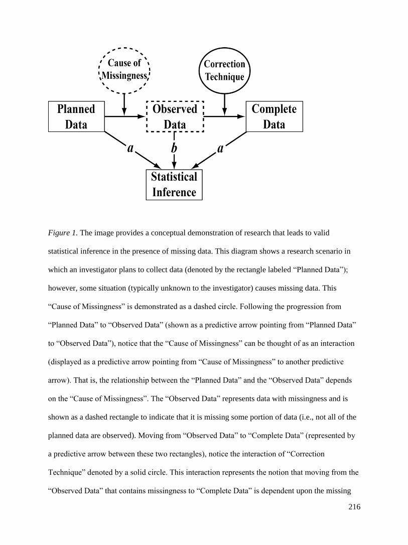
216

Figure 1. The image provides a conceptual demonstration of research that leads to valid

statistical inference in the presence of missing data. This diagram shows a research scenario in

which an investigator plans to collect data (denoted by the rectangle labeled “Planned Data”);

however, some situation (typically unknown to the investigator) causes missing data. This

“Cause of Missingness” is demonstrated as a dashed circle. Following the progression from

“Planned Data” to “Observed Data” (shown as a predictive arrow pointing from “Planned Data”

to “Observed Data”), notice that the “Cause of Missingness” can be thought of as an interaction

(displayed as a predictive arrow pointing from “Cause of Missingness” to another predictive

arrow). That is, the relationship between the “Planned Data” and the “Observed Data” depends

on the “Cause of Missingness”. The “Observed Data” represents data with missingness and is

shown as a dashed rectangle to indicate that it is missing some portion of data (i.e., not all of the

planned data are observed). Moving from “Observed Data” to “Complete Data” (represented by

a predictive arrow between these two rectangles), notice the interaction of “Correction

Technique” denoted by a solid circle. This interaction represents the notion that moving from the

“Observed Data” that contains missingness to “Complete Data” is dependent upon the missing

217

data handling technique utilized by the investigator. Conceptually, the “Complete Data”

rectangle in this demonstration consists of data that would have been obtained had there been no

missing values (i.e., the origina l “Planned Data”). Said differently, the “Correction Technique”

represents a missing data handling technique used to infer the complete data for subsequent

statistical modeling. Now, consider that the statistical inference implied from the “Planned Data”

(represented by a predictive arrow pointing from “Planned Data” to “Statistical Inference”)

should be equivalent to that implied from the complete data (denoted “a”). Additionally, the

statistical inference implied from deletion methods (i.e., failure to progress to complete data) is

likely to be biased (denoted “b”).

218

(A) Distribution with Y = 0,2

Y = 1.5 (B) Distribution with Y = 1.0,2

Y = 1.5

Figure 2. A graphical representation of the relationship between a sampling density (n = 5) and

two possible values of . The figure depicts that the population estimate = 0.0 is more

reasonable than population estimate = 1.0 given the observed sample from a normal

distribution.

219

Figure 3. A plot of the likelihood values as a function of various population means ranging from

Y = -3.0 to Y = 3.0. The image illustrates that the population estimate = 0.0 is most likely

(i.e., maximum likelihood) given the observed sample.

220

Figure 4. A plot of the log-likelihood values as a function of various population means ranging

from Y = -3.0 to Y = 3.0. The image illustrates that the population estimate = 0.0 is most

likely (i.e., minimum log-likelihood) given the observed sample.

221

Figure 5. A plot of the log-likelihood values as a function of various population variances

ranging from 2

Y = 0.12 to 2

Y = 1.32. The image illustrates that the population estimate2

Y = 0.48

is most likely (i.e., minimum log-likelihood) given the observed sample.

222

Figure 6. A close up view of the peak of the likelihood function used to demonstrate MLE

precision where the range of2

Y = 0.36 – 0.60 seem nearly as likely as 2

Y = 0.48, the maximum

likelihood variance estimate.

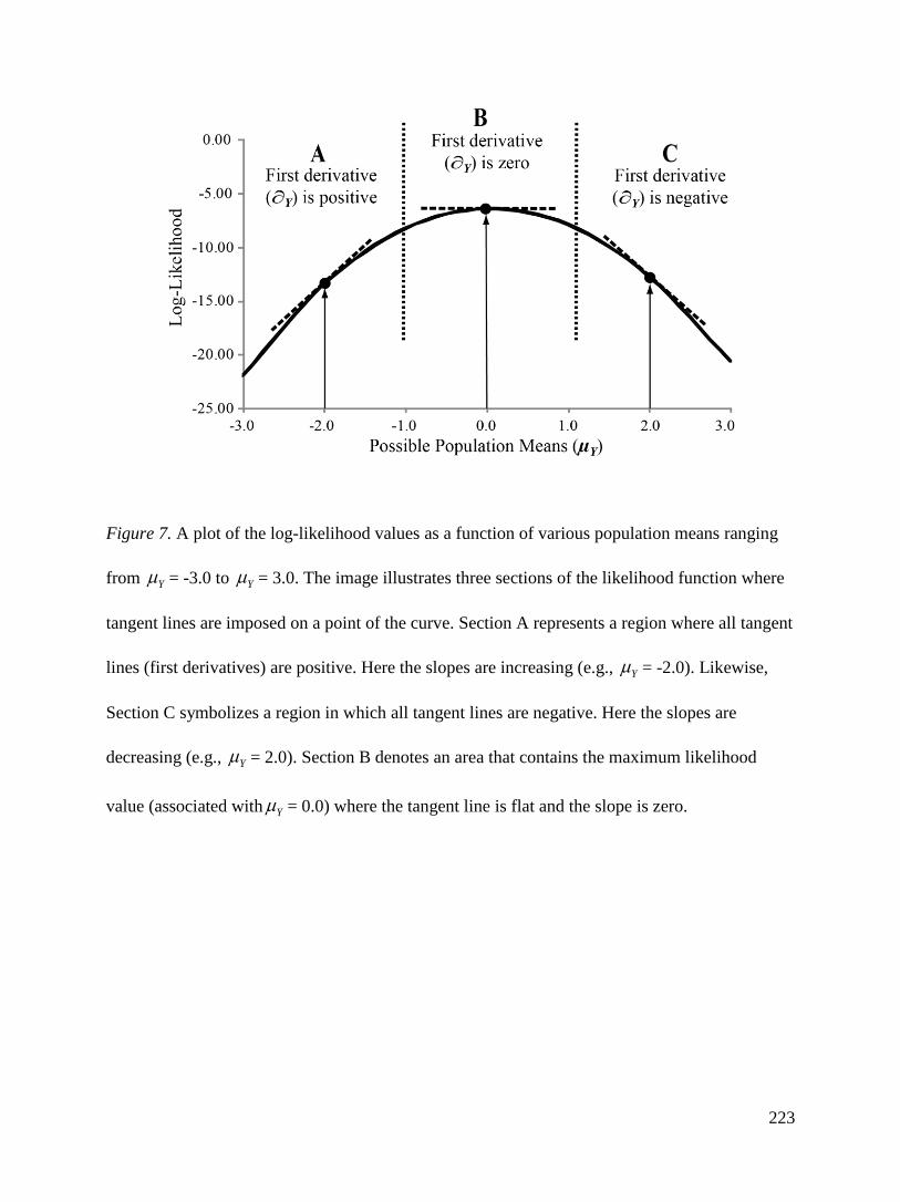
223


from Y = -3.0 to Y = 3.0. The image illustrates three sections of the likelihood function where

tangent lines are imposed on a point of the curve. Section A represents a region where all tangent

lines (first derivatives) are positive. Here the slopes are increasing (e.g., Y = -2.0). Likewise,

Section C symbolizes a region in which all tangent lines are negative. Here the slopes are

decreasing (e.g., Y = 2.0). Section B denotes an area that contains the maximum likelihood

value (associated with Y = 0.0) where the tangent line is flat and the slope is zero.

224


from Y = -3.0 to Y = 3.0 (top). This image explicitly illustrates the first derivatives of Y = -

2.0, Y = 0.0, and Y = -2.0 in relation to the likelihood function (calculated from equation 19). A

specific plot of the derivative regression line related to the likelihood function (bottom). The

image illustrates the relationship between the likelihood function and the first derivatives. Note

that the regression line transitions from positive values to negative values as it crosses the point

of maximum likelihood.

225

Figure 9. A three-dimensional plot of a bivariate normal probability distribution with X and Y

where the density function ( , )f X Y represents the height of the probability surface.

226

Figure 10. Illustration of Mahalanobis distance (denoted by the correlation ellipse) in a three-

dimensional scatter plot where point A and point B are the same distance from point C, the

multivariate centroid.

227

Figure 11. Illustration of missing data patterns where n is the number of i cases observed on Y

but not on X, s represents i + 1 to j cases that are observed on both X and Y, and m signifies j + 1

to k cases observed on X but not on Y.

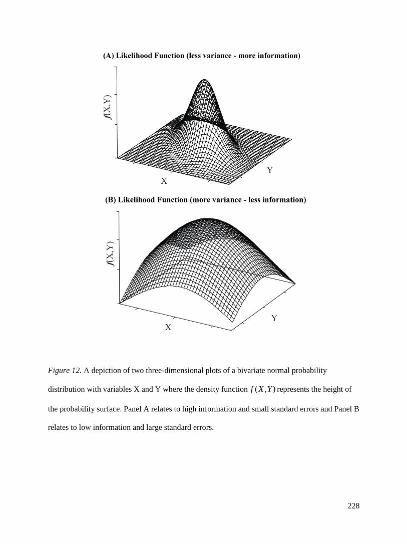
228

Figure 12. A depiction of two three-dimensional plots of a bivariate normal probability

distribution with variables X and Y where the density function ( , )f X Y represents the height of

the probability surface. Panel A relates to high information and small standard errors and Panel B

relates to low information and large standard errors.

229

Fig

ure

13. A

gra

phic

al d

epic

tion o

f th

e lo

g-l

ikel

ihood v

alues

as

a fu

nct

ion

of

var

ious

popula

tion m

eans

ran

gin

g f

rom

μY =

-3

.0 t

o μ

Y

= 3

.0 (

top o

f pan

els

A a

nd B

). T

his

im

age

expli

citl

y i

llust

rate

s th

e fi

rst

der

ivat

ives

of

μY =

-2.0

, μ

Y =

0.0

, an

d μ

Y =

-2.0

in r

elat

ion t

o

the

likel

ihood f

unct

ion (

calc

ula

ted f

rom

equat

ion 1

9)

for

two r

andom

sam

ple

s w

ith t

he

sam

e m

ean;

how

ever

, P

anel

B c

orr

esponds

to

a sa

mple

wit

h a

var

iance

that

is

2.5

tim

es l

arger

than

the

sam

ple

dat

a il

lust

rate

d i

n P

anel

A. T

he

imag

e il

lust

rate

s tw

o l

ikeli

ho

od

fun

ctio

ns

that

est

imat

e th

e sa

me

popula

tion m

ean (

e.g.,

μY =

0.0

) but

var

y i

n t

he

pre

cisi

on

of

the

par

amet

er e

stim

ate

(rat

e o

f ch

ang

e o

f

the

firs

t der

ivat

ives

). N

oti

ce t

hat

the

slopes

dem

on

stra

ted i

n P

anel

B a

re 2

.5 t

imes

sm

alle

r th

an t

he

corr

espondin

g s

lopes

in

Pan

el A

.

230

18 111 12 13 14 15

26 27 221 22 23 24

36 38 331 32 33

6 7 81 2 3 4 5

Incomplete Data Matrix

p

p

p

i i ii i i i i

y yy y y y y

y y yy y y y

y y yy y y

y y yy y y y y

Y participants

variables

Missingness Indicator Matrix

1 1 1 1 1

1

ip

N

y

p

R

1

2

3

6 7 81 2 3 4 5

0 0 1

1 1 01 1 1 0

1 0 11 1 1 0 0 participants

variables

p

p

p

i i i ipi i i i i

r

r

r N

r r r rr r r r r

p

Figure 14. Illustration of an incomplete data matrix Y where missingness is denoted by “−” and

a missingness indicator matrix R where missingness is denoted by “0”. Note that the matrix R

has the same dimensions as the matrix Y.

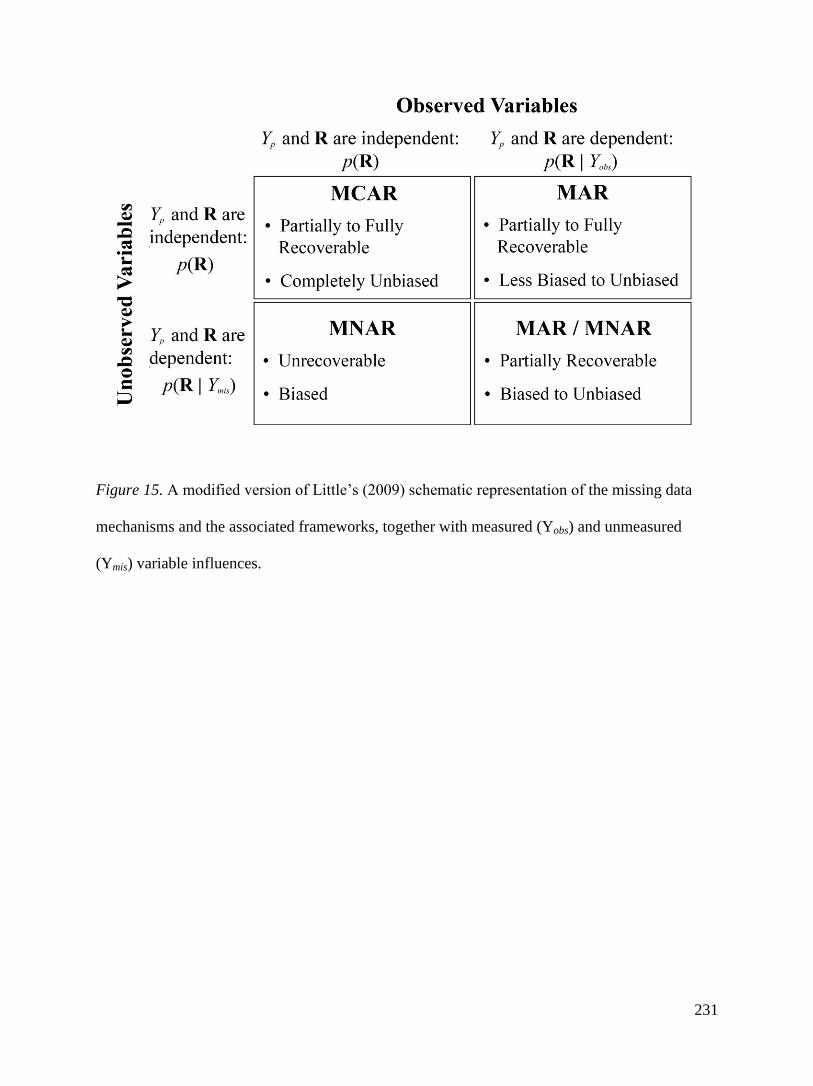
231

Figure 15. A modified version of Little’s (2009) schematic representation of the missing data

mechanisms and the associated frameworks, together with measured (Yobs) and unmeasured

(Ymis) variable influences.

232

Figure 16. A graphical representation of the MCAR missing data mechanism. Panel A provides a

conceptual diagram of MCAR where missingness (denoted R) is regressed on a random process.

Panel B provides a more detailed representation of MCAR that depicts p observed variables (Y1

– Yp) as boxes that are related (correlated) to some degree represented by solid reciprocal paths

where r ≠ 0. Additionally, there is no relationship between R and Y1 – Yp which is represented

by dotted reciprocal paths where r = 0. Visually, imagine that information can flow within the

diagram in Panel B through pathways are r ≠ 0. Note that the dot on the tip of the arrow point in

Panel A indicates a random process.

233

Figure 17. Univariate missing data pattern with missing on Y2 but not on Y1.

234

Figure 18. Diagram of the MAR missing data mechanism. Panel A offers a conceptual diagram

MAR that shows observed variables (Yobs) predicting the missing data (R). Panel B shows the

MAR mechanism in relation to p variables where Y2 contains missing data. Visually, imagine

that information can flow within the diagram in Panel B through pathways are r ≠ 0.

235

Figure 19. Diagram of the MNAR missing data mechanism. Panel A of Figure 21 provides a

theoretical explanation of MNAR. Here unmeasured variables (denoted Ymis) predict (i.e,. cause)

missingness. Panel B of Figure 21 shows the MNAR mechanism in relation to p variables where

Y2 contains missing data.

236

Figure 20. Diagram illustrating a conceptual overview of the missing data mechanisms where

each contributes to the observed missing data in a given study adopted from Little (2002).

237

Figure 21. Diagram illustrating the relationship between MNAR and MAR as a continuum

adopted from Graham (2012).

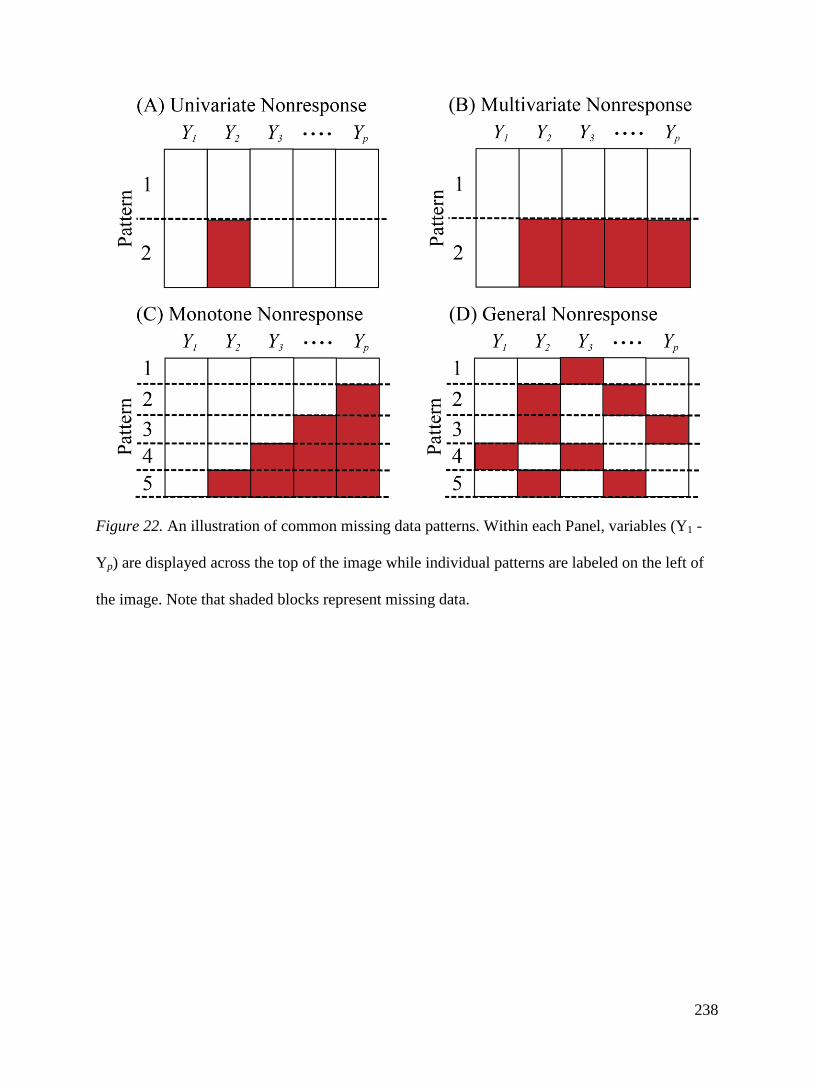
238

Figure 22. An illustration of common missing data patterns. Within each Panel, variables (Y1 -

Yp) are displayed across the top of the image while individual patterns are labeled on the left of

the image. Note that shaded blocks represent missing data.

239

Figure 23. A graphical demonstration of the Bayesian approach used by Rubin (1977) to address

missing data. Note that the multiplication of the prior distribution by the likelihood function

generates the posterior distribution. In this image the relative shapes of each distribution provide

information about how informative they are. That is, the height and width of each distribution

reflects the probability density for that distribution. For instance, the prior distribution in this

example is not very informative as it is relatively flat. An uninformative prior distribution could

be represented as a uniform distribution.

240

Figure 24. A graphical depiction of Rubin’s (1978a) multiple imputation procedure modified

from his original paper. Here each missing data point (shown as the start point of an arrow) is

replaced by a vector (denoted ,…,) of plausible values.

241

Figure 25. An illustration of Rubin’s (1987) multiple imputation procedure modified from

Enders (2010). The circle labeled “Missing Data” denotes a data set with incomplete data. The

arrows pointing from the “Missing Data” circle to the circles labeled “m = 1” through “m = k”

represent each imputation (as demonstrated in Figure 25). The arrows pointing from each m

imputation to the circles labeled “θ1” through “θk” illustrate a separate analysis of each imputed

data set, where the kth

θ represents a parameter estimate based on data from a particular

imputation. Finally, the arrows pointing from each of the kth

θ circles to the circle labeled

“Pooled Result” represent an process of combining (i.e., pooling) each of the imputed results.

The circle labeled “Pooled Result” represents the analytic solution informed by the MI process.

242

21.15 21.1421.15

20.2220.40

20.40 20.8119.96

19.96 20.69 17.21

17.21 19.5919.29

19.29 18.3316.91

16.91 15.4018.06

18.06 20.34

miss

obs

Y

Y X Y

21.14

20.81

20.69

19.59

18.33

15.40

20.34

obs

X

Figure 26. The Y and X vectors from the previous Yates method example. Notice that Yobs, Xobs

contain only associated values that are observed. That is, Yobs does not contain missing values

and Xobs does not contain the value 20.22 as it is associated with the Ymiss value.

243

Figure 27. Trace plot for the simulated mean of Y. The Y-axis contains a range of mean estimates

for Y and the X-axis displays the number of data augmentation cycles. This image demonstrates

iterative variation associated with each imputation. Notice that at the 10th

iteration (i.e., data

augmentation cycle) the Y parameter was 19.5 and at the 30th

iteration was 20.2, which are close

to the estimates derived above (e.g., 19.065 and 19.413). Also observe that an arbitrarily small

number of iterations were chosen (i.e., max P-step = 50) for clarity of presentation.

244

Figure 28. Illustration of a bivariate regression in the context of MI. Note that the superscript in

parentheses indicates the imputation number associated with each of the m beta weights.

245

Figure 29. Illustration of a missing data pattern with missing on Y but not on X.

246

Figure 30. A path diagram illustrating the range of population correlations (ρ) relative to the

analysis variables and the associated auxiliary variables.

247

Figure 31. A plot of simulation results showing bias associated with the exclusion of a cause or

correlate of missingness. Note that “AUXILIARY VARIABLE CORRELATION” denotes the

population correlation between Y and the omitted auxiliary variable (AUX1) and “XY

CORRELATION” refers to the population association among the variables X and Y (ρXY = .30).

248

Figure 32. Simulation results showing the bias reduction associated with including auxiliary

variables in a MNAR situation. Note that “AUXILIARY VARIABLE CORRELATION”

denotes the population correlation between Y and the omitted auxiliary variable (AUX1) and “XY

CORRELATION” refers to the population association among the variables X and Y (ρXY = .30).

249

Figure 33. Simulation results showing the relative power associated with including auxiliary

variables in a MCAR Situation. Note that “AUXILIARY VARIABLE CORRELATION”

denotes the population correlation between Y and the omitted auxiliary variable (AUX1) and

“RELATIVE POWER” refers to the estimated increase in power relative to a model with no

auxiliary variables.

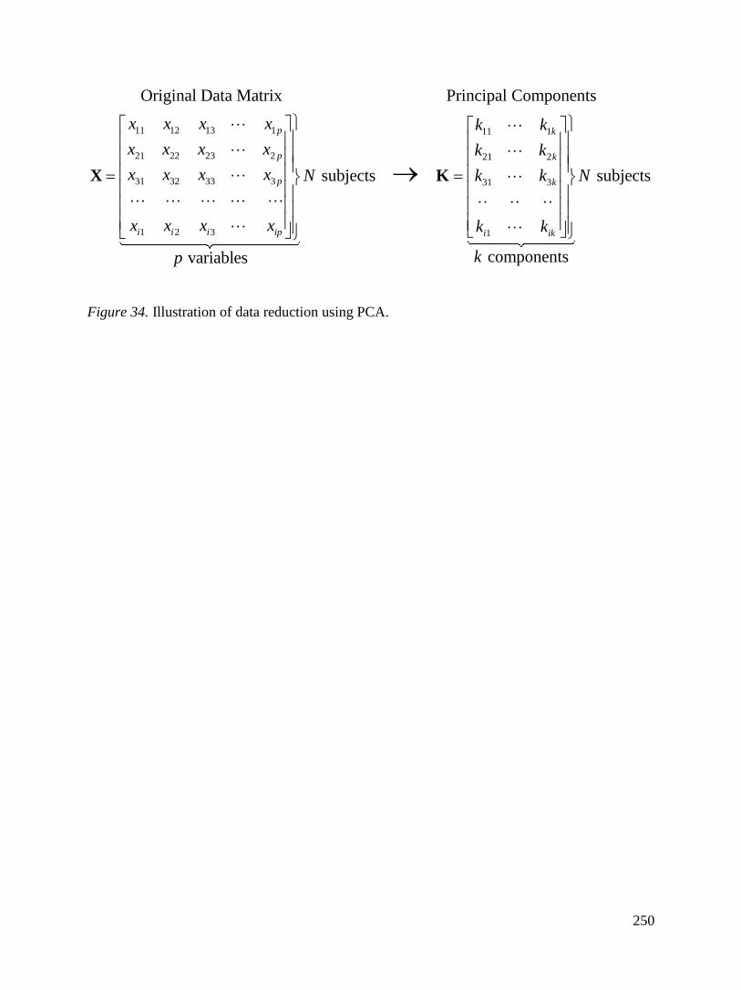
250

11 12 13 1

21 22 23 2

31 32 33 3

1 2 3

Original Data Matrix Principal Components

v

p

p

p

i i i ip

x x x x

x x x x

x x x x

x x x x

p

X

11 1

21 2

31 3

1

subjects subjects

componentsariables

k

k

k

i ik

k k

k k

N k k N

k k

k

K

Figure 34. Illustration of data reduction using PCA.

251

Figure 35. Scatterplot of the data in Table 10 (N = 25) with a correlation ellipse and regression

lines (see dotted lines) that reflect the arbitrary division between y regressed on x (where

0 1i i iY X e ) and of x regressed on y (where 0 1i i iX Y e ). Note 1 , the

unstandardized regression coefficient, represents the average change in Y for each unit change in

X or vice versa. Likewise, the error term ie represents the error associated with the prediction of

Y from X or vice versa (see Hays, 1994). The “Line of Best Fit” (which is the first principal

component) minimizes the sum of squared errors from each point irrespective of the

252

specification of a dependent and independent variable. The “Line of Worst Fit” (which is the

second principal component) minimizes the sum of squared errors not already explained by the

“Line of Best Fit”. In terms of the correlation ellipse, the “Line of Best Fit” corresponds to the

most expanded portion of the ellipse. Similarly, the “Line of Worst Fir” maps onto the most

compressed portion of the ellipse.

253

Figure 36. Illustration of the rotated scatterplot from Figure 37. Note that the “Line of Best Fit”

and “Line of Worst Fit” now occupy the original coordinate position of variables x and y.

Through principal axis rotation the locations of the new axes define the new variables (i.e., the

principal components). Note that the new variable called “Principal component 1”, explains most

of the variability in the scatterplot. Principal component 2 captures the remaining variance.

254

Fig

ure

37.

Illu

stra

tion o

f dat

a tr

ansf

orm

atio

n p

roce

ss f

rom

the

ori

gin

al d

ata m

atri

x t

o a

covar

iance

/corr

elat

ion m

atri

x a

nd t

hen

to

a se

t of

new

var

iable

s ca

lled

pri

nci

pal

com

ponen

ts.

255

Figure 38. Illustration of vector 1u as a trajectory in 2 dimensional space.

256

Figure 39. Illustration of scalar multiplication of vector 1u that results in vector 1.1u , a change in

the length of vector 1u .

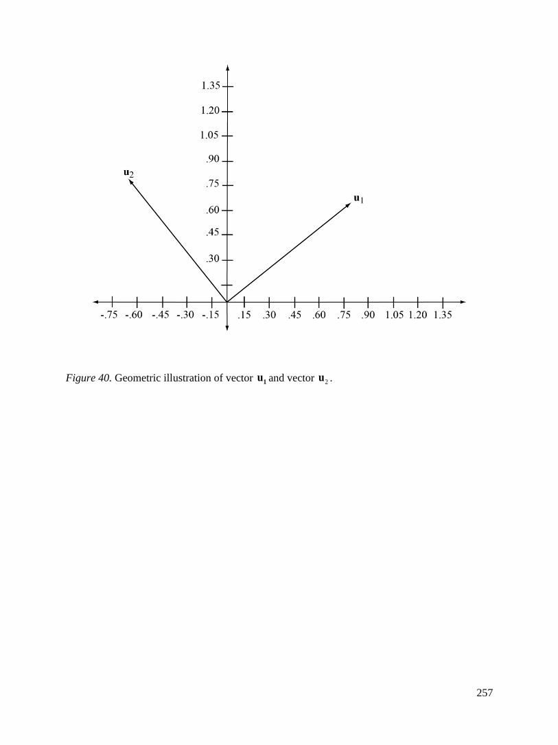
257

Figure 40. Geometric illustration of vector 1u and vector 2u .

258

Figure 41. Geometric illustration of the angle formed between the perpendicular vector 1u and

vector 2u .

259

Figure 42. Geometric representation of the angles of the rotated axes relative to the original

scatter plot’s x y coordinate positions. The fitted “Line of Best Fit” represents the first principal

component of the 2x2 covariance matrix S from the data in Table 10.

260

Figure 43. Geometric representation of the angles of the rotated axes relative to the original

scatter plot’s x y coordinate positions. The fitted “Line of Worst Fit” represents the second

principal component of the 2x2 covariance matrix S from the data in Table 10.

261

11 1

21 2

31 3

1

Principal Components

components

k

k

k

i ik

k k

k k

k k scores

k k

k

Figure 44. Illustration of k principal components as new variables that consist of i scores.

262

Figure 45. A graphical depiction of a likelihood function to depict convergence failure. Panel A

illustrates a typical unimodal likelihood function with one likely solution denoted as A. Panel B

shows a trimodal likelihood function with three possible likelihood solutions denoted A, B, and

C which correspond to different MLE of the mean.

263

Fig

ure

34. A

gra

phic

al

dep

icti

on o

f th

e data

augm

enta

tion c

onve

rgen

ce r

ate

s. P

anel

A w

as

sim

ula

ted b

ase

d o

n a

MA

R

mec

hanis

m t

o i

llust

rate

a s

yste

m w

ith s

om

e in

stab

ilit

y (d

enote

d b

y la

rge

syst

emati

c tr

ends

rela

tive

to

those

in P

anel

B).

In c

ontr

ast

, P

anel

B c

onta

ins

more

sta

ble

tre

nds

resu

ltin

g f

rom

MC

AR

sim

ula

ted d

ata

. N

ote

that

the

dash

ed r

efer

ence

line

repre

sents

the

true

popula

tion v

alu

e (i

.e., ρ

XY =

.30

).

Fig

ure

46.

A g

raphic

al d

epic

tion o

f th

e dat

a au

gm

enta

tion s

tabil

ity.

Let

the

das

hed

lin

e re

pre

sent

a re

fere

nce

lin

e fo

r th

e pop

ula

tion

val

ue

Pan

el A

(si

mula

ted

MA

R d

ata)

rep

rese

nts

rel

ativ

ely m

ore

inst

abil

ity t

han

Pan

el B

(si

mula

ted M

CA

R d

ata)

. M

ore

spec

ific

ally

,

note

that

the

esti

mat

ed d

ata

in P

anel

A c

onta

ins

larg

er s

yst

emat

ic d

ow

nw

ard

and u

pw

ard t

rends

rela

tive

to t

he

esti

mat

ed d

ata

in

Pan

el B

.

264

Figure 47. Exemplar general missing data pattern with missing on all variables except X.

265

Fig

ure

48.

Illu

stra

tion o

f th

e popula

tion m

odel

for

the

thre

e hom

ogen

eity

co

ndit

ions.

Pan

el A

rep

rese

nts

a p

opula

tion m

odel

wit

h a

unif

orm

corr

elat

ion o

f ρ =

.30 a

mon

g t

he

aux

ilia

ry v

aria

ble

s. P

anel

B s

how

s a

hig

h h

om

ogen

eity

condit

ion w

ith

corr

elat

ion m

agnit

udes

div

ided

into

fourt

hs

wit

h ρ

= .

20, .2

5, .3

5, an

d .

40.

Pan

el C

dem

on

stra

tes

the

low

ho

mo

gen

eity

condit

ion w

ith c

orr

elat

ion m

agnit

udes

div

ided

into

fourt

hs

wit

h ρ

= .10, .2

0, .4

0, an

d .50.

266

Figure 49. Illustration of the missing data patterns investigated across X, Y and p auxiliary

variables (note that some conditions include squared and cubed terms) where missingness is

shown as shaded areas. Panel A displays a univariate missing data pattern with missingness only

on Y (thus only two patterns of observed or missing data). Panel B shows a general missing data

pattern with missingness scattered throughout the data in a seemingly random fashion (with k

missing data patterns).

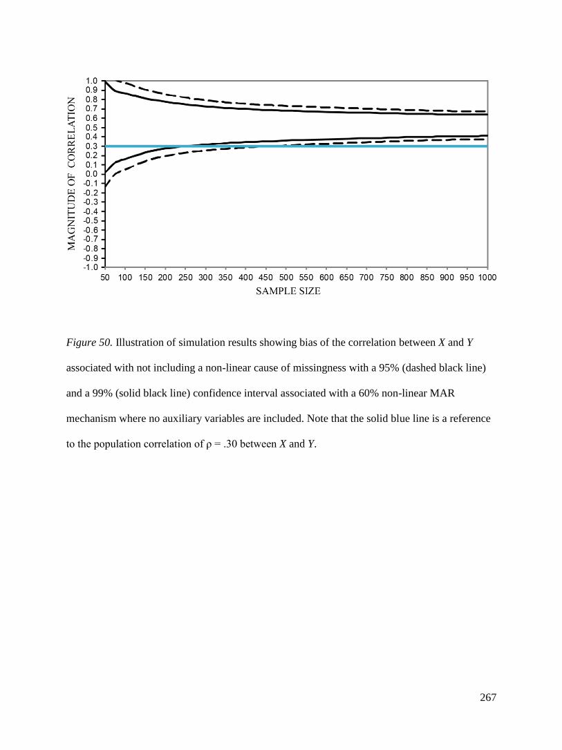
267

Figure 50. Illustration of simulation results showing bias of the correlation between X and Y

associated with not including a non-linear cause of missingness with a 95% (dashed black line)

and a 99% (solid black line) confidence interval associated with a 60% non-linear MAR

mechanism where no auxiliary variables are included. Note that the solid blue line is a reference

to the population correlation of ρ = .30 between X and Y.

268

Figure 51. Illustration of simulation results showing the correlation between X and Y where the

linear components (i.e., AUX1 and AUX2) of the interaction term (i.e., AUX1*AUX2) that caused

missingness are included with a 95% (dashed black line) and a 99% (solid black line) confidence

interval associated with a 60% non-linear MAR mechanism where all linear auxiliary variables

are included. Note that the solid blue line is a reference to the population correlation of ρ = .30

between X and Y.

269

Figure 52. Illustration of simulation results showing the correlation between X and Y where the

PCAAUX method is used with a 95% (dashed black line) and a 99% (solid black line) confidence

interval associated with a 60% non-linear MAR mechanism where a PCA auxiliary variable

which contains nonlinear information is included. Note that the solid blue line is a reference to

the population correlation of ρ = .30 between X and Y.

270

A raw data with missingness B rows with complete data only

21.15 21.14

20.22

20.40 20.81

19.96 20.69

17.21 19.59

19.29 18.33

16.91 15.40

18.06 20.34

missY

Y X

21.15 21.14

20.40 20.81

19.96 20.69

17.21 19.59

19.29 18.33

16.91 15.40

18.06 20.34

obs obs

Y X

Figure 53. The Y and X vectors for the Yates method example. Panel A demonstrates the raw

data with a missing values denoted Ymiss. Panel B contains only associated values (i.e., rows) that

are observed. That is, Yobs does not contain Ymiss and Xobs does not contain the value 20.22 as it

is in the same row (from the same case) as Ymiss.

271

Figure 54. A graphical depiction of joint events in a sample space (left). Panel A illustrates a

table of probabilities associated with independent joint events. Panel B demonstrates a table of

probabilities associated with non-independent joint events. This image shows the relationship

between the missing data probability distribution R, and the associated data probability

distribution Y.

272

Figure 55. Mean plots of the ECI key skills from the empirical data example. Panel A

demonstrates the key skills means across 3 – month intervals based on multiple imputation via

the AUX method. Panel B contains the key skills means across 3 – month intervals based on

multiple imputation via the PCAaux method. Note that GES_MEAN = the mean of gestures,

273

VOC_MEAN = the mean of vocalizations, WRD_MEAN = the mean of words, MUL_MEAN =

the mean of multiple words.

using principal component analysis (pca) to obtain

Documents