neural networks: principal component analysis (pca)
TRANSCRIPT

CHAPTERS 8
UNSUPERVISED LEARNING:
PRINCIPAL -COMPONENTS ANALYSIS (PCA)
CSC445: Neural Networks
Prof. Dr. Mostafa Gadal-Haqq M. Mostafa
Computer Science Department
Faculty of Computer & Information Sciences
AIN SHAMS UNIVERSITY
Credits: Some Slides are taken from presentations on PCA by :
1. Barnabás Póczos University of Alberta
2. Jieping Ye, http://www.public.asu.edu/~jye02
ASU-CSC445: Neural Networks
Prof. Dr. Mostafa Gadal-Haqq
Introduction
Tasks of Unsupervised Learning
What is Data Reduction?
Why we need to Reduce Data Dimensionality?
Clustering and Data Reduction
The PCA Computation
Computer Experiment
2
Outlines
ASU-CSC445: Neural Networks
Prof. Dr. Mostafa Gadal-Haqq 3
Unsupervised Learning
In unsupervised learning, the requirement is to discover significant patterns, or features, of the input data through the use of unlabeled examples.
That it, the network operates according to the rule:
“Learn from examples without a teacher”
ASU-CSC445: Neural Networks
Prof. Dr. Mostafa Gadal-Haqq
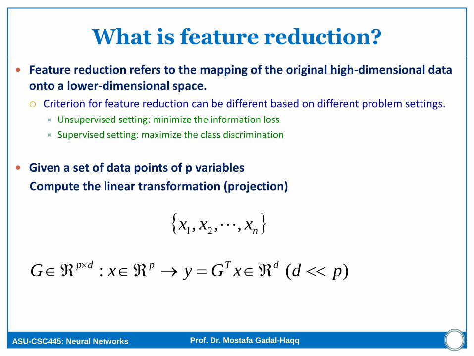
What is feature reduction?
Feature reduction refers to the mapping of the original high-dimensional data onto a lower-dimensional space.
Criterion for feature reduction can be different based on different problem settings.
Unsupervised setting: minimize the information loss
Supervised setting: maximize the class discrimination
Given a set of data points of p variables
Compute the linear transformation (projection)
nxxx ,,, 21
)(: pdxGyxG dTpdp

High Dimensional Data
Gene expression Face images Handwritten digits
Why feature reduction?
Most machine learning and data mining techniques may not be effective for high-dimensional data
Curse of Dimensionality
Query accuracy and efficiency degrade rapidly as the dimension increases.
The intrinsic dimension may be small.
For example, the number of genes responsible for a certain type of disease may be small.

Why feature reduction?
Visualization: projection of high-dimensional data onto 2D or 3D.
Data compression: efficient storage and retrieval.
Noise removal: positive effect on query accuracy.
What is Principal Component Analysis?
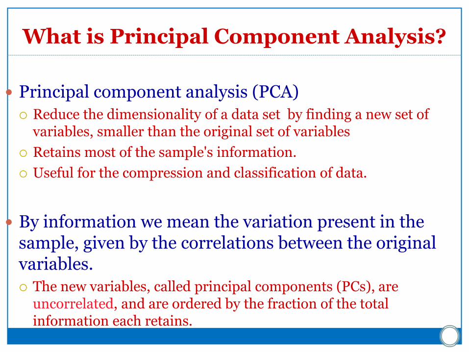
Principal component analysis (PCA)
Reduce the dimensionality of a data set by finding a new set of variables, smaller than the original set of variables
Retains most of the sample's information.
Useful for the compression and classification of data.
By information we mean the variation present in the sample, given by the correlations between the original variables.
The new variables, called principal components (PCs), are uncorrelated, and are ordered by the fraction of the total information each retains.

ASU-CSC445: Neural Networks
Prof. Dr. Mostafa Gadal-Haqq
principal components (PCs)
2z
1z
1z• the 1st PC is a minimum distance fit to a line in X space
• the 2nd PC is a minimum distance fit to a line in the plane
perpendicular to the 1st PC
PCs are a series of linear least squares fits to a sample,
each orthogonal to all the previous.

ASU-CSC445: Neural Networks
Prof. Dr. Mostafa Gadal-Haqq
Algebraic definition of PCs
.,,2,1,1
111 njxaxazp
i
ijij
T
p
nxxx ,,, 21
]var[ 1z
),,,(
),,,(
21
121111
pjjjj
p
xxxx
aaaa
Given a sample of n observations on a vector of p variables
define the first principal component of the sample
by the linear transformation
where the vector
is chosen such that is maximum.

ASU-CSC445: Neural Networks
Prof. Dr. Mostafa Gadal-Haqq
To find first note that
where
is the covariance matrix.
Algebraic Derivation of the PCA
Ti
n
i
i xxxxn
1
1
1a
11
1
11
1
2
11
2
111
1
1))((]var[
aaaxxxxan
xaxan
zzEz
Tn
i
T
ii
T
n
i
T
i
T
mean. theis 1
1
n
i
ixn
x
In the following, we assume the Data is centered.
0x
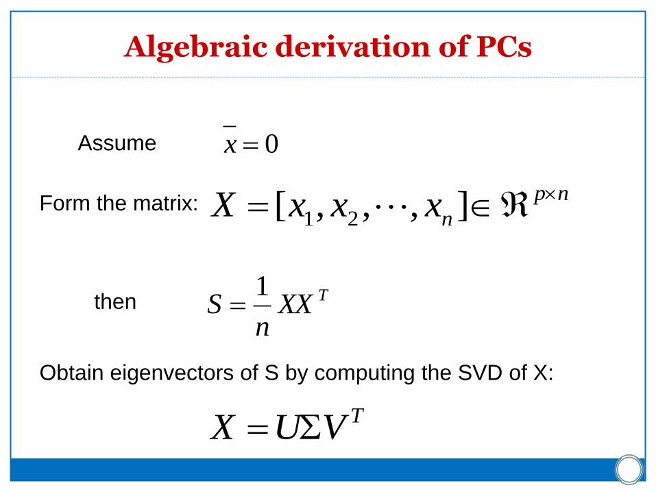
Algebraic derivation of PCs
np
nxxxX ],,,[ 21
0x
TXXn
S1
Assume
Form the matrix:
then
TVUX
Obtain eigenvectors of S by computing the SVD of X:

Principle Component Analysis
Orthogonal projection of data onto lower-dimension linear space that... maximizes variance of projected data (purple line)
minimizes mean squared distance between
data point and
projections (sum of blue lines)
PCA:

Principle Components Analysis
Idea:
Given data points in a d-dimensional space, project into lower dimensional space while preserving as much information as possible
Eg, find best planar approximation to 3D data
Eg, find best 12-D approximation to 104-D data
In particular, choose projection that minimizes squared error in reconstructing original data

Vectors originating from the center of mass
Principal component #1 points in the direction of the largest variance.
Each subsequent principal component…
is orthogonal to the previous ones, and
points in the directions of the largest variance of the residual subspace
The Principal Components
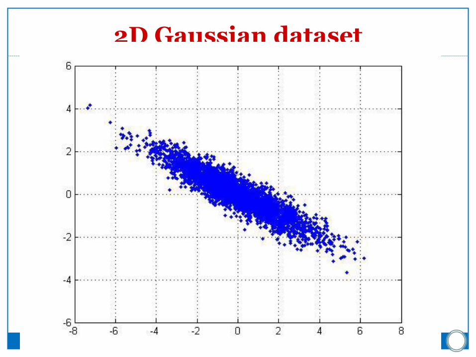
2D Gaussian dataset

1st PCA axis

2nd PCA axis

PCA algorithm I (sequential)
m
i
k
j
i
T
jji
T
km 1
21
11
})]({[1
maxarg xwwxwww
}){(1
maxarg1
2
i1
1
m
i
T
mxww
w
We maximize the
variance of the projection
in the residual subspace
We maximize the variance of projection of x
x’ PCA reconstruction
Given the centered data {x1, …, xm}, compute the principal vectors:
1st PCA vector
kth PCA vector
w1(w1Tx)
w2(w2Tx)
x
w1
w2 x’=w1(w1
Tx)+w2(w2Tx)
w

PCA algorithm II (sample covariance matrix)
Given data {x1, …, xm}, compute covariance matrix
PCA basis vectors = the eigenvectors of
Larger eigenvalue more important eigenvectors
m
i
T
im 1
))((1
xxxx
m
i
im 1
1xxwhere

PCA algorithm II PCA algorithm(X, k): top k eigenvalues/eigenvectors
% X = N m data matrix,
% … each data point xi = column vector, i=1..m
•
• X subtract mean x from each column vector xi in X
• X XT … covariance matrix of X
• { i, ui }i=1..N = eigenvectors/eigenvalues of
... 1 2 … N
• Return { i, ui }i=1..k % top k principle components
m
im 1
1ixx
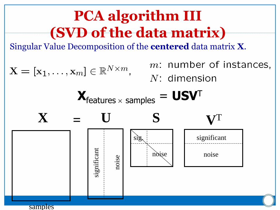
PCA algorithm III (SVD of the data matrix)
Singular Value Decomposition of the centered data matrix X.
Xfeatures samples = USVT
X VT S U =
samples
significant
noise
nois
e noise
signif
ican
t
sig.

PCA algorithm III Columns of U
the principal vectors, { u(1), …, u(k) }
orthogonal and has unit norm – so UTU = I
Can reconstruct the data using linear combinations of { u(1), …, u(k) }
Matrix S
Diagonal
Shows importance of each eigenvector
Columns of VT
The coefficients for reconstructing the samples

Face recognition
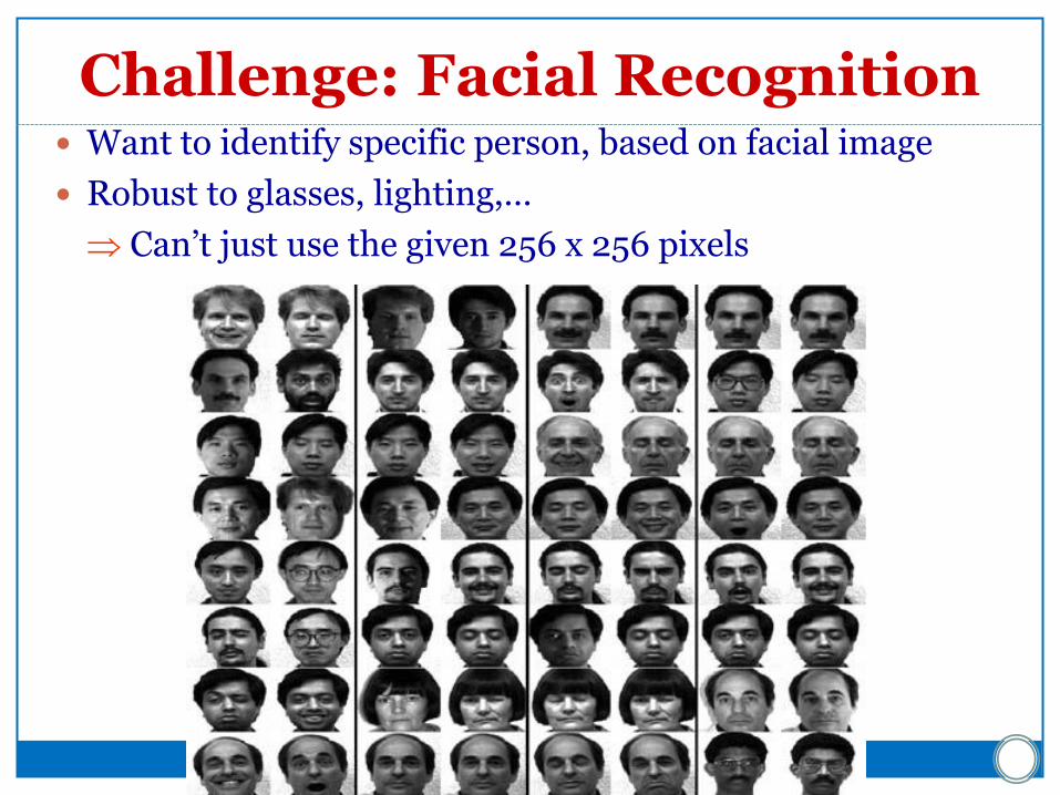
Challenge: Facial Recognition Want to identify specific person, based on facial image
Robust to glasses, lighting,…
Can’t just use the given 256 x 256 pixels

Applying PCA: Eigenfaces
Example data set: Images of faces
Famous Eigenface approach [Turk & Pentland], [Sirovich & Kirby]
Each face x is …
256 256 values (luminance at location)
x in 256256 (view as 64K dim vector)
Form X = [ x1 , …, xm ] centered data mtx
Compute = XXT
Problem: is 64K 64K … HUGE!!! 256 x
256
real va
lues
m faces
X =
x1, …, xm
Method A: Build a PCA subspace for each person and check which subspace can reconstruct the test image the best
Method B: Build one PCA database for the whole dataset and then classify based on the weights.

Computational Complexity
Suppose m instances, each of size N
Eigenfaces: m=500 faces, each of size N=64K
Given NN covariance matrix , can compute all N eigenvectors/eigenvalues in O(N3)
first k eigenvectors/eigenvalues in O(k N2)
But if N=64K, EXPENSIVE!

A Clever Workaround
Note that m<<64K Use L=XTX instead of =XXT
If v is eigenvector of L
then Xv is eigenvector of
Proof: L v = v
XTX v = v
X (XTX v) = X( v) = Xv
(XXT)X v = (Xv)
Xv) = (Xv)
256 x
256
real va
lues
m faces
X =
x1, …, xm

Principle Components (Method B)

Reconstructing… (Method B)
… faster if train with…
only people w/out glasses
same lighting conditions

Shortcomings Requires carefully controlled data:
All faces centered in frame
Same size
Some sensitivity to angle
Alternative:
“Learn” one set of PCA vectors for each angle
Use the one with lowest error
Method is completely knowledge free
(sometimes this is good!)
Doesn’t know that faces are wrapped around 3D objects (heads)
Makes no effort to preserve class distinctions

Facial expression recognition

Happiness subspace (method A)

Disgust subspace (method A)

Facial Expression Recognition Movies (method A)

Facial Expression Recognition Movies (method A)
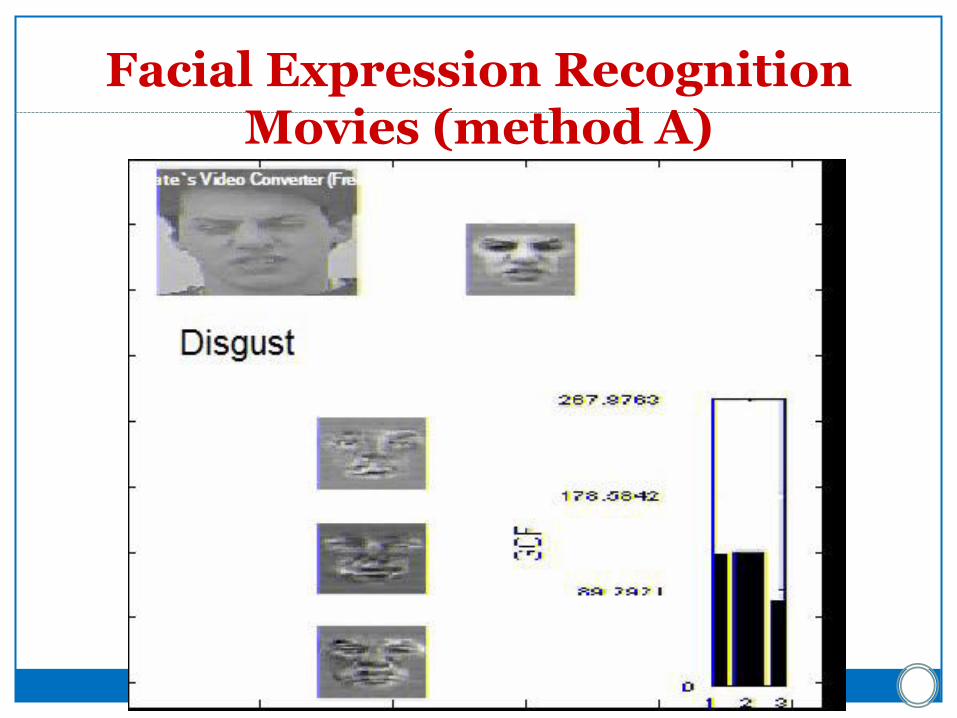
Facial Expression Recognition Movies (method A)
Image Compression

Original Image
• Divide the original 372x492 image into patches: • Each patch is an instance that contains 12x12 pixels on a grid
• View each as a 144-D vector

L2 error and PCA dim

PCA compression: 144D ) 60D

PCA compression: 144D ) 16D
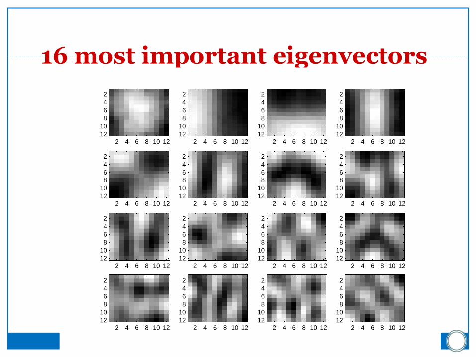
16 most important eigenvectors
2 4 6 8 10 12
2
4
6
8
10
122 4 6 8 10 12
2
4
6
8
10
122 4 6 8 10 12
2
4
6
8
10
122 4 6 8 10 12
2
4
6
8
10
12
2 4 6 8 10 12
2
4
6
8
10
122 4 6 8 10 12
2
4
6
8
10
122 4 6 8 10 12
2
4
6
8
10
122 4 6 8 10 12
2
4
6
8
10
12
2 4 6 8 10 12
2
4
6
8
10
122 4 6 8 10 12
2
4
6
8
10
122 4 6 8 10 12
2
4
6
8
10
122 4 6 8 10 12
2
4
6
8
10
12
2 4 6 8 10 12
2
4
6
8
10
122 4 6 8 10 12
2
4
6
8
10
122 4 6 8 10 12
2
4
6
8
10
122 4 6 8 10 12
2
4
6
8
10
12
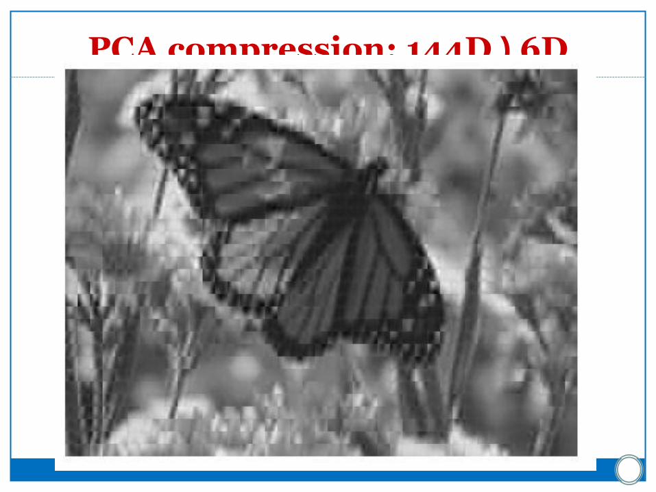
PCA compression: 144D ) 6D

2 4 6 8 10 12
2
4
6
8
10
12
2 4 6 8 10 12
2
4
6
8
10
12
2 4 6 8 10 12
2
4
6
8
10
12
2 4 6 8 10 12
2
4
6
8
10
12
2 4 6 8 10 12
2
4
6
8
10
12
2 4 6 8 10 12
2
4
6
8
10
12
6 most important eigenvectors

2 4 6 8 10 12
2
4
6
8
10
12
2 4 6 8 10 12
2
4
6
8
10
12
2 4 6 8 10 12
2
4
6
8
10
12
3 most important eigenvectors

PCA compression: 144D ) 3D

2 4 6 8 10 12
2
4
6
8
10
12
2 4 6 8 10 12
2
4
6
8
10
12
2 4 6 8 10 12
2
4
6
8
10
12
3 most important eigenvectors

PCA compression: 144D ) 1D

60 most important eigenvectors
Looks like the discrete cosine bases of JPG!...

2D Discrete Cosine Basis
http://en.wikipedia.org/wiki/Discrete_cosine_transform
Noise Filtering

Noise Filtering, Auto-Encoder…
x x’
U x
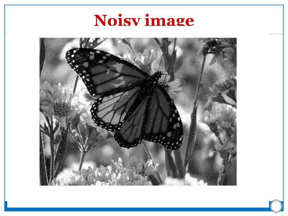
Noisy image
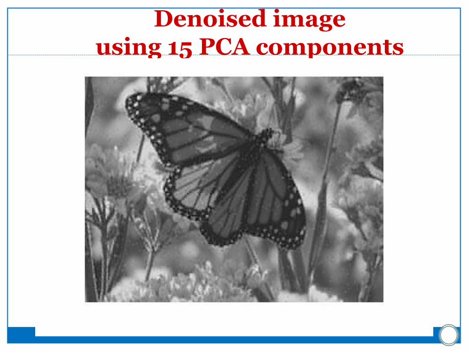
Denoised image using 15 PCA components

PCA Shortcomings

PCA, a Problematic Data Set
PCA doesn’t know labels!

PCA vs Fisher Linear Discriminant
PCA maximizes variance, independent of class
magenta
FLD attempts to separate classes
green line

PCA, a Problematic Data Set
PCA cannot capture NON-LINEAR structure!
PCA Conclusions
PCA finds orthonormal basis for data Sorts dimensions in order of “importance” Discard low significance dimensions
Uses: Get compact description Ignore noise Improve classification (hopefully)
Not magic: Doesn’t know class labels Can only capture linear variations
One of many tricks to reduce dimensionality!
Applications of PCA
Eigenfaces for recognition. Turk and Pentland. 1991.
Principal Component Analysis for clustering gene expression data. Yeung and Ruzzo. 2001.
Probabilistic Disease Classification of Expression-Dependent Proteomic Data from Mass Spectrometry of Human Serum. Lilien. 2003.

PCA for image compression
d=1 d=2 d=4 d=8
d=16 d=32 d=64 d=100 Original
Image