using neural networks to predict spatial structure in ecological systems

Ecological Modelling 179 (2004) 393–403

Using neural networks to predict spatial structurein ecological systems

M.J. Aitkenheada,∗, M.J. Mustardb, A.J.S. McDonaldca The Macaulay Institute, Craigiebuckler, Aberdeen AB15 8QH, Scotland, UK

b Royal Botanic Gardens Kew, Richmond TW9 3AE, Surrey, UKc Department of Plant and Soil Science, School of Biological Sciences, Cruickshank Building,

St Machar Drive, Aberdeen AB24 3UU, Scotland, UK

Received 15 July 2003; received in revised form 14 April 2004; accepted 3 May 2004

Abstract

We describe an approach in which a neural network (NN) can be trained on sets of driving variables (inputs) and outputvariables relating to spatial structure. The trained NN provides a predictive tool for defining spatial structure in a specifiedecological system. We demonstrate the approach using a modified version of the Crawley and May [J. Theor. Biol. 125 (1987)475] model that describes simplified annual/perennial plant interactions in a disturbed system. The model is implemented withina cellular automaton with randomised start conditions and is run for periods of up to 50 time steps (50 years). Neural networksare trained using a large set of modelled situations, and the ability of the network to predict plant spatial distributions is thenmeasured. Different image analysis methods are applied to the plant array, and the ability of each method to provide an accuratedescription of the end-state of the modelled system is investigated. Reconstruction of the plant array from these image analysismeasurements is carried out using a stochastic error minimisation method. The partial derivatives method is applied to the trainedneural network in order to determine which variables input to the model most strongly influence the eventual plant populationdistribution. In the example presented, it is found that a relatively simple boundary:area ratio measurement provides a rapid andeffective method of describing the spatial structure of the plant community, while the variables that are most influential on thesystem’s end-state are those describing annual fecundity and perennial mortality rates.© 2004 Elsevier B.V. All rights reserved.

Keywords: Crawley–May; Cellular automata; Neural networks; Population dynamics; Community structure

1. Introduction

Ecological communities generally feature spatial,dynamic patterns. These are apparent from inspec-tion of real community images (e.g. spatial patternsof vegetation;Pachepsky et al., 2001; Wells et al.,

∗ Corresponding author. Tel.:+44-1224-498200.E-mail address: [email protected]

(M.J. Aitkenhead).

2001; Hartley and Amos, 1999) or the output of spa-tial array models (e.g. simulated vegetation structure).Watkinson et al. (2000)showed that interactions withperennials reduced annual seedling recruitment. Theystudied annual grass structures at three scales andargued that the characteristics of dynamics at largescales are explained by processes operating at smallscales (i.e. at regional scales the population is actuallya metapopulation, rather than a collection of uncon-nected local populations).Hui and Li (2003)andWei

0304-3800/$ – see front matter © 2004 Elsevier B.V. All rights reserved.doi:10.1016/j.ecolmodel.2004.05.008

394 M.J. Aitkenhead et al. / Ecological Modelling 179 (2004) 393–403

et al. (2003)showed that habitat destruction and dis-turbance have strong effects on metapopulation per-sistence and regulation.

The concept of a metapopulation is an important onein population dynamics.Freckleton and Watkinson(2002)reviewed the concept of a metapopulation andshowed that the concept of many smaller populationsexisting within small niches does not always hold, be-cause suitable niches of large spatial extent can ex-ist without being fully occupied by a population. Thisleads to the argument that a spatially heterogeneousmetapopulation can exist within an area of continuoussuitable conditions if there is something else gettingin its way (e.g. another species). Scale is an impor-tant consideration when dealing with population dy-namics, and is closely tied to the concept of spatialdistribution.

Although it is often instructive to simply visualise aseries of emergent spatial structures in real or virtualsystems, it is often more useful to measure propertiesof the system and to predict its future behaviour fromsome initial state. For example, in the case of real orvirtual plant communities, it would be useful to knowif one species or species grouping will eventually leadto the elimination of one or more other species or ifall species will reach some kind of stable populationbalance. It may also be informative to predict the spa-tial distribution of species and bare ground areas fromsome initial state. Will one or more species be scat-tered randomly, or will there be clumping? What sizewill the areas of bare ground be, and for how long willthey remain empty? These questions and others maybe answered through a combination of modelling andmorphological image analysis. There are many dif-ferent approaches to spatial analysis, some of whichmay be more relevant than others to the spatial anal-ysis of a particular system. For example,Guo et al.(2000)assessed the relevance of different approachesto analysing the relationship between abundance anddistribution of annual plants, in both spatial and tem-poral measures.

Successful modelling and analysis of spatial dy-namics in an ecological system requires quality in-formation for defining rules of individual behaviour(e.g. growth and reproduction) and rules of interactionbetween neighbouring individuals and their environ-ment. Even in a relatively simple ecological system(e.g. two or three functional types), there are still suf-

ficient numbers of variables used in defining individ-ual performance and rules of interaction to make theuse of many statistical analyses difficult or impossible.Here, we discuss an approach based on neural network(NN) theory as a means of determining non-linear re-lationships between descriptors of complex multivari-ate systems. NNs are capable of adjusting themselvesthrough error-reduction methods in order to mimic theinput–output variable mapping of complex systems. Afrequently voiced objection to using neural networkshas been that they constitute an inscrutable ‘black box’from which the learned relationships cannot be ob-tained. This is no longer a valid statement, as methodsexist which allow the black box to be opened and itscontents examined. For example,Gevrey et al. (2003)showed that the partial derivatives method, when ap-plied to backpropagation neural networks, gave a use-ful measure of the influence of each input variable onspecific output variables.

Austin (2002) argues that more attention shouldbe paid to ecological theory when developing statis-tical models of population dynamics, and that manymodelling assumptions are often oversimplificationsor are flawed. This is an assertion which, in the caseof modelling specific systems, is certainly valid. How-ever, in order to demonstrate the (generic) usefulnessof the NN approach, we require a model that is bothsimple enough to implement whilst providing somelevel of ecological realism. We consider a useful, il-lustrative example to be the seminal work byCrawleyand May (1987)that provides an individual-based ap-proach to modelling spatial interactions between an-nual and perennial plants. Their model captures someof the main features associated with mortality and re-cruitment of annuals and perennials although it alsofeatures much inadequacy of biological realism. Forexample, in the Crawley and May model, annual fe-cundity and perennial (clonal) spread do not featurea growth dependency. However, their model has thedistinct advantage of having a relatively small numberof clearly defined rules for individual behaviour, in-teractions between neighbours and spatial occupancy.Our approach has been to use a modified version ofthe Crawley and May model, featuring a disturbancevariable which impacts on the persistence of perenni-als and annuals and increases the available space forrecruitment. We carried out a large number of simula-tions that resulted in interesting, emergent spatial dy-

M.J. Aitkenhead et al. / Ecological Modelling 179 (2004) 393–403 395

namics, appropriate to illustrate the usefulness of theNN approach in predicting spatial structure.

The assumptions made in the model provide a goodmethod of demonstrating how it works (afterCrawleyand May (1987)):

1. Two plant species exist: an annual, which spreadsby seeds, and a perennial which spreads laterallyinto neighbouring cells.

2. The plants exist in a spatially uniform environ-ment. In the original model, this was a hexagonalpattern. We have adapted it to a regular pattern ofrows and columns.

3. Each cell accommodates a maximum of one plant.4. The time unit of the model represents one gener-

ation of the annual plant.5. In any one generation, the perennial is capable of

occupying only those empty cells immediately ad-jacent to it, and may occupy any number of these.

6. In competition for specific cells, perennials al-ways exclude the annuals.

7. The annual has no effect on the demography ofthe perennial.

8. In any generation, the order of events is as follows:(a) death of perennials; (b) birth of perennials; (c)recruitment of annuals from seed.

9. Recruitment of annuals by seed can only occur inempty cells.

10. The probability of recruitment by annuals in anyempty cell is a function of the number of seedsproduced in the previous generation. Specifically,this function is given as 1− e−s, wheres equalsthe number of seeds per cell, and the entire cropof annual seeds is distributed at random over allcells.

11. Death of perennials occurs in each generation withprobability independent of the age of the plant.

12. For each empty cell, the probability of being in-vaded by a perennial from a given neighbouringcell is given byb, and if k neighbours containperennials then the probability that the cell is in-vaded is equal to 1− (1 − b)k.

13. Disturbance here takes the form of squares of dif-ferent sizes and frequency within which all vege-tation is removed.

14. The array is wrapped to avoid edge effects, so thatthe left-hand and right-hand edges are connected,and the top and bottom edges are connected.

2. Methods

2.1. Plant array modelling

Eight variables are used to describe the properties ofthe simulated plant annual competition environment:initial annual count; initial perennial count; rate ofperennial spread; perennial mortality rate; annual fe-cundity; disturbance count per year; disturbance size;number of years (time steps) for which the simulationruns. The simulation is stopped at the end of this num-ber of steps and image analysis techniques are appliedto the array, giving a total of 26 measured variablesassociated with array structure.

The operation of the Crawley–May simulation isrelatively simple, and consists of the following proce-dures carried out repeatedly, once for every time step:

1. Kill off the existing annuals and a proportion of theperennials.

2. Seed annuals.3. Spread perennials.4. Create disturbances.

The predetermined control variables given aboveare used to determine which cells in the array becomeoccupied by annuals or perennials, or which ones areemptied by disturbances.

2.2. Image analysis

2.2.1. Boundary:area ratioFor each of the three cover types (annual, perennial

and bare ground), the total number of cells was mea-sured. The boundary between each cell and its eightneighbours was also determined, and a sum of eachof the nine permutations made. In each case, the max-imum ratio of boundary length to area equals eighttimes the total count of the central cell type consid-ered, and so in order to have values in the range [0, 1],each of the nine boundary lengths was divided by thecorresponding cover count multiplied by eight. Val-ues closer to 0 indicate more clumped structures whilevalues closer to 1 indicate more randomly scatteredpopulations.

This method has similarities to several landscapemetrics commonly used in geography and landscapeecology, including landscape shape index, patch den-sity and edge density. Each of these measures has been


shown to have a linear response to scale change (Wuet al., 2002), making it relatively easy to apply themat multiple resolutions and landscape scales.

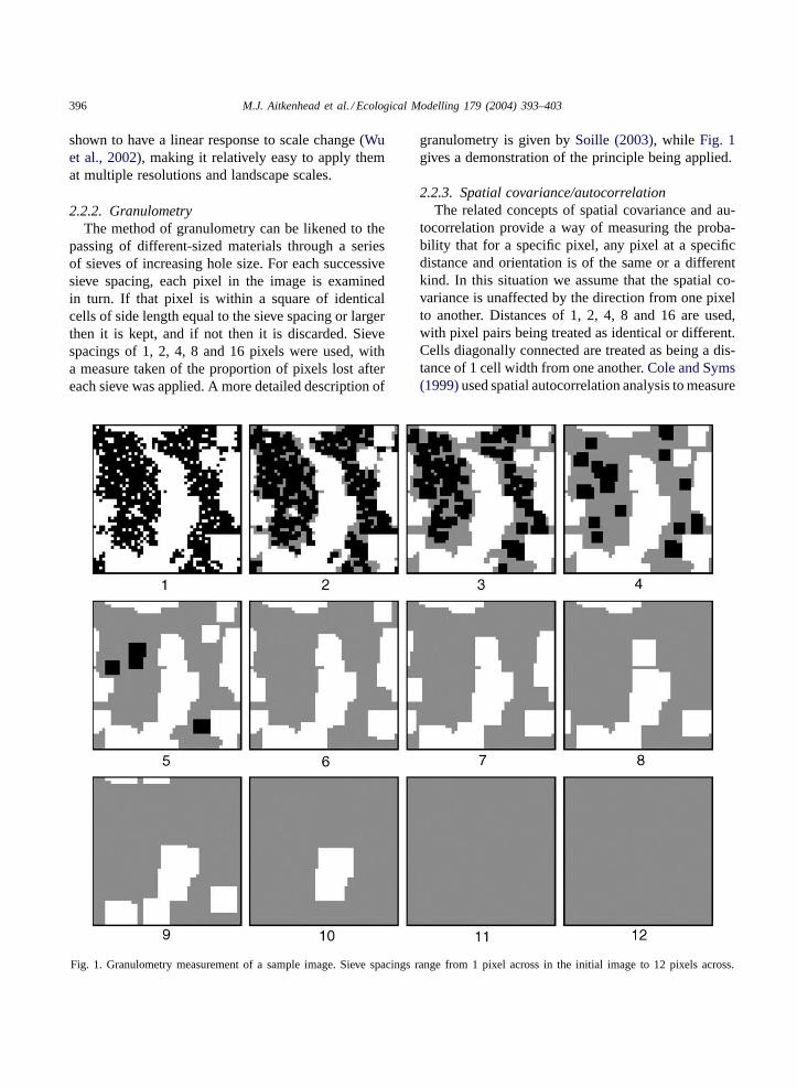
2.2.2. GranulometryThe method of granulometry can be likened to the

passing of different-sized materials through a seriesof sieves of increasing hole size. For each successivesieve spacing, each pixel in the image is examinedin turn. If that pixel is within a square of identicalcells of side length equal to the sieve spacing or largerthen it is kept, and if not then it is discarded. Sievespacings of 1, 2, 4, 8 and 16 pixels were used, witha measure taken of the proportion of pixels lost aftereach sieve was applied. A more detailed description of

Fig. 1. Granulometry measurement of a sample image. Sieve spacings range from 1 pixel across in the initial image to 12 pixels across.

granulometry is given bySoille (2003), while Fig. 1gives a demonstration of the principle being applied.

2.2.3. Spatial covariance/autocorrelationThe related concepts of spatial covariance and au-

tocorrelation provide a way of measuring the proba-bility that for a specific pixel, any pixel at a specificdistance and orientation is of the same or a differentkind. In this situation we assume that the spatial co-variance is unaffected by the direction from one pixelto another. Distances of 1, 2, 4, 8 and 16 are used,with pixel pairs being treated as identical or different.Cells diagonally connected are treated as being a dis-tance of 1 cell width from one another.Cole and Syms(1999)used spatial autocorrelation analysis to measure


the distribution of damage to kelp, whilePurves andLaw (2002)used spatial covariance functions for inter-and intraspecies correlation.Friedman et al. (2001)showed that autocorrelation patterns tended to be pos-itive for a species, while interspecific autocorrelationstended to be neutral or negative.Overmars et al. (2003)also describe methods of spatial autocorrelation mea-surement.

2.2.4. Power law size scalingIn many natural systems, a relationship exists be-

tween the size of a particular phenomena and the num-ber of occurrences of that phenomena. This relation-ship commonly takes the form of a power law, withthe frequency of occurrence (F) being proportional tothe magnitude (M) raised to some negative powerβ

(Eq. (1)).

F = αM−β (1)

Belyea and Lancaster (2002)examined dynamics ofpeat bog pools and used a power relationship betweenpool size and pool count. A similar method is usedhere, with the logarithm of the size of continuous areasof each species being plotted against the frequency ofoccurrence of areas of this size in the array. A best-fitline is drawn for each curve, the gradient of whichis the value of the power scaling factor. A maximumvalue of 10 is set for the power scaling factor, withvalues divided by 10 to normalise them onto the range[0, 1]. This scaling factor is determined for each ofthe three cover types in the array and a mean is takenof the three values.

2.2.5. Information fractal dimensionAlados et al. (2003)used fractal analyses as well as

autocorrelation measurements to quantify spatial dis-tributions of plants. Their fractal dimension measure-ment, the information fractal dimension (IFD), is cal-culated by finding the gradient of the line in a graphof log(1/E) (on thex-axis) againstP(E), whereE isthe one-dimensional transect length andP(E) is theprobability of finding that species along the transect.The value is restricted to the range [0, 1]. Lower val-ues indicate a more aggregated structure, while highervalues indicate more random distributions. A separatevalue of IFD is determined for each cover type.

2.3. Neural network training

The most commonly used neural network train-ing technique for mathematical modelling is that ofbackpropagation. While other methods have been usedfor pattern recognition and behavioural modification,the backpropagation method is superior at discoveringunknown mathematical relationships between systemvariables. The technique consists of an error-reducingmechanism and is described in, amongst other places,Rumelhart et al. (1986).

A separate network was constructed for each of the26 output variables (seeTable 1), with eight inputnodes, 100 nodes in a single hidden layer and a singleoutput node corresponding to the relevant variable.The network was trained using the results of 2000simulation runs, with a total of 10 000 training steps(each simulation used five times). Validation of thetrained NNs was carried out using 2000 runs that werenot used to train the networks.

2.4. Testing the approach: array reconstruction

The trained neural networks were used to providepredicted values for the test simulation run results,and these predicted values were used in array recon-struction. This process was carried out for 100 ofthe test data sets, with each of the five image anal-ysis measurement predictions used to reconstruct aplant array with corresponding measurements. In eachcase (boundary:area ratio, granulometry, autocorrela-tion, power law size scaling and information fractaldimension), the predicted proportion of the grid occu-pied by each cover type was used in addition to thefactors considered.

The actual method used for array construction wasa stochastic, error-reducing mechanism by which in-dividual cells in the initially randomised array (eachcell allocated one of the three states at random) wereflipped randomly between states (empty, annual andperennial), and the array re-measured using the rele-vant image analysis method. If the switch improvedthe error between the actual and desired measure-ments then it was kept, and if not it was abandoned.A small randomising element (a value of 0.01 was setafter trial and error) allowed a small proportion of thenon-improving switches to be kept, and so prevent thesystem being trapped in a local error minimum. The


Table 1Name and description of each of the output variables associated with spatial analysis of plant arrays

Variable name Variable description

Annuals (Aa) Proportion of array occupied by annualsPerennials (Ap) Proportion of array occupied by perennialsEmpty (Ae) Proportion of array occupied by empty cellsBaa Number of annual–annual boundaries as a proportion of maximum possibleBae Number of annual–empty boundaries as a proportion of maximum possibleBap Number of annual–perennial boundaries as a proportion of maximum possibleBpa Number of perennial–annual boundaries as a proportion of maximum possibleBpe Number of perennial–empty boundaries as a proportion of maximum possibleBpp Number of perennial–perennial boundaries as a proportion of maximum possibleBea Number of empty–annual boundaries as a proportion of maximum possibleBee Number of empty–empty boundaries as a proportion of maximum possibleBep Number of empty–perennial boundaries as a proportion of maximum possibleGranulometry1 Proportion of cells lost after passing through sieve spacing of 1Granulometry2 Proportion of cells lost after passing through sieve spacing of 2Granulometry4 Proportion of cells lost after passing through sieve spacing of 4Granulometry8 Proportion of cells lost after passing through sieve spacing of 8Granulometry16 Proportion of cells lost after passing through sieve spacing of 16Autocorrelation1 Spatial autocorrelation of cells at a distance of 1 cell widthAutocorrelation2 Spatial autocorrelation of cells at a distance of 2 cell widthsAutocorrelation4 Spatial autocorrelation of cells at a distance of 4 cell widthsAutocorrelation8 Spatial autocorrelation of cells at a distance of 8 cell widthsAutocorrelation16 Spatial autocorrelation of cells at a distance of 16 cell widthsPower law Relationship between size of cluster and number of clustersFractal dima Fractal dimension describing clustering of annualsFractal dimp Fractal dimension describing clustering of perennialsFractal dime Fractal dimension describing clustering of empty space

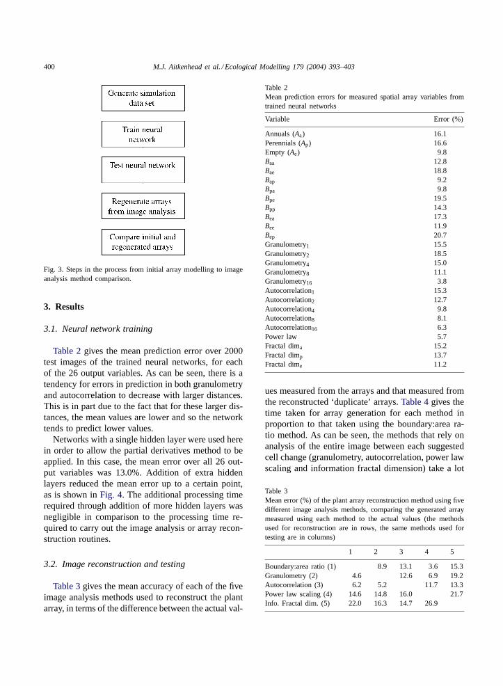
error reduction process halted when the error had beenreduced to 1% of its initial value upon randomisationof the array.Fig. 2 gives an example of the processover time as the system evolves from its initial randomstate towards specified values (Aa = 0.4,Ap = 0.4,Ae= 0.2,Baa= 0.8,Bap= 0.1,Bae= 0.1,Bpa = 0.1,Bpp= 0.6, Bpe = 0.3, Bea = 0.3, Bep = 0.3, Bee = 0.4).Fig. 3depicts the steps taken in going from the initialdata set obtained through array modelling and sub-sequent measurement, to the eventual comparison ofdifferent image analysis methods against one another.

2.5. Testing the approach: network analysis

The partial derivatives method allows us to tell therelative influence of each input variable on a particularoutput variable. The method obtains its name fromthe use of partial derivatives as a expression of howmuch one of many inputs has an affect on the outputvariables. As explained byGevrey et al. (2003), this

measure of influence is given by the sum of squaresdifference (SSD), which is given by

SSDi =N∑

j=1

(dij)2 (2)

dij = Sj

Nh∑

h=1

whoIhj(1 − Ihj)wih (3)

whereSj is the derivative of output neuronj with re-spect to activation,who is the weighting of synapsesconnecting the hidden layer and the output node,wihis the weighting of synapses connecting the input layerand the hidden layer, andIhj is the response of thehthhidden neuron. This method only applies to networkswith a single hidden layer, and to nodes that are ac-tivated using the sigmoid function. Higher values ofthe mean SSD correspond to input nodes whose ac-tivation is more influential upon the activation of theoutput nodes.


Fig. 2. The error-reducing array construction algorithm in action, showing the alteration to the array from initially random to havingboundary:area ratios of 0.75 for each cover type.


Fig. 3. Steps in the process from initial array modelling to imageanalysis method comparison.

3. Results

3.1. Neural network training

Table 2gives the mean prediction error over 2000test images of the trained neural networks, for eachof the 26 output variables. As can be seen, there is atendency for errors in prediction in both granulometryand autocorrelation to decrease with larger distances.This is in part due to the fact that for these larger dis-tances, the mean values are lower and so the networktends to predict lower values.

Networks with a single hidden layer were used herein order to allow the partial derivatives method to beapplied. In this case, the mean error over all 26 out-put variables was 13.0%. Addition of extra hiddenlayers reduced the mean error up to a certain point,as is shown inFig. 4. The additional processing timerequired through addition of more hidden layers wasnegligible in comparison to the processing time re-quired to carry out the image analysis or array recon-struction routines.

3.2. Image reconstruction and testing

Table 3gives the mean accuracy of each of the fiveimage analysis methods used to reconstruct the plantarray, in terms of the difference between the actual val-

Table 2Mean prediction errors for measured spatial array variables fromtrained neural networks

Variable Error (%)

Annuals (Aa) 16.1Perennials (Ap) 16.6Empty (Ae) 9.8Baa 12.8Bae 18.8Bap 9.2Bpa 9.8Bpe 19.5Bpp 14.3Bea 17.3Bee 11.9Bep 20.7Granulometry1 15.5Granulometry2 18.5Granulometry4 15.0Granulometry8 11.1Granulometry16 3.8Autocorrelation1 15.3Autocorrelation2 12.7Autocorrelation4 9.8Autocorrelation8 8.1Autocorrelation16 6.3Power law 5.7Fractal dima 15.2Fractal dimp 13.7Fractal dime 11.2

ues measured from the arrays and that measured fromthe reconstructed ‘duplicate’ arrays.Table 4gives thetime taken for array generation for each method inproportion to that taken using the boundary:area ra-tio method. As can be seen, the methods that rely onanalysis of the entire image between each suggestedcell change (granulometry, autocorrelation, power lawscaling and information fractal dimension) take a lot

Table 3Mean error (%) of the plant array reconstruction method using fivedifferent image analysis methods, comparing the generated arraymeasured using each method to the actual values (the methodsused for reconstruction are in rows, the same methods used fortesting are in columns)

1 2 3 4 5

Boundary:area ratio (1) 8.9 13.1 3.6 15.3Granulometry (2) 4.6 12.6 6.9 19.2Autocorrelation (3) 6.2 5.2 11.7 13.3Power law scaling (4) 14.6 14.8 16.0 21.7Info. Fractal dim. (5) 22.0 16.3 14.7 26.9


Fig. 4. Variation in the percentage error of the neural network prediction of image analysis factors with number of hidden layers, averagedover 100 runs of each network.

longer than the method which does not (boundary:arearatio).

3.3. Partial derivatives testing

It was found that the relative importance of eachinput variable, as measured with the partial derivativesmethod, varied with each output variable.Table 5givesthe number of times that each input node was foundto be most influential, whileTable 6gives the meanSSD value (as defined inSection 2.5) for each inputvariable, averaged over all output variables and 2000testing data sets.

Table 4Relative time taken to reconstruct plant array using each imageanalysis method

Method Relative time to generate array

Boundary:area ratio 1Granulometry 6.97Autocorrelation 4.45Power law scaling 17.34Info. fractal dim. 2.2

Table 5The number of times each input variable was found to be mostinfluential with respect to the 26 output variables

Input variable ‘Most influential’ frequency

Annuals sown 1Perennials sown 1Perennial growth rate 1Perennial mortality rate 12Annual fecundity 7Disturbance frequency 1Disturbance size 1Years simulated 2

4. Discussion

While visualisations of the array reconstructionmethods do not in themselves give us any additionalinformation (although they can prove instructive as towhat particular array types look like), the constructionof these arrays according to one image measurementtechnique and its subsequent analysis by other meth-ods can provide us with a useful way of determiningwhich morphological measurements have the mostmeaning as represented by their ability to generate


Table 6Mean SSD values calculated for each input variable, giving relativeimportance with respect to output variable activation in a trainedneural network

Input variable SSD Standard deviation

Annuals sown 0.0011 0.0014Perennials sown 0.0017 0.0021Perennial growth rate 0.0084 0.0114Perennial mortality rate 0.0221 0.0265Annual fecundity 0.0146 0.0200Disturbance frequency 0.0022 0.0024Disturbance size 0.0014 0.0017Years simulated 0.0025 0.0038

realistic arrays. In this case, realism is taken to meanthe accuracy as measured by several different imageanalysis methods. When determined in this way, it isshown that autocorrelation provides the best methodof describing our modelled system, followed closelyby boundary:area ratio and granulometry. Power lawsize scaling and information fractal dimension mea-surements provide less accurate descriptions.

An additional factor to consider is the time taken, interms of computer processing time, required by the re-construction method for each image analysis method.Methods that rely only on neighbourhood pixels, suchas the boundary:area ratio method, allow the array tobe regenerated more quickly than methods that relyon repeated analysis of the entire image with each cellchange (Table 4). When this consideration is made, theboundary:area ratio image analysis method provides amore economical method of describing images, withlittle loss in accuracy as compared to autocorrelation.

The effects of initial conditions on two aspects of thesystem are important considerations. In the first aspect,it is obvious that initial conditions in the distributionof plant communities throughout the array prior toapplication of Crawley–May dynamics will have aneffect on the final plant type distribution. However,it is not the specific cell-by-cell distribution of plantsthat is being considered in this situation, but rathera more general description of the plant distributions.The second aspect, with the initial random distributionof types prior to array regeneration, is also subject tothis consideration. Small changes in initial distributionfor both of these aspects do indeed lead to extremelydifferent distributions, but only when considered ona plant-by-plant basis. When the array is considered

through the metrics used, small differences are notamplified in the final situation.

Use of the partial derivatives method allows us todeconstruct the trained neural network and examinethe relative importance of each input variable (Tables 4and 5). This method can only be applied to a networkwith one hidden layer at present, although the mathe-matics of extending partial derivatives to multiple hid-den layers may be tractable. Using this method, it wasshown that perennial mortality and annual fecundityrates were on average most influential on the outcomeof the modelled array, with perennial growth rate alsorelatively important. High standard deviations in all ofthe derived values show that the relative importanceof one input variable may change dramatically as oneexamines different output variables in turn. It is pos-sible for an input variable with low average influenceto prove more influential on a specific output variablethan any of the input variables with high average in-fluence. For example, while disturbance size and fre-quency were relatively unimportant on average, thesetwo variables were strongly influential on the eventualrelative annual and perennial population sizes.

We chose a modified version of the Crawley andMay model to illustrate the usefulness of NN ap-proaches in predicting vegetation structure from (vir-tual) images of spatial pattern. In analysing a specificreal or virtual system, the simple rule sets describedhere could be replaced by more complex modelsof population dynamics, with more functional types(species) and more sophisticated rules of interactionbetween types. Careful consideration would have tobe given, however, to the scale of the array used. Thearray size used here (50× 50) may not be sufficientlylarge to allow for more complex interactions to takeplace. Other considerations that may become impor-tant with more sophisticated models of communitydynamics include length of time step and the restric-tions imposed by the use of a square grid in which eachcell contains a maximum of one component. How-ever, sometimes the type of discrete component statusused here may be relevant. For example,Law andDieckmann (2000)showed that a simple model oftwo competing plant species, in which individualplants were affected by their neighbours (as here)could demonstrate relatively complex emergent prop-erties with parallels in real-world plant communitydynamics.


5. Conclusions

The approach used has allowed us to determine (a)the relative importance of individual variables on theeventual structure of the modelled plant community,and (b) the variation in efficacy between different ar-ray structural measurement techniques, for which arelatively rapid image analysis method has proved op-timal. In addition, we have been able to demonstratethe abilities of neural networks in predictive mod-elling of spatial structure in a specified ecologicalsystem.

References

Alados, C.L., Pueyo, Y., Giner, M.L., Navarro, T., Escos, J.,Barroso, F., Cabezudo, B., Emlen, G.M., 2003. Quantitativecharacterization of the regressive ecological succession byfractal analysis of plant spatial patterns. Ecol. Modell. 163,1–17.

Austin, M.P., 2002. Spatial prediction of species distribution: aninterface between ecological theory and statistical modelling.Ecol. Modell. 157, 101–118.

Belyea, L.R., Lancaster, J., 2002. Inferring landscape dynamicsof bog pools from scaling relationships and spatial patterns. J.Ecol. 90, 223–234.

Cole, R.G., Syms, C., 1999. Using spatial pattern analysis todistinguish causes of mortality: an example from kelp innorth-eastern New Zealand. J. Ecol. 87, 963–972.

Crawley, M.J., May, R.M., 1987. Population dynamics andplant community structure: competition between annuals andperennials. J. Theor. Biol. 125, 475–489.

Freckleton, R.P., Watkinson, A.R., 2002. Large-scale spatialdynamics of plants: metapopulations, regional ensembles andpatchy populations. J. Ecol. 90, 419–434.

Friedman, S.K., Reich, P.B., Frelich, L.E., 2001. Multiple scalecomposition and spatial distribution patterns of the north-easternMinnesota presettlement forest. J. Ecol. 89, 538–554.

Gevrey, M., Dimopoulos, I., Lek, S., 2003. Review andcomparison of methods to study the contribution of variables

in artificial neural network models. Ecol. Modell. 160, 249–264.

Guo, Q., Brown, J.H., Valone, J.T., 2000. Abundance anddistribution of desert annuals: are spatial and temporal patternsrelated? J. Ecol. 88, 551–560.

Hartley, S.E., Amos, L., 1999. Competitive interactions betweenNardus stricta L. and Calluna vulgaris (L.) Hull: the effectof fertilizer and defoliation on above- and below-groundperformance. J. Ecol. 87, 330–340.

Hui, C., Li, Z., 2003. Dynamical complexity and metapopulationpersistence. Ecol. Modell. 164, 201–209.

Law, R., Dieckmann, U., 2000. A dynamical system forneighbourhoods in plant communities. Ecology 81 (8), 2137–2148.

Overmars, K.P., de Koning, G.H.J., Veldkamp, A., 2003. Spatialautocorrelation in multi-scale land use models. Ecol. Modell.164, 257–270.

Pachepsky, E., Crawford, J.W., Bown, J.L., Squire, G.R., 2001.Towards a general theory of biodiversity. Nature 410, 923–926.

Purves, D.W., Law, R., 2002. Fine-scale spatial structure in agrassland community: quantifying the plant’s-eye view. J. Ecol.90, 121–129.

Rumelhart, D.E., Hinton, G.E., Williams, R.J., 1986. Learninginternal representations by error propagation. In: Rumelhart,D.E., McLelland, J.L., the PDP Research Group (Eds.), ParallelDistributed Processing: Explorations in the Microstructure ofCognition, vol 1, Foundations. MIT Press, Cambridge, MA,pp. 318–362.

. Soille, P., 2003. Morphological Image Analysis. Principles andApplications, 2nd ed. Springer.

Watkinson, A.R., Freckleton, R.P., Forrester, L., 2000. Populationdynamics of Vulpia ciliata: regional, patch and local dynamics.J. Ecol. 88, 1012–1029.

Wei, X., Kimmins, J.P., Zhou, G., 2003. Disturbances and thesustainability of long-term site productivity in lodgepole pineforests in the central interior of British Columbia––an ecosystemmodeling approach. Ecol. Modell. 164, 239–256.

Wells, A., Duncan, R.P., Stewart, G.H., 2001. Forest dynamicsin Westland, New Zealand: the importance of large, infrequentearthquake-induced disturbance. J. Ecol. 89, 1006–1018.

Wu, J., Shen, W., Sun, W., Tueller, P.T., 2002. Empirical patterns ofthe effects of changing scale on landscape metrics. LandscapeEcol. 18 (8), 761–782.

using neural networks to predict spatial structure in ecological systems

Documents