1

Application of Neural Networks’ Models to Predict Energy Consumption

Rita Sereno Serrão da Veiga Alves

rita_veigalves@hotmail.com

Instituto Superior Técnico, Universidade de Lisboa, Av. Rovisco Pais, 1049-001 Lisbon, Portugal

June, 2016

Artificial neural networks (ANN) can be used in the modelling and prediction of dynamic complex problems,

which cannot be treated using conventional solutions. This study is innovative, because it uses useful exergy to

predict energy consumption. It also makes uses of ANN to model and predict the energy consumption in Portugal

and compares this value with others obtained from different modelling techniques, namely, multiple linear

regression and multivariate linear regression. Available data from 1960 to 2009 of Gross Value Added (GVA) and

useful exergy, namely High Temperature Heat (HTH), Medium Temperature Heat (MTH), Low Temperature Heat

(LTH), Mechanical Drive (MD) and Other Electric Uses + Light (Ele) was analysed and used to build the dynamic

prediction model. Prior to the construction of the dynamic model, the variables with the greatest impact on the

process were selected using correlation analysis and principal component analysis (PCA) and then the nonlinear

ANN model was tested. For this study, the Neural Network Toolbox ™ from MATLAB was used.

The dynamic neural network has been trained through the backpropagation algorithm using the Levenberg-

Marquardt optimization method with various combinations of input data, in order to search for the model that best

fits the data. The training, testing and validation of the model construction were performed using data between the

years 1960-1999 while the data from decade 2000-2009 was only used to verify the ANN prediction capabilities.

Compared to multiple linear regression and multivariate linear regression, the ANN demonstrated a far superior

approach capacity. This supports the adaptability of ANN for modelling and predicting complex dynamical

problems compared to conventional methods.

Keywords: Gross Value Added, Exergy, Prediction, Modelling, Multivariate Data Analysis, Artificial Neural

Networks

I. INTRODUCTION

In this thesis is presented a new study that combines

the artificial neural networks (ANN) approach with

the temporal evolution of useful exergy in order to

make predictions of energy consumption.

There are already few studies that have used ANN to

make forecasts of energy consumption using final

energy data, such as Greece, South Korea and a study

that uses useful exergy China to make forecasts.

There is a study by Percebois [5], supported by

Serrenho [7], where it is suggested that energy

intensity (energy consumption by GDP) is better

calculated at the last level of the energy chain when

aiming to calculate the needs to meet different end-

users. This work is the first one to combine the use

of ANN with useful exergy to predict the useful

exergy in its different uses.

In this study the value of exergy instead of energy is

used, since exergy emphasizes the quantitative

aspect of energy but it also emphasizes the quality of

the different forms of energy. This quality is

measured as the capacity of transforming a certain

form of energy in work.

However, this study typically examines primary or

final energy data, rather than useful work values

obtained using an exergy analysis-based technique.

Exergy analysis takes a broader, whole-system

approach to energy analysis, giving “a measure of

the thermodynamic quality of an energy carrier”,

thereby enabling a robust vie of useful work

consumed in provision of energy services. Energy

analysis also has the benefit of taking into account

more aspects of the energy supply chain and in a

more consistent way than traditional energy analysis

[1].

It is also important to refer that there are three stages

of exergy: - primary, final and useful. The primary

energy intents to quantify the energetic content of the

used resources while the useful energy (exergy)

quantifies the needs of energy (or exergy) of final

consumers. Thus, it represents the real necessities of

a country and it gives a perception of the direct

relationship with the productivity and economic

level.

The aim of this study is the:

1. Analysis of the evolution curves of the useful

exergy in Portugal between 1960-2009;

2. Creation of a computational tool that, based in

models of artificial neural networks, is able to

project the useful exergy levels per type of use;

3. Verification of the importance of correctly

defining input and output data of the neural net,

by comparing the results of this study with the

results of similar studies;

4. Conclusion that sensibility analysis studies

would help identify the most important

parameters in the forecast.

II. METHODOLOGY AND DATA

A. Operational Data

The sample of data used in the construction of the

prediction model is forty years long (between 1960

2

and 1999) with the period of one year for each

sample. The years 2000-2009 were not used in the

predictive model construction. These latter ten years

were only used in the end to validate the results of

the previsions and calculate the error of the prevision

model.

To develop this study, distinct data and sources were

used. The ones related to GVA (Gross Value Added)

between 1960 and 1995 were taken out of a

document of Banco de Portugal [6] and the series of

Instituto Nacional de Estatística (INE) completes the

work for the period between 1995-2009 [3]. For the

useful exergy data an article by Serrenho [8] was

used. After the analysis of the existing data, an Excel

file was created for a good organization as well as to

help introduce it in the MATLAB computational tool

developed.

The available data is the following:

Heat (TJ) [8]: heat process, where HTH and MTH

are mainly used in industry (ex: glass) and LTH is

used in all sectors but mainly in the services and the

residential sectors for the heating of spaces.

High Temperature Heat 500°C

Medium Temperature Heat 150°C

Low Temperature Heat 50-120°C

Mechanical Drive (TJ) [8]: transportation sector

and stationary industry, being the work of the gas

and diesel that move motors, steam engines, diesel-

electric engines, aircraft motors, ships motors and

electric motors.

Other electric uses [8]: residential and services

sectors such as communication, electronics, electric

devices and electrochemical industry.

Light (TJ) [8]: refers to the use of electricity in all

sectors.

Other electric uses and light were grouped in one

variable denominated Ele.

Gross Added Value (Mrd EURO_PTE) [3] e [6]:

final result of the productive activity during a certain

period. It is the difference between the value of the

production and the value of the intermediate

consumption.

B. Steps of Data Processing and the

Development of Prediction Models

The main steps of data processing and the major

steps that were made in the development of the

prediction models are described below.

The first step was to represent in boxplots all the

variables provided. With the aim of analysing the

empirical distribution of the data it was verified the

existence of outliers and, when necessary, they were

eliminated.

With the objective of better understanding the

relationship between each of the variables, a map of

correlations with all the variables was made. The

Pearson Correlation was used, which is obtained by

dividing the covariance of two variables by the

product of their standard deviation.

In PCA the number of principal components to be

used in the construction of the model, the score plot

and the loading plot were analysed. With PCA

analysis a matrix of correlations was obtained which

allows the selection of the variables that most

contribute to the description of each component. The

information thus gained leads us to select variables

more related with the variables that we want to

predict.

For each of the variables both linear regressions

(multiple and multivariate) were performed to

determine the weight of each variable in the

definition of the remaining variables and also to

obtain a comparison with the results obtained

through the ANN.

With these variables the prediction models, using

both Multiple Linear Regression and Multivariate

Linear Regression and ANN methods, were

constructed for useful exergy prediction, using data

from 1960 to 1999. With the best obtained model

from the ANN method, the prediction for the period

between 2000 and 2009 was made.

ANN model

Training: The dynamic neural network has been

trained using the mechanism of backpropagation

with the Levenberg-Marquardt optimization

algorithm and a supervised learning, since it had fifty

years of consecutive data. The network performance

was evaluated based on the mean squared error

(MSE), which results from the difference between

the real output and the one calculated by ANN,

according to Equation (2.1):

(2.1)

To select the training, testing and validation groups

the first forty years of available data were used

(1960-1999), having 70% division to the training

(1962-1965, 1967, 1968, 1971, 1974-1977, 1979-

1981, 1983-1987, 1990, 1992, 1994-1998) subset

and 15% for each of the remaining subsets – testing

(1966, 1969, 1970, 1972, 1989, 1991) and validation

(1973, 1978, 1982, 1988, 1993, 1999).

1-step-ahead-prediction

3

Where U is the real value of the supplied data table

and �̂� the values estimated by ANN.

To the training phase, the configuration of Picture 1

was used, where the aim was to compare the

estimated values with the actual values. In a first

analysis was selected the neural network that best

reproduces the data for each exergy. Each variable or

group of variables were taken into account in the

construction of the final network to forecast all

exergies simultaneously.

Picture 1 – 1-step-ahead-prediction

Simulation: In order to find a network simulation

that best fits the data and produces the best forecasts,

two types of prediction models were used: 1-step-

ahead-prediction and 2-step-ahead-prediction.

Furthermore, it was considered that only knew forty

years (1960-1999) of the fifty available. This

assumption has forced the use of a third network

type, the closed loop in which the last ten years are

fed back to the network.

The 2-step-ahead-prediction’s structure is depicted

in Picture 2 as follows:

Picture 2 - 2-step-ahead-prediction

Models with more than 2 steps ahead often do not

obtain good results [4]. So, we tried to carry out the

analysis of such networks before testing higher order

prediction models. In this case it is first estimated the

�̂�𝑢(𝑘 + 1) and returned to the network, followed by

the estimation of �̂�𝑢(𝑘 + 2), which is then

compared to the real 𝐸𝑢(𝑘 + 2) and so on for the

year interval tested.

Closed-loop

During the learning phase the corresponding data for

the last ten years (2000-2009) has not been used.

These were used to test the ANN ability to forecast

these data. Thus, we used the closed-loop simulation

presented in Picture 3.

Picture 3 – Closed-loop

Neural network used

After being achieved satisfactory forecast results for

the years 2000 to 2009, evaluated by observing the

graphs generated by MATLAB and the evolution of

the MSE, the desired neural network was obtained.

In the present study the dynamic neural network used

was nonlinear autoregressive with exogenous input

(NARX), defined be Equation (2.2).

𝑦(𝑡) = 𝑓(𝑦(𝑡 − 1), 𝑦(𝑡 − 2), … , 𝑦(𝑡 − 𝑛𝑦), 𝑢(𝑡), 𝑢(𝑡 − 1), … , 𝑢(𝑡 − 𝑛𝑢))

(2.2)

Where the next value of the output y(t) is calculated

through the regression of previous output values and

an independent input variable (exogenous), u(t).

These are characterized by feedback connections

that span across multiple network layers.

After the construction of a code that would allow the

systematic train of networks with different numbers

of layers and different number of years of delays,

forty networks have been trained in each of settings

(for a total of 640 trainings), presented in order to

search the network that best fits the data. This

systematic search for the best network is required

since, due to the allocation of the values of the

network weights being random, it’s not guaranteed a

priori that the network that best approximates the

data is obtained.

Next, we tried to identify the network that had the

best performance in the dynamic modelling of the

4

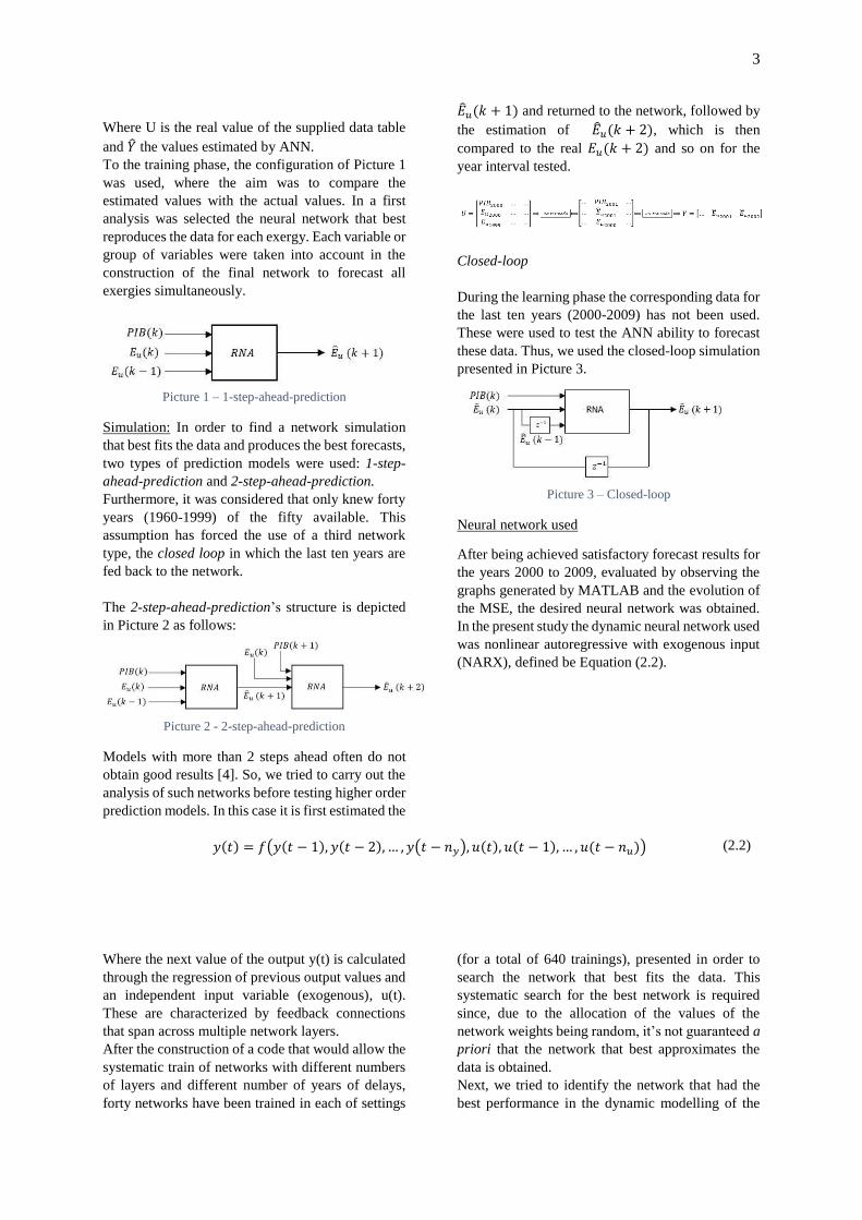
problem. For that, the network with smaller MSE in

bringing data was identified. Nevertheless, the

analysis was accompanied by analysis of a

performance graph showing the MSE value versus

the number of iterations (Picture 4) and performance

of training and testing validation. This analysis is

needed because if the curve increased significantly

before the increase of the validation curve, then it

was possible that some overtraining may had

occurred.

Picture 4 - Performance graph obtained through the

MATLAB

C. Algorithms and Software libraries

This work was performed with the help of MATLAB

which implements various algorithms and methods

commonly used in machine learning. To find the

optimal number of iterations and neurons, an

exhaustive search was performed across the space

containing all possible combinations of iterations

number and nodes number.

III. RESULTS AND DISCUSSION

This chapter presents the main results. Initially, it

will be made an analysis of the data to identify

outliers and thus separate the disparate data from the

remaining data. Afterwards, the data correlation will

be analyzed. After this analysis we will try to

understand the relationship between the variables

and the contribution of each one for the evolution

description of useful exergy per each type of use in

Portugal.

As this analysis is limited to the correlation between

pairs of variables, it is completed with the analysis

of Principal Components in order to find the

variables with major influence in the explanation of

exergies. Based on this conclusions it is then

possible to find a prediction model for 10 years.

A. Data Pre-Processing

Boxplots: In order to work the data with similar

dimensions we first worked in the standardization so

that the data would have null average and unitary

standard deviation.

Without loss of generality, with 𝑥 aleatory variable

with average µ and standard deviation σ, the

standardization is given by the Equation (3.1):

𝑧 =

(𝑥 − µ)

𝜎

(3.1)

As each variable has fairly distinctive dimensions it

is important to make that normalization in order to

minimize subsequent numerical problems.

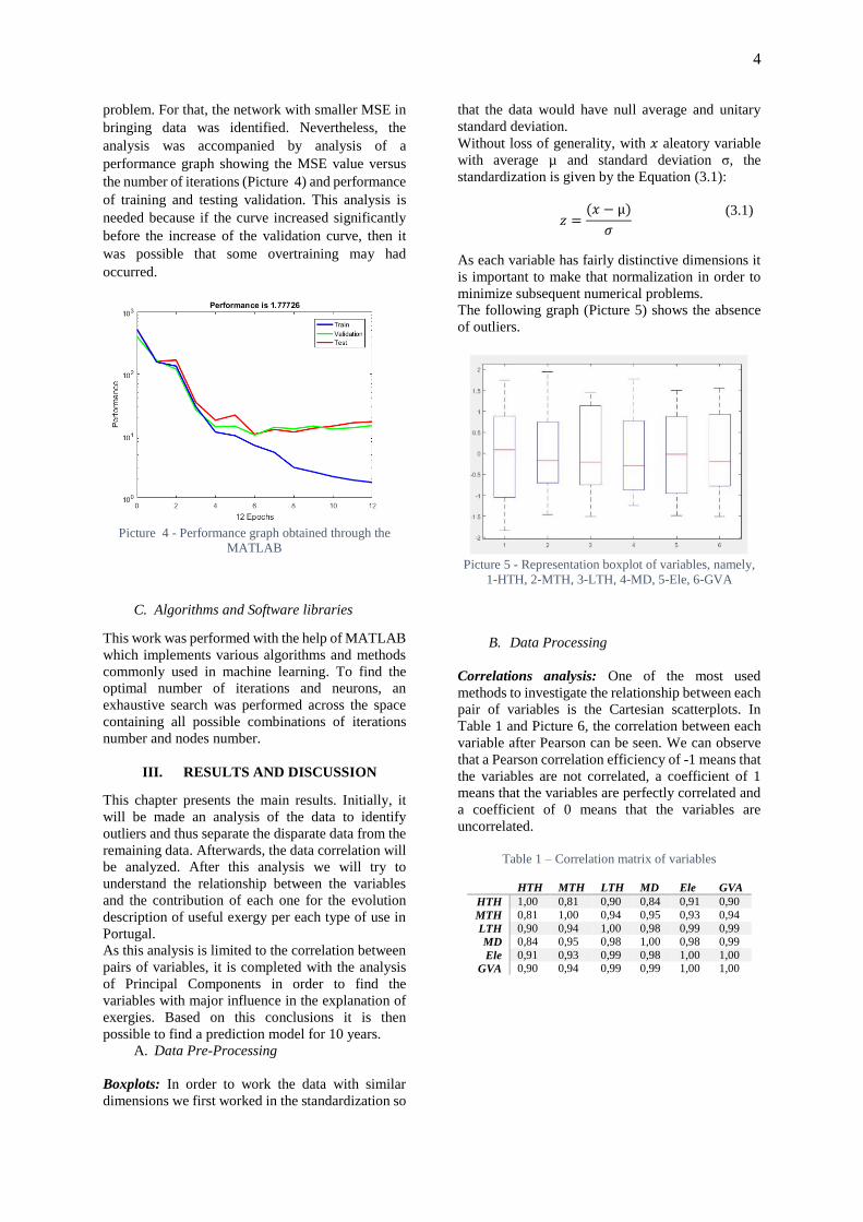
The following graph (Picture 5) shows the absence

of outliers.

Picture 5 - Representation boxplot of variables, namely,

1-HTH, 2-MTH, 3-LTH, 4-MD, 5-Ele, 6-GVA

B. Data Processing

Correlations analysis: One of the most used

methods to investigate the relationship between each

pair of variables is the Cartesian scatterplots. In

Table 1 and Picture 6, the correlation between each

variable after Pearson can be seen. We can observe

that a Pearson correlation efficiency of -1 means that

the variables are not correlated, a coefficient of 1

means that the variables are perfectly correlated and

a coefficient of 0 means that the variables are

uncorrelated.

Table 1 – Correlation matrix of variables

HTH MTH LTH MD Ele GVA

HTH 1,00 0,81 0,90 0,84 0,91 0,90

MTH 0,81 1,00 0,94 0,95 0,93 0,94

LTH 0,90 0,94 1,00 0,98 0,99 0,99

MD 0,84 0,95 0,98 1,00 0,98 0,99

Ele 0,91 0,93 0,99 0,98 1,00 1,00

GVA 0,90 0,94 0,99 0,99 1,00 1,00

5

Picture 6 - Pearson’s correlation

Analyzing the graphic above, the existence of strong

correlations between variables is identified, once the

major part shows correlations values near the unit.

However there are variables such as the HTH and the

MTH that, in spite having the Pearson’s coefficient

relatively lower, have significant dispersions with all

variables when compared to the remaining. This

shows that these variables will be preponderant in

the description of the problem, since they have non-

linear behavior and therefore will add additional

information to the forecast.

PCA analysis: After this, the principal components

were analysed and the significance of each

component variable was observed.

Table 2 demonstrates the covariance matrix which

explains these relationships.

Table 2 – Principal Components of PCA

1ªComp 2ªComp 3ªComp 4ªComp 5ªComp 6ªComp

HTH 0,3840 0,8418 0,2741 -0.0753 -0,2400 -0,0740

MTH 0,3999 -0,4364 0,8023 -0,0386 0,0507 -0,0423

LTH 0,4168 -0,0173 -0,1960 0,8536 0,1683 -0,1747

MD 0,4122 -0,3098 -0,3604 -0,2271 -0,6653 -0.3318

Ele 0,4171 0,0286 -0,2719 -0,4563 0,6844 -0.2730

GVA 0,4183 -0,0614 -0,1971 -0,0658 -0,0228 0,8818

As we can see in the eigenvalues of the shown

covariance matrix in

Table 3, it is verified that the first component has an

eigenvalue of 5.683 and so it describes 94.75% of the

sample. The second component only shows an

eigenvalue of 0.2197, inferior to the unit, the reason

why Elizabeth Reis [2] could not use it in the

analysis.

To select the variables that describe the first

component, the major and/or minor element must be

analysed. In this case, as the column shows very

close values, the major one will be selected better to

represent the corresponding variable GVA.

In the second column three situations are identified:

HTH has a strong positive correlation;

Negative correlations – MTH e MD. The

most negative will be chosen, MTH;

The remaining have a low correlation.

Therefore, for the second component the variables

HTH and MTH will be selected.

In the third component the more negative variable is

selected, i.e., MD. The major element, because it is

related with the variable MTH and since it has

already been selected, will not be taken into account

in this component. Thus, as all the variables have

been around MD, they will be not selected.

In the fourth component, the major variable is again

selected: LTH. Finally, the last choice is Ele with the

most negative value.

In terms of priority in the variables selection for the

description of the problem, we have respectively

GVA, HTH, MTH, MD, LTH and Ele.

Table 3 – Eigenvalues of each principal component

Components Eigenvalues Explation of

variance (%)

Selected

variables

1ª 5,6853 94,7551 GVA

2ª 0,2197 3,6621 HTH e MTH

3ª 0,0758 1,2636 MD

4ª 0,0123 0,2042 LTH e Ele

5ª 0,0049 0,0814 -

6ª 0,0020 0,0336 -

6

Similar to what has been done in the selection

through the correlation matrix, the biplot graphic

was analyzed. It has the components in a system of

axis and the vectors of each of the described

variables in these components are presented. As an

example the first two components in Picture 7 are

presented. Thus, one can visualize the dimension and

the orientation of the variables described in those

principal components, besides reinforcing the

selection of GVA, HTH, MTH and MD.

Picture 7 – Component 1 versus Component 2

C. Development of Prediction Models

ANN: Finally, we identified a model based on

dynamic neural networks. When performing the

training of the network the weight values are

randomly defined. So, the quality of the network for

forecasting also has an inherent randomness. We

proceeded to the training of 640 networks where

various combinations of entry variables were very

often tested with one or two years of delay for the

variables of exergy.

After that analysis the structure (Picture 8) of the

network was identified which gave the best MSE

results and so it was considered to best model and

describe the problem. The entry variables of the

network are: GVA, HTH, MTH, LTH, MD and Ele

and also the latter five delayed one year.

Picture 8 – Network structure removed from MATLAB

In the network structure shown it is observed that the

network receives 6 input variables (x(t)) where 5 of

these variables (y(t)) also come with a year prior to

the prediction:

x(t) = [matrix with variables GVA, HTH, MTH, LTH,

MD and Ele] without delay (represented by 0 of the

“clock” in hidden) and y(t) = [matrix with variables

HTH, MTH, LTH, MD and Ele]. This variable

corresponds to the variables that are one year late, as

these data remains in a cycle (represented by 1 of the

“clock” in hidden) waiting to enter the network.

The network consists of six hidden layers (number 6

in hidden) in which the neurons are modeled by

sigmoid functions and the five required variables are

provided (number 5 in output).

In Picture 9, Picture 10, Picture 11, Picture 12,

Picture 13 the results of the net with 6 hidden layers

and 85 neurons in the hidden layer are presented. In

black we can see the prediction of the first forty years

using the training, validation and testing of the nets

(1-step-ahead-predicition), in green the prediction to

ten years closed loop process and the red points

represent the known data we try to model.

Picture 9 - Second ANN, representation of HTH

Picture 10 - Second ANN, representation of MTH

7

Picture 11 - Second ANN, representation of LTH

Picture 12 - Second ANN, representation of MD

Picture 13 - Second ANN, representation of Ele

On the pictures above we verify that good

approaches were achieved in the data used to train

and validate the network (first 40 years), having a

satisfactory prediction for the next 10 years. It is

observed that the largest absolute prediction errors

do not exceed 5% in some years (e.g. LTH forecast

in 2007), a perfectly acceptable value. Since the first

forty years of training were reached and because the

forty years were used in the network training and

validation it was expected that the model was very

near the mentioned years. However, the last ten years

will hardly reach that approach, since the network

had no information about them during the stage l.

Besides, in these years because each prediction is

found based in years that had already been estimated,

there is an increased number of mistakes every year.

Picture 14 consolidates the previous conclusions.

Another difficulty closely linked to the prevision

years is the abrupt variation of the variables HTH

and MTH which may introduce desirable oscillations

on the remaining variables since they are not

constant.

Picture 14 - Global error of the variables

For the graphic analysis it was concluded that the

error in absolute value displays a random behavior

and the variables that most contribute to the error in

the prediction years are the MTH, MD and Ele.

However, the behavior of Picture 10, Picture 12,

Picture 13 follows the trend of the variables data.

Other models useful in the prediction of the exergy

are the multiple linear regression and the

multivariate linear regression. We observe the

multivariate analysis in order to determine if this

model shows better results. Because it is a

multivariate model it is expected that there is a

coupling between the variables.

D. Comparison between the three prediction

models

From the analysis of the different methods it can be

verified that the neural network was able to reach

values with inferior errors. This fact is essential due

to the nonlinear description given by the sigmoid

function of neurons. Besides, the fact that the net has

an over-definition of the parameters in its structure

provides some flexibility to ANN, being thus

possible to obtain predictions with an order of

magnitude three times inferior in the case of ANN

seen on Table 4.

8

Table 4 – Error comparison of ten years forecast

HTH MTH LTH MD Ele Global Error

Multiple 8,17 × 10−1 2,48 × 10−1 1,99 × 10−1 4,53 × 10−2 1,11 × 10−1 1,57 × 10−1 Multivariate 2,74 × 10−1 3,17 × 10−1 1,58 × 10−1 0,65 × 10−2 0,57 × 10−2 0,40 × 10−1

ANN 4,10 × 10−4 1,46 × 10−4 3,86 × 10−4 5,12 × 10−4 8,25 × 10−4 1,65 × 10−4

No matter what the adopted method is, the training

data is few descriptive of the behavior to predict.

This leads to increased difficulties when

extrapolating. In the case of linear regressions this

made the functions more rigid to present variations

in the last ten years. On the other hand, in case of

ANN this factor caused some overtraining situations,

creating nets which interpolated significantly well

the training years. This led sometimes to

unacceptable responses in years of prediction, or just

the contrary, meaning predictions relatively

acceptable but with the training years having great

alterations and amplitude.

Finally, the graphs (

Picture 15, Picture 16, Picture 17, Picture 18, Picture

19) of the errors of the ten-year forecast for ANN

analysis are shown. It was concluded that in general

terms looking at the sum of the errors, although there

are some years better than others, the graphics

individually approach to the real data. It is noted that

the larger the “web” the greater the error in the

predicted year. If the “web” is small the error is

smaller.

It was concluded, by graphical observation, the

neural network was the forecast model that best

adapted to the data provided, providing very useful

information on the estimates of the variables

individually.

Picture 15 – Error evolution of variables in 2000 and

2001 for the ANN predictive analysis

Picture 16 - Error evolution of variables in 2002 and 2003

for the ANN predictive analysis

Picture 17 - Error evolution of variables in 2004 and 2005

for the ANN predictive analysis

Picture 18 - Error evolution of variables in 2006 and 2007

for the ANN predictive analysis

9

Picture 19 - Error evolution of variables in 2008 and 2009

for the ANN predictive analysis

IV. CONCLUSIONS AND

RECOMMENDATIONS

The aim of this study was to present a new study that

combines the approach of Artificial Neural

Networks (ANN) with the evolution of the useful

exergy in order to forecast energy consumption in

Portugal from 2000 to 2009, providing information

about GVA and of useful exergy such as HTH,

MTH, LTH, MD and Other Electric Uses+Light

(Ele) related to fifty years in Portugal.

In the aid of this data we intent to model and predict

information related to useful exergies per type of

use. However this is a difficult task: neural networks

have demonstrated to be a tool with good capacity

for this process relatively to more conventional

methods such as multiple and multivariate linear

regression, due to its aptitude to distinguish the

relationship existing in a certain amount of data.

Before the construction of the different models, a

pre-treatment of the data and various analysis of

correlations were performed in order to understand

the variables which contribute with more

information for the description of useful exergy and

to reduce the number of variables. We made a

principal components (PCA) analysis to find the

variables with higher influence in the prediction

process, which were defined as net inputs. The

variables that we chose are, by descending order,

GVA, HTH, MTH, MD, LTH and Ele.

In this study the application of dynamic nets with the

Levenberg-Marquardt optimization algorithm was

used. With this methodology it was possible to adjust

the real data for the period between 1960 and 2009.

The best obtained net is composed by 6 hidden

layers, 85 neurons in the hidden layer, the entry

variables GVA, HTH, MTH, LTH, MD and Ele and

the last five delayed one year.

The data concerning the first forty years was used in

the training, testing and validation of the net and the

last ten years were only used for validation. In this

study the net in closed loop was applied. With this

net a value of MSE of 1,65 × 10−4 regarding the

prediction of those ten years was obtained.

In order to verify the quality of the net the results

were compared with models obtained by the multiple

and multivariate linear regression. They have

demonstrated to have an inferior quality when

compared to ANN.

In every case, the difficulty in the extrapolation due

to the behavior discrepancy of the training data (first

forty years) and the prediction of the last ten years

was verified. Those difficulties appear as the lack of

flexibility to the sharp variations in the case of linear

regressions.

As a future study it is important to evaluate the

relationship with other input variables and to test a

new network structure. The neural networks require

a lot of data in order to obtain a model that can well

adjust to each case study, therefore it needs a lot of

inputs to run properly. Hence, a suggestion for future

development is to analyze these variables for a

higher period of time because if the data is larger the

models could have better performances, since the

growth in the data can contribute to obtain better

results in exergy prediction.

This study shows that dynamic neural networks have

good results for exergy prediction and can eventually

be adopted by other countries. Another proposal is to

adapt this dynamic neural network in predicting

other types of consumption, besides energy.

As a final note and based on the article developed for

China [1] it would be interesting to develop a

forecasting study, for e.g. 2030 - 2050, with GVA

scenarios for Portugal and compare it with existing

scenarios.

REFERENCES

[1] Brockway, P. E., Steinberger, J. K., Barrett, J. R.

and Foxon, T. J. (2015). Understanding China´s past

and future energy demand: An exergy efficiency and

decomposition analysis. Applied Energy,

155(2015):892–903.

[2] Elizabeth Reis (2001). Estatística Multivariada

Aplicada. Edições Sílabo.

[3] INE (2015). Anuário Estatístico de Portugal

2012. Relatório Técnico, Instituto Nacional de

Estatística.

[4] Parlos, A.G., Rais, O.T., Atiya, A.F. (2000).

Multi-step-ahead prediction using dynamic recurrent

neural networks. Neural Networks 13 765-786.

[5] Percebois J. (1979). Is the concept of energy

intensity meaningful? Energy Economic.

[6] Pinheiro, M. (ed.) (1997). Séries Longas para a

Economia Portuguesa. Pós II Guerra Mundial, vol. I

- Séries Estatísticas. Lisbon, Banco de Portugal.

[7] Serrenho, A., Sousa, T., Warr, B., Ayres, R.,

Domingos, T. (2014). Decomposition of useful work

intensity: The EU (European Union)-15 countries

from 1960 to 2009. Energy 76 704-715.

[8] Serrenho, A., Warr, B., Sousa, T., Ayres, R.,

Domingos, T. (2015). Structure and dynamics of

useful work along the agriculture-industry-services

10

transition: Portugal from 1856 to 2009. Structural

Change and Economic Dynamics 36 1-21.