neural networks for machine learning lecture 4a learning...

Neural Networks for Machine Learning

Lecture 4a

Learning to predict the next word

Geoffrey Hinton with Nitish Srivastava Kevin Swersky

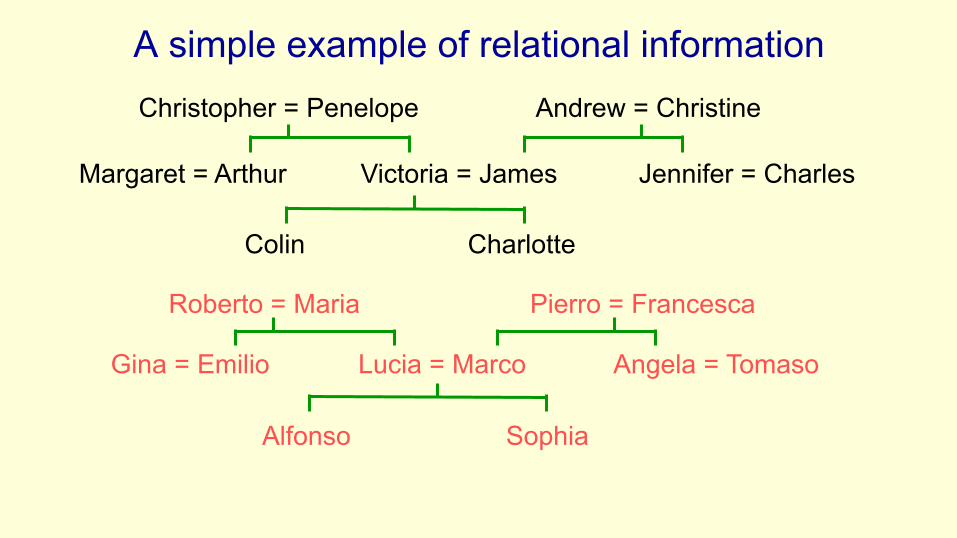
A simple example of relational information Christopher = Penelope Andrew = Christine

Margaret = Arthur Victoria = James Jennifer = Charles

Colin Charlotte

Roberto = Maria Pierro = Francesca

Gina = Emilio Lucia = Marco Angela = Tomaso

Alfonso Sophia

Another way to express the same information •  Make a set of propositions using the 12 relationships:

–  son, daughter, nephew, niece, father, mother, uncle, aunt –  brother, sister, husband, wife

•  (colin has-father james) •  (colin has-mother victoria) •  (james has-wife victoria) this follows from the two above •  (charlotte has-brother colin) •  (victoria has-brother arthur) •  (charlotte has-uncle arthur) this follows from the above

A relational learning task

•  Given a large set of triples that come from some family trees, figure out the regularities. –  The obvious way to express the regularities is as symbolic rules

(x has-mother y) & (y has-husband z) => (x has-father z) •  Finding the symbolic rules involves a difficult search through a very

large discrete space of possibilities. •  Can a neural network capture the same knowledge by searching

through a continuous space of weights?

The structure of the neural net local encoding of person 2

local encoding of person 1 local encoding of relationship

distributed encoding of person 1 distributed encoding of relationship

distributed encoding of person 2

units that learn to predict features of the output from features of the inputs

output

inputs

Christopher = Penelope Andrew = Christine

Margaret = Arthur Victoria = James Jennifer = Charles

Colin Charlotte

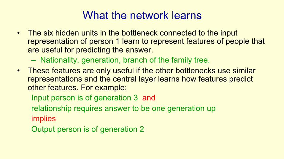
What the network learns •  The six hidden units in the bottleneck connected to the input

representation of person 1 learn to represent features of people that are useful for predicting the answer. –  Nationality, generation, branch of the family tree.

•  These features are only useful if the other bottlenecks use similar representations and the central layer learns how features predict other features. For example: Input person is of generation 3 and relationship requires answer to be one generation up implies Output person is of generation 2

Another way to see that it works

•  Train the network on all but 4 of the triples that can be made using the 12 relationships –  It needs to sweep through the training set many times

adjusting the weights slightly each time. •  Then test it on the 4 held-out cases.

–  It gets about 3/4 correct. –  This is good for a 24-way choice. –  On much bigger datasets we can train on a much smaller

fraction of the data.

A large-scale example •  Suppose we have a database of millions of relational facts of the

form (A R B). –  We could train a net to discover feature vector

representations of the terms that allow the third term to be predicted from the first two.

–  Then we could use the trained net to find very unlikely triples. These are good candidates for errors in the database.

•  Instead of predicting the third term, we could use all three terms as input and predict the probability that the fact is correct. –  To train such a net we need a good source of false facts.


Lecture 4b

A brief diversion into cognitive science


What the family trees example tells us about concepts

•  There has been a long debate in cognitive science between two rival theories of what it means to have a concept:

The feature theory: A concept is a set of semantic features. –  This is good for explaining similarities between concepts. –  Its convenient: a concept is a vector of feature activities.

The structuralist theory: The meaning of a concept lies in its relationships to other concepts. –  So conceptual knowledge is best expressed as a relational graph. –  Minsky used the limitations of perceptrons as evidence against

feature vectors and in favor of relational graph representations.

Both sides are wrong

•  These two theories need not be rivals. A neural net can use vectors of semantic features to implement a relational graph. –  In the neural network that learns family trees, no explicit inference is

required to arrive at the intuitively obvious consequences of the facts that have been explicitly learned.

–  The net can “intuit” the answer in a forward pass.

•  We may use explicit rules for conscious, deliberate reasoning, but we do a lot of commonsense, analogical reasoning by just “seeing” the answer with no conscious intervening steps. –  Even when we are using explicit rules, we need to just see which

rules to apply.

Localist and distributed representations of concepts

•  The obvious way to implement a relational graph in a neural net is to treat a neuron as a node in the graph and a connection as a binary relationship. But this “localist” method will not work: –  We need many different types of relationship and the connections

in a neural net do not have discrete labels. –  We need ternary relationships as well as binary ones.

e.g. A is between B and C. •  The right way to implement relational knowledge in a neural net

is still an open issue. –  But many neurons are probably used for each concept and each

neuron is probably involved in many concepts. This is called a “distributed representation”.


Lecture 4c

Another diversion: The softmax output function


Problems with squared error

•  The squared error measure has some drawbacks: –  If the desired output is 1 and the actual output is 0.00000001

there is almost no gradient for a logistic unit to fix up the error. –  If we are trying to assign probabilities to mutually exclusive class

labels, we know that the outputs should sum to 1, but we are depriving the network of this knowledge.

•  Is there a different cost function that works better? –  Yes: Force the outputs to represent a probability distribution

across discrete alternatives.

Softmax

∂yi∂zi

= yi (1− yi )

The output units in a softmax group use a non-local non-linearity:

softmax group zi

yi

this is called the “logit”

yi =ezi

ezjj∈group∑

Cross-entropy: the right cost function to use with softmax

C = − t j logj∑ yj

•  The right cost function is the negative log probability of the right answer.

•  C has a very big gradient when the target value is 1 and the output is almost zero. –  A value of 0.000001 is much better

than 0.000000001

–  The steepness of dC/dy exactly balances the flatness of dy/dz

target value

∂C∂zi

=∂C∂yj

∂yj∂zij

∑ = yi − ti


Lecture 4d

Neuro-probabilistic language models


A basic problem in speech recognition •  We cannot identify phonemes perfectly in noisy speech

–  The acoustic input is often ambiguous: there are several different words that fit the acoustic signal equally well.

•  People use their understanding of the meaning of the utterance to hear the right words. –  We do this unconsciously when we wreck a nice beach. –  We are very good at it.

•  This means speech recognizers have to know which words are likely to come next and which are not. –  Fortunately, words can be predicted quite well without full

understanding.

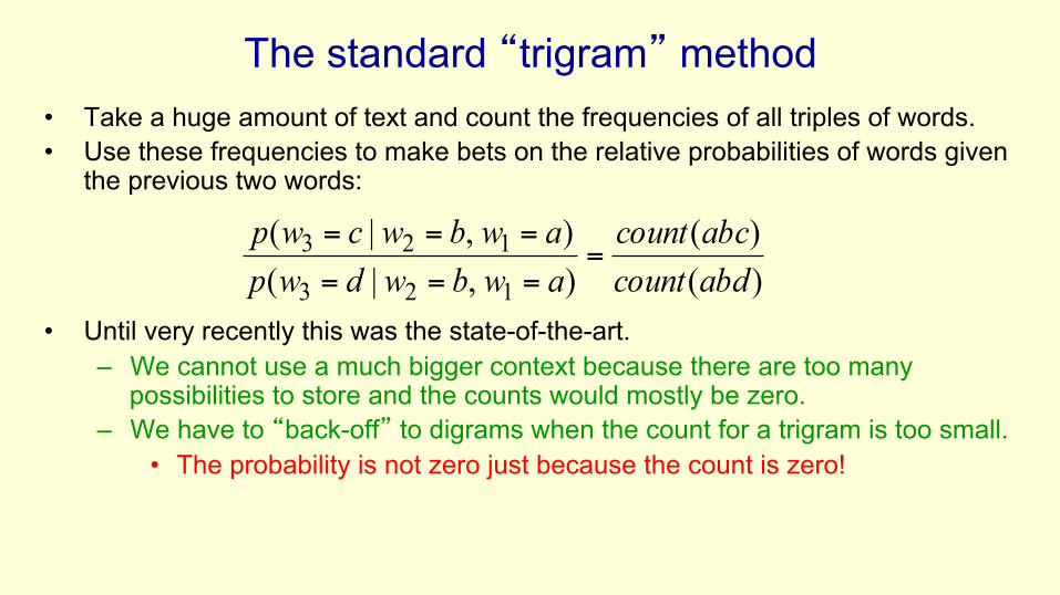
•  Take a huge amount of text and count the frequencies of all triples of words. •  Use these frequencies to make bets on the relative probabilities of words given

the previous two words:

•  Until very recently this was the state-of-the-art. –  We cannot use a much bigger context because there are too many

possibilities to store and the counts would mostly be zero. –  We have to “back-off” to digrams when the count for a trigram is too small.

•  The probability is not zero just because the count is zero!

The standard “trigram” method

)()(

),|(),|(

123

123abdcountabccount

awbwdwpawbwcwp

====

===

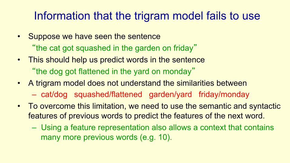
Information that the trigram model fails to use •  Suppose we have seen the sentence “the cat got squashed in the garden on friday”

•  This should help us predict words in the sentence “the dog got flattened in the yard on monday”

•  A trigram model does not understand the similarities between –  cat/dog squashed/flattened garden/yard friday/monday

•  To overcome this limitation, we need to use the semantic and syntactic features of previous words to predict the features of the next word. –  Using a feature representation also allows a context that contains

many more previous words (e.g. 10).

Bengio’s neural net for predicting the next word

“softmax” units (one per possible next word)

index of word at t-2 index of word at t-1

learned distributed encoding of word t-2


units that learn to predict the output word from features of the input words

table look-up table look-up

skip-layer connections

A problem with having 100,000 output words

•  Each unit in the last hidden layer has 100,000 outgoing weights. –  So we cannot afford to have many hidden units.

•  Unless we have a huge number of training cases. –  We could make the last hidden layer small, but then its hard to

get the 100,000 probabilities right. •  The small probabilities are often relevant.

•  Is there a better way to deal with such a large number of outputs?


Lecture 4e

Ways to deal with the large number of possible outputs in neuro-probabilistic language models


A serial architecture



hidden units that discover good or bad combinations of features

learned distributed encoding of candidate

logit score for the candidate word

Try all candidate next words one at a time.

index of word at t-2

table look-up


table look-up

index of candidate

table look-up

This allows the learned feature vector representation to be used for the candidate word.

Learning in the serial architecture

•  After computing the logit score for each candidate word, use all of the logits in a softmax to get word probabilities.

•  The difference between the word probabilities and their target probabilities gives cross-entropy error derivatives. –  The derivatives try to raise the score of the correct candidate

and lower the scores of its high-scoring rivals. •  We can save a lot of time if we only use a small set of candidates

suggested by some other kind of predictor. –  For example, we could use the neural net to revise the

probabilities of the words that the trigram model thinks are likely.

Learning to predict the next word by predicting a path through a tree (Minih and Hinton, 2009)

•  Arrange all the words in a binary tree with words as the leaves.

•  Use the previous context to generate a “prediction vector”, v. –  Compare v with a learned vector,

u, at each node of the tree. –  Apply the logistic function to the

scalar product of u and v to predict the probabilities of taking the two branches of the tree.

ui

uj uk

unumul

1−σ (vTui ) σ (vTui )

σ (vTuj )1−σ (vTuj )

A picture of the learning

ui

uj uk

unumul

1−σ (vTui ) σ (vTui )

σ (vTuj )1−σ (vTuj )learned distributed encoding of word t-2


table look-up



prediction vector, v

w(t)

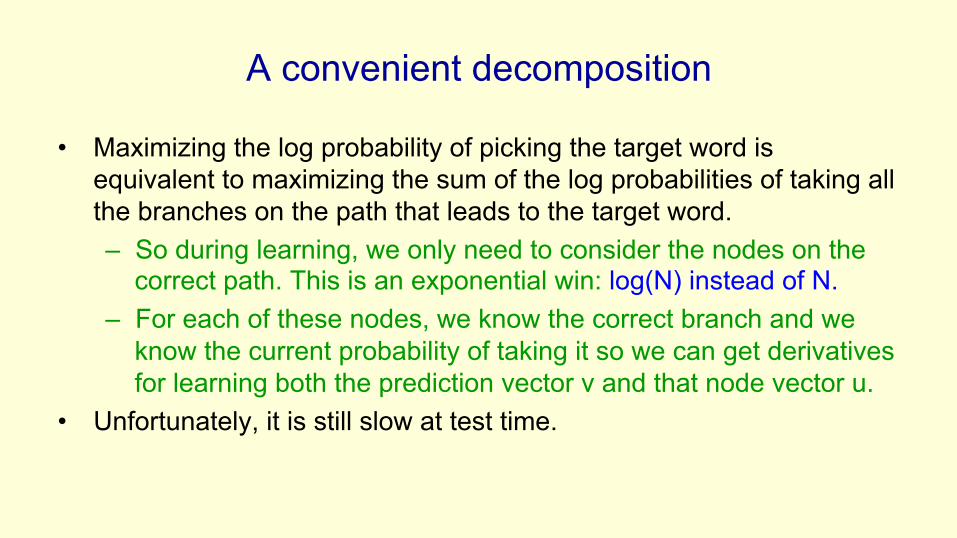
A convenient decomposition

•  Maximizing the log probability of picking the target word is equivalent to maximizing the sum of the log probabilities of taking all the branches on the path that leads to the target word. –  So during learning, we only need to consider the nodes on the

correct path. This is an exponential win: log(N) instead of N. –  For each of these nodes, we know the correct branch and we

know the current probability of taking it so we can get derivatives for learning both the prediction vector v and that node vector u.

•  Unfortunately, it is still slow at test time.

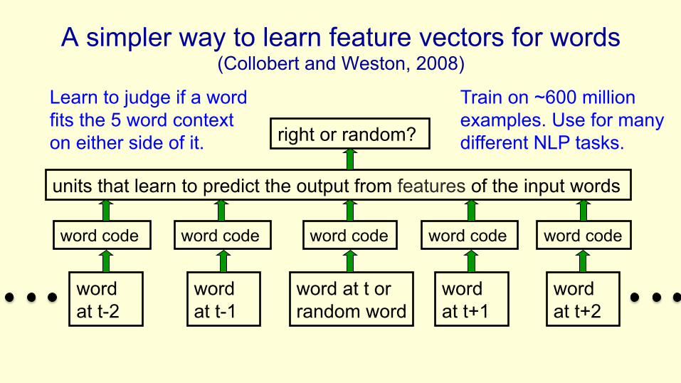
A simpler way to learn feature vectors for words (Collobert and Weston, 2008)

word at t-2

word code

word at t-1

word code

word at t or random word

word code

word at t+1

word code

word at t+2

word code

units that learn to predict the output from features of the input words

right or random?

Train on ~600 million examples. Use for many different NLP tasks.

Learn to judge if a word fits the 5 word context on either side of it.

Displaying the learned feature vectors in a 2-D map

•  We can get an idea of the quality of the learned feature vectors by displaying them in a 2-D map. –  Display very similar vectors very close to each other. –  Use a multi-scale method called “t-sne” that also displays similar

clusters near each other. •  The learned feature vectors capture lots of subtle semantic

distinctions, just by looking at strings of words. –  No extra supervision is required. –  The information is all in the contexts that the word is used in. –  Consider “She scrommed him with the frying pan.”

Part of a 2-D map of the 2500 most common words

neural networks for machine learning lecture 4a learning...

Documents