using gpus for realtime prediction of optical forces on

Proceedings of the ASME 2012 International Design Engineering Technical Conferences &Computers and Information in Engineering Conference

IDETC/CIE 2012August 12-15, 2012, Chicago, IL, United States of America

DETC2012-71236

USING GPUS FOR REALTIME PREDICTION OF OPTICAL FORCES ONMICROSPHERE ENSEMBLES

Sujal BistaGraduate Student

Inst. for Advanced Computer StudiesDepartment of Computer Science

University of MarylandCollege Park, Maryland 20742

Email: [email protected]

Sagar ChowdhuryResearch Assistant

Dept. of Mechanical EngineeringUniversity of Maryland

College Park, Maryland 20742Email: [email protected]

Satyandra K. GuptaProfessor, Fellow of ASMEInst. for Systems Research

Department of Mechanical EngineeringUniversity of Maryland

College Park, Maryland 20742Email: [email protected]

Amitabh VarshneyProfessor

Inst. for Advanced Computer StudiesDepartment of Computer Science

University of MarylandCollege Park, Maryland 20742Email: [email protected]

ABSTRACT

Laser beams can be used to create optical traps that canhold and transport small particles. Optical trapping has beenused in a number of applications ranging from prototyping at themicroscale to biological cell manipulation. Successfully usingoptical tweezers requires predicting optical forces on the parti-cle being trapped and transported. Reasonably accurate theoryand computational models exist for predicting optical forces ona single particle in the close vicinity of a Gaussian laser beam.However, in practice the workspace includes multiple particlesthat are manipulated using individual optical traps. It has beenexperimentally shown that the presence of a particle can cast ashadow on a nearby particle and hence affect the optical forcesacting on it. Computing optical forces in the presence of shadowsin real-time is not feasible on CPUs. In this paper, we introducea ray-tracing-based application optimized for GPUs to calculateforces exerted by the laser beams on microparticle ensembles in

an optical tweezers system. When evaluating the force exertedby a laser beam on 32 interacting particles, our GPU-based ap-plication is able to get a 66-fold speed up compared to a singlecore CPU implementation of traditional Ashkin’s approach anda 10-fold speedup over its single core CPU-based counterpart.

1 IntroductionAn optical tweezers system is a scientific instrument that

uses light to manipulate micron-sized particles. Ashkin first in-troduced the system in 1986 [1]. Since then scientists have beenusing this system to manipulate and study microparticles suchas dielectric spheres, cells, DNA, bacteria, and virus. They areoften used in creating assembly of micro- and nano-scaled com-ponents to make a functional device due to the extensive rangeof positioning and orienting capabilities of the system [2]. Addi-tionally, optical tweezers systems can be used to manipulate cellsin a controlled manner without causing them any damage [3,4,5].

1 Copyright c© 2012 by ASME

FIGURE 1. In an optical tweezer setup, a Gaussian laser beam isconverged by a convex lens (objective lens of a microscope) to a focalpoint which is used for trapping microparticles. To create multiple opti-cal traps, the laser beam is split into multiple-beams using a diffractiongrating. Diagram courtesy of [6].

FIGURE 2. An illustration of the optical tweezers system. A laserbeam with a Gaussian-based intensity distribution is converged into afocal point with the help of a convex lens. The figure shows laser beamtrapping microparticles at the focal point.

The optical tweezers system is composed of a very powerfullaser beam that has a Gaussian-based intensity distribution anda convex lens that focuses the laser beam onto the focal point asshown in Figure 1. This focused laser beam is used to move mi-croparticles that are submerged in the fluid. When the micropar-

ticles are bigger than the wavelength of the light used in the laserbeam, the ray optics model is used to define the behavior of theoptical tweezers system [1]. The laser beam is decomposed intoa bundle of rays, each carrying a photon. When these rays inter-act with the microparticles, they get reflected and refracted. Aseach ray consists of a photon, the change in the momentum givesrise to the optical force that is exerted on the microparticles. Thisforce is used by the optical tweezers system to trap and movethe microparticles. Figure 2 shows an illustration of a micropar-ticle getting trapped. Figure 3 shows a series of images cap-tured through the imaging device in the optical tweezers systemin our lab showing a microparticle (silicon bead) getting trapped.An optical trap is placed close to the microparticle which exertsa strong gradient force that pulls the particle towards the focalpoint.

Simulation plays an important role in understanding opti-cal tweezers system. To manipulate microparticles precisely, theforce exerted by the laser has to be known; this is studied byperforming simulations. The force calculation is a very compu-tationally intensive task due to the Brownian motion of the mi-croparticles suspended in the fluid which requires the time step ofthe simulation to be smaller than 10−6 sec. The popular approachto overcome the timing constraint is to use a pre-computed forcelook-up table to study simulation as done by Banerjee et al. [2].Reasonably accurate theory and computational models exist forpredicting optical forces on a single particle in the close vicinityof the Gaussian laser beam. However, in practice the workspaceincludes multiple particles that are manipulated using individualoptical traps. Experiments have shown that the presence of a par-ticle can cast a shadow on a neighboring particle and hence affectthe optical forces acting on it. When microparticles are closelyplaced under several laser beams, the rays get reflected and re-fracted which introduces secondary forces that affect the trap-ping. This behavior is often referred as shadowing phenomenon.It occasionally causes trapped microparticles to escape or causean unwanted microparticle to jump into the trap. Studying thisphenomenon is vital for scientists who are using optical tweezerssystem for micro assembly or path planning [7, 8, 9].

In this paper, we present an optimized GPU-based ray trac-ing application to calculate the force exerted by the laser beamson the microparticles to study the shadowing phenomenon. Ourprogram is capable of computing the forces exerted by laserbeams on multiple microparticles (up to 32) at more than 100Hzwhich is a higher rate than that of a typical optical device usedfor imaging/monitoring the microparticles. We are able to cal-culate the interaction between the lasers and several microparti-cles and make it possible to study the shadowing phenomenonvital for understanding optical trapping. When evaluating theforce exerted by a laser beam on 32 interacting particles, ourGPU-based application is able to get approximately a 66 timesspeed up compared to a single core CPU implementation of tra-ditional Ashkin’s approach and a 10 times faster than its single


FIGURE 3. When an optical trap is placed close to a microparticle, itpulls the particle towards the focal point. The images above captured us-ing the imaging device in the optical tweezers system show a micropar-ticle moving into a trap.

core CPU-based counterpart. In this paper, we also talk aboutseveral choices we made while developing this application andcompare them in terms of performance and precision. We also

present an alternative way to calculate force exerted by the laserthat exploits coherence of the mapping from incident ray to thex,y,z components of force and the transmitted ray by using non-negative matrix factorization (NMF). This method can be usefulwhen computation of the path a ray travels within the microparti-cle cannot be easily computed by simple sphere-object intersec-tions (possibly caused by uneven density of the microparticle).We also present an instance where the shadowing effect drasti-cally changes the amount of force applied on a microparticle.

2 Related WorkPowerful lasers are used to manipulate microparticles in an

optical tweezers system. This was first introduced by Ashkinet al. [10] where they used a single-beam gradient force to trapmicro- and nano-sized dielectric particles. Ashkin later intro-duced a geometric ray-optic model that is used to compute trap-ping forces created by a laser acting on microparticles muchlarger than the wavelength of light [1]. Though the equationAshkin used is fairly optimized as it computes scattering and gra-dient forces based only on the incident angle and the radial posi-tion of the ray, it only works with rigid spherical objects and can-not be used directly to study interaction between several beamsand microparticles. Our work is focused in calculating forcesusing our GPU-based ray tracing algorithm which provides bothspeed and flexibility needed to study shadowing phenomenon.

One of the biggest challenges in simulating optical tweez-ers system is performing calculation of force exerted by the laserquickly. Since the microparticles are influenced by the Brownianmotion, simulations have to be done at a time scale much smallerthan a microsecond. Banerjee et al. [2] introduced a frameworkwhere offline simulation is used to pre-compute data at discretepoints and is later used to perform fast and accurate calculationof dynamic trapping probability estimates at any arbitrary pointin 3D. This approach cannot accurately compute the effect whenlaser interacts with several nanoparticles. We focus on calculat-ing the force quickly on dynamic microparticles so that the in-teractions of laser with several microparticles can be accuratelysimulated to study the shadowing phenomenon.

Bianchi and Leonardo [11] use GPUs to perform optical ma-nipulation using holograms in real-time. They achieved speedupsof 45X and 350X over CPU on their super position algorithm(SR) and Gerchberg-Saxton weighted algorithm (GSW) respec-tively. The speedup helped them to perform interactive microma-nipulation. Balijepalli et al. [12] and Patro et al. [13] have usedGPUs to compute trapping probabilities and have gotten signif-icant speedups. We also carry out our calculation on the GPU.However our work is focused on computing the force exerted bythe laser beams and we perform ray tracing to compute the forceas the laser interacts with several microparticles.

Sraj et al. [14] used dynamic ray tracing to induce opticalforce on the surface of the deformable cell from which they cal-


culate stress distribution. Rather than using the rigid spheres asan approximated shape of the cell, they perform force calcula-tion on the actual cell. They show that the shape of the cellstrongly influences how the optical force stretches and deformsthem. They also highlight that the applied optical forces changedrastically when the cells are deformed. We focus our study onreducing the amount of time required to compute the exertedforce. We perform our calculation on rigid microparticles andstudy how optical forces change when laser interacts with sev-eral nanoparticles that are closely interacting with each other.

Zhou et al. [15] have introduced a force calculating modelthat uses ray tracing based on spatial analytic geometry. Some ofour ray tracing is based on their work but we perform GPU-basedoptimization and calculate interaction of laser beams with mul-tiple particles quickly which is needed to study the shadowingphenomenon. We also provide an alternative way of computingthe forces using NMF.

Using GPUs to accelerate computationally expensive algo-rithms is gaining a strong interest in the scientific and gamingcommunity. Early work done by Harris et al. [16] used GPUs toperform visual simulation of fluids, clouds, and smoke. Theymapped some basic operators (like heat and Laplace) on theGPU and used these operators to accelerate the simulation. Theyperformed their calculation on the GPU using programmableshaders before general languages for GPU like CUDA, DirectXCompute, and OpenCL became prominent. Considerable ad-vancements in physically-based simulation have been made re-cently due to their application in games and graphics [17]. Inparticular, fluid simulations on GPUs have gained significant mo-mentum [18, 19, 20, 21]. Recently, Phillips et al. [22] used acluster of GPUs to accelerate solver for 2D compressible Eulerequation and MBFLO solvers. Using a cluster of 16 GPUs theyachieve speedups of 496X and 88X on their Euler and MBFLOsolvers. The trend of using GPUs to accelerate existing algo-rithms is growing. In our work, we use GPU-based acclerationof ray tracing to compute the force exerted by the optical tweez-ers on the microparticles.

Carr et al. [23] made a very persuasive case for the use ofGPUs for computing ray-triangle intersections fairly efficientlyby using pixel shaders. Purcell et al. [24] mapped the completeray tracing algorithm to the GPUs, using different pixel shadersfor creating rays, traversing rays, intersecting rays with triangles,and illumination calculations. Another well-known ray tracingengine Optix from NVIDIA uses GPUs for speed. Our ray trac-ing program is similar in nature but rather than calculating colorfor each pixel we compute the force exerted by the laser beam onthe microparticles and perform integration. Also, the density ofrays and the paths taken by the rays used in our calculation aredifferent from the ones used by typical ray tracing program thatuses a pinhole camera model.

FIGURE 4. A diagram showing the simplified ray-optics model forcalculating the force. The incident ray is diverted from its original pathwhen it interacts with the microparticle. This causes the ray to change itsmomentum. When the ray changes momentum due to the microparticle,equal and opposite force is applied to the microparticle.

3 ApproachA simplified ray-optics model for calculating the force is

shown in Figure 4. Due to the change in the index of refrac-tion between the fluid and the microparticle, the incident ray isdiverted from its original path as it goes through the micropar-ticle. This causes the ray to change its momentum. When theray changes momentum, equal and opposite force is applied tothe microparticle. We calculate force contributed by each ray foreach particle. After the contribution of each ray is calculated, in-tegration is done to find the total force. We divide up the entireforce calculation process into several steps described below.

3.1 Ray-Object IntersectionThe first step is to compute fast ray-object intersection. We

compute ray-object intersection on the GPU using a 3D-grid-based data structure. We choose uniform grid-based data struc-ture over BSP, kDTree, and Octree because creating, updating,and ray traversing operation is faster when a uniform 3D gridis used as it allows constant time access to the cells and ray-traversal can be carried out using the efficient 3D-DDA algorithm[25, 24]. In our application, the grid-based data structure is cre-ated on the CPU and sent to the GPU memory every frame. Inthe optical tweezers system, the number of particles monitored inthe experiments is often less than 64, so we create and update thedata structure on the CPU. Once the grid data is transferred to theGPU, we perform ray-object intersection using a GPU Kernel.The ray-object intersection is highly parallelizable and a huge


performance gain is achieved by using many cores of a GPU ascompared to a single core of a CPU. At first we considered us-ing Optix for ray tracing. However we soon realized that weneeded a ray tracer that was more flexible to meet our memorymapping needs, easily integrable with the remaining steps in theforce calculating pipeline, and incurred less overhead. As Optixis a general-purpose ray tracing software made for rendering, wedecided to develop our own dedicated GPU-based program thatis highly specialized for force calculation.

The laser beams are decomposed into RN rays. Each rayis mapped to a thread in the CUDA kernel and all RN threadsare launched at the same time. We save the attributes (such asposition, radius) of the microparticles and the 3D grid data in theglobal GPU memory whereas the properties of the 3D grid andthe laser beam are saved in the constant GPU memory as shownin Figure 5. Every thread traces the path of a ray independently.

3.2 Force CalculationWhen a ray intersects a microparticle, we compute the re-

flected, refracted, and the final transmitted ray by performing ba-sic intersections. Using these rays and the properties of the mi-croparticle, we first compute only the magnitude of the scatteringand the gradient force using the equation described by Ashkin[1].

Fs =n1P

c

{1+Rcos(2θ)− T 2[cos(2θ −2r)+Rcos(2θ)]

1+R2 +2Rcos(2r)

}

Fg =n1P

c

{Rsin(2θ)− T 2[sin(2θ −2r)+Rsin(2θ)]

1+R2 +2Rcos(2r)

}

where n1 is the index of refraction of the incident medium, c isthe speed of light, P is the incident power of the ray, R is theFresnel reflection coefficient, T is the Fresnel transmission coef-ficient, θ is the angle of incidence, and r is the angle of refraction.Then we compute the direction of the scattering and the gradientforces directly from the vectors obtained from ray tracing. Thedirection of the ray is the same as the scattering direction. Forthe gradient direction, we use the scattering direction’s orthogo-nal component that lies on the plane formed by the center of theparticle, the point where the ray intersects the particle, and theintersection of the ray with the horizontal plane as described in[1, 15]. Now using the computed magnitude and the direction,we find the scattering and gradient forces. These forces are com-bined to calculate the total force exerted by the ray. The totalforce is then saved in the GPU memory. The transmitted ray isfurther traced to find the intersection of the ray with other parti-cles and the steps described above are repeated as needed.

FIGURE 5. An overview of the GPU pipeline. The properties ofthe laser and the 3D grid are saved into the constant GPU memorywhereas the properties of the particles and the 3D grid cells are saved inthe global GPU memory. These data are used by the first GPU kernelthat performs ray-object intersection and force per ray calculation. Theoutput is written to a large global memory array. We then perform aparallel-prefix sum at the output. As the parallel-prefix sum adds up allthe components together, Segmentation/Final force calculating kernelfinds the proper segment boundaries for each component and subtractsnecessary amount from the boundaries to compute the final result.


(a) Matrices used in NMF

(b) Non-negative matrix factorization

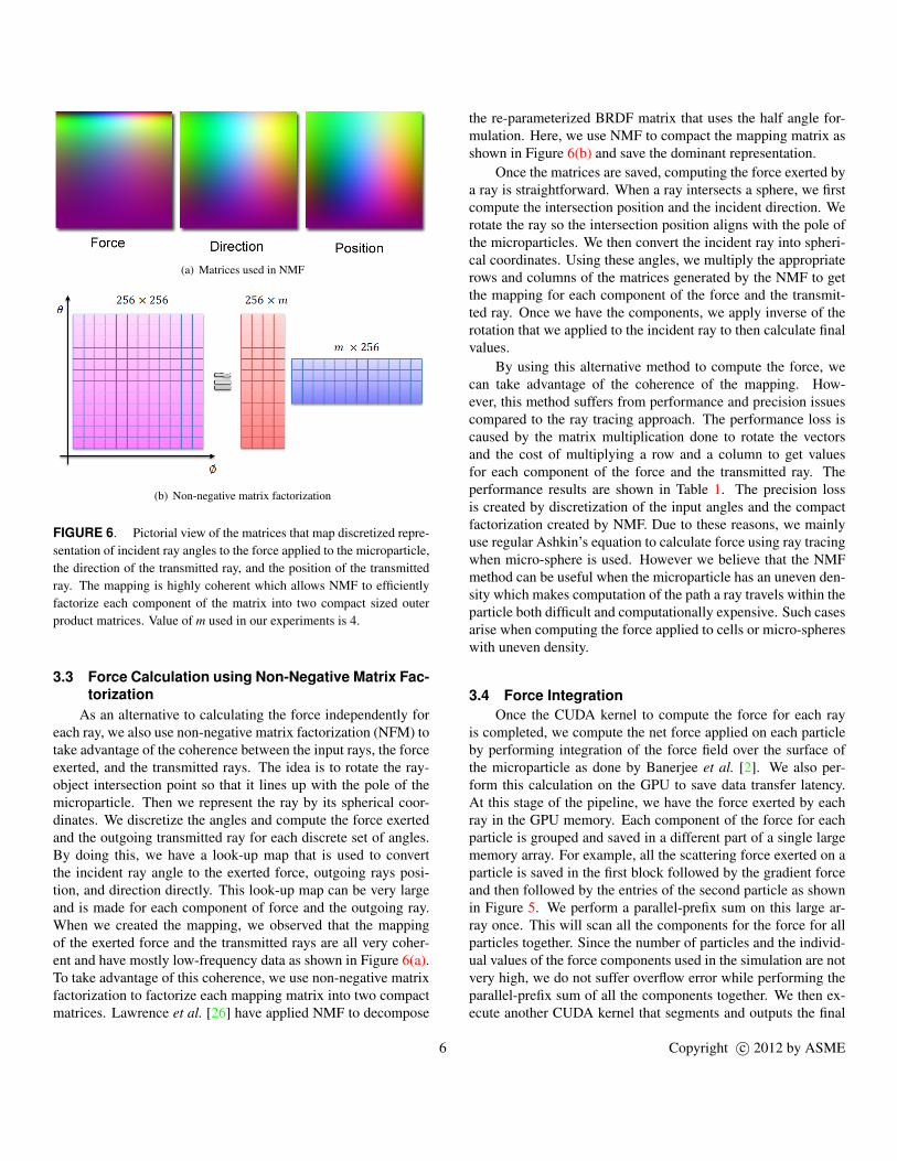
FIGURE 6. Pictorial view of the matrices that map discretized repre-sentation of incident ray angles to the force applied to the microparticle,the direction of the transmitted ray, and the position of the transmittedray. The mapping is highly coherent which allows NMF to efficientlyfactorize each component of the matrix into two compact sized outerproduct matrices. Value of m used in our experiments is 4.

3.3 Force Calculation using Non-Negative Matrix Fac-torization

As an alternative to calculating the force independently foreach ray, we also use non-negative matrix factorization (NFM) totake advantage of the coherence between the input rays, the forceexerted, and the transmitted rays. The idea is to rotate the ray-object intersection point so that it lines up with the pole of themicroparticle. Then we represent the ray by its spherical coor-dinates. We discretize the angles and compute the force exertedand the outgoing transmitted ray for each discrete set of angles.By doing this, we have a look-up map that is used to convertthe incident ray angle to the exerted force, outgoing rays posi-tion, and direction directly. This look-up map can be very largeand is made for each component of force and the outgoing ray.When we created the mapping, we observed that the mappingof the exerted force and the transmitted rays are all very coher-ent and have mostly low-frequency data as shown in Figure 6(a).To take advantage of this coherence, we use non-negative matrixfactorization to factorize each mapping matrix into two compactmatrices. Lawrence et al. [26] have applied NMF to decompose

the re-parameterized BRDF matrix that uses the half angle for-mulation. Here, we use NMF to compact the mapping matrix asshown in Figure 6(b) and save the dominant representation.

Once the matrices are saved, computing the force exerted bya ray is straightforward. When a ray intersects a sphere, we firstcompute the intersection position and the incident direction. Werotate the ray so the intersection position aligns with the pole ofthe microparticles. We then convert the incident ray into spheri-cal coordinates. Using these angles, we multiply the appropriaterows and columns of the matrices generated by the NMF to getthe mapping for each component of the force and the transmit-ted ray. Once we have the components, we apply inverse of therotation that we applied to the incident ray to then calculate finalvalues.

By using this alternative method to compute the force, wecan take advantage of the coherence of the mapping. How-ever, this method suffers from performance and precision issuescompared to the ray tracing approach. The performance loss iscaused by the matrix multiplication done to rotate the vectorsand the cost of multiplying a row and a column to get valuesfor each component of the force and the transmitted ray. Theperformance results are shown in Table 1. The precision lossis created by discretization of the input angles and the compactfactorization created by NMF. Due to these reasons, we mainlyuse regular Ashkin’s equation to calculate force using ray tracingwhen micro-sphere is used. However we believe that the NMFmethod can be useful when the microparticle has an uneven den-sity which makes computation of the path a ray travels within theparticle both difficult and computationally expensive. Such casesarise when computing the force applied to cells or micro-sphereswith uneven density.

3.4 Force IntegrationOnce the CUDA kernel to compute the force for each ray

is completed, we compute the net force applied on each particleby performing integration of the force field over the surface ofthe microparticle as done by Banerjee et al. [2]. We also per-form this calculation on the GPU to save data transfer latency.At this stage of the pipeline, we have the force exerted by eachray in the GPU memory. Each component of the force for eachparticle is grouped and saved in a different part of a single largememory array. For example, all the scattering force exerted on aparticle is saved in the first block followed by the gradient forceand then followed by the entries of the second particle as shownin Figure 5. We perform a parallel-prefix sum on this large ar-ray once. This will scan all the components for the force for allparticles together. Since the number of particles and the individ-ual values of the force components used in the simulation are notvery high, we do not suffer overflow error while performing theparallel-prefix sum of all the components together. We then ex-ecute another CUDA kernel that segments and outputs the final


Number of Rays

Method 82 162 322 642 1282 2562

Ashkin (Float) 0.0759 0.3558 1.2708 5.0548 20.2793 81.7446

Ashkin (Double) 0.0762 0.3705 1.3399 5.3316 21.5276 86.5138

CPU Ray (Float) 0.0807 0.3389 1.4369 5.4946 22.1243 88.9347

CPU Ray (Double) 0.0852 0.3529 1.4268 5.7644 22.8563 92.5199

GPU NMF (Float) 0.9592 0.9589 0.9826 1.1923 2.0615 5.4888

GPU Ray (Float) 0.7132 0.8745 0.8337 0.9007 1.2058 2.3813

TABLE 1. The time in seconds taken by the various methods to compute total force exerted on a single microparticle performed 5000 times atdifferent locations.

force contribution for each particle by subtracting appropriate en-tries from the segment boundaries of each component as shownin Figure 7. This final step performs extremely well on the GPUbecause the output of the previous step is very big so transferringthe data and calculating the final result on the CPU will cause adelay. By calculating the final force contribution on the GPU, weonly need to read back the several components per particle.

FIGURE 7. The final force contribution for each particle is calculatedby subtracting values from the segment boundaries of an array that con-tains the result of the parallel-prefix sum. In this figure, we show howthe final value of the scattering force is computed for a particle.

4 Results and DiscussionWe have implemented our system in C++. We use the

CUDA API for the GPU-based ray tracing. For all of our ex-periments, we use Windows 7 64-bit machine with Intel I5-7502.66 GHz processor, NVIDIA GeForce 470 GTX GPU, and 8GB of RAM.

4.1 Performance ComparisonWe first show the performance gains achieved by using our

GPU-based method. In our first set of experiments, we use rigidmicroparticles and record the amount of time it takes to computethe force. Our performance results are shown in Table 1 and Ta-ble 3. We compare the timings of various methods: Ashkin’straditional, CPU-based ray tracing, GPU-based method that usesNMF, and GPU-based ray tracing methods using single and dou-ble precision floating-point arithmetic. For the first experiment,we perform force calculations on a single microparticle 5000times placed in different locations around the focal point of thelaser beam. We also vary the number of rays that are used todescribe the laser beam. As shown in Table 1, when only onemicroparticle and 2562 rays are used to represent the laser beam,the GPU-based force calculation is about 34 times faster thanAshkin’s method.

Some of the methods we use perform computation on theCPU and some use the GPU. We compare precision betweenvarious methods against CPU-based Ashkin’s method computedusing equal number of rays and double precision floating-pointarithmetic. We perform several comparisons by varying the num-ber of rays to represent the laser beam. The results are shown inTable 2. In general, the relative error decreases as the number ofrays increases. For NMF based computation, the relative errordecreases at first and then fluctuates slightly as we increase thenumber of rays. This is because we discretized input angles whilecreating the mapping table. Due to this, increasing the numberof rays while keeping the size of the mapping table constant, canincrease the amount of error. For regular computations, 322 isan ideal number of rays to use to represent the laser as both therelative error and the computation cost are low.

For the second experiment, we performed force calculationsusing a laser beam and 32 interacting microparticles computed5000 times placed in different locations. The ray tracing methodscan capture the interaction of a laser with multiple particles whileAshkin’s traditional method can only capture interaction of the


laser with a particle at a time ignoring the shadowing effects. Forthe second experiment, we also show the performance differencetriggered by the use of a data structure while doing ray tracing.As shown in Table 3, GPU-based force calculation that uses gridbased data structure is about a 66 times faster than traditionalAshkin’s method and about 10 times faster than its CPU-basedray tracing analog when 2562 rays are used to represent the laserbeam.

When inspected carefully, using a 3D grid causes a slightdelay when the numbers of rays or particles are low. As shownin Figure 8, when the numbers of rays or particles increases, the3D grid performs better than the brute-force ray tracing method.This is generally because of the overhead of creating, updating,and transferring the grid to the GPU. As the performance de-pends on the number of particles, we allow the user to select anydesired method.

4.2 Shadowing PhenomenonWe perform simple experiments to show the shadowing phe-

nomenon. In the traditional ray-tracing community, the phe-nomenon we are simulating would be called as the second andhigher-order refractions. However, since this is referred to as theshadowing phenomenon by the optical tweezers community, thisis the term we shall use here.

We use two microparticles for these experiments. The firstmicroparticle is moving in a path. The second microparticle isstationary and is being gripped by two laser beams with one focalpoint exactly above and the other below the microparticle. Therays that are incident on the second microparticle get refractedwhich can influence the number of rays that interact with thefirst microparticle. Thus the presence of the second microparticlecauses a change in the amount of force being applied to the firstmicroparticle. We show this change by performing simulations.

In the first experiment, we first perform the simulation usinga single silicon bead of size 5 microns. Three Gaussian laser

Number of Rays

Method 82 162 322 642 1282 2562 5122

GPU NMF (Float) 0.0068 0.0047 0.0034 0.0028 0.0035 0.0025 0.0032

CPU Ray (Double) 0.0001 0.0001 0.0001 0.0001 0.0001 0.0001 0.0001

CPU Ray (Float) 0.0005 0.0001 0.0001 0.0001 0.0002 0.0001 0.0001

GPU Ray (Float) 0.0005 0.0006 0.0005 0.0005 0.0005 0.0005 0.0005

TABLE 2. Here we show the comparison of precision between various methods rounded up to the nearest 4 digits. We take Ashkin’s method as thereference and compute the relative error to compare other methods with an equal number of rays. As the number of rays increase, the relative errordecreases in general but the computational cost increases.

Number of Rays

Method 82 162 322 642 1282 2562

Ashkin (Float) 1.8877 7.7762 31.5119 128.1370 515.1390 2081.6000

Ashkin (Double) 1.7971 7.7572 32.0977 129.2160 519.8880 2101.7000

CPU Ray (Float) 0.2951 1.2400 5.1456 21.4900 86.4165 346.2620

CPU Ray (Double) 0.3103 1.3025 5.9534 23.8178 95.1179 379.2980

CPU Ray with 3D Grid (Double) 0.3831 1.3404 5.7862 22.8523 90.7224 360.8080

GPU NMF (Float) 1.3050 2.0442 3.5816 9.1022 30.7739 116.5450

GPU Ray (Float) 1.2649 1.6148 1.9824 3.7576 9.9187 33.3911

GPU Ray with 3D Grid (Float) 1.8859 1.8621 2.2662 3.6953 9.4589 31.5070

TABLE 3. The time taken (in seconds) by the various methods to compute total force exerted by a laser beam on 32 interacting microparticlescomputed 5000 times at different locations. It is interesting to note that when the number of rays is low, brute-force ray tracing is faster than the raytracing method that uses a 3D grid data structure. This is due to the cost of creating and maintaining the data structure.


FIGURE 8. Here we show the time taken to compute the force ex-erted by a laser beam containing 32 rays 5000 times on a varying numberof particles. We compare brute-force GPU ray tracing against GPU raytracing with a 3D grid. As the number of particles increases, the use ofa 3D grid data structure shows a clear advantage.

beams each focused at locations (0.0,0.0,0.0), (−1.0,7.5,0.0),and (−1.0,2.5,0.0) are used. A bead is placed at (0.0,−4.0,0.0)and it slowly moves to (0.0,0.0,0.0). In Figure 9, we show theforce experienced by the bead as it goes from (0.0,−4.0,0.0) to(0.0,0.0,0.0).

Now to show the shadowing phenomenon, we add an ex-tra bead at location (−1.0,5.5,0.0) in the same setup describedabove. This bead acts like a lens and changes the direction ofthe rays from the lasers. This causes the first bead to experienceforce from secondary rays. We compute the force experienced bythe bead as it goes from (0.0,−4.0,0.0) to (0.0,0.0,0.0) whenthe shadowing phenomenon is occurring. In Figure 9, we showthe difference in the amount of force experienced by the first mi-croparticle. This change adds instability and weakens the traps.Now again, we do the similar experiment but this time movethe bead from (−4.0,0.0,0.0) to (0.0,0.0,0.0). Figure 10 showsthe result of force calculation with and without the shadow phe-nomenon.

In both experiments, shadowing effects changes force ap-plied significantly. This can change the behavior of the opti-cal traps. Experimentally validating the results of simulationsis challenging. There is no direct way to measure force. Theforce needs to be inferred from the observed motion. This re-quires a high speed image capture, accounting for the Brownianmotion, and accounting for image blurring due to motion in thez-direction. We are currently in the process of designing experi-ments to record particle trajectories in the presence and absence

(a) Focal point of three laser beams

(b) Single microparticle moving in Y axis

(c) Multiple microparticle with one bead mov-ing in Y axis

(d) Force comparision

FIGURE 9. An illustration of the shadowing phenomenon. Figure (a)shows the focal point of three laser beams at location (0.0,0.0,0.0),(−1.0,7.5,0.0), and (−1.0,2.5,0.0). Figure (b) shows the movementof a single particle from (0.0,−4.0,0.0) to (0.0,0.0,0.0). The Fig-ure (c) shows the movement of same particle when second particle ispresent at location (−1.0,5.5,0.0). Finally, Figure (d) shows the dif-ference in force experienced by the first bead caused by the shadowingphenomenon.


of shadowing phenomena.

(a) Single microparticle moving in X axis

(b) Multiple microparticle with one bead moving in X axis

(c) Force comparision

FIGURE 10. An illustration of the shadowing phenomenon similarto the previous figure. Figure (a) shows the movement of a single par-ticle from (−4.0,0.0,0.0) to (0.0,0.0,0.0). The Figure (b) shows themovement of same particle when second particle is present at location(−1.0,5.5,0.0). Finally, Figure (c) shows the difference in force expe-rienced by the first bead caused by the shadowing phenomenon.

5 Conclusion and Future WorkThe GPU-based application we presented in this paper com-

putes the forces when laser beams interact with multiple mi-croparticles and allow a scientist to study the shadowing phe-nomenon. Studying these phenomenon in real-time is vital asit allows efficient planning required for trapping and manipulat-ing microparticles. When evaluating the force exerted by a laserbeam on 32 interacting particles, our GPU-based application isable to get approximately a 66-fold speed up compared to the sin-gle core CPU implementation of traditional Ashkin’s approachand 10-fold speedup over its single core CPU-based counterpart.We also present an alternative way to calculate the force exertedby the laser that exploits coherence of the mapping from incidentray to the components of force and the transmitted ray by usingNMF.

In future we plan to perform experimental investigation tovalidate our computational model by performing tests on scenar-ios that can be validated experimentally. Currently every timestep is computed independently. Computing the force over a fewtime steps by taking account of changes might provide furtherspeedup.

6 AcknowledgmentThis work has been supported in part by the NSF grants:

CCF 04-29753, CNS 04-03313, CCF 05-41120 and CMMI 08-35572. We also gratefully acknowledge the support provided bythe NVIDIA CUDA Center of Excellence award to the Univer-sity of Maryland. Any opinions, findings, conclusions, or recom-mendations expressed in this article are those of the authors anddo not necessarily reflect the views of the research sponsors.

REFERENCES[1] Ashkin, A., 1992. “Forces of a single-beam gradient laser

trap on a dielectric sphere in the ray optics regime”. Bio-physical Journal, 61, Feb., pp. 569–582.

[2] Banerjee, A. G., Balijepalli, A., Gupta, S. K., and LeBrun,T. W., 2009. “Generating Simplified Trapping Probabil-ity Models From Simulation of Optical Tweezers System”.Journal of Computing and Information Science in Engi-neering, 9, p. 021003.

[3] Koss, B., Chowdhury, S., Aabo, T., Losert, W., and Gupta,S. K., 2011. “Indirect optical gripping with triplet traps”. J.Opt. Soc. America B, 28(5), Apr., pp. 982–985.

[4] Banerjee, A. G., Chowdhury, S., Losert, W., and Gupta,S. K., 2011. “Survey on indirect optical manipulation ofcells, nucleic acids, and motor proteins”. J. Biomed. Opt.,16(5), May.

[5] Chowdhury, S., Svec, P., Wang, C., Losert, W., and Gupta,S. K., 2012. “Robust gripper synthesis for indirect manipu-


lation of cells using holographic optical tweezers”. In IEEEInt. Conf. Intell. Robot. Autom.

[6] Grier, D. G., 2003. “A revolution in optical manipulation”.Nature, 424, Aug., pp. 810–816.

[7] Banerjee, A. G., Pomerance, A., Losert, W., and Gupta,S. K., 2010. “Developing a Stochastic Dynamic Program-ming Framework for Optical Tweezer-Based AutomatedParticle Transport Operations”. IEEE Trans. Autom. Sci.Eng. , 7(2), Apr., pp. 218–227.

[8] Banerjee, A. G., Chowdhury, S., Losert, W., and Gupta,S. K., 2011. “Real-time path planning for coordinatedtransport of multiple particles using optical tweezers”.IEEE Trans. Autom. Sci. Eng. Accepted for publication.

[9] Chowdhury, S., Svec, P., Wang, C., Seale, K., Wikswo,J. P., Losert, W., and Gupta, S. K., 2011. “Investigationof automated cell manipulation in optical tweezers-assistedmicrofluidic chamber using simulations”. In Proc. ASMEInt. Des. Eng. Tech. Conf. & Comp. Inf. Eng. Conf.

[10] Ashkin, A., Dziedzic, J. M., Bjorkholm, J. E., and Chu, S.,1986. “Observation of a single-beam gradient force opticaltrap for dielectric particles”. Optics Letters, 11(5), May,pp. 288–290.

[11] Bianchi, S., and Leonardo, R. D., 2010. “Real-time opticalmicro-manipulation using optimized holograms generatedon the GPU”. Computer Physics Communications, 181(8),pp. 1444–1448.

[12] Balijepalli, A., LeBrun, T., and Gupta, S. K., 2010.“Stochastic Simulations With Graphics Hardware: Char-acterization of Accuracy and Performance”. Journal ofComputing and Information Science in Engineering, 10,p. 011010.

[13] Patro, R., Dickerson, J. P., Bista, S., Gupta, S. K., andVarshney, A., 2012. “Speeding Up Particle Trajectory Sim-ulations under Moving Force Fields using GPUs”. ASMEJournal of Computing and Information Science in Engi-neering. Accepted for publication.

[14] Sraj, I., Szatmary, A. C., Marr, D. W. M., and Eggleton,C. D., 2010. “Dynamic ray tracing for modeling opticalcell manipulation”. Opt. Express, 18(16), Aug, pp. 16702–16714.

[15] Zhou, J.-H., Ren, H.-L., Cai, J., and Li, Y.-M., 2008. “Ray-tracing methodology: application of spatial analytic geom-etry in the ray-optic model of optical tweezers”. AppliedOptics, 47.

[16] Harris, M. J., Coombe, G., Scheuermann, T., and Las-tra, A., 2002. “Physically-based visual simulation ongraphics hardware”. In Proceedings of the ACM SIG-GRAPH/EUROGRAPHICS conference on Graphics hard-ware, HWWS ’02, Eurographics Association, pp. 109–118.

[17] Owens, J. D., Luebke, D., Govindaraju, N., Harris, M.,Kruger, J., Lefohn, A. E., and Purcell, T., 2007. “Asurvey of general-purpose computation on graphics hard-

ware”. Computer Graphics Forum, 26(1), pp. 80–113.[18] Harris, M., 2005. “Fast fluid dynamics simulation on

the GPU”. In SIGGRAPH ’05: ACM SIGGRAPH 2005Courses, ACM, p. 220.

[19] Li, W., Wei, X., and Kaufman, A. E., 2003. “Implementinglattice boltzmann computation on graphics hardware”. TheVisual Computer, 19(7-8), pp. 444–456.

[20] Liu, Y., Liu, X., and Wu, E., 2004. “Real-time 3D fluidsimulation on GPU with complex obstacles”. In PacificConference on Computer Graphics and Applications, IEEEComputer Society, pp. 247–256.

[21] Wei, X., Zhao, Y., Fan, Z., Li, W., Qiu, F., Yoakum-Stover,S., and Kaufman, A. E., 2004. “Lattice-based flow fieldmodeling”. IEEE Transactions on Visualization and Com-puter Graphics, 10(6), pp. 719–729.

[22] Phillips, E. H., Zhang, Y., Davis, R. L., and Owens, J. D.,2009. “Rapid aerodynamic performance prediction on acluster of graphics processing units”. In AIAA AerospaceSciences Meeting, no. AIAA 2009-565.

[23] Carr, N. A., Hoberock, J., Crane, K., and Hart, J. C., 2006.“Fast GPU ray tracing of dynamic meshes using geom-etry images”. In Graphics Interface, Canadian Human-Computer Communications Society, pp. 203–209.

[24] Purcell, T. J., Buck, I., Mark, W. R., and Hanrahan, P.,2002. “Ray tracing on programmable graphics hardware”.ACM Transactions on Graphics, 21(3), July, pp. 703–712.

[25] Fujimoto, A., Tanaka, T., and Iwata, K., 1986. “Arts: Ac-celerated ray-tracing system”. IEEE Computer Graphicsand Applications, 6, pp. 16–26.

[26] Lawrence, J., Rusinkiewicz, S., and Ramamoorthi, R.,2004. “Efficient BRDF importance sampling using a fac-tored representation”. ACM Transactions on Graphics, 23,pp. 496–505.

[27] James, G., 2001. Operations for hardware-accelerated pro-cedural texture animation. Charles River Media, pp. 497–509.

[28] Hagen, T. R., Lie, K.-A., and Natvig, J. R., 2006. “Solv-ing the Euler equations on graphics processing units.”. InInternational Conference on Computational Science (4),pp. 220–227.

[29] Juba, D., and Varshney, A., 2008. “Parallel stochastic mea-surement of molecular surface area”. Journal of MolecularGraphics and Modelling, 27 No. 1, August, pp. 82 – 87.

[30] Heidrich, W., Westermann, R., Seidel, H.-P., and Ertl, T.,1999. “Applications of pixel textures in visualization andrealistic image synthesis”. In Symposium on Interactive3D graphics, ACM, pp. 127–134.


using gpus for realtime prediction of optical forces on

Documents