Using Customers’ Reported Forecasts to Predict

Future Sales

Nihat Altintas †, Alan Montgomery ‡, Michael Trick ‡

Tepper School of Business,

Carnegie Mellon University, Pittsburgh, PA 15213.

†nihat@andrew.cmu.edu

‡alan.montgomery,trick@cmu.edu

May 12, 2006

Abstract

We consider a supplier who must predict future orders using forecasts provided by

their customers. Our goal is to improve the supplier’s operations through a better un-

derstanding of the customers’s forecast behavior. Unfortunately, customer forecasts

cannot be used directly. They may be biased since the customer may want to mislead

the supplier into believing that orders may be larger than expected to secure favorable

terms or simply because the customer is a poor forecaster. There are several unusual

elements in our problem. Analysts typically observe the actual process which may be

biased due to asymmetric loss function. Also units are discrete not continuous. We

believe the forecasting process can be modeled in a multi stage process. The customer

first computes the distribution of demand at a future date which we assume to follow

an ARMA(1,1) model. The customer then submits an integral forecast(multiples of

lot sizes), which minimizes his expected loss due to forecast errors. We show that

the customer may bias his forecasts under an asymmetric loss functions. We provide

an estimator which can be used by the supplier to estimate the forecast generation

model of the customer by looking at his forecasts.

1

1 Introduction

In the last two decades, business environments are undergoing rapid changes due to expan-

sion of computer resources. Companies can now share huge amount of information across

their supply chains. Empowered with the information, companies have a large spectrum

of choices to create complex products and processes. Due to increasing complexity, we ob-

serve more collaborative effort between the different parties in the supply chain. To achieve

higher returns, suppliers and customers invest in technologies that provide real-time access

to demand, inventory, price, sourcing, and production data. Sharing information is key to

increase the profits under demand uncertainty. A critical factor that determines the qual-

ity of information transmission is its reliability. Inaccurate information can lead to severe

costs for the parties in the supply chain. Most of the existing methods are not appropriate

because of the potential bias in the forecasts. However, the suppliers still collect forecasts

from the customers and do not only use their own forecasts. The biased forecasts still

contain information which might be useful for the supplier. It is critical for the supplier to

detect the bias and predict the future order of a customer.

We provide an empirical study about forecast sharing in the supply chains. We analyze the

forecasts of final orders that are received by an automotive supplier who produces multiple

parts for auto manufacturers. Forecast information helps the supplier to predict the final

orders to do production planning in advance. As part of the collaborative effort, customers

provide forecast updates to the supplier at different order dates.

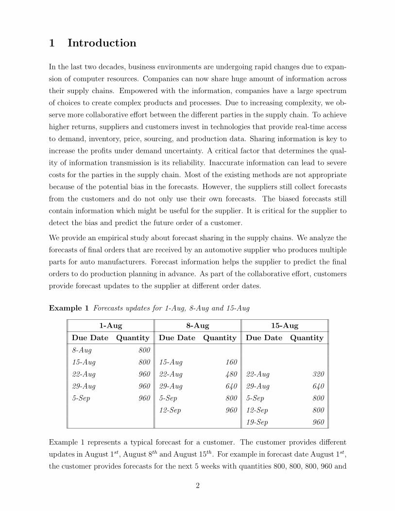
Example 1 Forecasts updates for 1-Aug, 8-Aug and 15-Aug

1-Aug 8-Aug 15-Aug

Due Date Quantity Due Date Quantity Due Date Quantity

8-Aug 800

15-Aug 800 15-Aug 160

22-Aug 960 22-Aug 480 22-Aug 320

29-Aug 960 29-Aug 640 29-Aug 640

5-Sep 960 5-Sep 800 5-Sep 800

12-Sep 960 12-Sep 800

19-Sep 960

Example 1 represents a typical forecast for a customer. The customer provides different

updates in August 1st, August 8th and August 15th. For example in forecast date August 1st,

the customer provides forecasts for the next 5 weeks with quantities 800, 800, 800, 960 and

2

960. In each forecast date, the customer updates the forecasts from the previous forecast

date and can place new orders. Therefore, the forecasts can be considered as a flow of orders

which evolve over time. As can be noticed from the forecast values, due to production and

transportation constraints the customer provides forecasts which are multiples of some lot

sizes. Therefore, we can divide all the forecast by a common divisor (160) to obtain the

number of batches in each order. In this analysis, we propose a framework for modeling

the forecast generation process at the customer.

Forecasts provide information about the future orders of the customer. However, the fore-

cast information can be quite noisy and can be misleading for the supplier. It is critical for

the supplier to process the forecasts to estimate future orders. Altintas and Trick (2004)

study a similar data set in a non-parametric framework and provide empirical support for

downstream players consistently over- or under-estimating their forecasts through time. It

is important for a supplier to recognize a significant pattern in the forecasts by looking

at order history of a customer. Our objective here is to provide a framework to extract

information from the forecast data and adjust the forecasts to provide a better estimate

of future orders. For example, if a customer constantly overestimates his orders, then the

supplier can detect this behavior and can remove the bias from the forecast.

Why do customers provide poor forecast performance?

There are a couple factors that can lead to forecast errors.

1. Uncertainty in the usage: There is always uncertainty in the customer’s system

due to demand variance, lead times, machine failures and etc. Therefore, the error

in the forecast can be a result of these factors. As the due date approaches, the

customer has more information about the demand and uncertainty decreases.

2. Bias in the forecast: The customer can have different costs for overestimation

and underestimation. When the customer overestimates, the supplier can penalize

the customer or the customer can lose the goodwill of the supplier. In the case of

underestimation, the customer cannot satisfy the demand which can lead to delays

in production and potentially lost sales. The customer must consider the trade off

between overestimation and underestimation and submit a forecast which minimizes

the expected cost. The unit overestimation cost is not necessarily equal to underes-

timation cost, therefore the customer may add a bias to his forecast to minimize his

cost.

Therefore a realistic model should consider the uncertainty in production and bias in the

forecast.

3

1.1 Literature Review

Forecasting has been addressed in many different problem settings. There is huge body

of literature in forecasting new observations. In our analysis, the suppliers collect self-

reported forecasts which might be biased from the customers. We use a bayesian approach

to estimate the model parameters in our analysis. Geweke and Whiteman (2006) provide an

extensive review of literature in bayesian forecasting models. Another stream of research

which deals with self-reported forecasts is consensus forecasting models. Batchelor and

Dua (1995) ) show that combinations of different forecasts even from a small number of

sources is helpful in predicting future values. In our case, we have regular updates from

the customers which are combined to predict the customer demand. Therefore, the final

prediction incorporates different updates of the customer.

In our analysis, we model the demand function as a time-series process. The customer

submits his final forecast after considering the cost of overestimation and underestimation.

Time-series assumption has been also used by some other researchers to provide theoretical

results about forecasting. Graves (1999) assumes a non-stationary demand with ARIMA

process and shows that inventory decisions behaves much differently compared to a sta-

tionary process. Aviv (2003) proposes a unified time-series framework for forecasting and

inventory control. He assumes that different parties observe different subsets of informa-

tion, and adopt their forecasting and demand process accordingly. Aviv (2001, 2002) also

study models with time-series demand. Our results provide an empirical support for fore-

casting models which assume strategic behavior of parties with private information in a

time-series framework. Chen et al. (2000a, 2000b) assumes that downstream player uses

moving average forecasts to place orders to a supplier. They measure the amplification in

the variance of the orders which is known as bullwhip effect.

There are other mathematical models in literature for the evolution of demand. Graves et

al. (1986a, 1986b, 1998) and Heath and Jackson (1994) develop the Martingale Model of

Forecast Evolution (MMFE) to model the evolution of forecasts. In MMFE, a forecaster

creates forecasts for the planning horizon and update them in regular intervals. The error

of the forecast updates are assumed to follow the Martingale Property: independent, iden-

tically distributed, multivariate normal random variables with mean 0. MMFE approach

has been studied by a number of researchers under different problem settings. (see, e.g.,

Gullu (1996) , Graves et al. (1998), and Toktay and Wein (2001) ). Another approach

is considering that some demand parameters are unknown in advance and using Bayesian

updates to incorporate new information as it becomes available (Scarf (1959) , Azoury

(1985) and Lariviere and Porteus (1999) )

4

Our analysis has several aspects that have not been addressed in the literature using self-

reported forecasts. First, we assume a loss function for the forecast errors and explain

the dynamics behind the loss function by using a time-series demand. Our analysis is the

first to put the ARIMA form into a newsvendor framework with a cost of overestimation

and underestimation. Second, we assume forecast values which are discrete values since

they are multiples of lot sizes. Third, we provide a statistical procedure to estimate the

model parameters for this complicated problem. A limitation is that we will not get into a

symmetric game, where customer adjusts to the suppliers and vice versa.

The empirical research about forecasting is very limited in the supply chain literature.

Terwiesch et al. (2003) considers the problem from a buyer’s perspective. They demonstrate

that poor forecast performance, in terms of forecast inflation and volatility, damages the

buyer’s reputation and leads to a lower service. In our analysis, we looked at the problem

from the supplier’s perspective and provide analysis to understand the forecast behavior of

the customers.

2 Problem Environment

In our analysis, we model the orders that are placed to an automotive parts supplier by

auto customers. Customers place some preliminary orders (forecasts) starting from six

month before the order date and adjust the forecasts before the due date. The parts are

engine systems and generate multi-billion dollar revenue for the supplier. The customer

has a better ability to predict the demand due to its proximity to the final demand. The

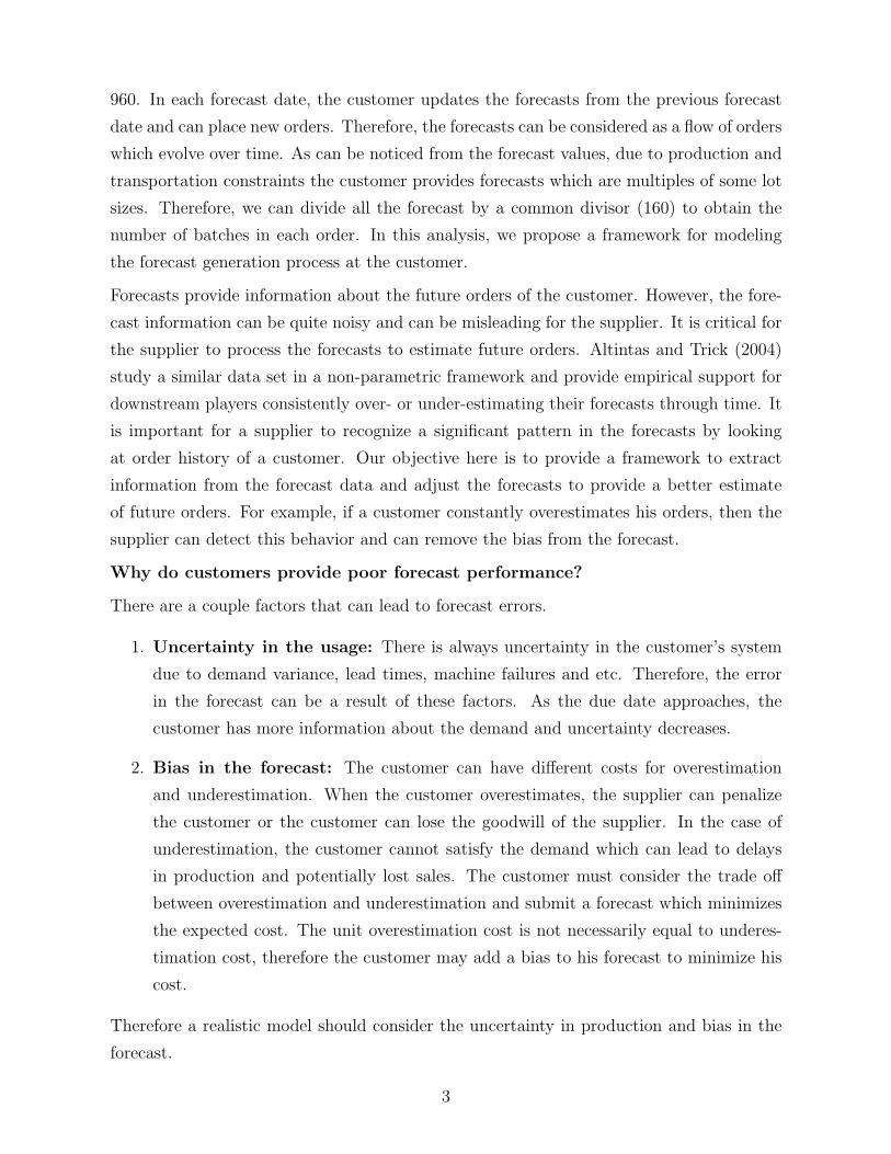
supplier can only observe the forecasts submitted by the customer. In Figure 1, we can see

that the manufacturers provide different updates at 1-Aug, 8-Aug and 15-Aug for the next

5 weeks.

2.1 Demand Model

In our analysis, we observe that the forecasts and forecast errors are autocorrelated through

time. between the periods. A forecast error leads to excess inventory or backordering and

carried to the next period. Another important factor is the autocorrelation between the

demand values of consecutive periods. For example, high demand periods can be followed

with low demand. Therefore, the demand model should be fairly adaptive in order to

incorporate the available information in each period. ARMA model provide a flexible model

to describe different demand processes. (Box and Jenkins 1970) Let Xt as the demand of

5

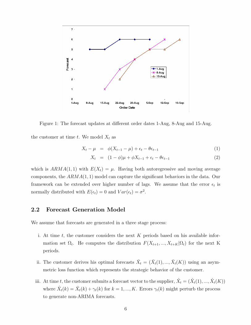
Figure 1: The forecast updates at different order dates 1-Aug, 8-Aug and 15-Aug.

the customer at time t. We model Xt as

Xt − µ = φ(Xt−1 − µ) + εt − θεt−1 (1)

Xt = (1 − φ)µ + φXt−1 + εt − θεt−1 (2)

which is ARMA(1, 1) with E(Xt) = µ. Having both autoregressive and moving average

components, the ARMA(1, 1) model can capture the significant behaviors in the data. Our

framework can be extended over higher number of lags. We assume that the error εt is

normally distributed with E(εt) = 0 and V ar(εt) = σ2.

2.2 Forecast Generation Model

We assume that forecasts are generated in a three stage process:

i. At time t, the customer considers the next K periods based on his available infor-

mation set Ωt. He computes the distribution F (Xt+1, ..., Xt+K |Ωt) for the next K

periods.

ii. The customer derives his optimal forecasts Xt = (Xt(1), ..., Xt(K)) using an asym-

metric loss function which represents the strategic behavior of the customer.

iii. At time t, the customer submits a forecast vector to the supplier, Xt = (Xt(1), ..., Xt(K))

where Xt(k) = Xt(k) + γt(k) for k = 1, ..., K. Errors γt(k) might perturb the process

to generate non-ARIMA forecasts.

6

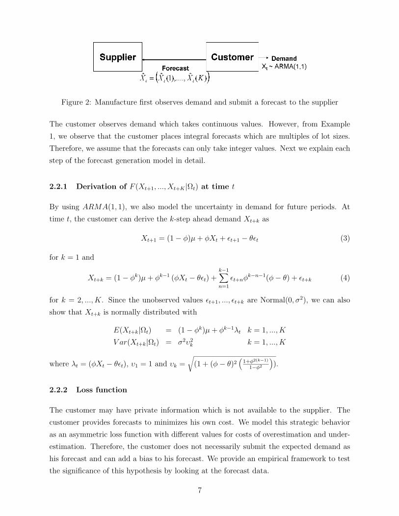
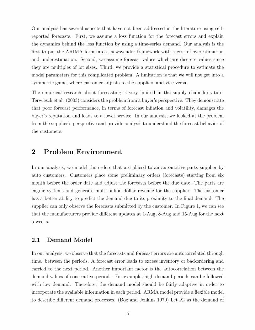
Figure 2: Manufacture first observes demand and submit a forecast to the supplier

The customer observes demand which takes continuous values. However, from Example

1, we observe that the customer places integral forecasts which are multiples of lot sizes.

Therefore, we assume that the forecasts can only take integer values. Next we explain each

step of the forecast generation model in detail.

2.2.1 Derivation of F (Xt+1, ..., Xt+K |Ωt) at time t

By using ARMA(1, 1), we also model the uncertainty in demand for future periods. At

time t, the customer can derive the k-step ahead demand Xt+k as

Xt+1 = (1 − φ)µ + φXt + εt+1 − θεt (3)

for k = 1 and

Xt+k = (1 − φk)µ + φk−1 (φXt − θεt) +k−1∑n=1

εt+nφk−n−1(φ − θ) + εt+k (4)

for k = 2, ..., K. Since the unobserved values εt+1, ..., εt+k are Normal(0, σ2), we can also

show that Xt+k is normally distributed with

E(Xt+k|Ωt) = (1 − φk)µ + φk−1λt k = 1, ..., K

V ar(Xt+k|Ωt) = σ2υ2k k = 1, ..., K

where λt = (φXt − θεt), υ1 = 1 and υk =

√(1 + (φ − θ)2

(1+φ2(k−1)

1−φ2

)).

2.2.2 Loss function

The customer may have private information which is not available to the supplier. The

customer provides forecasts to minimizes his own cost. We model this strategic behavior

as an asymmetric loss function with different values for costs of overestimation and under-

estimation. Therefore, the customer does not necessarily submit the expected demand as

his forecast and can add a bias to his forecast. We provide an empirical framework to test

the significance of this hypothesis by looking at the forecast data.

7

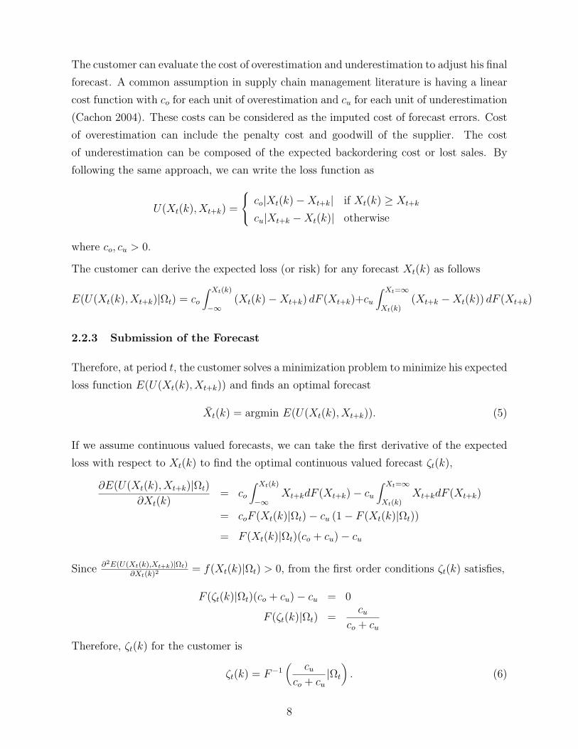
The customer can evaluate the cost of overestimation and underestimation to adjust his final

forecast. A common assumption in supply chain management literature is having a linear

cost function with co for each unit of overestimation and cu for each unit of underestimation

(Cachon 2004). These costs can be considered as the imputed cost of forecast errors. Cost

of overestimation can include the penalty cost and goodwill of the supplier. The cost

of underestimation can be composed of the expected backordering cost or lost sales. By

following the same approach, we can write the loss function as

U(Xt(k), Xt+k) =

co|Xt(k) − Xt+k| if Xt(k) ≥ Xt+k

cu|Xt+k − Xt(k)| otherwise

where co, cu > 0.

The customer can derive the expected loss (or risk) for any forecast Xt(k) as follows

E(U(Xt(k), Xt+k)|Ωt) = co

∫ Xt(k)

−∞(Xt(k) − Xt+k) dF (Xt+k)+cu

∫ Xt=∞

Xt(k)(Xt+k − Xt(k)) dF (Xt+k)

2.2.3 Submission of the Forecast

Therefore, at period t, the customer solves a minimization problem to minimize his expected

loss function E(U(Xt(k), Xt+k)) and finds an optimal forecast

Xt(k) = argmin E(U(Xt(k), Xt+k)). (5)

If we assume continuous valued forecasts, we can take the first derivative of the expected

loss with respect to Xt(k) to find the optimal continuous valued forecast ζt(k),

∂E(U(Xt(k), Xt+k)|Ωt)

∂Xt(k)= co

∫ Xt(k)

−∞Xt+kdF (Xt+k) − cu

∫ Xt=∞

Xt(k)Xt+kdF (Xt+k)

= coF (Xt(k)|Ωt) − cu (1 − F (Xt(k)|Ωt))

= F (Xt(k)|Ωt)(co + cu) − cu

Since ∂2E(U(Xt(k),Xt+k)|Ωt)∂Xt(k)2

= f(Xt(k)|Ωt) > 0, from the first order conditions ζt(k) satisfies,

F (ζt(k)|Ωt)(co + cu) − cu = 0

F (ζt(k)|Ωt) =cu

co + cu

Therefore, ζt(k) for the customer is

ζt(k) = F−1(

cu

co + cu

|Ωt

). (6)

8

Figure 3: The optimal k-step ahead forecasts at time t for µ = 12, σ = 8, φ = 0.7, θ = 0.1,

Xt = 6, εt = 3. The solid line represents an unbiased forecast with cu = co = 1.

When the loss function is symmetric (cu = co), the customer finds the median F−1 (0.5|Ωt)

as the optimal forecast. If the distribution is symmetric, then median is equal to mean

and the customer submits E(Xt+k|Ωt) as the optimal forecast. As can be seen in Figure 3

the customer adds a bias to his forecast when the the loss function is asymmetric. When

cu > co, the customer tends to overestimate his orders and adds a positive bias to his

forecast. When cu < co, it is less costly to underestimate for the customer. In this case

the customer has a negative bias in his forecast. Therefore, asymmetric loss functions can

explain the dynamics behind the bias in the forecasts.

When we assume the the ARMA(1,1) model, the k-period ahead optimal continuous valued

forecast can be derived as :

ζt(k) = (1 − φk)µ + φk−1λt + τσυk k = 1, ..., K

where τ be the z-value of cu

co+cufor standard normal distribution.

In our analysis, we assume that forecasts can only take integer values. Since E(U(Xt(k), Xt(k)))

is convex, the optimal integer valued forecast Xt(k) is

Xt(k) =

bζt(k)c if E(U(bζt(k)c, Xt(k))) < E(U(dζt(k)e, Xt(k)))

dζt(k)e otherwise

where b·c is the floor function and d·e is the ceiling function.

We assume that there might be some errors γt(k) added to the optimal integer valued

forecasts to generate non-ARIMA forecasts. The final forecast is

Xt(k) = Xt(k) + γt(k)

9

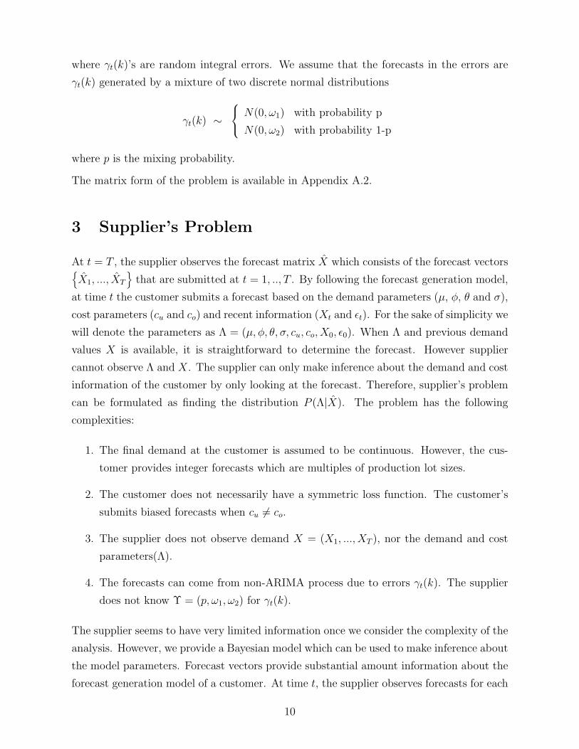
where γt(k)’s are random integral errors. We assume that the forecasts in the errors are

γt(k) generated by a mixture of two discrete normal distributions

γt(k) ∼

N(0, ω1) with probability p

N(0, ω2) with probability 1-p

where p is the mixing probability.

The matrix form of the problem is available in Appendix A.2.

3 Supplier’s Problem

At t = T , the supplier observes the forecast matrix X which consists of the forecast vectorsX1, ..., XT

that are submitted at t = 1, .., T . By following the forecast generation model,

at time t the customer submits a forecast based on the demand parameters (µ, φ, θ and σ),

cost parameters (cu and co) and recent information (Xt and εt). For the sake of simplicity we

will denote the parameters as Λ = (µ, φ, θ, σ, cu, co, X0, ε0). When Λ and previous demand

values X is available, it is straightforward to determine the forecast. However supplier

cannot observe Λ and X. The supplier can only make inference about the demand and cost

information of the customer by only looking at the forecast. Therefore, supplier’s problem

can be formulated as finding the distribution P (Λ|X). The problem has the following

complexities:

1. The final demand at the customer is assumed to be continuous. However, the cus-

tomer provides integer forecasts which are multiples of production lot sizes.

2. The customer does not necessarily have a symmetric loss function. The customer’s

submits biased forecasts when cu 6= co.

3. The supplier does not observe demand X = (X1, ..., XT ), nor the demand and cost

parameters(Λ).

4. The forecasts can come from non-ARIMA process due to errors γt(k). The supplier

does not know Υ = (p, ω1, ω2) for γt(k).

The supplier seems to have very limited information once we consider the complexity of the

analysis. However, we provide a Bayesian model which can be used to make inference about

the model parameters. Forecast vectors provide substantial amount information about the

forecast generation model of a customer. At time t, the supplier observes forecasts for each

10

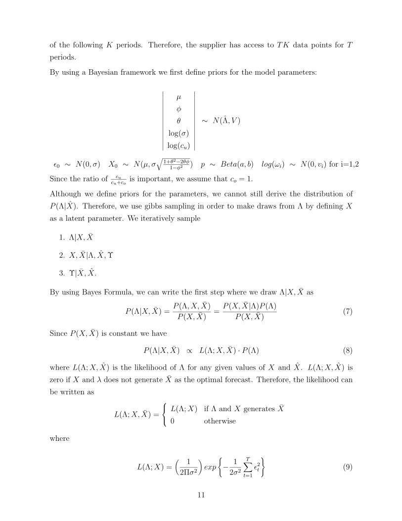
of the following K periods. Therefore, the supplier has access to TK data points for T

periods.

By using a Bayesian framework we first define priors for the model parameters:

∣∣∣∣∣∣∣∣∣∣∣∣∣∣∣

µ

φ

θ

log(σ)

log(cu)

∣∣∣∣∣∣∣∣∣∣∣∣∣∣∣∼ N(Λ, V )

ε0 ∼ N(0, σ) X0 ∼ N(µ, σ√

1+θ2−2θφ1−φ2 ) p ∼ Beta(a, b) log(ωi) ∼ N(0, vi) for i=1,2

Since the ratio of cu

cu+cois important, we assume that co = 1.

Although we define priors for the parameters, we cannot still derive the distribution of

P (Λ|X). Therefore, we use gibbs sampling in order to make draws from Λ by defining X

as a latent parameter. We iteratively sample

1. Λ|X, X

2. X, X|Λ, X, Υ

3. Υ|X, X.

By using Bayes Formula, we can write the first step where we draw Λ|X, X as

P (Λ|X, X) =P (Λ, X, X)

P (X, X)=

P (X, X|Λ)P (Λ)

P (X, X)(7)

Since P (X, X) is constant we have

P (Λ|X, X) ∝ L(Λ; X, X) · P (Λ) (8)

where L(Λ; X, X) is the likelihood of Λ for any given values of X and X. L(Λ; X, X) is

zero if X and λ does not generate X as the optimal forecast. Therefore, the likelihood can

be written as

L(Λ; X, X) =

L(Λ; X) if Λ and X generates X

0 otherwise

where

L(Λ; X) =(

1

2Πσ2

)exp

− 1

2σ2

T∑t=1

ε2t

(9)

11

4 Estimation

The supplier wants to derive the distribution of parameters given the forecast matrix,

P (Λ|X). Our sampler is a modified slice sampler with rejection. The general slice sam-

pling algorithm (Neal 2003) is constructed using the principle that one can sample from a

distribution by sampling uniformly from the region under the plot of its density function.

4.1 Mechanism of the Slice Sampler

Assume that we want to sample from a distribution for a variable x ∈ Rn, which has

density function f(x). We can introduce an auxiliary variable real variable, y and define

joint distribution function p(x, y) of x and y which is uniformly distributed over the region

S = (x, y) : 0 < y ≤ f(x). S is the area under f(x). Let Z =∫

f(x), then we have

p(x, y) =

1/Z, if 0 < y < f(x)

0, otherwise

The marginal density for x is

p(x) =∫ f(x)

01/Zdy = f(x)/Z (10)

We can sample jointly for (x, y) and keep x values to replicate f(x).

4.2 Our Sampler for Estimation

We first find an initial set of Λ, X, X and υ which can generate the forecast matrix X. We

then iteratively sample

1. Λ|X, X

2. X, X|Λ, X, Υ

3. Υ|X, X.

Our sampler works as follows:

Iteration 0 (Initialization):

12

1. Draw µ(0),φ(0), θ(0), σ(0), c(0)u , ε

(0)0 and X

(0)0 from the prior distributions.

∣∣∣∣∣∣∣∣∣∣∣∣∣∣∣

µ(0)

φ(0)

θ(0)

log(σ(0))

log(c(0)u )

∣∣∣∣∣∣∣∣∣∣∣∣∣∣∣∼ N(Λ, V )

ε(0)0 ∼ N(0, σ) X

(0)0 ∼ N(µ, σ

√1+θ2−2θφ

1−φ2 )

where −1 ≤ φ(0) ≤ 1 and −1 ≤ θ(0) ≤ 1.

2. Draw ε(0) =ε(0)1 , ..., ε

(0)T

from N(0, Iσ2). Compute X(0) and optimal X(0).

X(0)t = (1 − φ(0))µ(0) + φ(0)X

(0)t−1 + ε

(0)t − θε

(0)t−1

and

Xt(k)(0) = argmin E(U(Xt(k), Xt+k)). (11)

for t = 1, ..., T and k = 1, ..., K.

3. Draw p(0), ω(0)1 and ω

(0)2 from the priors

p(0) ∼ Beta(a, b) log(ω(0)1 ) ∼ N(0, v1) log(ω

(0)2 ) ∼ N(0, v2)

Repeat the following for a specified number (I) of iterations. (for i=1,...,I)

Iteration i:

1. In this step, we generate Λi|X(i−1), X(i−1). So we draw

• µ(i)|φ(i−1), θ(i−1), c(i−1)u , σ(i−1), ε

(i−1)0 , X

(i−1)0 , X(i−1), X(i−1)

• φ(i)|µ(i), θ(i−1), c(i−1)u , σ(i−1), ε

(i−1)0 , X

(i−1)0 , X(i−1), X(i−1)

• θ(i)|µ(i), φ(i), c(i−1)u , σ(i−1), ε

(i−1)0 , X

(i−1)0 , X(i−1), X(i−1)

• c(i)u |µ(i), φ(i), θ(i), σ(i−1), ε

(i−1)0 , X

(i−1)0 , X(i−1), X(i−1)

• σ(i)|µ(i), φ(i), θ(i), c(i)u ε

(i−1)0 , X

(i−1)0 , X(i−1), X(i−1)

• ε(i)0 |µ(i), φ(i), θ(i), c(i)

u , σ(i)X(i−1)0 , X(i−1), X(i−1)

• X(i)0 |µ(i), φ(i), θ(i), c(i)

u , σ(i), ε(i)0 , X(i−1), X(i−1)

13

by using a sequential slice sampler. Here, we show how we draw θ(i). The same

analysis is repeated for all the above parameters in the given order.

(a) Since we always guarantee to have feasibility of X in each step, we can compute

the likelihood

L(i−1)θ = L(Λ; X(i−1), X(i−1))

= L(Λ; X(i−1))

= P (X(i−1)1 , ..., X

(i−1)T |µ(i), φ(i), θ(i−1), c(i−1)

u ε(i−1)0 , X

(i−1)0 )

This is our vertical slice.

(b) Draw a random variable uθ from Uniform(0, L(i−1)θ ). This is our horizontal slice.

(c) While true,

i. Draw θ(i) from the prior distribution θ(i)|µ(i), φ(i), c(i−1)u , σ(i−1). We have

Λ′ =

∣∣∣∣∣∣∣∣∣∣∣∣∣∣∣

µ(i)

φ(i)

θ(i)

log(σ(i−1))

log(c(i−1)u )

∣∣∣∣∣∣∣∣∣∣∣∣∣∣∣∼ N(Λ, V )

From proposition 1, we have the conditional truncated distribution

θ(i)|µ(i), φ(i), c(i−1)u , σ(i−1) ∼ N(Λ3+V3,−3V

−1−3,−3(Λ

′−3−Λ−3), Λ3,3−Λ3,−3Λ

−1−3,−3Λ−3,3)

for −1 ≤ θ(i) ≤ 1.

ii. Check the feasibility of the draw 1. If the solution is not feasible go to

Step (i) and make another draw for θ(i). Otherwise, find the likelihood

L(i)θ = P (X

(i−1)1 , ..., X

(i−1)T |µ(i), φ(i), θ(i−1), c(i−1)

u , ε(i−1)0 , X

(i−1)0 ). If L

(i)θ > uθ,

then keep θ(i) and repeat the same analysis for the next parameter(c(i)u in

this case).

2. In this step, we generate the X(i), X(i)|Λ(i), Υ(i), X. This can be done in two ways:

(a) We can draw Xt|Λ(i), X(i)−t by using a sequential slice sampler for t = 1, ..., T

where

X(i)−t =

X

(i)1 , ..., X

(i)t−1, X

(i−1)t+1 , ..., X

(i−1)T

1For K=1, the parameters are always feasible. For K > 1 we need the feasibility which means that

X(i−1) and Λ(i) generates the optimal forecast X

14

i. We compute the likelihood L(i−1)X = P (γ(i−1); υ(i−1)) where

γt(k)(i−1) = Xt(k)(i−1) − Xt(k)(i−1)

for t = 1, ..., T and k = 1, ..., K.

This is our vertical slice.

ii. Draw a random variable uX from Uniform(0, L(i)X ). This is our horizontal

slice.

iii. While true,

A. We can show that Xt|Λ(i), X(i)−t follows a truncated normal distribution.

Draw Xt from the truncated normal distribution.

B. Compute the likelihood L(i)X = P (γ(i); υ(i−1)). If L

(i)X > uX , then keep

X(i)t otherwise make another draw for Xt.

(b) This can also be done by drawing ε ∼ N(0, σ2I) by using a slice sampler. In

this case we draw ε together and compute the likelihood.

3. In this step, we generate Υ(i)|X(i), X. We first compute γ(i) as follows

γt(k)(i−1) = Xt(k)(i−1) − Xt(k)(i−1)

for t = 1, ..., T and k = 1, ..., K.

So we draw

• p(i)|ω(i−1)1 , ω

(i−1)2 , γ(i)

• ω(i)1 |p(i), ω

(i−1)2 , γ(i)

• ω(i)2 |p(i), ω

(i)1 , γ(i)

by using a sequential slice sampler. Here, we show how we draw p(i). The same

analysis is repeated for all the above parameters in the given order.

(a) We can compute the likelihood

L(i−1)p = P (γ(i)|Υ(i−1))

This is our vertical slice.

(b) Draw a random variable up from Uniform(0, L(i−1)p ). This is our horizontal slice.

(c) While true,

15

i. Draw p(i) from the prior Beta(a, b).

ii. Find the likelihood L(i)p = P (γ(i)|p(i), ω

(i−1)1 , ω

(i−1)2 ). If L(i−1)

p > up, then keep

p(i) and repeat the same analysis for the next parameter(ω(i)1 in this case).

Otherwise make another draw from the prior for p(i).

We also use shrinkage algorithm (Neal 2003) to improve the draws for the slice sampler. By

doing that we decrease the number of rejected draws to find a feasible set of parameters.

4.3 Example

We use the customer forecasts in Example 1 to show the results of estimation. In Example

1, we only have forecasts for three weeks. By adding the forecasts for the following 17

weeks, we have the forecast vector X in Figure 4a. X provides K = 5 weeks forecasts in

T = 20 weeks. We assume the following priors for estimation:

µ ∼ N(10, 5) φ ∼ N(0, 0.5) θ ∼ N(0, 0.5)

σ ∼ IG(2.5, 10) log(cu) ∼ N(0, 1)

ε ∼ N(0, σ) X0 ∼ N(µ, σ√

1+θ2−2θφ1−φ2 )

We run our sampler for 40, 000 iterations to estimate the posterior distributions of each

parameters. We discard the first 3, 000 observations as the warmup period. The results

are available in Figure 4. Some of the inferences that we can make from the posterior

distributions are as follows:

• We can see that the autoregressive parameter (φ) has a 95% confidence interval of

(0.59, 0.64). Therefore, there is a significant effect of the previous demand observation

on the current demand. However, for θ, the posterior centers around 0. We cannot

reject the hypothesis that θ = 0. This means that error terms are not autocorrelated,

however there is strong autocorrelation between the consecutive demand values.

• When we test the hypothesis that cu > co = 1, we cannot reject it with α = 95%.

This means that there is significant evidence from the data that the customer adds a

positive bias to his forecasts.

• When we look at σ, we can see that there is high uncertainty at the customer. The

high variance is an important factor that causes errors in the forecasts. However, σ

by itself does not explain the forecast errors. As we discuss above, the customer adds

a bias to forecasts due to his asymmetric loss function.

16

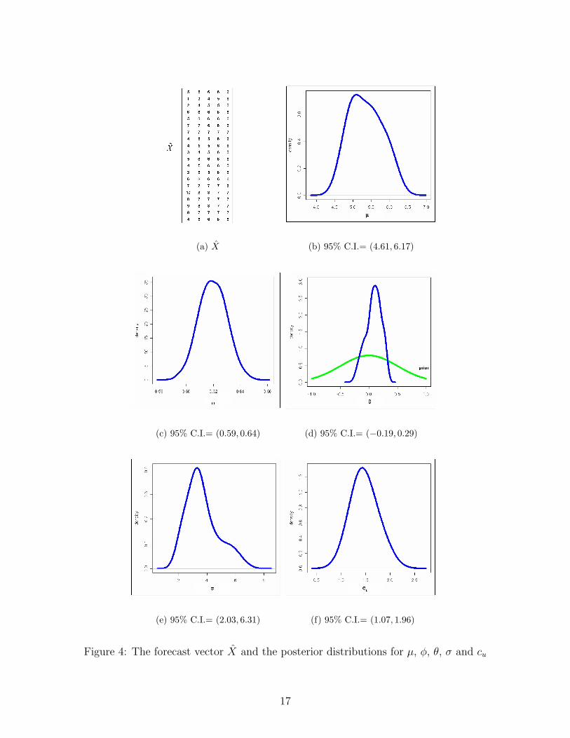
(a) X (b) 95% C.I.= (4.61, 6.17)

(c) 95% C.I.= (0.59, 0.64) (d) 95% C.I.= (−0.19, 0.29)

(e) 95% C.I.= (2.03, 6.31) (f) 95% C.I.= (1.07, 1.96)

Figure 4: The forecast vector X and the posterior distributions for µ, φ, θ, σ and cu

17

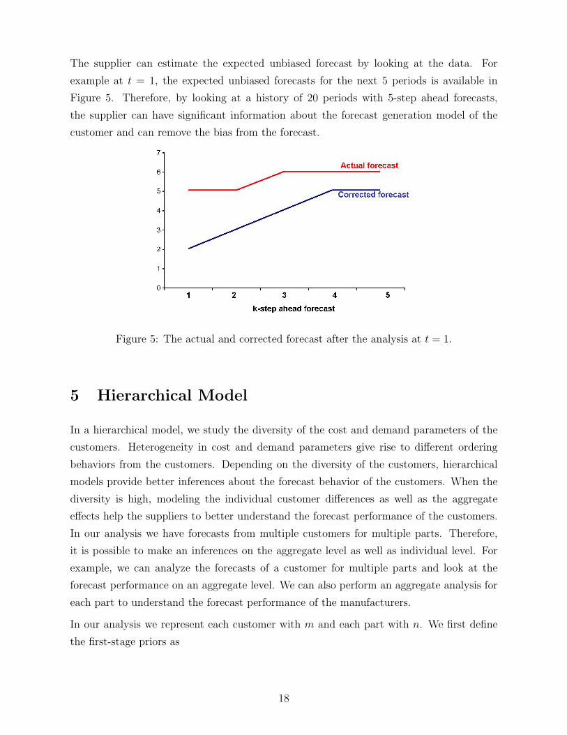
The supplier can estimate the expected unbiased forecast by looking at the data. For

example at t = 1, the expected unbiased forecasts for the next 5 periods is available in

Figure 5. Therefore, by looking at a history of 20 periods with 5-step ahead forecasts,

the supplier can have significant information about the forecast generation model of the

customer and can remove the bias from the forecast.

Figure 5: The actual and corrected forecast after the analysis at t = 1.

5 Hierarchical Model

In a hierarchical model, we study the diversity of the cost and demand parameters of the

customers. Heterogeneity in cost and demand parameters give rise to different ordering

behaviors from the customers. Depending on the diversity of the customers, hierarchical

models provide better inferences about the forecast behavior of the customers. When the

diversity is high, modeling the individual customer differences as well as the aggregate

effects help the suppliers to better understand the forecast performance of the customers.

In our analysis we have forecasts from multiple customers for multiple parts. Therefore,

it is possible to make an inferences on the aggregate level as well as individual level. For

example, we can analyze the forecasts of a customer for multiple parts and look at the

forecast performance on an aggregate level. We can also perform an aggregate analysis for

each part to understand the forecast performance of the manufacturers.

In our analysis we represent each customer with m and each part with n. We first define

the first-stage priors as

18

Λ′mn =

∣∣∣∣∣∣∣∣∣∣∣∣∣∣∣

µmn

φmn

θmn

log(σ)mn

log(cu)mn

∣∣∣∣∣∣∣∣∣∣∣∣∣∣∣∼ N(Λ, V )

The second stage priors are

V ∼ Inverted Wishart(ν0, S0)

Λ ∼ N(0, Λ0)

In order to have a full rank ν0 > 5 which is the number of parameters. Assume that we run

an analysis over M different customers for a part. So we can drop n from the subscript in

this case, we have

P (V ) ∝ |V |−ν0−6

2 etr(−1

2S0V

−1)

The posterior from the data is

P (V |Λ′1, ..., Λ

′M ∝ |V |−

M+ν0−6

2 etr(−1

2(S0 + S+)V −1

)= Inverted Wishart(ν0 + M, S0 + S)

where S =∑M

m=1(Λ′m − Λ′)(Λ′

m − Λ′)T .

The posterior for Λ from the data is

P (Λ|V, Λ′1, ..., Λ

′M ∝ exp

(1

2(Λ − ΛM)T V −1

M (Λ − ΛM))

= N(Λ|ΛM , VM)

where

VM = Λ−10 + MV −1

ΛM = V −1M MV −1Λ′

In order to predict the parameters, in iteration i we sequentially draw

1. For customers m = 1, ...,M , we draw Λ′(i)m |Λ′(i−1) by using the sampler in section 4.2.

2. We draw V (i)|Λ′(i)1 , ..., Λ

′(i)M from the posterior distribution N(Λ|Λ(i)

M , V(i)M ).

3. We draw Λ(i)|V (i), Λ′(i)1 , ..., Λ

′(i)M from the posterior distribution Inverted Wishart(ν0+

M, S0 + S(i)).

19

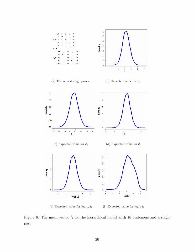
(a) The second stage priors (b) Expected value for µi

(c) Expected value for φi (d) Expected value for θi

(e) Expected value for log(cu)i (f) Expected value for log(σ)i

Figure 6: The mean vector Λ for the hierarchical model with 16 customers and a single

part

20

5.1 Example

In Figure 6, we provide the estimates for the mean level Λ of the model parameters. We

analyze a part with 16 customers. During our analysis, we observe that for most of the

customers, our model represents a good fit and we do not observe too many errors in the

forecasts. For only 3 customers, we observe that the forecasts are generated from a different

process. Therefore, the estimates for the model parameters were not significant for those

customers.

From 6, we have the following observations:

1. We can see that φ and θ tends to be greater than zero. This means that the autocor-

relations between the forecasts and the errors of the consecutive periods tend to be

positive.

2. The log value of cost of underestimation is very close to normal distribution with a

mean value slightly less than zero. This means that underestimation is also a common

behavior among the customers. This also shows that log transformation is necessary

while analyzing the cost of overestimation and underestimation. At the individual

level, we get more significant results for the customers where we cannot reject the

hypothesis for customers over- or underestimating their orders.

3. The standard deviation of the demand tends to be small for some of the customers.

For those customers, we can argue that the forecast errors are mostly due to the cost

structure of the customer rather than the uncertainty in usage.

6 Conclusion and Future Research

We have used a time-series framework to model the evolution of forecast vectors. In our

data, we observe that customers consistently overestimate or underestimate their orders.

The goal of our analysis was to develop a framework to test the significance of strategic

behavior. By using asymmetric loss functions, we explain the dynamics behind the bias in

customer’s forecasts. We present an estimation procedure which has high predictive power

to understand the cost and demand structure of a customer from his forecasts.

Our hierarchical model can be extended in order to include individual parameters for each

customer and part. We can also include exogenous parameters in order to test their ef-

fect on the forecast performance of the customers. The hierarchical models for multiple

21

customers and parents are ideal for gibbs sampling methods, where we sequentially draw

individual parameters by conditioning on the other parameters. We mainly use the pos-

terior distributions or slice sampling to draw the parameters. Other MCMC methods can

also be considered for the analysis. The main advantage of the slice sampler is we do not

need to tune the parameters and provide a proposal density.

We show that the customers add bias to their forecast due to their cost and demand

structure. Therefore, it is critical for a supplier to create unbiased forecasts from the

reported forecasts. Our analysis helps us understand which factors influence the forecast

behavior of a manufacturer. A high σ for a customer shows that there is high uncertainty

in the usage. A high cu signals high cost of stockouts at the customer. We can also make

inferences on the aggregate level. If we detect a common poor forecast performance across

the customers, there might be problems with shipping of the product which creates artificial

spikes in the forecasts. Hierarchical model helps us understand how much of the errors can

be explained from the individual and aggregate demand and cost structure.

The customer demand can follow non-ARMA processes. In this case we observe high ω1 or

ω2 values which show that the forecasts from the model do not fit the reported forecasts

very well. Therefore, some other demand models can be considered for the non-ARMA

customers. Our analysis can be extended to models with more components to capture

these complexities. Possible such extensions are adding seasonality, production plans and

nonlinear loss functions.

References

[1] N. Altintas and M. Trick. A data mining approach to forecast behavior of manufac-

turers in automotive industry. Working paper, Tepper School of Business, Carnegie

Mellon University, Pittsburgh, PA, 2004.

[2] Y. Aviv. The effect of collaborative forecasting on supply chain performance. Man-

agement Science, 47:1326–1343, 2001.

[3] Y. Aviv. Gaining benefits from joint forecasting and replenishment processes: The

case of auto-correlated demand. Manufacturing and Service Operations Management,

4:55–74, 2002.

[4] Y. Aviv. A time-series framework for supply-chain inventory management. Operations

Research, 51(2):210–227, 2003.

22

[5] K. S. Azoury. Bayes solution to dynamic inventory models under unknown demand

distribution. Management Science, 31:1150–1160, 1985.

[6] Roy Batchelor and Pami Dua. Forecaster diversity and the benefits of combining

forecasts. Management Science, 41(1):68–75, 1995.

[7] G. E. P. Box and G. M. Jenkins. Time Series Analysis: Forecasting and Control. San

Francisco, Holden-Day, 1970.

[8] G. Cachon and S. Netessine. Game theory in supply chain analysis. In S. D. Wu

D. Simchi-Levi and Z. Shen, editors, Handbook of Quantitative Supply Chain Analysis:

Modeling in the eBusiness Era. Kluwer, 2004.

[9] J. Geweke and C. Whiteman. Bayesian forecasting. In C.W.J. Granger G. Elliott and

A. Timmermann, editors, The Handbook of Economic Forecasting. Elsevier, 2006.

[10] S. C. Graves. A tactical planning model for a job shop. Operations Research, 34:522–

533, 1986a.

[11] S. C. Graves, D. B. Kletter, and W. B. Hetzel. A dynamic model for requirements

planning with application to supply chain optimization. Operations Research, 46:S35–

S49, 1998.

[12] S. C. Graves, D. B. Kletter, and W. B. Hetzel. A single-item inventory model for a

non-stationary demand process. Manufacturing and Service Operations Management,

1(1):50–61, 1999.

[13] S. C. Graves, H.C. Meal, S. Dasu, and Y. Qiu. Two stage production planning in a dy-

namic environment. In S. Axsater, C. Schneeweiss, and E.Silver, editors, Multi-Stage

Production Planning and Control: Lecture Notes in Economics and Mathematical Sys-

tems, pages 9–43. Springer-Verlag, Berlin, 1986b.

[14] R. Gullu. On the value of information in dynamic production/inventory problems

under forecast evolution. Naval Research Logistics, 43:289–303, 1986.

[15] D. C. Heath and P. Jackson. Modeling the evolution of demand forecasts with appli-

cation to safety stock analysis in production/distribution systems. IIE Transactions,

26:17–30, 1994.

[16] R. A. Johnson and D. W. Wichern. Applied Multivariate Statistics. Prentice Hall,

1992.

23

[17] M. A. Lariviere and E. L. Porteus. Stalking information: Bayesian inventory manage-

ment with unobserved lost sales. Management Science, 45:346–363, 1999.

[18] R. M. Neal. Slice sampling. The Annals of Statistics, 31(3):705–767, 2003.

[19] H. Scarf. Bayes solutions of the statistical inventory problem. Annals of Mathematical

Statistics, 30:490–508, 1959.

[20] C. Terwiesch, J. Z. Ren, T. H. Ho, and M. Cohen. An empirical analysis of forecast

sharing in the semiconductor equipment industry. Working paper, Wharton Business

School, University of Pennsylvania, Philadelphia, PA, 2003.

[21] B. Toktay and L. M. Wein. Analysis of a forecasting-production-inventory system with

stationary demand. Management Science, 47:1268–1281, 2001.

24

A Appendix

A.1 The conditional distribution of X1

Proposition 1 Let X be distributed as N(µ, Σ) and

X =

∣∣∣∣∣∣ X1

X2

∣∣∣∣∣∣ Σ =

∣∣∣∣∣∣ Σ11 Σ12

Σ21 Σ22

∣∣∣∣∣∣ µ =

∣∣∣∣∣∣ µ1

µ2

∣∣∣∣∣∣Then the conditional distribution of X1, given X2 is N(µ1 + Σ12Σ

−122 (X2 − µ2), Σ11 −

Σ12Σ−122 Σ21).

Proof: Available in Johnson and Wichern (1992).

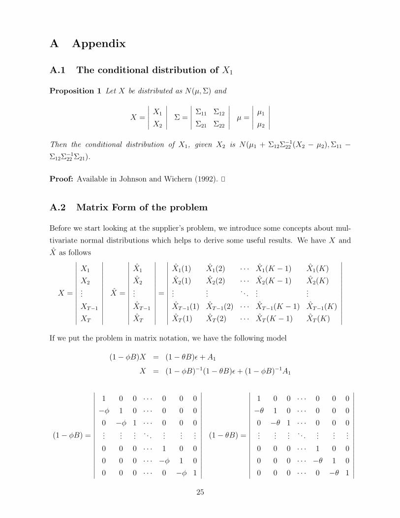
A.2 Matrix Form of the problem

Before we start looking at the supplier’s problem, we introduce some concepts about mul-

tivariate normal distributions which helps to derive some useful results. We have X and

X as follows

X =

∣∣∣∣∣∣∣∣∣∣∣∣∣∣∣∣

X1

X2

...

XT−1

XT

∣∣∣∣∣∣∣∣∣∣∣∣∣∣∣∣X =

∣∣∣∣∣∣∣∣∣∣∣∣∣∣∣∣

X1

X2

...

XT−1

XT

∣∣∣∣∣∣∣∣∣∣∣∣∣∣∣∣=

∣∣∣∣∣∣∣∣∣∣∣∣∣∣∣∣

X1(1) X1(2) · · · X1(K − 1) X1(K)

X2(1) X2(2) · · · X2(K − 1) X2(K)...

.... . .

......

XT−1(1) XT−1(2) · · · XT−1(K − 1) XT−1(K)

XT (1) XT (2) · · · XT (K − 1) XT (K)

∣∣∣∣∣∣∣∣∣∣∣∣∣∣∣∣If we put the problem in matrix notation, we have the following model

(1 − φB)X = (1 − θB)ε + A1

X = (1 − φB)−1(1 − θB)ε + (1 − φB)−1A1

(1 − φB) =

∣∣∣∣∣∣∣∣∣∣∣∣∣∣∣∣∣∣∣∣∣∣

1 0 0 · · · 0 0 0

−φ 1 0 · · · 0 0 0

0 −φ 1 · · · 0 0 0...

......

. . ....

......

0 0 0 · · · 1 0 0

0 0 0 · · · −φ 1 0

0 0 0 · · · 0 −φ 1

∣∣∣∣∣∣∣∣∣∣∣∣∣∣∣∣∣∣∣∣∣∣

(1 − θB) =

∣∣∣∣∣∣∣∣∣∣∣∣∣∣∣∣∣∣∣∣∣∣

1 0 0 · · · 0 0 0

−θ 1 0 · · · 0 0 0

0 −θ 1 · · · 0 0 0...

......

. . ....

......

0 0 0 · · · 1 0 0

0 0 0 · · · −θ 1 0

0 0 0 · · · 0 −θ 1

∣∣∣∣∣∣∣∣∣∣∣∣∣∣∣∣∣∣∣∣∣∣25

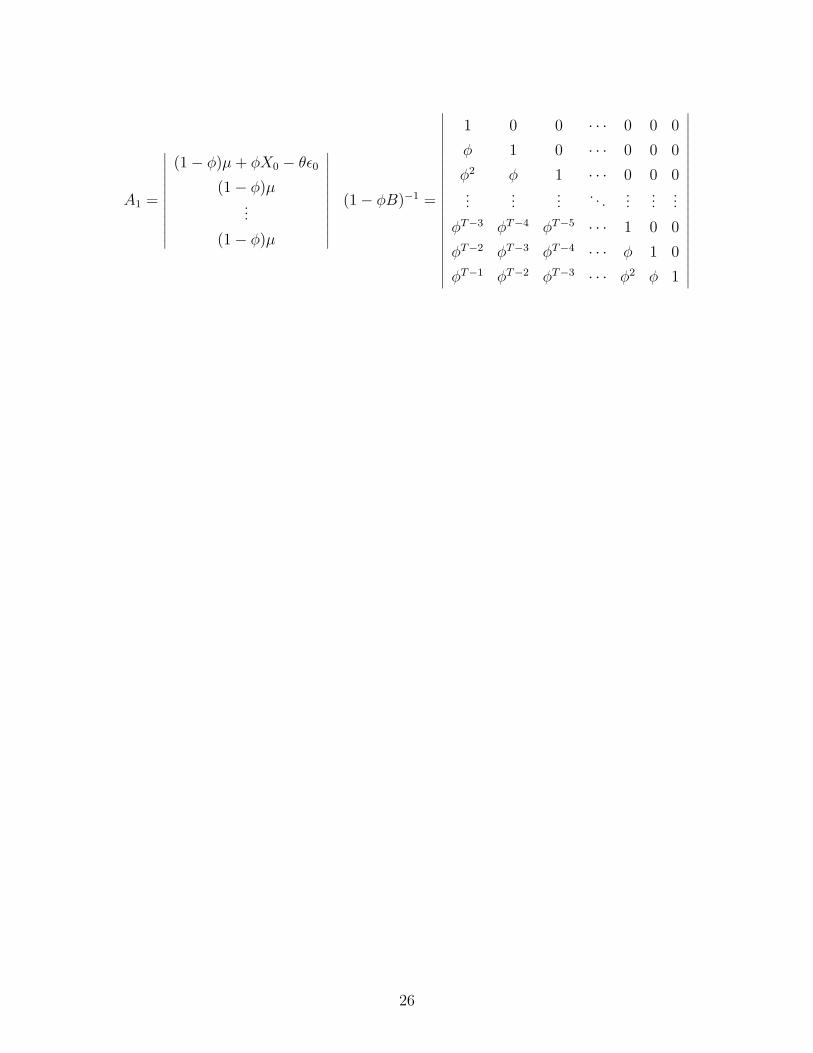
A1 =

∣∣∣∣∣∣∣∣∣∣∣∣

(1 − φ)µ + φX0 − θε0

(1 − φ)µ...

(1 − φ)µ

∣∣∣∣∣∣∣∣∣∣∣∣(1 − φB)−1 =

∣∣∣∣∣∣∣∣∣∣∣∣∣∣∣∣∣∣∣∣∣∣

1 0 0 · · · 0 0 0

φ 1 0 · · · 0 0 0

φ2 φ 1 · · · 0 0 0...

......

. . ....

......

φT−3 φT−4 φT−5 · · · 1 0 0

φT−2 φT−3 φT−4 · · · φ 1 0

φT−1 φT−2 φT−3 · · · φ2 φ 1

∣∣∣∣∣∣∣∣∣∣∣∣∣∣∣∣∣∣∣∣∣∣

26