author's personal copy - university of...
TRANSCRIPT

This article appeared in a journal published by Elsevier. The attachedcopy is furnished to the author for internal non-commercial researchand education use, including for instruction at the authors institution
and sharing with colleagues.
Other uses, including reproduction and distribution, or selling orlicensing copies, or posting to personal, institutional or third party
websites are prohibited.
In most cases authors are permitted to post their version of thearticle (e.g. in Word or Tex form) to their personal website orinstitutional repository. Authors requiring further information
regarding Elsevier’s archiving and manuscript policies areencouraged to visit:
http://www.elsevier.com/authorsrights

Author's personal copy
What do consumers believe about future gasoline prices?
Soren T. Anderson a, Ryan Kellogg b, James M. Sallee c,n
a Michigan State University, NBER, United Statesb University of Michigan, NBER, United Statesc University of Chicago, NBER, United States
a r t i c l e i n f o
Article history:Received 26 November 2012Available online 27 July 2013
Keywords:Gasoline pricesConsumer beliefsAutomobile demandEnergy efficiency
a b s t r a c t
A full understanding of how gasoline prices affect consumer behavior frequently requiresinformation on how consumers forecast future gasoline prices. We provide the firstevidence on the nature of these forecasts by analyzing two decades of data on gasolineprice expectations from the Michigan Survey of Consumers. We find that averageconsumer beliefs are typically indistinguishable from a no-change forecast, justifying anassumption commonly made in the literature on consumer valuation of energy efficiency.We also provide evidence on circumstances in which consumer forecasts are likely todeviate from no-change and on significant cross-consumer forecast heterogeneity.
& 2013 Elsevier Inc. All rights reserved.
1. Introduction
The price of gasoline is important for the economy and for economic research. Gas prices are particularly salient toconsumers, and motor fuels account for 5% of all consumer expenditures. Moreover, oil price shocks are strongly correlated withrecessions, even more than gasoline's expenditure share would explain (Hamilton, 2008). Consumer reactions to gasoline priceshave been used to study a broad array of economic phenomena, ranging from the demand for automobiles (Busse et al., 2013; Liet al., 2009; Allcott, 2012; Gillingham, 2011; Linn and Klier, 2010) and driving choices (Small and Van Dender, 2007; Knittel andSandler, 2012; Davis and Kilian, 2011; Li et al., 2012), to the consumption of leisure (West and Williams, 2007), search behavior(Lewis and Marvel, 2011), and mental accounting (Hastings and Shapiro, 2011).
Understanding how consumers respond to gasoline prices today requires information about what consumers believeabout future gasoline prices. For example, if an increase in today's price causes consumers to expect an even higher pricetomorrow, the effect of current price shocks on the macroeconomy could be amplified, perhaps by enough to explain thestronger-than-expected correlation between current prices and economic growth.
Unfortunately, little to no evidence exists regarding consumers' beliefs about future gasoline prices. What does theaverage consumer believe the future price of gasoline will be, and how does this belief vary with the current price? Howvaried are beliefs across individuals? Are consumers' beliefs reasonable? Do beliefs respond differently to different types ofgasoline price shocks? How should researchers model consumer beliefs? In the absence of direct evidence, prior researchhas been left to make assumptions that are often guided by convenience. In this paper, we take first steps toward answeringthese questions by analyzing data from a high-quality survey that directly elicits consumer beliefs.
Contents lists available at ScienceDirect
journal homepage: www.elsevier.com/locate/jeem
Journal ofEnvironmental Economics and Management
0095-0696/$ - see front matter & 2013 Elsevier Inc. All rights reserved.http://dx.doi.org/10.1016/j.jeem.2013.07.002
n Corresponding author. Fax: +1 773 702 2286.E-mail addresses: [email protected] (S.T. Anderson), [email protected] (R. Kellogg), [email protected] (J.M. Sallee).URLS: http://www.msu.edu/�sta (S.T. Anderson), http://www-personal.umich.edu/�kelloggr (R. Kellogg),
http://home.uchicago.edu/�sallee (J.M. Sallee).
Journal of Environmental Economics and Management 66 (2013) 383–403
Author's personal copy
When consumers buy energy-using durable goods, they must forecast the future price of energy to determine theirwillingness to pay for energy efficiency. In turn, research that attempts to estimate or control statistically for consumers'valuation of energy efficiency must explicitly model consumers' beliefs about future energy prices and may draw biasedinferences if these beliefs are mis-specified. This issue is most relevant for studies using identification strategies that rely ontime-series variation in energy prices to identify demand—a strategy that is particularly common in automobile research(Kahn, 1986; Goldberg, 1998; Kilian and Sims, 2006; Li et al., 2009; Allcott and Wozny, 2011; Bento et al., 2012; Klier andLinn, 2010; Sallee et al., 2009; Whitefoot et al., 2011; Langer and Miller, 2011; Linn and Klier, 2010; Busse et al., 2013). Thesestudies frequently assume that consumers adopt no-change forecasts for future gasoline prices in real terms; that is, theyassume that the expected future price is the current price.1 If consumer beliefs deviate significantly from this assumption,then researchers may under-estimate or over-estimate consumers' valuation of fuel economy (and other importantattributes) depending on the direction of the deviation.2
In lieu of direct evidence, there is perhaps little reason to believe that consumer expectations will align convenientlywith the no-change hypothesis favored by applied researchers. Future crude oil and gasoline prices are notoriouslydifficult to predict, and there is substantial controversy among academic and industry experts about what the future priceof oil will be and how best to predict future prices (Hamilton, 2009; Alquist and Kilian, 2010; Alquist et al., 2013). Themain goal of our paper is therefore to test directly whether consumers forecast the future price of gasoline to equal thecurrent price.
We conduct our analysis using high-frequency data on consumer beliefs about future gasoline prices from the MichiganSurvey of Consumers (MSC). Every month, the MSC asks a nationally representative sample of about 500 respondents toreport their beliefs about the current state of the economy and to forecast several economic variables. Since 1993, the MSChas regularly asked respondents to report whether they think gasoline prices will be higher or lower (or the same) in fiveyear's time and then to forecast the exact price change. To the best of our knowledge, we (along with Richard Curtin, ourcollaborator on a related paper (Anderson et al., 2011)) are the first researchers to use this unique cache of information ongasoline price expectations, and very little existing work directly measures consumer beliefs about future energy prices inany context.3
Our analysis indicates that in normal economic climates the average consumer expects the future real price of gasoline toequal the current price. That is, we generally cannot reject the hypothesis, commonly assumed in the automobile demandliterature, that the average consumer's forecast of future gasoline prices moves one-for-one with changes in the currentprice. While a no-change gasoline price forecast is obviously not perfect, we believe it is a good benchmark for determiningwhether consumer forecasts are reasonable.4
We do identify some specific settings in which the average consumer's forecast deviates from no-change. The first suchcase is the 2008 financial crisis, during which consumers predicted that gasoline prices would rebound following their sharpdecline. In a companion paper, Anderson et al. (2011), we show that this prediction turned out to be prescient. The secondcase deals with state-specific price shocks, such as those that might arise from local refinery outages, which tend to be shortlived and for which a no-change forecast is therefore clearly inaccurate. We find that consumer forecasts do change less thanone-for-one with state-specific gasoline price movements, but they nevertheless predict more persistence in state-specificshocks than is actually present in the historical data.
Two recent papers, Davis and Kilian (2011) and Li et al. (2012), find that gasoline consumption is much more responsiveto changes in gasoline taxes than to changes in pre-tax gasoline prices. One explanation for this result, emphasized by bothpapers, is that consumers might perceive changes in gasoline tax policy to be more persistent than price fluctuations causedby shifts in supply and demand. We use our data to directly test this hypothesis, but we find no evidence that consumerforecasts respond more strongly to tax changes than to pre-tax price changes.
We also find substantial heterogeneity in forecasts across consumers. In our sample, the standard deviation in the priceforecast across respondents each month averages 62 cents (in 2010 dollars). Using a simple simulation, we find that thisheterogeneity may generate as much variation in consumers' willingness to pay for fuel economy as is generated byheterogeneity across consumers in vehicle miles traveled or discount rates. We also find that the degree of heterogeneity inconsumers' forecasts co-varies with gasoline prices and that, whenwe study consumers who are surveyed twice (six monthsapart), this heterogeneity is mostly accounted for by individual fixed effects. We believe these results will be valuable for a
1 Equivalently, consumers are assumed to believe that gasoline prices follow a martingale process. Throughout the paper, we use the “no-change”terminology as it accords with the literature on oil price forecasting (see for example Alquist et al., 2013). We do not use the term “randomwalk” because arandom walk process further implies that the price innovations are iid.
2 This issue is a specific instance of the broader empirical problem, discussed by Manski (2004), that preferences and expectations are generally notboth identified from choice data alone.
3 One recent exception is Allcott (2012), which estimates automobile demand using a specially designed survey instrument that asks consumers toreport (among other things) their beliefs about future gasoline prices in real terms. We compare our results to Allcott's below.
4 A no-change forecast for crude oil is theoretically sensible because rapidly rising or falling prices would induce storage and extraction arbitrage(Hamilton, 2009). In addition, no-change forecasts predict future crude oil prices as well as or better than forecasts based on futures markets and surveys ofexperts (Alquist and Kilian, 2010; Alquist et al., 2013). This argument is based on the crude oil literature. Retail gasoline prices may behave differently onshort time horizons, but they will be tethered to crude prices over a five-year horizon. Likewise, retail prices may spike in specific locations due to refineryoutages or supply disruptions, at which time it is reasonable to expect mean reversion in prices in those specific locations, but we believe such occurrenceswill be too rare to influence our aggregate statistics.
S.T. Anderson et al. / Journal of Environmental Economics and Management 66 (2013) 383–403384

Author's personal copy
nascent strand of research—such as Allcott et al. (2012) and Bento et al. (2012)—that seeks to understand the policy andeconometric implications of heterogeneity in consumers' valuation of fuel economy.
Anderson et al. (2011) present results that are auxiliary to our main findings here. In that paper, we ask the relativelynarrow question of how well consumer forecasts predict future gasoline prices and price volatility. We calculate the meansquared prediction error of the MSC forecast, showing that it is generally similar to that of the no-change benchmark butthat it actually out-performed this benchmark during the financial crisis (as did futures prices). We also document acorrelation between forecast heterogeneity and measures of future gasoline price volatility, but note that this correlation isdriven entirely by the financial crisis. In contrast, in the present paper we ask what consumers believe about future gasolineprices, how these beliefs respond to changes in the current price of gasoline, and what these beliefs imply for research onconsumer demand for automobiles. We test directly whether or not the average MSC forecast is consistent with consumersadopting a no-change forecast based on the current price of gasoline and find that it is. We also provide additional results onstate panel variation, the impact of taxes on forecasts, and forecast heterogeneity. Thus, while the two papers both involvestatistical tests comparing MSC forecasts to the current price of gasoline, they ask and attempt to answer a distinct set ofquestions.
The paper proceeds as follows. In Section 2 we discuss a model of consumer demand for fuel economy that highlights theimportance of gasoline price expectations. In Section 3 we describe the MSC data and detail our transformation of the rawdata into aggregate measures. Section 4 provides graphical evidence regarding the relationship between current gasolineprices and average consumer forecasts; we verify this evidence with regression-based tests in Section 5. Section 6 discussesthe response of consumer forecasts to state-level price variation, and Section 7 examines the hypothesis that forecastsrespond differently to tax and pre-tax price changes. Section 8 then examines cross-consumer forecast heterogeneity.Section 9 concludes.
2. Estimating the demand for automobile fuel economy
Consumer beliefs about future gasoline prices are important for understanding behavior in a variety of contexts. Here, weemphasize one key example—estimation of the demand for automobiles and automobile fuel economy—to make clear theimportance of future beliefs in economic modeling. Consider the following standard expression for household utility thatserves as the basis for many models of automobile demand:
uijt ¼�αpjt�γEit ∑T
s ¼ 0ð1þ riÞ�sgtþsmij;tþsGPMj
� �þ βXj þ ξj þ εijt : ð1Þ
Here, uijt is the utility that household i derives from purchasing vehicle j at time t; pjt is the purchase price of this vehicle;Eit ½�� and its contents, detailed below, are consumer i's expected fuel costs over the lifetime of the vehicle, in present-valueterms; Xj is a vector of observable vehicle characteristics, such as interior volume and horsepower; ξj is unobservable (to theeconometrician) vehicle quality; and εijt is the idiosyncratic utility that an individual consumer derives from the vehicle.5
Households are assumed to choose the vehicle model (if any) that gives them the highest utility, facilitating estimation ofutility parameters using data on vehicle attributes and household choices. Similar utility models have been used in otherenergy-intensive durable goods settings, such as purchases of household appliances (Dubin and McFadden, 1984).
In any given future time period t+s, fuel costs equal the number of miles mij;tþs the vehicle is driven, multiplied by thevehicle's fuel consumption rate in gallons per mile GPMj, multiplied by the future real price of gasoline gtþs. Discounting atrate ri and summing over the full, T-period lifetime of the vehicle gives total lifetime fuel costs in brackets. The expectationsoperator is required because the vehicle's lifetime, future miles driven, and the future real price of gasoline (which embodiesexpectations about future gasoline prices and inflation) are not known with certainty at the time of purchase.6 Thus, whentrading off the purchase price of a vehicle (and other vehicle attributes) against expected lifetime fuel costs, a consumermust consider the fuel efficiency of the vehicle, the number of miles she plans to drive, and the future price of gasoline inreal terms.
In this model, testing whether consumers fully value the benefits of fuel economy is equivalent to testing the nullhypothesis that α¼ γ. Empirically implementing this test requires that a researcher populate the expected fuel costs termwith each of its underlying components. Miles traveled, fuel consumption per mile, discount rates, and time horizons (orclose approximations thereof) are all readily observable to researchers, if not for individual vehicles and consumers, then atleast for broad classes of vehicles and consumers.7 In contrast, expected future gasoline prices have not been directly
5 εijt is typically modeled as iid logit or generalized extreme value. Random coefficients logit models that allow for heterogeneity in γ have generallynot been used in the energy efficiency valuation literature, though a recent paper (Bento et al., 2012) has begun to explore the implications of such anapproach.
6 Of course, variation in other parameters may also be important. Technically, the vehicle's future fuel consumption per mile (which varies with drivingconditions and can degrade over time) and the real rate of discounting from one future period to the next are not known with certainty either. Moreover,miles driven in any future period may depend on the price of gasoline. Beliefs about future gasoline prices, however, are uniquely without empiricalsupport in the existing literature.
7 Fuel consumption per mile for virtually every vehicle sold in the last several decades is readily available to consumers and researchers alike from theEnvironmental Protection Agency (EPA) based on standardized testing procedures. Estimates for expected vehicle lifetimes (or rather, the probability that avehicle survives a given number of years) and the number of miles that vehicles are driven are available directly from the National Highway Transportation
S.T. Anderson et al. / Journal of Environmental Economics and Management 66 (2013) 383–403 385

Author's personal copy
observable to researchers in any form. In lieu of direct evidence, applied researchers frequently assume that consumers use ano-change forecast (Busse et al., 2013; Sallee et al., 2009). That is, researchers assume that the expected future real price ofgasoline equals the current price, simply replacing future gasoline prices gtþs in the expression above with the current pricegt. Less frequently, researchers estimate their own econometric forecast models to predict future gasoline prices as afunction of current and lagged macroeconomic variables, sometimes specifying a probability distribution for the evolutionof future prices (Kilian and Sims, 2006). More recently, Allcott and Wozny (2011) assume that expected future gasolineprices equal the price of crude oil in futures markets plus an add-on to account for refining costs, distribution, marketing,and taxes.
Because fuel consumption per mile is highly correlated with a vehicle's other attributes, such as engine size, weight,horsepower, and interior volume, the variation in expected fuel costs needed to identify these models comes largely (andoften exclusively, to the extent that vehicle-specific fixed effects are used) through time-series variation in expected gasolineprices. Thus, correct specification of consumer beliefs about future gasoline prices is crucial to identification of the ratio γ=α.Suppose, for instance, that the researcher models consumers as having a no-change forecast. Under this assumption,whenever the current gasoline price increases by $1, consumer beliefs about the future price will also increase by $1. If,however, consumer beliefs about the future price actually increase by less than $1, then the no-change assumption will leadto an estimate of γ that is biased toward zero: consumers will seem under-responsive to lifetime fuel costs. If, on the otherhand, consumer beliefs increase by more than $1, then conventional estimates of γ will be biased upward. This strongdependence of inferences about consumers' valuation of fuel economy on assumptions about gasoline price expectations isthe main motivation for our study. While we have emphasized here the subset of the automobile demand literature focusedspecifically on consumer valuation of fuel economy, misspecification of consumer beliefs about future gasoline prices hasthe potential to contaminate econometric estimates of consumer preferences for other key attributes, including vehicleprice, size, and horsepower, in any study that uses time-series variation in gasoline prices to aid in identification (forexample, Berry et al., 1995).
3. Data
3.1. Data sources
Our expectations data come from the Michigan Survey of Consumers (MSC), which every month asks a nationallyrepresentative random sample of about 500 respondents to state their beliefs about the current state of the economy and toforecast several economic variables. A subset of these questions are aggregated into a single measure known as theUniversity of Michigan Consumer Sentiment Index, which is widely followed as a leading indicator of economicperformance. The survey has a short panel component: about one-third of respondents each month are repeat respondentsfrom six months earlier, another third are new respondents that will be surveyed again in six months, and the final third arenew respondents that will never be surveyed again. A core set of questions appears in every survey, but the survey hasadded and discontinued and even restarted various questions over time, so not all information is available in every timeperiod.
We are primarily interested in two questions related to expected future gasoline prices that appear in nearly every surveydating back to 19938:
Question: “Do you think that the price of gasoline will go up during the next five years, will gasoline prices go down,or will they stay about the same as they are now?”
If respondents answer “stay about the same,” their expected price change is recorded as zero. If respondents answer “go up”or “go down,” they are asked a follow-up question:
Question: “About how many cents per gallon do you think gasoline prices will (increase/decrease) during the nextfive years compared to now?”
If consumers report a range of price changes, they are asked to pick a single number. If they refuse or are unable to pick asingle number, then the median of their reported range is recorded instead. If consumers respond that they “don't know” orrefuse to respond at any stage of the questioning, then their non-response is noted as such, but only after being promptedseveral times to give a response. Less than 1% of respondents are coded as non-response. The survey has also askedan identical set of questions about expected twelve-month future gasoline prices since 2006 and occasionally during
(footnote continued)Safety Administration, can be calculated from the National Household Travel Survey or other surveys, or can be obtained from state administrative datasets,as in Knittel and Sandler (2012). Lastly, discount rates for vehicle purchase decisions can be inferred from market interest rates, including rates on new andused car loans (after adjusting for expected inflation), which are available at the micro level in some vehicle transaction data sets and in aggregate from theFederal Reserve.
8 There are several short gaps in the data availability: November 1993–February 1994, December 1999–February 2000, and January–April 2004.
S.T. Anderson et al. / Journal of Environmental Economics and Management 66 (2013) 383–403386

Author's personal copy
1982–1992. We focus here on the five-year forecast because this time horizon is more relevant for automobile demand andbecause the data coverage is significantly better.9
The survey was designed to elicit expectations about gasoline price changes in nominal terms, and there are severalcompelling reasons to believe that respondents answer in nominal rather than real dollars. First, experienced surveypractitioners generally believe that respondents answer in nominal terms unless they are specifically coaxed into a real-price calculation (Curtin, 2004). Second, because the questions about gasoline prices follow a series of questions aboutexpected inflation and prices in general, we suspect that consumers are primed to answer in nominal terms. Third, thequestion asks for gasoline price changes in cents per gallon, so that answering in real terms would require the respondent tomake an inflation adjustment calculation. Finally, should respondents ask for clarification, interviewers are instructed to tellrespondents to answer in nominal values. Thus, we assume from here on that consumers respond in nominal terms.
Our belief that consumers respond in nominal terms may explain a difference between our results and those in Allcott(2012), which finds that consumers expect a real price increase on average, whereas we find a no-change forecast. Allcottdraws on a single cross section of data from October 2010. In that month, the MSC series also predicts a small increase in realprices and an even larger increase in nominal prices—one that is roughly equivalent to the increase in Allcott's survey. Thus,the discrepant results are reconciled if respondents in the Allcott survey answer in nominal terms, contrary to instructions(our favored interpretation), or if respondents in the MSC series answer in real rather than nominal terms (Allcott's favoredinterpretation).
In addition to the MSC data, from the U.S. Energy Information Administration (EIA) we collected the monthly, sales-weighted average retail price of gasoline (including taxes) by regional Petroleum for Administration of Defense District(PADD) for all grades (regular, midgrade, and premium) and formulations (conventional, oxygenated, and reformulated).10
We match MSC respondents by state to each of the seven PADD regions contained in the EIA data.Because we believe that consumers are reporting expected future gasoline prices in nominal terms, we need to deflate
these prices by a measure of expected inflation to facilitate comparison to current gasoline prices in real terms. Fortunately,the MSC asks a series of questions that allow us to deflate each respondent's gasoline price forecast using his or her statedbeliefs about future inflation. The first question is: “What about the outlook for prices over the next 5–10 years? Do youthink prices will be higher, about the same, or lower, 5–10 years from now?” If respondents answer “about the same,” theirexpected inflation rate is recorded as zero. If respondents answer “higher” or “lower,” then they are asked a follow-upquestion: “By about what percent per year do you expect prices to go (up/down) on the average, during the next 5–10years?” (underlining in the original survey codebook). We use the responses to these questions to deflate nominal priceforecasts by expected inflation, as described in Section 3.2.11
Lastly, we collected data on the Consumer Price Index (CPI) from the Bureau of Labor Statistics to put all prices into acommon unit.12 We have complete data on all of these variables—actual gasoline prices, inflation expectations, and CPI—forour study period of January 1993 to December 2009 (except for several short gaps due to missing MSC data).
Before proceeding, we pause to discuss the relevance of five-year forecasts for vehicle demand. Expected gasoline pricesover a vehicle's entire lifetime are potentially relevant for predicting demand. Even if a new buyer expects to sell a vehicleafter, say, 3 years, she should consider gasoline prices beyond that time horizon because used car resale values correlatestrongly with gasoline prices (Allcott and Wozny, 2011; Busse et al., 2013; Kilian and Sims, 2006; Sallee et al., 2009). Whilea five-year forecast is incomplete, we believe it is still relevant for several reasons. First, according to MSC administrators,the questions about gasoline prices were added at the behest of a major domestic automaker, which suggests thatautomakers view the five-year horizon as relevant to demand. Second, five years is the approximate midpoint of an averagevehicle's lifetime, measured in terms of expected discounted miles driven (authors' calculations basedon survival probabilities and miles driven at each age reported in Lu 2006). Finally, according to the Federal ReserveBoard,13 the average new car loan lasts about five years—a fact that government regulators have used in the past to justify(perhaps inappropriately) a five-year planning horizon when calculating the benefits to consumers of fuel economyregulation.14
9 Note that even if consumers expect to own a vehicle for fewer than five years, future gasoline prices still determine valuation of fuel economybecause they influence resale value.
10 According to EIA data, regular gasoline's share of total gasoline consumption rose gradually from 67% to 83% during our sample period, whilemidgrade's share fell from 20% to 9% and premium's share fell from 12% to 5%. We use the “all grades” price in our analysis because it most closely reflectsthe price faced by the “average” gasoline buyer at any given time during our sample period. Consumers of different grades face nearly identical month-to-month variation in gasoline prices, however, with monthly changes that differ by less than half a penny on average. Thus, our choice of gasoline grade likelyhas a trivial effect on our main results.
11 The average inflation expectation in the survey is quite stable over time, with the mean forecast ranging only between 2.5% and 5.9% and the medianforecast ranging only between 3% and 4%. To some extent, this variation over time appears to be influenced by gasoline prices, a regularity noted by van derKlaauw et al. (2008). To verify the robustness of our results to this variation, we have used inflation forecasts from the Philadelphia Federal Reserve's surveyof experts, rather than MSC inflation forecasts, to deflate respondents' nominal gasoline price forecasts. Our results are qualitatively unaffected by thischange.
12 We use series CUUR0000SA0LE, which is the non-seasonally adjusted index for all urban consumers, all items less energy.13 Federal Reserve numbers available at www.federalreserve.gov/releases/g19/Current/.14 See page 63103 of NHTSA's latest CAFE rule published in the Federal Register, available here: www.nhtsa.gov/staticfiles/rulemaking/pdf/cafe/
2017-25_CAFE_Final_Rule.pdf.
S.T. Anderson et al. / Journal of Environmental Economics and Management 66 (2013) 383–403 387

Author's personal copy
3.2. Data procedures
We construct our variables of interest from these raw data in several steps. Let ~C60it be respondent i's expectation at time t
for the change in nominal gasoline prices over the next 60 months (5 years), and let ~Pit be the nominal price of gasoline inrespondent i's PADD. (Henceforth, tildes denote nominal variables.) The expected price change is reported directly in theMSC data, while the current price is given by the EIA retail price data. We use these data to construct respondent i'sexpectation at time t for the nominal gasoline price 60 months into the future:
~F60it ≡Eit ½ ~Pi;tþ60� ¼ ~Pit þ ~C
60it ; ð2Þ
which is the nominal price of gasoline plus the expected price change in nominal terms.Let rit be respondent i's expectation at time t for the average annual inflation rate over the next 60 months. We deflate
the expected future nominal price by five years at this expected inflation rate and then deflate again by the realized CPI toconstruct the expectation at time t for the real price of gasoline 60 months into the future (in January 2010 dollars):
F60it ≡Eit ½Pi;tþ60� ¼ ~F60it � ð1þ ritÞ�5 � CPIt;Jan2010; ð3Þ
where CPIt;Jan2010 is the CPI inflation factor from time t to January 2010 (the lack of a tilde on F60it denotes real dollars).Deflating the price forecast by five years of expected inflation puts the forecast in time-t dollars for an apples-to-applescomparison with the current price of gasoline at time t; deflating both variables by realized inflation puts everything inJanuary 2010 dollars for an apples-to-apples comparison across the many months of the survey.
We also convert the current price of gasoline from nominal to real dollars: Pit≡ ~Pit � CPIt;Jan2010. Having thus constructedboth the real price forecast and the real current price of gasoline, we can then construct the expectation at time t for the realchange in gasoline prices over the next 60 months, which is simply the real price forecast minus the current real price:
C60it ¼ F60it �Pit : ð4Þ
Fig. 1 plots histograms for the forecasted annual rate of change in nominal gasoline prices and the forecasted inflationrate across all respondents with non-missing values for both forecasts during 1993–2009. Fig. 2 then plots the distributionof nominal gasoline price forecasts conditional on the inflation forecasts for these same respondents. (Summary statistics forthis sample of individual MSC respondents are provided in the Appendix.) Several facts are visible in these figures. First, thevast majority of respondents forecast nominal increases in both gasoline prices and overall price levels (inflation). Second,average expected increases are relatively small, at 3.2% per year for gasoline prices and 3.5% per year for inflation, withvirtually no respondents forecasting annual rates of change less than negative 5% or greater than 20% for either variable.Third, while there is noticeable clustering at zero for gasoline price forecasts, and on multiples of 5% for inflation, there isconsiderable density throughout the distribution.15 Fourth, and finally, while respondents that forecast higher rates ofinflation also tend to forecast higher annual rates of increase in gasoline prices, the correlation is far from perfect, withconditional distributions overlapping to a considerable degree. These descriptive statistics foreshadow our econometricresults below: most consumers forecast moderate increases in nominal gasoline prices and moderate increases in nominalprices overall, with a slight positive correlation between the two, so that the average consumer has roughly a no-changeforecast in real terms.
0
0.05
0.1
0.15
0.2
0.25
Frac
tion
-0.1 -0.05 0 0.05 0.1 0.15 0.2 0.25 -0.1 -0.05 0 0.05 0.1 0.15 0.2 0.25
Forecast rate of gasoline price increase
0
0.05
0.1
0.15
0.2
0.25
Frac
tion
Forecast inflation rate
Fig. 1. Marginal distributions of gasoline price and inflation expectations.Note: Figure plots histograms for the forecasted annual rate of change in nominal gasoline prices and the forecasted inflation rate across all 77,144respondents with non-missing values for both forecasts during 1993–2009, weighted by individual MSC sampling weights. The forecasted rate of gasolineprice increase is ð1þ ~C
60it =
~P it Þ1=5�1, where ~C60it is the respondent's forecasted change over five years and ~P it is the current price, both nominal. The
forecasted inflation rate is reported directly by survey respondents.
15 While there is noticeable clustering on multiples of $0.05 per gallon in the raw, nominal forecast change data for gasoline prices, this clusteringlargely disappears in the conversion to annual rates of change due to considerable variation over time and across geography in the current price of gasoline.
S.T. Anderson et al. / Journal of Environmental Economics and Management 66 (2013) 383–403388

Author's personal copy
One possible concern with our data is that by categorizing all respondents who report “about the same” as having zero-change forecasts for gasoline prices and inflation, the survey might bias us toward finding a no-change forecast on averageby treating those with arguably not-so-small changes as zero. The figures demonstrate that this is unlikely to pose a seriousproblem. While 22.2% of respondents report no change for gasoline prices, only 3.2% report no change for inflation, and mostrespondents who do say “higher” or “lower” expect small changes for both series. Thus, any bias created by equating “aboutthe same” to zero would be small. A related concern is that respondents might answer “about the same” simply to avoidfollow-up questions. Since only 1.3% of respondents report “no change” for both the inflation and gasoline price series,however, any bias created would again be quite small.
Our analyses in Sections 4–7 examine the average (mean or median) forecast across MSC respondents, while Section 8 studiescross-sectional heterogeneity.16 To calculate mean MSC forecasts, our preferred approach is to calculate each individual's realgasoline price forecast first, as described above, and then take the mean or median in the final step. This approach is superior todeflating average nominal price forecasts by average inflation rates, since the expectation of a ratio does not equal the ratio ofexpectations. In constructing these mean and median values, we use weights provided by the MSC that correct for survey samplingissues, such as ownership of multiple phone lines and non-response probabilities, so that our means and medians arerepresentative of all U.S. households.17 Table 1 presents summary statistics for the monthly aggregate data during 1993–2009.
4. Graphical analysis of mean consumer forecasts
We depict our price series graphically in Figs. 3 and 4. Fig. 3 presents, in nominal terms, the mean current price ofgasoline ð ~PtÞ, the mean forecast change over 5 years ð ~C60
t Þ, and the mean forecast level ð ~F tÞ during our study period. Themean nominal expected change always exceeds zero and rises with the increase in nominal gasoline prices over this timeperiod. There is generally little month-to-month volatility in the mean forecast change, except in 2008, when gasoline pricesshot up and then plummeted during the financial crisis. This figure suggests that we would reject a null hypothesis of anominal no-change forecast: consumers consistently expect nominal gasoline prices to rise, and the expected changeincreases with the current nominal price.
The picture changes considerably after deflating by forecasted inflation. Fig. 4 presents, in real dollars, the mean price ofgasoline (Pt), the mean forecast level ðF60t Þ, and the mean forecast change over 5 years ðC60
t Þ. Note that the real forecastchange hovers near zero for most of the study period, with noticeable deviations only around September 11, 2001 and thelarge price swings during the financial crisis of 2008. This figure suggests that the mean MSC respondent forecasts the realprice of gasoline in 5 years to equal the price at the time of the survey. That is, consumer forecasts are consistent with a realno-change forecast. Intuitively, the two characteristics of the nominal data that would lead to a rejection of a no-change
0
5
10
15
20
Den
sity
con
ditio
nal o
n in
flatio
n fo
reca
st
-0.1 -0.05 0 0.05 0.1 0.15 0.2 0.25
Forecast rate of gasoline price increase
Inflation less than 0%Inflation 0% to 2.99%Inflation 3% to 5.99%Inflation 6% to 8.99%Inflation 9% or more
Fig. 2. Distribution of gasoline price expectations conditional on inflation forecasts.Note: Figure plots the distributions (density functions) of the forecasted annual rate of change in nominal gasoline prices conditional on the forecastedinflation rate across all 77,144 respondents with non-missing values for both forecasts during 1993–2009, weighted by individual MSC sampling weights.The forecasted rate of gasoline price increase is ð1þ ~C
60it =
~P it Þ1=5�1, where ~C60it is the respondent's forecasted change over five years and ~P it is the current
price, both nominal. The forecasted inflation rate is reported directly by survey respondents. Each density function plots the distribution of gasoline priceforecasts conditional on the range of inflation forecasts indicated in the legend. Densities were estimated using an Epanechnikov kernel with bandwidth of0.01. See text for details.
16 Sections 4–7 below report mean results, which we believe are most relevant for the empirical literature on automobile demand, but we notethroughout that our conclusions are robust to use of the median instead.
17 Prior to aggregation, we omit a handful of observations for which the rates of increase exceed 50% and the rates of decrease exceed 33% annually,since such rates lead to implausibly high and low price forecasts for these respondents and an explosion in the variance of responses in a handful ofmonths. Omitting these observations does not affect our main conclusions related to average price forecasts.
S.T. Anderson et al. / Journal of Environmental Economics and Management 66 (2013) 383–403 389

Author's personal copy
Table 1Summary statistics for monthly aggregate data.
Variable Mean Std. dev. Minimum Maximum
Real, levelsForecast gas price 2.089 0.722 1.272 4.544Current gas price 2.044 0.643 1.230 4.197Forecast gas price change 0.046 0.154 �0.143 0.816Real, logsForecast gas price 0.653 0.311 0.208 1.469Current gas price 0.671 0.282 0.204 1.434Forecast gas price change �0.018 0.064 �0.125 0.308Nominal, levelsForecast gas price 2.135 0.964 1.173 5.367Current gas price 1.765 0.736 0.971 4.112Forecast gas price change 0.370 0.257 0.106 1.260Nominal, logsForecast gas price 0.645 0.403 0.132 1.643Current gas price 0.492 0.376 �0.032 1.413Forecast gas price change 0.153 0.055 0.061 0.427
Note: Table reports summary statistics for sample of monthly aggregate data. Sample size is 189 months. See text for details.
−1
0
1
2
3
4
5
6
$/ga
llon,
nom
inal
(lev
els)
Jan92 Jan94 Jan96 Jan98 Jan00 Jan02 Jan04 Jan06 Jan08 Jan10
Date
Mean forecastCurrent priceMean forecast change
Fig. 3. Nominal gasoline prices and forecasts.
−1
0
1
2
3
4
5
6
$/ga
llon,
real
(lev
els)
Jan92 Jan94 Jan96 Jan98 Jan00 Jan02 Jan04 Jan06 Jan08 Jan10
Date
Mean forecastCurrent priceMean forecast change
Fig. 4. Real gasoline prices and forecasts.
S.T. Anderson et al. / Journal of Environmental Economics and Management 66 (2013) 383–403390

Author's personal copy
forecast—the consistently positive forecast change and the correlation between the expected change and current prices inlevels—are both eliminated when we account for expected inflation. Inflation alone will cause prices to rise over a five-yearhorizon, and a constant rate of inflation will have a larger impact on nominal prices in cents per gallon when the currentprice is higher.18
The only large, sustained deviation from a real no-change forecast is during the financial crisis of 2008, during which theprice of gasoline fell by half. Consumers expected prices to rebound quickly. As discussed in Anderson et al. (2011), futuresmarkets predicted a similar rebound, and this prediction turned out to be correct: prices rose by about one-third of theoriginal decline within six months. Thus, in our sample, when consumers deviate substantially from a real no-changeforecast, their deviation is accurate. We cannot say definitively why consumers forecasted a price rebound during the crisis,but it is consistent with an ability to distinguish the short-run depression of demand brought on by a recession from thelong-run growth of global demand for oil.
5. Regression analysis of mean consumer forecasts
We now test formally the null hypothesis that the average MSC respondent expects future gasoline prices to equal thecurrent price.19 A simple way to implement a regression-based test would be to regress the expected future price on thecurrent price:
F60t ¼ β0 þ β1Pt þ εt ð5Þ
and then test the joint null hypothesis that β0 ¼ 0 and β1 ¼ 1. This test is equivalent to testing the joint null hypothesis that:(1) the forecast price equals the current price on average (a test on the intercept); and (2) the forecast price correlates one-for-one with the current price (a test on the slope). This model could be estimated either in levels, as written, or in logs. Wedo not estimate this particular model, however, since the data demonstrate a high degree of persistence that limits theusefulness of such a test. Indeed, F60t has a first-order autoregressive coefficient of 0.980 in levels and 0.984 in logs, while thecurrent price of gasoline Pt has a first-order autoregressive coefficient of 0.973 in levels and 0.978 in logs. AugmentedDickey-Fuller (ADF) tests fail to reject unit roots in the real price and forecast series in all cases.20
Thus, we run two separate regressions to implement statistically valid tests of our joint null hypotheses related to theintercept and slope. We test the first part of our hypothesis—that the forecast price equals the current price on average—byimposing that β1 ¼ 1 in the model above and then regressing the forecast price change on a constant:
Ct≡F60t �Pt ¼ β0 þ εt ; ð6Þ
where the no-change null hypothesis implies that β0 ¼ 0. The forecast change series is less persistent than either of theindividual price series, and spurious regression is not a concern for regression on a constant in any case.21
We report results from simple regressions of Ct on a constant in columns 1 and 3 of Table 2. Column 1 uses the fullsample and finds a mean expected price change of 4.6 cents; however, this result is not statistically significant (its p-value is0.169).22 Column 3 uses a subsample that excludes the financial crisis and, consistent with our graphical analysis, finds asmaller point estimate of 0.7 cents that is also statistically insignificant. When specified in logs (in columns 2 and 4), thisregression indicates that respondents forecast a small percentage decrease in real prices, which appears to be driven by theearly part of the sample. While one of the coefficients is statistically significantly different from zero, it is (like the otherthree coefficients) economically small; a 3.2% decrease over 5 years implies annual price decreases of less than 0.6% per year.
There are two important caveats to this interpretation. First, while the mean forecast price is approximately equal to thecurrent price on average, there do exist months for which we can statistically reject equality between the current price andmean forecasted price when we test the individual micro data one month at a time. This is not surprising given 500individual observations per month. As Fig. 3 demonstrates, however, these deviations from equality are economically quitesmall in most periods (only a few cents). Second, while the forecasted price change is roughly zero on average over thesample, there does appear to be a slight upward trend, with the earlier periods (forecast price decline) balancing the later
18 Both Figs. 3 and 4 present prices in levels. The appendix includes figures in logged prices, where we first log individual responses and then takeaverages, which yields similar results.
19 We emphasize that our goal is to test whether consumers have a no-change forecast, as is commonly assumed in applied work, and not to testwhether consumers' forecasts are rational. A test of rational expectations would involve a regression of realized future prices on consumers' forecasts. Therelated issue of consumers' forecast accuracy is discussed in Anderson et al. (2011).
20 This statement is true regardless of whether we focus on the full sample or pre-2008 sample, model prices in logs or in levels, analyze means ormedians, or allow for a trend or not. We use a version of the ADF test that de-means and de-trends using GLS to increase power according to Elliott et al.(1996), and we determine the optimal number of lagged differences using the modified AIC of Ng et al. (2001).
21 The series C60t has a first-order autoregressive coefficient of 0.880 in levels and 0.891 in logs, and we were able to reject a unit root in the mean
forecast change in two cases: levels in the full sample and logs in the pre-2008 sample. If the price and forecast series were cointegrated, then we couldestimate the dynamic response of expected prices to current prices using an error correction model. By imposing that expectations eventually equal currentprices, however, this model assumes a long-run no-change forecast. Moreover, we are not always able to reject a unit root in the difference between the twoprice series.
22 The serial correlation in the residuals is strong when we do not include a trend, and even 12 lags is not sufficient to capture fully the serialcorrelation. Thus, the Newey–West standard errors are likely biased toward zero (and toward rejecting the no-change hypothesis).
S.T. Anderson et al. / Journal of Environmental Economics and Management 66 (2013) 383–403 391

Author's personal copy
periods (forecast price increase). While this trend might be consistent with growing concern about dwindling supplies oflow-cost crude oil, the trend is weak and the deviations from equality are small.
We test the second part of our hypothesis—that the forecast price varies one-for-one with the current price—using thefirst-differenced equation (7), since both the forecasted and current price series are stationary in differences:
ΔF60t ¼ β0 þ β1ΔPt þ εt : ð7Þ
This first-differenced model is especially relevant for studies of automobile demand that rely on time-series variation ingasoline prices to identify consumers' valuation of fuel economy. Identification in such studies comes from observing howvehicle prices and quantities change in response to changes in gasoline prices (typically interacted with vehicle efficiency).Thus, it is the response of consumers' gasoline price forecasts to changes in the current price of gasoline that is most relevantin this and other literatures that rely on such identification.
Table 3 presents our regression results. Panel A presents results with real variables. Results in levels based on the full1993–2009 sample imply that when the mean current price of gasoline increases by $1.00, the mean real-price forecastincreases by about $0.87. Results in logs based on the full sample imply that when the current price of gasoline increases by1%, the mean real-price forecast increases by about 0.83%. We cannot statistically reject the null hypothesis of a real no-change forecast at a conventional 5% level, but this is partly because estimates using the full sample have sizable standarderrors. The point estimates are economically significant. They suggest less-than-full adjustment, so that consumers anticipatemean-reverting gasoline prices.
This result (and much of the imprecision) is driven by the data from the financial crisis of 2008, which led to a largedeviation between the current and expected future price. Whenwe limit the sample to the 1993–2007 period, as reported inthe right-hand side of the table, the regression coefficients are all tightly estimated and close to 1, consistent with a no-change forecast. Results in levels based on the limited 1993–2007 sample imply that when the current price of gasoline
Table 2Does the mean forecast change in gasoline prices equal zero on average?
Variable Full sample: 1993–2009 Excluding crisis: 1993–2007
Levels Logs Levels Logs(1) (2) (3) (4)
Panel A: Real gasoline prices and price forecastsConstant 0.0457 �0.0180 0.0065 �0.0320
(0.0332) (0.0136) (0.0204) (0.0103)N 189 189 165 165
Panel B: Nominal gasoline prices and price forecastsConstant 0.3686 0.1535 0.2984 0.1411
(0.0619) (0.0113) (0.0435) (0.0076)N 189 189 165 165
Note: Standard errors (in parentheses) were estimated using Newey–West with 12 lags. The unit of observation is one month. See text for details.
Table 3Does the mean forecast gasoline price change one-for-one with the current price?
Variable Full sample: 1993–2009 Excluding crisis: 1993–2007
Levels Logs Levels Logs(1) (2) (3) (4)
Panel A: Real gasoline prices and price forecastsCurrent price 0.8742 0.8250 0.9938 0.9624
(0.0895) (0.0933) (0.0430) (0.0340)Constant 0.0017 0.0011 0.0021 0.0012
(0.0029) (0.0011) (0.0020) (0.0010)N 189 189 165 165R2 0.722 0.776 0.838 0.823
Panel B: Nominal gasoline prices and price forecastsCurrent price 1.0899 0.8804 1.2571 1.0147
(0.1137) (0.0902) (0.0299) (0.0268)Constant 0.0012 0.0007 0.0010 0.0005
(0.0034) (0.0012) (0.0021) (0.0010)N 189 189 165 165R2 0.813 0.825 0.867 0.865
Note: Standard errors (in parentheses) were estimated using Newey–West with 12 lags. The unit of observation is one month. See text for details.
S.T. Anderson et al. / Journal of Environmental Economics and Management 66 (2013) 383–403392

Author's personal copy
increases by $1.00, the mean forecast price increases by $0.99. The estimates reject even modest deviations from the no-change null hypothesis with a narrow 95% confidence interval of $0.91 to $1.07. Results in logs based on the limited sampleimply that when the current price increases by 1%, the mean forecast price increases by 0.96%. Again, the estimates rejecteven modest deviations from the no-change null with a 95% confidence interval of 0.89% to 1.07%.
Fig. 5 presents the pre-crisis results graphically: forecasted gasoline prices increase one-for-one with current prices onaverage. To highlight the importance of the financial crisis, data from 2008 and 2009 are also included and separatelydenoted with x's. These observations clearly deviate further from the trend line than the pre-crisis data. This figure alsoillustrates that while the slope is one, the correlation is not perfect, even during normal times. Thus, the current price is asomewhat noisy measure of average stated beliefs.
In Table 3 panel B, we do not adjust for inflation, but rather regress changes in the mean nominal forecast on changes inthe mean nominal price. In both the full sample and the sample excluding the financial crisis, consumers' nominal priceforecasts increase more than one-for-one with current prices. The coefficient of 1.26 when the financial crisis is excluded(column 3) is particularly large and strongly statistically significant, consistent with Fig. 4. The estimates using loggednominal prices and forecasts, however, are quite similar to those in panel A, consistent with the facts that average expectedinflation is fairly constant over time and that multiplication by a constant has no effect on the coefficient estimate in a log-log model.
The results in Table 3 estimate the immediate response of expectations to changes in the current price of gasoline. It ispossible that the long-run response to price changes differs from the short-run response, perhaps because consumers onlyupdate their expectations about future gasoline prices and inflation periodically. Thus, we estimate autoregressivedistributed lag (ARDL) models that allow expectations to respond to both current and lagged changes in the gasolineprice. That is, we estimate dynamic models of the form:
ΔF60t ¼ β0 þ ∑q
k ¼ 0βkΔPt�k þ ∑
q
k ¼ 1γkΔF
60t�k þ εt : ð8Þ
Table 4 presents the results of these regressions. Depending on the particular price series we used, we found that it wasnecessary to include up to 12 periods of lagged prices and forecasts to eliminate the serial correlation in the error term.Thus, all of our results are based on an ARDL model with 12 lags (i.e., q¼12 in the equation above). The table presents thelong-run response of expectations to a permanent increase in the price of gasoline. As the table demonstrates, accountingfor a delayed response narrows the gap between estimates based on the full and pre-crisis samples. Long-run responsesestimated using the 1993–2007 pre-crisis sample are very similar to the immediate responses in the previous table, whileresponses estimated using the full 1993–2009 sample are now much closer to a no-change forecast.23 These results lendfurther support to our inference that the average consumer uses a no-change forecast.
−1
−0.5
0
0.5
Mon
thly
cha
nge
in m
ean
fore
cast
(lev
els)
−1 −0.5 0 0.5
Monthly change in mean current price (levels)
1993−2007 data1993−2007 regression (95% C.I.)Null hypothesis2008−2009 data
Fig. 5. Does the mean forecast gasoline price change one-for-one with the current price?Note: Figure shows graphically the regression results corresponding to column 3 of panel A of Table 3 above. See table and text for details.
23 We also examined the impulse response functions associated with a permanent increase in the current price of gasoline. We found, however, thatthe long-run responses occurred quite quickly: in most cases, the short-run effect was statistically indistinguishable from the long-run effect upon impact.This finding is consistent with the fact that the long-run coefficients in Table 4 are fairly similar to the coefficients in Table 3, which measure the immediateimpacts of changes in the current price on expected future prices.
S.T. Anderson et al. / Journal of Environmental Economics and Management 66 (2013) 383–403 393

Author's personal copy
6. State gasoline prices and consumer forecasts
Thus far, our analysis has focused on gasoline prices and forecasts that are aggregated to the national level. In thissection, we study how consumer forecasts respond to panel variation in state gasoline prices—that is, price variation thatrepresents deviations from long-run state averages and from the national time series. As we explain below, this response isof interest both for determining whether or not consumers distinguish between price shocks that have different levels ofpersistence (panel shocks are mean-reverting) and for interpreting research on automobile demand that uses, to varyingdegrees, panel variation in gasoline prices for identification.
To study variation at the state level, we collect a balanced panel of tax-inclusive state-specific retail gasoline prices fromthe EIA.24 We adjust prices for inflation using the CPI-U less energy, as we do with our national data. We then collapse ourMSC forecast data to state-by-month averages, deflating with individual inflation forecasts and weighting by the survey'sprobability sampling weights, as we do with our national data. To understand how our state panel will compare to thenational data, we first assess the extent to which gasoline price variation over time is national versus state-specific. To do so,we regress the current price of gasoline, from 1993 to 2007, on a set of state dummies and then regress the residuals of thisregression on month-of-sample dummies. We find an R2 of 0.982, implying that only 1.8% of the temporal price variation inthe data is state-specific. Thus, the vast majority of price variation consumers observe over time is driven by national-levelshocks rather than state-specific shocks.
We next analyze the persistence of state-specific shocks by regressing the current price on the one-year and five-yearlagged prices in our state panel. Panel A of Table 5 reports coefficient estimates from regressions that include state fixedeffects but not time fixed effects. Panel B adds time period (year-by-month) fixed effects. Thus, panel A estimates thepersistence of gasoline price shocks that come from temporal variation in national prices (because 98.2% of variation isnational), whereas panel B identifies the persistence of the state-specific price shocks that remain after removing thenational time series.
Table 5 shows that national shocks are far more persistent than state-specific shocks. The one-year lagged coefficients inpanel A are very close to 1. In contrast, the corresponding estimates in panel B show that, on average, only one-quarter toone-third of an idiosyncratic price shock in a state today will persist one year later. The five-year lagged coefficients tell aqualitatively similar story, though these estimates are sensitive to the exact specification used and are imprecisely estimatedin the absence of month-of-sample fixed effects.25 These estimates accord with intuition: idiosyncratic state-level shocks,such as local refinery outages, are typically short-lived and can be eliminated by market forces. National-level pricevariation, however, is primarily driven by crude oil prices that are set globally and well-approximated by a martingale.
We next turn to our consumer forecast data and ask whether or not consumers react differently to national and stateprice shocks when forming their forecasts. A fully informed and rational consumer would predict significant mean reversionfor state-specific gasoline price shocks, but it may be difficult for consumers to distinguish between price movements thatare national and those that are specific to their states. Table 6 reports estimates from regressions of the forecasted price onthe current price (in first differences), mimicking our main specification from Table 3, using the state panel. We vary the
Table 4Does the mean forecast gasoline price change one-for-one with the current price over the long run?
Variable Full sample: 1993–2009 Excluding crisis: 1993–2007
Levels Logs Levels Logs(1) (2) (3) (4)
Panel A: Real gasoline prices and price forecastsCurrent price 0.9838 0.8992 1.0263 0.9660
(0.0611) (0.0533) (0.0789) (0.0820)N 143 143 119 119R2 0.880 0.873 0.921 0.905
Panel B: Nominal gasoline prices and price forecastsCurrent price 1.2900 0.9519 1.2608 0.9628
(0.1037) (0.0616) (0.0925) (0.0762)N 143 143 119 119R2 0.916 0.906 0.948 0.936
Note: Table reports long-run response of mean forecast to a permanent increase in the current price of gasoline; standard errors are in parentheses. Allregressions assume a lag structure of 12 months. The unit of observation is one month.
24 We first collect pre-tax retail prices from EIA, to which we then add state and federal per-gallon gasoline taxes, state ad-valorem gasoline taxes, andstate sales taxes. We draw on, extend, and in a few instances correct the computer code developed by Davis and Kilian (2011) that incorporates these taxesbased on information from a variety of private and government data sources.
25 Further, the five-year coefficients vary when logs are used instead of levels, whenwe change the exact time period used, and whenwe weight by thenumber of MSC respondents so as to better mimic the identification in our forecast regressions. Nevertheless, across all specifications we have analyzed wefind that state-specific deviations exhibit far less persistence than national time series changes.
S.T. Anderson et al. / Journal of Environmental Economics and Management 66 (2013) 383–403394

Author's personal copy
inclusion of time fixed effects to show how consumer forecasts change when we isolate state-specific gasoline pricevariation. Panel A includes only state fixed effects, whereas panel B includes both state and time fixed effects. All regressionsare weighted by the MSC sample size to improve precision, and standard errors are clustered at the state level.26
The results in panel A, which are identified primarily from temporal variation in the national average gasoline price,closely match the coefficients from our national time series in Table 3. Thus, switching to a state panel dataset does notchange the relationship between gasoline price changes and changes in consumer forecasts; consumers' gasoline priceforecasts change one-for-one with the current price of gasoline during the pre-crisis period.
The results in panel B of Table 6, which add time period fixed effects, show that consumer forecasts change less than one-for-one with state-specific gasoline price changes, but they still change by a substantial amount. Across the four columns inTable 6 the coefficient on the first difference in the state gasoline price ranges from 0.80 to 0.87, indicating that consumersexpect 80% to 87% of a local gasoline price change today to persist five years later.27 A coefficient of 1 can be ruled out in allfour of the regressions in panel B, implying that we can reject no-change beliefs regarding state-level price shocks.Furthermore, the difference between the coefficients in panel A and panel B is statistically significant for the pre-crisissample but not for the full sample.28
Table 5How persistent are state-specific gasoline price shocks?
Variable Twelve-month lags Sixty-month lags
Levels Logs Levels Logs(1) (2) (3) (4)
Panel A: Real gasoline price autoregressions with state fixed effectsLagged price 0.9992 1.0256 0.4877 1.7327
(0.0636) (0.0398) (0.2213) (0.1482)N 9000 9000 7200 7200R2 0.669 0.782 0.065 0.466
Panel B: Real gasoline price autoregressions with time and state fixed effectsLagged price 0.2565 0.3199 0.1280 0.1132
(0.0570) (0.0607) (0.0489) (0.0440)N 9000 9000 7200 7200R2 0.984 0.989 0.985 0.988
Note: Dependent variable is the current real price of gasoline in a month and state. The lagged price is a 12-month lag in columns 1 and 2 and a 60-monthlag in columns 3 and 4. Variables are not first differenced. Standard errors (in parentheses) are two-way clustered on state and month-of-sample. Panel Aincludes state fixed effects. Panel B includes state and month fixed effects. Sample is pre-crisis, from 1993 to 2007, and the unit of observation is one state-month.
Table 6Does the mean forecast gasoline price change one-for-one with the current state-level price?
Variable Full sample: 1993–2009 Excluding crisis: 1993–2007
Levels Logs Levels Logs(1) (2) (3) (4)
Panel A: Real gasoline prices and price forecasts, state panel with state but not time fixed effectsCurrent price 0.8795 0.8119 0.9855 0.9473
(0.0222) (0.0175) (0.0344) (0.0284)N 8156 8156 7120 7120R2 0.176 0.150 0.174 0.149
Panel B: Real gasoline prices and price forecasts, state panel with time and state fixed effectsCurrent price 0.8666 0.8038 0.8741 0.8522
(0.0456) (0.0476) (0.0565) (0.0630)N 8156 8156 7120 7120R2 0.222 0.190 0.205 0.178
Note: Standard errors (in parentheses) are clustered on state. Regressions are weighted by the number of survey observations. Panel B includes state andmonth fixed effects. The unit of observation is one state-month.
26 Two-way clustering on state and month of sample produces slightly smaller standard errors on average, which is as expected given that there isnegative serial correlation in the differenced data and that there is no obvious reason why there should be substantial cross-state correlation in priceforecasts, conditional on the current price. We therefore report the more conservative state-clustered estimates.
27 Results are very similar if we modify the regression to use contemporaneous variables (rather than first differences) and include time and state fixedeffects. Then, the coefficients range from 0.79 to 0.86.
28 To test the difference between the panel A and B results, we cluster bootstrap our data on state and estimate the coefficient including and excludingtime fixed effects for each drawn sample. We then compare the distribution of estimated coefficients across trials. The coefficient distributions with and
S.T. Anderson et al. / Journal of Environmental Economics and Management 66 (2013) 383–403 395

Author's personal copy
Thus, when we identify our coefficient using only state-specific gasoline price changes, consumer forecasts do displaysome mean reversion. Nevertheless, this level of mean reversion is far below the actual mean reversion we estimate inTable 5. We interpret this result as evidence that consumers cannot readily distinguish between price fluctuations that occurlocally and those that reflect aggregate factors. Local gasoline prices are salient to consumers, but under normalcircumstances most consumers will have little information on gasoline prices in other states. It is therefore not obvioushow consumers would distinguish idiosyncratic state-specific variation from national variation, particularly given thatnational-level factors are by far the dominant driver of price changes. As a result, consumers treat all gasoline price changesas being highly persistent.
An alternative interpretation is that consumers might be answering the survey question with regards to expectedchanges in national average prices, rather than prices in their home state. The survey does not give explicit instructions torespondents, and we have no direct way to test this hypothesis. If true, then state panel evidence is an identification checkon our time series results and validates our conclusion that consumers forecast a very high degree of persistence.
Our findings carry implications for research that uses a panel research design to study consumer decisions that requireforecasting. For example, Busse et al. (2013) regresses vehicle prices and market shares on local gasoline prices to determinehow consumers' demand for fuel economy responds to gasoline prices. To the extent that controls for national-level pricesare included in the regressions (the paper varies its use of these across robustness checks), the results are driven more bystate-level variation and less by national variation.29 Fully informed consumers should largely ignore state-specific priceshocks when purchasing new vehicles because those shocks are mean-reverting. Thus, researchers should be leery of relyingeven partially on state-level variation to identify parameters related to durable investments—particularly when theseparameters are used to simulate impacts of permanent gasoline price or tax changes—as this variation is transitory andmean-reverting. Our results, however, suggest that consumers perceive state-level price variation to be quite persistent,suggesting that approaches relying on state-level variation may nonetheless yield valid estimates. In sum, our panel analysisshould serve as a reminder to researchers that the relationship between consumer forecasts and current prices may dependon what price variation is used for identification. Researchers should be cautious when using local gasoline price variationand not take for granted that expected future prices equal current prices in all specifications.
7. Do forecasts respond differently to tax and pre-tax price changes?
One goal of research on how gasoline prices affect gasoline consumption is to determine how effective corrective taxesaimed at reducing gasoline-related externalities would be. Most of this research uses price variation driven by global oilprices and assumes that tax-driven price changes would generate a similar consumption response. Davis and Kilian (2011)and Li et al. (2012), however, argue that gasoline consumption responds much more strongly to changes in gasoline taxesthan it does to pre-tax gasoline price changes, and prior research thus understates the efficacy of taxes. For example, Davisand Kilian (2011) use taxes as instruments for the tax-inclusive price in a state panel dataset and estimates that a 10-centgasoline tax could lower carbon emissions from vehicles in the U.S. by 1.5%. This estimate is two-and-a-half times largerthan the effect implied by the paper's OLS estimates.
Both Davis and Kilian (2011) and Li et al. (2012) use a state panel to run regressions of current gasoline consumption oncurrent gasoline prices and rely fully on state-level variation to identify the consumption elasticity. Their challenge is then toexplain why consumers would respond differently to the two components of price, given that posted prices in this marketare tax-inclusive. Both papers emphasize that taxes and non-tax price changes may have different impacts on consumerexpectations of future prices; consumers may expect gasoline price changes that are due to tax policy to be more persistentthan those due to fluctuations in supply and demand. Tax changes may thus be more likely to lead consumers to make long-run investments that lower gasoline consumption.
The model implicit in this reasoning is that current consumption is a function both of the current price of gasoline andconsumer expectations about the future price. We specify this model here in an additive linear form:
lnðXstÞ ¼ β lnð ~Pst þ τstÞ þ γ lnðFkstð ~Pst ; τstÞÞ þ αs þ δt ; ð9Þ
where the subscript t denotes the current period, s denotes state, and the superscript k denotes some future period. X iscurrent gasoline consumption; F is a forecast of future gasoline prices, which is a function of both current taxes τ and currentpre-tax prices ~P; α are state fixed effects; and δ are time period fixed effects.
(footnote continued)without the fixed effects are very similar for the full sample, but our bootstrap test of the difference in coefficients for the pre-crisis sample produces p-values of 0.052 and 0.057 for the level and log specifications respectively.
29 The main specifications of Busse et al. (2013) use year fixed effects, though their data are monthly so most of the gasoline price variation used (82%of it, per our calculations) is still at the national level. In a robustness test, month-of-sample fixed effects are used, which yields estimates similar to themain specification, though less precision. This reflects our findings that: (1) consumers forecast state-level shocks as being highly persistent; and (2) state-level variation is quite small relative to national-level variation. The paper's vehicle price regressions also use month-of-sample fixed effects in a robustnesstest. However, in this case, the critical coefficient is the interaction of the gasoline price and fuel economy, so identification still largely comes fromnational-level price variation. Other papers in this literature that include time-period fixed effects (Allcott and Wozny, 2011; Li et al., 2009) also focus oninteractions between fuel economy and gasoline prices, thereby avoiding a strong reliance on state-level variation.
S.T. Anderson et al. / Journal of Environmental Economics and Management 66 (2013) 383–403396

Author's personal copy
Taking derivatives of Eq. (9) and rearranging, we can write the difference between the marginal effect of a tax change (incents per gallon) on logged gasoline consumption and the marginal effect of a pre-tax price change (in cents per gallon) onlogged gasoline consumption as
∂ lnðXstÞ∂τst
� ∂ lnðXstÞ∂ ~Pst
¼ γ
Fkst� ∂Fkst
∂τst� ∂Fkst∂ ~Pst
!: ð10Þ
Davis and Kilian (2011) and Li et al. (2012) find that the object described in Eq. (10) is large in magnitude and negative (i.e.,the response of consumption to taxes is much more negative than the response to current prices), which requires that∂Fkst=∂τst�∂Fkst=∂ ~Pst be positive, assuming that γ is negative, as theory would predict.30 Our data allow us to test this conditiondirectly by evaluating whether or not consumers' forecasts show more or less response to tax changes than to pre-tax pricechanges. To do so, we run regressions of our mean MSC forecast on both the tax and pre-tax price (adjusted for inflation)and compare coefficients. We do this in both levels and first-differences, and we vary the fixed effects included. We focus onthe pre-crisis period of 1993–2007 and weight regressions by the number of MSC observations in each state and month.Consistent with Davis and Kilian (2011), we only include per-gallon specific taxes in our tax measure, excluding ad-valoremtaxes, which are mechanically related to the pre-tax price.
Table 7 reports our results. In all specifications, tax changes have a smaller estimated impact on forecasts than does the pre-taxprice. The difference in the estimated coefficients is statistically significant in the levels regressions but not in the first differencedregressions. Still, there is no support in any of the estimates for the hypothesis that forecasts are especially responsive to gasolinetax changes. This is not to say that tax changes are not in fact more persistent.31 Rather, our regressions suggest that consumers donot readily distinguish between tax and non-tax changes in making forecasts. This result might not be surprising given that mosttax changes are small (and thereforemay go unnoticed) and that taxes are never separately listed at the pump. It is also consistentwith our finding in Section 6 that consumers do not distinguish between national and state-specific price shocks. In sum, ourforecast data do not provide support for the hypothesis that excess sensitivity of forecasts to tax changes is likely to explain thefinding that current gasoline consumption is more sensitive to tax policy than to pre-tax price changes.
8. Heterogeneity in consumer forecasts
Thus far, we have focused on mean consumer beliefs by studying the average of the MSC responses each month. Here, weinvestigate heterogeneity in individual forecasts. These data exhibit substantial forecast dispersion across respondents ineach MSC survey month. In our sample, the average standard deviation of the real five-year price forecast acrossrespondents within a month is 62 cents (the corresponding standard deviation of logged forecasts is 0.25).32 In whatfollows, we ask how this heterogeneity relates to individual-level factors, how it varies over time, and how it compares toother sources of heterogeneity that affect consumers' valuation of fuel economy.
Variation across individual survey responses could indicate true disagreement across individuals; it could be a measureof uncertainty; or it could simply reflect random noise in the survey instrument. In Anderson et al. (2011), we consider thepossibility that dispersion reflects uncertainty, but we fail to find a strong correlation between the MSC dispersion and twomeasures of oil price volatility in the years prior to the financial crisis. While we cannot rule out that noise exists in our data,we show below that a large fraction of the dispersion persists across individuals who are surveyed twice. Thus, our preferredinterpretation is the former, that dispersion reflects disagreement across individuals in their forecasts of the future price.This interpretation accords with prior literature (Mankiw et al., 2004; Curtin, 2010) and is consistent with the fact that thesurvey elicits a point estimate from each individual.
Throughout this section, we discuss how we believe our findings inform research on consumer demand for energy-consuming durable goods. This literature has for the most part assumed away factors that would lead to heterogeneity invaluation of energy efficiency. In the context of vehicle demand, these factors include not just heterogeneity in future priceforecasts but also in vehicle miles traveled, local gasoline prices, and consumers' discount rates. Some recent papers,however, have begun to explore the econometric and policy implications of heterogeneity. Bento et al. (2012) study theestimation of vehicle demand models like those in our Eq. (1), and finds that assuming homogeneity can lead to biasedestimates of the average consumer's willingness to pay for fuel economy. Allcott et al. (2012) present a model of optimaltaxation in the presence of consumers that are myopic about future energy expenses and exhibit heterogeneity in theintensity of their use of energy-consuming durables (i.e., heterogeneity in miles traveled in the case of vehicles). The paper
30 It is unlikely that γ, which represents the change in current consumption resulting from a change in beliefs, could be particularly large, especially inDavis and Kilian (2011) where the time period is one month. We directly tested this by running a first-differenced regression of the log of gasolineconsumption in a state and month on both the current price and the average MSC forecast. Estimates indicate that forecasts have no effect on currentconsumption, and the inclusion of the forecast changes the coefficient on current price very little. We do not include these regressions in the paper,however, because—conditional on the current price—our state-specific measure of the consumer forecast has little variation remaining after differencing, someasurement error may bias the specification.
31 Taxes will not be perfectly persistent, both because they change relatively frequently (as shown by Davis and Kilian (2011) and Li et al. (2012)) andbecause taxes are in nominal cents per gallon, the real value of which erodes over time.
32 We obtain these figures by regressing the forecasts (for the entire sample period, not just the pre-crisis period) on month-of-sample dummies andthen taking the standard deviation of the residuals. We continue to omit extreme outliers as discussed in footnote 17 above.
S.T. Anderson et al. / Journal of Environmental Economics and Management 66 (2013) 383–403 397

Author's personal copy
does not discuss, however, heterogeneity in consumers' forecasts of future energy prices. It is our hope that the resultsbelow will provide useful guidance to this nascent literature as it continues to explore heterogeneity's implications.
8.1. What explains forecast heterogeneity?
We begin by examining how much of the variation in consumers' price forecasts is predictable, based on observablecharacteristics of the respondents. Within the MSC dataset we observe demographic information such as age, income, andeducation that might plausibly be correlated with gasoline price forecasts. To quantify these correlations in the data, we firststrip out aggregate factors by regressing the individual real forecasts on month-of-sample fixed effects and the local price ofgasoline. We then regress the residuals from this regression on an income polynomial and on dummy variable categories foreducation, race, marital status, gender, and state of residence. This regression yields an R2 of only 0.028 when run in levelsand 0.042 when run in logs. Some demographic factors have a statistically significant impact on forecasts, but these effectstend to be small in magnitude. For instance, males' forecasts are on average 12 cents higher than females' forecasts, andcollege graduates have forecasts that are on average 5 cents higher than those of high school graduates with no collegeeducation. Overall, however, it appears that observable demographic factors explain very little of the forecast heterogeneityacross respondents.
A related issue concerns the extent to which forecasts are stable for each individual. That is, is it the case that someonewho has a relatively high forecast today will also have a relatively high forecast tomorrow? Because many of the MSCrespondents appear in the sample twice, six months apart, we are able to address this question through regressions withindividual fixed effects. We first limit the sample to the 26,384 respondents for whom we have 2 observations. We thenregress these respondents' real price forecasts on month-of-sample dummies and the local gasoline price and then regressthe residuals from this regression on a set of individual fixed effects. The R2 of this second regression is 0.65 in levels and0.66 in logs, implying that the majority of the heterogeneity in the data is stable within individuals.
While there may be considerable heterogeneity in consumers' forecasts, changes in these forecasts over time exhibitsubstantially smaller cross-sectional variation. This is relevant for research on the valuation of fuel economy, which typicallyrelies on time series variation in gasoline prices (interacted with vehicle attributes) for identification. If consumers have verydifferent forecasts, but their forecasts all move by the same amount in response to gasoline price changes, then the biasdocumented in Bento et al. (2012) will be to some degree alleviated. Additionally, research that attempts to infer the degreeof heterogeneity in the population (through random coefficient demand models, for instance) will under-estimate overallheterogeneity when time series identification strategies are used.
8.2. Variation in forecast heterogeneity over time
Researchers attempting to model heterogeneity will need to know whether or not forecast heterogeneity is stable overtime, or whether the amount of dispersion in the data is a function of the gasoline price level. To find out, we take thestandard deviation of consumers' real price forecasts, in both logs and levels, in each month of our sample. We then plotthese standard deviations against real gasoline prices in Fig. 6. The standard deviation of forecasts in levels is positivelycorrelated with the gasoline price. However, the standard deviation in logs appears to be roughly constant over time, withthe exception of a small rise during the financial crisis.
We verify the graphical evidence from Fig. 6 with time series regressions of the standard deviation of the MSC forecast onthe gasoline price in Table 8. There is a strong, positive statistical association between the gasoline price and variance of theforecasts in levels but little relationship between these variables in logs. Researchers interested in modeling heterogeneityshould be wary of assuming a constant variance of gasoline price forecasts if modeled in levels, but doing so in logs appearsto be consistent with the data. Bento et al. (2012) show that ignoring heterogeneity can lead to biased estimates of the
Table 7Does the mean forecast respond equally to taxes and pre-tax prices?
Variable Level regressions First differences
(1) (2) (3) (4) (5) (6)
Pre-tax price 1.1037 1.2279 0.8769 1.0042 0.9075 0.9081(0.0086) (0.1227) (0.0451) (0.0330) (0.0617) (0.0618)
Tax 0.5449 0.7666 0.4950 0.5408 0.0775 0.0859(0.1449) (0.1397) (0.1771) (0.4793) (1.0781) (1.10828)
N 7593 7593 7593 7120 7120 7120R2 0.883 0.895 0.903 0.173 0.204 0.205Fixed effects None Time Time, state None Time Time, state
Note: Standard errors (in parentheses) are clustered on state. All variables are in first differences in columns 4–6. Sample is restricted to 1993–2007, andregressions are weighted by MSC sample size. The unit of observation is the state-month.
S.T. Anderson et al. / Journal of Environmental Economics and Management 66 (2013) 383–403398

Author's personal copy
average consumer's valuation of fuel economy; our results thus imply that temporal variation in heterogeneity can then leadto temporal variation in the magnitude of this bias that is correlated with gasoline prices.
8.3. Comparison of forecast heterogeneity to other sources
There are many reasons why consumer demand for fuel economy may be heterogeneous, including differences acrossindividuals in miles traveled, discounting, and local gasoline prices. Is forecast heterogeneity important when comparedwith these other factors? To find out, we simulate fuel economy demand by drawing 100,000 values for annual miles driven,discount rates, local gasoline prices, and gasoline price forecasts from their respective empirical (or calibrated parametric)distributions.33 For each draw, we calculate the present value of expected lifetime fuel costs for a car that gets 24 miles pergallon (roughly the national average) and a car that gets 25 miles per gallon. To model expected lifetimes, we adopt a timehorizon of 35 years and weight fuel costs in each year by the probability that a vehicle survives to that year; survival rates byyear are determined endogenously by how intensively the household drives the vehicle, according to the random draw forannual miles and a survival function based on cumulative miles.34 Finally, for each draw, we calculate the difference inexpected lifetime fuel costs for the cars that get 24 and 25 miles per gallon and take logs. We repeat this same series ofcalculations four times for the same set of 100,000 draws, in each case replacing one of the heterogeneous components inthe calculation (miles driven, discount rates, local gas prices, and gas price forecasts) with its sample-mean value.
Table 9 reports the percent reduction in the overall variance of the logged valuation of fuel economy that occurs whenwereplace each component of the calculation with its sample mean, and we interpret these reductions as the fraction of overallvariance generated by the component.35 While these calculations require a 35-year time horizon, consumers in our data
0
1
2
3
4
$/ga
llon
Jan92 Jan94 Jan96 Jan98 Jan00 Jan02 Jan04 Jan06 Jan08 Jan10
Current price, realForecast standard deviation (levels)Forecast standard deviation (logs)
Fig. 6. Standard deviation of forecasts over time.Note: Figure shows gasoline price (in 2010 dollars per gallon) and the standard deviation (in logs and levels) of MSC five-year forecast across individualswithin each month.
33 To model heterogeneity in miles driven, we take independent draws from a lognormal distribution calibrated to match the mean and variance of annualvehicle miles per driver, as reported by Li et al. (2012), based on National Household Transportation Survey data from 1995 and 2001 for households that report twoodometer readings for each vehicle they own. The distribution of annual vehicle miles per household is highly right-skewed, with a reported mean of 18,549 andstandard deviation of 13,034; we divide each by the reported mean of 1.69 drivers per household. To model heterogeneity in discount rates, we take independentdraws from the empirical distribution of new-car loan rates observed in 601,344 individual car transactions in a nationally representative sample of dealers from2000 to 2009 (see Anderson and Sallee, 2011); the mean loan rate is 5.8%, while the standard deviation is 4.3%. To model heterogeneity in local gasoline prices, wetake independent draws from a normal distribution with mean $3 and standard deviation of $0.15, which is consistent with variation in average gasoline pricesacross zip codes as reported in the November 2008 preliminary draft of Busse et al., 2013. To model heterogeneity in gasoline price forecasts, we take independentdraws from the empirical distribution of inflation-adjusted consumer forecasts observed in the MSC data, which we express as annual percent rates of change andapply exponentially over time to the current local gas price.
34 Lu (2006) reports average survival probabilities by age for cars and light trucks (based on R.L. Polk registration data) and average miles driven by age(based on the National Household Transportation Survey). We estimate survival rates as a function of cumulative miles separately for cars and trucks usinglogistic models. Since roughly half of all vehicles sold are trucks, we take the simple, unweighted average survival rate of cars and trucks as a function ofcumulative miles to be our survival function. For reference, survival rates at 100, 200, and 300 thousand miles are 86%, 31%, and 5%. For each random drawin our simulation, we predict the survival probability in each year based on this function, assuming the vehicle is driven the same number of miles eachyear. Vehicles are very unlikely to survive 35 years, and survival-probability weighted mileage at these ages will thus be extremely low. Our 35-yearhorizon thus captures well over 99% of all miles driven, and shortening the time horizon by several years has very little impact on our estimates because sofew miles are driven at those ages.
35 We base our calculations on the logged value of fuel economy because it is invariant to the starting level of fuel economy at which consumers valuethe marginal improvement. In addition, the formula for lifetime fuel costs is linearly separable in some components after taking logs, and approximately sofor other components, which allows us to parse the underlying sources of heterogeneity more precisely. Finally, the variance in logs is more robust to theinclusion of outliers that would potentially have a large impact on the variance when measured in levels.
S.T. Anderson et al. / Journal of Environmental Economics and Management 66 (2013) 383–403 399

Author's personal copy
only report five-year gasoline price forecasts. Thus, as one benchmark, the first and second columns assume that expectedgasoline prices grow (or decay) exponentially for 35 years according to each consumer's forecast for the annual rate ofchange in gasoline prices. As an alternative, more conservative benchmark, the third and fourth columns truncate thisexponential growth at 5 years, so that expected gasoline prices plateau at the consumer's five-year price forecast and staythere permanently.
One might be concerned that the survey responses we observe are noisy measures of true gasoline price forecasts, whichwould tend to inflate the importance of gas price forecasts relative to other sources of heterogeneity. Thus, while columnsone and three take the raw forecasts from the full MSC sample to be our empirical distribution, columns two and four arebased on an empirical distribution that isolates the persistent, cross-sectional variation in forecasts across households usingthe sub-sample of MSC respondents that are surveyed twice.36 These various assumptions yield a range of increasinglyconservative estimates for the importance of gasoline price forecasts as one moves from left to right across Table 9.
Our results indicate that gasoline price forecasts account for anywhere between 14% and 60% of the overall variance inthe marginal value of fuel economy across households. We suspect that the “right” answer lies somewhere between thesetwo extremes. Annual miles and discount rates both generate a large, roughly similar amount of variance, whileheterogeneity in local gasoline prices explains very little. While these calculations should only be viewed as suggestivegiven the simplicity of our analysis, they imply that gasoline price forecasts are a potentially important source ofheterogeneity in consumer valuation of fuel economy—potentially as important as discount rates and annual miles driven.Forecast heterogeneity is thus deserving of attention in the literature on consumers' demand for fuel economy, which hasheretofore focused primarily on heterogeneity in vehicle miles traveled (when heterogeneity is considered at all).
Our findings also speak to an issue that has, to the best of our knowledge, not yet been raised in the literature:heterogeneity in forecasts carries different welfare implications than heterogeneity in miles traveled. Heterogeneity in milesshould lead to positive assortative matching, so that the most fuel efficient vehicles will tend to be purchased by householdsthat travel many miles. Relative to a random allocation, this matching increases welfare in two ways. First, it increasesprivate welfare by reducing the overall cost of driving, since the most efficient vehicles are allocated to those who drive themost. Second, it reduces overall vehicle emissions and thereby reduces pollution externalities from driving. Heterogeneity inprice forecasts will also lead to sorting, so that fuel efficient vehicles will be purchased by households with relatively high
Table 9Percent decrease in variance of household valuation of fuel economy when imposing homogeneity in components of lifetime fuel costs.
Component Gas price grows to t¼35 Gas price plateaus at t¼5
Raw forecasts Persistent forecasts Raw forecasts Persistent forecasts
Annual miles driven 33.7 37.3 39.7 42.4Local gasoline price 0.5 0.7 1.1 1.2Discount factor 28.3 36.4 48.1 51.4Gas price forecast 60.4 47.6 19.2 13.9
Note: Table shows percent reduction in logged variance of the marginal value of fuel economy (i.e., the difference in lifetime fuel costs for cars that get 24and 25 miles per gallon) when we replace each of the heterogeneous components with its sample-mean. Columns 1 and 2 assume gas price forecasts growexponentially for 35 years, while columns 3 and 4 assume gas price forecasts grow exponentially to year 5 and then plateau. Columns 1 and 3 take the rawforecasts from the full MSC sample to be our empirical distribution of forecasts, while columns 2 and 4 use only the persistent forecasts (as estimated byindividual fixed effects) from the sub-sample of MSC respondents surveyed twice. Percentages in each column do not sum to 100 because, althoughcomponents are statistically independent, lifetime fuel costs are not linearly separable in components after taking logs.
Table 8Does the standard deviation of consumers' forecasts vary with the gasoline price?
Variable Full sample: 1993–2009 Excluding crisis: 1993–2007
Levels Logs Levels Logs(1) (2) (3) (4)
Gasoline Price 0.216 �0.012 0.325 0.068(0.081) (0.053) (0.070) (0.038)
N 185 185 161 161R2 0.075 0.001 0.115 0.015
Note: Dependent variable is the standard deviation of the MSC forecasts within each month. Standard errors (in parentheses) were estimated using Newey–West with 12 lags. The unit of observation is one month.
36 For those respondents, we regress their monthly forecasts on a vector of time dummies and individual fixed effects, taking the estimated fixedeffects to be our empirical distribution of forecasts. The raw forecasts have a sample standard deviation of 5.0% per year, while the persistent forecasts havea sample standard deviation of 4.2% per year.
S.T. Anderson et al. / Journal of Environmental Economics and Management 66 (2013) 383–403400
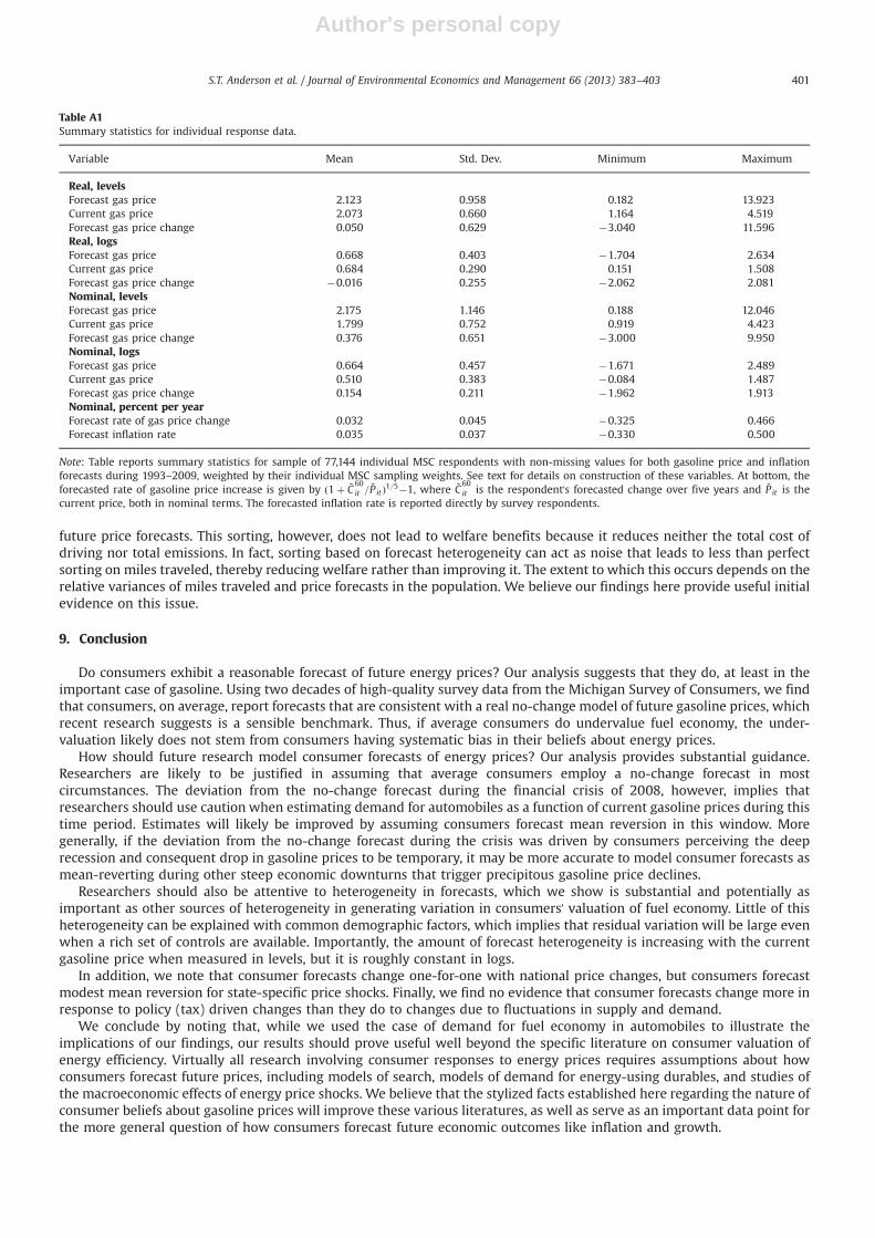
Author's personal copy
future price forecasts. This sorting, however, does not lead to welfare benefits because it reduces neither the total cost ofdriving nor total emissions. In fact, sorting based on forecast heterogeneity can act as noise that leads to less than perfectsorting on miles traveled, thereby reducing welfare rather than improving it. The extent to which this occurs depends on therelative variances of miles traveled and price forecasts in the population. We believe our findings here provide useful initialevidence on this issue.
9. Conclusion
Do consumers exhibit a reasonable forecast of future energy prices? Our analysis suggests that they do, at least in theimportant case of gasoline. Using two decades of high-quality survey data from the Michigan Survey of Consumers, we findthat consumers, on average, report forecasts that are consistent with a real no-change model of future gasoline prices, whichrecent research suggests is a sensible benchmark. Thus, if average consumers do undervalue fuel economy, the under-valuation likely does not stem from consumers having systematic bias in their beliefs about energy prices.
How should future research model consumer forecasts of energy prices? Our analysis provides substantial guidance.Researchers are likely to be justified in assuming that average consumers employ a no-change forecast in mostcircumstances. The deviation from the no-change forecast during the financial crisis of 2008, however, implies thatresearchers should use caution when estimating demand for automobiles as a function of current gasoline prices during thistime period. Estimates will likely be improved by assuming consumers forecast mean reversion in this window. Moregenerally, if the deviation from the no-change forecast during the crisis was driven by consumers perceiving the deeprecession and consequent drop in gasoline prices to be temporary, it may be more accurate to model consumer forecasts asmean-reverting during other steep economic downturns that trigger precipitous gasoline price declines.
Researchers should also be attentive to heterogeneity in forecasts, which we show is substantial and potentially asimportant as other sources of heterogeneity in generating variation in consumers' valuation of fuel economy. Little of thisheterogeneity can be explained with common demographic factors, which implies that residual variation will be large evenwhen a rich set of controls are available. Importantly, the amount of forecast heterogeneity is increasing with the currentgasoline price when measured in levels, but it is roughly constant in logs.
In addition, we note that consumer forecasts change one-for-one with national price changes, but consumers forecastmodest mean reversion for state-specific price shocks. Finally, we find no evidence that consumer forecasts change more inresponse to policy (tax) driven changes than they do to changes due to fluctuations in supply and demand.
We conclude by noting that, while we used the case of demand for fuel economy in automobiles to illustrate theimplications of our findings, our results should prove useful well beyond the specific literature on consumer valuation ofenergy efficiency. Virtually all research involving consumer responses to energy prices requires assumptions about howconsumers forecast future prices, including models of search, models of demand for energy-using durables, and studies ofthe macroeconomic effects of energy price shocks. We believe that the stylized facts established here regarding the nature ofconsumer beliefs about gasoline prices will improve these various literatures, as well as serve as an important data point forthe more general question of how consumers forecast future economic outcomes like inflation and growth.
Table A1Summary statistics for individual response data.
Variable Mean Std. Dev. Minimum Maximum
Real, levelsForecast gas price 2.123 0.958 0.182 13.923Current gas price 2.073 0.660 1.164 4.519Forecast gas price change 0.050 0.629 �3.040 11.596Real, logsForecast gas price 0.668 0.403 �1.704 2.634Current gas price 0.684 0.290 0.151 1.508Forecast gas price change �0.016 0.255 �2.062 2.081Nominal, levelsForecast gas price 2.175 1.146 0.188 12.046Current gas price 1.799 0.752 0.919 4.423Forecast gas price change 0.376 0.651 �3.000 9.950Nominal, logsForecast gas price 0.664 0.457 �1.671 2.489Current gas price 0.510 0.383 �0.084 1.487Forecast gas price change 0.154 0.211 �1.962 1.913Nominal, percent per yearForecast rate of gas price change 0.032 0.045 �0.325 0.466Forecast inflation rate 0.035 0.037 �0.330 0.500
Note: Table reports summary statistics for sample of 77,144 individual MSC respondents with non-missing values for both gasoline price and inflationforecasts during 1993–2009, weighted by their individual MSC sampling weights. See text for details on construction of these variables. At bottom, theforecasted rate of gasoline price increase is given by ð1þ ~C
60it =
~P it Þ1=5�1, where ~C60it is the respondent's forecasted change over five years and ~P it is the
current price, both in nominal terms. The forecasted inflation rate is reported directly by survey respondents.
S.T. Anderson et al. / Journal of Environmental Economics and Management 66 (2013) 383–403 401

Author's personal copy
Acknowledgments
We thank Richard Curtin for guidance in using the MSC data. For helpful comments, we also thank Hunt Allcott, SeverinBorenstein, Liran Einav, Lutz Kilian, Tim Vogelsang, Florian Zettelmeyer, and seminar participants at the ASSA meetings,Columbia University, Cornell University, Iowa State University, Michigan State University, Rice University, University ofCalifornia Berkeley, University of California Davis, University of California Energy Institute, University of California SantaBarbara, University of Chicago, University of Houston, University of Illinois, and University of Texas. We gratefullyacknowledge financial support from the California Energy Commission.
Appendix A
Table A1 presents summary statistics for the sample of 77,144 individual MSC respondents with non-missing values forboth gasoline price and inflation forecasts during 1993–2009.
Figs. A1 and A2 provide corollaries to Figs. 3 and 4 using logged values. Specifically, we log the individual values of thenominal and real gasoline price forecasts and then average across observations. These averages are used to generate the“Logs” results in Tables 2–4.
References
Allcott, Hunt, 2012. The Welfare Effects of Misperceived Product Costs: Data and Calibrations from the Automobile Market. NYU, manuscript.Allcott, Hunt, Wozny, Nathan, 2011. Gasoline Prices, Fuel Economy, and the Energy Paradox. MIT, manuscript.
−0.5
0
0.5
1
1.5
2
$/ga
llon,
nom
inal
(log
s)
Jan92 Jan94 Jan96 Jan98 Jan00 Jan02 Jan04 Jan06 Jan08 Jan10
Date
Mean forecastCurrent priceMean forecast change
Fig. A1. Nominal gasoline prices and forecasts in logs.
−0.5
0
0.5
1
1.5
2
$/ga
llon,
real
(log
s)
Jan92 Jan94 Jan96 Jan98 Jan00 Jan02 Jan04 Jan06 Jan08 Jan10
Date
Mean forecastCurrent priceMean forecast change
Fig. A2. Real gasoline prices and forecasts in logs.
S.T. Anderson et al. / Journal of Environmental Economics and Management 66 (2013) 383–403402

Author's personal copy
Allcott, Hunt, Mullainathan, Sendhil, Taubinsky, Dmitry, 2012. Externalities, Internalities, and the Targeting of Energy Policy, April 2012. NBER WorkingPaper 17977.
Alquist, Ron, Kilian, Lutz, 2010. What do we learn from the price of crude oil futures? Journal of Applied Econometrics 25 (June/July (4)), 539–573.Alquist, Ron, Kilian, Lutz, Vigfusson, Robert J., 2013. Forecasting the Price of oil. In: Graham Elliot, Allan Timmerman (Eds.), Handbook of Economic
Forecasting vol. 2. Elsevier, Amsterdam: North-Holland.Anderson, Soren T., Sallee, James M., 2011. Using loopholes to reveal the marginal cost of regulation: the case of fuel-economy standards. American
Economic Review 101 (June (4)), 1375–1409.Anderson, Soren. T., Kellogg, Ryan, Sallee, James. M., Curtin, Richard. T., 2011. Forecasting gasoline prices using consumer surveys. American Economic
Review Papers & Proceedings 101 (May (3)), 110–114.Bento, Antonio M., Li, Shanjun, Roth, Kevin, 2012. Is there an energy paradox in fuel economy? A note on the role of consumer heterogeneity and sorting
bias. Economics Letters 115 (April (1)), 44–48.Berry, Steven, Levinsohn, James, Pakes, Ariel, 1995. Automobile prices in market equilibrium. Econometrica 64 (July (4)), 841–890.Busse, Meghan R., Knittel, Christopher R., Zettelmeyer, Florian, 2013. Are consumers myopic? Evidence from new and used car purchases. American
Economic Review, 103 (1), 220–256.Curtin, Richard, 2010. Inflation expectations and empirical tests: theoretical models and empirical tests. In: Sinclair, Peter (Ed.), Inflation Expectations, vol.
56. , Routledge International Studies in Money and Banking, New York, pp. 34–61.Curtin, Richard T., 2004. Psychology and macroeconomics. In: Kahn, Robert L., Juster, F. Thomas, House, James S., Schuman, Howard, Singer, Eleanor (Eds.), A
Telescope on Society: Survey Research and Social Science at the University of Michigan & Beyond, University of Michigan Press, Ann Arbor.Davis, Lucas W., Kilian, Lutz, 2011. Estimating the effect of a gasoline tax on carbon emissions. Journal of Applied Econometrics 26, 1187–1214.Dubin, Jeffrey A., McFadden, Daniel L., 1984. An econometric analysis of residential electric appliance holdings and consumption. Econometrica 52 (March
(2)), 345–362.Elliott, Graham, Rothenberg, Thomas J., Stock, James H., 1996. Efficient tests for an autoregressive unit root. Econometrica 64 (July (4)), 813–836.Gillingham, Kenneth, 2011. How do consumers respond to gasoline price shocks? Heterogeneity in vehicle choice and driving behavior. Yale University,
manuscript.Goldberg, Pinelopi Koujianou, 1998. The effects of the corporate average fuel efficiency standards in the US. The Journal of Industrial Economics 46 (March
(1)), 1–33.Hamilton, James D., 2008. Oil and the macroeconomy. In: Durlauf, Steven N., Blume, Lawrence E. (Eds.), The New Palgrave Dictionary of Economics2nd ed. ,
Palgrave Macmillan.Hamilton, James D., 2009. Understanding crude oil prices. The Energy Journal 30 (2), 179–206.Hastings, Justine S., Shapiro, Jesse, 2011. Mental Accounting and Consumer Choice: Evidence from Commodity Price Shocks. University of Chicago,
manuscript.Kahn, James A., 1986. Gasoline prices and the used automobile market: a rational expectations asset price approach. The Quarterly Journal of Economics
101 (2), 323–339.Kilian, Lutz, Sims, Eric R., 2006. The Effects of Real Gasoline Prices on Automobile Demand: A Structural Analysis Using Micro Data. University of Michigan,
manuscript.Klier, Thomas, Linn, Joshua, 2010. New Vehicle Characteristics and the Cost of the Corporate Average Fuel Economy Standard. In: Resources for the Future
Discussion Paper, pp. 10–50.Knittel, Christopher R., Sandler, Ryan, Carbon prices and automobile greenhouse gas emissions: the extensive and intensive margins. In: Fullerton, Don,
Wolfram, Catherine (Eds.), The Design and Implementation of U.S. Climate Policy. National Bureau of Economic Research Conference Report, Universityof Chicago Press, September 2012. /http://press.uchicago.edu/ucp/books/book/chicago/D/bo13270829.htmS.
Langer, Ashley, Miller, Nathan H., 2011. Automakers' Short-Run Responses to Changing Gasoline Prices and the Implications for Energy Policy. University ofMichigan, manuscript.
Lewis, Matthew, Marvel, Howard P., 2011. When do consumers search? Journal of Industrial Economics 59 (September (3)), 457–483.Li, Shanjun, Timmins, Christopher, von Haefen, Roger H., 2009. How do gasoline prices affect fleet fuel economy? American Economic Journal: Economic
Policy 1 (August (2)), 113–137.Li, Shanjun, Linn, Joshua, Muehlegger, Erich, 2012. Gasoline Taxes and Consumer Behavior. Harvard University, manuscript.Linn, Joshua, Klier, Thomas, 2010. The price of gasoline and new vehicle fuel economy: evidence from monthly sales data. American Economic Journal:
Economic Policy 2 (August (3)), 134–153.Lu, S., 2006. Vehicle Survivability and Travel Mileage Schedules. Technical Report DOT HS 809 952, National Highway Traffic Safety Administration.Mankiw, N. Gregory, Reis, Ricardo, Wolfers, Justin, 2004. Disagreement about inflation expectations. In: Gertler, Mark, Rogoff, Kenneth (Eds.), NBER
Macroeconomics Annual 2003, vol. 18. , MIT Press, Cambridge, MA, pp. 209–247.Manski, Charles F., 2004. Measuring expectations. Econometrica 72 (September (5)), 1329–1376.Ng, Serena, Perron, Pierre, Lag, Length, 2001. Selection and the construction of unit root tests with good size and power. Econometrica 69 (November (6)),
1519–1554.Sallee, James M., West, Sarah E., Fan, Wei, 2009. Consumer valuation of fuel economy: a microdata approach. In: Proceedings of the National Tax Association
Annual Conference on Taxation.Small, Kenneth A., Van Dender, Kurt, 2007. Fuel efficiency and motor vehicle travel: the declining rebound effect. Energy Journal 28 (1), 25–51.van der Klaauw, Wilbert, Bruine de Bruin, Wändi, Topa, Giorgio, Potter, Simon, Bryan, Michael, 2008. Rethinking the Measurement of Household Inflation
Expectations: Preliminary Findings. Federal Reserve Bank of New York Staff Report No. 359.West, Sarah E., Williams III, Roberton C., 2007. Optimal taxation and cross-price effects on labor supply: estimates of the optimal gas tax. Journal of Public
Economics 91 (April), 593–617.Whitefoot, Katie, Fowlie, Meredith, Skerlos, Steven, 2011. Evaluating U.S. Reformed Corporate Average Fuel Economy Standards Using an Engineering
Attribute Selection Model. University of California, Berkeley, manuscript.
S.T. Anderson et al. / Journal of Environmental Economics and Management 66 (2013) 383–403 403