using a discrete -event simulation model to identify

Using a discrete-event simulation model to identify bottlenecks and

determine the efficiency in a maintenance workshop

Francois Marthinus Fredrick Venter

14118735

2017/09/28

Final Project report submitted in partial fulfilment of the requirements for the module

BPJ 420 Project

at the

Department Industrial and Systems Engineering

University of Pretoria

© University of Pretoria

DEPARTEMENT BEDRYFS- EN SISTEEMINGENIEURSWESE

DEPARTMENT OF INDUSTRIAL AND SYSTEMS ENGINEERING

FRONT PAGE FOR FINAL PROJECT DOCUMENT (BPJ 420) - 2017

Information with regards to the mini-dissertation

Title Using a discrete event simulation model to

identify bottlenecks and identify the efficiency

in a maintenance workshop.

Author Venter, F.M.F

Student number 14118735

Supervisor/s Van Laar, Z.

Date 2017/09/28

Keywords Simulation modelling, Maintenance practices,

Earthmoving vehicles, Bottlenecks, Efficiency

Abstract Developing a discrete event simulation model

based on key aspects in the maintenance

workshop in order to identify bottlenecks and

determine the efficiency of maintenance

practices.

Category Simulation modelling

Declaration

1. I understand what plagiarism is and I am aware of the University's policy in this regard.

2. I declare that this is my own original work

3. Where other people's work has been used (either from a printed source, internet or any other

source) this has been carefully acknowledged and referenced in accordance with

departmental requirements

4. I have not used another student's past work to hand in as my own

5. I have not allowed and will not allow, anyone to copy my work with the intention of handing it

in as his/her own work

Signature

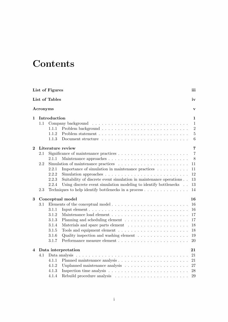
Contents

List of Figures iii

List of Tables iv

Acronyms v

1 Introduction 11.1 Company background . . . . . . . . . . . . . . . . . . . . . . . . . . . . . . 1

1.1.1 Problem background . . . . . . . . . . . . . . . . . . . . . . . . . . . 21.1.2 Problem statement . . . . . . . . . . . . . . . . . . . . . . . . . . . . 51.1.3 Document structure . . . . . . . . . . . . . . . . . . . . . . . . . . . 6

2 Literature review 72.1 Significance of maintenance practices . . . . . . . . . . . . . . . . . . . . . . 7

2.1.1 Maintenance approaches . . . . . . . . . . . . . . . . . . . . . . . . . 82.2 Simulation of maintenance practices . . . . . . . . . . . . . . . . . . . . . . 11

2.2.1 Importance of simulation in maintenance practices . . . . . . . . . . 112.2.2 Simulation approaches . . . . . . . . . . . . . . . . . . . . . . . . . . 122.2.3 Suitability of discrete event simulation in maintenance operations . . 132.2.4 Using discrete event simulation modeling to identify bottlenecks . . 13

2.3 Techniques to help identify bottlenecks in a process . . . . . . . . . . . . . . 14

3 Conceptual model 163.1 Elements of the conceptual model . . . . . . . . . . . . . . . . . . . . . . . . 16

3.1.1 Input element . . . . . . . . . . . . . . . . . . . . . . . . . . . . . . . 163.1.2 Maintenance load element . . . . . . . . . . . . . . . . . . . . . . . . 173.1.3 Planning and scheduling element . . . . . . . . . . . . . . . . . . . . 173.1.4 Materials and spare parts element . . . . . . . . . . . . . . . . . . . 183.1.5 Tools and equipment element . . . . . . . . . . . . . . . . . . . . . . 183.1.6 Quality inspection and washing element . . . . . . . . . . . . . . . . 193.1.7 Performance measure element . . . . . . . . . . . . . . . . . . . . . . 20

4 Data interpretation 214.1 Data analysis . . . . . . . . . . . . . . . . . . . . . . . . . . . . . . . . . . . 21

4.1.1 Planned maintenance analysis . . . . . . . . . . . . . . . . . . . . . . 214.1.2 Unplanned maintenance analysis . . . . . . . . . . . . . . . . . . . . 274.1.3 Inspection time analysis . . . . . . . . . . . . . . . . . . . . . . . . . 284.1.4 Rebuild procedure analysis . . . . . . . . . . . . . . . . . . . . . . . 29

i

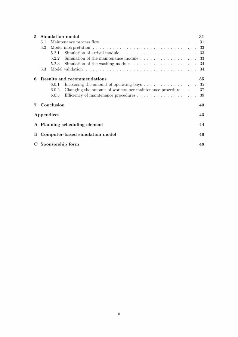
5 Simulation model 315.1 Maintenance process flow . . . . . . . . . . . . . . . . . . . . . . . . . . . . 315.2 Model interpretation . . . . . . . . . . . . . . . . . . . . . . . . . . . . . . . 33

5.2.1 Simulation of arrival module . . . . . . . . . . . . . . . . . . . . . . 335.2.2 Simulation of the maintenance module . . . . . . . . . . . . . . . . . 335.2.3 Simulation of the washing module . . . . . . . . . . . . . . . . . . . 34

5.3 Model validation . . . . . . . . . . . . . . . . . . . . . . . . . . . . . . . . . 34

6 Results and recommendations 356.0.1 Increasing the amount of operating bays . . . . . . . . . . . . . . . . 356.0.2 Changing the amount of workers per maintenance procedure . . . . 376.0.3 Efficiency of maintenance procedures . . . . . . . . . . . . . . . . . . 39

7 Conclusion 40

Appendices 43

A Planning scheduling element 44

B Computer-based simulation model 46

C Sponsorship form 48

ii

List of Figures

1.1 Duration of unplanned downtime . . . . . . . . . . . . . . . . . . . . . . . . 31.2 Duration of planned downtime . . . . . . . . . . . . . . . . . . . . . . . . . 4

2.1 Reactive maintenance model (Keith and Smith, 2008) . . . . . . . . . . . . 82.2 Proactive maintenance model (Keith and Smith,2008) . . . . . . . . . . . . 92.3 Comparing best practices benchmark . . . . . . . . . . . . . . . . . . . . . . 102.4 The five focusing steps . . . . . . . . . . . . . . . . . . . . . . . . . . . . . . 15

3.1 Maintenance load element . . . . . . . . . . . . . . . . . . . . . . . . . . . . 183.2 Materials and spare parts element . . . . . . . . . . . . . . . . . . . . . . . 193.3 Tools and equipment element . . . . . . . . . . . . . . . . . . . . . . . . . . 20

4.1 Distribution of the amount of EMV’s arriving per day for planned mainte-nance. . . . . . . . . . . . . . . . . . . . . . . . . . . . . . . . . . . . . . . . 22

4.2 Distribution of the amount of time it takes to complete a 250hr maintenancejob. . . . . . . . . . . . . . . . . . . . . . . . . . . . . . . . . . . . . . . . . . 23

4.3 Boxplot of the two different distributions in the 500hr maintenance procedure. 244.4 Distribution of the amount of time it takes to complete a 750hr maintenance

job. . . . . . . . . . . . . . . . . . . . . . . . . . . . . . . . . . . . . . . . . . 254.5 Boxplot of the 6000hr maintenance procedure . . . . . . . . . . . . . . . . . 264.6 Distribution of the amount of EMV’s arriving per day for unplanned main-

tenance. . . . . . . . . . . . . . . . . . . . . . . . . . . . . . . . . . . . . . . 284.7 Distribution of the amount time to perform a pre-inspection . . . . . . . . . 29

5.1 Current process flow of the workshop . . . . . . . . . . . . . . . . . . . . . . 32

6.1 Number of operating bays vs time reduction . . . . . . . . . . . . . . . . . . 36

A.1 Planning and scheduling element . . . . . . . . . . . . . . . . . . . . . . . . 45

B.1 Actual simulation model . . . . . . . . . . . . . . . . . . . . . . . . . . . . . 47

iii

List of Tables

1.1 Preventative maintenance per EMV type. . . . . . . . . . . . . . . . . . . . 21.2 Percentage of identified occurrences increasing the duration of planned and

unplanned downtime. . . . . . . . . . . . . . . . . . . . . . . . . . . . . . . . 4

2.1 Discrete-event simulation vs. agent-based simulation. . . . . . . . . . . . . . 13

4.1 Probabilities of occurrence for the different maintenance procedures. . . . . 274.2 Different rebuild events. . . . . . . . . . . . . . . . . . . . . . . . . . . . . . 30

5.1 Validation criteria of the simulation model. . . . . . . . . . . . . . . . . . . 34

6.1 Percentage of time reductions and duration of downtime for different amountsof operating bays. . . . . . . . . . . . . . . . . . . . . . . . . . . . . . . . . . 36

6.2 Utilisation of workers at different maintenance procedures. . . . . . . . . . . 376.3 Change in worker utilisation for the 750-hr and 6000-hr maintenance pro-

cedures for different amount of workers. . . . . . . . . . . . . . . . . . . . . 386.4 Efficiency measurements of the different maintenance procedures . . . . . . 39

iv

Acronyms

AMP Anglo American Platinum

EMV Earth Moving Vehicle

OEE Overall Equipment Effectiveness

BMP Best Maintenance Practices

PM Preventative Maintenance

CBM Condition Based Maintenance

TOC Theory of Constraints

FFS Five Focusing Steps

ABS Agent Based Simulation

DES Discrete Event Simulation

IMIS Inventory Management Information System

RI Resonant Industrial

v

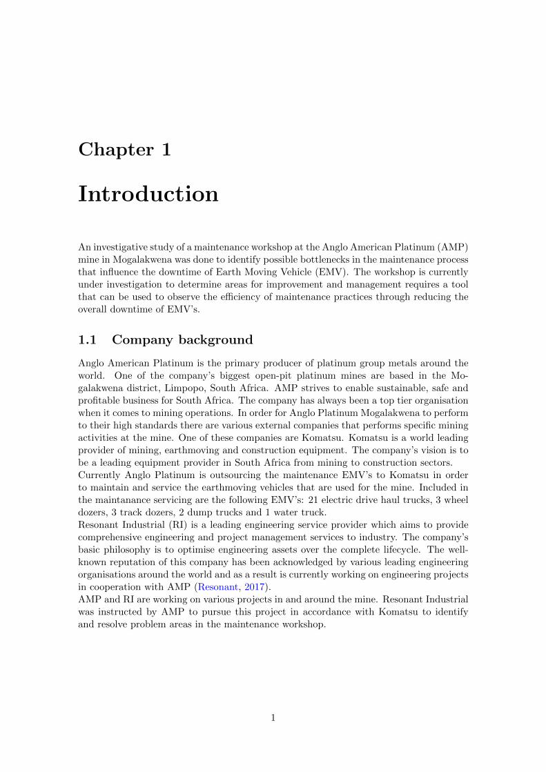
Chapter 1

Introduction

An investigative study of a maintenance workshop at the Anglo American Platinum (AMP)mine in Mogalakwena was done to identify possible bottlenecks in the maintenance processthat influence the downtime of Earth Moving Vehicle (EMV). The workshop is currentlyunder investigation to determine areas for improvement and management requires a toolthat can be used to observe the efficiency of maintenance practices through reducing theoverall downtime of EMV’s.

1.1 Company background

Anglo American Platinum is the primary producer of platinum group metals around theworld. One of the company’s biggest open-pit platinum mines are based in the Mo-galakwena district, Limpopo, South Africa. AMP strives to enable sustainable, safe andprofitable business for South Africa. The company has always been a top tier organisationwhen it comes to mining operations. In order for Anglo Platinum Mogalakwena to performto their high standards there are various external companies that performs specific miningactivities at the mine. One of these companies are Komatsu. Komatsu is a world leadingprovider of mining, earthmoving and construction equipment. The company’s vision is tobe a leading equipment provider in South Africa from mining to construction sectors.Currently Anglo Platinum is outsourcing the maintenance EMV’s to Komatsu in orderto maintain and service the earthmoving vehicles that are used for the mine. Included inthe maintanance servicing are the following EMV’s: 21 electric drive haul trucks, 3 wheeldozers, 3 track dozers, 2 dump trucks and 1 water truck.Resonant Industrial (RI) is a leading engineering service provider which aims to providecomprehensive engineering and project management services to industry. The company’sbasic philosophy is to optimise engineering assets over the complete lifecycle. The well-known reputation of this company has been acknowledged by various leading engineeringorganisations around the world and as a result is currently working on engineering projectsin cooperation with AMP (Resonant, 2017).AMP and RI are working on various projects in and around the mine. Resonant Industrialwas instructed by AMP to pursue this project in accordance with Komatsu to identifyand resolve problem areas in the maintenance workshop.

1

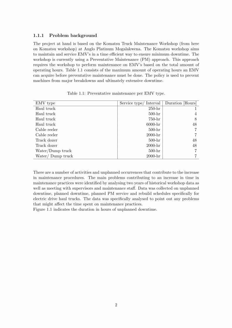
1.1.1 Problem background

The project at hand is based on the Komatsu Truck Maintenance Workshop (from hereon Komatsu workshop) at Anglo Platinum Mogalakwena. The Komatsu workshop aimsto maintain and service EMV’s in a time efficient way to ensure minimum downtime. Theworkshop is currently using a Preventative Maintenance (PM) approach. This approachrequires the workshop to perform maintenance on EMV’s based on the total amount ofoperating hours. Table 1.1 consists of the maximum amount of operating hours an EMVcan acquire before preventative maintenance must be done. The policy is used to preventmachines from major breakdowns and ultimately extensive downtime.

Table 1.1: Preventative maintenance per EMV type.

EMV type Service type/ Interval Duration [Hours]

Haul truck 250-hr 1Haul truck 500-hr 4Haul truck 750-hr 8Haul truck 6000-hr 48Cable reeler 500-hr 7Cable reeler 2000-hr 7Track dozer 500-hr 48Track dozer 2000-hr 48Water/Dump truck 500-hr 7Water/ Dump truck 2000-hr 7

There are a number of activities and unplanned occurrences that contribute to the increasein maintenance procedures. The main problems contributing to an increase in time inmaintenance practices were identified by analysing two years of historical workshop data aswell as meeting with supervisors and maintenance staff. Data was collected on unplanneddowntime, planned downtime, planned PM service and rebuild schedules specifically forelectric drive haul trucks. The data was specifically analysed to point out any problemsthat might affect the time spent on maintenance practices.Figure 1.1 indicates the duration in hours of unplanned downtime.

2

0 1000 2000 3000 4000

010

020

030

040

050

060

070

0Duration of unplanned downtime

Amount of EMV's

Dur

atio

n of

mai

nten

ance

[hou

rs]

Figure 1.1: Duration of unplanned downtime

Statistical analyses of Figure 1.1 showed that over the period of two years a standard likeaverage of 3 hours per EMV for unplanned downtime was obtained.This was verified bythe supervisor and maintenance staff which agreed that 3 hours is the normal rate at whichan unplanned occurrence usually takes before it is resolved. Thus by using this benchmarkall points on Figure 1.1 that is above 3 hours was illustrated as a red circle. The pointsrepresenting the outliers were investigated to determine the cause which produced theincrease in unplanned downtime.The number of points above the recommended 3 hours for unplanned downtime was 18.7%of the total points in the two year period. This indicated that 18.7% of the time it takesmore than three hours to get maintenance done on an EMV with the maximum time being626 hours or 26 days. This extreme occurrence was caused by the waiting time to receivethe required part in which in this case was a new engine.Planned downtime was analysed according to the PM policy on the total allowed oper-ating hours per EMV before maintenance is required (see Table 1.1). This means thatthe downtime was planned according to the type of service needed. Figure 1.2 indicatesthe duration of planned downtime per EMV. The outliers were investigated to determinethe cause of such a significant increase in downtime. Table 1.1 indicates that the max-imum amount of time an EMV should spend in the maintenance workshop undergoingPM maintenance is 48 hours. However the outliers indicated that there are some pointsexceeding the 48 hour limit. The data indicated that of the total planned downtime, 2.23%exceeds the 48 hour limit with the maximum downtime being 713 hours or 30 days. Thissignificant duration of downtime was caused by unavailability of parts. Also due to anincrease in maintenance activities the working bays were occupied and the EMV had to

3

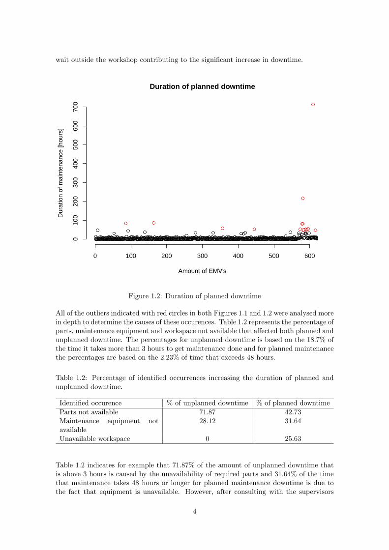
wait outside the workshop contributing to the significant increase in downtime.

0 100 200 300 400 500 600

010

020

030

040

050

060

070

0

Duration of planned downtime

Amount of EMV's

Dur

atio

n of

mai

nten

ance

[hou

rs]

Figure 1.2: Duration of planned downtime

All of the outliers indicated with red circles in both Figures 1.1 and 1.2 were analysed morein depth to determine the causes of these occurences. Table 1.2 represents the percentage ofparts, maintenance equipment and workspace not available that affected both planned andunplanned downtime. The percentages for unplanned downtime is based on the 18.7% ofthe time it takes more than 3 hours to get maintenance done and for planned maintenancethe percentages are based on the 2.23% of time that exceeds 48 hours.

Table 1.2: Percentage of identified occurrences increasing the duration of planned andunplanned downtime.

Identified occurence % of unplanned downtime % of planned downtime

Parts not available 71.87 42.73Maintenance equipment notavailable

28.12 31.64

Unavailable workspace 0 25.63

Table 1.2 indicates for example that 71.87% of the amount of unplanned downtime thatis above 3 hours is caused by the unavailability of required parts and 31.64% of the timethat maintenance takes 48 hours or longer for planned maintenance downtime is due tothe fact that equipment is unavailable. However, after consulting with the supervisors

4

and maintenance staff from the Komatsu workshop it was pointed out that an increase indowntime is not only caused by the reasons listed in Table 1.2 but due to work overloadand waiting time for EMV operators which can not be statistically analysed.

1.1.2 Problem statement

Currently the workshop is under a lot of pressure to try and increase the overall efficiency ofthe maintenance process by minimising the downtime per EMV. After consulting with theKomatsu supervisors and maintenance staff and analysing the data above, a list of prob-lems contributing to the increase in downtime and inefficient practices were constructed.The major problems currently active in the workshop are:

1. lack of workspace;

2. spare parts are not constantly available;

3. critical equipment is not constantly available;

4. maintenance procedures can be inefficient; and

5. maintenance staff is unavailable.

All of these problems contribute to the downtime of EMV’s which in effect reduces theefficiency of the overall workshop. Thus an opportunity exist to determine the efficiencyof the workshop practices and to identify potential bottlenecks that causes the increase indowntime of the EMV’s. In order to analyse these problems a simulation model will bedeveloped to incorporate the maintenance process. The simulation model will provide per-formance measures that can be analysed to determine what specific maintenance practicescontribute to downtime and in effect inefficiency of the overall workshop.

5

1.1.3 Document structure

In Chapter 2 a literature review describes and compares various different maintenance andsimulation approaches and techniques that will be used to build a conceptual simulationmodel. The literature in Chapter 2 also contains previous work done by various differentauthors on simulation techniques used to model maintenance approaches as well as usingthese simulation models to identify bottlenecks in a process.Chapter 3 of this report contains the conceptual simulation model that will be used toconstruct the actual model. This chapter explains the different elements that will beused in the simulation model as well as the different inputs and parameters that willbe analysed throughout the simulation process. Chapter 4 refers to the data analysesand data interpretation. The data is explained and analysed on different aspects of themaintenance process. Chapter 5 refers to the actual computer based simulation modelwhich interprets the current maintenance workshop. Chapter 6 refers to the results andrecommendations obtained explaining the model outputs. Chapter 7 is the conclusion ofthe report.

6

Chapter 2

Literature review

Maintenance practices have always been an important area for improvement in miningindustries, especially for cost saving strategies and availability of operational equipment.By examining maintenance practices and understanding the internal and external forcesinfluencing the maintenance process a platform can be created to determine the efficiencyand identify areas of improvement in maintenance workshops. Maintenance can thus beexamined as an efficient way to improve the overall productivity and output of a productionprocess.According to Alabdulkarim et al. (2015), maintenance operations can be complex to moni-tor. Therefore Lightfoot et al. (2011) suggests using applicable monitoring technology thatcan incorporate the complexities of a maintenance process. Decision making tools suchas simulation models provide a playground where different scenarios in the maintenanceworkshop can be created and ultimately be examined and analysed effectively withoutaffecting the real system.

2.1 Significance of maintenance practices

Maintenance can be described as the preserving and continuing of an entity in good operat-ing condition (Smith, 2004). Maintenance is becoming a crucial factor worth investigatingfor companies which aims to increase profitability, labour productivity and product qual-ity (Noemi and Leigh, 1993). As the complexity of operating equipment increases, therequired level of maintenance expertise increases.Noemi and Leigh (1993) states that along with the increase in maintenance complexity, themaintenance and production cost increases and companies are forced to develop mainte-nance practices which can operate at the most cost effective way. According to Abdulnouret al. (1995) maintenance management is responsible for reducing equipment downtimeand cost associated with unplanned disruptions. Unplanned downtime of a process indi-cates that activities responsible for the operation and flow of the process is currently atstandstill due to unforseen ciscumstances. If a company is not prepared for a downtimeto take place then ultimately profit is lost due to the increase in production and mainte-nance costs. However, Alabdulkarim et al. (2015) states that if maintenance managementfocuses on reducing unplanned downtime, maintenance cost and consequently productioncost will be reduced.

7

2.1.1 Maintenance approaches

Maintenance can add substantial value to a company’s reliability and can preserve it’sassets if it is developed and managed properly. Over the years different maintenanceapproaches emerged to help companies manage maintenance operations effectively. Ac-cording to Keith and Smith (2008) there are two main approaches. Reactive and proactivemaintenance. The reactive approach responds immediately to an identified need or requestin a production process. As can be seen in Figure 2.1 there are four main activities thattakes place primarily with the focus to perform maintenance operations. These primaryactivities include notification, planning, scheduling and fix. The other five activities aresecondary activities which only reacts to an order from a primary activity. For example,if maintenance is required a notification is sent out to a mechanic which then assessesthe problem and determines the tools and parts required to perform the maintenance.Planning and scheduling of the maintenance procedure takes place after the assessment.The mechanic then executes the maintenance activity using the necessary parts and tools.The goal of this approach is to minimise response time and reduce equipment downtime.The reactive approach also incorporates preventative maintenance and is used by mostcompanies today (Keith and Smith, 2008).

Figure 2.1: Reactive maintenance model(Keith and Smith, 2008)

The proactive approach contains more predictive measures and primarily reacts to equip-ment assessment. Figure 2.2 indicates the proactive maintenance model. The model beginsthe process with predictive procedures which includes daily and weekly inspections. Theinspections include performance evaluation and as a result it can be monitored whetherthere is a need to perform maintenance to ensure prevention of future breakdowns. Alsothe model incorporates data on work performance that is gathered over the years to predictwhether maintenance is necessary. After the evaluation, planning takes place. The plan-ning phase is used to determine the type of work order/maintenance procedure that will beexecuted. When a work order is established a problem solving team is dispatched to per-form the necessary maintenance required. After the maintenance is completed the processstarts again with predictive procedures such as inspections with the help of historically

8

work performance. The goal of this approach is to maintain continuous improvement in aproduction process by focusing on equipment performance, specifications and maintenanceof productive capacity.

Figure 2.2: Proactive maintenance model (Keith and Smith, 2008)

These two approaches identified by (Keith and Smith, 2008) lay the foundation of morespecific and developed maintenance approaches which can be implemented by companiesto fit their needs and requirements.One of these approaches are Best Maintenance Practices (BMP), developed by Smith(2004). According to Smith (2004) “ it represents benchmarking standards that are real,specific and achievable for maintenance management”. The following points are the bench-marking standards formulated by Smith (2004):

• work orders must always cover 100% of the maintenance personnel’s time;

• preventative maintenance inspections must generate 90% of work orders;

• at least 30% of total labour hours are from preventative maintenance;

• planned or scheduled work must be executed 90% the time;

• total reliability is reached 100% of the time;

• overall equipment effectiveness (OEE) is greater than 85%; and

• only 2% of total maintenance time must be overtime.

Smith (2004) identified the opportunity to effectively establish standards to which mainte-nance practices can be compared. The aim of BMP is to achieve more efficient maintenanceareas, reduce maintenance costs and improve reliability and increased confidence of main-tenance staff. Smith (2004) goes on to say that it is important to identify the reasons for amaintenance workshop not achieving BMP. The two most common reasons that a facilitydoes not follow BMP are that current maintenance is sensitive to failure and in turn failsto safeguard maintenance practices as well as workforce in the maintenance department

9

lacks the ability and discipline to follow BMP as well as management failing to define rulesof conduct for BMP.Smith (2004) states that management should actively pursue a proactive thinking whenit comes to maintenance ineffectiveness. By combining a proactive approach with BMP,maintenance effectiveness will improve rapidly.In the work of (Smith, 2004) it is stated that a leading global management consulting firmimplemented a BMP proactive thinking approach to the maintenance operations of thecompany and within a period of three years the following results were obtained:

• increase in productivity of 28.2%;

• maintenance cost decrease of 19.4%;

• equipment availability and reliability increase of 20.1%; and

• reduction in inventory carrying cost of 17.8%.

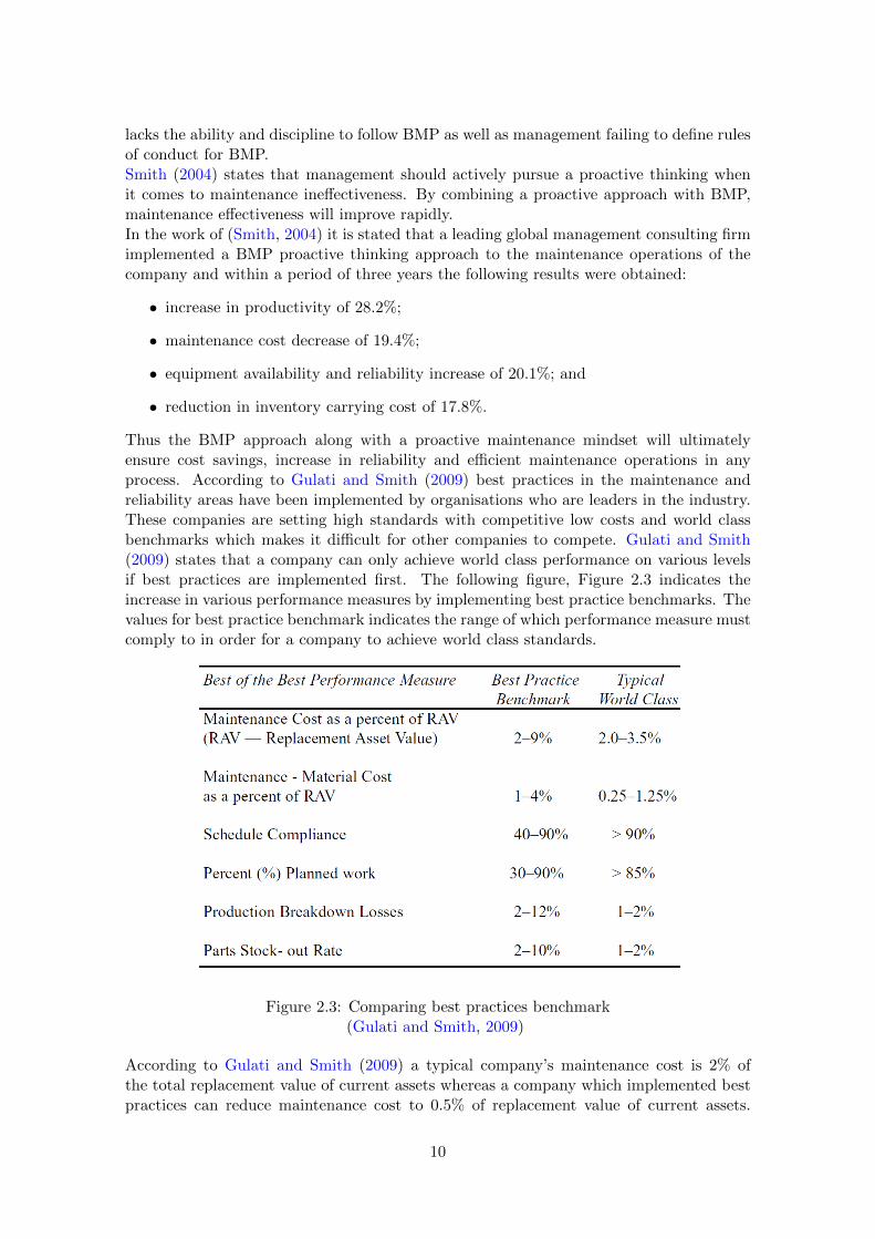
Thus the BMP approach along with a proactive maintenance mindset will ultimatelyensure cost savings, increase in reliability and efficient maintenance operations in anyprocess. According to Gulati and Smith (2009) best practices in the maintenance andreliability areas have been implemented by organisations who are leaders in the industry.These companies are setting high standards with competitive low costs and world classbenchmarks which makes it difficult for other companies to compete. Gulati and Smith(2009) states that a company can only achieve world class performance on various levelsif best practices are implemented first. The following figure, Figure 2.3 indicates theincrease in various performance measures by implementing best practice benchmarks. Thevalues for best practice benchmark indicates the range of which performance measure mustcomply to in order for a company to achieve world class standards.

Figure 2.3: Comparing best practices benchmark(Gulati and Smith, 2009)

According to Gulati and Smith (2009) a typical company’s maintenance cost is 2% ofthe total replacement value of current assets whereas a company which implemented bestpractices can reduce maintenance cost to 0.5% of replacement value of current assets.

10

Thus increasing the replacement value for assets in a company and increasing overall netincome. Also, Gulati and Smith (2009) states that the percentage of planned work canincrease from 30% for a typical company to 90% for a best practice company. This increaseis due to the fact that the company is proactively planning three times more work andwill ultimately have higher up time and high utilization rates.Preventative maintenance (PM) approach is described by Andriulo et al. (2015) as sched-uled activities according to predetermined time intervals. The aim of PM is to conductmaintenance activities on a scheduled basis in order to prevent as much as possible fail-ures. However, Alabdulkarim et al. (2015) argues that PM has a shortfall. This ap-proach performs maintenance on a periodic basis regardless whether the asset is in needof maintenance or not. Thus by performing unnecessary maintenance activities the costof maintenance becomes very high.Grall et al. (2002) reckons that Condition-Based Maintenance (CBM) is a more efficientapproach than preventative maintenance. CBM takes into account the health status ofthe asset. This is done through inspection and sensing technologies. CBM consists of twomonitoring levels namely diagnostics and prognostics. The diagnostic level is when thecomponent/machine diagnoses itself when a failure occur and gives feedback to a main-tenance centre. Prognostics is when the component/machine consists of monitoring andsensing technology and predicts a failure based on the health of the component/machine(Alabdulkarim et al., 2015).Ultimately there are numerous maintenance approaches that have been developed andimplemented across various different systems and processes. The greatest effect a mainte-nance approach will have on any kind of system or process is when an approach is thor-oughly investigated to address the specific needs and requirements of a company. Thusby using previous literature and research on maintenance approaches one can identify thebest option which will satisfy all needs in a company.

2.2 Simulation of maintenance practices

Simulation as described by Tiwari and Alrabghi (2016) is a decision making tool that canbe used to build different types of models to incorporate complex systems. A simulationmodel in effect can be developed to mimic a process to such an extent that by changingparameters and inputs in the model one can see what effect it will have on a real worldprocess without affecting the system.Tiwari and Alrabghi (2016) reckons that although maintenance systems are complex, withthe use of simulation modeling these systems can be understood and improved effectively.

2.2.1 Importance of simulation in maintenance practices

According to Duffuaa et al. (2001) it is important to understand the complexity of mainte-nance systems. Maintenance systems interact with other complex subsystems like procure-ment processes for required parts. Also it is difficult to measure the output of maintenancein a quantifiable way and many uncertain elements exists in maintenance systems such asjob arrival rates and time needed to perform maintenance (Duffuaa et al., 2001). All ofthese points contribute to the complexity of maintenance systems.According to Alabdulkarim et al. (2015) the use of simulation has been widely used inhealthcare, defence and public services. The different techniques in simulation can beused to analyse the performance of any operating system without affecting the real sys-tem. Alabdulkarim et al. (2015) states that because simulation is appropriate to monitor

11

detailed operation systems it is relevant to maintenance systems as well.Pannirselvam et al. (1999) argues that simulation is voted as the second most widelyused monitoring technique in operations management and has the ability to represent thecomplexity of maintenance systems.In the work done by Savsar (1990) the relationship between simulation and maintenancesystems were studied to investigate the effect of different maintenance policies on produc-tion. It was concluded that simulation can also be used to find the optimal number ofmaintenance staff as well as optimal inventory in production systems.In the work done by Joo et al. (1997) a simulation model was specifically developed toanalyse a preventative maintenance approach with the main goal to improve efficiency.The average equipment utilization and average waiting time were used as measures ofperformance.Mosley et al. (1998) developed a maintenance scheduling simulation model with the mainobjective to minimise downtime by scheduling only the necessary maintenance equipmentand staff for the required job.

2.2.2 Simulation approaches

Nowadays there are various different simulation techniques that can be used as tools torepresent complex processes and systems. It is critical to know the merits and shortfallsof a simulation technique. By knowing the capability of these techniques the modeler canavoid any limits or complexity in the quest to build an effective, accurate model.The research conducted in this section of the literature review only includes two approachesto simulation modeling. Discrete Event Simulation (DES) and Agent Based Simulation(ABS).

Discrete-event simulation vs. Agent-based simulation

According to Baldwin et al. (2015) most model types have different perspectives on sys-tems. One perspective is looking down on a system and the other is looking up from thesystem. DES follows a looking down perspective by modeling different events and ABSfollows a looking up perspective that takes into account the functionality of the system.Baldwin et al. (2015) states that ABS creates a model based on a collection of agents(autonomous decision making entities). The agents individually assess the situation fromwhich it can make a decision based on a set of rules (Bonabeau, 2002). Baldwin et al. (2015)states that agents can be people, social factors, organizations or any individual system,the only requirement is that these agents must work independently of their environment.ABS can also be used for hypotheses testing to reveal whether an expected outcome willoccur.Discrete event simulation according to Baldwin et al. (2015) focuses on externally observ-able events that occur in different stages in a system. In other words, DES represent acollection of events that influence the system. Tiwari and Alrabghi (2016) states that theevents in a DES are modeled as a queue and executed one by one as the simulation movesthrough the model.Table 2.1 consists comparisons of discrete event simulation and agent based simulation.As (Baldwin et al., 2015) states that one cannot predict whether DES or ABS will workbetter for modeling based on evaluating the merits and shortfalls of these two techniques.However, a decision must be made on whether the technique can address the specificpurposes and needs of an organisation.

12

Table 2.1: Discrete-event simulation vs. agent-based simulation.

Discrete-event simulation Agent-based simulation

Model creation is simple and easy under-standable.

Model logic is complicated by the flexibil-ity of agents.

Observes external events. Observes decision making agents (entities).Respond to discrete events. Respond to functionality of agents.State of system changes in response toevents.

Agents are flexible and independent.

Events can impact the entire simulation. Agents function as distinct parts.Easy to validate. Difficult to test.

2.2.3 Suitability of discrete event simulation in maintenance operations

According to Alabdulkarim et al. (2015) discrete event simulation has the potential toassess various maintenance approaches by taking into account all the maintenance char-acteristics like labour availability, spare part availability, asset location and travel timebetween assets. In the automotive industry a study conducted by Ali et al. (2008) useddiscrete event simulation to identify bottlenecks and optimise maintenance strategies. Aliet al. (2008) discovered that the overall availability in the production system has decreasedas a result of excessive downtime due to machine/equipment failures.Greasley (2000) developed a DES model for a maintenance project involving trains. Thecompany benefited from the operational impacts by developing a variety of plans and waysto meet demand.The Finnish Air Force also developed a DES model to monitor the effects of policies,maintenance resources and availability of aircrafts in different environments (Mattila et al.,2008).Although DES is one of the few simulating techniques that can combine all the complexsubsystems of a maintenance system (Tiwari and Alrabghi, 2016), studies in this area islimited (Alabdulkarim et al., 2015).

2.2.4 Using discrete event simulation modeling to identify bottlenecks

According to Lavoie et al. (2009) a discrete event simulation (DES) model is the preferredapproach to evaluate the impact of dynamic aspects of processing plants. Lavoie et al.(2009) also states that it is a tool that can be used to identify bottlenecks in a plant,evaluate the response on implementing new technology in the plant, evaluate the impacton the plant if the workspace increases and optimize maintenance and operating practiceswithout disrupting the operation.The challenges faced in the iron ore plants were that production systems are very com-plex. This complexity made it a very difficult task to estimate the benefits of projectsin existing operations. Adding to the effect was equipment reliability and maintenanceschedules of which a shift in bottlenecks occurred frequently. To deal with this problem adynamic simulation model was created based on specific system characteristics to exploitbottlenecks by creating different production scenarios.Lavoie et al. (2009) states that DES is the most effective and comprehensive simulationapproach to date to evaluate the production performance of complex systems. The modelcan interpret basic operations that mimic the behavior of a system. A key attribute of

13

the DES is that it can reproduce elements of the system using representative statisticaldistributions. Other simulation approaches were also investigated by (Lavoie et al., 2009)like analytical models and Monte Carlo simulations but ruled out. Analytical modelsrequire real-world problems to be simplified to a point where they are not useful anymoreand Monte Carlo simulations becomes less user-friendly over time when scheduled eventssuch as maintenance must be incorporated.The main and most important part of the project was the validation and sensitivity anal-ysis of the simulation model. Lavoie et al. (2009) describes the aspects of validating aDES model as well as performing a sensitivity analyses. According to Lavoie et al. (2009)verification and validation is done in two steps:

1. Verify model calculations against an existing steady state model, for example likethroughputs, yields, mass balances etc. The first step is done to indicate whetherthe results of the model would give similar outputs when events like scheduled andunscheduled downtime were ignored (when scheduled and unscheduled downtime isignored the plant is in a steady state).

2. Validate the dynamics of the model - Lavoie et al. (2009) used historical plant per-formance data to compare the model results.According to Lavoie et al. (2009) the sensitivity analyses helped to validate themodel by examining the effect it had to changes made in different input variables.By changing the inputs of the model an increase of ten per cent in filter and ballingcapacity were observed. This increase indicated a bottleneck in the process.

These two steps indicate the functionality of using discrete event simulation in order toidentify potential bottlenecks in a process.

2.3 Techniques to help identify bottlenecks in a process

In any process or system it is often found that a constraint occur. A constraint in a processis a restriction that can limit the functionality and availability of resources needed in aprocess. According to Petersen et al. (2014) the negative impact a constraint can have inany process includes work overload, decrease in overall efficiency, delays and requirementsbecome obsolete and creates stress in the organization.The most effective and fastest way to improve efficiency and profitability in a processis by identifying and eliminating constraints. Theory of Constraints (TOC) is a methoddesigned by Dr. Eliyahu Goldratt to help identify constraints. In manufacturing processesa constraint is usually referred to as a bottleneck. The TOC provides a set of tools toenable companies to identify potential bottlenecks. The tools include:

1. The Five Focusing Steps;

This tool provides a method for identifying and eliminating bottlenecks in a process.

2. The Thinking Process

This tool enables companies to analyse and resolve any problems that occur in aprocess.

3. Throughput Accounting

This tool provides a method that measures performance as well as assist in manage-ment decisions.

14

Companies that implement TOC not only improve profitability and efficiency but alsoobtain various other benefits like system and processes improve at a fast rate, productioncapacity increases which means that more products can be manufactured, reduction in leadtimes, increase in product flow and reduction in inventory ensures less work-in-process.The TOC contains a specific method for identifying bottlenecks. The Five Focusing Steps(FFS) described above is used to identify bottlenecks. Figure 2.4 illustrates a diagram ofthese five steps.

Figure 2.4: The five focusing steps

The implementation of these five steps will ultimately enable the exploitation of bottle-necks in a process.

15

Chapter 3

Conceptual model

The development of a conceptual model is subjected to the various specifications and ele-ments in a maintenance process. The conceptual model will lead to a better understandingof the maintanance processes by exploiting their complexities. The specifications of theconceptual model lays the foundation for developing a simulation model (Duffuaa et al.,2001).The specifications and elements of the conceptual model was based on the realistic charac-teristics of the Komatsu maintenance workshop. The conceptual model consists of sevenelements each interpreting the specifications in the Komatsu workshop.

3.1 Elements of the conceptual model

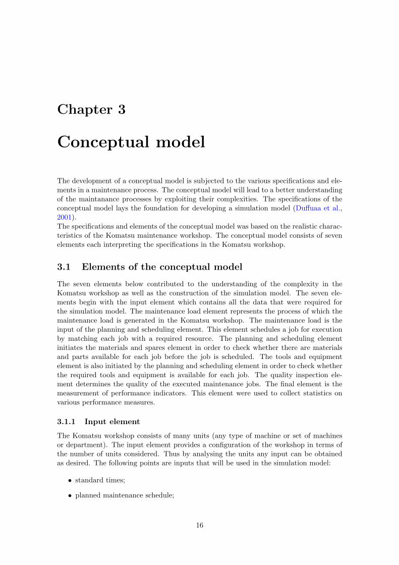
The seven elements below contributed to the understanding of the complexity in theKomatsu workshop as well as the construction of the simulation model. The seven ele-ments begin with the input element which contains all the data that were required forthe simulation model. The maintenance load element represents the process of which themaintenance load is generated in the Komatsu workshop. The maintenance load is theinput of the planning and scheduling element. This element schedules a job for executionby matching each job with a required resource. The planning and scheduling elementinitiates the materials and spares element in order to check whether there are materialsand parts available for each job before the job is scheduled. The tools and equipmentelement is also initiated by the planning and scheduling element in order to check whetherthe required tools and equipment is available for each job. The quality inspection ele-ment determines the quality of the executed maintenance jobs. The final element is themeasurement of performance indicators. This element were used to collect statistics onvarious performance measures.

3.1.1 Input element

The Komatsu workshop consists of many units (any type of machine or set of machinesor department). The input element provides a configuration of the workshop in terms ofthe number of units considered. Thus by analysing the units any input can be obtainedas desired. The following points are inputs that will be used in the simulation model:

• standard times;

• planned maintenance schedule;

16

• unplanned maintenance schedule (Breakdowns);

• plant configuration (number of units);

• staff job cards;

• spare parts requirements;

• critical equipment requirements;

• downtime of overall workshop practices; and

• historical maintenance data from the SAP system.

3.1.2 Maintenance load element

There are two main maintenance load elements in the workshop.

1. Planned maintenance load

In the workshop this load is known in advance and provides job schedules, availabilityof spare parts and tools and equipment requirements. This is all planned accordingto when an EMV is scheduled for maintenance based on the amount of operatinghours it completed.

2. Unplanned maintenance load

The unplanned maintenance load is an instant occurrence that can happen at anygiven time. For the workshop this load is mostly dominated by breakdowns. Al-though it can not be predicted, historical data can show the pattern of occurrenceand what elements are effected by it.

The flow chart in Figure 3.1 below indicates how the maintenance load is formed byplanned and unplanned maintenance.

3.1.3 Planning and scheduling element

The planning and scheduling element is the core of the simulation model. The maintenanceload consisting of planned and unplanned maintenance will be the input into this element.When the EMV arrives at the workshop the following steps are carried out in the simulationmodel:The planning and scheduling element can be seen in Figure A.1 Appendix A.

1. Check priority level

The model determines the maintenance priority for each EMV that arrives at theworkshop.

2. Check parts availability and staff availability.

The model will determine whether there are maintenance staff available to executea job with the required parts needed.

3. Check tools and equipment availability.

This element will determine whether key equipment, tools are available for mainte-nance procedures.

17

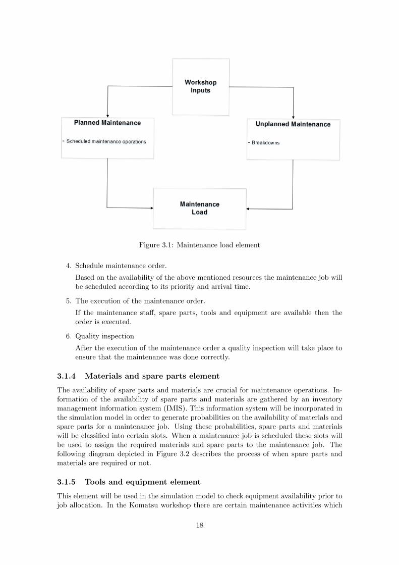
Figure 3.1: Maintenance load element

4. Schedule maintenance order.

Based on the availability of the above mentioned resources the maintenance job willbe scheduled according to its priority and arrival time.

5. The execution of the maintenance order.

If the maintenance staff, spare parts, tools and equipment are available then theorder is executed.

6. Quality inspection

After the execution of the maintenance order a quality inspection will take place toensure that the maintenance was done correctly.

3.1.4 Materials and spare parts element

The availability of spare parts and materials are crucial for maintenance operations. In-formation of the availability of spare parts and materials are gathered by an inventorymanagement information system (IMIS). This information system will be incorporated inthe simulation model in order to generate probabilities on the availability of materials andspare parts for a maintenance job. Using these probabilities, spare parts and materialswill be classified into certain slots. When a maintenance job is scheduled these slots willbe used to assign the required materials and spare parts to the maintenance job. Thefollowing diagram depicted in Figure 3.2 describes the process of when spare parts andmaterials are required or not.

3.1.5 Tools and equipment element

This element will be used in the simulation model to check equipment availability prior tojob allocation. In the Komatsu workshop there are certain maintenance activities which

18

Figure 3.2: Materials and spare parts element

requires specific tools and equipment like an overhead crane or forklift. However, becauseof the limited space in the working area the availability of these critical tools are limited.Only the critical tools and equipment is considered in this element. Probabilities willbe assigned to these tools to determine their availability for a maintenance job and canthus be modeled in the simulation. The following diagram in Figure 3.3 describes thelogic the simulation model will follow when determining and assigning the critical tools tomaintenance jobs.

3.1.6 Quality inspection and washing element

After a maintenance job is completed, the quality of the work done is checked to ensurethat required quality standards have been met. After the inspection the EMV will becleaned/washed. Although this activity seems unnecessary because of the fact that theEMV will always be working in an rough and dirty environment it is very important. Dustand dirt causes major problems like component failure for EMV’s and so the Komatsuworkshop has a strict policy to wash and clean components on the EMV’s. The time ittakes to wash a specific type of EMV will also be incorporated in the simulation modelbecause it also contributes to the downtime of the machines.

19

Figure 3.3: Tools and equipment element

3.1.7 Performance measure element

The purpose of this element is to generate the relevant performance measures of themaintenance process. The simulation model will be used to run different scenarios thatcan be expected in the maintenance process. Efficiency, unplanned and planned downtimeand breakdowns will be measured in each scenario to determine the best practices thatcan be used by the workshop to maximise efficiency and minimise downtime.This chapter explains the generic conceptual model for the Komatsu maintenance work-shop. The conceptual model is structured according to various elements that representskey characteristics in the maintenance system. The conceptual model will be used todevelop a discrete event simulation model using the simulation software AnyLogic.

20

Chapter 4

Data interpretation

The simulation model requires specific data parameters in order to accurately depict thecurrent maintenance process. The different parameters that were obtained from the work-shop can be seen in Section 3.1.1 of this report.Parameters such as historical maintenance data from the SAP system, planned and un-planned maintenance schedules, standard times and rebuilds were investigated. The datawas collected by visiting the mine and observing the maintenance process first hand. Theinvestigation as well as the recommendations from the Komatsu maintenance staff resultedin obtaining the relevant data that would be used in the simulation model.

4.1 Data analysis

The data used to develop the required parameters for the simulation model were inves-tigated and analysed. The work done by Tiwari and Alrabghi (2016) implies that it isimportant to analyse the crucial or high value parameters thoroughly before developing asimulation model. Thus parameters such as the amount of EMV’s arriving at the work-shop for planned maintenance as well as the amount of EMV’s arriving at the workshopfor unplanned maintenance per day were investigated. This is a high level parameter asit will be used in the simulation model to start the process. The different amount of timespent performing the various types of maintenance procedures, as stated in Table 1.1 areseen as high value parameters.

4.1.1 Planned maintenance analysis

The amount of EMV’s arriving at the workshop per day for planned maintenance wereanalysed to statistically determine a distribution that will be used as a parameter in thesimulation model. Figure 4.1 shows the data that was collected on the planned mainte-nance element.

21

Distribution of the amount of EMV's arriving per day for planned maintenance

Amount of EMV's

Den

sity

1 2 3 4 5 6 7

0.0

0.1

0.2

0.3

0.4

0.5

Figure 4.1: Distribution of the amount of EMV’s arriving per day for planned maintenance.

The data is seen to be following a normal distribution with a mean value of 4 EMV’s andwith a standard deviation of 1. This suggests that over the two years of data analysedan average amount of 4 EMV’s arrive at the workshop per day. However, the amount ofEMV’s arriving per day can vary from 1 to 6. The figure also indicates the density orprobability that a certain amount of EMV’s will arrive each day for planned maintenance.For example, there is approximately a 50% chance that between 3 and 4 EMV’s will arriveat the workshop at any given time during the day for planned maintenance.The planned maintenance element consists of various maintenance procedures as can beseen in Table 1.1. The focus will only be directed on the electric drive haul trucks as thesevehicles are the only machines that are used for the direct mining process. The differentmaintenance procedures consists of a 250-hr, 500-hr, 750-hr and a 6000-hr maintenanceschedule. After each of the machines reach the respective operating hours it is scheduledfor a preventative maintenance procedure. The maintenance procedures were all analysedindividually as this is a high level parameter that will be used in the simulation model.

22

Analysis of the 250-hour maintenance procedure

The 250-hr maintenance procedure consists of replacing an EMV’s oil sample bottles. TheKomatsu staff indicated that the ideal time for a 250-hr maintenance procedure is 1 hour.

Distribution of the amount of time it takes to complete a 250−hr maintenance job

Amount of time [minutes]

Den

sity

0 50 100 150

0.00

00.

005

0.01

00.

015

0.02

00.

025

Figure 4.2: Distribution of the amount of time it takes to complete a 250hr maintenancejob.

Figure 4.2 indicates the distribution of the amount of time it takes to complete a 250-hr maintenance procedure. The data is following a normal distribution which indicatesthat the average amount of time an EMV spends in the workshop undergoing a 250-hrmaintenance procedure is 46 minutes. Although this seems as a good maintenance time,one must still consider the high standard deviation which is 35 minutes. The mean isgreater that the median of 33 minutes which alternatively shows that the data is skew tothe right. This is due to the fact that quite a number of data points fall above the 100minute mark. Further investigation showed that random periodic inspections are done ona 250-hr maintenance procedure which usually takes longer than the standard time of 1hour. It was concluded that this occurrence does not affect the flow of the maintenanceworkshop as it is only an inspection and not a maintenance procedure. Thus the meanand standard deviation with a normally distributed function are to be used as parametersin the simulation model.

23

Analysis of the 500-hr maintenance procedure

The 500-hr maintenance procedure also consists of replacing the oil sample bottles of theEMV’s. However this maintenance process takes a standard time of 4 hours according tothe Komatsu maintenance staff and historical data. Figure 4.3 shows the boxplot diagramof the data gathered on the 500-hr maintenance procedure.

Under 4 hours Above 4 hours

010

020

030

040

050

060

070

0

Boxplot of the two different distributions in the 500−hr maintenance procedure

Am

ount

of t

ime

[min

utes

]

Figure 4.3: Boxplot of the two different distributions in the 500hr maintenance procedure.

The boxplot in Figure 4.3 indicates that there are two different distributions of the amountof time spent on a 500-hr maintenance procedure. The first distribution represents all ofthe values that are under the recommended 4 hours with a mean of 100 minutes, standarddeviation of 62 minutes and median of 93 minutes. The fact that the mean and median isso close together indicates a normal distribution. The second distribution consists of allthe values above the recommended 4 hours with a mean of 422 minutes, standard deviationof 280 minutes and median of 370 minutes. The fact that the mean is greater that themedian indicates that the data is skew to the right.The under 4 hours boxplot represents 66% of the analysed data which in effect meansthat for 66% of the time the maintenance procedure will take 4 hours or less. The bluebox distribution represents only the remaining 34% of the data which means that only34% of the time it will take more than 4 hours to complete a 500-hr maintenance proce-dure. The reason for the two distributions being so separate is because of the influenceof the unplanned occurrences. The first boxplot has minimal to zero influence from un-planned occurrences which means that when an EMV arrives it can go directly to an openbay and begin the maintenance process. However, with the second boxplot unplanned

24

maintenance on EMV’s are being executed and thus contributing to the increase in down-time for a planned 500-hr maintenance job. Although there are two different distributionswithin the data of the 500-hr maintenance procedure time it is very important to interpretthis difference in the simulation model. The probabilities (66% and 34%) as well as themean and standard deviations of the respective distributions were used to determine theprocedure time parameter in the model.

Analysis of the 750-hr maintenance procedure

The 750-hr maintenance procedure consists of a few maintenance activities that mustbe performed. These activities include replacing the hoist filter, steering filter, make-uptank breather, fuel filter, spin filter, air filter, v-belt set, outer element and inner element.Compared to the 250-hr and 500-hr maintenance procedures this procedure consists of alot more maintenance activities and thus the standard time spent to perform all of theseactivities are estimated to be 8 hours.

Distribution of the amount of time it takes to complete a 750−hr maintenance job


Den

sity

0 1000 2000 3000 4000 5000

0.00

000.

0010

0.00

200.

0030

Figure 4.4: Distribution of the amount of time it takes to complete a 750hr maintenancejob.

Figure 4.4 indicates the distribution of the time it takes to complete a 750-hr maintenanceprocedure. From 0 to 800 minutes the data is following a normal distribution. However,as seen in the figure there are a number of points falling above 800 minutes. The valuesthat fall above the 800 minute mark contributes to only 7.5% of the data. This meansthat 7.5% of the time it will take more than 800 minutes (13 hours) to complete a 750-hrmaintenance procedure.There are various different reasons that can contribute to these outliers. Some of thereasons are that there are up to 10 activities that must be completed and that moremaintenance staff is required to perform all of these activities and in effect contributesto the big difference in maintenance time. The outliers have a big impact on the mean

25

and standard deviation values. If the outliers are included in the calculations then amean of 613 minutes (11 hours) and standard deviation of 693 minutes (12 hours) areobtained. However, when analysing the data from 0 to 800 minutes the mean is 448minutes (7.5 hours) and standard deviation is 147 minutes (2.45 hours). This can be usedin the simulation model as a parameter to represent the maintenance time of the 750-hrmaintenance procedure. The data points falling in the 0 to 800 minute category is 92.5%.This indicates that 92.5% of the time it will take 800 minutes or less to complete a 750-hrmaintenance procedure.Although it seems like the ideal strategy to exclude the oultiers, in this case they wereincluded. The probability that the an EMV undergoes a 750-hr maintenance procedurethat is above 800 minutes is 7.5%. This probability will be used in the parameters of thesimulation model in order to get the time of the 750-hr maintenance procedure as accurateas possible.

Analysis of 6000-hr maintenance procedure

The 6000-hr maintenance procedure consists also of the same maintenance activities asin the 750-hr maintenance procedure except an oil change is added to the activities. Thestandard time to perform these maintenance activities for a 6000-hr procedure is 48 hours.Figure 4.5 is a boxplot of the amount of time it takes to perform a 6000-hr maintenanceprocedure.

050

010

0015

0020

0025

00

Boxplot of the 6000−hr maintenance procedure

Am

ount

of t

ime

[min

utes

]

Figure 4.5: Boxplot of the 6000hr maintenance procedure

The boxplot splits the data set into quartiles. The grey area represents the box which isa range from the first quartile (Q1) to the third quartile (Q3). The black horizontal lineis the median of the data which represents the middle of the data set. The median is 706minutes (12 hours). The data is not distributed evenly on both sides of the median thisis because the mean is greater than the median. The data indicated that 56% of the timethe amount spent on a 6000-hr maintenance procedure will be normally distributed witha mean of 1172 minutes (20 hours) and a standard deviation of 614 minutes (10 hours).

26

The other 44% of the time the data will follow a normal distribution with a mean valueof 408 minutes (7 hours) and standard deviation of 164 minutes (3 hours). Both of thesedistributions, each with their respective different probabilities will be used as parametersin the simulation model.

Probability of occurrence for all planned maintenance procedures

The data analysis done on each of the respective maintenance procedures represents thedifferent individual time distributions. These values will serve as input parameters inthe simulation model. However there is still one very important aspect that must beconsidered. The probability that either one of the maintenance procedures can take placeat any given time during the day must be taken into account. Table 4.1 consists of thedifferent probabilities that exist for the different maintenance procedures.

Table 4.1: Probabilities of occurrence for the different maintenance procedures.Maintenance procedure Probability of occurrence

250-hr 48.80%

500-hr 23.45%

750-hr 26.32%

6000-hr 1.44%

This table suggests for example that in any given day the probability that a plannedmaintenance procedure will be a 250-hr maintenance procedure is 48.80%. In other words,in a day 48.80% of the time for the planned maintenance schedule it will be a 250-hrmaintenance procedure. The same goes for every single maintenance procedure with theirrespective probabilities.

4.1.2 Unplanned maintenance analysis

The amount of EMV’s arriving at the workshop per day for unplanned maintenance wereanalysed to statistically determine a distribution that will be used as a parameter inthe simulation model. Figure 4.6 shows the data that was collected on the unplannedmaintenance element.

27

Distribution of the amount of EMV's arriving per day for unplanned maintenance

Amount of EMV's

Den

sity

5 10 15 20

0.00

0.05

0.10

0.15

0.20

0.25

0.30

Figure 4.6: Distribution of the amount of EMV’s arriving per day for unplanned mainte-nance.

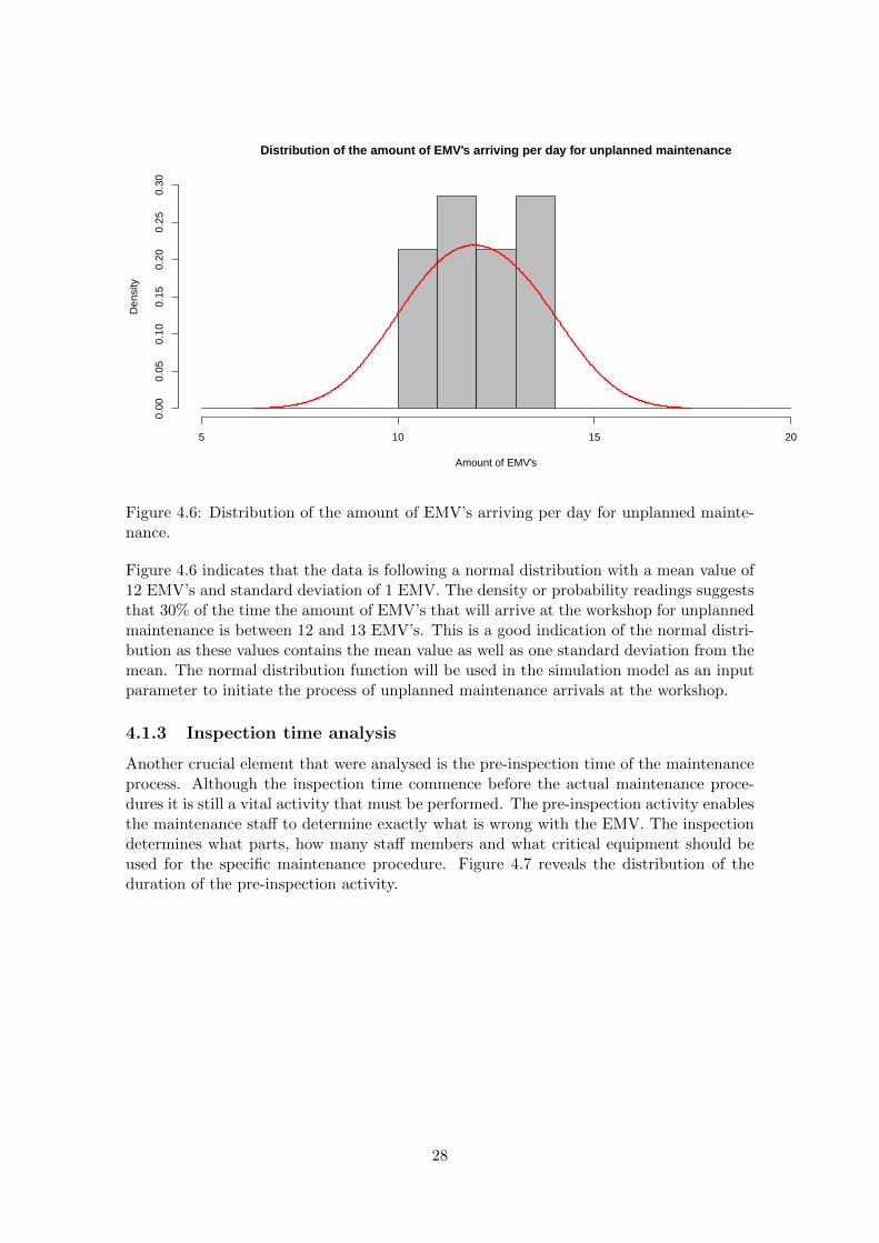
Figure 4.6 indicates that the data is following a normal distribution with a mean value of12 EMV’s and standard deviation of 1 EMV. The density or probability readings suggeststhat 30% of the time the amount of EMV’s that will arrive at the workshop for unplannedmaintenance is between 12 and 13 EMV’s. This is a good indication of the normal distri-bution as these values contains the mean value as well as one standard deviation from themean. The normal distribution function will be used in the simulation model as an inputparameter to initiate the process of unplanned maintenance arrivals at the workshop.

4.1.3 Inspection time analysis

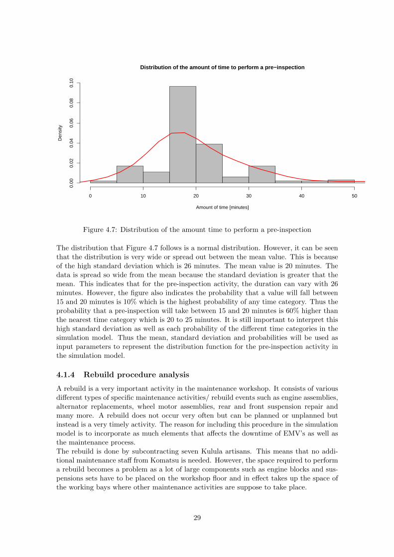
Another crucial element that were analysed is the pre-inspection time of the maintenanceprocess. Although the inspection time commence before the actual maintenance proce-dures it is still a vital activity that must be performed. The pre-inspection activity enablesthe maintenance staff to determine exactly what is wrong with the EMV. The inspectiondetermines what parts, how many staff members and what critical equipment should beused for the specific maintenance procedure. Figure 4.7 reveals the distribution of theduration of the pre-inspection activity.

28

Distribution of the amount of time to perform a pre−inspection


Den

sity

0 10 20 30 40 50

0.00

0.02

0.04

0.06

0.08

0.10

Figure 4.7: Distribution of the amount time to perform a pre-inspection

The distribution that Figure 4.7 follows is a normal distribution. However, it can be seenthat the distribution is very wide or spread out between the mean value. This is becauseof the high standard deviation which is 26 minutes. The mean value is 20 minutes. Thedata is spread so wide from the mean because the standard deviation is greater that themean. This indicates that for the pre-inspection activity, the duration can vary with 26minutes. However, the figure also indicates the probability that a value will fall between15 and 20 minutes is 10% which is the highest probability of any time category. Thus theprobability that a pre-inspection will take between 15 and 20 minutes is 60% higher thanthe nearest time category which is 20 to 25 minutes. It is still important to interpret thishigh standard deviation as well as each probability of the different time categories in thesimulation model. Thus the mean, standard deviation and probabilities will be used asinput parameters to represent the distribution function for the pre-inspection activity inthe simulation model.

4.1.4 Rebuild procedure analysis

A rebuild is a very important activity in the maintenance workshop. It consists of variousdifferent types of specific maintenance activities/ rebuild events such as engine assemblies,alternator replacements, wheel motor assemblies, rear and front suspension repair andmany more. A rebuild does not occur very often but can be planned or unplanned butinstead is a very timely activity. The reason for including this procedure in the simulationmodel is to incorporate as much elements that affects the downtime of EMV’s as well asthe maintenance process.The rebuild is done by subcontracting seven Kulula artisans. This means that no addi-tional maintenance staff from Komatsu is needed. However, the space required to performa rebuild becomes a problem as a lot of large components such as engine blocks and sus-pensions sets have to be placed on the workshop floor and in effect takes up the space ofthe working bays where other maintenance activities are suppose to take place.

29

There are different rebuild events that can take place. The different rebuild events alongwith the average amount of time it takes to complete can be seen in Table 4.2.

Table 4.2: Different rebuild events.Event description Average event duration [hours] Number of components Planned

LH and RH wheelmotor 100.25 2 Yes

Major rebuild - 25000 534.98 18 Yes

Engine change out 452.8 6 Yes

Major rebuild 321.5 13 Yes

Truck rebuild 782.37 17 Yes

Major rebuild and engine midlife - 25000 413.41 20 Yes

Rebuilds are typically planned with only 2.5% being unplanned. Table 4.2 indicates theaverage amount of time it will take to complete a specific rebuild event. For example, themajor rebuild occuring at 25000 operating hours for an EMV will usually take 535 hourswith 18 components to repair and the event was planned. This example can be used tointerpret the rest of the different events. In the simulation model these duration’s of thedifferent rebuild events will be incorporated to make the model as accurate as possible.

30

Chapter 5

Simulation model

A discrete-event simulation model was developed based on the statistical parameters andcharacteristics of the Komatsu maintenance workshop. The conceptual model describedby Duffuaa et al. (2001) in Chapter 3.1 was used as a guideline in developing the simu-lation model. Alterations were made to the conceptual model in order to incorporate theworkshop process as accurate as possible. The actual computer based simulation modelcan be seen in Appendix A. The objective of this simulation model is to imitate the cur-rent workshop process as accurate to the real system as possible in order to determinekey areas that contribute in excessive downtime (bottlenecks) and potential inefficiency ofmaintenance procedures.Different scenarios were created in the simulation. Scenarios such as increasing the stan-dard times to perform certain maintenance activities, adding one more operating bay forincreased work space and analysing the efficiency of the maintenance procedures were in-vestigated. The change in downtimes and efficiency were measured per scenario to obtaininformation as to where an opportunity of improvement exists in the workshop.The model validation was done by comparing the model outputs to the real maintenanceprocess outputs. The validation of the model is a crucial step that must be performedin order to determine the accuracy to which the model simulates the current workshopprocess and evidently generate useful results.

5.1 Maintenance process flow

The simulation model was designed according to the current process flow of the mainte-nance workshop. It is important to first understand the basic activities that makes up theprocess flow. A simple schematic sketch can be seen in Figure 5.1 of the current processflow within the workshop.

31

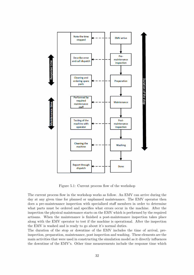
Figure 5.1: Current process flow of the workshop

The current process flow in the workshop works as follow. An EMV can arrive during theday at any given time for planned or unplanned maintenance. The EMV operator thendoes a pre-maintenance inspection with specialized staff members in order to determinewhat parts must be ordered and specifies what errors occur in the machine. After theinspection the physical maintenance starts on the EMV which is performed by the requiredartisans. When the maintenance is finished a post-maintenance inspection takes placealong with the EMV operator to test if the machine is operational. After the inspectionthe EMV is washed and is ready to go about it’s normal duties.The duration of the stop or downtime of the EMV includes the time of arrival, pre-inspection, preparation, maintenance, post inspection and washing. These elements are themain activities that were used in constructing the simulation model as it directly influencesthe downtime of the EMV’s. Other time measurements include the response time which

32

includes only the pre-maintenance inspection and preparation. The maintenance timemeasurement includes only the maintenance and post-inspection of the EMV’s.The current process flow of the workshop were also used to identify the areas where thedata gathering was done described in Chapter 4.

5.2 Model interpretation

The simulation model was constructed using Figure 5.1 as a basic guideline for the con-struction of the simulation model as well as the conceptual model design. The first partof the simulation model consists of the arrival rate and inspection time which can begrouped as the arrival module. The second part consists of the maintenance time andpost-maintenance inspection time which can be grouped as the maintenance module. Thelast part of the simulation model consists of the washing and cleaning time which can begrouped as the washing module. These different processes were divided into the specificmodules in order to help develop the simulation model and understand the complexity ofthe workshop.

5.2.1 Simulation of arrival module

The arrival module consists of a number of elements. These elements include the plannedand unplanned arrival rates and inspection times of the EMV’s. The simulation modelexecutes the arrival module in discrete time events. The model starts with a source whichrepresents the planned and unplanned arrival rates for the EMV’s. The data from Section4.1.1 and Section 4.1.2 were used as the arrival rates in the simulation model. Once theEMV has arrived at the workshop either as a planned or unplanned entity it is theninspected to determine what type of maintenance must be done. The model uses a delayto represent the inspection element and incorporates the inspection time obtained fromthe data analysis in Section 4.1.3 as an input parameter. After the execution of each eventin the arrival module the simulation model moves on to the maintenance module.

5.2.2 Simulation of the maintenance module

The maintenance model consists of a number of elements. These elements include thedifferent maintenance procedures and the post-maintenance inspection time. The variousmaintenance procedures are incorporated in the simulation model by using the respectedprobabilities and distribution functions as described in Chapter 4.1. In order to incorporatethese different maintenance procedures with their respective statistics the model uses anobject that routes the planned EMV to a port given the probability it occurs and forhow long it endures the specific maintenance procedure. This mechanism incorporatesthe crucial elements in the workshop and is very useful in the simulation model. Afterthe completion of the specific maintenance procedure the model moves towards the post-maintenance inspection object. This object simulates the amount of time any given EMVspends in the post-maintenance inspection phase. The simulation model uses a delayobject to simulate this event and in effect delay/ pause the process in order to incorporatethe time an EMV will spend in post-maintenance inspection. The maintenance module canbe considered as the most important focus point in the simulation model as it representsthe different kinds of maintenance procedures which contributes the most to downtime inEMV’s. After the model has executed the events of the maintenance module, it moves onto the washing module.

33

5.2.3 Simulation of the washing module

The washing module consists of washing and cleaning of the EMV after all the abovementioned modules have been executed in the simulation model. This module is also veryimportant as it contributes to the overall downtime of the EMV’s. The model interpretsthis event by using a delay object. After the washing is complete the EMV exits themaintenance workshop area and thus complete the maintenance process. This is alsowhere the simulation model stops.

5.3 Model validation

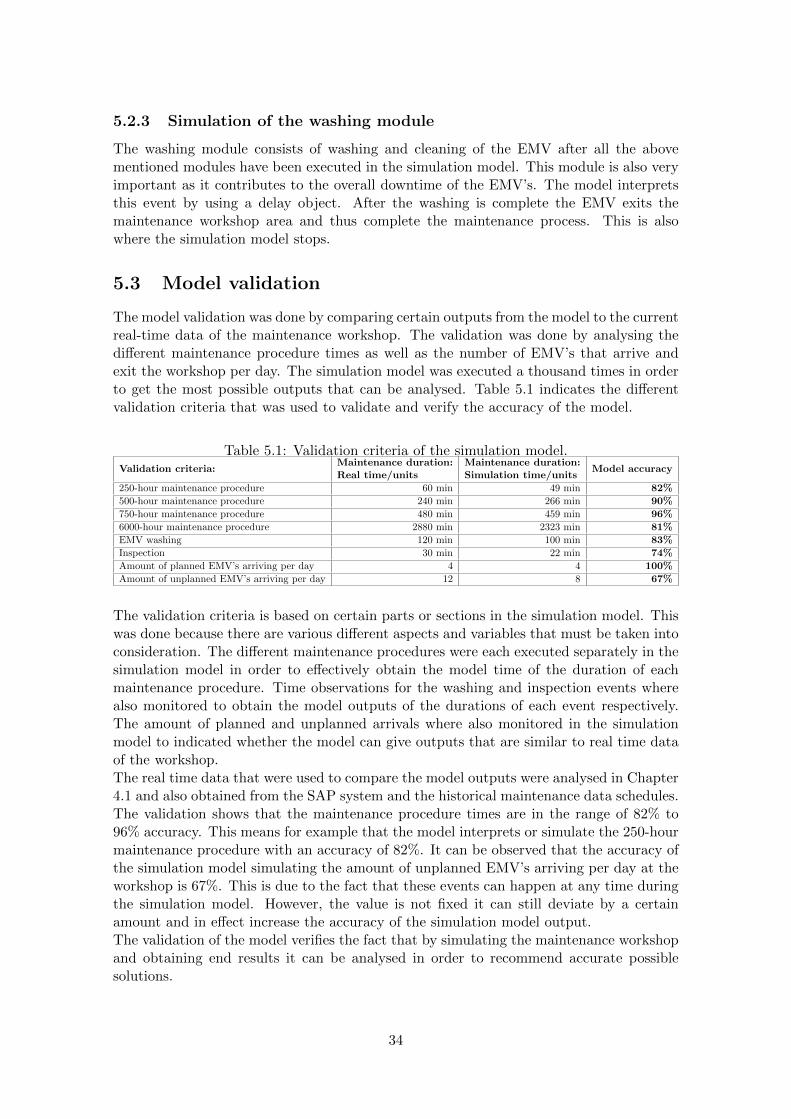
The model validation was done by comparing certain outputs from the model to the currentreal-time data of the maintenance workshop. The validation was done by analysing thedifferent maintenance procedure times as well as the number of EMV’s that arrive andexit the workshop per day. The simulation model was executed a thousand times in orderto get the most possible outputs that can be analysed. Table 5.1 indicates the differentvalidation criteria that was used to validate and verify the accuracy of the model.

Table 5.1: Validation criteria of the simulation model.Validation criteria:

Maintenance duration:Real time/units

Maintenance duration:Simulation time/units

Model accuracy

250-hour maintenance procedure 60 min 49 min 82%




EMV washing 120 min 100 min 83%

Inspection 30 min 22 min 74%

Amount of planned EMV’s arriving per day 4 4 100%

Amount of unplanned EMV’s arriving per day 12 8 67%

The validation criteria is based on certain parts or sections in the simulation model. Thiswas done because there are various different aspects and variables that must be taken intoconsideration. The different maintenance procedures were each executed separately in thesimulation model in order to effectively obtain the model time of the duration of eachmaintenance procedure. Time observations for the washing and inspection events wherealso monitored to obtain the model outputs of the durations of each event respectively.The amount of planned and unplanned arrivals where also monitored in the simulationmodel to indicated whether the model can give outputs that are similar to real time dataof the workshop.The real time data that were used to compare the model outputs were analysed in Chapter4.1 and also obtained from the SAP system and the historical maintenance data schedules.The validation shows that the maintenance procedure times are in the range of 82% to96% accuracy. This means for example that the model interprets or simulate the 250-hourmaintenance procedure with an accuracy of 82%. It can be observed that the accuracy ofthe simulation model simulating the amount of unplanned EMV’s arriving per day at theworkshop is 67%. This is due to the fact that these events can happen at any time duringthe simulation model. However, the value is not fixed it can still deviate by a certainamount and in effect increase the accuracy of the simulation model output.The validation of the model verifies the fact that by simulating the maintenance workshopand obtaining end results it can be analysed in order to recommend accurate possiblesolutions.

34

Chapter 6

Results and recommendations

The simulation model was executed for different scenarios, changing some parameters inthe model in order to determine areas which contributes to excessive downtime of theEMV’s as well as inefficient activities. The different scenarios were formulated accordingto the current data analysis as well as information gathered from the Komatsu supervisorsas to where they think possible problems occur that contribute to inefficient practices andunnecessary downtime of the EMV’s. The different scenarios include the following.

1. Increasing the amount of operating bays.

2. Changing the amount of workers per maintenance procedure.

3. Measuring the time efficiency of maintenance procedures.

6.0.1 Increasing the amount of operating bays

The workshop is currently using four of the five operating bays for pure maintenanceprocedures. The other operating bay is used for temporary storage of the big componentswhen and EMV undergoes maintenance. This results in the workshop having one lessoperating bay to perform possible maintenance procedures. In the simulation model theeffect of changing the number of operating bays from 1 through to 10 were observed. Themodel indicated that if the operating bay were to be changed to either one, two or three,a 0% time reduction will occur. By increasing the amount of operating bays from fourto five, a 20% reduction in downtime was observed from the simulation model. Although20% seems small it is in fact a very large proportion of downtime reduction in the overallmaintenance process. Table 6.1 indicates the percentage time reductions of the differentamount of operating bays.

35

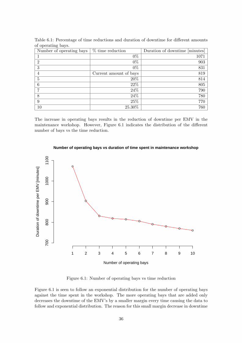
Table 6.1: Percentage of time reductions and duration of downtime for different amountsof operating bays.

Number of operating bays % time reduction Duration of downtime [minutes]

1 0% 1071

2 0% 903

3 0% 831

4 Current amount of bays 819

5 20% 814

6 22% 805

7 24% 790

8 24% 780

9 25% 770

10 25.30% 760

The increase in operating bays results in the reduction of downtime per EMV in themaintenance workshop. However, Figure 6.1 indicates the distribution of the differentnumber of bays vs the time reduction.

700

800

900

1000

1100

Number of operating bays vs duration of time spent in maintenance workshop

Number of operating bays

Dur

atio

n of

dow

ntim

e pe

r E

MV

[min

utes

]

1 2 3 4 5 6 7 8 9 10

Figure 6.1: Number of operating bays vs time reduction

Figure 6.1 is seen to follow an exponential distribution for the number of operating baysagainst the time spent in the workshop. The more operating bays that are added onlydecreases the downtime of the EMV’s by a smaller margin every time causing the data tofollow and exponential distribution. The reason for this small margin decrease in downtime

36

is because of the utilisation of workers. When there are more bays more work has to bedone and in effect increases the utilisation of workers to such an extent that they struggleto keep up with maintenance schedules.

6.0.2 Changing the amount of workers per maintenance procedure

The different maintenance procedures described in Section 4.1.1 each have a unique numberof artisans assigned to a different maintenance procedure. The simulation model wasused to gather the current information regarding the worker utilisation per maintenanceprocedure as well as changing the amount of workers and observing the effect of the workerutilisation. The current worker utilisation were analysed first in order to determine whichmaintenance processes are over utilised. After analysing the utilisation of the workforceper maintenance procedure it was observed that some of the procedures were performedeffectively in terms of worker utilisation and some procedures over utilised the workforce.Table 6.2 indicates the utilisation of workers of the different maintenance procedures.

Table 6.2: Utilisation of workers at different maintenance procedures.Maintenance procedures Amount of workers required Worker utilisation

250-hour 1 57%

500-hour 1 84%

750-hour 5 95%

6000-hour 5 95%

37

The 250-hour maintenance procedure indicates that only 57% of the workforce is beingutilised for this procedure. This is understandable as the 250-hour procedure only requiresone artisan to execute the maintenance procedure. The 500-hour maintenance procedure isat a respected 84% utilisation which is acceptable for this kind of maintenance procedure asit also only requires one artisan. The use of the simulation model for these two maintenanceprocedures were to only determine the worker utilisation. These two procedures are alreadyutilised effectively so it was not necessary to change the amount of workers and analysedthe effect from the simulation model.The 750-hour and 6000-hour maintenance procedures indicated that 95% of the workforceis being utilised. This utilisation of the workforce is unnecessarily high and must be re-duced. The maintenance time and number of activities that must be performed on each ofthese procedures are very high which causes the high workforce utilisation. Both of theseprocedures require atleast five skilled artisans to perform the maintenance. The simula-tion model were used to change the amount of workers for each respective maintenanceprocedure. Table 6.3 indicates the change in worker utilisation for the 750-hr and 6000-hrmaintenance procedures for different amount of workers.

Table 6.3: Change in worker utilisation for the 750-hr and 6000-hr maintenance proceduresfor different amount of workers.

Maintenance procedures Amount of workers Worker utilisation

750-hour 5 95%

6 76%

7 59%

6000-hour 5 95%

6 70%

7 59%

The increase of one worker (to six) for the 750-hr maintenance procedure decreased theworker utilisation from 95% to 76%. This increase of one more worker indicated that theworker utilisation for the 750-hr maintenance procedure can be reduced to a reasonableand effective worker utilisation. However, by increasing the number of workers to seven itwas observed that the worker utilisation only decreased by a marginal amount. Thus itwas concluded that for the 750-hr maintenance procedure a optimal amount of 6 workersmust be available to perform the maintenance activities.The 6000-hr maintenance procedure also indicated a change in worker utilisation afterchanging the amount of workers in the simulation model. The simulation model resultsindicated that by increasing the amount of workers to six a decrease (from 95% to 70%)of 25% in worker utilisation was observed. The change in worker utilisation to 70% is arespectable worker utilisation for the maintenance procedure and it is recommended thatthe workshop hire one more worker for the 6000-hr maintenance procedure as well.For both of these procedures it is recommended that if the management of the workshopwishes to implement more than five workers per maintenance procedure, they must takeinto account the cost associated to hire more workers.These two maintenance procedures are seen as areas of improvement and it is recommendedthat the workshop investigate this matter in order to appoint more artisans that canexecute these maintenance procedures.

38

6.0.3 Efficiency of maintenance procedures

The efficiency of the different maintenance procedures were gathered from the simulationmodel in order to determine areas for improvement.The maintenance procedure efficienciesas well as the workforce utilisation, as seen in Table 6.2, were analysed. It was importantto observe the efficiency along with the workforce utilisation as both of these outputsinterrelate with one another. The efficiency of the maintenance procedures were calculatedusing formula 6.1.

Efficiency =SLH

ATW× 100 (6.1)

Where SLH = standard labour hours and ATW = actual time worked.The standard labour hours were obtained from previous data from the workshop and theactual time worked relates to the different outputs gathered from the simulation model.Table 6.4 indicates the efficiency measurements on the different maintenance proceduresalong with the worker utilisation results gathered in Table 6.2.

Table 6.4: Efficiency measurements of the different maintenance proceduresMaintenance procedure Standard time Actual time Efficiency Worker utilisation

250-hour 60 min 46 min 130% 57%

500-hour 240 min 190 min 126% 84%

750-hour 480 min 613 min 78% 95%

6000-hour 2880 min 1172 min 246% 95%

At first it was observed that the 250-hour, 500-hour and 6000-hour maintenance proce-dures had efficiencies greater than 100%. This indicated that the actual time observedfrom the simulation model for each of these procedures were less than the standard timeproposed by the historical maintenance data. Although this seams as a good indicationof efficient maintenance procedures it is also important to look at the worker utilisationalong with the efficiency. The efficiency of the 250-hour maintenance procedure indicatedthat it is 130% efficient with a worker utilisation of 57%. This procedure is being executedefficiently and no opportunity for improvement exist.The efficiency of the 750-hour maintenance procedure indicated that it is 78% efficientwith a worker utilisation of 95%. The high worker utilisation suggested that all of therequired workforce needed for this maintenance procedure is being used to only achieve a78% efficiency. This meant that the actual time to perform the maintenance activity tooklonger than the standard time. This resulted in an increase in downtime for EMV’s and ineffect established an area for improvement. Increasing the workforce for this maintenanceprocedure by one artisan decreased the worker utilisation to 76% and increased the effi-ciency to 87%. This recommended solution seems promising, although the cost analysisof hiring one more worker does not fall within the scope of this project it must be takeninto consideration as cost always plays an important role in any organisation.

39

Chapter 7

Conclusion

This report describes and outlines the current problems that exists in the maintenanceworkshop as well as the need to measure efficiencies to establish potential bottlenecks.Through investigating the workshop first hand and by implementing industrial techniquessuch as statistical data analysis, simulation modeling, system analysis as well as systemsengineering, a problem background, literature study and conceptual model were formu-lated. Using the information and literature gathered in these chapters a computer basesimulation model was developed in order to accurately identify areas of improvement inthe maintenance workshop.The respected parameters that were obtained from the statistical analysis in Chapter 4enabled the user to accurately incorporate the main activities that are executed in theworkshop. After validating each section of the model different scenarios were analysed toidentify key improvement areas.It was found that by increasing the number of operating bays in the maintenance workshopa reduction in downtime of EMV’s were observed from the model outputs. This area clearlyindicated an opportunity for improvement.Analysing the worker utilisation and changing the amount of workers per maintenance pro-cedure indicated another area for improvement. Both the 750-hr and 6000-hr maintenanceprocedures decreased their worker utilisation by increasing the number of workers to six.The 750-hour maintenance procedure was established to be less efficient with an abnor-mal high workforce utilisation. Increasing the work force for this maintenance procedureresulted in an increase in efficiency of the maintenance procedure as well.These three areas were identified in being areas that contribute to the excessive downtimeand in-efficient workshop practices. By implementing the recommendations and investigat-ing these areas more in depth it can be assured that the Komatsu maintenance workshopwill increase the efficiency of maintenance practices and in effect decrease the amount ofdowntime for EMV’s.

40

Bibliography

Abdulnour, G., Dudek, R., and Smith, M. (1995). Effect of maintenance policies onthe just-intime production system. International Journal of Production Research,,33(2):565–583.

Alabdulkarim, E., Ball, P., and Tiwari, A. (2015). Assessing asset monitoring levels formaintenance operations: A simulation approach. Journal of Manufacturing TechnologyManagement, pages 632–659.

Ali, A., Chen, X., and Yang, Z. (2008). Optimized maintenance design for manufacturingperformance improvement using simulation. In Proceeding of 2008 Winter SimulationConference, Institute of Electrical and Electronics Engineers Inc., pages 1811–1891.

Andriulo, S., Arleo, M., and de Carlo, F. (2015). Effectiveness of maintenance ap-proaches for high reliability organizations. International Federation of AutomaticControl, 48(8):466–471.

Baldwin, C., Sauser, B., and Cloutier, R. (2015). 2015 conference on systems engi-neering research. In Inc., E., editor, Simulation Approaches for System of Systems:Events-Based versus Agent Based Modeling, volume 44, pages 363–372. Procedia Com-puter Science, Elsevier B.V.

Bonabeau, E. (2002). Agent-based modeling: Methods and techniques for simulatinghuman systems. 99:7280–7287.

Duffuaa, S., Ben-Daya, M., and Al-Sutan, K. (2001). A generic conceptual simula-tion model for maintenance systems. Journal of Quality in Maintenance Engineering,7(3):207–219.

Grall, A., Berenguer, C., and Dieulle, L. (2002). A condition-based maintenance policy forstochastically deteriorating systems. Reliable Engineering and System Safety, 76(2):167–180.

Greasley, A. (2000). Using simulation to assess the service reliability of a train maintenancedepot. Quality Reliability Engineering International, 16(3):221–228.

Gulati, R. and Smith, R. (2009). Maintenance and Reliability Best Practices. IndustrialPress Inc.

Joo, S., Levary, R., and Ferris, M. (1997). Planning preventative maintenance for a fleetof police vehicles using simulation. Simulation, 68:93–100.

Keith, R. and Smith, R. (2008). Rules of Thumb for Maintenance and ReliabilityEngineers. Elsevier Inc.

41

Lavoie, P., Navarra, P., and Kuhne, R. (2009). Dynamic simulation in iron ore pelletisingplants. Technical report, Australasian Institute of Mining and Metallurgy.

Lightfoot, H., Baines, T., and Smart, P. (2011). Examining the information and com-munication technologies enabling servitized manufacture. Proceedings of the Instituteof Mechanical Engineers Part B: Journal of engineering manufacture Vol. 225 No. 10,pages 1964–1968.

Mattila, V., Virtanen, K., and Raivo, T. (2008). Improving maintenance decision makingin the finnish air force through simulation. Interfaces, 38(3):187–201.

Mosley, A., Teyner, T., and Uzsoy, R. (1998). Maintenance scheduling and staffing policiesin a wafer fabriction facility. IEEE Transactions on Wafer manufacturing, 11:316–323.

Noemi, M. and Leigh, W. (1993). Maintenance scheduling: Issues, results and researchneeds. International Journal of Operations and Production Management, 14:47–69.

Pannirselvam, G., Ferguson, L., and Ash, R. (1999). Operations management research:an update for the 1990’s. Journal of Operations Management, 18(1):95–112.

Petersen, K., Khurum, M., and Lefteris, A. (2014). Reasons for bottlenecks in very large-scale system of systems development. Information and Software Technology, 54:1403–1420.

Resonant (2017). About us. www.resonant.co.za.

Savsar, M. (1990). Maintenance crew size determination by computer simulation. InRiyadh, editor, First Scientific Symposium on Maintenance, Planning and Operations,pages 95–108.

Smith, R. (2004). Best maintenance practices. Lean Maintenance, pages 219 –263.

Tiwari, A. and Alrabghi, A. (2016). A novel approach for modelling complex maintenancesystems using discrete event simulation. Reliability Engineering and System Safety,154:160–170.

42

Appendices

43

Appendix A

Planning scheduling element

44

Figure A.1: Planning and scheduling element

45

Appendix B

Computer-based simulation model

46

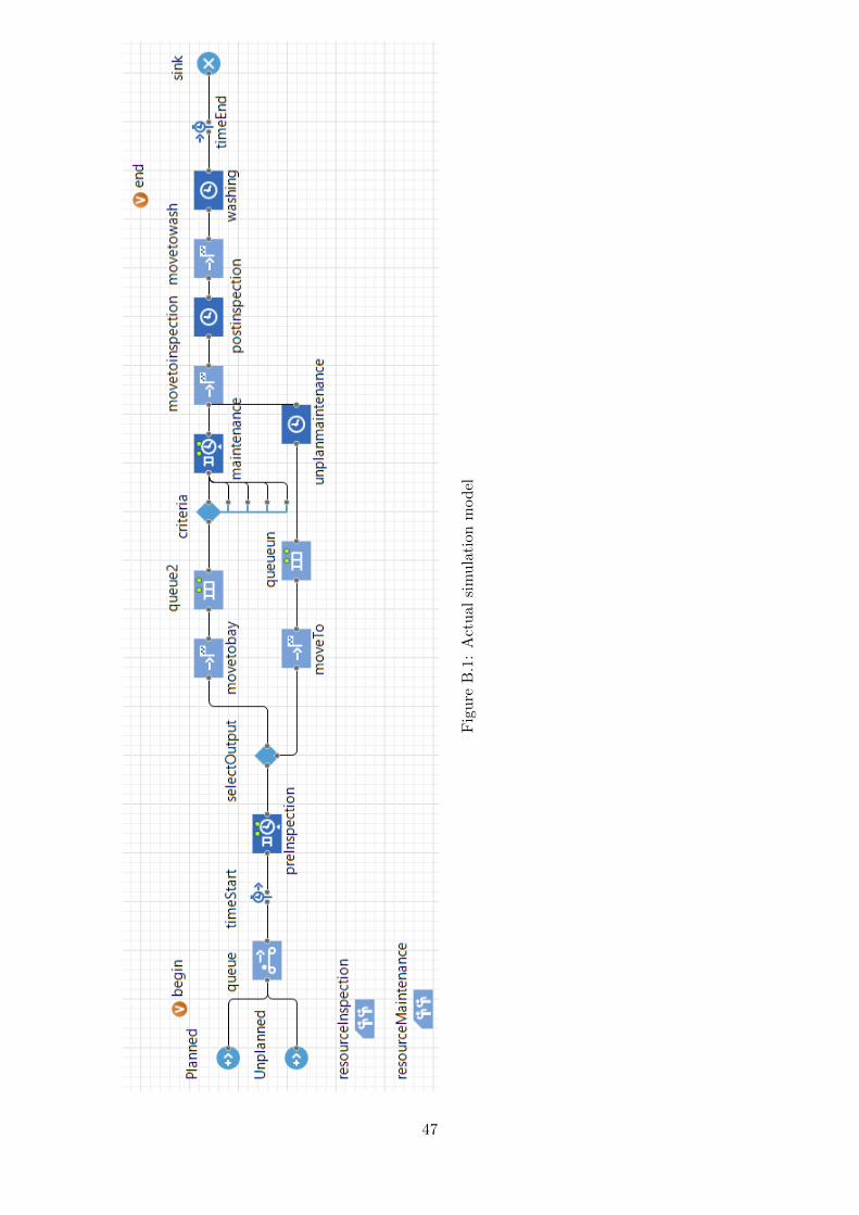
Fig

ure

B.1

:A

ctu

alsi

mu

lati

onm

od

el

47

Appendix C

Sponsorship form

48

Department of Industrial & Systems Engineering

Final Year Projects

Identification and Responsibility of Project Sponsors

All Final Year Projects are published by the University of Pretoria on UPSpace and thus freely available

on the Internet. These publications portray the quality of education at the University and have the

potential of exposing sensitive company information. It is important that both students and company

representatives or sponsors are aware of such implications.

Key responsibilities of Project Sponsors:

A project sponsor is the key contact person within the company. This person should thus be able to

provide the best guidance to the student on the project. The sponsor is also very likely to gain from

the success of the project. The project sponsor has the following important responsibilities:

1. Confirm his/her role as project sponsor, duly authorised by the company. Multiple sponsors

can be appointed, but this is not advised. The duly completed form will considered as

acceptance of sponsor role.

2. Review and approve the Project Proposal, ensuring that it clearly defines the problem to be

investigated by the student and that the project aim, scope, deliverables and approach is

acceptable from the company’s perspective.

3. Review the Final Project Report (delivered during the second semester), ensuring that

information is accurate and that the solution addresses the problems and/or design

requirements of the defined project.

4. Acknowledges the intended publication of the Project Report on UP Space.

5. Ensures that any sensitive, confidential information or intellectual property of the company is

not disclosed in the Final Project Report.

Project Sponsor Details:

Company: Resonant Industrial (Pty) Ltd (in co-operation with Anglo Platinum Mines)

Project Description: Simulation and measurement of the activities in a maintenance workshop

at Anglo Platinum Mines for mining trucks, to identify potential

bottlenecks.

Student Name: Francois MF Venter

Student number: 14118735

Student Signature: F.Venter

Sponsor Name: Abraham Groenewald

Designation: Director

E-mail: [email protected]

Tel No: 012 665 1109

Cell No: 082 55 44 242

Fax No: -

Signature:

49

using a discrete -event simulation model to identify

Documents