discrete event simulation with ... - home - springer · discrete event simulation with application...

DISCRETE EVENT SIMULATION WITHAPPLICATION TO COMPUTERCOMMUNICATION SYSTEMS PERFORMANCEIntroduction to Simulation

Helena Szczerbicka1, Kishor S. Trivedi2 and Pawan K. Choudhary2

1University of Hannover, Germany ; 2Duke University, Durham, NC

Abstract: As complexity of computer and communication systems increases, it becomes hardto analyze the system via analytic models. Measurement based systemevaluation may be too expensive. In this tutorial, discrete event simulation as amodel based technique is introduced. This is widely used for theperformance/availability assessment of complex stochastic systems.Importance of applying a systematic methodology for building correct,problem dependent, and credible simulation models is discussed. These will bemade evident by relevant experiments for different real-life problems andinterpreting their results. The tutorial starts providing motivation for usingsimulation as a methodology for solving problems, different types ofsimulation (steady state vs. terminating simulation) and pros and cons ofanalytic versus simulative solution of a model. This also includes differentclasses of simulation tools existing today. Methods of random deviategeneration to drive simulations are discussed. Output analysis, involvingstatistical concepts like point estimate, interval estimate, confidence intervaland methods for generating it, is also covered. Variance reduction and speed-up techniques like importance sampling, importance splitting and regenerativesimulation are also mentioned. The tutorial discusses some of the most widelyused simulation packages like OPNET MODELER and ns-2. Finally thetutorial provides several networking examples covering TCP/IP, FTP andRED.

Key words: Simulation, Statistical Analysis, random variate, TCP/IP, OPNET MODELERand ns-2

In many fields of engineering and science, we can use a computer tosimulate natural or man-made phenomena rather than to experiment with thereal system. Examples of such computer experiments are simulation studiesof congestion control in a network and competition for resources in a

272 Helena Szczerbicka, Kishor S. Trivedi and Pawan K. Choudhary

computer operating system. A simulation is an experiment to determinecharacteristics of a system empirically. It is a modeling method that mimicsor emulates the behavior of a system over time. It involves generation andobservation of artificial history of the system under study, which leads todrawing inferences concerning the dynamic behavior of the real system.

A computer simulation is a discipline of designing a model of an actualor theoretical system, executing the model (an experiment) on a digitalcomputer, and statistically analyzing the execution output (see Fig. 1). Thecurrent state of the physical system is represented by state variables(program variables). Simulation program modifies state variables toreproduce the evolution of the physical system over time.

This tutorial provides an introductory treatment of various conceptsrelated to simulation. In Section 1 we discuss the basic notion of going fromthe system description to its simulation model. In Section 2, we provide abroad classification of simulation models followed by a classification ofsimulation modeling tools/languages in Section 3. In Section 4 we discussthe role of probability and statistics in simulation while in Section 5 wedevelop several networking applications using the simulation tools OPNETMODELER and ns-2. Finally, we conclude in Section 6.

1. FROM SYSTEM TO MODEL

System can be viewed as a set of objects with their attributes andfunctions that are joined together in some regular interaction toward theaccomplishment of some goal. Model is an abstract representation of asystem under study. Some commonly used model types are:

Analytical Models. These employ mathematical formal descriptions likealgebraic equations, differential equations or stochastic processes andassociated solution procedures to solve the model. For examplecontinuous time Markov chains, discrete time Markov chains, semi-Markov and Markov regenerative models have been used extensively forstudying reliability/availability/performance and performability ofcomputer and communication systems [1].

Closed form Solutions: Underlying equations describing the dynamicbehavior of such models can sometimes be solved in closed form if themodel is small in size (either by hand or by such packages asMathematica) or if the model is highly structured such as the Markovchain underlying a product-form queuing network [1].Numerical Methods: When the solution of an analytic model cannot beobtained in a closed form, then computational procedures are used to

1.

1.

2.

Discrete event simulation with application to computer communicationsystems performance

273

numerically solve analytical models using packages such as SHARPE[2] or SPNP [3]

Simulation models: Employ methods to “run” the model so as to mimicthe underlying system behavior; no attempt is made to solve the equationsdescribing system behavior as such equations may be either too complexor not possible to formulate. An artificial history of the system understudy is generated based on model assumptions. Observations arecollected and analyzed to estimate the dynamic behavior of the systembeing simulated. Note that simulation provides a model-based evaluationmethod of system behavior but it shares its experimental nature withmeasurement-based evaluation and as such needs the statistical analysis of

2.

its outputs.

Figure 1. Simulation based problem solving

Simulation or analytic models are useful in many scenarios. As the realsystem becomes more complex and computing power becomes faster andcheaper, modeling is being used increasingly for the following reasons [4]:

If the system is unavailable for measurement the only option available forits evaluation is to use a model. This can be the case if system is beingdesigned or it is too expensive to experiment with the real systemEvaluation of system under wide variety of workloads and network types(or protocols).

1.

2.


Suggesting improvement in the system under investigation based onknowledge gained during modeling.Gaining insight into which variables are most important and howvariables interact.New polices, decision rules, information flows can be explored withoutdisrupting ongoing operations of the real system.New hardware architectures, scheduling algorithms, routing protocols,reconfiguration strategies can be tested without committing resources fortheir acquisition/implementation.

While modeling has proved to be a viable and reliable alternative tomeasurements on the real system, the choice between analytical andsimulation is still a matter of importance For large and complex systems,analytic model formulation and/or solution may require making unrealisticassumptions and approximations. For such systems simulation models canbe easily created and solved to study the whole system more accurately.Nevertheless, many users often employ simulation where a faster analyticmodel would have served the purpose.

Some of difficulties in application of simulation are:Model building requires special training. Frequently, simulation

languages like Simula [5], Simscript [6], Automod [7], Csim [8], etc areused. Users need some programming expertise before using theselanguages.Simulation results are difficult to interpret, since most simulation outputs

are samples of random variables. However most of the recent simulationpackages have inbuilt output analysis capabilities to statistically analyzethe outputs of simulation experiments.Though the proper use of these tools requires a deep understanding

statistical methods and necessary assumptions to assert the credibility ofobtained results. Due to a lack of understanding of statistical techniquesfrequently simulation results can be wrongly interpreted [9].Simulation modeling and analysis are time consuming and expensive.

With availability of faster machines, development in parallel anddistributed simulation [10, 11] and in variance reduction techniques suchas importance sampling [12, 13, 14], importance splitting [15, 16, 17] andregenerative simulation [18], this difficulty is being alleviated.

In spite of some of the difficulties, simulation is widely used in practice andthe use of simulation will surely increase manifold as experimenting withreal systems gets increasingly difficult due to cost and other reasons. Henceit is important for every computer engineer (in fact, any engineer) to befamiliar with the basics of simulation.

3.

4.

5.

6.

1.

2.

3.

4.


275

2. CLASSIFICATION OF SIMULATION MODELS

Simulation models can be classified according to several criteria [19]:Continuous vs. Discrete: Depending upon the way in which statevariables of the modeled system change over time. For exampleconcentration of a substance in a chemical reactor changes in a smooth,continuous fashion like in a fluid flow whereas changes in the length of aqueue in a packet switching network can be tracked at discrete points intime. In a discrete event simulation changes in the modeled state variableare triggered by scheduled events [20].Deterministic vs. stochasticThis classification refers to type of variables used in the model beingsimulated. The choice of stochastic simulation makes it experimental innature and hence necessitates statistical analysis of results.Terminating vs. Steady state: A terminating simulation is used to studythe behavior of a system over a well-defined period of time, for examplefor the reliability analysis of a flight control system over a designatedmission time. This corresponds to transient analysis put in the context ofanalytic models. Whereas steady state simulation corresponds to thesteady state analysis in the context of analytic models. As such, we haveto wait for the simulation system output variables to reach steady statevalues. For example, the performance evaluation of a computer ornetworking system is normally (but not always) is done using steady statesimulation. Likewise, the availability analysis is typically carried out forsteady state behavior.Synthetic or distribution driven vs. Trace driven: A time-stampedsequence of input events is required to drive a simulation model. Such anevent trace may already be available to drive the simulation hencemaking it a trace driven simulation. Examples are cache simulations forwhich many traces are available. Similarly, traces of packet arrival events(packet size, etc.) are first captured by using a performance measurementtool such as tcpdump. Then these traces are used as input traffic to thesimulation. Lots of traces are freely available on Web. One of Internettraces archive is http://ita.ee.lbl.gov. Alternatively, event traces can besynthetically generated. For the synthetic generation, distributions of allinter-event times are assumed to be known or given and then randomdeviates of the corresponding distributions are used as the time to nextevent of that type. We will show how to generate random deviates ofimportant distributions such as the exponential, the Weibull and thePareto distribution. The distribution needed to drive such distribution

1.

2.

3.

4.


5.

driven simulations may have been obtained by statistical inference basedon real measurement data.

Sequential vs. Distributed simulation: Sequential simulation processesevents in a non-decreasing time order. In distributed simulation a primarymodel is distributed over heterogeneous computers, which independentlyperform simulations locally. The challenge is to produce such a finaloverall order of events, which is identical with the order that would begenerated when simulating the primary model on a single computer,sequentially. There is extensive research in parallel and distributedsimulation [10,11].

The rest of this tutorial is concerned with sequential, distribution drivendiscrete event simulation.

3. CLASSIFICATION OF SIMULATION TOOLS

3.

1.

2.

Simulation tools can be broadly divided into three basic categories:General Purpose Programming Language (GPPL): - C, C++, Java aresome of the languages which have the advantage of being readilyavailable. These also provide a total control over software developmentprocess. But the disadvantage is that model construction takesconsiderable time. Also it doesn’t have support for any control of asimulation process. Furthermore, generation of random deviates forvarious needed distributions and the statistical analysis of output willhave to be learned and programmed.Plain Simulation Language (PSL) - SIMULA, SIMSCRIPT II.5 [6],SIMAN, GPSS, JSIM, SILK are some of the examples. Almost all ofthem have basic support for discrete event simulation. One drawback isthat they are not readily available. There is also the need forprogramming expertise in a new language.Simulation Packages (SPs)- like OPNET MODELER [21], ns-2 [22],CSIM [8], COMMNET III, Arena [23], Automod [7], SPNP [3] etc.They have a big advantage of being user-friendly, with some of themhaving graphical user interface. They provide basic support for discreteevent simulation (DES) and statistical analysis as well as severalapplication domains like TCP/IP networks. This ensures that modelconstruction time is shorter. Some simulation tools like OPNETMODELER also provide user an option of doing analytical modeling ofthe network. The negative side is that they are generally expensive,although most of them have free academic version for research. LikePSL, SPs require some expertise in new language/environment, and theytend to be less flexible than the PSLs.


277

Information about a variety of available simulation tools can be found at:http://www.idsia.ch/~andrea/simtools.html

4. THE ROLE OF STATISTICS IN SIMULATION

There are two different uses of statistical methods and one use ofprobabilistic methods in distribution driven simulations. First, thedistributions of input random variables such as inter-arrival times, times tofailure, service times, times to repair, etc. need to be estimated from realmeasurement data. Statistical inference techniques for parameter estimationand fitting distributions are covered in [1] and will be reviewed in thetutorial. Using random number generators, probabilistic methods ofgenerating random deviates are then used to obtain inter-event times anddrive the simulation. Once again this topic is covered in [1] and will bereviewed. Simulation runs are performed as computer experiments in orderto determine the characteristics of its output random variables. A singlesimulation run produces sample of values of an output variable over time.Statistical techniques are employed here to examine the data and to getmeaningful output from the experiment. Also they are used to define thenecessary length of simulation (the size of the sample), characteristics ofoutput variables like mean value and some assessments regarding anaccuracy of results. Two principal methods, independent replication and themethod of batch means, will be discussed.

In the following subsections we discuss random variate generationmethods and the statistical analysis of simulation output.

4.1 Random Variate generation

In this section we describe methods of generating random deviates of anyarbitrary distribution, assuming a routine to generate uniformly distributedrandom numbers is available. The distribution can be either continuous ordiscrete. Most of the simulation packages like OPNET MODELER, ns -2 andCSIM have built-in routines for generating random variates. But stillknowledge of random variate generation is necessary to more accuratelymodel the real world problem especially when available built-in generatorsin simulation packages do not support the needed distribution. Some of thepopular methods for generating variates are [1,4]:1. Inverse Transform: In this method the following property is used: if X is

a continuous random variable with the CDF F, than the new randomvariable Y=F(X) is uniformly distributed over the interval (0, 1). Thus to


generate a random deviate x of X first a random number u from a uniformdistribution over (0, 1) is generated and then the F is inverted.gives the required value of x. This can be used to sample fromexponential, uniform, Weibull, triangular, as well as empirical anddiscrete distributions. It is most useful when the inverse of the CDF, F(.)can be easily computed. Taking the example of exponential distribution(see Eq.l) given u drawn from U(0,1), generate x drawn from exponentialdistribution (see Eq. 2).

Some distribution which can be easily inverted are exponential, Weibull,Pareto and log-logistic.

For Weibull distribution whose distribution is given by Eq. (3).

The random variate is generated using Eq. (4)

Similarly Pareto distribution is given by Eq. (5)

The random variate is generated using Eq. (6)

For Rayleigh distribution given by


279

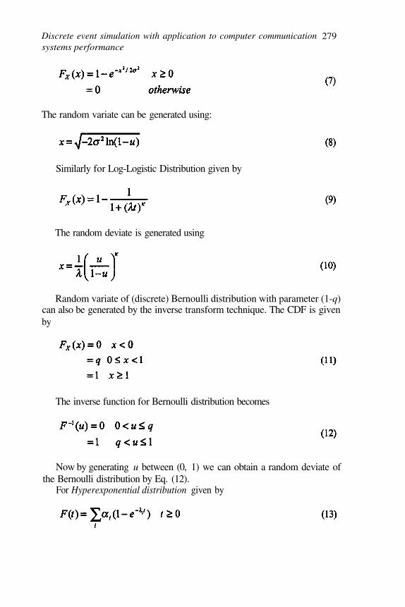
The random variate can be generated using:

Similarly for Log-Logistic Distribution given by

The random deviate is generated using

Random variate of (discrete) Bernoulli distribution with parameter (1-q)can also be generated by the inverse transform technique. The CDF is givenby

The inverse function for Bernoulli distribution becomes

Now by generating u between (0, 1) we can obtain a random deviate ofthe Bernoulli distribution by Eq. (12).

For Hyperexponential distribution given by


Random variate for Hyperexponential can be generated in two steps.Consider for example a three stage Hyperexponential distribution withparameters and First a uniform random number u isgenerated and like Eq. (12) the following inverse function is generated:

Now if and the variate is then generated fromexponential distribution which occur with probability

Similarly if Hyperexponential variate is given as

Similarly depending upon the output of Bernoulli variate,Hyperexponential variate can be generated. Note that this example was fork=3, but it can be easily extended to k=n stages.2. Convolution Method: This is very helpful in such cases when the random

variable Y can be expressed as a sum of other random variables that areindependent and easier to generate than Y. Let

Taking an example of Hypoexponential case, random variable X withparameters is sum of k independent exponential RV’s withmean For example, a 2-stage hypoexponential distribution is given by

From the inverse transform technique, each is generated using Eq. (2)and their sum is the required result. Note that Erlang is a special case of the


281

Hypoexponential distribution when all the k sequential phases have identicaldistribution. Random variate for hypoexponential distribution is given as Eq.(19).

Binomial random variable is known to be the sum of n independent andidentically distributed Bernoulli random variables hence generating nBernoulli random variates and adding, this sum will result in a randomvariate of the Binomial. If are the Bernoulli random variatesgiven by Eq.(12) and let y be Binomial random variate then,

3. Direct Transform of Normal Distribution: Since inverse of a normaldistribution cannot be expressed in closed form we cannot apply inversetransform method. The CDF is given by:

Figure 2. Polar representation


In order to derive a method of generating a random deviate of thisdistribution, we use a property of the normal distribution that relates it tothe Rayleigh distribution. Assume that and are independentstandard normal random variables. Then the square root of their sum

is known to have the Rayleigh distribution [1] for which weknow how to generate its random deviate.

Now in polar coordinates, the original normal random variable can bewritten as:

Using the inverse transform technique (see Eq. 8) we have:

Next we generate a random value of to finally get two randomdeviates of the standard normal:

4.2 Output Analysis

Discrete-event simulation takes random numbers as inputs that result in eachset of study to produce different set of outputs. Output analysis is done toexamine data generated by a simulation. It can be used to predict theperformance/reliability/availability of a system or compare attributes ofdifferent systems. While estimating some measure of the system,

simulation will generate an of due to presence of random

variability. The precision of the estimator will depend upon its variance.Output analysis will help in estimating this variance and also in determiningnumber of observations needed to achieve a desired accuracy. Phenomenon

like sampling error and systematic error influence how well an estimatewill Sampling error is introduced due to random inputs and


283

dependence or correlation among observations. Systematic errors occur dueto dependence of the observations on initially chosen state and initialcondition of the system.

4.2.1 Point and Interval Estimates

Estimation of parameter by a single number from the output of asimulation is called point estimate. Let random variables are setof observations obtained after simulation. Then a common point estimatorfor parameter is given by Eq. (25).

The point estimator is also a random variable and called unbiased ifits expected value is i.e.

If then b is called bias of the point estimator.

The confidence interval provides an interval or range of values aroundthe point estimate [1]. Confidence interval is defined as

For a single parameter, such as the mean, the standard deviation, orprobability level, the most common intervals are two sided (i.e., the statisticis between the lower and upper limit) and one sided (i.e., the statistic issmaller or larger than the end point). For the simultaneous estimation of twoor more parameters, a confidence region, the generalization of a confidenceinterval, can take on arbitrary shapes [24, 25].


4.2.2 Terminating vs. Steady State simulation

Output analysis is discussed here for two classes of simulations:terminating simulation and steady state simulation.

Terminating simulation: This applies to the situation wherein we areinterested in the transient value of some measure, e.g., channel utilizationafter 10 minutes of system operation or the transient availability of thesystem after 10 hours of operation. In these cases each simulation run isconducted until the required simulated time and from each run a singlesample value of the measure is collected. By making m independentsimulation runs, point and interval estimates of the required measure areobtained using standard statistical techniques. In both the cited examples,each simulation run will provide a binary value of the measure and hence weuse the inference procedure based on sampling from the Bernoulli randomvariable [1]. Yet another situation for terminating simulation arises when thesystem being modeled has some absorbing states. For instance we areinterested in estimating the mean time to failure of a system then form eachsimulation run a single value is obtained and multiple independent runs areused to get the required estimate. In this case, we could use inferenceprocedure assuming sampling from the exponential or the Weibulldistribution [1].

Steady-State Simulation: In this case, we can in principle make independentruns but since the transient phase needs to be thrown away and since it canbe long, this approach is wasteful. Attempt is therefore made to get therequired statistics from a long single run. The first problem encountered thenis to estimate the length of the transient phase. The second problem is thedependence in the resulting sequence. [1] talks about how to estimate thecorrelation in the sequence first using independent runs. Instead of usingindependent runs, we can divide a single sequence into first the transientphase and then a batch of steady state runs. Then there are dependencies notonly within a batch but also across batches.

The estimator random variable of the mean measure, to be estimated isgiven by Eq. (28) where n is number of observations.

This value should be independent of the initial conditions. But in realsystem, simulation is stopped after some number of observations n havebeen collected. The simulation run length is decided on the basis of how


285

large the bias in the point estimator is, the precision desired or resourceconstraint for computing.

4.2.3 Initialization Bias

Initial conditions may be artificial or unrealistic. There are methods thatreduce the point-estimator bias in steady state simulation. One method iscalled intelligent initialization that involves initialization of simulation in astate that is more representative of long-run conditions. But if the systemdoesn’t exist or it is very difficult to obtain data directly from the system,any data on similar systems or simplified model is collected.

The second method involves dividing the simulation into two phases.One of them is called the initialization phase from time 0 to and the otheris called the data-collection phase from to

Figure 3. Initialization and Data Collection phase

The choice of is important as system state at time willbe more representative of steady state behavior than at the time of original

five times

4.2.4 Dealing with Dependency [1]

Successive values of variables monitored from a simulation run exhibitdependencies, such as high correlation between the response times ofconsecutive requests to a file server. Assume that the observed quantities aredependent random variables, having index invariant meanand variance The sample mean is given by

initial conditions (i.e., at time t=0). Generally is taken to be more than


Sample mean is unbiased point estimator of population mean butvariance of sample mean is not equal to Taking sequence to be widesense stationary the variance is given by Eq.(30)

The statistic approaches standard normal distribution as m

approaches infinity. Therefore an approximate confidenceinterval becomes

The need to estimate can be avoided using Replication method. It is usedto estimate point-estimator variability. In this method, simulation experimentis replicated m times with n observations each. If initial state is chosenrandomly for all m observations, the result will be independent of each other.But the n observations within each experiment will be dependent. Let thesample mean and sample variance of the experiment be given by

and respectively. From individual sample means, point

estimator of population mean is given by


287

All are independent and identically distributed (i.i.d)

random variables. Assume that the common variance of is denoted byThe estimator of the variance is given by

batches), each having length n. The sample mean of segment is thentreated as an individual observation. This method called the method of batchmeans, reduces the unproductive portion of simulation time to just one initialstabilization period. But the disadvantage is the set of sample means are notstatistically independent and usually the estimator is biased. Estimation ofthe confidence interval for a single run method can be done following thesame procedure as done for replication method. We just replacereplication in independent replication by the batch. Method of batchmeans is also called single run method.

4.2.6 Variance Reduction Techniques

Variance reduction techniques help in obtaining greater precision ofsimulation results (smaller confidence interval) for the same number ofsimulation runs, or in reducing the number of runs required for the desiredprecision. They are used to improve the efficiency and accuracy of thesimulation process.

And confidence interval for is approximately given by

where ‘t’ represents t-student distribution with (m-1) degree of freedom.

4.2.5 Method of Batch Means

One major disadvantage of the replication method is that initialization phasedata from each replication is wasted. To address the issue, we use a designbased on a single, long simulation run divided into contiguous segments (or


One of frequently used technique is importance sampling [12, 13, 14]. Inthis approach the stochastic behavior of the system is modified in such a waythat some events occur more often. This helps in dealing with rare eventsscenarios. But this modification causes model to be biased, which can beremoved using the likelihood ratio function. If carefully done, the varianceof the estimator of the simulated variable is smaller than the originalimplying reduction in the size of the confidence interval. Other techniquesinclude importance splitting [15, 16, 17] and regenerative simulation [18].

Some of the other methods that are used to speed up of simulations areparallel and distributed simulation [10, 11].

To summarize, before generating any sound conclusions on the basis ofthe simulation-generated output data, a proper statistical analysis is required.The simulation experiment helps in estimating different measures of thesystem. The statistical analysis helps in acquiring some assurance that theseestimates are sufficiently precise for the proposed use of the model.Depending on the initial conditions and choice of run length terminatingsimulations or steady-state simulations can be performed. Standard error or aconfidence interval can be used to measure the precision of point estimators.

5. SOME APPLICATIONS

In this section we discuss some of the simulation packages like OPNETMODELER [21] and ns-2 [22]. We also discuss Network Animator (NAM)[30] which generates graphs and animation in ns-2. OPNET MODELER andns-2 are application oriented simulation packages. While OPNETMODELER uses GUI extensively for configuring network, ns-2 is OTclInterpreter and uses code in OTCL and C++ to connect network.

5.1 OPNET MODELER

This simulation package uses an object oriented approach in formulatingthe simulation model. One of the powers of OPNET MODELER comesfrom its simplicity that is due to its menu-driven graphical user interface.Some of the application areas where OPNET can be used are:1.

2.3.

For network (LAN/WAN) planning. It has built-in libraries for all thestandard TCP/IP protocol and applications including IP Quality ofService (QoS), Resource Reservation Protocol (RSVP) etc.It supports wireless and satellite communication schemes and protocols.It can be used for microwave and fiber-optic based network management.


289

4. Can be used for evaluating new routing algorithms for routers, switchesand other connecting devices, before plugging them physically in thenetwork.

Features of OPNET MODELER that make it a comprehensive tool forsimulation are:1.

2.

3.

4.

5.

6.

It uses hierarchical model structure. The model can be nested withinlayers.Multiple scenarios can be simulated simultaneously and results can becompared. This is very useful when deciding the amount of resourceneeded for a network configuration. This also helps in pinpointing whichsystem parameter is affecting the system output most.OPNET MODELER gives an option of importing traffic patterns from anexternal source.It has many of built-in graphing tools that make the output analysiseasier.It has the capability of automatically generating models with live networkinformation (topobgy, device configurations, traffic flows, networkmanagement data repositories, etc.).OPNET MODELER has animation capabilities that can help inunderstanding and debugging the network.

5.1.1 Construction of Model in OPNET MODELER [19]

OPNET MODELER allows to model network topologies using threehierarchical levels:1.

2.

Network Level: It is the highest level of modeling in OPNETMODELER. Topologies are modeled using network level componentslike routers, hosts and links. These network models can be dragged anddropped from object palette, can be chosen from OPNET MODELERmenu which contain numerous topologies like star, bus, ring, mesh etc. orcan be imported from a real network by collecting network topologyinformation. (See Fig. 4)Node level: It is used to model internal structure of a network levelcomponent. It captures the architecture of a network device or system bydepicting the interactions between functional elements called modules.Modules have the capability of generating, sending and receiving packetsfrom other modules to perform their functions within the node. Theytypically represent applications, protocol layers and physical resourcesports, buses and buffers. Modules are connected by “streams” that can bea packet stream, a statistic stream or an association stream. As the namesuggests packet stream represents packet flows between modules, a


3.

statistic stream is used to convey statistics of the between modules. Anassociation stream is used for logically associating different modules andit does not carry any information. (See Fig. 5)Process Level: It uses a Finite State Machine (FSM) description tosupport specification at any level of detail of protocols, resources,applications, algorithms and queuing policies. States and transitionsgraphically define the evolution of a process in response to events. Eachstate of the process model contains C/C++ code, supported by anextensive library for protocol programming. Actions taken in a state aredivided into enter executives and exit executives which are described byProto-C (See Fig. 6).

Figure 4. Screen Shot for Network level Modeling. Detail of an FIFO architecture.


291

Figure 5. Screen Shot for Node level Modeling. Detail of server using Ethernet link.

Figure 6. Screen Shot for Process Level Modeling. Details of an IP Node


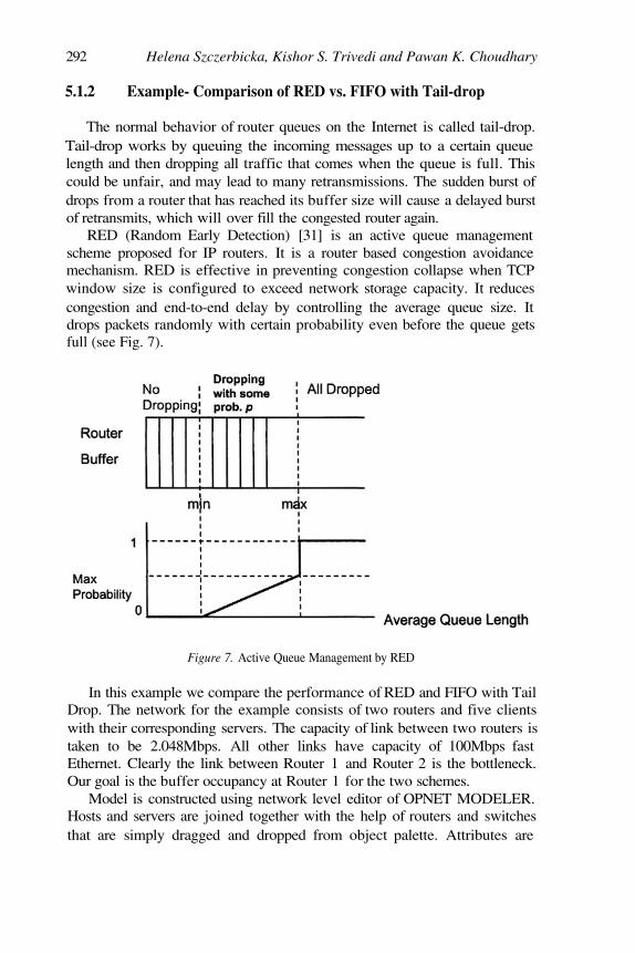
5.1.2 Example- Comparison of RED vs. FIFO with Tail-drop

The normal behavior of router queues on the Internet is called tail-drop.Tail-drop works by queuing the incoming messages up to a certain queuelength and then dropping all traffic that comes when the queue is full. Thiscould be unfair, and may lead to many retransmissions. The sudden burst ofdrops from a router that has reached its buffer size will cause a delayed burstof retransmits, which will over fill the congested router again.

RED (Random Early Detection) [31] is an active queue managementscheme proposed for IP routers. It is a router based congestion avoidancemechanism. RED is effective in preventing congestion collapse when TCPwindow size is configured to exceed network storage capacity. It reducescongestion and end-to-end delay by controlling the average queue size. Itdrops packets randomly with certain probability even before the queue getsfull (see Fig. 7).

Figure 7. Active Queue Management by RED

In this example we compare the performance of RED and FIFO with TailDrop. The network for the example consists of two routers and five clientswith their corresponding servers. The capacity of link between two routers istaken to be 2.048Mbps. All other links have capacity of 100Mbps fastEthernet. Clearly the link between Router 1 and Router 2 is the bottleneck.Our goal is the buffer occupancy at Router 1 for the two schemes.

Model is constructed using network level editor of OPNET MODELER.Hosts and servers are joined together with the help of routers and switchesthat are simply dragged and dropped from object palette. Attributes are


293

assigned for various components. Configuration parameters are assignedwith the help of utility objects. Some of the utility objects like Applicationconfiguration, Profile configuration and QoS configuration are shown infollowing screen shots. The application chosen is video conferencing witheach of the clients having different parameters set- Heavy, StreamingMultimedia, Best Effort, Standard and with Background Traffic. Incomingand outgoing frame sizes are set to 1500 bytes.

All the screen shots from (Fig.8-11) were for the FIFO scheme. OPNETMODELER has a facility for generating duplicate scenario using which wegenerate the model for the RED scheme. The applications and profileconfiguration for RED remains the same as in the FIFO case. Only the QoSattributes configuration needs to be changed (See Fig. 12). RED parametersare set as in Table 1. After this, discrete event simulation is run and differentstatistics like buffer size for Router 1 are collected. All five clients aresending video packets having length 1500 bytes with interarrival time andservice time derived from constant distribution.

Figure 8. Network level modeling for FIFO arrangement. 5 clients are connected to 2switches and 2 routers. They are connected with 5 servers.


Figure 9. Application Configuration- Different window showing assignment of parameter tovideo conferencing (streaming Multimedia)

Figure 10. Profile Configuration -Different Screen shot for entering Video conferencing(various modes) to each of the client.


295

Figure 11 QoS Attribute Configuration- This shows that FIFO is selected with queue size of100 and RED is disabled.

Figure 13 shows the result of simulation where the buffer sizes for thetwo cases are plotted as a function of time. Notice that both buffers usingRED and FIFO taildrop behave similarly when link utilization is low. After40 seconds, when utilization jumps to almost 100 %, congestion starts tobuild at router buffer that uses FIFO taildrop. In case of active queuemanagement (RED case), the buffer occupancy remains low and it neversaturates. In fact buffer occupancy is much smaller than that of FIFO duringthe congestion period.


Figure 12. QoS Attribute configuration for RED case. Application and Profile configurationremains same as FIFO

Figure 13. RED vs. FIFO for buffer occupancy


297

5.2 ns-2 and NAM

Network Simulator (ns) started as a variant of REAL network simulator[32] with the support of DARPA and several companies/universities. It hasevolved and is now known as ns-2. It is a public domain simulation packagein contrast to OPNET MODELER which is a commercial package. LikeOPNET MODELER, it also uses an object oriented approach towardsproblem solving. It is written in C++ and object oriented TCL [33]. Allnetwork components and characteristics are represented by classes. ns-2provides a substantial support for simulation of TCP, routing and multicastprotocols over wired and wireless networks. Details about ns -2can be foundfrom http://www.isi.edu/nsnam/ns/.

5.2.1 Overview and Model construction in ns-2

ns-2 provides canned sub-models for several network protocols like TCPand UDP, router queue management mechanism like Tail Drop, RED,routing algorithms like Dijkstra [34] and traffic source behavior like telnet,FTP, CBR etc. It contains simulation event scheduler and a large number ofnetwork objects, such as routers, links etc. which are interconnected to forma network. The user needs to write an OTc1 script that initiates an eventscheduler, sets up the network topology using network objects and tellstraffic sources when to start and stop transmitting packets through the eventscheduler.

5.2.2 Network Components (ns objects)

Objects are built from a hierarchical C++ class structure. As shown inFig. 14, all objects are derived from class NsObject. It consists of twoclasses- connectors and classifiers. Connector is an NsObject from whichlinks like queue and delay are derived. Classifiers examine packets andforward them to appropriate destinations. Some of the most frequently usedobjects are:1.

2.

Nodes: This represents clients, hosts, router and switches. For example, anode n1 can be created by using command set n1 [$ns node].Classifiers: It determines the outgoing interface object based on sourceaddress and packet destination address. Some of the classifiers areAddress classifier, Multicast classifier, Multipath classifier andReplicators.


Figure 14. Class Hierarchy (Taken from “NS by example” [35])

3.

4.

5.

6.

Links: These are used for connection of nodes to form a networktopology. A link is defined by its head which becomes its entry point, areference to main queue element and a queue to process packets droppedat the link. Its format is $ns <type>-link <nodel> <node2><bandwidth> <delay> <queue-type>.Agents: these are the transport end-points where packets originate or aredestined. Two types of agents are TCP and UDP. ns-2 supports widevariants of TCP and it gives an option for setting ECN bit specification,congestion control mechanism and window settings. For more detailsabout Agent specification see [14]Application: The major types of applications that ns-2 supports are trafficgenerators and simulated applications. Attach-agent is used to attachapplication to transport end-points. Some of the TCP based applicationssupported by ns-2 are Telnet and FTP.Traffic generators: In cases of a distribution driven simulation automatedtraffic generation with desired shape and pattern is required. Some oftraffic generators which ns-2 provide are Poisson, On-OFF, Constant bitrate and Pareto On-OFF.

5.2.3 Event Schedulers

Event scheduler is used by network components that simulate packet-handling delay or components that need timers. The network object thatissues an event will handle that event later at a scheduled time. Eventscheduler is also used to schedule simulated events, such as when to start aTelnet application, when to finish a simulation, etc. ns -2 has real-time and


299

non-real-time event schedulers. Non-real-time scheduler can be implementedeither by a list, heap or a calendar.

5.2.4 Data collection and Execution

ns-2 uses tracing and monitoring for data collection. Events such as apacket arrival, packet departure or a packet drop from a link/queue arerecorded by tracing. Since tracing module does not collect data for anyspecific performance metrics, it is only useful for debugging and verificationpurposes. The command in ns-2 for activating tracing is $ns trace-all<tracefile>.

Monitoring is a better alternative to tracing where we need to monitor aspecific link or node. Several trace objects are created which are theninserted into a network topology at desired places. These trace objectscollect different performance metrics. Monitoring objects can also be writtenin C++ (Tracing can written in OTcl only) and inserted into source or sinkfunctions.

After constructing network model and setting different parameters, ns-2model is executed by using run command. ($ns run).

5.2.5 Network Animator

NAM is an animation tool that is used extensively along with ns -2. It wasdeveloped in LBL. It is used for viewing network simulation packet tracesand real world packet traces. It supports packet level animation that showspackets flowing through the link, packets being accumulated in the bufferand packets dropping when the buffer is full. It also supports topology layoutthat can be rearranged to suit user’s needs. It has various data inspectiontools that help in better understanding of the output. More information aboutNAM can be found at http://www.isi.edu/nsnam/ns/tutorial/index.html.

5.2.6 Example- RED Analysis

Objective: Studying the dynamics of current and average queue size in aRED queue.

In this example we have taken six nodes. All links are duplex in naturewith their speed and delay shown in the Fig.16. In this example FTPapplication is chosen for both source nodes n1 and n3. Node n2 is the sinknode. The window size for TCP application is taken to be 15. RED buffercan hold a maximum of 30 packets in this example. First FTP applicationstarts from 0 till 12 seconds and second FTP application starts from 4 to 12


seconds. For output data collection, monitoring feature is used. NAM is usedto display graph of buffer size vs. time

Figure 15. NAM Window (picture taken from “Marc Greis Tutorial” [36])

In this File Transfer Protocol has been simulated over TCP network. Bydefault FTP is modeled by simulating the transfer of a large file between twoendpoints. By large file we mean that FTP keeps on packetizing the file andsending it continuously between the specified start and stop times. Thenumber of packets to be sent between start and stop time can also bespecified using produce command. Traffic is controlled by TCP whichperforms the appropriate congestion control and transmits the data reliably.The buffer size is taken to be 14000 packets and router parameters are givenin table 2. The output shows the buffer occupancy at router r1, forinstantaneous and average value case. From the graph it becomes clear thatduring higher utilization also, RED helps in reducing congestion.


301

Figure 16. Network connection for an RED configuration

6. SUMMARY

This tutorial discussed simulation modeling basics and some of itsapplications. Role of statistics in different aspects of simulation wasdiscussed. This includes random variate generation and the statisticalanalysis of simulation output.

Different classes of simulation were discussed. Simulation packages likeOPNET MODELER and ns-2 along with some applications were discussedin the last section. These packages are extensively used in research andindustry for real-life applications.

Helena Szczerbicka, Kishor S. Trivedi and Pawan K. Choudhary

Figure 17. Plot of RED Queue Trace path

REFERENCES

1.

2.

3.

4.

5.6.7.8.

Kishor S. Trivedi, Probability and Statistics with Reliability, Queuing,and Computer Science Applications, (John Wiley and Sons, New York,2001).Robin A. Sahner, Kishor S. Trivedi, and Antonio Puliafito, Performanceand Reliability Analysis of Computer Systems: An Example-BasedApproach Using the SHARPE Software Package, (Kluwer AcademicPublishers, 1996).Kishor S. Trivedi, G. Ciardo, and J. Muppala, SPNP: Stochastic Petri NetPackage, Proc. Third Int. Workshop on Petri Nets and PerformanceModels (PNPM89), Kyoto, pp. 142 - 151, 1989.J. Banks, John S. Carson, Barry L. Nelson and David M. Nicol, Discrete–Event System Simulation, Third Edition, (Prentice Hall, NJ, 2001).Simula Simulator; http://www.isima.fr/asu/ .Simscript II.5 Simulator; http://www.caciasl.com/ .AUTOMOD Simulator; http://www.autosim.com/.CSIM 19 Simulator; http://www.mesquite.com/.

302


303

9.

10.

11.

12.

13.

14.

15.

16.

17.

18.

19.

20.

21.22.23.

K, Pawlikowski, H. D. Jeong and J. S. Lee, On credibility of simulationstudies of telecommunication networks, IEEE Communication Magazine,4(1), 132-139, Jan 2002.H. M. Soliman, A.S. Elmaghraby, M.A. El-sharkawy, Parallel andDistributed Simulation System: an overview, Proceedings of IEEESymposium on Computer and Communications, pp 270-276, 1995.R.M. Fujimoto, Parallel and Distributed Simulation System, Simulation

Conference, Proceeding of winter, Vol. 1, 9-12 Dec. 2001.B. Tuffin, Kishor S. Trivedi, Importance Sampling for the Simulation ofStochastic Petri Nets and Fluid Stochastic Petri Nets, Proceeding of HighPerformance Computing, Seattle, WA, April 2001.G. S. Fishman, Concepts Algorithms and Applications, (Springer-Verlag,1997).P.W. Glynn and D.L. Iglehart, Importance Sampling for stochasticSimulations, Management Science, 35(11), 1367-1392, 1989.P. Glasserman, P. Heidelberger, P. Shahabuddin, and T. Zajic, Splitting

for rare event simulation: analysis of simple cases. In Proceedings of the1996 Winter Simulation Conference edited by D.T. Brunner J.M.Charnes, D.J. Morice and J.J. Swain editors, pages 302-308, 1996.P. Glasserman, P. Heidelberger, P. Shahabuddin, and T. Zajic, A look at

multilevel splitting. In Second International conference on Monte-Carloand Quasi- Monte Carlo Methods in Scientific Computing edited by G.Larcher, H. Niederreiter, P. Hellekalek and P. Zinterhof, Volume 127 ofLecture Series in Statistics, pages 98-108, (Springer-Verlag, 1997).B. Tuffin, Kishor S. Trivedi, Implementation of Importance Splitting

techniques in Stochastic Petri Net Package,” in Computer performanceevaluation: Modeling tools and techniques; 11th InternationalConference; TOOLS 2000, Schaumburg, Il. USA, edited by B. Haverkort,H. Bohnenkamp, C. Smith, Lecture Notes in Computer Science 1786,(Springer Verlag, 2000).S. Nananukul, Wei-Bo-Gong, A quasi Monte-Carlo Simulation forregenerative simulation, Proceeding of 34th IEEE conference onDecision and control, Volume 2, Dec. 1995.M. Hassan, and R. Jain, High Performance TCP/IP Networking:Concepts, Issues, and Solutions, (Prentice-Hall, 2003).Bernard Zeigler, T. G. Kim, and Herbert Praehofer, Theory of Modeling

and Simulation, Second Edition, (Academic Press, New York, 2000).OPNET Technologies Inc.; http://www.opnet.com/.Network Simulator; http://www.isi.edu/nsnam/ns/.Arena Simulator; http://www.arenasimulation.com/.


24.

25.

26.

27.

28.

29.

30.31.

32.

33.

34.

35.36.

Liang Yin, Marcel A. J. Smith, and K.S. Trivedi, Uncertainty analysis inreliability modeling, In Proc. of the Annual Reliability andMaintainability Symposium, (RAMS), Philadelphia, PA, January 2001.Wayne Nelson. Applied Life Data Analysis John Wiley and Sons, NewYork, 1982.L.W. Schruben, Control of initialization Bias in multivariate simulationresponse, Communications of the Association for Computing machinery,246-252, 1981.A.M. Law and J.M. Carlson, A sequential Procedure for determining thelength of steady state simulation, Operations Research, Vol. 27, pp-131-143, 1979.Peter P. Welch, Statistical analysis of simulation result, Computerperformance Modeling Handbook, edited by Stephen S. Lavenberg,Academic Press, 1983W.D. Kelton, Replication Splitting and Variance for simulating DiscreteParameter Stochastic Process, Operations Research Letters, Vol.4,pp-275-279, 1986.Network Animator.; http://www.isi.edu/nsnam/nam/.S. Floyd, and V. Jacobson, Random early detection gateways forcongestion avoidance, IEEE/ACM Transactions on Networking,Volume1, Issue 4 , Aug. 1993 Pages:397– 413.REAL network simulator.;

http://www.cs.cornell.edu/skeshav/real/overview.htmlOTCL-Object TCL extensions.;http://bmrc.berkeley.edu/research/cmt/cmtdoc/otcl/E. W. Dijkstra, A Note on Two Problems in Connection with Graphs.

Numerische Math. 1, 269-271, 1959.Jay Cheung, Claypool, NS by example.; http://nile.wpi.edu/NS/Marc Greis, Tutorial on ns.; http://www.isi.edu/nsnam/ns/tutorial/

discrete event simulation with ... - home - springer · discrete event simulation with application...

Documents