using a decoupling technique to identify the magnetic … · using a decoupling technique to...

Using a Decoupling Technique to Identify theMagnetic Flux in a Permanent Magnet Synchronous

MotorPaolo Mercorelli

Abstract—Unknown parameters cause difficulties in the con-trol of permanent magnetic motors. Particular techniques arerequested to be able to achieve an appropriately controlleddynamics identification. A geometric approach for achieving adecoupling of the system is applied in the presented strategy.The decoupling makes the estimation of the Permanent MagnetSynchronous Motor (PMSM) parameters easier. A feedbackcontroller in combination with the feed-forward controller beinggenerated by an input partition, achieves the decoupling. Thiscan be applied to various types of motors or systems in caseof the decoupling conditions being satisfied. A control togetherwith the identification method is tested in the simulation section.The presented simulation and measured results are shown forvalidation of the strategy which is proposed.

Index Terms—Permanent Magnet Synchronous Motor, Identi-fication, PWM control

I. INTRODUCTION AND MOTIVATIONS

REcently the interest in the topic of geometric control hasincreased in theoretical aspects and applications as well,

see for instance [1], particulary in control problems like Non-interaction and Model Predictive Control, see [2]. It is knownthat, an accurate knowledge of the model and its parametersis necessary for realising an effective control. For achievinga desired system performance, advanced control systems areusually required to provide fast and accurate response, quickdisturbance recovery and parameter variations insensitivity [3].Acquiring accurate models for systems under investigationis usually the fundamental part in advanced control systemdesigns, see [4]. In [4] a Permanent Magnet SynchronousMotor (PMSM) is considered with a PI controller. A chopperstrategy is proposed and a parameter set up of the abovementioned PI-regulator is proposed to obtain a smooth trackingdynamics even though a chopper control structure is includedin the drive. High performance application of permanentmagnet synchronous motors (PMSM) is increasing. In par-ticular, application in electrical vehicles is very much used.The existing applications chopper control structures are verypopular because they are very cheep and easy to be realised.Nevertheless, using a chopper control structure smooth track-ing dynamics could be difficult to obtain without increasing theswitching frequency because of the discontinuity of the controlsignals. No smooth tracking dynamics lead to a not comfort-able travel effect for the passengers of the electrical vehicle.

Paolo Mercorelli is with the Institute of Product and Process Innova-tion, Leuphana University of Lueneburg, Volgershall 1, D-21339 Lueneb-urg, Germany Tel.: +49-(0)4131-677-5571, Fax: +49-(0)[email protected].

PMSMs as traction motors are common in electric or hybridroad vehicles and they importance will increase in the futurebecause of the dissemination of electrical mobility. Moreover,in electrical mobility the control strategies, connected with anoptimal energy management, represent a decisive point for thesuccess of effective technologies and products, [5]. PMSMshave, in term of control, already consolidated methods andtechniques. For rail vehicles, PMSMs as traction motors arenot widely used yet. Although the traction PMSM can bringmany advantages, just a few prototypes of vehicles were builtand tested. The next two new prototypes of rail vehicles withtraction PMSMs were presented on InnoTrans fair in Berlin2008 Alstom AGV high speed train and skoda Transportationlow floor tram 15T ForCity. Advantages of PMSM are wellknown. The greatest advantage is low volume of the PMSM incomparison with other types of motors. It makes a direct driveof wheels possible. On the other hand, the traction drive withPMSM has to meet special requirements typical for overheadline fed vehicles.

The most common parameters required for theimplementation of such advanced control algorithms arethe classical simplified model parameters: Ld - the directaxis self-inductance, Lq - the quadrature axis self-inductance,and Φ - the permanent magnet flux linkage. Techniqueshave been proposed for the parameters’ identification of aPMSM from different perspectives, such as offline [6], [7]and online identification of PMSM electrical parameters,[8]. These techniques are based on the decoupled controlof linear systems when the motor’s mechanical dynamicsare ignored. Using a decoupling control strategy, internaldynamics may be almost obscured, but it is useful toremember that there are no limitations in the controllabilityand observability of the system. In the report by [9] adecoupling technique is used to control a permanent magnetsmachine more efficiently in a sensorless way using anobserver. Despite limitations on the frequency range ofidentification, this paper proposes a dynamic observer basedon a geometric decoupling technique to estimate parameterΦ. The proposed identification technique, similar to thatpresented in [10], applies a procedure based on the workin [11]. In the meantime, the paper proposes a particularobserver that identifies the permanent magnet flux usingthe estimated Ldq and Rs parameters from an ARMAidentification structure as presented in [11]. The paper isorganised in the following way: a sketch of the modelof the synchronous motor and its behaviour are given in

INTERNATIONAL JOURNAL OF CIRCUITS, SYSTEMS AND SIGNAL PROCESSING Volume 9, 2015

ISSN: 1998-4464 1

Section II, Section III is devoted to deriving, proposing anddiscussing the dynamic estimator, and Section IV showsthe simulation results using real data for a three-phase PMSM.

The main nomenclatureuin(t) = [ua(t), ub(t), u0(t)]

T : three phase inputvoltage vectori(t) = [ia(t), ib(t), i0(t)]

T : three phase inputcurrent vectoruq(t): induced voltage vectorωel: electrical pulsationRs: coil resistanceLdq: dq coil inductanceA: state matrix of the electrical modelB: input matrix of the electrical modelB = imB: image of matrix B (subspace spannedby the columns of matrix B)minI(A,B) =

∑n−1i=0 AiimB: minimum A–

invariant subspace containing im(B)F: decoupling feedback matrix fieldg(ωel): Park transformationT(ωel): decoupling feedforward matrix fieldI: invariant subspaceCd: kernel of output matrix Cd (d component ofthe current)Cq: kernel of output matrix Cq (q component ofthe current)C0: kernel of output matrix C0 (0 component ofthe current)

II. MODEL OF A SYNCHRONOUS MOTOR

For aiding advanced controller design for PMSM, it is veryimportant to obtain an appropriate model of the motor. Agood model should not only be an accurate representation ofsystem dynamics but it should also facilitate the applicationof the existing control techniques. Among a variety of modelspresented in the literature since the introduction of PMSM,the two-axis dq-model, obtained using Park dq-transformationis the most widely used in variable speed PMSM drivecontrol applications [3] and [8]. The Park dq-transformationis a coordinate transformation that converts the three-phasestationary variables into variables in a rotating coordinatesystem. In dq-transformation, the rotating coordinate is definedrelative to a stationary reference angle as illustrated in Fig. 1.The dq-model is considered in this work.[

ud(t)uq(t)u0(t)

]=[

2 sin(ωelt)3

2 sin(ωel−2π/3)3

2 sin(ωel+2π/3)3

2 cos(ωelt)3

2 cos(ωel−2π/3)3

2 cos(ωel+2π/3)3

13

13

13

] [ua(t)ub(t)uc(t)

], (1)

[id(t)iq(t)i0(t)

]=[

2 cos(ωelt)3


2 cos(ωel+2π/3)3

−2 sin(ωelt)3

−2 sin(ωel−2π/3)3

−2 sin(ωel+2π/3)3

13

13

13

] [ia(t)ib(t)ic(t)

].

(2)

Fig. 1. Park transformation for the motor

The dynamic model of the synchronous motor in dq-coordinates can be represented as follows:[

did(t)dt

diq(t)dt

]=

[−Rs

Ld

Lq

Ldωel(t)

−Rs

Lq−Ld

Lqωel(t)

][id(t)iq(t)

]+[

1Ld

0

0 1Lq

][ud(t)uq(t)

]−

[0

Φωel(t)Lq

], (3)

andMm =

3

2p{Φiq(t) + (Ld − Lq)id(t)iq(t)}. (4)

In (3) and (4), id(t), iq(t), ud(t) and uq(t) are the dq-components of the stator currents and voltages in syn-chronously rotating rotor reference frame, ωel(t) is the rotorelectrical angular speed, the parameters Rs, Ld, Lq , Φ andp are the stator resistance, d-axis and q-axis inductance, theamplitude of the permanent magnet flux linkage, and p thenumber of couples of permanent magnets, respectively. At theend, Mm indicates the motor torque. Considering an isotropicmotor with Ld ≃ Lq = Ldq , it follows:[

did(t)dt

diq(t)dt

]=

[− Rs

Ldqωel(t)

− Rs

Ldqωel(t)

] [id(t)iq(t)

]+

[1

Ldq0

0 1Ldq

][ud(t)uq(t)

]−

[0

Φωel(t)Ldq

], (5)

andMm =

3

2pΦiq(t), (6)

with the following movement equation:

Mm −Mw = Jdωmec(t)

dt, (7)

where pωmech(t) = ωel(t) and Mw is an unknown mechanicalload.


ISSN: 1998-4464 2

III. DESIGN OF A DECOUPLING CONTROL STRATEGY

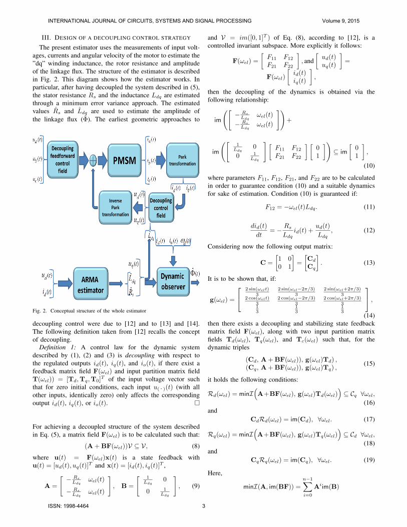
The present estimator uses the measurements of input volt-ages, currents and angular velocity of the motor to estimate the”dq” winding inductance, the rotor resistance and amplitudeof the linkage flux. The structure of the estimator is describedin Fig. 2. This diagram shows how the estimator works. Inparticular, after having decoupled the system described in (5),the stator resistance Rs and the inductance Ldq are estimatedthrough a minimum error variance approach. The estimatedvalues Rs and Ldq are used to estimate the amplitude ofthe linkage flux (Φ). The earliest geometric approaches to

Fig. 2. Conceptual structure of the whole estimator

decoupling control were due to [12] and to [13] and [14].The following definition taken from [12] recalls the conceptof decoupling.

Definition 1: A control law for the dynamic systemdescribed by (1), (2) and (3) is decoupling with respect tothe regulated outputs id(t), iq(t), and io(t), if there exist afeedback matrix field F(ωel) and input partition matrix fieldT(ωel)) = [Td,Tq,T0]

T of the input voltage vector suchthat for zero initial conditions, each input u( · )(t) (with allother inputs, identically zero) only affects the correspondingoutput id(t), iq(t), or io(t). �

For achieving a decoupled structure of the system describedin Eq. (5), a matrix field F(ωel) is to be calculated such that:

(A+BF(ωel))V ⊆ V, (8)

where u(t) = F(ωel)x(t) is a state feedback withu(t) = [ud(t), uq(t)]

T and x(t) = [id(t), iq(t)]T ,

A =

[− Rs

Ldqωel(t)

− Rs

Ldqωel(t)

], B =

[ 1Ldq

0

0 1Ldq

], (9)

and V = im([0, 1]T ) of Eq. (8), according to [12], is acontrolled invariant subspace. More explicitly it follows:

F(ωel) =

[F11 F12

F21 F22

], and

[ud(t)uq(t)

]=

F(ωel)

[id(t)iq(t)

],

then the decoupling of the dynamics is obtained via thefollowing relationship:

im

([− Rs

Ldqωel(t)

− Rs

Ldqωel(t)

])+

im

([1

Ldq0

0 1Ldq

][F11 F12

F21 F22

] [01

])⊆ im

[01

],

(10)

where parameters F11, F12, F21, and F22 are to be calculatedin order to guarantee condition (10) and a suitable dynamicsfor sake of estimation. Condition (10) is guaranteed if:

F12 = −ωel(t)Ldq. (11)

did(t)

dt= − Rs

Ldqid(t) +

ud(t)

Ldq, (12)

Considering now the following output matrix:

C =

[1 00 1

]=

[Cd

Cq

]. (13)

It is to be shown that, if:

g(ωel) =

2 sin(ωelt)3

2 sin(ωel−2π/3)3

2 sin(ωel+2π/3)3

2 cos(ωelt)3


2 cos(ωel+2π/3)3

13

13

13

,

(14)then there exists a decoupling and stabilizing state feedbackmatrix field F(ωel), along with two input partition matrixfields Td(ωel), Tq(ωel), and Tc(ωel) such that, for thedynamic triples

(Cd, A+BF(ωel)), g(ωel)Td) ,(Cq, A+BF(ωel)), g(ωel)Tq) ,

(15)

it holds the following conditions:

Rd(ωel) = minI(A+BF(ωel), g(ωel)Td(ωel)

)⊆ Cq ∀ωel,

(16)and

CdRd(ωel) = im(Cd), ∀ωel. (17)

Rq(ωel) = minI(A+BF(ωel), g(ωel)Tq(ωel)

)⊆ Cd ∀ωel,

(18)and

CqRq(ωel) = im(Cq), ∀ωel. (19)

Here,

minI(A, im(BF)) =n−1∑i=0

Aiim(B)


ISSN: 1998-4464 3

is a minimum A–invariant subspace containing im(B). More-over, the partition matrix fields Td(ωel), Tq(ωel) and T0(ωel)satisfy the following relationships:

im(g(ωel) ·Td(ωel)) = im(g(ωel)) ∩Rd(ωel),im(g(ωel) ·Tq(ωel)) = im(g(ωel)) ∩Rq(ωel).

(20)

The stabilizing matrix field F(ωel) is such that:

(A+BF(ωel))Rd(ωel) ⊆ Rd(ωel), (21)

and(A+BF(ωel))Rq(ωel) ⊆ Rq(ωel). (22)

Considering

T(ωel) = [Td(ωel),Tq(ωel),T0(ωel),Tc(ωel)],

where Tc(ωel) is defined in a complementary fashion and it isstraightforward to show that matrix field Tc = 0. In particular,matrix field Tc represents the complementary matrix fieldpartition to the subspaces of d-coordinate, q-coordinate and 0-coordinate. The system is described using just three variables,therefore partition fields Td(ωel) and Tq(ωel) complete thetransformation and thus Tc = 0.

imT(ωel) = im[Td(ωel),Tq(ωel),T0(ωel)] =

imTd(ωel)⊕ imTq(ωel)⊕ imT0(ωel). (23)

Considering the output matrix (13) corresponding to d-coordinate, q-coordinate and 0-coordinate, their respectivekernels are as follows:

Cd = im

[0 01 0

], Cq = im

[1 00 0

]. (24)

According to definition B of Eqs. (9) it is straightforward toobserve that the following three equations hold ∀ ωel:

im(B) ∩ Cq = 0, (25)

im(B) ∩ Cd = 0. (26)

The following calculations allow to get the required fields forthe decoupling of the system:

Td(ωel) = (g(ωel))† · im(B) ∩ Cq, (27)

Tq(ωel) = (g(ωel))† · im(B) ∩ Cd. (28)

Field g(ωel) is a function of ωel without singularities ifωel(t) = kπ with k ∈ N, where with (g(ωel))

† the pseudoinverse of field g(ωel) is indicated. Adding all 3 T-Fieldstogether, we get a new field T(ωel):

T(ωel) = Td(ωel) +Tq(ωel). (29)

Field T(ωel) can be seen as a preselecting field and thefollowing product realises the mechanical decoupling:

B = im(g(ωel)T(ωel)) = im

[1 00 1

], (30)

in which matrix B can be seen as a resulting input matrix.

A. A dynamic estimator of Φ

As it is shown in Fig. 2, parameters Rs and Ldq can beestimated by using an ARMA identification structure. Thesetwo values are needed to estimate flux Φ. If the electrical partof the system ”q” and ”d” axes is considered, then, assumingthat ωel(t) = 0, iq(t) = 0, and id(t) = 0, the followingequation can be considered:

Φ(t) = −Ldq

diq(t)dt +Rsid(t) + Ldqωel(t)iq(t)− uq(t)

ωel(t). (31)

Consider the following dynamic system:

dΦ(t)

dt= −KΦ(t)−

K( Ldq

diq(t)dt + Rsid(t)

ωel(t)+

Ldqωel(t)iq(t) + uq(t)

ωel(t)

), (32)

where K is a function to be calculated. Eq. (32) represents theestimators of Φ and Ldq and Rs represent the estimated in-ductance and resistance respectively by an ARMA proceduresin [11]. If the error functions are defined as the differencesbetween the true and the observed values, then:

eΦ(t) = Φ(t)− Φ(t), (33)

anddeΦ(t)

dt=

dΦ(t)

dt− dΦ(t)

dt. (34)

If the following assumption is given:

∥dΦ(t)dt

∥ << ∥dΦ(t)dt

∥, (35)

then in Eq. (34), the term dΦ(t)dt is negligible. Using Eq. (32),

Eq. (34) becomes

deΦ(t)

dt= KΦ(t)+

K( Ldq

diq(t)dt + Rsid(t)

ωel(t)+


ωel(t)

). (36)

Because of Eq. (31), (36) being able to be written as follows:

deΦ(t)

dt= KΦ(t)−KΦ(t),

and considering (33), then:

deΦ(t)

dt+KΦ(t) = 0. (37)

K can be chosen to make Eq. (37) exponentially stable. Toguarantee exponential stability, K must be

K > 0.

To guarantee ∥dΦ(t)dt ∥ << ∥dΦ(t)

dt ∥, then K >> 0. Theobserver defined in (32) suffers from the presence of thederivative of the measured current. In fact, if measurementnoise is present in the measured current, then undesirablespikes are generated by the differentiation. The proposedalgorithm must cancel the contribution from the measuredcurrent derivative. This is possible by correcting the observed


ISSN: 1998-4464 4

velocity with a function of the measured current, using asupplementary variable defined as:

η(t) = Φ(t) +N (iq(t)), (38)

where N (iq(t)) is the function to be designed.Consider

dη(t)

dt=

dΦ(t)

dt+

dN (iq(t))

dt(39)

and let

dN (iq(t))

dt=

dN (iq)

diq(t)

diq(t)

dt=

KLdq

ωel(t)

diq(t)

dt. (40)

The purpose of (40) is to cancel the differential contributionfrom (32). In fact, (38) and (39) yield, respectively:

Φ(t) = η(t)−N (iq(t)), and (41)

dΦ(t)

dt=

dη(t)

dt− dN (iq(t))

dt. (42)

Substituting (40) in (42) results in:

dΦ(t)

dt=

dη(t)

dt− KLdq

ωel(t)

diq(t)

dt. (43)

Inserting Eq. (43) into Eq. (32), the following expression isobtained:

dη(t)

dt− KLdq

ωel(t)

diq(t)

dt= −KΦ(t)−

K( Ldq

diq(t)dt + Rsid(t)

ωel(t)+


ωel(t)

), (44)

then:

dη(t)

dt= −KΦ(t)−K

(Rsid(t) + Ldqωel(t)iq(t) + uq(t)

)ωel(t)

.

(45)Letting N (iq(t)) = kappiq(t), where a parameter has beenindicated with kapp, then from (40) ⇒ K =

kappωel(t)

Ldq, and

Eq. (41) becomes:

Φ(t) = η(t)− kappiq(t). (46)

Finally, substituting (46) in (45) results in the followingequation:

dη(t)

dt= −kappωel(t)

Ldq

(η(t)− kappiq(t)

)+

kapp

Ldq

(Rsid(t) + Ldqωel(t)iq(t) + uq(t)

),

Φ(t) = η(t)− kappiq(t). (47)

Using the implicit Euler method, the following velocity ob-server structure is obtained:

η(k) =η(k − 1)

1 + tskappωel(k)

Ldq

+

tsk2appωel(k)iq(k)

Ldq+ kappωel(k)iq(k) +

tsRskappid(k)

Ldq

1 + tskappωel(k)

Ldq

iq(k)+

tskapp

Ldq

1 + tskappωel(k)

Ldq

uq(k),

Φ(k) = η(k)− kappiq(k), (48)

where ts is the sampling period.

Remark 1: Assumption (35) states that the dynamics of theapproximating observer should be faster than the dynamics ofthe physical system. This assumption is typical for the designof observers. �

Remark 2: The estimator of Eq. (48) presents thefollowing limitations: for low velocity of the motor(ωmec.(t) << ωmecn(t)), where ωmecn(t) represents thenominal velocity of the motor), the estimation of Φ becomesinaccurate. Because of ωel(t) dividing the state variableη, the observer described by (48) becomes hyperdynamic.Critical phases of the estimation are the starting and endingof the movement. Another critical phase is represented bya high velocity regime. In fact, it has been proven throughsimulations, that if ωmec(t) >> ωmecn(t), then the observerdescribed by (48) becomes hypodynamic. According to thesimulation results, within some range of frequency, thishypo-dynamicity can be compensated by a suitable choice ofkapp. �

Remark 3: The Implicit Euler method guarantees thefinite time convergence of the observer for any choice ofkapp. Nevertheless, any other method can demonstrate thevalidity of the presented results. Implicit Euler method is astraightforward one. �

IV. SIMULATION AND MEASURED RESULTS

The results have been achieved using a special stand with a58-kW traction PMSM. The stand consists of a PMSM, a tramwheel and a continuous rail. The PMSM is a prototype for lowfloor trams. The PMSM parameters are: nominal power of 58kW, nominal torque of 852 Nm, nominal speed of 650 rpm,nominal phase current of 122 A, nominal input voltage of 230V and the number of poles is 44. The model parameters are:R = 0.08723 Ohm, Ldq = Ld = Lq = 0.8 mH, Φ = 0.167Wb. The engine has a nominal power of 55 kW, a nominalvoltage of 380 V and nominal speed of 589 rpm. Figure 4shows the estimation measured results of Φ magnet flux. Fromthese figures, the effect of the limit of the procedure discussedin remark 2 is visible at the beginning of the estimation. Inparticular, this effect is visible in the real measured results.Figure 6 shows a detail of the estimation of the measured


ISSN: 1998-4464 5

0 0.5 1 1.5 2

x 10−3

0

2

4

6

8

10

Time (sec.)

Pe

rma

ne

nt

ma

gn

et

flu

x lin

ka

ge

(V

s)

Estimated values of the permanent magnet flux linkage Real value of the permanent magnet flux linkage

Fig. 3. Simulated results: Estimated and real values of the permanent magnetflux linkage for kapp = 20

0 0.5 1 1.5 2

x 10−3

−20

−15

−10

−5

0

5

10

Time (sec.)

Pe

rma

ne

nt

ma

gn

et

flu

x lin

ka

ge

(V

s)

Estimated values of the flux linkageReal value of the flux linkage

Fig. 4. Measured results

magnetic flux of the motor. In order to recall this effect, it isuseful to say that the critical phases of the estimation are thestarting and ending of the movement. Another critical phaseis represented by a high velocity regime. In fact, it has beenproven through simulations and measured results, so that ifωmec(t) >> ωmecn(t), then the observer described by (48)becomes hypodynamic. Figure 5 shows the angular velocityof the motor. In the present simulations, t = 0 corresponds toωel(t) = 0.

Using a control structure of [15] with PWM frequencyequals 100kHz the same results as in [15] are obtained. Figure

0 0.5 1 1.5 2

x 10−3

−2

0

2

4

6

8

10

Time (sec.)

Pe

rma

ne

nt m

ag

ne

t flu

x lin

ka

ge

(V

s)

Estimated values of the flux linkage Real value of the flux linkage

Fig. 5. Detail of the estimation of the measured magnetic flux

0 0.002 0.004 0.006 0.008 0.01 0.012 0.014 0.016−200

−100

0

100

200

300

400

500

600

700

Time (sec.)

An

gu

lar

ve

locity (

rad

./se

c.)

Fig. 6. Angular velocity

7 shows the obtained and desired motor velocity profiles.Figure 8 shows the obtained and desired motor accelerationprofiles. From these two results it is possible to remark that theeffect of the chopper control is visible which does not allow thetracking to be precise. Figure 9 shows PWM signal sequencewith the maximal chopper switching frequency equals 2.5kHz.Fig. 10 shows the chopper effect on the input of the motor.

V. CONCLUSIONS AND FUTURE WORK

This paper considers a decoupling dynamic estimator forfully automated parameters identification for three-phase syn-chronous motors. The proposed strategy uses the geometric


ISSN: 1998-4464 6

0 0.002 0.004 0.006 0.008 0.01 0.012 0.014 0.016 0.018 0.020.4

0.6

0.8

1.0

1.2

1.4

1.6

1.8

2.0

2.2

Time (sec.)

103 ro

unds

/min

.

Motor velocity

Obtained velocityDesired velocity

Fig. 7. Profile of the obtained and desired motor velocity using a maximalswitching chopper frequency equals 2.5kHz

0 2 4 6 8 10 12 14 16 18

x 10−3

−6

−4

−2

0

2

4

6

x 105

Time (sec.)

roun

ds/m

in2 .

Motor acceleration

Obtained accelerationDesired acceleration

Fig. 8. Profile of the obtained and desired motor acceleration using a maximalswitching chopper frequency equals 2.5kHz

0 0.002 0.004 0.006 0.008 0.01 0.012 0.014 0.016 0.018 0.020

0.5

1

1.5

Time (sec.)

Vol

tage

PWM control signal

Fig. 9. PWM signal used as a chopper with a maximal switching frequencyequals 2.5kHz

0 0.002 0.004 0.006 0.008 0.01 0.012 0.014 0.016 0.018 0.02−300

−200

−100

0

100

200

300

400

Time (sec.)

Vol

tage

Three−phase control signals using PWM as a chopper

Phase onePhase twoPhase three

Fig. 10. Three-phase control signals after the chopper controller using a PWMsingnal with a maximal switching frequency equals 2.5kHz


ISSN: 1998-4464 7

approach to realised a decoupling of the system. The esti-mation of the parameters of the motor is simplified througha decoupling. The decoupling is realised using a feedbackcontroller combined with a feedforward one. The feedforwardcontroller is conceived through an input partition matrix.The proposed dynamic estimator is shown to identify theamplitude of the linkage flux using the estimated inductanceand resistance. Through simulations and measured results ona synchronous motor used in automotive applications, thispaper verifies the effectiveness of the proposed method inidentification of PMSM model parameters and discusses thelimits of the proposed procedure. Simulation and measuredresults are reported to validate the proposed strategy. Futurework includes the estimation of a mechanical load and thegeneral test of the present algorithm using a real motor.

REFERENCES

[1] P. Mercorelli. Invariant subspace for grasping internal forces and non-interacting force-motion control in robotic manipulation. Kybernetika,48(6):12291249, 2012.

[2] P. Mercorelli. Geometric structures using model predictive control foran electromagnetic actuator. WSEAS TRANSACTIONS on SYSTEMS andCONTROL, 9:140–149, 2014.

[3] M.A. Rahman, D.M. Vilathgamuwa, M.N. Uddin, and T. King-Jet.Nonlinear control of interior permanent magnet synchronous motor.IEEE Transactions on Industry Applications, 39(2):408–416, 2003.

[4] P. Mercorelli. A lyapunov approach for a PI-controller with anti-windupin a permanent magnet synchronous motor using chopper control.INTERNATIONAL JOURNAL OF MATHEMATICAL MODELS ANDMETHODS IN APPLIED SCIENCES, 8(1):44–51, 2014.

[5] S. Schmidt and P. Mercorelli. Generating energy optimal powertrainforce trajectories with dynamic constraints.In Proceedings of International Conference on Optimization Techniquesin Engineering (OTENG’13, WSEAS Conference), pages 228–233, An-talya, Turkey, 2013.

[6] A. Kilthau and J. Pacas. Appropriate models for the controls of thesynchronous reluctance machine. In Proceedings of the IEEE IAS AnnualMeeting, pages 2289–2295, Pittsburgh, USA, 2002.

[7] S. Weisgerber, A. Proca, and A. Keyhani. Estimation of permanentmagnet motor parameters. In Proceedings of the IEEE IAS AnnualMeeting, pages 29–34, New Orleans, USA, 1997.

[8] D.A. Khaburi and M. Shahnazari. Parameters identification of permanentmagnet synchronous machine in vector control. In Proceedings of the10th European Conference on Power Electronics and Applications, EPE2003, Toulouse, 2003.

[9] P. Mercorelli, K. Lehmann, and S. Liu. On robustness propertiesin permanent magnet machine control using decoupling controller.In Proceedings of the 4th IFAC International Symposium on RobustControl Design, Milan, (Italy), 2003.

[10] P. Mercorelli. Robust feedback linearization using an adaptive PDregulator for a sensorless control of a throttle valve. Mechatronics ajournal of IFAC. Elsevier publishing, 19(8):1334–1345, 2009.

[11] P. Mercorelli. A decoupling dynamic estimator for online parametersindentification of permanent magnet three-phase synchronous motors.In Proceedings of the 16th IFAC Symposium on System Identification,SYSID 2012, pages 757–762, Brussels, 2012.

[12] G. Basile and G. Marro. Controlled and conditioned invariants in linearsystem theory. Prentice Hall, New Jersey-USA, 1992.

[13] W.M. Wonham and A.S. Morse. Decoupling and pole assignment inlinear multivariable systems: a geometric approach. SIAM J. Control,8(1):1–18, 1970.

[14] S.P. Bhattacharyya. Generalized controllability, controlled invariantsubspace and parameter invariant control. SIAM Journal on AlgebraicDiscrete Methods, 4(4):529–533, 1983.

[15] P. Mercorelli. A Lyapunov approach to set the parameters of a pi-controller to minimise velocity oscillations in a permanent magnetsynchronous motor using chopper control for electrical vehicles. InProceedings of the 2013 International Conference on Systems, Control,Signal Processing and Informatics, (Europment conference), pages 151–155, Venice, Italy, 2013.

Paolo Mercorelli received his Master’s degree inElectronic Engineering from the University of Flo-rence, Italy, in 1992, and Ph.D. degree in SystemsEngineering from the University of Bologna, Italy,in 1998. In 1997, he was a Visiting Researcher forone year in the Department of Mechanical and En-vironmental Engineering, University of California,Santa Barbara, USA. From 1998 to 2001, he held apostdoctoral position at Asea Brown Boveri, Heidel-berg, Germany. Subsequently, from 2002 to 2005, hewas a Senior Researcher and Leader of the Control

Group, Institute of Automation and Informatics, Wernigerode, Germany, andfrom 2005 to 2011, he was an Associate Professor of Process Informaticswith Ostfalia University of Applied Sciences, Wolfsburg, Germany. In 2011he was a Visiting Professor at Villanova University, Philadelphia, USA. Since2012 he has been a Full Professor (Chair) of Control and Drive Systemsat the Institute of Product and Process Innovation, Leuphana University ofLueneburg, Germany. His current research interests include mechatronics,automatic control, and signal processing.


ISSN: 1998-4464 8

using a decoupling technique to identify the magnetic … · using a decoupling technique to...

Documents