user's manual for the environmental fluid dynamics

W&M ScholarWorks W&M ScholarWorks

Reports

1-1-1996

User's Manual for the Environmental Fluid Dynamics Computer User's Manual for the Environmental Fluid Dynamics Computer

Code Code

John M. Hamrick Virginia Institute of Marine Science

Follow this and additional works at: https://scholarworks.wm.edu/reports

Part of the Environmental Engineering Commons, Hydraulic Engineering Commons, and the

Oceanography Commons

Recommended Citation Recommended Citation Hamrick, J. M. (1996) User's Manual for the Environmental Fluid Dynamics Computer Code. Special Reports in Applied Marine Science and Ocean Engineering (SRAMSOE) No. 331. Virginia Institute of Marine Science, College of William and Mary. https://doi.org/10.21220/V5M74W

This Report is brought to you for free and open access by W&M ScholarWorks. It has been accepted for inclusion in Reports by an authorized administrator of W&M ScholarWorks. For more information, please contact [email protected].

https://scholarworks.wm.edu/

https://scholarworks.wm.edu/reports

https://scholarworks.wm.edu/reports?utm_source=scholarworks.wm.edu%2Freports%2F1043&utm_medium=PDF&utm_campaign=PDFCoverPages

http://network.bepress.com/hgg/discipline/254?utm_source=scholarworks.wm.edu%2Freports%2F1043&utm_medium=PDF&utm_campaign=PDFCoverPages



mailto:[email protected]

VIMS GC 1 S67 no. 331

USER'S MANUAL FOR THE ENVIRONMENTAL FLUID DYNAMICS COMPUTER CODE

by

John M. Hamrick

Special Report No. 331 1n Applied Marine Science and

Ocean Engineering

Department of Physical Sciences School of Marine Science

Virginia Institute of Marine Science The College of William and Mary

Gloucester Point, VA 23062

January 1996

7

V\mS &t _j_

Sto'1 (U). 33\

Preface

This document comprises Volume I of the first release of a user's manual for the Environmental Fluid Dynamic Code. Volume I, comprised of 12 chapters and two appendices discusses the general structure of the EFDC model, grid generation and preprocessing, construction of input files, and post processing of output files. Volume II of the manual contains Appendix C , which is devoted to a specific model application. There will be various versions of Volume II representing different model applications. It is anticipated that Volume I of the user's manual will be continually evolving and numerous application specific versions of Volume II will also be created. To assure that users have access to the most recent version of the EFDC source code, input file templates and the User's Manual, future versions of the manual will be posted as self-extracting Microsoft Word for Macintosh documents on the author's Internet FTP server. To obtain current releases, anonymous ftp to 139.70.10.75 and cd to pub/efdc. Three sub-directories (efdcman, efdccode, and efdcinp) will contain the user's manual, the EFDC FORTRAN source code, and input file templates. A fourth directory (efdcsample) will contain a complete sample problem. By early 1996, it is anticipated that the Microsoft Word version of the user's manual will be replaced by a Frame maker document for better cross platform access, The Framemaker version will be an interactive online document and require Frameview (available from Frame Technology) for accessing the document.

2

Acknowledgment

· The primary support for the development of the Environmental Fluid Dynamics Code was provided by the Commonwealth of Virginia by a special initiative appropriation to the Virginia Institute of Marine Science, The College of William and Mary. The foresight and generosity of the Commonwealth in funding the development of advanced environmental simulation software is gratefully acknowledged. Additional funding for the continued development of the EFDC model has been provided by the U. S. Environmental Protection Agency, Exploratory Research Program through a grant to the Virginia Institute of Marine Science.

3

Disclaimer

The EFDC model is capable of simulating a diverse range of environment flow and transport problems, often addressing critical questions related to both human health and safety and the health of natural ecosystems. However since the EFDC model is considered public domain and freely distributed, the author, the Virginia Institute of Marine Science, and the College of William and Mary disclaim any and all liability which may be incurred by the use of the EFDC code for engineering, · environment assessment and management purposes.

4

1.

2.

3.

4.

5.

6.

7.

8.

9.

Table of Contents

Preface

Acknowledgment

Disclaimer

Contents

List of Figures

List of Tables

Introduction

General Structure of the EFDC Modeling System

Grid Generation and Preprocessing

The Master Input File

Additional Input Files

Compiling and Executing the Code

Diagnostic Options and Output

Time Series Output and Analysis

Two-Dimensional Visualization

Graphics Output

5

Page

2

3

4

5

7

1 1

12

1 7

22

50

117

144

148

149

and 151

6

10. Three-Dimensional Graphics Output and 154 Visualization

11. Miscellaneous Output Files 155

12. References 156

Appendix A: EFDC Subroutines and Their Functions 160

Appendix B: Grid Generation Examples 169

1.

2.

3.

List of Figures

Representation of a circular basin and entrance channel by a 22 water cell grid.

File cell.inp corresponding to the grid shown m Figure 1.

File celllt.inp corresponding to the cell.inp file shown in Figure 1, with four entry channel cells removed.

Page

24

24

25

4. File dxdy.inp for grid shown in Figure 1. 2 7

5. File lxly.inp for grid shown in Figure 1. 2 8

6. Format of the file depdat.inp. 3 0

7. File gridext.inp for grid shown in Figure 1. 3 1

8. General Structure of the EFDC Modeling System. 3 2

9. Sample output in the dxdy .diag file. 4 8

10. Sample output in the gefdc.log file. 4 8

B 1. Physical and computational domain grid of Lake 170 Okeechobee, Florida.

B2. File cell.inp for Lake Okeechobee Grid. 1 7 1 -2

B3. File gefdc.inp for Lake Okeechobee. 173

7

B4. FORTRAN program for generation of the 174 gridext.inp file for the Lake Okeechobee grid shown in Figure B 1.

B5. Physical domain grid of Kings Creek and Cherry 17 6 Stone ][nlet, Virginia.

B6. File cell.inp for Kings Creek and Cherry Stone Inlet. 177 - 8

B7. File gefdc.inp for Kings Creek and Cherry Stone 179 Inlet.

B8. FORTRAN program for generation of gridext.inp 18 0-1 file.

B9. Physical domain grid of Rose Bay, Florida. 182

BIO. File cell.inp for Rose Bay. 183

Bll. File gefdc.inp for Rose Bay. 184-7

B 12. Grid of a section of the Indian River Lagoon near 18 9 Melbourne, FL.

B 13. File cell.inp for the Indian River Lagoon grid 190-1 shown in Figure B 12.

B14.

BIS.

B16.

File gefdc.inp for the Indian River Lagoon grid shown in Figure B 12.

Subgrid 1 of the Indian River Lagoon grid shown in Figure B 12.

File gefdc.inp for subgrid 1, shown in Figure B 15.

192

193

194

8

Bl 7.

Bl 8.

B19.


File gefdc.inp for subgrid 2, shown in Figure B 17.


195

196-199 200

B20. File gefdc.inp for subgrid 3, shown in Figure B19. 201-2

B21. Subgrid 4 of the Indian River Lagoon grid shown 203 in Figure B 12.

B22.

B23.

File gefdc.inp for subgrid 4, shown in Figure B21, generated with NTYPE = 0.


204

205

B24. File gefdc.inp for subgrid 5, shown m Figure B23, 206-7 generated with NTYPE = 5.

B25. Physical domain grid of SFWMD's Water

Conservation Area 2A. 209

B26. File cell.inp for WCA2A Grid shown in Figure B25. 210

B27. File gefdc.inp for WCA2A grid shown in Figure 21 1 B23.

B28. File cell.inp for WCA2A grid shown in Figure B25. 212-13

B29. Square cell Cartesian grid representing same region as shown in Figure B25.

214

9

B30.

B31

B32.

B33.

B34.

FORTRAN function subroutine for physical domain true east or X coordinate., along beginning I boundary.

FORTRAN function subroutine for physical domain true east or X coordinate, along ending I boundary.

FORTRAN function subroutine for physical domain true north or Y coordinate, along beginning J

boundary.

FORTRAN function subroutine for physical domain true north or Y coordinate, along ending J

boundary.

Physical and computational domain grid of the Chesapeake Bay.

215

215

216

217

219

B35. File cell.inp for the Chesapeake Bay grid shown m 220-22 Figure B34.

B36. File gefdc.inp for Chesapeake Bay grid shown m

Figure B34. 223

10

1.

2.

3.

4.

5.

6.

List of Tables

Input files for the ef dc.f code.

Input files grouped by function.

Definition of cell types in the cell.inp file.

Input files for the gefdc.f grid generating preprocessor.

Output files for the gefdc.f code.

FORTRAN implementation of Control Structures.

1 1

Page

17-19

20

23

29

46-4 7

137

1. Introduction

The EFDC (Environmental Fluid Dynamics Code) model was developed at the Virginia Institute of Marine Science (Hamrick, 1992a). The model has been applied to Virginia's James and York River estuaries (Hamrick, 1992b, 1995a) and the entire Chesapeake Bay estuarine system (Hamrick, 1994a). It is currently being used for a wide range of environmental studies in the Chesapeake Bay system including: simulations of pollutant and pathogenic organism transport and fate from point and non point sources (Hamrick, 1991, 1992c ), simulation of power plant cooling water discharges (Kuo and Hamrick, 1995), simulation of oyster and crab larvae transport, and evaluation of dredging and dredge spoil disposal alternatives (Hamrick, 1992b, 1994b, 1995b). The EFDC model has been used for a study of high fresh water inflow events in the northern portion of the Indian River Lagoon, Florida, (Moustafa and Hamrick, 1994, Moustafa, et. al., 1995) and a flow through high vegetation density-controlled wetland systems in the Florida Everglades (Hamrick and Moustafa, 1995a,b; Moustafa and Hamrick, 1995).

The physics of the EFDC model and many aspects of the computational scheme are equivalent to the widely used BlumbergMellor model (Blumberg & Mellor, 1987) and U. S. Army Corps of Engineers' Chesapeake Bay model (Johnson, et al, 1993). The EFDC model solves the three-dimensional, vertically hydrostatic, free surface, turbulent averaged equations of motions for a variable density fluid. The model uses a stretched or sigma vertical coordinate and Cartesian or curvilinear, orthogonal horizontal coordinates. Dynamically coupled transport equations for turbulent kinetic energy, turbulent length scale, salinity and temperature are also solved. The two turbulence parameter transport equations implement the Mellor-Yamada level 2.5 turbulence closure scheme (Mellor & Yamada, 1982) as modified by Galperin et al (1988). An optional bottom boundary layer submode! allows for wave-current boundary layer interaction using an externally specified high frequency surface gravity wave field. The EFDC model also

12

simultaneously solves an arbitrary number of Eulerian transporttransformation equations for dissolved and suspended materials. A complimentary Lagrangian particle transport-transformation scheme is also implemented in the model. The EFDC model also allows for drying and wetting in shallow areas by a mass conservative scheme. A number of alternatives are in place in the model to simulate general discharge control structures such as weirs, spillways and culverts. For nearshore surf zone simulation, the EFDC model can incorporate externally specified radiation stresses due to high frequency surface gravity waves. Externally specified wave dissipation due to wave breaking and bottom friction can also be incorporated in the turbulence closure model as source terms. For the simulation of flow in vegetated environments, the EFDC model incorporates both two and three-dimensional vegetation resistance formulations (Hamrick and Moustafa, 1995a). The model provides output formatted to yield transport fields for water quality models, including WASPS (Ambrose, et. al., 1993) and CE-QUAL-IC (Cereo and Cole, 1993 ).

The numerical scheme employed in EFDC to solve the equations of motion uses second order accurate spatial finite difference on a staggered or C grid. The model's time integration employs a second order accurate three time level, finite difference scheme with an internal-external mode splitting procedure to separate the internal shear or baroclinic mode from the external free surface gravity wave

or barotropic mode. The external mode solution is semi-implicit, and simultaneously computes the two-dimensional surface elevation field by a preconditioned conjugate gradient procedure. The external solution is completed by the calculation of the depth averaged barotropic velocities using the new surface elevation field. The model's semi-implicit external solution allows large time steps which are constrained only by the stability criteria of the explicit central difference or upwind advection scheme used for the nonlinear accelerations. Horizontal boundary conditions for the external mode solution include options for simultaneously specifying the surface elevation only, the characteristic of an incoming wave (Bennett &

13

McIntosh, 1982), free radiation of an outgoing wave (Bennett, 1976; Blumberg & Kantha, 1985) or the normal volumetric flux on arbitrary portions of the boundary. The EFDC moders internal momentum equation solution, at the same time step as the external, is implicit with respect to vertical diffusion. The internal solution of the momentum equations is in terms of the vertical profile of shear stress and velocity shear, which results in the simplest and most accurate form of the baroclinic pressure gradients and eliminates the over determined character of alternate internal mode formulations. Time splitting inherent in the three time level scheme is controlled by periodic insertion of a second order accurate two time level trapezoidal step. The EFDC model is also readily configured as a twodimensional model in either the horizontal or vertical planes.

The EFDC model implements a second order accurate in space and time, mass conservation fractional step solution scheme for the Eulerian transport equations at the same time step or twice the time step of the momentum equation solution (Smolarkiewicz and Margolin, 1993). The advective step of the transport solution uses either the central difference scheme used in the Blumberg-Mellor model or a hierarchy of positive definite upwind difference schemes. The highest accuracy upwind scheme, second order accurate in space and time, is based on a flux corrected transport version of

Smolarkiewicz's multidimensional positive definite advection transport algorithm (Smolarkiewicz, 1984; Smolarkiewicz & Clark, 1986; Smolarkiewicz & Grabowski, 1990) which is monotone and minimizes numerical diffusion. The horizontal diffusion step, if required, is explicit in time, while the vertical diffusion step is implicit. Horizontal boundary conditions include time variable material inflow concentrations, upwinded outflow, and a damping relaxation specification of climatological boundary concentration. For the heat transport equation, the NOAA Geophysical Fluid Dynamics Laboratory's atmospheric heat exchange model (Rosati & Miyakoda, 1988) is implemented. The Lagrangian particle transport

transformation scheme implemented in the model utilizes an implicit trilinear interpolation scheme (Bennett & Clites, 1987). To interface

14

the Eulerian and Lagrangian transport-transformation equation solutions with near field plume dilution models, internal time varying volumetric and mass sources may be arbitrarily distributed over the depth in a specified horizontal grid cell. The EFDC model can be used to drive a.,. number of external water quality models using internal linkage processing procedures described in Hamrick (1994a).

The EFDC model is implemented in a generic form requiring no internal source code modifications for application to specific study sites. The model includes a preprocessor system which generates a Cartesian or curvilinear-orthogonal grid (Mobley and Stewart, 1980; Ryskin & Leal, 1983 ), and interpolates bathymetry and initial salinity and temperature input fields from observed data. The model's input system features an interactive user's manual with extensive on-line documentation of input variables, files and formats. A menu driven, windows based, implementation of the input system is under development. The model produces a variety of real time messages and outputs for diagnostic and monitoring purposes as well as a restart file. For postprocessing, the model has the capability for inplace harmonic and time series analysis at user specified locations. A number of options exist for saving time series and creating time sequenced files for horizontal and vertical sliced contour, color shaded and vector plots. The model also outputs a variety of array file formats for three-dimensional vector and scalar field visualization and animation using a number of public and inexpensive private domain data visualization packages (Rennie and Hamrick, 1992). The EFDC model is coded in standard FORTRAN 77, and is designed to economize mass storage by storing only active water cell variables in memory. Particular attention has also been given to minimizing logical operations with the code being 99.8 per cent vectorizable for floating point operations and benchmarked at a sustained performance of 380 MFLOPS on a single Cray Y-MP C90 processor. The EFDC model is currently operational on VAX-VMS systems, Sun, HP-Apollo, Silicon Graphics, Convex, and Cray UNIX systems, IBM PC compatible DOS systems (Lahey EM32 FORTRAN)

15

and Macintosh 68K and Power PC systems (LSI and Absoft FORTRAN).

The theoretical and computational basis for the model is documented in Hamrick (1992a). Extensions to the model formulation for the simulation of vegetated wetlands are documented in Hamrick and Moustafa (1995a,b) and Hamrick and Moustafa and Hamrick (1995a). Model formulations for computation of Lagrangian particle trajectories and Lagrangian mean transport fields are described in Hamrick (1994a) and Hamrick and Yang (1995).

The general organization of this manual is as follows. Chapter 2 presents the general structure of the EFDC modeling system focusing on the structure of the EFDC code and the sequence of steps in setting up and executing the model and processing and interpreting the computational results. Chapters 3 through 10 essentially follow the sequence of steps in the application of the model to a specific environmental flow system. Chapter 3 describes the specification of the horizontal spatial configuration of the system being modeled using the GEFDC grid generating preprocessor code. Chapter 4 describes the configuration of the master input file efdc.inp which controls the overall execution of a model simulation. Chapter 5 documents additional input files necessary to specify the simulation. Guidelines for compiling and executing the model on UNIX workstations and super computers, IBM compatible PC systems and

Macintosh systems are presented in Chapter 6. Chapter 7 describes options for diagnosing execution failures using EFDC's internal diagnostic options and a number of compiler option diagnostic tools. Chapter 8 describes time series output options and formats as well a number of generic and custom, application specific, time series analysis techniques. Two-dimensional horizontal and vertical plane graphics output and visualization options are presented in Chapter 9, while Chapter 10 presents similar material for three-dimensional graphics and visualization. Appendix A contain a list of the source code subroutines and their functions. Appendix B contains a number

16

of example grids and input files for the g ef d c .f grid generating preprocessor.

2. General Structure of the EFDC Modeling System

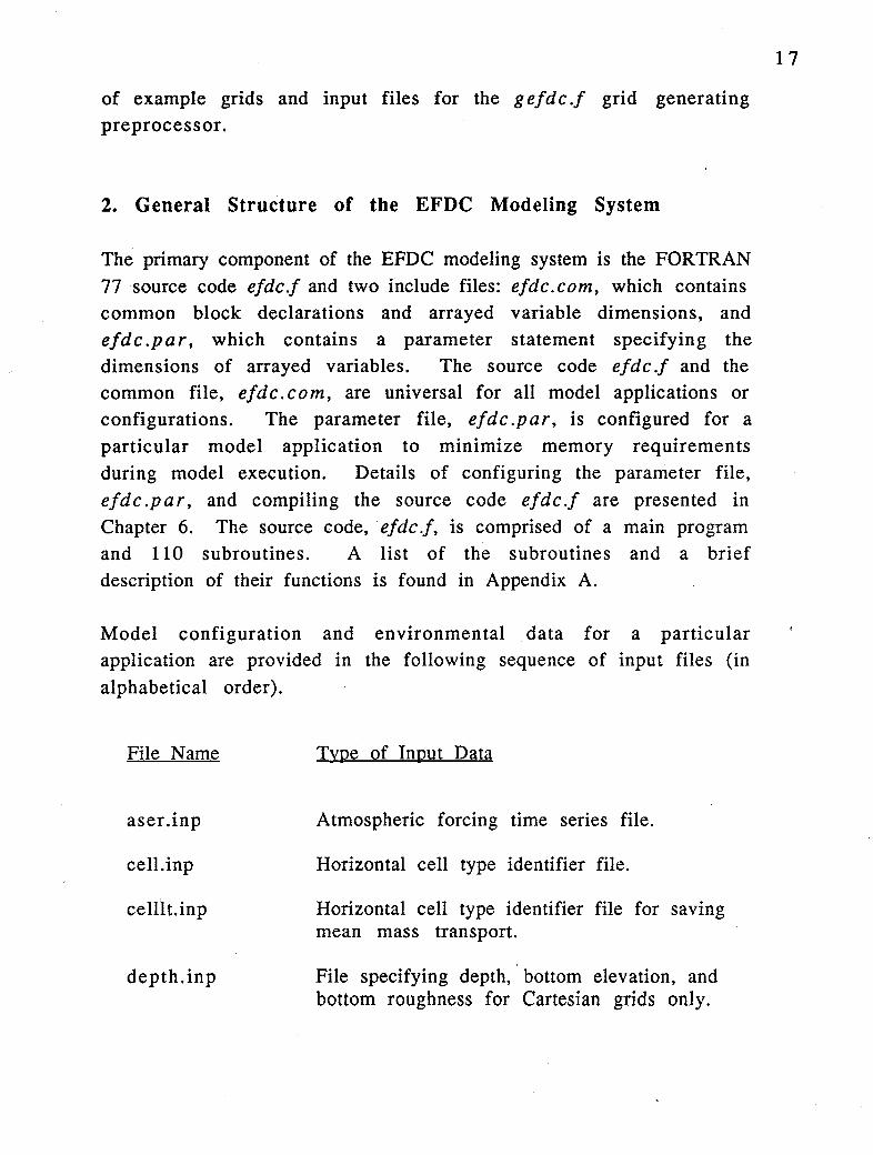
The primary component of the EFDC modeling system is the FORTRAN 77 source code efdc.f and two include files: efdc.com, which contains common block declarations and arrayed variable dimensions, and efdc .par, which contains a parameter statement specifying the dimensions of arrayed variables. The source code efdc .f and the common file, efdc.com, are universal for all model applications or configurations. The parameter file, efdc .par, is configured for a particular model application to minimize memory requirements during model execution. Details of configuring the parameter file, efdc.par, and compiling the source code efdc.f are presented in Chapter 6. The source code, ef de .f, is comprised of a main program and 110 subroutines. A list of the subroutines and a brief description of their functions is found in Appendix A.

Model configuration application are provided alphabetical order).

and environmental data for a particular in the following sequence of input files (in

File Name

aser.1np

cell.inp

celllt.inp

depth.inp

Type of Input Data

Atmospheric forcing time series file.

Horizontal cell type identifier file.

Horizontal cell type identifier file for saving mean mass transport.

File specifying depth, bottom elevation, and bottom roughness for Cartesian grids only.

17

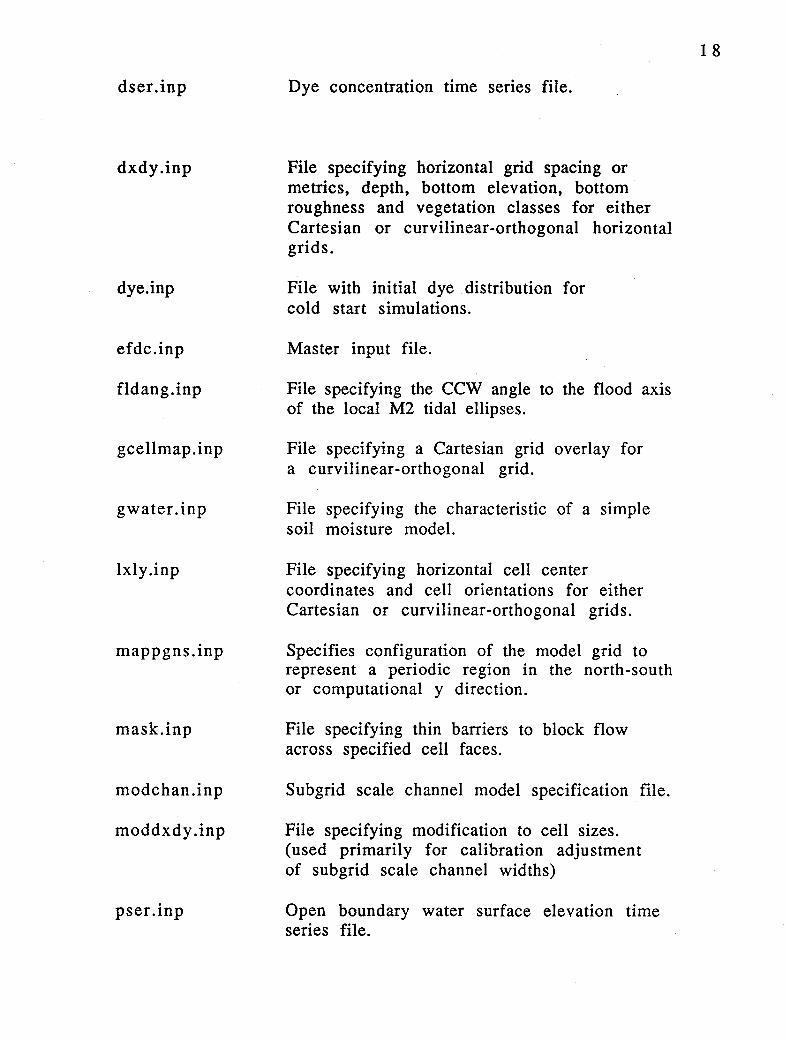
dser.inp

dxdy.inp

dye.inp

efdc.inp

fldang.inp

gcellmap.inp

gwater.inp

lxly .inp

mappgns.inp

mask.inp

modchan.inp

moddxdy .inp

pser.1np

Dye concentration time series file.

File specifying horizontal grid spacing or metrics, depth, bottom elevation, bottom roughness and vegetation classes for either Cartesian or curvilinear-orthogonal horizontal grids.

File with initial dye distribution for cold start simulations.

Master input file.

File specifying the CCW angle to the flood axis of the local M2 tidal ellipses.

File specifying a Cartesian grid overlay for a curvilinear-orthogonal grid.

File specifying the characteristic of a simple soil moisture model.

File specifying horizontal cell center coordinates and cell orientations for either Cartesian or curvilinear-orthogonal grids.

Specifies configuration of the model grid to represent a periodic region in the north-south or computational y direction.

File specifying thin barriers to block flow across specified cell faces.

Subgrid scale channel model specification file.

File specifying modification to cell sizes. (used primarily for calibration adjustment of subgrid scale channel widths)

Open boundary water surface elevation time series file.

18

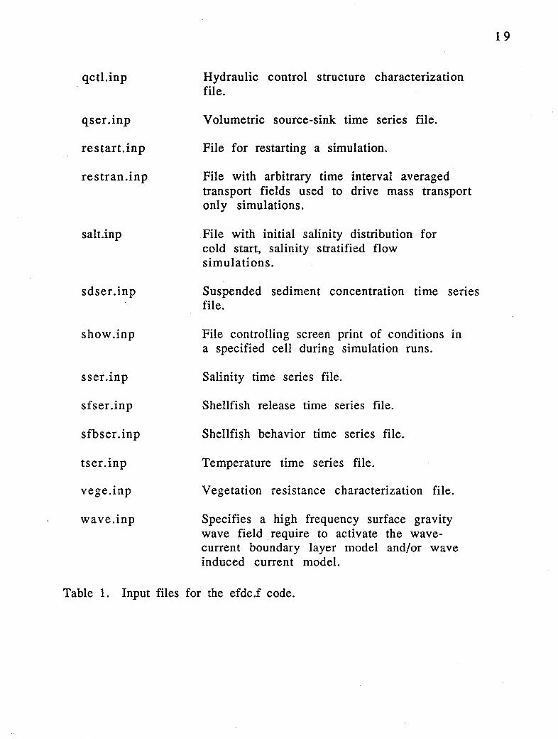
qctl.inp

qser.inp

restart.inp

restran.inp

salt.inp

sdser .inp

show.inp

sser .1np

sfser .inp

sfbser.inp

tser .inp

vege.1np

wave.inp

Hydraulic control structure characterization file.

Volumetric source-sink time series file.

File for restarting a simulation.

File with arbitrary time interval averaged transport fields used to drive mass transport only simulations.

File with initial salinity distribution for cold start, salinity stratified flow simulations.

Suspended sediment concentration time series file.

File controlling screen print of conditions m a specified cell during simulation runs.

Salinity time series file.

Shellfish release time series file.

Shellfi~h behavior time series file.

Temperature time series file.

Vegetation resistance characterization file.

Specifies a high frequency surface gravity wave field require to activate the wavecurrent boundary layer model and/or wave induced current model.

Table 1. Input files for the efdc.f code.

19

The above listed input files can be classified in four groups as follows.

1. Horizontal grid specification files:

cell.inp depth.inp gcellmap.:inp mappgns.inp

celllt.inp dxdy.inp lxly .inp mask.inp

2. General data and run control files:

efdc.inp show.inp

3. Initialization and restart files:

salt.inp dye.inp restart.inp restran.inp

4. Physical process specification files:

gwater.inp modchan.inp

5.

moddxdy .inp vege.inp

Time series

aser.inp pser.inp sdser .inp sfbser .inp sser .inp

forcing

qctl.inp wave.inp

and boundary

dser.inp qser.inp sfser .inp sser .inp

condition files:

Table 2. Input files grouped by function.

20

The recommended sequence for the construction of the input files for configuration of the model and set up for a simulation generally corresponds to the above file group classes. The files, dxdy. i np and Ix ly. i np, which specify the model grid geometry and topography or bathymetry, and the file, gcellmap.inp, which specifies an optional graphics overlay grid, can be automatically generated by an auxiliary grid generating preprocessor code GEFDC (FORTRAN 77 source file g ef de./). The use of GEFDC is discussed in Chapter 3. The master input file, efdc. inp, is discussed in detail in Chapter 4, while the structure of the remaining input files are described in Chapter 5.

The EFDC modeling system produces five classes of output: 1) diagnostic output files; 2) restart and transport field files; 3) time series, point samples and least squares harmonic analysis output files; 4) two-dimensional graphics and visualization files; and 5) three-dimensional graphics and visualization files. The activation and control of these output classes is specified in the master input file ef d c. i np, as will be discussed in Chapter 4. Guidance for activating and analyzing diagnostic output options is discussed in Chapter 7, while Chapters 8, 9, and 10 describe the formats and processing procedures for time series, two-dimensional and threedimensional model outputs.

21

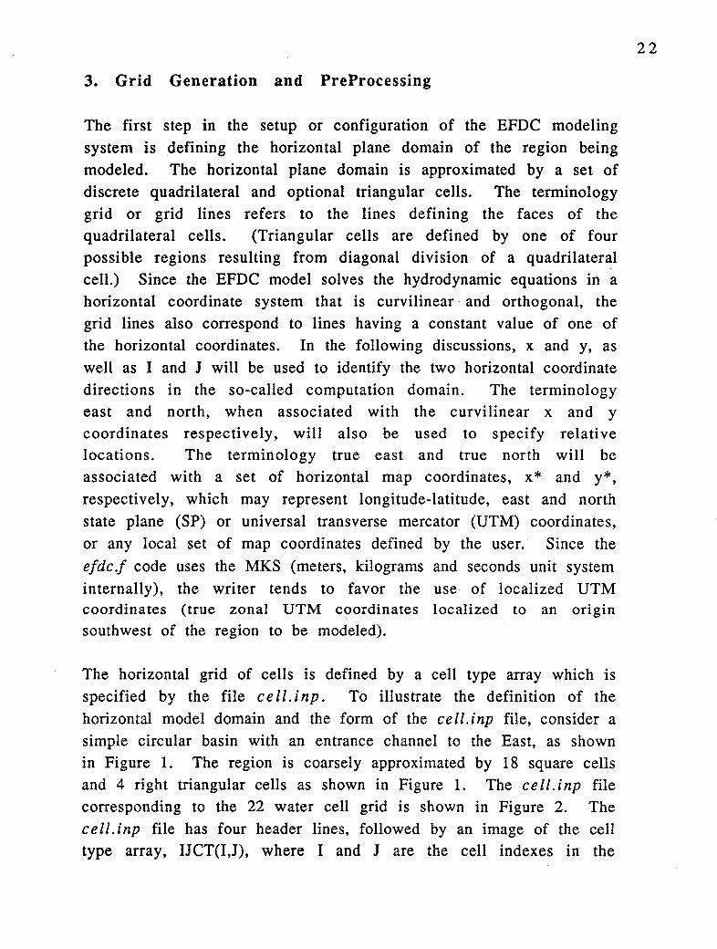
3. Grid Generation and PreProcessing

The first step in the setup or configuration of the EFDC modeling system is defining the horizontal plane domain of the region being modeled. The horizontal plane domain is approximated by a set of discrete quadrilateral and optional triangular cells. The terminology grid or grid lines refers to the lines defining the faces of the quadrilateral cells. (Triangular cells are defined by one of four possible regions resulting from diagonal division of a quadrilateral cell.) Since the EFDC model solves the hydrodynamic equations in a horizontal coordinate system that is curvilinear and orthogonal, the grid lines also correspond to lines having a constant value of one of the horizontal coordinates. In the following discussions, x and y, as well as I and J will be used to identify the two horizontal coordinate directions in the so-called computation domain. The terminology east and north, when associated with the curvilinear x and y coordinates respectively, will also be used to specify relative locations. The terminology true east and true north will be associated with a set of horizontal map coordinates, x * and y*, respectively, which may represent longitude-latitude, east and north state plane (SP) or universal transverse mercator (UTM) coordinates, or any local set of map coordinates defined by the user. Since the ef de .f code uses the MKS (meters, kilograms and seconds unit system internally), the writer tends to favor the use of localized UTM coordinates (true zonal UTM coordinates localized to an origin southwest of the region to be modeled).

The horizontal grid of cells is defined by a cell type array which is specified by the file cell. i np. To illustrate the definition of the horizontal model domain and the form of the cell.inp file, consider a simple circular basin with an entrance channel to the East, as shown in Figure 1. The region is coarsely approximated by 18 square cells and 4 right triangular cells as shown in Figure 1. The cell. i np file corresponding to the 22 water cell grid is shown in Figure 2. The cell. inp file has four header lines, followed by an image of the cell type array, IJCT(l,J), where I and J are the cell indexes in the

22

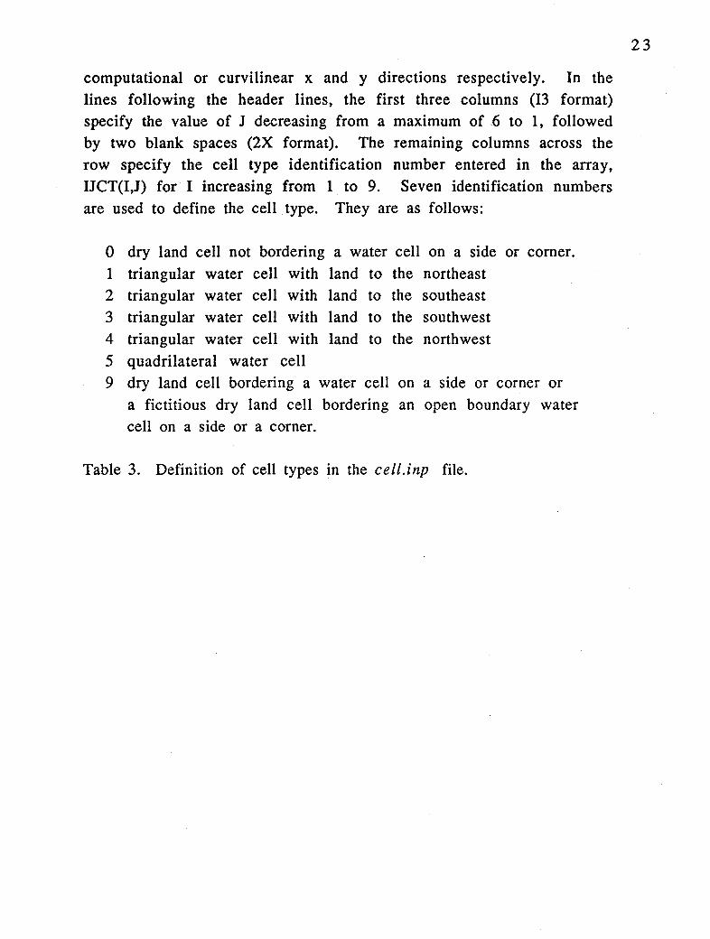
computational or curvilinear x and y directions respectively. In the lines following the header lines, the first three columns (I3 format) specify the value of J decreasing from a maximum of .6 to 1, followed by two blank spaces (2X format). The remaining columns across the row specify the cell type identification number entered in the array, IJCT(I,J) for I increasing from 1 to 9. Seven identification numbers are used to define the cell type. They are as follows:

0 dry land cell not bordering a water cell on a side or corner. 1 triangular water cell with land to the northeast 2 triangular water cell with land to the southeast 3 triangular water cell with land to the southwest 4 triangular water cell with land to the northwest 5 quadrilateral water cell 9 dry land cell bordering a water cell on a side or corner or

a fictitious dry land cell bordering an open boundary water cell on a side or a corner.

Table 3. Definition of cell types in the cell.inp file.

23

Figure 1. Representation of a circular basin and entrance channel by a 22 water cell grid.

C cell. inp file, i columns and j rows, for Figure 1 C O 1 C 1234567890 C

C

6 999999000 5 945519999 4 955555559 3 955555559 2 935529999 1 999999000

C 1234567890 C O 1

Figure 2. File cell.inp corresponding to the grid shown in Figure 1.

24

C celllt.inp file, i columns and j rows, for Figure 1 C O 1 C 1234567890 C

C

6 999999000 5 945519900 4 955555900 3 955555900 2 935529900 1 999999000

C 1234567890 C O 1

Figure 3. File celllt.inp corresponding to the cell.inp file shown m Figure 1, with four entry channel cells removed.

The type 9 dry land or fictitious dry land cell type is used in the specification of no flow boundary conditions and in graphics masking operations. For purposes of assigning adjacent type 9 cells, triangular water cells are treated identically to quadrilateral water cells. The file celllt.inp may be identical to the file cell.inp or specify a subset of the water cells in the cell.inp file. In specifying the subset, the following rules apply. Type O cells remain unchanged, type 9 cells may be changed only to type 0, and type 1 ~5 cells may be changed only to types O or 9. Figure 3 illustrates a celllt.inp file corresponding to the cell.inp file in Figure 2 with four of the entry channel cells removed.

To specify the horizontal geometric and topographic properties and other related characteristics of the region, the files dx dy. i np and lx ly. i np are preferably used. (An older model option used the depth.inp file for this purpose. However this is not recommended). For this simple grid, these files, shown in Figure 4 and 5, can be readily constructed by hand. Both files, which are read into the model execution in free format, begin with four header lines defining the columns. The file dxdy. i np provides the physical x and y

dimensions of a cell, dx and dy, the initial water depth, the bottom

25

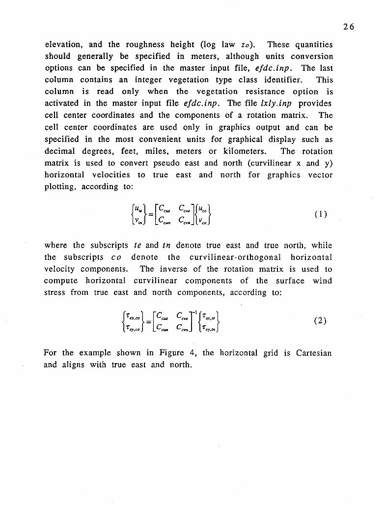
elevation, and the roughness height (log law zo ). These quantities should generally be specified in meters, although units conversion options can be specified in the master input file, efdc.inp. The last column contains an integer vegetation type class identifier. This column is read only when the vegetation resistance option is activated in the master input file efdc.inp. The file lxly.inp provides cell center coordinates and the components of a rotation matrix. The cell center coordinates are used only in graphics output and can be specified in the most convenient units for graphical display such as decimal degrees, feet, miles, meters or kilometers. The rotation matrix is used to convert pseudo east and north ( curvilinear x and y) horizontal velocities to true east and north for graphics vector plotting, according to:

(1)

where the subscripts te and tn denote true east and true north, while the subscripts co denote the curvilinear-orthogonal horizontal velocity components. The inverse of the rotation matrix is used to compute horizontal curvilinear components of the surface wind stress from true east and north components, according to:

{-r.U:,CO} = [CCIU cm]-l{"S%,I~} '"( sy,co Cc.,,,. C cv11 '"C sy,111

(2)

For the example shown in Figure 4, the horizontal grid 1s Cartesian and aligns with true east and north.

26

27

C dxdy. inp file, in free format across colUITU1s C C I J DX DY DEPTH BOTTCM ELEV ZROUGH VEG TYPE C

2 2 100.0 100.0 5.0 -5.0 0.02 0 3 2 100.0 100.0 5.0 -5.0 0.02 0 4 2 100.0 100.0 5.0 -5.0 0.02 0 5 2 100.0 100.0 5.0 -5.0 0.02 0 6 2 100.0 100.0 5.0 -5.0 0.02 0 7 2 100.0 100.0 5.0 -5.0 0.02 0 8 2 100.0 100.0 5.0 -5.0 0.02 0 2 3 100.0 100.0 5.0 -5.0 0.02 0 3 3 100.0 100.0 5.0 -5.0 0.02 0 4 3 100.0 100.0 5.0 -5.0 0.02 0 5 3 100.0 100.0 5.0 -5.0 0.02 0 6 3 100.0 100.0 5.0 -5.0 0.02 0 7 3 100.0 100.0 5.0 -5.0 0.02 0 8 3 100.0 100.0 5.0 -5.0 0.02 0 2 4 100.0 100.0 5.0 -5.0 0.02 0 3 4 100.0 100.0 5.0 -5.0 0.02 0 4 4 100.0 100.0 5.0 -5.0 0.02 0 5 4 100.0 100.0 5.0 -5.0 0.02 0 6 4 100.0 100.0 5.0 -5.0 0.02 0 7 4 100.0 100.0 5.0 -5.0 0.02 0 8 4 100.0 100.0 5.0 -5.0 0.02 0 2 5 100.0 100.0 5.0 -5.0 0.02 0 3 5 100.0 100.0 5.0 -5.0 0.02 0 4 5 100.0 100.0 5.0 -5.0 0.02 0 5 5 100.0 100.0 5.0 -5.0 0.02 0 6 5 100.0 100.0 5.0 -5.0 0.02 0 7 5 100.0 100.0 5.0 -5.0 0.02 0 8 5 100.0 100.0 5.0 -5.0 0.02 0

C C I ARRAY INDEX IN X DIRECTION C J ARRAY INDEX IN Y DIRECTION C DX CELL DIMENSION IN X DIRECTION, METERS C DY CELL DIMENSION IN Y DIRECTION, METERS C DEPTH INITIAL WATER DEPTH, METERS C J30TTOM ELEV J30TTOM BED ELEVATION, METERS C ZROUGH LOG LAW ROUGHNESS HEIGHI', ZO, METERS C VEG TYPE VEGETATION TYPE CLASS, INTEGER VALUE C

Figure 4. File dxdy.inp for grid shown in Figure 1.

28

C lxly.inp file, in free format across columns C C I J XINU™E YL~ CCUE CCVE CCON CCVN C

2 2 250.0 250.0 1.0 0.0 0.0 1.0 3 2 350.0 250.0 1.0 0.0 0.0 1.0 4 2 450.0 250.0 1.0 0.0 0.0 1.0 5 2 550.0 250.0 1.0 0.0 0.0 1.0 6 2 650.0 250.0 1.0 0.0 0.0 1.0 7 2 750.0 250.0 1.0 0.0 0.0 1.0 8 2 850.0 250.0 1.0 0.0 0.0 1.0 2 3 250.0 350.0 1.0 0.0 0.0 1.0 3 3 350.0 350.0 1.0 0.0 0.0 1.0 4 3 450.0 350.0 1.0 0.0 0.0 1.0 5 3 550.0 350.0 1.0 0.0 0.0 1.0 6 3 650.0 350.0 1.0 0.0 0.0 1.0 7 3 750.0 350.0 1.0 0.0 0.0 1.0 8 3 850.0 350.0 1.0 0.0 0.0 1.0 2 4 250.0 450.0 1.0 0.0 0.0 1.0 3 4 350.0 450.0 1.0 0.0 0.0 1.0 4 4 450.0 450.0 1.0 0.0 0.0 1.0 5 4 550.0 450.0 1.0 0.0 0.0 1.0 6 4 650.0 450.0 1.0 0.0 0.0 1.0 7 4 750.0 450.0 1.0 0.0 0.0 1.0 8 4 850.0 450.0 1.0 0.0 0.0 1.0 2 5 250.0 550.0 1.0 0.0 0.0 1.0 3 5 350.0 550.0 1.0 0.0 0.0 1.0 4 5 450.0 550.0 1.0 0.0 0.0 1.0 5 5 550.0 550.0 1.0 0.0 0.0 1.0 6 5 650.0 550.0 1.0 0.0 0.0 1.0 7 5 750.0 550.0 1.0 0.0 0.0 1.0 8 5 850.0 550.0 1.0 0.0 0.0 1.0

C C C I ARRAY INDEX IN X DIRECTION C J ARRAY INDEX IN Y DIRECTION C XLNUTME X CEIL CENTER COORDINATE, I.ONGITUDE, METERS, OR KM C YLTUTMN Y CEIL CENTER COORDINATE, I.ONGITUDE, METERS, OR KM C CCUE ROTATION MATRIX COMPONENT C CCVE ROTATION MATRIX COMPONENT C CCON ROTATION MATRIX COMPONENT C CCVN ROTATION MATRIX COMPONENT C

Figure 5. File lxly.inp for grid shown in Figure 1.

For realistic model applications, the grid generating preprocessor code, gefdc.f, is used to generate the horizontal grid and form the dxdy.inp and lxly.inp files. The gefdc.f code requires the following input files:

cell.inp

depdat.inp

gcell.inp

gridext.inp

gefdc.inp

vege.inp

zrough.inp

Cell type file as in Figure 2.

File specifying depth or bottom topography ( optional if depth interpolation is not specified).

Optional auxiliary file with cell. inp format which specifies an auxiliary square Cartesian grid for rectangular array graphics when the actual computational grid is curvilinear.

File of water cell corner coordinates for used with NTYPE = 0 grid generation option.

Master input file for gefdc.f.

File specifying vegetation type classes.

File specifying bottom roughness (log law zo).

Table 4. Input files for the gefdc.f grid generating preprocessor.

The format of the cell.inp file has already been discussed. The depdat. inp file is a three column ASCII text file with no header, as shown in Figure 6. The first two columns are true east and true north coordinates, in meters or kilometers, with the depth or bottom elevation given in the third column. The origin of the true east and north coordinates is arbitrary, but should generally be related to an accepted geographic coordinate system such as longitude-latitude, state plane, or universal transverse mercator. The optional file gcell.inp has the same format as the cell.inp file, but specifies an auxiliary, square cell, Cartesian grid corresponding to the curvilinear grid specified by the cell. inp file. When the option to process the

29

geell.inp file is activated in the gefde.inp file, a correspondence table between the curvilinear grid and the auxiliary, square cell, Cartesian grid is generated. The correspondence table, output as file geellmap.inp, is used by the efde.f code to generated two and threedimensional rectangular arrays of graphics visualization, as will be subsequently discussed. The file gridext.inp is used for generation of a grid constructed external to the g ef de .f code. This file is a four column free format ASCII text file with no header. The four columns correspond to the I indices, J indices, true east coordinates, and true north coordinates of the water cell corners. The lower left (pseudo southwest relative to the cell center) cell corners carry the same I and J indices as the cell. The gridext.inp file corresponding to the simple grid in Figure 1 is shown in Figure 7. Triangular cells must be specified as equivalent quadrilaterals in the gridext. inp file. The files vege.inp and zrough.inp have the same format as the depdat.inp file, with the exception that the third column of the vege.inp file has an integer value corresponding to a vegetation class. The third column of the zrough.inp file has values of the log law bottom roughness height, zo, (preferably in meters, however unit conversion may be specified in the master input file ef de .f).

4.2798 4.2785 4.4509 4.4409 4.4222 4.4133

6.9175 6.9175 6.7880 6. 7927 6.7995 6.8028

3.2309 3.2309 3.1090 3.1090 3.1090 3.1090

Figure 6. Format of the file depdat.inp.

30

3 1

2 2 200. 200. 3 2 300. 200. 4 2 400. 200. 5 2 500. 200. 6 2 600. 200. 2 3 200. 300. 3 3 300. 300. 4 3 400. 300. 5 3 500. 300. 6 3 600. 300. 7 3 700. 300. 8 3 800. 300. 9 3 900. 300. 2 4 200. 400. 3 4 300. 400. 4 4 400. 400. 5 4 500. 400. 6 4 600. 400. 7 4 700. 400. 8 4 800. 400. 9 4 900. 400. 2 . 5 200. 500 . 3 .5 300 . 500. 4 .5 400. 500 . 5 .5 500 . 500. 6 .5 600. 500. 7 .5 700. 500 . 8 5 800. 500. 9 .5 900. 500 . 2 6 200. 600. 3 6 300. 600. 4 6 400. 600. 5 6 500. 600. 6 6 600. 600.

Figure 7. File gridext.inp for grid shown in Figure 1.

Cl TITIE Cl (LIMITED TO 80 CHARACTERS)

'gefdc.inp corresponding to exarrple in figure 1' C2 INTEGER INPUT

· C2 NTYPE NBPP IMIN IMAX JMIN JMAX IC JC 0 0 1 9 1 6 9 6

C3 GRAPHICS GRID INFORMATION C3 ISGG IG1 JG1 DXCG DYCG NWTGG

0 0 0 0. 0. 1 C4 CARTESIAN AND GRAPHICS GRID COORDINATE DATA C4 CDLONl CDI.CN2 CDLON3 CDLATl CDLAT2 CDIAT3

0. 0. 0. 0. 0. 0. CS INTEGER INPUT CS ITRXM ITRHM ITRKM ITRG1 NDEPSM DEPMIN

100 100 100 100 4000 1.0 C6 REAL INPUT C6 RPX RPK RPH RSQXM RSQKM RSQKIM RSQHM RSQHIM RSQHJM

1.8 1.8 1.8 1.E-12 1.E-12 1.E-12 1.E-12 1.E-12 1.E-12 C7 COORDINATE SHIFT PA.RAMETERS C7 XSHIFT YSHIFT HSCALE RK..JDKI ANGORO

0 . 0 . 1. 1. 15. 0 C8 INTERPOLATION SWITCHES C8 ISIRKI JSIRKI ISIHIHJ JSIHIHJ

1 0 0 0 C9 NTYPE = 7 SPECIFID INPUT C9 IB IE JB JE N7RLX NXYIT ITN7M IJSMD ISMD JSMD RP7 SERRMAX Cl O NTYPE = 7 SPECIFID INPUT ClO X Y IN ORDER (IB,JB) (IE,JB) (IE,JE) (IB,JE) Cll DEPTH INTERPOLATION SWITCHES Cll ISIDEP NDEPDAT CDEP RADM ISIDPTYP SURFELV ISVEG NVEGDAT NVEGTYP

0 0 2 .. 5 2 4.0 0 0 0 Cl2 LAST BCUNDARY POINT INFORMATION Cl2 ILT JLT X(ILT,JLT) Y(ILT,JLT)

1 1 0. 0. Cl3 BOUNDARY POINT INFORMATION Cl3 I J X(I,J) Y(I,J)

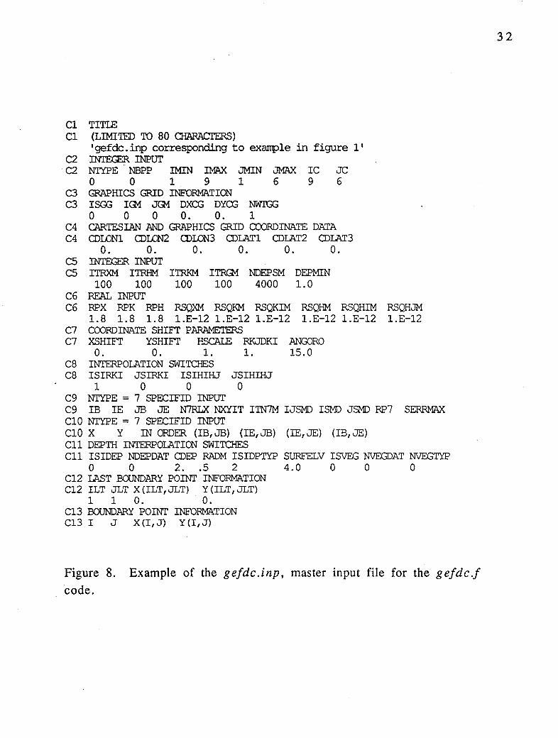
Figure 8. Example of the gefdc.inp, master input file for the gefdc.f

code.

32

The execution of the gefdc.f code is controlled by its master input file, gefdc.inp. An example of the gefdc.inp file for the grid in Figure 1 is shown in Figure 8. The file is essentially a sequence of 'card images' or input lines. Each input line is preceded by card number lines beginning with 'C' followed by a number corresponding the card image or data input line and text defining the data type and the actual data parameters. To fully discuss the options in the execution of the gefdc.f code, it is useful to consider each 'card image' or input line sequence. The following discussion will sequentially present the header and data lines in Monaco text with definitions of data parameters following in Monaco text. Additional discussion then follows in plain text. In the discussions, reference will be made to six grid generation examples in Appendix B, which illustrate specific options as well as showing the resulting grid.

Card Image 1

Cl TITI.E Cl (LIMITED TO 80 CHARACTERS)

'ENR GRID'

The 80 character title simply serves to identify the particular application.

33

Card Image 2

C2 INTEGER INPUT C2 NTYPE NBPP !MIN IMAX JMIN JMAX IC JC

0 0 1 50 1 55 50 55

Card Image 2 Parameter Definitions

NTYPE = PROBIEM TYPE 0, READ IN FIIE 'cell. inp' AND WATER GRID CELL CORNER

COORDINATES FRCM FIIE 'gridext. inp' TO GENERA'IE INPUT FIIES FOR AN EXTERNALLY GENERA'IED ORTHCGCNAL GRID

1-,5 GENERATE AN ORTHCGONAL GRID AND INPUT FIIES

USING THE METHOD OF RYSKIN AND LEAL, J. OF CCMP. PHYS. VSO, 71-100 (1983) WITH SYM1ETRIC REFIECTIONS AS SUGGESTED BY CHIKHLIWAI.A AND YORTSOS, J. OF CCMP. PHYS. V57, 391-402 (1985).

1, RL-CY EAST REFIECTION 2, RL-CY NORTH REFIECTION 3, RL-CY WEST REFIECTION 4, RL-CY SOUTH REFIECTION 5, RL NO REFIECTION 6, GENERA'IE GRID AND INPUT FIIES USING

THE AREA-ORTHCGONALITY METHOD OF KNUPP, J. OF CCMP PHYS. VlOO, 409-418 (1993) ORTHCGONALITY IS Nor GUARANTEED

7, GENERATE GRID ORTHCGONAL GRID AND INPUT FIIES USING THE QUASI-CONFORMAL METHOD OF M:>BIEY AND STEWART, J. OF CCMP PHYS. V24, 124-135 (1980) REQUIRES USER SUPPLIED FUNCTION SUBROUTINES FIB,FIE,GJB,GJE

8, DEPTH INTERPOLATION TO CARTESIAN GRID SPECIFIED BY cell.inp AND GENERATE dxdy.inp AND lxly.inp FilES

9, DEPTH IN'IERPOIATICN TO CARTESIAN GRID AS FOR 8 CCNVERTING INPUT COORDINA'IE SYSTEM FRCM LONG, IAT TO UTMBAY (VIMS PHYS OCEAN CHES BAY REF)

NBPP = NUMBER OF INPUT BOUNDARY POINTS (Nl'YPE = 1-6) IMIN,IMAX = RANGE OF I GRID INDICES JMIN,JMAX = RANGE OF J GRID INDICES IC= NUMBER OF CELLS IN I DIRECTION JC= NUMBER OF CELLS IN J DIRECTION

34

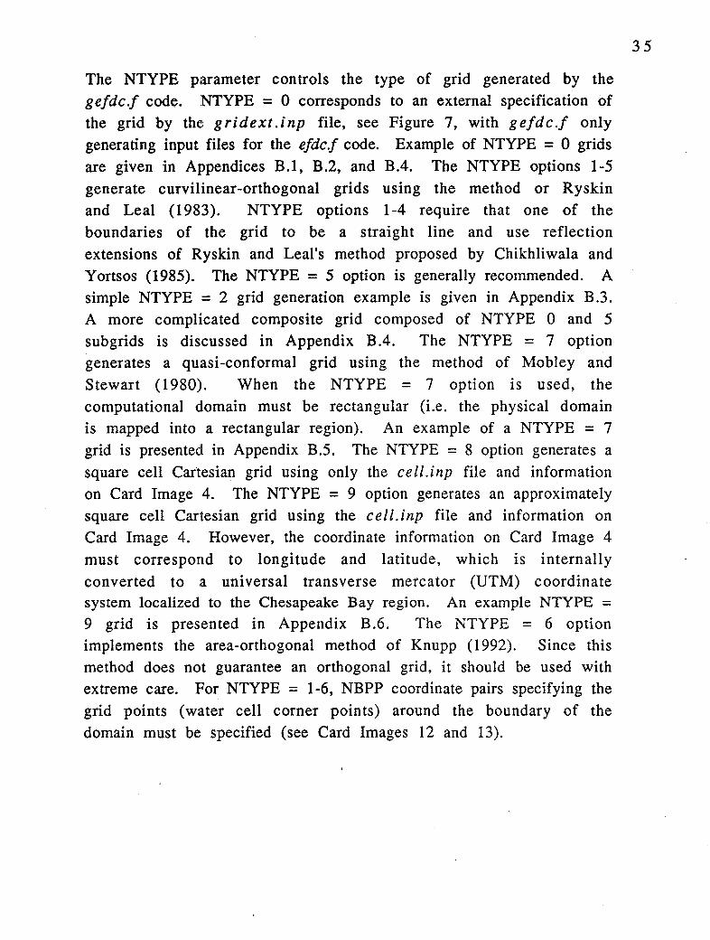
The NTYPE parameter controls the type of grid generated by the gefdc.f code. NTYPE = 0 corresponds to an external specification of the grid by the gridext.inp file, see Figure 7, with gefdc.f only generating input files for the efdc.f code. Example of NTYPE = 0 grids are given in Appendices B.1, B.2, and B.4. The NTYPE options 1-5 generate curvilinear-orthogonal grids using the method or Ryskin and Leal (1983). NTYPE options 1-4 require that one of the boundaries of the grid to be a straight line and use reflection extensions of Ryskin and Leal's method proposed by Chikhliwala and Yortsos (1985). The NTYPE = 5 option is generally recommended. A simple NTYPE = 2 grid generation example is given in Appendix B.3. A more complicated composite grid composed of NTYPE O and 5 subgrids is discussed in Appendix B.4. The NTYPE = 7 option generates a quasi-conformal grid using the method of Mobley and Stewart (1980). When the NTYPE = 7 option is used, the computational domain must be rectangular (i.e. the physical domain is mapped into a rectangular region). An example of a NTYPE = 7 grid is presented in Appendix B.5. The NTYPE = 8 option generates a square cell Cartesian grid using only the cell.inp file and information on Card Image 4. The NTYPE = 9 option generates an approximately square cell Cartesian grid using the cell.inp file and information on Card Image 4. However, the coordinate information on Card Image 4 must correspond to longitude and latitude, which is internally converted to a universal transverse mercator (UTM) coordinate system localized to the Chesapeake Bay region. An example NTYPE = 9 grid is presented in Appendix B.6. The NTYPE = 6 option implements the area-orthogonal method of Knupp (1992). Since this method does not guarantee an orthogonal grid, it should be used with extreme care. For NTYPE = 1-6, NBPP coordinate pairs specifying the grid points (water cell corner points) around the boundary of the domain must be specified (see Card Images 12 and 13).

35

Card Image 3

C3 GRAPHICS GRID INFORMATION C3 ISGG IQ.f JG1 DXCG DYCG NWIGG

0 0 0 1. 1. 1


ISGG = 1, READ IN gcell.inp WHICH DEFINES THE CARTESIAN OR

IQ.f JG1 DXCG DYCG NWI'GG

GRAPHICS GRID OVERIAY MAXIMUM XOR I CELLS IN CARTESIAN OR GRAPHICS GRID MAXIMUM Y OF J CELLS IN CARTESIAN OR GRAPHICS GRID X GRID SIZE OF CARTESIAN OR GRAPHICS GRID Y GRID SIZE OF CARTESIAN OF GRAPHICS GRID NUMBER OF WEIGHTED COw11? CELLS USED TO INI'ERPOIATE TO THE GRAPHICS GRID {MUST EQUAL 1)

Activation of ISGG = 1, allows for a square cell Cartesian grid to be simultaneously generated when NTYPE = 1-7. This Cartesian grid is used by efdc .f to output the results of a 30 curvilinear coordinate computation in a 3D rectangular array for visualization and graphics. The relation between the I and J indices of the Cartesian grid, specified by gcell.inp, and the global coordinates (true east and true north) defining the curvilinear grid in physical space are defined by input on Card Image 4. The gcell.inp file has the same format as the cell.inp file. The gefdc.inp files shown in Figure BI4 and B27 are examples where the ISGG = 1 option is activated.

36

Card Image 4

C4 CARTESIAN AND GRAPHICS GRID CXX)RI)INATE DATA C4 CDI.ONl CDLON2 CDI.ON3 CDIATl CDIAT2 CDLAT3

-77.5 1.25 -0.625 36.7 1.0 -0.5


CDI.ONl: CDI.ON2: CDI.ON3: CDIATl: CDIAT2: CDIAT3:

6 CONSTANTS TO GIVE CELL CENTER IAT AND LON OR OTHER COORDINATES FOR CARTESIAN GRIDS USING THE FORMUI.AE DLCN(L)=CDLONl+(CDLON2*FLOAT(I)+a)LON3)/60. DLAT(L)=CDIAT1+(CDIAT2*FLOAT(J)+a)IAT3)/60.

The information on this card image defines the global coordinates (true east and true north) of Cartesian cell centers corresponding to the I and J indices in the gcell.inp file for the Cartesian graphics grid overlay when NTYPE = 1-7 is specified (see gefdc.inp files in Figure B 14 and B27). When NTYPE = 8 or 9 is specified, the information defines the cell center coordinates corresponding to I and J indices in the cell.inp file (see the gefdc.inp file in Figure B34). When NTYPE =

9, DLON and DLAT must correspond to longitude and latitude, otherwise DLON and DLA T can also correspond to a true east and true north coordinate system in meters or kilometers.

37

Card Image 5

CS INTEGER INPUT CS ITRXM ITRHM ITRKM ITRG1 NDEPSM DEPMIN

500 500 500 500 4000 1.0


ITRXM = :MAXIM.JM NUMBER OF X,Y SOLUTION ITERATICNS ITRHM = :MAXIM.JM NUMBER OF HI,HJ SOLUTION ITERATICNS ITRKM = :MAXIMJM NUMBER OF KJ/KI SOLUTION ITERATICNS ITRG1 = :MAXIM.JM NUMBER OF GRID SOLUTION ITERATICNS NDEPSM = NUMBER SMX>THING PASSES TO FILL MISSING DEP DAT DEPMIN = MINIMUM DEPTH PASSING DEPDAT. INP DATA

The first four parameters on Card Image 5 control the number of iterations for the various curvilinear grid generation schemes, based on successive over relaxation (SOR) solutions of elliptic equations, in gefdc.f. The value of 500 is recommended as a maximum for each of the these parameters based on the writer's experience that if the successive over relaxation (SOR) solution schemes do not converge after 500 iterations they are not converging at all. The value of 4000 for NDEPSM is the recommended number of smoothing passes used to fill in missing depth or bottom elevation data when the ISIDEP = 1 option on Card Image 11 is activated.

38

Card Image 6

C6 REAL INPUT C6 RPX RPK RPH RSQXM RSQKM RSQKIM RSQHM RSQHIM RSQHJM

1.8 1.8 1.8 1.E-12 1.E-12 1.E-12 l.E-12 l.E-12 l.E-12

Card Image 6 Parameter Definitions·

RPX,RPK,RPH = REIAXATION PARAMETERS FOR X, Y; KI/KJ; AND HI,HJ SOR SOLUTICNS

RSQXM,RSQKM,RSQHM = MAXIMUM RESIDUAL SQUARED ERROR IN SOR SOLUTICN FOR X,Y; KJ/KI; AND HI,HJ

RSQKIM = CONVERGENCE CRITERIA BASED ON KI/KJ (NOT ACTIVE) RSQHIM = CONVERGENCE CRITERIA BASED ON HI (NOT ACTIVE) RSQHJM = CONVERGENCE CRITERIA BASED ON HJ (NOT ACTIVE)

The values of the first three parameters should not be changed, since they have been determined to the near optimum for the SOR solution schemes in gefdc.f. The remaining parameters are residual squared error criteria for stopping the SOR solutions. The values shown are rough estimates. For very large grids they can be decreased in magnitude to approximately 1.E-6.

39

Card Image 7

C7 COORDINATE SHIFT PARAMETERS AND ANGULAR ERROR C7 XSHIFT YSHIFT HSCALE RK.JDKI ANGORO

0. 0. 1000. 1. 5.0


XSHIFT,YSHIFT = X,Y COORDINATE SHIFT X,Y=X,Y+XSHIFT,YSHIFT HSCALE = SCALE FACTOR FOR HII AND HJJ WHEN PRINrED TO dxdy.out RK.JDKI = ANISOTROPIC STRETCHING OF J COORDINATE (USE 1.) .NmRO = ANGULAR DEVIATION FRCM ORTHcx:;oNALITY IN DEG USED

AS CONVERGENCE CRITERIA

The first two parameters allow for a coordinate translation of input coordinate data, which is generally not recommended. The scale factor is used to convert the input coordinate units to meters. For example, if the input coordinates are in kilometers, 1000 is necessary for DX and DY in the dxdy.inp file to be properly specified in meters. Note the cell center coordinates in the lxly.inp file will remain in the same units as the input coordinates. The final parameter, ANGORO, specifies the maximum deviation from orthogonal in the final grid. If the specified maximum deviation is not achieved, the generation procedure will execute the maximum number of iterations.

40

Card Image 8

ca INTERPOIATION SWITCHES ca !SIRK! JSIRKI ISIHIHJ JSIHIHJ

1 0 0 0


!SIRK!= 1, SOLUTION BASED CN INTERPOIATION OF KJ/KI TO INI'ERIOR

JSIRKI = 1, INTERPOIATE KJ/KI TO INTERIOR WITH CONSTANI' COEFFICIENT DIFFUSION EQUATION

ISIHIHJ =1, SOLUTION BASED ON INTERPOIATION OF HI AND HJ TO INTERIOR, AND THEN DETERMINING KJ/KI=HI/HJ

JSIHIHJ = 1, INTERPOIATE HI AND HJ TO INTERIOR WITH CONSTANI' COEFFICIENT DIFFUSION EQUATION

The shown configuration for this Card Image 1s recommended.

41

Card Image 9

C9 NTYPE = 7 SPECIFIED INPUT C9 IB IE JB JE N7RLX NXYIT ITN7M IJSMD ISMD JSMD RP7 SERRMAX


IB = BEGINNIN3 I INDEX MS METHOD IE = ENDING I INDEX MS METHOD JB = BEGINNIN3 J INDEX MS METHOD JE = ENDING J INDEX MS METHOD N7REI.AX= MAXIMJM RELAXATICN PER INIT L(X)P, NTYPE = 7 NXYIT = NUMBER OF ITERS ON EACH X,Y SWEEP, NTYPE = 7 ITN7MAX= MAXIMUM GENERATION ITERS, NTYPE = 7 IJSMD = 1, CALCUIATE GLOBAL CONFORMAL M:IDULE ISMD = A VALUE IB.LE.ISMD.LE.IE, CALCUI.ATE CONFORMAL

MJDULE ALONG LINE I=ISMD JSMD = A VALUE JB. LE. JSMD. LE. JE, CALCUIATE CONFORMAL

MJDULE ALONG LINE J=JSMD RP7 = SOR RELAXATION PARAMETER, NTYPE = 7 SERRMAX= MAXIMUM CONFORMAL M:IDULE ERROR, NTYPE = 7

Data is necessary on this line only if NTYPE = 7. The indices IB and IE define the beginning and ending I grid lines of the rectangular (in the computational domain) grid generated by the quasi-conformal mapping technique implemented for NTYPE = 7. The indices JB and JE likewise define the beginning and ending J indices. Recommended values for the :remaining parameter in this card image are shown in Figure B27 in Appendix B.

42

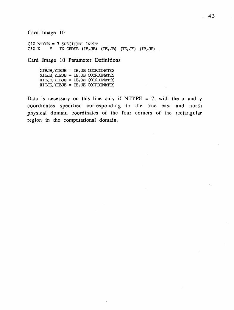
Card Image 10

ClO NI'YPE = 7 SPECIFIED INPUT ClO X Y IN OODER (IB, Jl3) (IE, JB) (IE, JE) (IB, JE)


XIBJB,YIBJB = IB,JB CXX)RD!NA'IES XIEJB,YIEJB = IE,JB CXX)RDINA'IES XIBJE,YIBJE = IB,JE CXX)RDINA'IES XIEJE,YI&JE = IE,JE CXX)RDINA'IES

Data is necessary on this line only if NTYPE = 7, with the x and y coordinates specified corresponding to the true east and north physical domain coordinates of the four corners of the rectangular region in the computational domain.

43

Card Image 11

Cll DEPTH INTERPOLATION SWI'.I'Cl1ES Cll ISIDEP NDEPDAT Q)EP RADM ISIDPTYP SURFELV ISVEG NVF.GOAT NVEGTYP

1 11564 2 .. 5 2 4.0 0 0 0


ISIDEP = 1, READ depdat.inp FIIE AND INTERPOLA'IE DEPTH, BOTTCM EI.EVATICN AND BOTTCM ROu;HNESS DATA IN THE dxdy.inp FIIB

NDEPDAT = NUMBER OF X, Y, DEPTH FIELDS IN DEPDAT.INP FilE Q)EP = WEIGHTING COEFFICIENT IN DEPTH INTERPOLATION SOIEME RN.M = CONSTANT MULTIPLIER FOR DEPTH INTERPOLATION RADIUS ISIDPTYP = 1, ASSUMES DEPDAT.INP CONTAINS POSITIVE DEPTHS

TO A BOTTCM BELOW A SEA LEVEL DATUM AND THE BOTICM EI.EVATION IS THE NEGATIVE OF THE DEPTH 2, ASSUMES DEPDAT.INP CONTAINS POSITIVE BOTTCM EI.EVATIONS, LOCAL INITIAL DEPTH rs THEN DETERMINED BY DEPTH=SURFELV-BELB 3, ASSUMES DEPDAT.INP CONTAINS POSITIVE BOTTCM EI.EVATIONS WHICH ARE CONVER'IED TO NEGATIVE VALUES, I1X:AL INITIAL DEPTH IS THEN DETERMINED BY DEPTH=SURFELV-BELB

SURFELV = INITIALLY FLAT SURFACE ELEVATION FOR USE WHEN

ISVEG NVF..ffiAT NVF..GTYP

ISIDPTYP = 2 OR 3. = 1, READ AND INTERPOLATE VEGETATION DATA = NUMBER OF X,Y,VEGETATION CLASS DATA POINTS = NUMBER OF VEGETATION TYPES OR CLASSES

Setting ISIDEP = 1 activates depth or bottom elevation interpolation

to the grid using NDEPDAT depth or bottom elevation data points. The depth or bottom elevation data within a radius of RDM*Min(dx,dy) of a cell center to determine a weighted average cell

center or cell mean depth using an inverse distance weighting if CDEP = 1 or an inverse square weighting is CDEP = 2. If no data is within RDM*Min(dx,dy) of the cell center, the cell is flagged as having missing depth or bottom elevation data. Missing depth or bottom elevation data is determined using a Laplace equation filling

technique which preserves values of the depth and bottom elevation in the unflagged cells. Vegetation class interpolation is activated by ISVEG = 1. For vegetation class interpolation, the predominant class is selected if more than on vegetation class data point falls within a

cell. Since there is no fill option for the vegetation class interpolation, cells not having vegetation data points within their

44

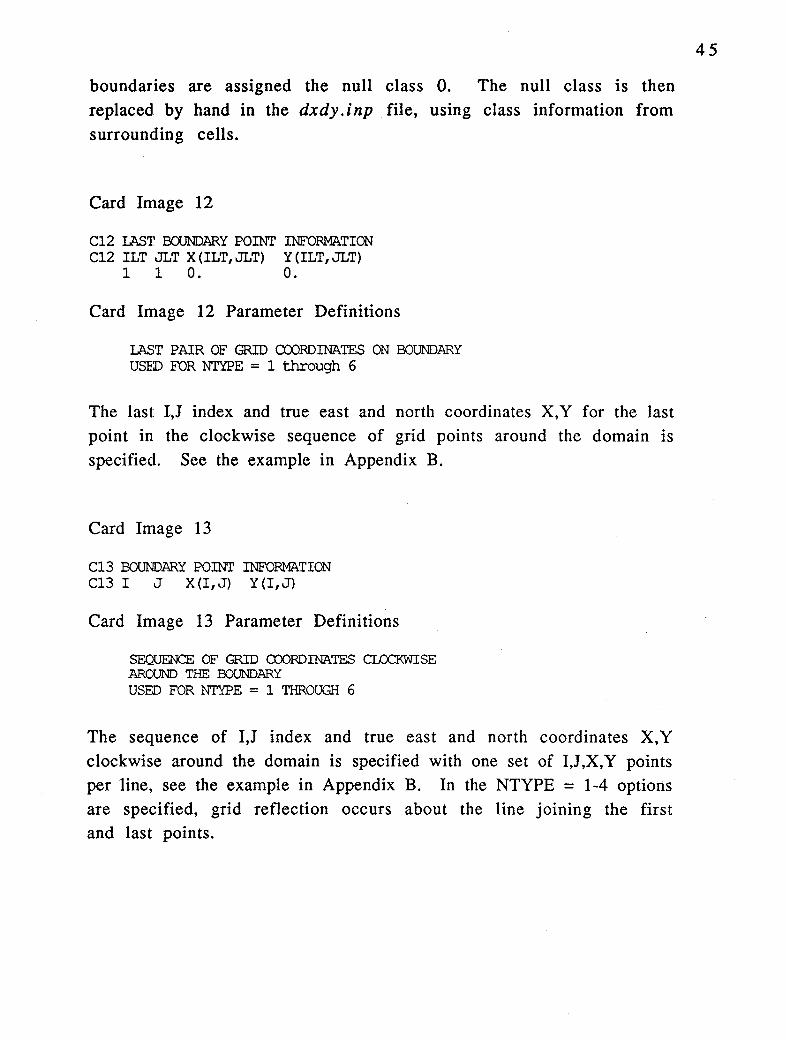
boundaries are assigned the null class 0. The null class is then replaced by hand in the dxdy. i np file, using class information from surrounding cells.

Card Image 12

Cl2 LAST BCONDARY POINT INFORMATION C12 ILT JLT X(ILT,JLT) Y(ILT,JLT)

1 1 0. 0.


LAST PAIR OF GRID COORDINATES ON BOUNDARY USED FOR NTYPE = 1 through 6

The last I,J index and true east and north coordinates X,Y for the last point in the clockwise sequence of grid points around the domain is specified. See the example in Appendix B.

Card Image 13

Cl3 BOUNDARY POINT INFORMATION Cl3 I J X (I, ~J) Y (I, J)


SEQUENCE OF GRID CTX)RDINATES CLCX:KWISE ARCUND THE BOUNDARY USED FOR NTYPE = 1 THROUGH 6

The sequence of I,J index and true east and north coordinates X,Y clockwise around the domain is specified with one set of I,J,X,Y points per line, see the example in Appendix B. In the NTYPE = 1-4 options are specified, grid reflection occurs about the line joining the first and last points.

45

The gefdc.f code generates a number of output files, including the dxdy.inp and lxly.inp files for input into the efdc.f code. {Thes,e files are actually output as dxdy.out and lxly.out and must be renamed for use by efdc.f. The other output files and their purposes and content are as follows:

depint.log

dxdy.diag

gefdc.log

gefdc.out

grid.cord

grid.dxf

A file contammg the l,J indices and true x,y coordinates of cells having no depth or bottom elevation data in their immediate vicinity ( depths and bottom elevations are determined by a smoothing interpolation).

A file · containing diagnostics for curvilinearorthogonal grids. See following text and Figure 9.

A file containing a log of the execution of the gefdc.f code. The contents of this file are also written to the screen during execution. See following text and Figure 10.

This contain a listing of the cell.inp file, the KSGI array specifying interior grid points, the initial x,y grid coordinates, and the final x,y grid coordinates.

A file containing sequence of grid line coordinates with character variables separating sequences of constant I or J lines. Contents can be used for plotting grid.

A dxf (CADD drawing exchange file) of the

final grid which can be plotted with any CADD or graphics software capable of importing the dxf format.

46

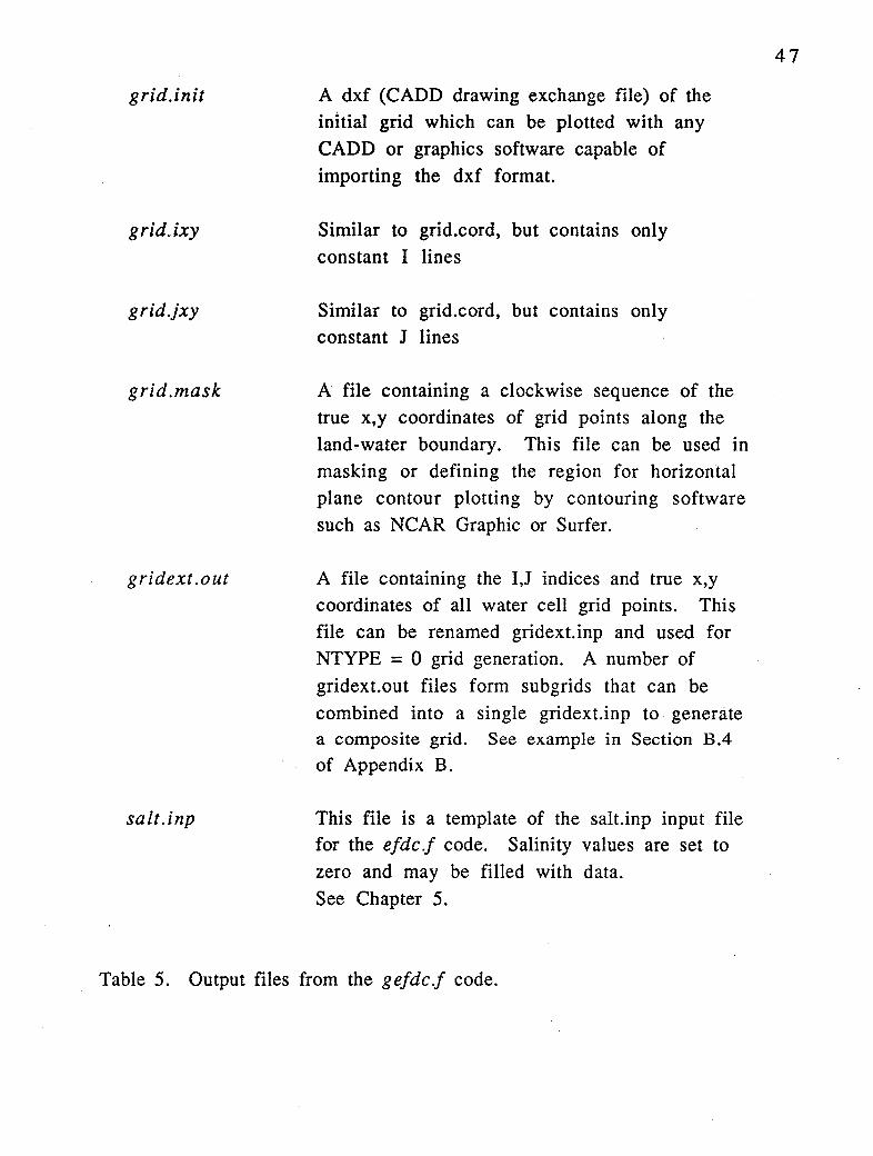
grid.init

grid.ixy

grid.jxy

grid.mask

gridext.out

salt.inp

A dxf (CADD drawing exchange file) of the initial grid which can be plotted with any CADD or graphics software capable of importing the dxf format.

Similar to grid.cord, but contains only constant I lines

Similar to grid.cord, but contains only constant J lines

A file containing a clockwise sequence of the true x,y coordinates of grid points along the land-water boundary. This file can be used in masking or defining the region for horizontal plane contour plotting by contouring software such as NCAR Graphic or Surfer.

A file containing the I,J indices and true x,y coordinates of all water cell grid points. This file can be renamed gridext.inp and used for NTYPE = 0 grid generation. A number of gridext.out files form subgrids that can be combined into a single gridext.inp to. generate a composite grid. See example in Section B.4

of Appendix B.

This file is a template of the salt.inp input file for the efdc .f code. Salinity values are set to zero and may be filled with data. See Chapter 5.

Table 5. Output files from the gefdc.f code.

47

48

I ,J HII HJJ HIIHJJ JACOBIAN ANG ERROR

39 6 0.1968E+02 0.2962E+02 0.5827E+03 0.5827E+03 0.3120E+OO

ASQRTG--= 0. 3305E+06 ASHIHJ= 0. 3311E+06 AERR= 0 .1973E-02 NaI.LS= 325

Figure 9. Sample output in the dxdy.diag file.

DIFF INITIAL X&Y, ITER = 100 RSX,RSY = 0.4439E-10 0.4383E-11

DIFFUSE RKI, ITERATION= 69 RSK = 0.9475E-12

DIFF X & Y, ITER =: 81 RSX,RSY = 0. 9747E-12 0. 8887E-12

GRID GENERATION LCOP ITERATION = 1

GI.DEAL RES SQ DIFF' IN RKI= 0.3978E+OO

MIN AND MAX DEVIA'I'ICN FRCM ORTHO = 0.3837E-02 0.1008E+02

:twa:LLS= 325 N999 = 0 DEP:MAX = 0.30678E+Ol

Figure 10. Sample output in the gefdc.log file.

The file dxdy.diag, Figure 9, contains the primary diagnostics of the curvilinear-orthogonal grid generation process. For each water cell, the file lists the computed orthogonal metric factors HI and HG (which are also dx and dy, the curvilinear cell dimensions). For true orthogonality, the product HII*HJJ is the horizontal area of the cell. The actual area of the cell, which is also the Jacobian of the general curvilinear coordinate transformation, is also shown, and should agree with HII*HJJ to within a few percent. The angular error for each cell is a measure of deviation from numerical orthogonality, and should be small. The orthogonality of the grid can be improved by identifying cells along the land water boundary with the largest angular errors and adjusting their land bounding grid corner coordinate points on Card Image 13 in the g ef de. i np file. At the end of the dxdy.diag file, the exact area of the grid, ASQRTG, is printed for comparison with the sum of the HII*HJJ product for all water cells. The relative error between these two quantities, AERR, is also printed, as well as the total number of water cells in the grid. The gefdc.log file, shown in Figure 10, summarizes the computational steps in the grid generation. The initialization of the grid, referred to as diffuse x and y, since the generation scheme is similar to the solution of a steady state diffusion or elliptic equation, is followed by a summary of each grid generation iteration. The iteration involves diffusing the boundary metric ratios, RKI, to the interior and then the diffusion of the x and y coordinates to the interior. The residuals for these diffusion or elliptic equation solutions by successive over

relaxation are the small quantities beginning with R. The minimum and maximum deviations from orthogonality, in degree, at the end of the iteration is then printed. After the grid generation has converged or executed the specified number of maximum iterations, the equivalent contents of the dxdy. out (inp) file is also written in gefdc.log. The file ends with a summary of the number of water cells, the number of cells where depth or bottom topography failed to be determined, and the maximum initial water depth in the grid.

49

4. The Master Input File

This chapter describes the master input, efdc.inp, for the efdc.f code. The information in efdc.inp provides run control parameters, output control and physical information describing the model domain and external forcing functions. The file is internally documented, in essence providing a template or menu for setting up a simulation. The file consists of card image sections, with each section having header lines which define the relevant input parameter in that section. The function of the various card image sections is best illustrated by a sequential discussion of each section. Card Image sections and input parameters which are judged to be clearly explained in the ef d c. i np files internal documentation will not be discussed specifically. Before proceeding, a number of conventions should be discussed. Many options in the code are activated by integer switches (most beginning with either IS or JS). Unless otherwise noted, setting theses switches to zero deactivates the option. Options are normally activated by specifying nonzero integer values. A number of options described in the file are classified as for research purposes. This classification indicates that the option may involve an experimental and not fully tested numerical scheme or that it involves rather complex internal analysis or flow field data extraction. Detail information on the function and current status of these options may be obtained from the writer. A complete listing of the efdc.inp file for an actual application can be found in Appendix C,

and may be used as the template for setting up a new model application.

50

Card Image 1

Cl TITIE FOR RUN C

TITIE OR IDENI'IFIER FOR THIS INPUT FIIB AND RUN C Cl (LIMIT TO 80 OJARACTERS LENGTH)

'JAMES RIVER 6 LAYERS, FINAL CALIBRATION RUN'

Card Image 2

C2 RESTART, GENERAL CONTROL AND DIAGNOSTIC SWITCHES C

C

ISRESTI: 1 FOR READING INITIAL CONDITIONS FRCM FILE restart.inp

-1 AS ABOVE BUT ADJUST FOR CHANGING BOTTCM ELEVATICN 2 INITIALIZES A KC IAYER RUN FRCM A KC/2 IAYER RUN

FOR KC.GE.4 10 FOR READING !C'S FRCM restart.inp WRITTEN BEFORE 8

SEPT 1992 ISREST0:-1 FOR WRITING RESTART FIIB restart.out AT END OF RUN

N INTE.GER.GE.0 FOR WRITING restart.out EVERY N REF TIME PERICDS

ISRESTR: 1 FOR WRITING RESIDUAL TRANSPORT FILE restran.out ISP.AR: 0 FOR EXECUTION OF CODE ON A SINGLE PROCESSOR MACHINE

1 FOR PARALLEL EXE, PARAI.J.ELIZING PRIMARILY OVER IAYERS 2 FOR PARALLEL EXE, PARALLELIZING PRIMARILY OVER

NIM HORIZONTAL GRID SUBDOMAINS, SEE CARD C9 ISICG: 1 FOR WRITING 1CG TO SCREEN AND FILE efdc.log

2 FOR WRITJN; TO FIIB efdc.log ONLY ISDIVEX: 1 FOR WRITING EXTERNAL MODE DIVERGENCE TO SCREEN ISNEGH: 1 FOR SEAROIING FOR NEGATIVE DEPTHS AND WRITING TO

SCREEN ISMM::: 1 FOR WRITING MIN AND MAX VALUES OF SALT AND DYE

CONCENTRATICN TO SCREEN ISBAL: 1 FOR ACTIVATING MASS, MOMENTUM AND ENERGY BALANCES

AND WRITING RESULTS TO FILE bal.out ISHP: 1 FOR CALLING HP 9000 S700 VERSIONS OF CERTAIN

SUBROUTINES !SHOW: 1 TO SHOW PW&S ON SCREEN, SEE INSTROCTIONS FOR FILE

show.inp

5 1

C2 ISRESTI ISRESTO ISRESTR ISP.AR IS1CG ISDIVEX ISNEGH ISMM:: ISBAL ISHP !SHOW 1 4 0 0 2 0 0 0 0 0 0

Card Image 2, specifies the mode of model startup, either a cold start, with the flow field initialized to zero, or a restart.inp using initial

conditions corresponding to the conditions at the end of a previous simulation. The ISRESTO switch controls the frequency of outputting restart information to the file restart.out (which is renamed restart.inp to launch a run). The file restran.out contains the time averaged transport file, which may be used to execute the ef dc.f code in a transport only mode. The switch ISPAR allows implementation of internal code options for execution on multiple processor or parallel machines. These options are currently supported on multiple vector processor Cray supercomputers, and on Silicon Graphic and Spare (Sun and clones) based symmetric multiprocessor UNIX workstations. The choice of ISP AR equal to 1 or 2, depends on both the grid structure and the number of processors on which the code will execute. Portions of the code capable of being parallelized over vertical layers or horizontal grid subdomains are parallelized over vertical layers when ISP AR is set to 1. For layer parallelization, the number of layers must be an integer multiple of the number of processors on which the code will execute. For grids consistent with layer parallelization, portions of the code allowing either mode of parallelization are generally more efficient 1n the layer parallelization mode. Certain portions of the code may be parallelized only overly horizontal subdomains, with this mode being active for ISP AR equal 1 or 2. For ISP AR = 2, all parallelization is over horizontal subdomains. See Card C9 and chapter 6 for additional details regarding parallel execution of EFDC. The switch ISLOG activates the creation of a log file (ISLOG = 2, recommended)

which is deleted and reopened after each reference time period. The contents and interpretation of the material in file efdc.log will be discussed in . the diagnostics chapter. The switches, ISDIVEX, ISNEGH, and ISMMC, activate diagnostic checks on volume conservation, identify negative solution depths, and check mass conservation of transport materials, activation of these switches (IS=l) produces identical output to the screen and efdc.log file. The use of these options for diagnostic purposes is discussed in the diagnostics chapter. The switch ISHP allows use of Hewlett-Packard 9000 series 700 vector libraries. The vector library calls are currently commented out with CDHP in the source code. The procedure for

52

activating this option and accessing the HP vector library may be obtained from the writer. The switch ISBAL activates an internal volume, mass, momentum and energy balance procedure. The switch ISHOW activates a screen print of flow field conditions in a specified horizontal location during the run, with more details given with the description of the file show .inp in the next chapter.

Card Image 3

C3 EXTERNAL M:>DE SOimION OPTION PARAMETERS AND SWITCHES C

C

RP: RS~: !TERM: IRVEC:

RP.ADJ:

RSCMADJ:

ITRMADJ:

ITERHPM:

IDRYCK:

ISDSOLV:

OVER RELAXATICN PARAMETER TARGET SQUARE RESIDUAL OF ITERATIVE SOimION SCHEME MAXIMUN NUMBER OF ITERATICNS

0 STANDARD RED-BIACK SOR SOimION 1 MJRE VECTORIZABLE RED-BLACK SOR

(FOR RESEAROI PURPOSES) 2 RED-BLACK ORDERED CONJUGATE GRADIENT SOLUTICN 3 REDUCED SYSTEM R-B CONJUGATE GRADIENT SOLUTICN

RELAXATION PARAMETER FOR AUXILIARY POTENTIAL ADJUSTMENT OF THE MEAN MASS TRANSPORT ADVECTICN FIEID (FOR RESEARCH PURPOSES) TARGET SQUARED RESIDUAL ERROR FOR ADJUSTMENT (FOR RESEAROI PURPOSES)

MAXIMUM ITERARTIONS FOR ADJUSTMENT (FOR RESEARQI PURPOSES)

MAXIM.M ITERATIONS FOR STRONGLY NONLINEAR DRYING AND WETTING SCHEME (ISDRY=3 OR OR 4) ITERHPM.LE.4 ITERATIONS _PER DRYING CHECK (ISDRY .GE.1) 2.LE.IDRYCK.LE.20

1 TO WRITE DIAGNOSTICS FILES FOR EXTERNAL MODE SOLVER

C3 RP RS~ ITERM IRVEC RP.ADJ RSCMADJ ITRMADJ ITERHPM IDRYCK ISDSOLV 1.8 1.E-8 100 3 1.8 l.E-16 1000 0 20 0

The information input on Card Image 4 primarily controls the external or barotropic mode solution in efdc .f. The relaxation parameter of 1.8 should not be changed. The RSQM parameter is the residual squared error in the external mode solution. It is generally set between lE-6 and lE-15, with the small values corresponding several hundred cells and a small time step (10-100 seconds) and the larger value corresponding a large number of cells (1000-10,000) and a large time~ step (100-1000 seconds). It RSQM is set to a small

53

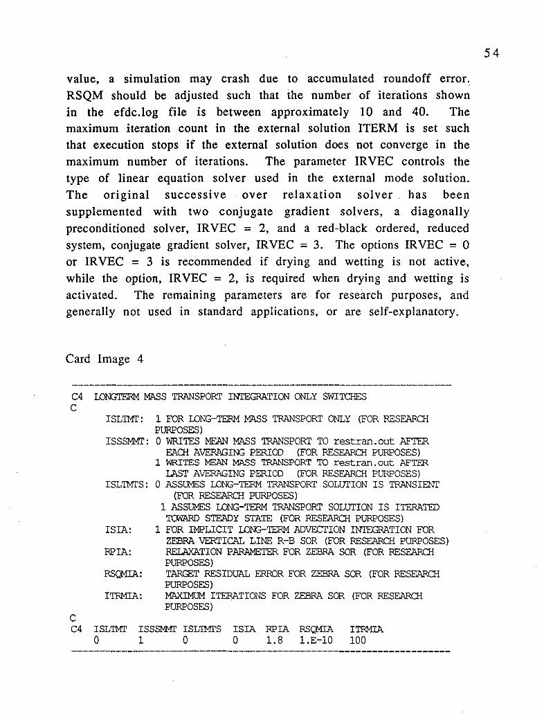
value, a simulation may crash due to accumulated roundoff error. RSQM should be adjusted such that the number of iterations shown in the efdc.log file is between approximately 10 and 40. The maximum iteration count in the external solution ITERM is set such that execution stops if the external solution does not converge in the maximum number of iterations. The parameter IRVEC controls the type of linear equation solver used in the external mode solution. The original successive over relaxation solver has been supplemented with two conjugate gradient solvers, a diagonally preconditioned solver, IRVEC = 2, and a red-black ordered, reduced system, conjugate gradient solver, IRVEC = 3. The options IRVEC = 0 or IRVEC = 3 is recommended if drying and wetting is not active, while the option, IRVEC = 2, is required when drying and wetting is activated. The remaining parameters are for research purposes, and generally not used in standard applications, or are self-explanatory.

Card Image 4

C4 LONGTERM MASS TRANSPORT INTEGRATION ONLY SWITCHES C

C

ISL'IMI': 1 FOR LONG-TERM MASS TRANSPORT ONLY (FOR RESEARCH PURPOSES)

ISSSMMT: 0 WRITES MEAN MASS TRANSPORT TO restran.out AFTER EACH AVERAGING PERIOD (FOR RESEARCH PURPOSES)

1 WRI'IES MEAN MASS TRANSPORT TO restran.out AFTER LAST AVERAGING PERIOD (FOR RESEARCH PURPOSES)

ISL'IMI'S: 0 ASSUMES LONG-TERM TRANSPORT SOLUTION IS TRANSIENT (FOR RESEARCH PURPOSES)

1 ASSUMES LONG-TERM TRANSPORT SOLUTION IS ITERATED TCWARD STEADY STATE (FOR RESEARCH PURPOSES)

ISIA: 1 FOR IMPLICIT LONG-TERM ADVECTION INTEGRATION FOR ZEBRA VERTICAL LINE R-B SOR (FOR RESEARCH PURPOSES)

RPIA: RELAXATION PARAMETER FOR ZEBRA SOR (FOR RESEARCH PURPOSES)

RSQMIA: TARGET RESIDUAL ERROR FOR ZEBRA SOR (FOR RESEARCH PURPOSES)

ITRMIA: MAXIMUM ITEM,TIONS FOR ZEBRA SOR (FOR RESEARCH PURPOSES)

C4 ISLTMI' ISSSMMI' ISLTMI'S ISIA RPIA RSQMIA ITRMIA 0 1 0 0 1.8 l.E-10 100

54

The EFDC model has the capability to function in a transport only mode using advective and diffusive transport specified in the file restran.inp. The first parameter, ISLTMT, actives this mode. The second parameter ISSSMMT controls the creation of the restran.inp file, output as restran.out, during normal execution. The frequency of graphical output of residual fields is also controlled by this parameter. The third parameter determines whether the transport only mode with be integrated to steady state or integrated for a transient residual transport field. The remaining four parameters are for research purposes, however, ISIA should be set to zero.

55

56

Card Image 5

CS Ml1ENTUM NJVI!I:. AND HORIZ DIFF SWITQIBS AND MISC SWITQIBS C

ISCDMA:

ISAHMF:

ISWASP: ISDRY:

s

ISQQ: ISRLID: ISVEG:

ISVEGL:

ISITB:

ISWAVE

C

1 FOR CENTRAL DIFFERENCE M:lMENTUM ADVECTION 0 FOR UPWIND DIFFERENCE ~ ADVECTION 2 FOR EXPERIMENTAL UPWIND DIFF M:t-1 ADV

(FOR RESEARCli PURPOSES) 1 TO ACTIVATE HORIZONTAL M:lMENTUM DIFFUSION

ISDISP: 1 CALCULATE MEAN HORIZONTAL SHEAR DISPERSION TENSOR OVER LAST MEAN MASS TRANSPORT AVERAGING PERIOD

4 or 5 TO WRITE FIIES FOR WASP4 or WASPS MODEL LINKAGE GREATER THAN O TO ACTIVE WETTING & DRYING OF HALI.OW AREAS

1 CONSTANT WETTING DEPTH SPECIFIED BY HWET ON CARD 11 WITH NONLINEAR ITERATIONS SPECIFIED BY ITERHPM ON CARD C3

2 VARIABLE WETTING DEPTH CALCULATED INTERNALLY IN CCOE WITH NONLINEAR ITERATIONS SPECIFIED BY ITERHPM ON CARD C3

11 SAME AS 1, WITHOUT NONLINEAR ITERATION 12 SAME AS 2, WITHOUT NONLINEAR ITERATION

3 DIFFUSION WAVE APPROX, CONST.ANT WETTING DEPTH (NOT ACTIVE)

4 DIFFUSION WAVE APPROX, VARIABIE WETTING DEPTH (NOT ACTIVE)

1 1:0 USE STANDARD TURBULENT INTENSITY ADVECTION SCHEME 1 1:'() RUN IN RIGID LID MODE (NO FREE SURFACE) 1 TO IMPLEMENT VEGETATION RESISTAN:E 2 IMPLEMENT WITH DIAGNOSTICS TO FIIE cbot.log 1 TO INCLUDE LAMINAR F1DW OPTION IN VEGETATION

RESISTAN:E 1 FOR IMPLICIT BO'ITCM & VEGETATION RESISTANCE·IN

EXTERNAL M)I)E FOR SINGLE LAYER APPLICATIONS (KC=l) 1 FOR WAVE CURRENT BOUNDARY LAYER 2 FOR W::: BL AND WAVE INDUCED CURRENTS

BOTH OPTIONS REQUIRE FIIE wave.inp

CS ISCDMA. ISAHMF ISDISP ISWASP ISDRY ISQQ ISRLID ISVEG ISVEGL ISITB ISWAVE 0 0 0 0 0 1 0 0 0 0 0

This card image controls various options for integration of the advective and diffusive portions of the momentum equations as well as the activation of additional physical process representations and optional output processing. The parameter ISCDMA controls the finite difference representation of momentum advection, with the

zero default value corresponding to upwind difference, and the values of 1 and 2 corresponding respectively to central differencing and an experimental upwind difference scheme. The central difference option is generally recommended only for smooth or idealized bottom topography and lateral boundaries. The second parameter ISAHMF activates horizontal moment diffusion. It should be activated when using central difference advection or when simulating wave induced currents. For wave induced currents, the horizontal diffusion is specified in terms of the wave energy dissipation due to wave breaking in the surf zone. The options ISDISP and ISWASP respectively control the creation of shear dispersion coefficient file <lisp.out and a WASP water quality model transport files waspX.out. The parameter ISDRY activates drying and wetting and the value 11 is recommended. The parameter ISQQ should remain set to unity. The parameter ISRLID implements a rigid free surface simulation and is generally used only for research purposes. The next three parameters activate the vegetation resistance model. The last parameter ISITB should be activated only in single layer or depth integrated simulations. The remaining parameter ISW A VE activates the wave-current boundary layer model and the wave induced current model, using an external specification of high frequency surface wave conditions in the input file wave.inp.

57

Card Image 6

C6 DISSOLVED AND SUSPENDED CONSTITUENT TRANSPORT SWITCHES C6 TURB INT=O, SALT=l, TEMP=2, DYEC=3, SEDC=4, SFL=S, CWQ=6 C

ISTRAN: ISTOPT: ISCIXA:

ISADAC:

ISFCT:

ISPLIT:

ISADAH:

ISADAV:

!SCI: ISCO:

C

1 TO ACTIVATE TRANSPORT CONSTITUENT SPECIFIC TRANSPORT OPTICNS

0 FOR STANDARD DONOR CELL UPWIND DIFFERENCE ADVECTION 1 FOR CENTRAL DIFFERENCE ADVECTION FOR THREE TIME

lEVEL STEPS 2 FOR EXPERIMENTAL UPWIND DIFFERENCE ADVECTION (FOR

RESEAROI PURPOSES) 1 TO ACTIVATE ANTI-NUMERICAL DIFFUSICN CORRECTION TO

STANDARD DONOR CELL SCHEME 1 TO ADD FLUX LIMITIN:; TO ANTI-NUMERICAL DIFFUSICN

CORRECTION 1 TO OPERATOR SPLIT HORIZONTAL AND VERTICAL ADVECTION

(FOR RESEARQI PURPOSES) 1 TO ACTIVATE ANTI-NUM DIFFUSION CORRECTION TO

HORIZONTAL SPLIT ADVECTION STANDARD DONOR CELL SCHEME (FOR RESEARCH PURPOSES)

1 TO ACTIVATE ANTI-NUM DIFFUSION CORRECTION TO VERTICAL (FOR RESEARCH PURPOSES) SPLIT ADVECTION STANDARD DONOR CELL SCHEME (FOR RESEARQI PURPOSES)

1 TO READ CONCENTRATION FRCM FILE restart.inp 1 TO WRITE CONCENTRATION TO FILE restart.out

C6 ISTRAN ISTOPT ISCDCA ISADAC ISFCT !SPLIT ISADAH ISADAV ISCI ISCO 1 0 0 0 0 0 0 0 0 0 !turb 1 0 0 1 1 0 0 0 1 1 !salt 1 0 0 1 1 0 0 0 1 1 !temp 0 0 0 1 1 0 0 0 0 0 !dye 0 0 0 1 1 0 0 0 0 0 !sed O O O 1 1 O O O O O !tsfl 0 0 0 1 1 0 0 0 0 0 !cwq

Card Image 6 controls the advective transport and source sink options for transported scalar fields. The seven lines of active input represent in order, turbulent intensity, salinity, temperature, a dye tracer, suspended sediment, shellfish larvae, and water quality variables. The 'first switch, ISTRAN activates advective transport and sources and sinks. On the first line, corresponding to the turbulence model, only ISTRAN should be set to unity with the remaining parameters set to zero. For water quality, ISTRAN=l, activates the

58

embedded water quality model WQ3D (Park, 1995) which has additional input files not documented in this manual. The second parameter ISTOPT sets options for a number of the transport scalar fields. Current active options are:

Salinity ISTOPT=l: Read initial salinity distribution from file

salt.inp (ISRESTl=O, only)

Temperature ISTOPT=l: Full surface and internal heat transfer

calculation using data from file aser.inp. ISTOPT=2: Transient equililibrium surface heat transfer

calculation using external equilibrium temperature and heat transfer coefficient data from file aser.inp.

ISTOPT=3: Equilibrium surface heat transfer calculation using constant equilibrium

temperature and heat transfer coefficients from Card Image 30.

Initial isothermal temperature for cold starts (ISRESTI=O) is read on Card Image 30. See Cereo and Cole (1993) for a discussion of the equilibrium temperature surface · head transfer approach.

Dye Tracer ISTOPT=l: Read initial dye tracer distribution from file

dye.inp (ISRESTI=O, only). Linear or first order dye decay specified on Card Image 30.

Suspended Sediment ISTOPT~l: Suspended sediment is cohesive. Settling,

deposition and resuspension calculated in subroutine CALSED

ISTOPT=2: Suspended sediment is cohesive. Settling,

59

deposition and resuspension calculated in subroutine CALSED2

ISTOPT=3: Suspended sediment is noncohesive. Settling, deposition and resuspension calculated in subroutine CALSED3

ISTOPT=4: Suspended sediment is noncohesive. Settling, deposition and resuspension calculated in subroutine CALSED3 after wave wave-current boundary layer or wave induced forcing have been gradually introduced.

Sediment settling, resuspension, and deposition data is read on CARD Image 29.

Shellfish Larvae No options available

Water Quality Constituents ISTOPT=l: Specifies 20 water column state variables. ISTOPT=2: Specifies 14 water column state variables. ISTOPT=3: Specifies 8 water column state variables.

The third parameter, ISCDCA, specifies the advection scheme with the zero default values corresponding to donor cell upwind difference. Values of 1 and 2 specify central difference (not recommended) and an experimental first order upwind difference scheme, respectively. The parameter ISADAC=l activates an antidiffusion advective flux correction (Smolarkiewicz and Clark, 1986) for ISCDCA equals O or 1. The parameter ISFCT=l, implements the antidiffusion correction in the flux corrected transport form (Smolarkiewicz and Grabowski, 1990). The three parameters ISPLIT, ISADAH, and ISADA V activate an experimentally operated split antidiffusive upwind difference scheme and should remain set to 0. The parameters ISCI and ISCO when set to 1 read and write, respectively, the specified field from and to the files restart.inp and

restart.out. Turbulence quantities are by default read from and written to the restart files.

60

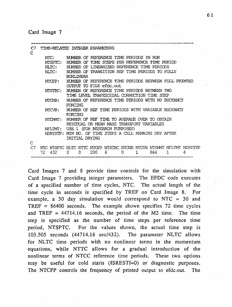
Card Image 7

C7 TIME-REI.ATED INTE',GE:R PARAMETERS C

NTC: NTSPTC: NLTC: NLTC:

Nl'CPP:

NTSTBC:

NI'CNB:

NTCVB:

NTCM1T:

NFL'IMI': NDRYSTP:

C

NtMBER OF REFERENCE TIME PERIODS IN RUN NUMBER OF TIME STEPS PER REFERENCE TIME PERICO NUMBER OF LINEARIZED REFERENCE TIME PERIODS NUMBER OF TRANSITION REF TIME PERIODS TO FULLY NONLINEAR NUMBER OF REFERENCE TIME PERIODS BETWEEN FULL PRINTED OUTPU'I' TO FIIE efdc. out NUMBER OF REFERENCE TIME PER.IC.OS BETWEEN TW)

TIME: IEVEL TRAPEZOIDAL CORRECTION TIME STEP NUMBER OF REFERENCE TIME PERIODS WITH NO BUOYANCY FORCING NUMBER OF REF TIME PERIODS WITH VARIABLE BUOYANCY FORCING NUMBER OF REF TIME TO AVERAGE OVER TO OBTAIN RESIDUAL OR MEAN MASS TRANSPORT VARIABLES USE 1 (FOR RESEARCH PURPOSES) MIN NO. OF TIME STEPS A CELL REMAINS DRY AFTER INI'rIAL DRYING

C7 NTC NTSPTC NLTC NTTC NTCPP NTSTBC NTCNB NTCVB NTSM1I' NFL'IMI' NDRYSTP 72 432 0 0 200 6 0 1 864 1 4

Card Images 7 and 8 provide time controls for the simulation with Card Image 7 providing integer parameters. The EFDC code executes of a specified number of time cycles, NTC. The actual length of the time cycle in seconds is specified by TREF on Card Image 8. For example, a 30 day simulation would correspond to NTC = 30 and TREF = 86400 seconds. The example shown specifies 72 time cycles and TREF = 44714.16 seconds, the period of the M2 time. The time step is specified as the\ number of time steps per reference time period, NTSPTC. For the values shown, the actual time step is 103.505 seconds (44714.16 sec/432). The parameter NLTC allows for NL TC time periods with no nonlinear terms in the momentum equations, while NTTC allows for a gradual introduction of the nonlinear terms of NTCC reference time periods. These two options may be useful for cold starts (ISRESTI=O) or diagnostic purposes. The NTCPP controls the frequency of printed output to efdc.out. The

61

printed output is primarily in the form of line printer contour plots which may be useful in situations where graphics postprocessing capabilities are not readily available. Given the extensive options currently available in the code to generate graphical output, NTCPP is usually specified large enough such that the printed output is not generated. The parameter, NTSTBC is extremely important in that it specifies the frequency of insertion of a two time level trapezoidal correction step into the three-time level integration (see Hamrick, 1992a). Generally NTSTBC should be between 4 and 12, increasing if

NTSPTC increases. The parameters NTCNB and NTCVB control the introduction of buoyancy forcing into the momentum equations in a similar manner as described for NL TC and NTTC. The parameter NTSMMT specifies the number of time steps for the calculation of time averaged or residual output variables and also the output frequency to the "r" class output files. If NTSMMT is greater than or equal to NTSPTC, the averaging includes calculation of the Lagrangian mean transport fields (Hamrick, 1994a). The parameter NFL TMT should remain set to 1. The parameter NDRYSTP specifies the number of timesteps a cell must remain dry before wetting is allowed when the drying and_ wetting option is activated.

62

Card Image 8

ca TIME-REI.ATED REAL PARAMETERS C

'ICON: TBEGIN: TREF:

CORIOLIS: ISCCA:

ISCFL:

C

CONVERSION MULTIPLIER TO CHANGE TBEGIN TO SECONDS TIME ORIGIN OF RUN REE'EREN:E TIME PERIOD IN SEC (i.e. 44714.16s or 86400s)

CONSTANT CORIOLIS PARAMETER IN 1/SEC WRITE DIAGNOSTICS FOR MAX CORIOLIS--OJRV ACCEL TO FILE efdc.log WRITE DIAGNOSTICS OF MAX THEORETICAL TIME STEP TO FIIE cfl.out

C8 'ICON TBEGIN TREF CORIOLIS ISOCCA ISCFL 3600. 3173.7166 44714.16 0.0001 0 0

This card image specifies a number of real time related parameters as well as activating timestep related diagnostics. TBEGIN specifies the start time of the runs in units of seconds, minutes, hours, or days, with TCON being the multiplier factor which would convert TBEGIN to seconds. The reference time period must always be specified in seconds. The EFDC model currently is based on an f plane formulation for the Coriolis accelerations, with the variable CORIOLIS being the value of f in 1/seconds units. The maximum stable time

step is constrained by the 0.5/f and the CFL criteria for advection (Hamrick, 1992a). Activation of ISDCCA causes the maximum effective Coriolis parameter to be printed to the log file efdc.log at each time step. Activation of ISCFL=l writes the limiting time step, and the cell in which it occurs, based on the CFL condition to the file cfl out at each time step. Since the CFL condition is based on linear stability analysis of a constant coefficient, three-dimensional advection equation, a good rule for real world applications with spatial and temporal varying advective fields is to use a time step on the order of 1/4 to 1/2 the limiting CFL time step written to cfl.out. Since both of the time step diagnostics involve logic searches, they

should only be activated during the start up of a new model application.

63

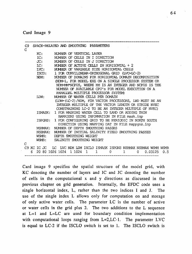
Card Image 9

C9 SPACE-REIATED AND SMX>THJN3 PARAMETERS C

KC: IC: JC: I.C: LVC: ISCO: NDM:

IDW:

ISMASK:

ISPGNS:

NSHMAX: NSBMAX: WSMH: WSMB:

C

NUMBER OF VERTICAL LAYER NUMBER OF CELLS IN I DIRECTION NUMBER OF CELLS IN J DIRECTION NU1BER OF ACTIVE CELLS IN HORIZONTAL + 2 NU1BER OF VARIABLE SIZE HORIZONTAL CELLS 1 FOR CURVILINEAR-ORTHCX30NAL GRID (LVC=I.C-2) NUMBER OF DCMAINS FOR HORIZONTAL DOMAIN DECCMPOSITION (NDM=l, FOR M)DEL EXE ON A SINGLE PR<XESSOR SYSTEM OR NDM=M.f*NCPUS, WHERE MM IS AN INTEGER AND NCPUS IS THE NUMBER OF AVAILABLE CPU's FOR MODEL EXECUTION ON A PARALLEL MULTIPLE PR<XESSOR SYSTEM)

NUMBER OF WATER CELLS PER DOMAIN {LOW= {LC-2) /NDM, FOR VECTOR PR<XESSORS, LWD MUST BE AN INTEGER MULTIPLE OF THE VECTOR LENGTH OR STRIDE NVEC CONSTRAINING I.C-2 TO BE AN INTEGER MULTIPLE OF NVEC)

1 FOR MASKING WATER CELL TO LAND OR ADDING THIN BARRIERS USING INFORMATION IN FILE mask.inp

1 FOR CONFIGURING GRID TO BE PERIODIC IN NORTH SOUTH DIRECTION USING MAPPING DAT IN FILE mappgns.inp

NUMBER OF DEPTH SMOOTHING PASSES NUMBER OF INITIAL SALINITY FIEID SM:X>THING PASSES DEPTH SMOOTHING WEIGHT SALJNITY SMOOTHING WEIGHT

C9 KC IC JC I.C LVC Ml1 IDM ISCLO ISMASK ISPGNS NSHMAX NSBMAX WSMH WSMB 6 20 80 1026 1024 11024 1 1 0 1 0 0.03125 0.5

Card image 9 specifies the spatial structure of the model grid, with KC denoting the number of layers and IC and JC denoting the number of cells in the computational x and y directions as discussed in the previous chapter on grid generation. Internally, the EFDC code uses a single horizontal index, L, rather than the two indices I and J. The use of the single index L allows only for computation on and storage of only active water cells. The parameter LC is the number of active or water cells in the grid plus 2. The two additions to the L sequence at L=l and L=LC are used for boundary condition implementation with computational loops ranging from L=2,LC-1. The parameter L VC is equal to LC-2 if the ISCLO switch is set to 1. The ISCLO switch is

64

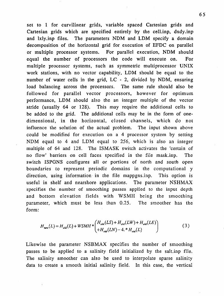
set to 1 for curvilinear grids, variable spaced Cartesian grids and Cartesian grids which are specified entirely by the cell.inp, dxdy .inp and lxly.inp files. The parameters NDM and LDM specify a domain decomposition of the horizontal grid for execution of EFDC on parallel or multiple processor systems. For parallel execution, NDM should equal the number of processors the code will execute on. For multiple processor systems, such as symmetric multiprocessor UNIX work stations, with no vector capability, LDM should be equal to the number of water cells in the grid, LC - 2, divided by NDM, ensuring load balancing across the processors. The same rule should also be followed for parallel vector processors, however for optimum performance, LDM should also the an integer multiple of the vector stride (usually 64 or 128). This may require the additional cells to be added to the grid. The additional cells may be in the form of onedimensional, in the horizontal, closed channels, which do not influence the solution of the actual problem. The input shown above could be modified for execution on a 4 processor system by setting NDM equal to 4 and LDM equal to 256, which is also an integer multiple of 64 and 128. The ISMASK switch activates the 'certain of no flow' barriers on cell faces specified in the file mask.inp. The switch ISPGNS configures all or portions of north and south open boundaries to represent periodic domains in the computational y direction, using information in the file mappgns.inp. This option is useful in shelf and nearshore applications. The parameter NSHMAX specifies the number of smoothing passes applied to the input depth

and bottom elevation fields with WSMH being the smoothing parameter, which must be less than 0.25. The smoother has the form:

Htvt}L)=Ho,AL)+WSMH* old old old (

H (LS)+ H (LW) + H (LE)J

+Hold(LN)-4. * Hold(L) (3)

Likewise the parameter NSBMAX specifies the number of smoothing passes to be applied to a salinity field initialized by the salt.inp file. The salinity smoother can also be used to interpolate sparse salinity data to create a smooth initial salinity field. In this case, the vertical

65

salinity profiles in the salt.inp file must be set with zero values, except at locations where nonzero values are supplied. Setting NSBMAX to a large number, which must be greater than 10, and should usually be on the order of 2000, interpolates the salinity over the entire grid with the nonzero input data unmodified. In an estuary application, specifying small values at the limit of salinity intrusion will prevent the diffusive interpolation scheme from progressing upstream.

66

Card Image 10

ClO !AYER THICKNESS IN VERTICAL C

C

THICKNESS OF EACH VERTICAL IAYER, 1 = BOTl'CM !AYER THICKNE:SSES MUST SUM TO 1. 0

ClO !AYER NUMBER 1

DIMENSICNLESS IAYER THICKNESSES 0.166

2 0.167 3 0.167 4 0.167 5 0.167 6 0.166

Card Image 10 (older versions)

ClO IAYER THICKNESS IN VERTICAL C

C

THICKNESS OF EACH VERTICAL lAYER, 1 = BOTT01 IAYER THICKNESSES MUST SUM TO 1.0

ClO 1 2 3 4 5 6 7 8 0.166 0.167 0.167 0.167 0.167 0.166

This card specifies the dimensional thickness of the vertical layers,

which do not have to be equal.

67

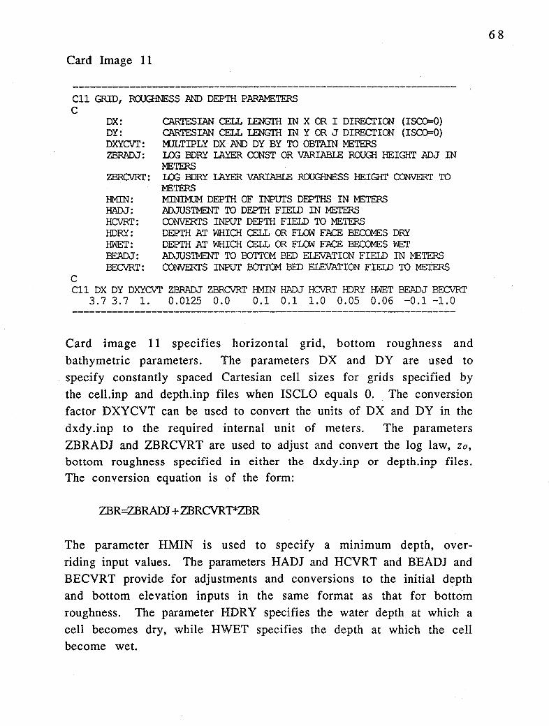
Card Image 11

Cll GRID, ROOGHNESS AND DEPTH PARAMETERS C

DX: DY: DXYCVT: ZBRADJ:

ZBRCVRT:

HMIN: HADJ: HCVRT: HDRY: HWET: BE.ADJ: BECVRT:

C

CARTESIAN CELL LENGTH IN XOR I DIRECTION (ISCO=O) CARTESIAN CELL LENGTH IN Y OR J DIRECTION (ISCO=O) MJLTIPLY DX AND DY BY TO OBTAIN METERS I..03 BDRY IAYER CONST OR VARIABIE ROUGH HEIGHT ADJ IN METERS I..03 BDRY IAYER VARIAB1E ROUGHNESS HEIGHT CONVERT TO ME~t'ERS MINIMUM DEPTH OF INPUTS DEPTHS IN METERS ADJUSTMENT TO DEPTH FIEID IN METERS CONVER1~S INPUT DEPTH FIEID TO METERS DEPTH AT MUOI CELL OR FLOW FACE BECCMES DRY DEPTH AT WHIOI CELL OR FLOW FACE BECCMES WET ADJUSTMENT TO BOTTOM BED ELEVATION FIEID IN METERS CONVERTS INPUT BOTTOM BED ELEVATION FIEID TO METERS

Cll DX DY DXYCVT ZBRAD~r ZBRCVRT HMIN HADJ HCVRT HDRY HWET BEADJ BECVRT 3.7 3.7 1. 0.0125 0.0 0.1 0.1 1.0 0.05 0.06 -0.1 -1.0

Card image 11 specifies horizontal grid, bottom roughness and bathymetric parameters. The parameters DX and DY are used to specify constantly spaced Cartesian cell sizes for grids specified by the cell.inp and depth.inp files when ISCLO equals 0. The conversion factor DXYCVT can be used to convert the units of DX and DY in the dxdy .inp to the required internal unit of meters. The parameters ZBRADJ and ZBRCVRT are used to adjust and convert the log law, zo, bottom roughness specified in either the dxdy .inp or depth.inp files.

The conversion equation is of the form:

ZBR=ZBRADJ + ZBRCVRT*ZBR

The parameter HMIN is used to specify a minimum depth, overriding input values. The parameters HADJ and HCVRT and BEADJ and BE CVR T provide for adjustments and conversions to the initial depth and bottom elevation inputs in the same format as that for bouo·m roughness. The parameter HDRY specifies the water depth at which a cell becomes dry, while HWET specifies the depth at which the cell become wet.

68

Card Image 12

C12 TURBUIENT DIFFUSION PARAMETERS C

AHO: AHO: AVO: ABO: AVBCON:

ISFAVB: C C12 AHO AHO

0.0 0.0

CONSTANT HORIZONTAL M:l1ENI'UM AND MASS DIFFUSIVITY M*M/S DIMENSIONLESS HORIZONTAL M:l1ENI'UM DIFFUSIVITY M)LECULAR KINEMATIC VISCOSITY M*WS M)LECULAR DIFFUSIVITY M*WS EQUAI.S ZERO FOR CONSTANT VERTICAL VISCOSITY AND DIFFUSIVITY EQUAL TO AVO AND ABO SET TO 1 TO SQRT FILTER AW AND AVB

AVO 1.E-6

ABO 1.E-9

AVBCON ISFAVB 1.0 0

Card image 12 provides information for horizontal and vertical momentum and mass diffusion. A spatially constant horizontal diffusion is specified by a constant value AHO. A variable horizontal diffusion may be added to the constant value by specifying a nonzero value of ARD, which is the dimensionless constant in the Smagorinsky subgrid scale horizontal diffusion formulation (Smagorinsky, 1963). The background molecular kinematic viscosity and diffusivity are specified by A VO and ABO respectively. When A VBCON is set to 0, the turbulence model is deactivated and the vertical viscosity and diffusivity are set to A VO and ABO respectively. Using this option and setting A VO and ABO to larger values representing turbulent flow readily allows model results to be

compared with constant viscosity and diffusivity analytical solutions for vertical current structure. Setting the parameter ISFA VB to 1 activates a square root smoother for both the vertical turbulent viscosity and diffusivity of the form:

AVO(n+l)=SQRT( AVO(n+l)*AVO(n))

where n indicates the timestep. The smoother is particularly useful for flows having strong surface wind stress forcings.

69

Card Image 13

Cl3 TURBULENCE CI.DSURE PARAMETERS C

VKC: CI'URB: CTEl: CTE2: CIE3: CXMIN: CQI.MIN: DMI.MIN:

C

VON KARMAN CONSTANT TURBULEN'l' CONSTANT (UNIVERSAL) TURBULENT CONSTANT (UNIVERSAL) TURBULENT CONSTANT (UNIVERSAL) TURBULENT CONSTANT (UNIVERSAL) MINIMJM TURBULEN'l' INTENSITY SQUARED MINIMUM 'l'URBULENT INTENSITY SQUARED TIME MACRO-SCAIE MINIMJM DIMENSIONLESS MACRO-SCAIE

Cl3 VKC C1'URB CIEl CTE2 CIE3 CXMIN CQI.MIN DMIMrn 0.4 16.0 1.8 1.33 0.53 l.E-8 l.E-16 l.E-8

The turbulence closure parameters should not be modified without consulting the writer!

Card Image 14

C14 PERIODIC FORCING CONSTITUENT AND HARMONIC ANALYSIS PARAMETERS C

MTIDE: ISLSHA: MLLSHA: NI'CLSHA: ISLSTR: ISHTA:

C

NUMBER OF PERIOD FORCING CONSTITUENTS 1 FOR IN PLACE IEAST SQUARES HARMONIC ANALYSIS NUMBER OF LOCATICNS FOR LSHA LENGTH OF LSHA IN INTEGER NUMBER OF REF TIME PERIODS 1 FOR TREND REMOVAL 1 FOR SINGLE TREF PERIOD SURFACE ELEV ANALYSIS

C14 Ml'IDE ISLSHA MLLSHA NTCLSHA ISLSTR ISfITA 7 1 8 56 0 0

Card image 14 provides basic data for specifying periodic water surface elevation f orcings on open boundaries as well as controlling inplace least squares harmonic analysis of modeling predictions. MTIDE specifies the number of periodic constituents. ISLSHA activates the least squares harmonic analysis at MLLSHA user specified horizontal locations over NTCLSHA reference time periods. The analysis assumes a steady component or a linear trend component if ISLSRT is set to 1. The switch ISHTA should only be activated if MTIDE is equal to I, with a single period constituent least

70

squares harmonic analysis activated for the entire free surface

displacement and horizontal velocity field.

Card Image 15

Cl5 PERIODIC FORCIN3 ('I'IDAL) CONSTITUENT SYMBOLS AND PERIODS C

SYMBOL: FORCING SYMBOL (CHARACTER VARIABLE) FOR TIDES, THE NOS SYMEOL

PERIOD: FORCIN3 PERIOD IN SECONDS C C15 SYMBOL PERIOD

'M2' 44714.16 'S2' 43200.00 'N2' 45570.05 'Kl' 86164.09 'M4' 22357 .08 '01' 92949.63 'M6' 14904.72 'MSf' 1275721.39 'Mn' 2380713.14

Card image 15 specifies user defined symbols or standard NOAA tidal

constituent symbols and forcing periods for the MTIDE constituents.

7 1

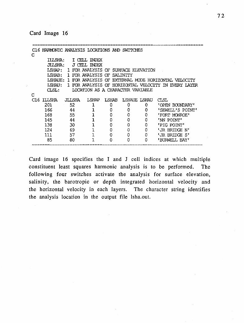
Card Image 16

Cl 6 HARMJNIC ANALYSIS IOCATIONS AND SWITOIBS C

ILLSHA: JLL.SHA: LSHAP: LSHAB:

I CELL INDEX J CELL INDEX

1 FOR ANALYSIS OF SURFACE ELEVATION 1 FOR ANALYSIS OF SALINITY

I.SHAUE: I.SHAU:

1 FOR ANALYSIS OF EXTERNAL M)DE HORIZONTAL VEUX:ITY 1 FOR ANALYSIS OF HORIZONTAL VEUX:ITY IN EVERY LAYER

CI.SL: C Cl6 ILLSHA

201 166 168 145 138 124 111

85

:U:X::ATION AS A OiARACTER VARIAB1E

JLLSHA 52 44 55 44 30 69 57 80

LSHAP 1 1 1 1 1 1 1 1

I.SHAB 0 0 0 0 0 0 0 0

LSHAUE I.SHAU 0 0 0 0 0 0 0 0 0 0 0 0 0 0 0 0

CI.SL I OPEN BOUNDARY 1

'SEWELL'S POINT' 'FORT M)NROE' 'NN POINT' 'PIG POINT' I JR BRIDGE N' 'JR BRIDGES' 'BURWELL BAY'

Card image 16 specifics the I and J cell indices at which multiple constituent least squares harmonic analysis is to be performed. The following four switches activate the analysis for surface elevation, salinity, the barotropic or depth integrated horizontal velocity and the horizontal velocity in each layers. The character string identifies the analysis location in the output file lsha.out.

72

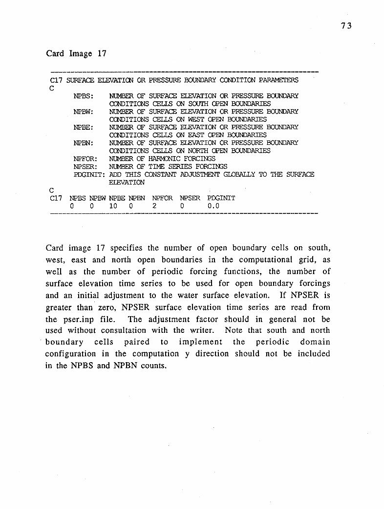
Card Image 17

Cl 7 SURFACE EIEVATICN OR PRESSURE BOUNDARY CONDITION PARAMETERS C

C

NPBS: NUMBER OF SURFACE ELEVATION OR PRESSURE BOUNDARY CONDITIONS CEU..S ON SOUI'H OPEN BOUNDARIES

NPBW: NUMBER OF SURFACE ELEVATION OR PRESSURE BOUNDARY CONDITIONS CEU..S ON WEST OPEN BOUNDARIES

NPBE: NUMBER OF SURFACE ELEVATION OR PRESSURE BOUNDARY CCNDITIONS CEU..S ON EAST OPEN BOUNDARIES

NPBN: NUMBER OF SURFACE ELEVATION OR PRESSURE BOUNDARY CONDITIONS CEU..S ON NORTH OPEN BOUNDARIES

NPFOR: NUMBER OF HARM)NIC FORCIN3S NPSER: NUMBER OF TIME SERIES FORCIN3S PDGINIT: ADD THIS CONSTANT ADJUSTMENT GLOBALLY TO THE SURFACE

EIEVATION

Cl 7 NPBS NPBW NPBE NPBN NPFOR NPSER PDGINIT 0 0 10 0 2 0 0.0

Card image 17 specifies the number of open boundary cells on south, west, east and north open boundaries in the computational grid, as well as the number of periodic forcing functions, the number of surface elevation time series to be used for open boundary forcings and an initial adjustment to the water surface elevation. If NPSER is

greater than zero, NPSER surface elevation time series are read from the pser.inp file. Th<~ adjustment factor should in general not be used without consultation with the writer. Note that south and north boundary cells paired to implement the periodic domain configuration in the computation y direction should not be included in the NPBS and NPBN counts.

73

Card Image 18

Cl8 PERIODIC FORCING SURF ELEV OR PRESSURE BOUNDARY COND. FORCINGS C

NPFOR: SYMBOL: ..AMPLITUDE:

F'ORCING NUMBER E'ORCING SYMBOL (FOR REFERENCE HERE ONLY) AMPLITUDE IN M (PRESSURE DIVIDED BY RHO*G)

PHASE: FORCING PHASE RELATIVE TO TIME ORIGIN OF TBEGIN IN SECONDS

C C18 NPFOR SYMBOL AMPLITUDE PHASE

1 'M2' 0.34200E+OO 0.10855E+05 1 'S2' 0.63000E-01 -0.13959E+05 1 'N2' 0.76000E-01 -0.11331E+05 1 'Kl' 0.44000E-01 0.21641E+05 1 'M4' 0.0 0.0 1 '01' 0.35798E-01 -0.23892E+04 1 'M6' 0.0 0.0 2 'M2' 0.0 0.0 2 'S2' 0.0 0.0 2 'N2' 0.0 0.0 2 'Kl' 0.0 0.0 2 'M4' 0.0 0.0 2 '01' 0.0 0.0 2 'M6' 0.0 0.0

Card image 18 specifies NPFOR forcing functions, each having MTIDE constituents, with the first column set to the forcing number for user reference. Constituents for each forcing should be in the order sequence defined on card image 16. The phase is specified in seconds consistent with the representation:

(4)

where , and -c are the amplitude and phase of the n constituent and ,ser is an additive time series specification of the surface elevation. The time origin for the phase should be consistent with the time origin for the simulation. For example TBEGIN on card image 8 is in Julian hours relative to midnight, January 1 of a given year. For this case, then the phase should also be relative to midnight January 1 of

74

the same year. For the analysis of field records, to accomplish this synchronization, a stand alone least square harmonic analysis program lsqhs.f is available from the writer. The null forcing function 2 might be used on an open boundary with only outgoing wave propagation, to be discussed below.

Card Image 19

Cl9 PERIODIC FORCING SURF ELEV OR PRESSURE ON SOUTH OPEN BOUNDARIES C

IPBS: JPBS: ISPBS:

NPFORS: NPSERS:

C

I CELL INDEX OF BOUNDARY CELL J CELL INDEX OF BOUNDARY CELL

1 FOR RADIATION-SEPARATION CONDITION 0 FOR EIEVATICN SPECIFIED

APPLY HARMCNIC FORCING NUMBER NPFORS APPLY TIME SERIES FORCING NUMBER NPSERS

Cl9 !PBS JPBS ISPBS NPFORS NPSERS

Card Image 20

C20 PERIODIC FORCING SURF ELEV OR PRESSURE ON WEST OPEN BOUNDARIES C

C

IPBW: SEE C'.ARD 19 JPBW: ISPBW: NPFORW: NPSERW:

C20 IPBW JPBW ISPBW NPFORW NPSERW

75

Card Image 21

C21 PERIODIC FORCING SURF ELEV OR PRESSURE ON EAST OPEN BOUNDARIES C

IPBE: SEE CARD 19 JPBE: ISPBE: NPFORE: NPSERE:

C C21 IPBE JPBE ISPBE NPFORE NPSERE

201 46 1 1 0 201 47 1 1 0 201 48 1 1 0 201 49 1 1 0 201 50 1 1 0 201 51 1 1 0 201 52 1 1 0 201 53 1 1 0 201 54 1 1 0 201 55 1 1 0

Card Image 22

C22 PERIODIC FORCING SURF ELEV OR PRESSURE ON NORTH OPEN BOUNDARIES C

C

IPBN: SEE CARD 19 JPBN: ISPBN: NPFORN: NPSERN:

C22 IPBN JPBN ISPBN NPFORN NPSERN

Card images 19 through 22 specify the open boundary conditions for the four directional faces of the horizontal computational domain. Because of the similarity of the four data sets, they will be discussed in a generic fashion. To provide back~round on the discussion of the model's operation at open boundaries, it is useful to summarize the treatment of open boundary conditions in the EFDC model. The EFDC

model provides for two types of hydrodynamic open boundary

76

conditions. The first type is the standard specification of water surface elevation using combinations of harmonic constituents and time series. The second type of open boundary conditions is referred to as a radiation-separation boundary condition in that the incoming wave at an open boundary is separated from the outgoing wave (Bennett and McIntosh, 1982). For outgoing waves the condition functions as a radiation condition with a phase speed equal to the square root of gh, where h is the mean or undisturbed depth along the open boundary. For incoming waves, 1/2 of the characteristic of the incoming wave is specified. As an example, consider an east open boundary, with the model domain to the west in the negative x

direction and the unmodeled region to the east in the positive x

direction. The incoming characteristic for the linearized onedimensional shallow water equation (Bennett, 1976), is:

,_ hu (5)

Jiii

where C is the free surface displacement, h is the water depth and u

is the x component of velocity, with the overbar denoting depth averaged or external mode velocity. For a purely progressive wave propagating in the negative x direction, incoming toward the east open boundary:

(6)

(7)

Inserting (6) and (7) into (5) gives

(7)

77

Thus 1/2 of the characteristic of the purely progressive incoming wave is the wave surface displacement.

Open boundary cells are defined by the type 5 cell type in the cell.inp file but are presumed to be external to the computation in that the continuity equation is not solved in the open boundary cell. Tangential velocities (i.e. the u or x velocity component in a south or north open boundary cell and the v or y velocity component in an east or west open boundary cell) are also not currently computed in open boundary cells. Due to the placement definition of u on west cell faces and v on south cell faces, the u is computed for east open boundary cells and v is computed for north open boundary cells. The first two parameters on each card image specify the I and J indices of the open boundary cells. The I and J indices sequence does not need to be continuous since a model domain may have multiple opening on either of the four directional face normals. The ISBPS (ISPBW,E,N) switch is set to zero for direct specification of the open boundary cell surface elevation or to 1 for the implementation of a radiationseparation boundary condition. For ISPBS set to zero, the open boundary cell water surface elevation is directly specified by the sum of the periodic forcing function (NPFORS,W,E,N) and the surface elevation time series (NPSERS,W,E,N) where NPSER_ identifies one of the NPSER surface elevation time series in the pser.inp file. The radiation-separation boundary condition specifies the linear characteristic of an assumed normal incident incoming wave as twice

the surface elevation specified by the sum of the periodic and time series forcing. By default, the outgoing characteristic is left undefined allowing waves generated interior to the model domain to pass outward across the boundary with no reflection. Since the normal incident criteria is somewhat idealized, care should be used in the use of the radiation separation boundary condition. A more sophisticated radiation-separation open boundary condition (relaxing the normal incident criteria the imposition of zero tangential velocity) is under development.

78

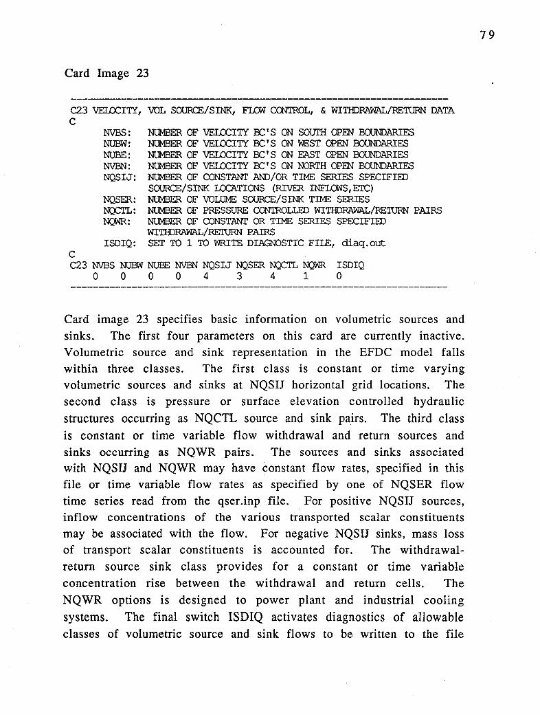
Card Image 23

C23 VELOCITY, VOL SOURCE/SINK, FLC1il CCNl'ROL, & WITHDRAWAL/RETURN DATA C

NVBS: NUBW: NUBE: NVBN: NQSIJ:

NQSER: N;X::TL: NQWR:

ISDIQ: C

NUMBER OE' VELOCITY EC' S ON SOUTH OPEN BOUNDARIES NUMBER OE' VELOCITY BC' S ON WEST OPEN BOUNDARIES NUMBER OE' VELOCITY BC' S ON EAST OPEN BOUNDARIES NUMBER OE' VELOCITY EC' S ON NORTH OPEN BOUNDARIES NUMBER OE' CONSTANT AND/OR TIME SERIES SPECIFIED SOURCE/SINK LOCATIONS (RIVER INFI.DWS,ETC) NUMBER OE' VOLUME SOURCE/SINK TIME SERIES NUMBER OE' PRESSURE CON'IROLl.ED WITHDRAWAL/RETURN PAIRS NUMBER OE' CONSTANI' OR TIME SERIES SPECIFIED WITHDRAWAL/RETURN PAIRS SET TO 1 TO WRITE DIAGNOSTIC FILE, d.iaq.out

C23 NVBS NUBW NUBE NVBN NQSIJ NQSER NQCTL NQWR ISDIQ 0 0 0 0 4 3 4 1 0

Card image 23 specifies basic information on volumetric sources and sinks. The first four parameters on this card are currently inactive. Volumetric source and sink representation in the EFDC model falls within three classes. The first class is constant or time varying volumetric sources and sinks at NQSIJ horizontal grid locations. The second class is pressure or surface elevation controlled hydraulic structures occurring as NQCTL source and sink pa_irs. The third class is constant or time variable flow withdrawal and return sources and sinks occurring as NQWR pairs. The sources and sinks associated with NQSIJ and NQWR may have constant flow rates, specified in this file or time variable flow rates as specified by one of NQSER flow time series read from the qser.inp file. For positive NQSIJ sources, inflow concentrations of the various transported scalar constituents may be associated with the flow. For negative NQSIJ sinks, mass loss of transport scalar constituents is accounted for. The withdrawalreturn source sink class provides for a constant or time variable concentration rise between the withdrawal and return cells. The NQWR options is designed to power plant and industrial cooling systems. The final switch ISDIQ activates diagnostics of allowable classes of volumetric source and sink flows to be written to the file

79

diaq.out. Since this file can become quite large, this option is recommended to be used only for debugging. Generally when activated, the model should be allowed to run only a few timesteps and then killed.

Card Image 24

C24 VOLUME SOURCE/SINK LOCATIONS, MAGNITUDES, AND CONCENTRATION SERIES C

IQS: JQS: QSSE: N(1,1UL:

N<.J,1F:

NQSERQ: NSSERQ: NTSERQ: NDSERQ: NSDSERQ: NSWSERQ:

C

I CELL INDEX OF VOLUME SOURCE/SINK J Cifil. INDEX OF VOLUME SOURCE/SINK CONSTAN'I' INFI.DW/OUTFLOW RATE IN M*M*M/S or M*M/S MUL'fIPLIER SWITCH FOR CONSTANT AND TIME SERIES VOL S/S = 0 MULT BY 1. FOR NOFMAL IN/OUTFLOW (L*L*L/T) = 1 MJLT BY DY FOR IATERAL IN/OUTFLOW (L*L/T) CN

U F'.ACE = 2 MULT BY DX FOR IATERAL IN/OUTFLOW (L*L/T) CN

V F'.ACE = 3 MULT BY DX+DY FOR IATERAL IN/OUTFLOW (L*L/T)

ON U&V FACES IF N:)N ZERO ACCOUNT FOR VOL S/S MOMENTUM FLUX = 1 M)MENT(JM FLUX CN NEG U FACE = 2 MCMENTCJM FLUX CN NEG V FACE = 3 M)MENT(JM FLUX CN POS U FACE = 4 M)MENT(JM FLUX CN POS V FACE

ID NUMBER OF ASSOCIATED VOLUMN FLOW TIME SERIES ID NUMBER OF ASSOCIATED SALINITY TIME SERIES ID NUMBER OF ASSOCIATED TEMPERATURE TIME SERIES ID NUMBER OF ASSOCIATED DYE CCNC TIME SERIES ID NUMBER OF ASSOCIATED SEDIMENT CONC TIME SERIES ID NUMBER OF ASSOCIATED SAL WATER QUALITY TIME SERIES

C24 IQS JQS QSSE NGMUL NCMF NQSERQ NSSERQ NTSERQ NDSERQ NSDSERQ NSWSERQ 191144 0.0 0 0 1 0 1 0 0 0 112 6 0.0 0 0 2 0 1 0 0 0 112 7 0.0 0 0 3 0 1 0 0 0 100 100 1.0 0 0 0 0 0 0 0 0

Card image 24 provides information for the NQSIJ class of volumetric source sink flows, with the first two parameters specifying the location by I and J indices. The third parameter, QSSE is used to specify a time invariant inflow rate ( outflows or sinks simply have negative signs) in either cubic meters per second or cubic meters per second per meter. The adjustment factor NQMUL specifies how

80

volumetric flows per unit length are converted to true volumetric flows. The control ]Parameter NQMF indicates if the volumetric source or sink is to have an associated momentum flux ·and which face of the source cell the momentum flux is assigned. Time variable flows are defined by entering a flow time series identifier number (less than or equal to NQSER) under NQSERQ. The remaining five columns allow the specification of a scalar constituent concentration time series associated with the flow time series only. Constant concentrations associated with the constant QSEE flows are defined on card image 25, below. The constant flowrate source and sinks are distributed uniformly over the vertical layers, while the time series specification of source and sink flows allows arbitrary distribution over the vertical layers.

Card Image 25

C25 TIME CONSTANT INFLOW CONC FOR TIME CONSTANT VOLUMETRIC SOURCES C

C

SALT: SALT CCNCENTRATION CXlRRESPONDING 'ID INFLOW ABOVE TEMP: TEMPERATURE CORRESPONDING TO INFLOW ABOVE DYEC: DYE CCNCENTRATION CORRESPONDING 'ID INFLOW ABOVE SEDC: SEDIMENT CONCENTRATION CORRESPONDING TO INFLOW ABOVE SFL SFL CCNCENTRATION CORRESPONDING 'ID INFLOW ABOVE

C25 SALT TEMP DYEC SEDC SFL 0. 0. 0. 0. 0. 0. 0. 0. 0. 0. 0. 0. 0. 0. 0. 0. 20. 0. 0. 0.

8 1

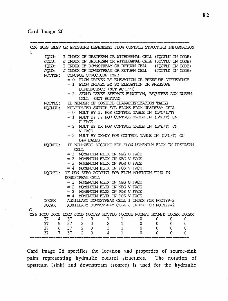
Card Image 26

C26 SURF ELEV OR PRESSURE DEPENDENT FLa'l CONTROL STRUCTURE INFORMATION C

C

IQLU: JQLU: IQI.D: JQI.D: N(CTYP:

NQCTLQ: NC(MUL:

NC(ME'U:

NC(MFD:

IQCAX JQCAX

I INDEX OF UPSTREAM OR WITHDRAWAL CELL J INDEX OF UPSTREAM OR WITHDRAWAL CELL I INDEX OF DOWNSTREAM OR RETURN CELL J INDEX OF DOWNSTREAM OR RETURN CELL

CONTROL STRtx::TURE TYPE

(I<;X:TLU IN CODE) (JCCTLU IN CODE) (ICCTI.D IN CODE) (JCCTI.D IN CODE)

= 0 El..OW DRIVEN BY EI.EVATION OR PRESSURE DIFFERENCE = l El..OW DRIVEN BY SQ ELEVATION OR PRESSURE

DIFFERCENCE (NOT ACTIVE) = 2 SEWMD LEVEE SEEPAGE FUNCTION, REQUIRES AUX DNSRM

CELL (IDT ACTIVE) ID NUMBER OF CONI'ROL OIARACTERIZATION TABLE MULTIPLIER SWITOI FOR FLOWS FRCM UPSTREAM CELL = 0 MlJLT BY 1. FOR CONTROL TABLE IN (L*L*L/T) = l MlJLT BY DY FOR CONTROL TABLE IN (L*L/T) CN

U FACE = 2 MlJLT BY DX FOR CONTROL TABLE IN (L*L/T) CN

V FACE = 3 MlJLT BY DX+DY FOR CONTROL TABLE IN (L*L/T) CN

U&V FACES IF NON--ZERO ACCOUNT FOR FLOW MCMENTUM FLUX IN UPSTREAM

CEI.J. = l M::MENTUM FLUX CN NEG U FACE = 2 M::MENTUM FLUX CN NEG V FACE = 3 MCMENTUM FLUX CN POS U FACE = 4 M::MENTUM FLUX CN POS V FACE

IF IDN ZERO ACCOUNT FOR FLOW M:MEN'TIJM FLUX IN DOWNSTREAM CELL = 1 M::MENTUM FLUX CN NEG U FACE = 2 M::MENTUM FLUX CN NEG V FACE = 3 M::MENTIJM FLUX ON POS U FACE = 4 MCMENTUM FLUX CN POS V FACE AUXILIARY DOWNSTREAM CELL I INDEX FOR NOCTYP=2 AUXILIARY DOWNSTREAM CELL J INDEX FOR NOCTYP=2

C26 ICPJ JCPJ ICQ) JCQ) NCCTYP NOCTLQ N<XMUL NC(MFU NQ:MFD IQCAX JQCAX 37 4 37 2 0 1 1 0 0 0 0 37 5 37 2 0 2 1 0 0 0 0 37 6 37 2 0 3 1 0 0 0 0 37 7 37 2 0 4 1 0 0 0 0

Card image 26 specifies the location and properties of source-sink pairs representing hydraulic control structures. The notation of upstream (sink) and downstream (source) is used for the hydraulic

82

control structure pairs, which allow flow in only one direction. For structures such as culverts, which allow bi-directional flow, two control structure pairs are necessary to account for both flow directions. The first four parameters on this card image define the horizontal locations by the I and J indices of the upstream and downstream cells. Structures whose flowrates depend only on the surface elevation in the upstream cell (i.e., spillways and weirs) can discharge out of the computational domain by specifying the null indices 0,0 for the downstream cell. The parameter NQCTYP specifies the form of the flow dependence on the surface elevation difference between the upstream and downstream cell, (with only the O option currently active). The parameter NQCTLQ identifies control table number characterizing the structure. The control tables are input in the file qctl.inp. The options identifies NQCMUL and NQCMFU are similar to those discussed for the NQSIJ class sources and sinks. The remaining two indices, IQCAX and JQCAX are currently not used.

Card Image 27

C27 FLOW WITHDRAWAL, HEAT OR MATERIAL ADDITION, AND RETURN DATA. C

IWU: JWU: IWRD: JWRD: CWRE: NQSERW: NSSERW: NTSERW: NDSERW: NSDSERW: NSFSERW:

C

I INDEX OF UPSTREAM OR WITHDRAWAL CELL (IWRU IN CODE) J INDEX OF UPSTREAM OR WITHDRAWAL CELL (IWRU IN CODE) I INDEX OF DOWNSTREAM OR RETURN CELL (IWRD IN CODE) J INDEX OF DOWNSTREAM OR RETURN CELL (IWRD IN CODE) CONSTANT VOLUMN FLOW RATE FRCM WITHDRAWAL TO RETURN ID NUMBER OF ASSOCIATED VOLUMN FLOW TIME SERIES ID NUMBER OF ASSOCIATED SALINITY INCREASE TIME SERIES ID NUMBER OF ASSOCIATED TEMP INCREASE TIME SERIES ID NUMBER OF ASSOCIATED DYE CONC INCREASE TIME SERIES ID NUMBER OF ASSOCIATED SED CONC INCREASE TIME SERIES ID NUMBER OF ASSOCIATED SFL CONC INCREASE TIME SERIES

C27 IWU JWU IWD JCWD QWRE NQSERW NSSERW NTSERW NDSERW NSDSERW NSFSERW 84 102 75 107 88.3 0 0 0 0 0 0

Card image 27 provides information for the NQWR volumetric source-sink class with the location of the upstream (withdrawal) and downstream (return) flow cell pairs specified by their I and J indices. The remaining parameters specify a constant flow rate and time

83

series identified for variable flow rates and concentration rises. Time constant concentration rises associated with the constant flow rate are specified as shown below on card image 28.

Card Image 28

C28 TIME CONSTANT WITHDRAWAL AND RETURN CONCENTRATION RISES C

SALT: SALINITY RISE TEMP: TEMl?ERA'l'URE RISE DYE: DYE CONCENTRATION RISE SEDC: SEDIMENT CONCENTRATION RISE SFL: SFL RISE

C C28 SALT TEMP DYEC SEDC SFL

0. 8. 0. 0. 0.

84

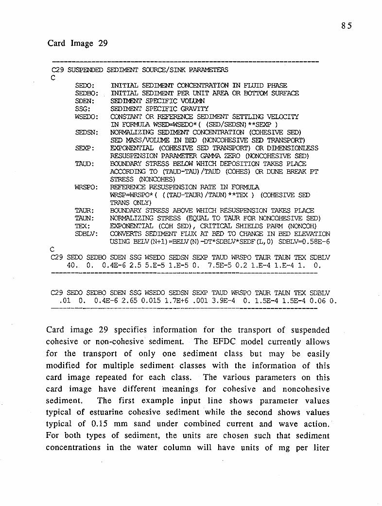
Card Image 29

C29 SUSPENDED SEDIMENT SOURCE/SINK PARAMETERS C

C

SEDO: SEDBO: SDEN: SSG: WSEDO:

SEDSN:

SEXP:

TAUD:

WRSPO:

TAUR: TAUN: 'IEX: SDBLV:

INITIAL SEDIMENT CONCENTRATION IN FllJID PHASE INITIAL SEDIMENT PER UNIT AREA OR BOTTCM SURFACE SEDil-E'IT SPECIFIC VOUMl SEDIMEN'I' SPECIFIC GRAVITY CONSTANT OR REFEREOCE SEDIMENT SETTLING VELOCITY IN FORMCn.A WSED=WSEDO* ( (SED/SEDSN) **SEXP ) NORMALIZING SEDIMENT CONCENTRATION (COHESIVE SEO) SEO MASSNOUJME IN BED (NONCOHESIVE SEO TRANSPORT) EXPONENTIAL (COHESIVE SEO TRANSPORT) OR DIMENSIONIESS RESUSPENSION PARAMETER GAMMA ZERO (IDNCOHESIVE SEO) BOUNDARY STRESS BELOW WHICH DEPOSITION TAKES PLACE ACCORDING TO (TAUD-TAU) /TAUD (COHES) OR DUNE BREAK PT STRESS (NONCOHES) REFERENCE RESUSPENSION RATE IN FORMCn.A WRSP=WRSPO* ( ( (TAU-TAUR) /TAUN) **'IEX ) (COHESIVE SEO TRANS ONLY) BOUNDARY STRESS ABOVE WHICH RESUSPENSION TAKES PLACE NORMALIZING STRESS (EQUAL TO TAUR FOR NONCOHESIVE SEO) EXPONENTIAL (COH SEO), CRITICAL SHIEIDS PARM (NONCOH) CONVERTS SEDIMENT FLUX AT BED TO CHANGE IN BED ElEVATION USING BEIN (N+ 1) =BELV (N) -DT*SDBLV*SEDF (L, 0) SDBLV=O. 58E-6

C29 SEDO SEDBO SDEN SSG WSEDO SEDSN SEXP TAUD WRSPO TAUR TAUN 'IEX SDBLV 40. 0. 0.4E-6 2.5 5.E-5 1.E-5 0. 7 .5E-5 0.2 1.E-4 1.E-4 1. 0.

C29 SEDO SEDBO SDEN SSG WSEDO SEDSN SEXP TAUD WRSPO TAUR TAUN 'IEX SDBLV .01 0. 0.4E-6 2.65 0.015 1.7E+6 .001 3.9E-4 0. 1.5E-4 1.5E-4 0.06 0.

Card image 29 specifies information for the transport of suspended cohesive or non-cohesive sediment. The EFDC model currently allows for the transport of only one sediment class but may be easily modified for multiple sediment classes with the information of this card image repeated for each class. The various parameters on this card image have different meanings for cohesive and noncohesive sediment. The first example input line shows parameter values typical of estuarine cohesive sediment while the second shows values typical of 0.15 mm sand under combined current and wave action. For both types of sediment, the units are chosen such that sediment concentrations in the water column will have units of mg per liter

85

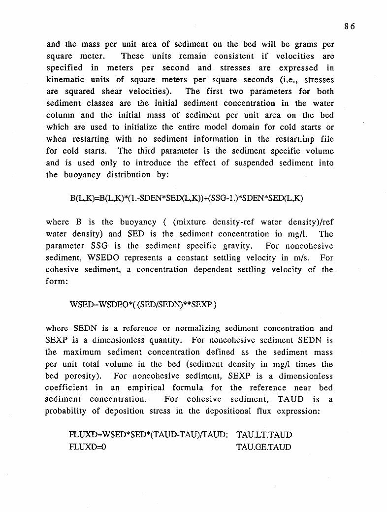
and the mass per unit area of sediment on the bed will be grams per square meter. These units remain consistent if velocities are specified in met,~rs per second and stresses are expressed in kinematic units of square meters per square seconds (i.e., stresses are squared shear velocities). The first two parameters for both sediment classes are the initial sediment concentration in the water column and the initial mass of sediment per unit area on the bed which are used to initialize the entire model domain for cold starts or when restarting with no sediment information in the restart.inp file for cold starts. The third parameter is the sediment specific volume and is used only to introduce the effect of suspended sediment into the buoyancy distribution by:

B(L,K)=B(L,K)*(l .-SDEN*SED(L,K))+(SSG-1.)*SDEN*SED(L,K)

where B is the buoyancy ( (mixture density-ref water density)/ref water density) and SED is the sediment concentration in mg/1. The parameter SSG is the sediment specific gravity. For noncohesive sediment, WSEDO represents a constant settling velocity in m/s. For cohesive sediment, a concentration dependent settling velocity of the form:

WSED=WSDEO*( (SED/SEDN)**SEXP)

where SEDN is a reference or normalizing sediment concentration and SEXP is a dimensionless quantity. For noncohesive sediment SEDN is the maximum sediment concentration defined as the sediment mass per unit total volume in the bed (sediment density in mg/1 times the bed porosity). For noncohesive sediment, SEXP is a dimensionless coefficient in an empirical formula for the reference near bed sediment concentration. For cohesive sediment, TAUD is a probability of deposition stress in the depositional flux expression:

FLUXD=WSED*SED*(TAUD-TAU)/fAUD: TAU.LT.TADD FLUXD=O TAU.GE.TADD

86

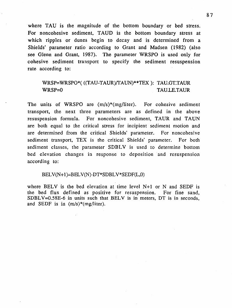
where TAU is the magnitude of the bottom boundary or bed stress. For noncohesive sediment, TAUD is the bottom boundary stress at which ripples or dunes begin to decay and is determined from a Shields' parameter ratio according to Grant and Madsen (1982) (also see Glenn and Grant, 1987). The parameter WRSPO is used only for cohesive sediment transport to specify the sediment resuspension rate according to:

WRSP=WRSPO*( ((TAU-TAUR)/I'AUN)**TEX ): TAU.GT.TAUR WRSP=O TAU.LE.TAUR

The units of WRSPO are (m/s)*(mg/liter). For cohesive sediment transport, the next three parameters are as defined in the above resuspension formula. For noncohesive sediment, TAUR and TAUN are both equal to the critical stress for incipient sediment motion and are determined from the critical Shields' parameter. For noncohesive sediment transport, TEX is the critical Shields' parameter. For both sediment classes, the parameter SDBLV is used to determine bottom bed elevation changes in response to deposition and resuspension according to:

BELV(N+ l)=BEL V(N)-DT*SDBLV*SEDF(L,0)

where BELV is the bed elevation at time level N+l or N and SEDF is the bed flux defined as positive for resuspension. For fine sand, SDBLV=0.58E-6 in units such that BELY is in meters, DT is in seconds, and SEDF is in (m/s)*(mg/liter).

87

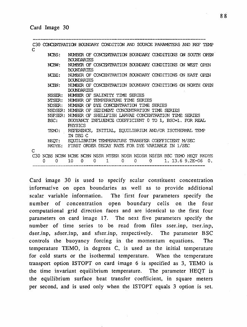
Card Image 30

C30 CON:ENI'RATION BOUNDARY CONDITION AND SOURCE PARAMETERS AND REF TEMP C

N:BS:

N::BW:

N::BE:

N:BN:

NSSER: NTSER: NOSER: NSDSER: NSFSER: B.SC:

TEMJ:

HEQT: RKDYE:

C

NUMBER OF CONCENTRA'.rION OOUNDARY CONDITICNS ON SOOTH OPEN BOUNDARIES NUMBER OF CONCENTRATION OOUNDARY CONDITIONS ON WEST OPEN BOUNDARIES NUMBER OF' CONCEN'I'RN.rION OOUNDARY CONDITIONS ON EAST OPEN BOUNDARIES NUMBER OF' CONCENTRA'.rION OOUNDARY CONDITICNS ON NORTH OPEN BOUNDARIES NUMBER OF SALINITY TIME: SERIES NUMBER OF TEMPERATURE TIME: SERIES NUMBER OF DYE CONCENTRATICN TIME: SERIES NUMBER OF SEDIMENT CONCENTRATION TIME: SERIES NUMBER OF SHELlF.ISH LARVAE CONCENTRATION TIME: SERIES BUOYANCY INFLUENCE COEFFICIENT O TO 1, BSC=l. FOR REAL PHYSICS REFERENO~, INITIAL, EQUILIBRIUM AND/OR ISOTHERMAL TEMP IN DEG C EQUILIBRIUM TEMPERATURE TRANSFER COEFFICIENT M/SF.C FIRS'r ORDER DECAY RA.TE FOR DYE VARIABLE IN 1/SEC

C30 NCB.5 NCBW NCBE NCBN NSSR NTSEI~ NDSR NSDSR NSfSR BSC TEMJ HEQT RKDYE 0 0 10 0 0 1 0 0 0 1. 13.6 9.2E-06 0.

Card image 30 is used to specify scalar constituent concentration informative on open boundaries as well as to provide additional scalar variable information. The · first four parameters specify the

number of concentration open boundary cells on the four computational grid direction faces and are identical to the first four parameters on card image 17. The next five parameters specify the number of time series to be read from files sser.inp, tser.inp, dser.inp, sdser.inp, and sfser.inp, respectively. The parameter BSC controls the buoyancy forcing in the momentum equations. The temperature TEMO, in degrees C, is used as the initial temperature for cold starts or the isothermal temperature. When the temperature transport option ISTOPT on card image 6 is specified as 3, TEMO is the time invariant equilibrium temperature. The parameter HEQT is the equilibrium surface heat transfer coefficient, in square meters

per second, and is used only when the ISTOPT equals 3 option is set.

88

The remaining parameter RKDYE is a first order decay rate of the dye tracer variable and must have units of I/seconds.

Card Image 31

C31 LOCATION OF CONC BC' S ON SOU'I'H BOUNDARIES C

C

ICBS: I CELL INDEX JCBS: J CELL INDEX NI'SCRS: NUMBER OF TIME STEPS 'ID RECOVER SPECIFIED VALUES ON

OIANGE 'I'O ~ FRa.1 OU'I'FlDW NSSERS: SOUTH BOUNDARY CEIJ, SALINITY TIME SERIES ID NUMBER NI'SERS: SOUTH BOUNDARY CEIJ, TEMPERATURE TIME SERIES ID NUMBER NDSERS: SOUTH BOUNDARY CEIJ, DYE CONC TIME SERIES ID NUMBER NSDSERS: SOUTH BOUNDARY CEIJ, SED CONC TIME SERIES ID NUMBER NSWSERS: SOUTH BOUNDARY CEIJ, SE'L CONC TIME SERIES ID NUMBER

C31 IBBS JBBS NTSCRS NSSERS NTSERS NDSERS NSDSERS NSWSERS

Card Image 32

C32 TIME CONSTANT BOTTa.1 CONC ON SOUTH CCNC BOUNDARIES C

C

SALT: ULTIMATE INFLOWING BOTTa.1 1AYER SALINITY TEMP: ULTIMATE INFI.DWIN; BOTTa.1 LAYER TEMPERATURE DYEC: ULTIMATE INFLOWING BCYI'TCM LAYER DYE CONCENTRATICN SEDC: UL'l'IMATE INFI.DWING BC>TTa.1 LAYER SEDIMENT CONCENTRATION SFL: ULTIMATE INFLOWING BCYI'TCM LAYER SFL CONCENTRATICN

C32 SALT TEMP DYF..C SEDC SFL

89

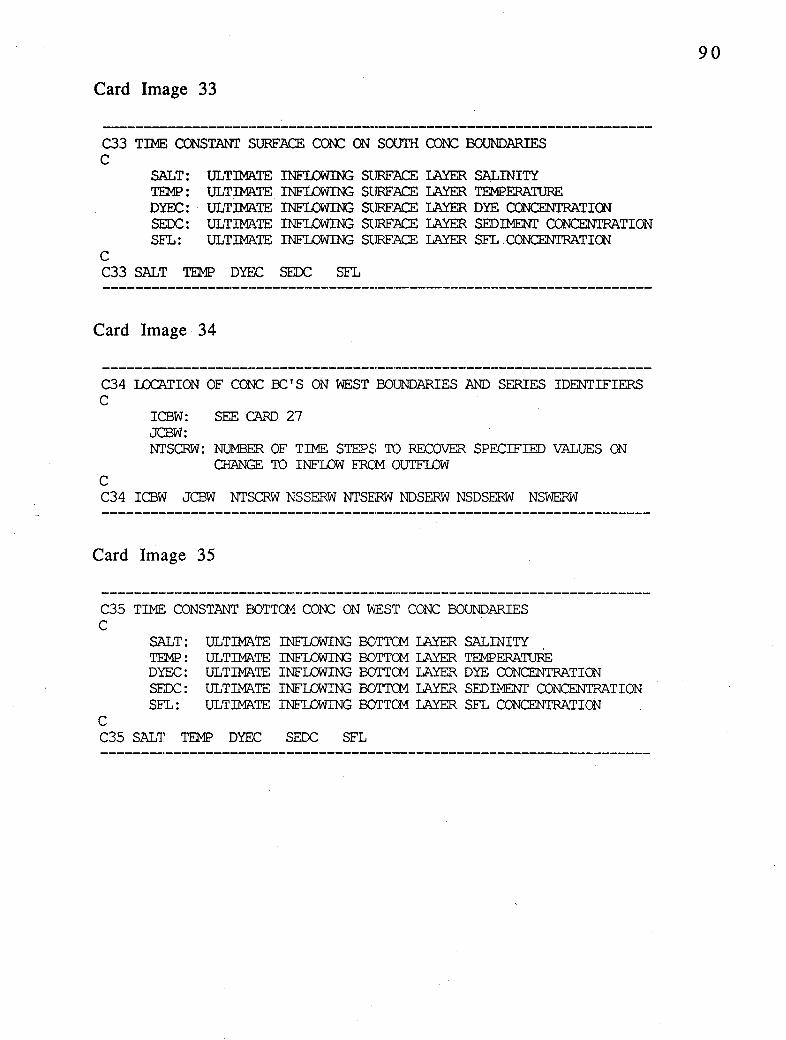
Card Image 33

C33 TIME CONSTANT SURFACE cm: ON SOOI'H CONC BOUNDARIES C

C

SALT: ULTIMATE INFLOWING SURFACE LAYER SALINITY TEMP: ULTIMATE INFLOWING SURFACE LAYER TEMPERATURE DYEC: ULTIMA.TE INFLOWING SURFACE LAYER DYE CONCENTRATICN SECC: ULTIMATE INFLOWING SURFACE LAYER SEDIMENT CONCENTRATION SFL: ULTIMATE INFLOWING SURFACE LAYER SFL . CONCENTRATICN

C33 SALT TEMP DYEC SEDC SFL

Card Image 34

C34 L<X:ATION OF CONC :oc:' S ON WEST BOUNDARIES AND SERIES IDENTIFIERS C

C

ICBW: SEE CARD 27 JCBW: NTSCRW: NUMBER OF' TIME STEPS TO RECOVER SPECIFIED VALUES ON

OlANGE TO INFLOW FRCM OUTFI.DW

C34 ICBW JCBW NTSffiW NSSERW NTSERW NDSERW NSDSERW NSWERW

Card Image 35

C35 TIME CONSTANT BOTTCM CON: ON WEST CONC BOUNDARIES C

C

SALT: ULTIMA'IE INFLOWING BOTTCM LAYER SALINITY TEMP: ULTIMATE INFI..OWIN:; BOTTCM LAYER TEMPERATURE DYEC: ULTIMATE INFLOWING BOTTCM LAYER DYE CONCENTRATION SEDC: ULTIMA'IE INFLOWING BOTTCM LAYER SEDIMENT CONCENTRATION SFL: ULTIMATE INFLOWING BOTTCM LAYER SFL CONCENTRATION

C35 SAL1' TEMP DYEC SECC SFL

90

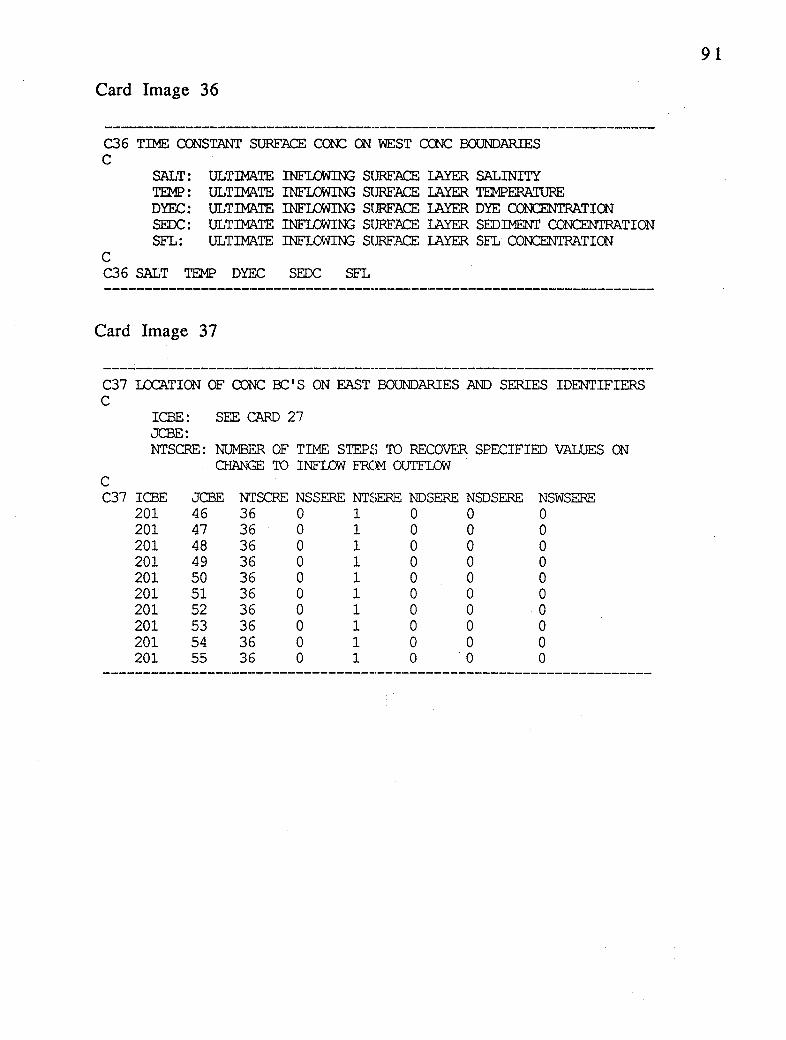
Card Image 36

C36 TIME CONSTANT SURFl~ COOC ON WEST CCNC BOUNDARIES C

SALT: ULTIMA.TE INFLOWING SURFACE 1AYER SALINITY TEMP: ULTIMA.TE INFLOWING SURFACE LAYER TEMPERATURE DYEC: ULTIMA.TE INFLOWING SURFACE LAYER DYE CONCENTRATICN SEDC: ULTIMA.TE INFLOWING SURFACE IAYER SEDIMENT CONCENTRATION SFL: ULTIMA.'IE INFLOWING SURFACE LAYER SFL CONCENTRATICN


Card Image 37

C37 LCCATION OF CONC BC' S ON EAST BOUNDARIES AND SERIES IDENTIFIERS C

ICBE: SEE ('.ARD 27 JCBE: NTSCRE: NUMBER OF TIME STEPS 'ID RECOVER SPECIFIED VALUES ON

CHANGE TO INFLOW FRC:M OUTFIOW C C37 ICBE

201 201 201 201 201 201 201 201 201 201

JCBE 46 47 48 49 50 51 52 53 54 55

NTSCRE NSSERE NTSERE NDSERE NSDSERE 36 0 1 0 0 36 0 1 0 0 36 0 1 0 0 36 0 1 0 0 36 0 1 0 0 36 0 1 0 0 36 0 1 0 0 36 0 1 0 0 36 0 1 0 0 36 0 1 0 0

NSWSERE 0 0 0 0 0 0

.Q

0 0 0

91

Card Image 38

C38 TIME COOSTANT BOTTCM CON: ON l~T CCNC BOUNDARIES C

C

SALT: ULTIW\'IE INFI.OWING BOTTCM IAYER SALINITY TEMP: ULTIW\'IE INF1DWIN3 BOTTCM I.AYER TEMPERATURE DYEC: ULTIW\'IE INFI.OWING BOTTCM I.AYER DYE CONCENTRATICN SEDC: ULTIW\'IE INFI.DWING BOTTCM I.AYER SEDIMENT CONCENTRATION SFL: ULTIW\'IE INFI.OWING BOTTCM I.AYER SFL CONCENTRATICN

C38 SALT TEMP DYr::X: SEDC SFL 30. 25.6 0. 0. 30. 30. 25.6 0. 0. 30. 30. 25.6 o. 0. 30. 30. 25.6 o. 0. 30. 30. 25.6 0. 0. 30. 30. 25.6 0. 0. 30. 30. 25.6 o. 0. 30. 30. 25.6 o. 0. 30. 30. 25.6 0. 0. 30. 30. 25.6 0. 0. 30.

Card Image 3 9

C39 TIME CONSTANT SURFACE CON: ON EAST CCNC BOUNDARIES C

C

SALT: ULTIMA.'IE INFLOWING SORFACE IAYER SALINITY TEMP: ULTIMA.'IE INFLOWING SURF.ACE I.AYER TEMPERATURE DYEC: ULTIMA.'IE INFLOWING SORFACE I.AYER DYE CONCENTRATICN SEDC: ULTIMZ\.'IE INFLOWING SURFACE IAYER SEDIMENT CONCENTRATION SFL: ULTIMA.'IE INFLOWING SURFACE I.AYER SFL CONCENTRATICN

C39 SALT TEMP DYEC SEDC SFL 30. 25.6 0. 0. 30. 30. 25.6 0. 0. 30. 30. 25.6 0. 0. 30. 30. 25.6 0. o. 30. 30. 25.6 0. 0. 30. 30. 25.6 0. 0. 30. 30. 25.6 0. 0. 30. 30. 25.6 0. 0. 30. 30. 25.6 0. 0. 30. 30. 25.6 0. 0. 30.

92

Card Image 40

C40 LCCATION OF CONC B'.::' S ON NORTH BaJNDARIES AND SERIES IDENTIFIERS C

C

ICBN: SEE CARD 27 JCBN: NTSCRN: NUMBER OF TIME STEPS TO RECOVER SPECIFIED VALUES CN ~ TO INFLOW FRCM OUTFLOW

C40 ICBN JCBN NTSCRN NSSERN NTSERN NDSERN NSDSERN NSWERN

Card Image 41

C41 TIME CONSTANT BOTTCM CONC ON NORTH CCNC BOUNDARIES C

SALT: ULTIMATE INFLOWING BOTTCM IAYER SALINITY TEMP: ULTIMATE INFLOWIN:; BOTTCM IAYER TEMPERATURE DYEC: ULTIMA'IE INFLOWING BOTTCM IAYER DYE CONCENTRATICN SEDC: ULTIMA'IE INFLOWING BOTT<l1 LAYER SEDIMENT CONCENTRATION SFL: ULTIMA'IE INFLOWING BOTTCM LAYER SFL CONCENTRATICN

C41 SALT TEMP DYEC SEDC SFL

Card Image 42

C42 TIME CONSTANT SURFACE CON:: ON NORTH CONC BOUNDARIES C

SALT: ULTIMATE INFLOWING SURFACE IAYER SALINITY TEMP: ULTIMATE INFLOWING SlJRFACE LAYER TEMPERATURE DYEC: ULTIMA'IE INFLOWING SORFACE IAYER DYE CONCENTRATICN SEDC: ULTIMA'IE INFLOWING SURFACE LAYER SEDIMENT CONCENTRATION SFL: ULTIMA'IE INFLOWING SURFACE LAYER SFL CONCENTRATICN


93

Card images 31 through 42 specify scalar inflowing concentrations on open boundaries. The open boundary condition for salinity, temperature and other transported constituents is based on the specification of inflowing values. The inflowing values may be specified as depth dependent and either time constant or time variable, if concentration time series are available at open boundaries. Outflowing values are calculated using upwinded values immediately inside the open boundary. When the flow at the open boundary changes from outflow to inflow, the model provides for a linear interpolation of inflowing concentration, over a user specified

. number of timesteps, (NTSCR_ on card images 31, 34, 37, and 40) between the last outflowing value and the of concentration, which allows for a concentration values at the open boundary.

ultimate inflowing value smooth transition of The ultimate inflowing

concentration is the sum of a time constant value and a time series specified inflowing concentration value (either of which may be zero). Card images 31, 34, 37, and 40 define the location of open boundary cells by the indices ICB_ and JCB_. The next parameter on these four card images, NTSCR_, defines the number of time steps to recover the specified boundary concentration value after the change from outflow to inflow. For tidal flows, NTSCR_ might typically be the number of time steps corresponding to one hour. Alternately NTSCR_ can be adjusted during model calibration. The remaining five parameters on these four cards specify scalar concentration time series identifier numbers if the inflow concentrations are to be specified by time series. The time series specification of inflowing concentrations allows a unique concentration in each layer of the boundary cell. When the open boundary inflow concentrations are specified by constant values, bottom layer values on the four computational domain face directions are specified on card images 32, 35, 38, and 41, while surface layer values are specified on card images 33, 36, 39, and 42. If the number of layers exceeds two, values for the interior layers are linearly interpolated between the bottom and surface layer values.

94

Card Image 43

C43 DRIFTER DATA (1ST 4 DATA FOR SUB DRIFTER, 2ND 6 FOR SUB I.AGRES) C

C

ISPD:

NPD: NPDRT: NWPD:

ISLRD: 1

ILRDl ILRD2 JLRDl JLRD2 MLRDRT IPLRD

1 TO ACTIVATE SIMULTANEOUS RELEASE AND LAGRANGIAN TRANSPORT OF NEUTRALLY BUOYANT PARTICLE DRIFTERS AT I.OCATIONS INPUT ON C44 NUMBER OF PARTICLE DRIFTERS TIME: STEP AT WHIOI PARTICLES ARE RELEASED NUMBER OF TIME STEPS BETWEEN WRITING TO TRACKING FIIE drifter.out TO ACTIVATE CAI.CUIATION OF LAGRANGIAN MEAN VELOCITY OVER TIME INI'ERVAL TREF AND SPATIAL INI'ERVAL ILRPD1<I<ILRPD2, JLRD1<J<JLRD2, l<K<KC, WITH MIBPDRT RELEASES. AN AVERAGE OVER ALL RELEASE TIMES IS ALSO CALCUIATED

2 SAME: AS 1 BUT USES HIGHER ORDER TRAJECTORY INTEGRATION 3 SAME: AS 1 BUT AVERAGE OF RELEASES IS RELCX:ATED TO

TRAJECTORY BARYCEN'IER 4 SAME AS 3 BUT USES A HIGHER ORDER TRAJECTORY INTEGRATION

WEST BOUNDARY OF REGION EAS'l' BOUNDARY OF REGION NORTH BOUNDARY OF REGION SOUTH BOUNDARY OF REGION NUMBER OF RELEASE TIMES 1,2,3 WRITE FILES TO PLOT ALL, EVEN, OR

ODD HORIZONTAL CELL LAG VEL VECTORS

C43 ISPD NPD NPDRT NWPD ISLRD ILRDl ILRD2 JLRDl JLRR2 MLRPDRT IPLRD 1 4 1260 12 3 80 170 20 100 12 1

Card image 43 activates and controls two types of Lagrangian

particle trajectory calculations, which may be simultaneously activated. The first Lagrangian trajectory calculation, activated by ISPD=l, releases NPD particles at time step NPDRT. The released particles are then tracked for the remainder of the model simulation, with the nearest cell center positions (l,J,K) written to the file drifter.out every NWPD time steps. The initial position of the NPD particles is specified on card image 44, shown below. The second Lagrangian trajectory calculation, activated by ISLRD greater than zero, releases particles at active water cell centers for all vertical

layers, in the region of the computational grid bound in the x or I direction by (ILRD1.LE.I.LE.ILRD2), and in the y or J direction by

95

(JLRD1.LE.J.LE.JLRD2). MLRPDRT releases, evenly spaced in the reference time period, card 8, occur during the next to last reference time period of the model simulation (i.e., NTC.GE.2). Each group of particles is tracked for one reference time period and their net vector displacements from their release positions are determined. The net vector displacements are then divided by the reference time period to give Lagrangian mean velocity vectors (Hamrick, 1994a), which are written to the file lmvvech.out. The average Lagrangian mean of the MLRPDRT release times is also calculated and written to the file almvvech.out. For ISLRD equal to 1 or 2, the Lagrangian mean velocity vectors are associated with their release positions for plotting. For ISLRD equal to 3 or 4, the Lagrangian mean velocity vectors are associated with the mean position of the corresponding particle during its trajectory. To assure a uniform distribution of vectors for plotting, the trajectory centroid located vectors are interpolated back to the cell centers and the results written to the file lmvech.out for the MLRPDRT releases with the average of the releases written to the file almvech.out. Values of 1 or 3 for ISLRD implement first order explicit forward Euler integrator for the trajectory calculation, while values of 2 and 4 implement a second order implicit trapezoidal integrator (Bennett and Clites, 1987) incurring increased computational time. If the trajectory calculation is executed over the entire grid for 10 to 12 release times, the computational effort for the last two time cycles is increased by approximately 20 to 40 percent.

96

Card Image 44

C44 INITIAL DRIFTER POSITIONS (FOR USE WITH SUB DRIFTER) C

C

RI: I CELL INDEX IN WHICH PARTICLE IS RELEASED IN RJ: J CELL INDEX IN WHICH PARTICLE IS RELEASED IN RK: K CELL INDEX IN WHICH PARTICLE IS RELEASED IN

C44 RI RJ RK

44 6 45 6

146 147

Card Image 45

C45 CONSTANTS FOR CARTESIAN GRID CELL CENTER LONGITUDE AND LATITUDE C

Q)LONl: Q)LON2: Q)LON3: Q)lATl: CD1AT2: CD1AT3:

C

6 CONSTANTS TO GIVE CELL CENTER lAT AND LON OR OTHER COORDINATES FOR CARTESIAN GRIDS USING THE FORMULAE DLON(L)=O)LON1+(CDLON2*FLOAT(I)+CDLON3)/60. DlAT(L)=O)lATl+(CD1AT2*FLOAT(J)+CD1AT3)/60.

C45 Q)LONl CDLON2 CDLON3 CDlATl CD1AT2 CDLAT3 -77.0 0.25 -1.125 36.0 0.20 48.9

This card image allows cell center coordinates for graphics output files to be generated for Cartesian grids where the grid, bathymetric and roughness are specified in the cell.inp and depth.inp files.

Card Image 46

C4 6 CONTROLS FOR PRINTED OUTPUT C

C

ISPOP: 1 FOR PRINTER PLOT OF SURFACE ELEVATION ISPOU: 1 FOR PRINTER PLOT OF SURF AND BOTTCM 1AYER U VELCX:ITY ISPOV: 1 FOR PRINTER PLOT OF SURF AND BOTTCM 1AYER V VELCX:ITY ISPOS: 1 FOR PRINTER PLOT OF SURF AND BOTTCM 1AYER S VELCX:ITY

C46 ISPOP ISPCU ISPOV ISPOS 0 0 0 0

Options of this card image are currently inactive.

97

Card Image 4 7

C47 CCNI'ROLS FOR HORIZONTAL PLANE SCALAR FIEID CONTOURING C

C

ISSPH: 1 TO WRITE FIIB FOR SCALAR FIEID CONTOURING IN HORIZONTAL PLANE

NPSPH: NUMBER OF WRITES PER REFEREN:E TIME PERICO ISRSPH: 1 TO WRITE FILE FOR RESIDUAL SCALAR FIEID

CONTOURING IN THE HORIZONTAL PLANE

C47 ISSPH NPSPH ISRSPH 1 12 1

Card image 47 activates the creation of output files xxxconh.out and rxxxconh.out (where xxx is sal, tern, dye, sed, or sfl) for horizontal plane contour plotting of surface and bottom layer scalar field distributions. For sediment (sed) and shellfish larvae (sfl) bottom bed concentrations are also output. The switch ISSPH generated the non-r-prefixed files for transport scalar fields at NPSPH times during the last time cycle of the model run. The switch ISRSPH activates the output of time averaged or residual fields representing an average over NTSMMT time steps (see card image 7). If ISSSMMT on card image 4 is O residual fields are written for each averaging period in the model run, while a value of 1 results in writing the results of only the last averaging period.

98

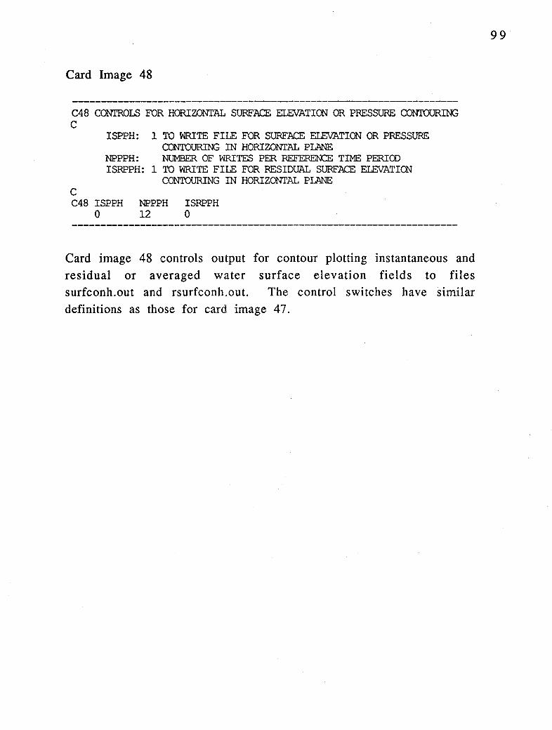
Card Image 48

C48 CONTROLS FOR HORIZONTAL SURFACE ELEVATION OR PRESSURE CONTOURING C

C

ISPPH: 1 TO WRI'IE FIIE FOR SURFACE ELEVATION OR PRESSURE CONTOURING IN HORIZONTAL PLANE

NPPPH: NUMBER OF WRITES PER REFERD.CE TIME PERIOO ISRPPH: 1 TO WRI'IE FIIE FOR RESIDUAL SURFACE ELEVA.TICN

CONTOURING IN HORIZONTAL PLANE

C48 ISPPH NPPPH ISRPPH 0 12 0

Card image 48 controls output for contour plotting instantaneous and residual or averaged water surface elevation fields to files surfconh.out and rsurfconh.out. The control switches have similar definitions as those for card image 47.

99

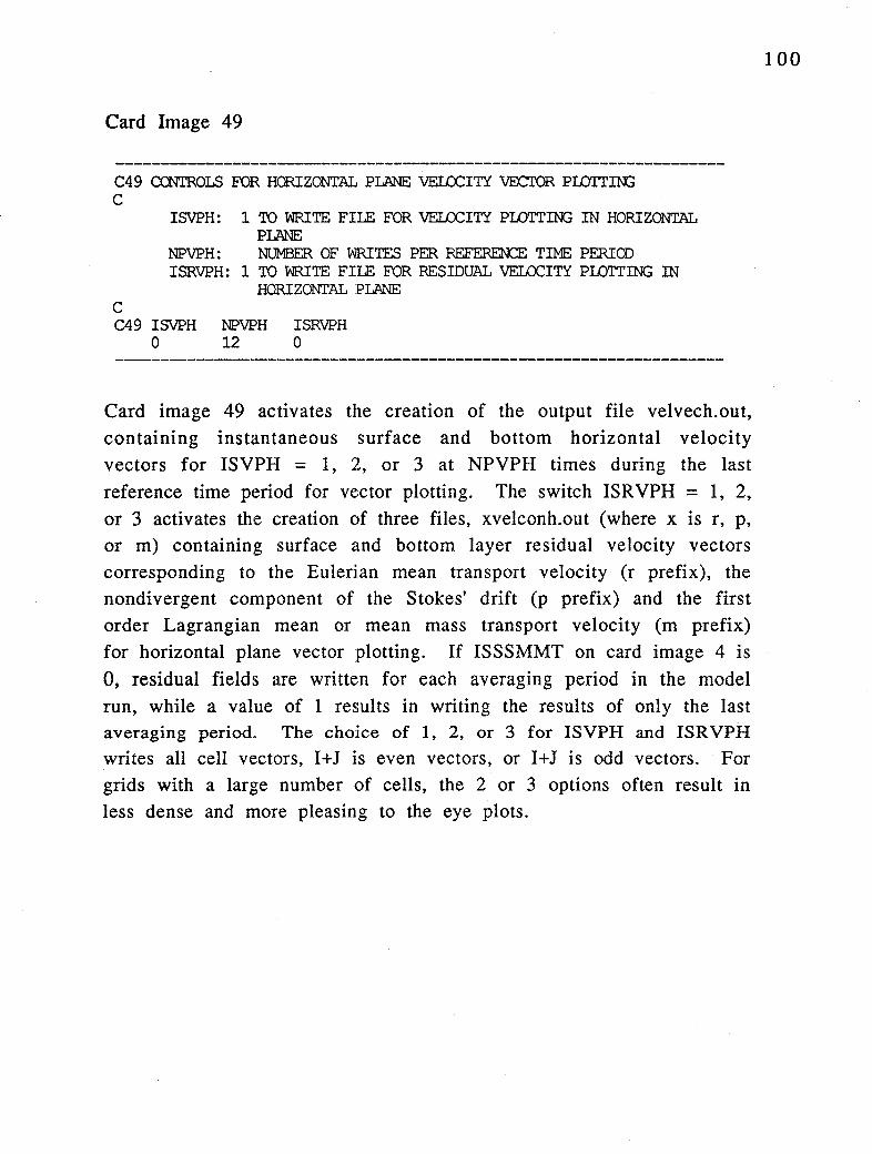
Card Image 49

C49 CCNI'ROLS FOR HORIZONTAL PLANE VELCCITY VECTOR PWTTING C

C

ISVPH: 1 TO WRITE FII.E FOR VELCCITY PI.OTTING IN HORIZONTAL PLANE

NPVPH: NUMBER OF WRITES PER REFEREN:E TIME PERICO ISRVPH: 1 TO WRI1:'E FII.E FOR RESIDUAL VELCCITY PWTTING IN

HORIZONTAL PLANE

C49 ISVPH NPVPH ISRVPH 0 12 0

Card image 49 activates the creation of the output file velvech.out,

containing instantaneous surface and bottom horizontal velocity

vectors for ISVPH = 1, 2, or 3 at NPVPH times during the last

reference time period for vector plotting. The switch ISRVPH = 1, 2,

or 3 activates the creation of three files, xvelconh.out (where x is r, p, or m) containing surface and bottom layer residual velocity vectors

corresponding to the Eulerian mean transport velocity (r prefix), the

nondivergent component of the Stokes' drift (p prefix) and the first

order Lagrangian mean or mean mass transport velocity (m prefix)

for horizontal plane vector plotting. If ISSSMMT on card image 4 is

0, residual fields a.re written for each averaging period in the model

run, while a value of l results in writing the results of only the last averaging period. The choice of 1, 2, or 3 for ISVPH and ISRVPH

writes all cell vectors, I+J is even vectors, or I+J is odd vectors. For

grids with a large number of cells, the 2 or 3 options often result in

less dense and more pleasing to the eye plots.

100

Card Image 50

CSO CONTROLS FOR VERTICAL PLANE SCALAR FIEID CONTOURING C

ISE.CSPV:

NPSPV: ISSPV: ISRSPV: ISHPLTV:

C CSO ISE.CSPV

2

AN INI'EGER NUMBER OF VERTICAL SECTIONS (N.IE. 99) TO WRI~E ISECSPV FIIES FOR SCALAR FIEID CONTOURJN:; NUMBER OF WRITES PER REFEREN::E TIME PERICD 1 TO ACTIVATE INSTANTANEOUS SCALAR FIEIDS 1 TO ACTIVATE FOR RESIDUAL SCALAR FIEIDS 1 FOR VERTICAL PLANE PI.OTTING FOR MSL DATUMS, ZERO OTHERWISE

NPSPV ISSPV ISRSPV ISHPLTV 12 1 1 1

Card image 50 activates output of information for vertical plane scalar field contouring for ISCESPV vertical sections or transects. The switch ISSPV activates output of instantaneous values NPSPV times during the last reference time period to the files xxxcnvN.out (xxx equals sal, tern, dye, scd, or sfl, and N represents the section number currently limited to a maximum of 9). The switch ISRSPV activates output of time-averaged or residual variables to similar r-prefixed files after each averaging period (ISSSMMT = 0) or only the last averaging period (ISSMMT = 1) with the time steps in the averaging period defined by NTSMMT on card image 7. The last parameter configures the plotting information for tidal or other datums. Additional information is specified on card images 51 and 52.

101

Card Image 51

CSl M:'RE CONTROLS r.""OR VERTICAL PLANE SCALAR FIE.ID CON'l'OURIN:; C

ISECSPV: SECTICN NUMBER NIJSPV: NUMBER OF CEIJ.S OR I,J PAIRS IN SECTION SEC ID: CHARACI'ER FORMAT SECTION TITLE

C CSl ISECSPV NIJSPV SEC ID

1 14 'JR BRIDG:' 2 10 'NN PT 45'

Card image 51 provides information to define the vertical plane transects. A line of data is required for each vertical section. The maximum number of vertical sections is currently limited to 9. The first parameter identifies the section number, the second parameter specifies the number of cells comprising the section, and the last character string provides an identifier which is also written to the output files.

102

Card Image 52

CS2 I,J I.OCATIONS FOR 'VERTICAL PLANE SCALAR FIEID CON'I'OURIN:; C

ISECSPV: SECTICN' NCJMBER ISPV: I CELL JSPV: J CELL

C CS2 ISECSPV ISPV JSPV

1 117 52 1 118 53 1 119 54 1 120 55 1 121 56 1 122 57 1 123 58 1 124 59 1 125 60 1 126 61 1 127 62 1 128 63 1 129 64 1 130 65 2 141 39 2 142 40 2 143 41 2 144 42 2 145 43 2 146 44 2 147 45 2 148 46 2 149 47 2 150 48

Card image 52 defines the sequence of cells comprising the section, with the first parameter being for user identification. The other two parameters define the section sequenced by I and J cell indices. It is noted that cells in the sequence do not need to be adjacent, nor do they need to follow a straight line. For example, they may represent instrument locations, longitudinal moving survey locations, or interesting cross sections of the flow field or a typical longitudinal section up an estuary.

103

Card Image 53

C53 CCNI'ROIS FOR VERTICAL PLANE VEI..OCITY VECTOR PLOTTm:; C

ISFDJPV:

NPVPV: ISVPV: ISRSPV:

C C53 ISFDJPV

2

AN INTEGER NUMBER (N. LE. 9) OF VERTICAL SECTIONS TO WRITE ISFDJPV FILES FOR VELOCITY PLOTTm:;

NUMBER OF WRITES PER REFEREN:E TIME PERICD 1 TO ACTIVATE INSTANTANEOUS VELOCITY 1 TO ACTIVATE FOR RESIDUAL VELOCITY

NPVPV ISVPV ISRSPV 12 0 1

Card image 53 activates output of information three types of vector plotting in ISECVPV (currently limited to 9) vertical planes. The switch ISVPV activates output of instantaneous data at NPVPV times during the reference time period, while ISRSPV activates output of time averaged or residual data after each averaging period (ISSSMMT = 0), defined by NTSMMT on card image 7, or the last averaging period (ISSSMMT = 1). The first class of output files provides data for plotting vectors tangential to the vertical plane. Instantaneous data are written to the files velvcvN.out, while residual data are written to the files rvelvcvN.out, pvelvcvN.out, mvelvcvN.out, lmvvcvN.out, and almvvcvN.out, where N indicates the second number. The last two files are written only if ISLRD is not zero. The second class of output files provides data for contour

plotting the component of the hodzontal velocity normal to the vertical planes. Instantaneous data are written to the files velcnvN.out, while residual data are written to the files rvelcnvN.out, pvelcnvN.out, mvelcnvN.out, lmvcnvN.out, and almvcnvN.out. The last two files are written only if ISLRD is not zero. The final class of output files provides data for contour plotting the component of the horizontal residual velocities tangential to the vertical plane. Timeaveraged or residual data are written to the files rvelcvtN.out, pvelcvtN.out, mvelcvtN.out, lmvcvtN.out, and almvcvtN.out, again with the last two files written to as ISLRD is not zero.

104

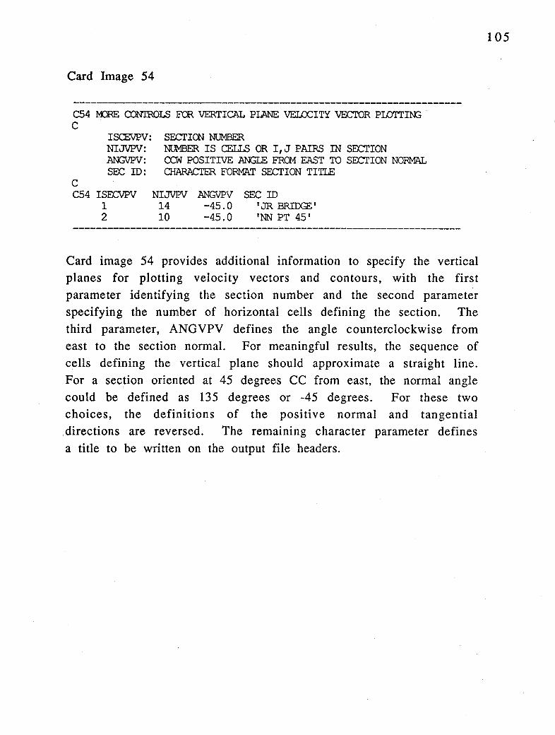
Card Image 54

C54 M)RE CONTROIS FOR VERTICAL PLANE VEUX:ITY VECTOR PLOTTIN:; C

C

ISCENPV: NIJVPV: lillGJPV: SEC ID:

C54 ISECVPV 1 2

SECTICN NUMBER NUMBER IS CEIJ:.S OR I, J PAIRS IN SECTION earl POSITIVE ANGLE FRCM EAST TO SECTION NORMAL CHARACTER FORMAT SECTION TITLE

NIJVPV AfJGVPV SEC ID 14 -45.0 'JR BRIDGE' 10 -45.0 'NN PT 45'

Card image 54 provides additional information to specify the vertical planes for plotting velocity vectors and contours, with the first parameter identifying the section number and the second parameter specifying the number of horizontal cells defining the section. The third parameter, ANGVPV defines the angle counterclockwise from east to the section normal. For meaningful results, the sequence of cells defining the vertical plane should approximate a straight line. For a section oriented at 45 degrees CC from east, the normal angle could be defined as 135 degrees or -45 degrees. For these two choices, the definitions of the positive normal and tangential . directions are reversed. The remaining character parameter defines a title to be written on the output file headers.

105

Card Image 55

C55 (X)NTR()I.S FOR VERTICAL PLANE VEI.OCITY PLOTTING C

ISECVPV: SECTION NUMBER (REFERENCE USE HERE) IVPV: I CELL INDEX JVPV: J CELL INDEX

C C55 ISECVPV IVPV JVPV

52 53 54 55 56 57 58 59 60 61 62 63 64 65 39 40 41 42 43 44 45 46 47 48

1 117 1 118 1 119 1 120 1 121 1 122 1 123 1 124 1 125 1 126 1 127 1 128 1 129 1 130 2 141 2 142 2 143 2 144 2 145 2 146 2 147 2 148 2 149 2 150

Card image 55 specifies the sequence of I and J indices defining the vertical plane sections.

106

Card Image 56

C56 CONTROL.5 FOR 3D FIE:I.D OUTPUT C

IS3D:

ISR3D:

NP3D:

KPC: NWGG:

I3DMI: I3DMA: J3DMI: J3DMA: J3RW: SEI.MX: BEIMN:

C .

1 TO WRITE: TO 3D ASCII INTEGER FORMAT FILES 2 TO WRITE: TO 3D OIARACTER ARRAY FORMAT FILES (NOT

ACTIVE) 3 TO WRIIB TO 3D HDF IMAGE FORMAT FIIBS (NOT ACTIVE) 4 TO WRIIB TO 3D HDF FLOATING POINT FORMAT FILES (NOT ACTIVE) (IS3D IS IS300 IN CODE) SAME AS IS300 EXCEPT FOR RESIDUAL VARIABLES (ISR3D IS ISR300 IN CODE)

NUMBER OF WRITES PER LAST REF TIME PERIOD FOR INST VARIABLES (NP3D IS NP300 IN CODE) NUMBER OF UNS'I'RETOill) PHYSICAL VERTICAL LAYERS NUMBER OF WAIBR CELLS IN CARTESIAN 3D GRAPHICS GRID OVERIAY OF A CURVILINEAR GRID. FOR EFOC RUNS ON A CURVILINEAR GRID, I3DMI,I3DMA,J3DMI,J3DMA REFER TO CELL INDICES ON THE ON THE CARTESIAN GRAPHICS GRID OVERI.AY DEFINED BY FILE gcell.inp. THE FILE gcell.inp IS IDT USED BY EFOC, BUT BY THE COMPANION GRID GENERATION CODE GEFDC.F. INFORMATION DEFINING THE OVERIAY IS READ BY EFDC.FOR FROM FILE gcellmap.inp MINIMJM OR BEGINNIN:; I INDEX FOR 30 ARRAY OUTPUT MAXIMJM OR ENDING I INDEX FOR 3D ARRAY OUTPUT MINIMJM OR BEGINNIN:; J INDEX FOR 30 ARRAY OUTPUT MAXIMJM OR ENDING J INDEX FOR 30 ARRAY OUTPUT

1 REWRITE F'IIF...S TO CORRECT ORIENTATION MAXIMJM SURFACE ELEVATION FOR UNSTRETCHIN:; MINIMUM BOTTOM ELEVATION FOR UNSTRETCHIN;

C56 IS3D ISR3D NP3D KPC NWGG I3DMI I3DMA J3DMI J3DMA I3DRW SEI.MX BEI.MN 0 0 6 1 0 2 3 2 3 1 4.0 -32.0

Card image 56 controls the output of three-dimensional data for graphics and visualization. The switches IS3D and ISR3D activate output of instantaneous data at NP3D times during the last reference time period and time averaged or residual data respectively. The residual data is output after each averaging period (ISSSMMT = 0), defined by NTSMMT on card image 7, or only the last averaging period (ISSMMT = 1). However the current configuration allows only 24 averaged output files, and if the number of averaging periods for a run exceeds 24, only the last 24 periods are output. The only currently active option (IS3D==l and ISR3D=l) writes output as eight

107

bit ASCII integers (0 to 255). This choice was made for flexibility and the minimization of disk storage. A post processor is available via ftp to translate the 8 bit ASCII integer data to a number of alternate forms including 8 bit ASCII character data, 8 bit binary, and HDF image or floating point format for compatibility with various visualization software. Although the 8 bit three-dimensional integer array files may be very large, they can be efficiently compressed on most systems. On UNIX systems, the UNIX .Z compressed version of the output files may be up to a factor 10 times smaller.

The output format is a three-dimensional array which can be conceptualized as a stack of KPC layers, of equal thickness, which slice the model domain at constant elevation plane, progressing from above the maximum water surface elevation to below the minimum bottom elevation. Each layer (or plane) comprises a two-dimensional array with a true east-north alignment. The most rapid variation in the two-dimensional plane is from west to east analogous to the columns of a spread sheet. The sequence of columns is written from north to south analogous to the rows of a spread sheet. Thus if a layer of the 3 matrix is viewed in a spread sheet type form, it will have the proper geographic orientation. The KPC constant elevation slices are generated by constant elevation interpolation equivalent to

an unstretching of the model's internal stretched or sigma coordinate system. The upper bounding elevation of the first layer is specified by elevation SELMX, which should be slightly larger than the maximum water surface elevation during the entire data sampling period. The lower bounding elevation of the last layer is specified by BELMN, which should correspond to an elevation slightly below the bottom of the deepest cell in the model domain. The values SELMX and BELMN shown in the example data line above are referenced to a sea level datum, hence the negative value of BELMN. For constant spacing Cartesian grids, the rectangular two-dimensional arrays or matrices corresponding to the constant elevation layers directly coincide with the model grid.

108

For curvilinear, or variable--spacing, Cartesian grids, a Cartesian graphics grid overlay, which can be generated by the preprocessor code GEFDC, and is input into EFDC by the file gcellmap.inp and is used to define the horizontal layers. The parameter NWGG defines the number of water cells in the Cartesian graphic grid. If NWGG is zero, the computation grid is assumed to be Cartesian, while a nonzero value indicates an overlay and activates the reading of the file gcellmap.inp. The input: file gcellmap.inp includes information from interpolating the curvilinear grid data to the Cartesian graphic grid. The extent of the horizontal region over which threedimensional data is to be extracted is defined by 13DMl<IG< 13DMA, and J3DMl<JG< J3DMA, where JG and JG are east and north indices in the Cartesian graphics grid overlay or the I and J indices of an equal spacing Cartesian computational grid. The parameter 13DRW allows the three-dimensional output to be written 1n a temporary compressed form. If 13DRW is set to 1, the output files are in the three-dimensional array structure described above. However, from many model applications to irregular regions, a large percent of the three-dimensional output matrix represents dry land. Setting 13DRW to zero results in output of information for active water cells in either the graphics overlay or computation grid. This output can later be expanded into the aforementioned fully three-dimensional format by a post processing utility, available via ftp.

109

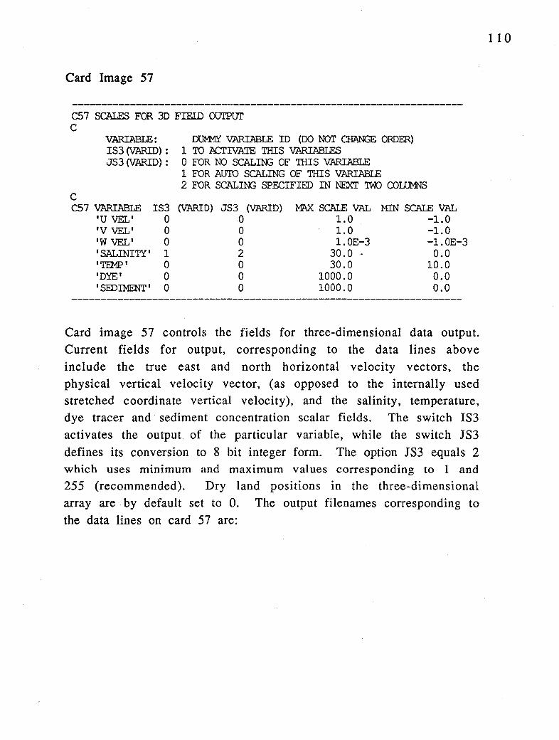
Card Image 57

C57 SCALES FOR 3D FIEID OUTPUT C

VARIABLE: DUM1Y VARIABLE ID (DO NOT CHANGE ORDER) IS3 (VARIO) : 1 TO ACTIVATE THIS VARIABIES JS3 (VARID): 0 FOR NO SCALING OF THIS VARIABLE

1 FOR .AUTO SCALING OF THIS VARIABLE 2 FOR SCALING SPECIFIED IN NF.JCT TWO COLUMNS

C C57 VARIABLE IS3 (VARID) JS3 (VARIO) MAX SC.ALE VAL MIN SCALE VAL

'U VEL' 0 0 1.0 -1.0 'V VEL' 0 0 1. 0 -1.0 'W VEL' 0 0 l.OE-3 -1.0E-3 'SALINITY' 1 2 30.0 • 0.0 'TEMP' 0 0 30.0 10.0 'DYE' 0 0 1000.0 0.0 'SEDIMENT' 0 0 1000.0 0.0

Card image 57 controls the fields for three-dimensional data output. Current fields for output, corresponding to the data lines above include the true east and north horizontal velocity vectors, the physical vertical velocity vector, (as opposed to the internally used stretched coordinate vertical velocity), and the salinity, temperature, dye tracer and sediment concentration scalar fields. The switch IS3 activates the output. of the particular variable, while the switch JS3 defines its conversion to 8 bit integer form. The option JS3 equals 2 which uses minimum and maximum values corresponding to 1 and

255 (recommended). Dry land positions in the three-dimensional array are by default set to 0. The output filenames corresponding to the data lines on card 57 are:

110

Output Variable Instantaneous Residual

UVEL uuu3dNN.asc ruuu3dNN.asc

VVEL vvv3dNN .asc rvvv3dNN .asc

WVEL www3dNN.asc rwww3dNN .asc

SALINITY sal3dNN .asc rsal3dNN.asc

TEMP tem3dNN.asc rtem3dNN.asc

DYE dye3dNN .asc rdye3dNN .asc

SEDIMENT sed3dNN.asc rsed3dNN .asc

where NN represents a two digit time sequence identified between 1 and 24. Two additional files, out3d.dia and rout3d.dia, provide summary information including the actual minimum and maximum values of each variable for the output files.

Card Image 5 8

C58 CONTROLS FOR WRITING TO TIME SERIES FIIES C

C

IS'IMSR: 1 OR 2 TO WRITE TIME SERIES OF SURF EIEV, VELCCITY, NET INI'ERNAL AND EXTERNAL MJDE VOLUME SOURCE-SINKS, AND COOCENTRATION VARIABIES, 2 APPENDS EXISTING TIME SERIES FIIES

:ML1MSR: NUMBER OF HORIZONTAL LOCATIONS TO WRITE TIME SERIES OF SURF EIEV, VELCCITY, AND CONCENTRATION VARIABIES, (MAXIMUM LOCATIONS = 99)

NB'IMSR: TIME STEP TO BEGIN WRITING TO TIME SERIES FIIBS NS'IMSR: TIME STEP TO STOP WRITING TO TIME SERIES FIIBS NWI'SER: WRITE INTERVAL FOR WRITING TO TIME SERIES FIIBS TCTMSR: UNIT CONVERSION FOR TIME SERIES TIME. FOR SECONDS,

MINUTES, HOURS,DAYS USE 1.0, 60.0, 3600.0, 86400.0 RESPECTIVELY

C58 IS'IMSR :MLTMSR NBTMSR NS'IMSR NWTMSR TC'IMSR 1 3 1 32000 36 3600.

1 1 1

Card image 58 activates and controls the writing of time series files. The parameter ISTMSR = 1 activates the creation of new time series files, while ISTMSR = 2 writes to the end of existing time series files and is useful in certain cases where the model is restarted to continue a long simulation. Instantaneous data for various model variables may be output at MLTMSR locations (the current limit is 99 locations). The parameters NBTMSR and NSTMSR specify the beginning and ending time steps of a time interval where data is output at every NWTMSR time steps. The conversion factor TCTMSR specifies the time units for the time column in the time series output files.

Card Image: 59

C59 CONTROLS FOR WRITING TO TIME SERIES FILES C

ILTS: JLTS: MI'SP: MI'SC: MI'SA: MI'SUE: MI'SUr: MI'SU: MI'SQE: MI'SQ: CLTS:

C C59 ILTS JLTS

128 62 125 59 123 58

I CELL INDEX J CELL INDEX

1 FOR TIME SERIES OF SURFACE ELEVATION 1 FOR TIME SERIES OF TRANSPORTED CONCENTRATION VARIABLES 1 FOR TIME SERIES OF EDDY VISCOSITY AND DIFFUSIVITY 1 FOR TIME SERIES OF EXTERNAL MODE HORIZONTAL VELCCITY 1 FOR TIME SERIES OF EXTERNAL MODE HORIZONTAL TRANSPORT 1 FOR TIME SERIE·s OF HORIZONTAL VELCCITY IN EVERY IAYER 1 FOR TIME SERIES OF NET EXTERNAL MODE VOLUME SOURCE/SINK 1 FOR TIME SERIES OF NET EXTERNAL MODE VOUJME SOURCE/SINK

:u:x:ATION AS A OIARACTER VARIABLE

MI'SP MI'SC MI'SA MI'SUE MI'SUT MI'SU MI'SQE MI'SQ 1 1 1 1 1 1 1 1 1 1 1 1 1 1 1 1 1 1 1 1 1 1 1 1

CLTS 'JRB A' 'JRB B' 'JRB C'

Card image 59 specifies the I and J indices of horizontal locations for writing time series data and the class of data. The generic file names created by the activation of the output switches are:

112

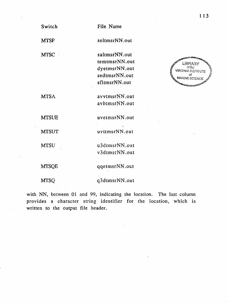
Switch

MTSP

MTSC

MTSA

MTSUE

MTSUT

MTSU

MTSQE

MTSQ

File Name

seltmsrNN.out

saltmsrNN .out temtmsrNN .out dyetmsrNN .out sedtmsrNN .out sfltmsrNN .out

avvtmsrNN .out avbtmsrNN .out

uvetmsrNN .out

uvttmsrNN.out

u3dtmsrNN .out v3dtmsrNN.out

qqetmsrNN .out

q3dtmsrNN.out

with NN, between 01 and 99, indicating the location. The last column provides a character string identifier for the location, which is written to the output file header.

113

Card Image 60

C60 CONTROLS FOR EXTRAC'TING INSTANTANEOUS VERT SCALAR FIEID PROFILES C

ISVSFP: MDVSFP: MLVSFP:

TMVSFP: TAVSFP:

C

1 FOR EX'l'RACTING INSTANTANEOUS VERTICAL FIEID PROFILES MAXIMUM NUMBER OF DEPTHS FOR SAMPLING VAUJE.5 NUMBER OE' HORIZONTAL SPACE-TIME LOCATION PAIRS TO BE SAMPIED MULTIPLIER 'TO CONVERT SAMPLING TIMES TO SECONDS ADDITIVE ADJUS'IMENT TO SAMPLING TIME BEFORE (X)NVERSION TO SEC

C60 ISVSFP M)VSFP MLVSFP TMVSFP TAVSFP 1 8 10 3600. 0.0

Card image, 60 provides for the extraction of instantaneous vertical scalar field profiles at specified times an locations. This option is designed to mimic field sampling surveys and produce a smaller volume of output data than the time series output option. The switch ISVSFP = 1 activates the option. The parameter MDVSFP specifies the maximum number of depths (measured downward from the instantaneous free surface for sampling, while ML VSFP specifies the number of discrete time and space locations for sampling. The parameter TMVSFP converts the sampling times specified on card image 62 to seconds. The time origin for specifying sampling should be consistent with information specified on card image 8. The parameter TA VSFP is an additive adjustment to the sampling times on card image 63, and is useful for dealing with sampling times recorded during daylight savings conditions. Output for this option is written to the file vsfp.out.

114

Card Image 61

C61 SAMPLING DEPTHS FOR E.xTRACTING INST VERT Sc.ALAR FIEID PROFILES C

M1DVSFP: Mth SAMPLING DEPTH DMSFP: SAMPLING DEPTH BELOW SURFACE, IN METERS

C C61 M1DVSFP

1 2 3 4 5 6 7 8

DMVSFP 1.0 3.0 5.0 7.0 9.0

11.0 13.0 15.0

Card image: 61 specifies the MDVSFP sampling depths below the water surface at the specified times and locations. If the local depth to the bottom is less than a sample depth, output data is not written for that depth.

115

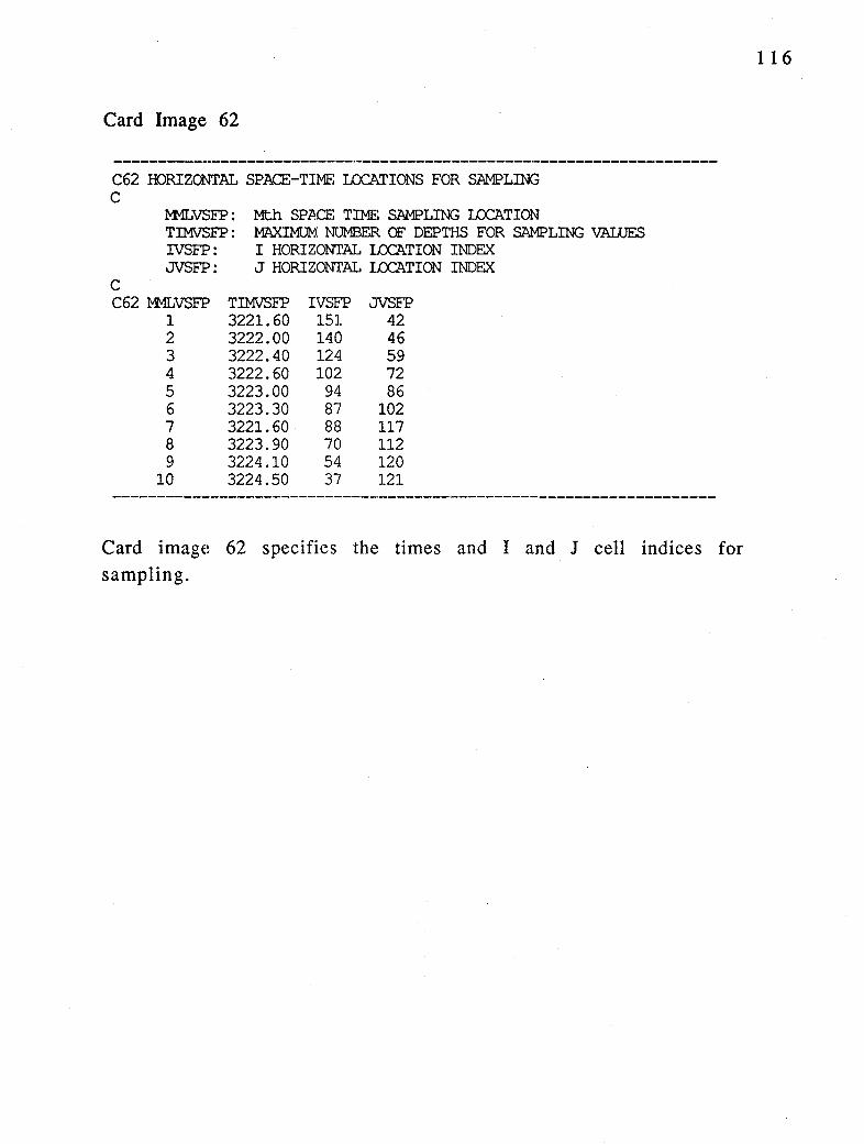
Card Image 62

C62 HORIZONTAL SPACE-TIME: I..CX::'ATIONS FOR SAMPLING C

1:-MLVSFP: TIMVSFP: IVSFP: JVSFP:

C

Mth SPACE: TIME: SAMPLING ux::ATION MAXIMUM: NUMBER OF DEPTHS FOR SAMPLING VALUES I HORIZONTAL IAAATION INDEX J HORIZONTAL IAAATION INDEX

C62 M1LVSFP TIMVSFP IVSFP JVSFP 1 3221.60 151 42 2 3222.00 140 46 3 3222.40 124 59 4 3222.60 102 72 5 3223.00 94 86 6 3223.30 87 102 7 3221.60 88 117 8 3223.90 70 112 9 3224.10 54 120

10 3224.50 37 121

Card image 62 specifies the times and I and J cell indices for sampling.

116

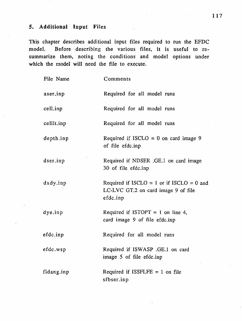
5. Additional Input FHes

This chapter describes additional input files required to run the EFDC model. Before describing the various files, it is useful to resummarize them, noting the conditions and model options under which the model will need the file to execute.

File Name

aser.inp

cell.inp

celllt.inp

depth.inp

dser.inp

dxdy.inp

dye.inp

efdc.inp

efdc.wsp

fldang.inp

Comments

Required for all model runs



Required if ISCLO = 0 on card image 9 of file efdc.inp

Required if NOSER .GE.I on card image 30 of file efdc.inp

Required if ISCLO = I or if ISCLO = 0 and LC-LVC GT.2 on card image 9 of file efdc.inp

Required if ISTOPT = 1 on line 4, card image 9 of file efdc.inp


Required if ISW ASP .GE. I on card image 5 of file efdc.inp

Required if ISSFLFE = I on file sfbser.inp

117

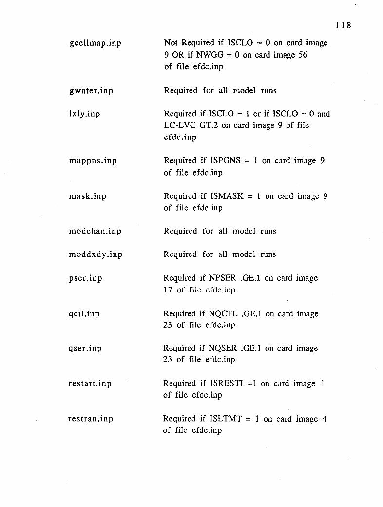
gcellmap.inp

gwater.inp

lxly.inp

mappns.inp

mask..inp

modchan.inp

moddxdy .inp

pser.inp

qctl.inp

qser.inp

restart.inp

restra.n .inp

Not Required if IS CLO = 0 on card image 9 OR if NWGG = 0 on card image 56 of file efdc.inp


Required if ISCLO = 1 or if ISCLO = 0 and LC-LVC GT.2 on card image 9 of file efdc.inp

Required if ISPGNS = 1 on card image 9 of file efdc.inp

Required if ISMASK = 1 on card image 9 of file efdc.inp



Required if NPSER .GE.l on card image 17 of file ef dc.inp

Required if NQCTL .GE. I on card image 23 of file efdc.inp

Required if NQSER .GE.1 on card image 23 of file efdc.inp

Required if IS RES TI = 1 on card image 1 of file ef dc.inp

Required if ISL TMT = 1 on card image 4 of file efdc.inp

118

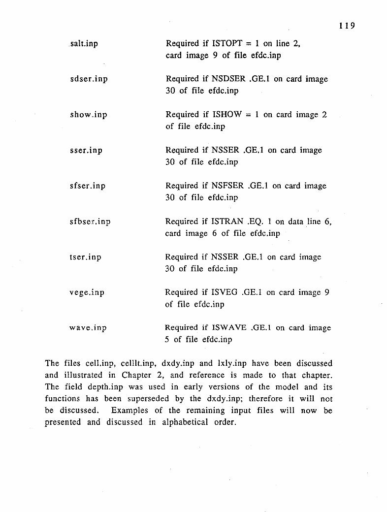
salt.inp

sdser.inp

show..inp

sser.inp

sfser .inp

sfbser.inp

tser .inp

vege.inp

wave.inp

Required if ISTOPT = 1 on line 2, card image 9 of file efdc.inp

Required if NSDSER .GE.I on card image 30 of file efdc.inp

Required if ISHOW = 1 on card image 2 of file efdc.inp

Required if NSSER .GE.I on card image 30 of file ef dc.inp

Required if NSFSER .GE. I on card image 30 of file efdc.inp

Required if ISTRAN .EQ. I on data line 6, card image 6 of file ef dc.inp

Required if NSSER .GE. I on card image 30 of file efdc.inp

Required if ISVEG .GE. I on card image 9 of file efdc.inp

Required if ISW A VE .GE.1 on card image 5 of file efdc.inp

The files cell.inp, celllt.inp, dxdy.inp and lxly.inp have been discussed and illustrated in Chapter 2, and reference is made to that chapter. The field depth.inp was used in early versions of the model and its functions has been superseded by the dxdy .inp; therefore it will not be discussed. Examples of the remaining input files will now be presented and discussed in alphabetical order.

119

Input file aser.inp

The input file aser.inp specifies atmospheric, wind and thermal f orcings as well as precipitation and evapotranspiration. For ISTOPT = 1 on line 3 of card image 6, the full set of environmental parameters for an internal-to-the-model calculation of thermal sources and sinks is specified in the file. An example of the aser.inp file for this case is:

C aser.inp file, in free format across line, repeats naser=l times C C MASER 'rCASER TAASER WINDSCT RAINCVT EVAPCVT C C TASER WINDS WINDD PATM TDRY TWET RAIN EVAP SOLSWR C

4 86400. 0.0 1.0 1.0 1.0 73.46 4.13 161. 1000. 25. 20. . 28E-08 .29E-07 500 . 73.50 3.96 148. 1000. 25. 20. . OOE+OO .29E-07 500 . 73.54 4.25 144. 1000. 25. 20. . 56E-08 .29E-07 500 . 73.58 3.82 132. 1000. 25. 20. . 17E-07 .29E-07 500 .

Parameters on the first data line specify the number of time points (MASER), a factor to convert the time units to seconds (TCASER), a constant time to be added before unit conversion (T AASER), a factor to convert wind speed to meters/second (WINDSCT), and factors to convert rainfall and evapotranspiration rates to meters per second (RAINCVT., EVAPCVT). Each time lines data has in order: time (TASER), wind speed (WINDS), wind direction (WINDD) in bearing angle to the direction the wind is blowing ( oceanographic as opposed

to meteorological convention), atmospheric pressure (PATM) in millibars, dry and wet bulb temperature (TORY, TWET) in degrees C, rainfall rate (RAIN), evapotranspiration rate (EV AP) and incident solar short-wave radiation (SOLSWR) in Joules per seconds per square meter. For ISTOPT = 2 on line 3 of card image 6, a time variable equilibrium temperature surface heat exchange formulation is implemented in the model. The form of the aser.inp file for this case is identical to that above, except that now the equilibrium temperature (degrees C) is entered under the TORY column and the net surface heat exchange coefficient in square meters per second is entered under the SOLSWR column. Data entered under PATM and

120

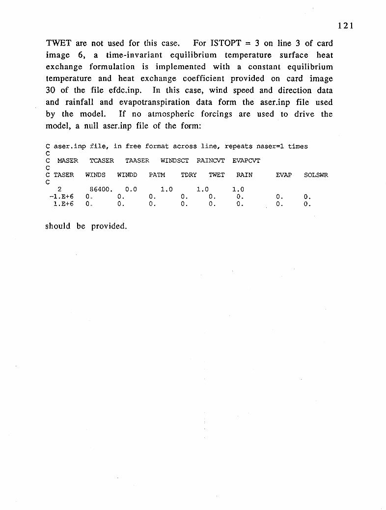
TWET are not used for this case. For ISTOPT = 3 on line 3 of card image 6, a time-invariant equilibrium temperature surface heat exchange formulation is implemented with a constant equilibrium temperature and heat exchange coefficient provided on card image 30 of the file ef dc.inp. In this case, wind speed and direction data and rainfall and evapotranspiration data form the aser.inp file used by the model. If no atmospheric forcings are used to drive the

model, a null aser.inp file of the form:

C aser.inp file, in free format across line, repeats naser=l times C C MASER TCASER TAASER WINDSCT RAINCVT EVAPCVT C C TASER WINDS WINDD PATM TDRY TWET RAIN EVAP SOLSWR C

2 -1.E+6

1.E+6

86400. 0 .. 0 ..

0.0 o. 0.

should be provided.

0. 0.

1. 0 o. 0.

1.0 o. 0.

1.0 0. 0.

0. 0.

0. 0.

121

122

Input filles dser.inp, sser.inp, sdser.inp, sfser.inp, and tser.inp

The scalar constituent time series files have identical formats, and thus it suffices to discuss them in a generic sense. An example of the sser.inp time series file containing one time seties is shown below.

c sser. inp file, salt i.s nc=l cone, in free format across line, C repeats ncser(l).times, test case C C ISTYP MCSER(NS,l) TCCSER(NS,l) TACSER(NS,1) RMULADJ(NS,l) ADDADJ(NS,l) C C if istyp.E~q.1 then read depth weights and single value of CSER C C (WKQ (K), K==l, KC) C C TCSER(M,NS,l) CSER(M,NS,l) ! (mcser(ns,l) sets ns=l,ncser(l) series) C C else read a value of qser for each layer C C TCSER(M,NS,l) (CSER(M,K,NS,l),K=l,KC) ! (mcser(ns,l) pairs) C

0 7 86400. 0.0 1. 0 0.0 35.791668 29.57 29.57 29.57 29.57 29.57 29.57 29.57 35.833336 29.93 29.93 29.93 29.93 29.93 29.93 29.93 35.875000 29.88 29.88 29.88 29.88 29.88 29.88 29.88 35.916668 30.89 30.89 30.89 30.89 30.89 30.89 30.89 35.958336 31.24 31.24 31. 24 31.24 31.24 31.24 31.24 36.000000 31.12 31.12 31.12 31.12 31.12 31.12 31.12 36.041668 31.28 31.28 31.28 31.28 31.28 31.28 31.28

29.57 29.93 29.88 30.89 31.24 31.12 31.28

A concentration time series input file may contain multiple time series. Each time series set begins with the single data line specifying ISTYP (the time series format identifier), MCSER (the number of time data points), TCCSER (a multiplying conversion factor changing the input time units to seconds), TACSER (an additive time adjustment, applied before unit conversion), RMULADJ (a multiplying conversion for the concentration), and ADDADJ (an additive conversion for concentration, applied before the multiplier). If the ISTYP parameter is 0, the MCSER time data points must have a concentration value for each layer. If ISTYP is 1, an additional line of

data providing interpolating factors is read, and the time data lines

should have only one concentration value. ISTYP=l dser.inp file is shown below:

An example of an

C dser.inp file, dye is nc=3 cone, in free format across line, C repeats ncser(3) times, test case C C ISTYP MCSER(NS,3) TCCSER(NS,3) TACSER(NS,3) RMULADJ(NS,3) ADDADJ(NS,3) C C if istyp.eq.l then read depth weights and single value of CSER C C (WKQ (K), K==l, KC) C C TCSER(M,NS,3) CSER(M,NS,3) ! (rncser(ns,3) sets ns=3,ncser(3) serseries) C C else read a value of dser for each layer C C TCSER(M,NS,3) (CSER(M,K,NS,3),K=l,KC) ! (rncser(ns,3) pairs) C

1 10 0.0

-2000.0000 713.39 713. 41 726.89 726. 91

7076.49 7076.51 7087.99 7088.01 10000.00

3600.0 o. 0.00 0.00 0.00

0.00 0.00

2263374.5 2263374.5

0.00 0.00

2657004.85 2657004.85

0.00 0.00

1. 0. 0. 00 1. 00

This example specifies 6 weights (for a 6 layer model) on the second data line, which is read when ISTYP=l. The weights are read from the bottom to the top layer. For the example shown above, the dye is being released into the surface layer. (see the qser.inp file for the corresponding dye release flow rate formulation).

123

Input files dye.inp and salt.inp

The input files dye.inp and salt.inp are used to initialize the dye and salinity fields for cold start runs if an appropriate ISTOPT switch is set on card image 6 of the ef dc.inp file. An example of a portion of the salt.inp field is shown below.

C salt.inp :file, in freei format across line, for IRLTC Final Grid C first data line ISALTYP =Ono L,I,J =1 read L,I,J C L=2,LA rows of SALINIT(L,K),K=l,KC across columns C

1 1 40 2 30.62 30.62 30.62 30.62 30.62 30.62 30.62 2 41 2 30.62 30.62 30.62 30.62 30.62 30.62 30.62 3 42 2 30.62 30.62 30.62 30.62 30.62 30.62 30.62 4 43 2 30.62 30.62 30.62 30.62 30.62 30.62 30.62 5 40 3 0.0 0.0 0.0 0.0 o.o 0.0 0.0 6 41 3 0.0 0.0 0.0 0.0 0.0 0.0 0.0 7 42 3 0.0 0.0 0.0 0.0 0.0 0.0 0.0 8 43 3 0.0 0.0 0.0 0.0 0.0 0.0 0.0

30.62 30.62 30.62 30.62 0.0 0.0 0.0 0.0

The file has four header lines, followed by a line specifying the format type switch, ISALTYP. If ISALTYP is equal to I, LC-2 data lines follow in the order L=2,LA, which is the single index sequence of active water cells. For ISALTYP=l, the first three columns give L (the single horizontal internal cell index), and I and J (the two external indices). These are then followed by KC (the number of model layers) values of salinity read from the bottom to the surface.

For ISALTYP=O, the L, I, and J indices are absent from the data lines. A template for the salt.inp file, of !SAL TYP= 1 form, is generated by

GEFDC. However, the four header lines and ISALTYP=l must be manually added. The ISAL TYP=O format is carried over from older versions of the model. To allow conversion from older versions, the EFDC model outputs a file, newsalt.inp, of the ISAL TYP= 1, form.

124

Input file efdc. wsp

The file efdc.wsp provides data for controlling the linkage of EFDC and the WASPS series of water quality models (Ambrose, et. al. 1993) writing WASP format input files specifying cell volumes, flow and diffusion linkages and flow files in either generic or DYNHYD format. An example of the efdc.wsp input file is shown below.

Cl Cl

C2 C2

C3 C3

C4 C4

CELL VOLUME PARAMETERS for WASP-EFOC Linkage IVOPT IEDEV SC.ALV CONN VMULT VEXP DMULT DEXP 2 0 1.0 1.0 1.0 0. 1.0 o. DIFFUSION AND DISPERSION PARAMETERS NRFID SCAlR CONVR ISNKH 2 1.0 1.0 1 ADVECrION PARAMETERS (iqopt=3 ASCII HYD, IQOPT NFIEID SCALQ CONVQ HYDFIL 3 5 1.0 1.0 'NORWAI.K.HYD' DEPTH OF SEDIMENT LAYER (METERS) DEPSED TDINTS SEDIFF WSSl 0.1 366 2.315E-09 0.05

=4 for binary HYD file) ISWASPD ISDHD 0 0

WSS2 0.10

WSS3 0.15

The parame:ters on card images 1 and 2 are identical to those defined in the WASP user's manuals. Card images 3 and 4 provide information. for the flow and diffusive transport fields and the sediment submodel. EFDC users considering activating the WASP linkage option should contact the author for further information and guidance.

125

Input fih~ fldang.inp

The file fldang.inp is used to specify the direction of tidal flood flow and is used in shellfish larvae transport simulations (see file sfbser.inp) to cue larvae swimming behavior. It is a headerless file with LC-2 lines of data. The first few lines of an example are shown below.

98 3 131.46 133.67 99 3 166.15 165.82

100 3 173.50 175.51 101 3 210.48 211.48

96 4 148.08 144.86 97 4 166.50 161.98 98 4 149.75 145.43 99 4 169.05 167.36

The data on each line correspond to the I and J horizontal cell indices, followed by a bottom and surface layer flood direction angle. The angles, measured counter clockwise (CCW) from east specify the maximum tidal flood flow direction determined by an analysis of bottom and surface layer tidal velocity ellipses for a single dominant tidal constituent (usually M2 on the U. S. east coast). Tidal ellipse directions are obtained from the output files tidelkb.out and tidelkc.out generated by a preliminary model run. Contact the author for software to generate the fldang.inp file from the tidelkb.out and tidelkc.out files.

126

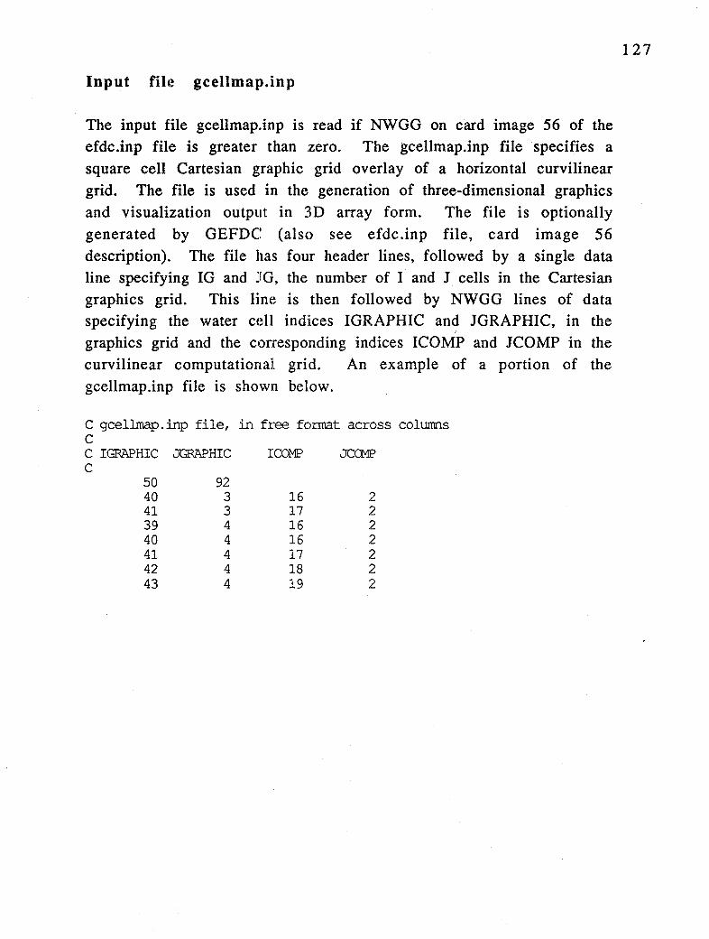
Input file gcellma1>.inp

The input file gcellmap.inp is read if NWGG on card image 56 of the efdc.inp file is greater than zero. The gcellmap.inp file specifies a square cell Cartesian graphic grid overlay of a horizontal curvilinear grid. The file is used in the generation of three-dimensional graphics and visualization output in 3D array form. The file is optionally generated by GEFDC (also see efdc.inp file, card image 56 description).. The file has four header lines, followed by a single data line specifying IG and JfG, the number of I and J cells in the Cartesian graphics grid. This line is then followed by NWGG lines of data specifying the water cell indices !GRAPHIC and JGRAPHIC, in the graphics grid and the corresponding indices ICOMP and JCOMP in the curvilinear computational grid. An example of a portion of the gcellmap.inp file is shown below.

C gcellmap.inp file, in free format across colurms C C IGRAPHIC JGRAPHIC ICCMP JCCMP C

50 40 41 39 40 41 42 43

92 3 3 4 4 4 4 4

16 17 16 16 17 18 19

2 2 2 2 2 2 2

127

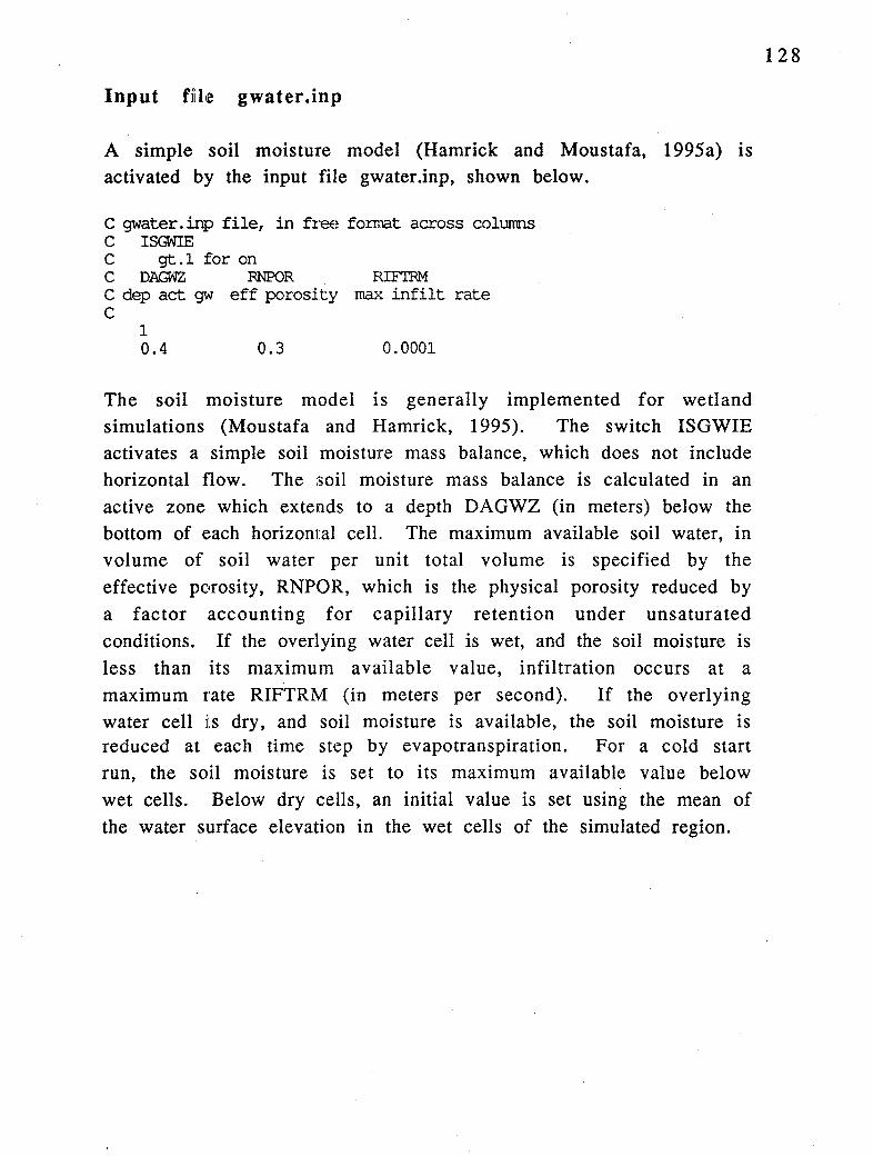
Input file gwater .inp

A simple soil moisture model (Hamrick and Moustafa, 1995a) is activated by the input file gwater.inp, shown below.

C gwater. inp file, in freE~ format across colUims C ISGWIE C gt.l for on C DAGWZ RNPOR RIFTRM C dep act gw eff porosity max infilt rate C

1 0.4 0.3 0.0001

The soil moisture model is generally implemented for wetland simulations (Moustafa and Hamrick, 1995). The switch ISGWIE activates a simple soil moisture mass balance, which does not include horizontal flow. The soil moisture mass balance is calculated in an active zone which extends to a depth DAGWZ (in meters) below the bottom of e:ach horizontal cell. The maximum available soil water, in volume of soil water per unit total volume is specified by the effective porosity, RNPOR, which is the physical porosity reduced by a factor accounting for capillary retention under unsaturated conditions. If the overlying water cell is wet, and the soil moisture is less than its maximum available value, infiltration occurs at a maximum rate RIFTRM (in meters per second). If the overlying water cell ils dry, and soil moisture is available, the soil moisture is reduced at each time step by evapotranspiration. For a cold start run, the soil moisture is set to its maximum available value below wet cells. Below dry cells, an initial value is set using the mean of the water surface elevation in the wet cells of the simulated region.

128

Input file mappgns.inp

The input file mappgns.inp is used to configure the EFDC model for the simulations of regions presumed to be periodic or infinite in the computational y or north-south direction, the prime example being an infinite continental shelf or nearshore region, or the same region under the assumption of spatially periodic forcing. An example of a portion of the file is shown below.

C ISPNS,JSPNS = I,J IIDICES OF A SOUTH CELL C INPNS,JNPNS = I,J IIDICES OF A CORRESPONDING NORTH CELL C NPNSBP C ISPNS JSPNS INPNS -.1NPNS {REPEATED NPNSBP TIMES) C

4 2 3 4 5

2 2 2 2

2 3 4 5

126 126 126 126

The parameter NPNSBP specifies the number of north-south pairs. This is followed by NPNSBP pairs of south and north I and J indices. North and south open boundary conditions must not be specified for these cell pairs in the ef dc.inp files.

129

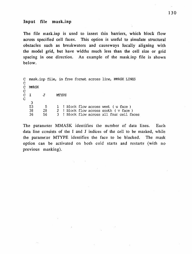
Input file mask.inp

The file mask.inp is used to insert thin barriers, which block flow across specified cell faces. This option is useful to simulate structural obstacles such as breakwaters and causeways locally aligning with the model grid, but have widths much less than the cell size or grid spacing in one direction. An example of the mask.inp file is shown below.

C mask. inp file, in free format across line, M-1ASK LINES C C M-1ASK C C I J MI'YPE C

3 53 c-

,) 1 Block flow across west ( u face ) 38 28 2 Block flow across south ( v face ) 36 56 3 Block flow across all four cell faces

The parameter MMASK identifies the number of data lines. Each data line consists of the I and J indices of the cell to be masked, while the parameter MTYPE identifies the face to be blocked. The mask option can be activated on both cold starts and restarts· (with no previous masking).

130

Input fil«~ modchan.inp

The input file modchan.inp is used to activate and specify data for a subgrid scale channel model. The subgrid scale channel model (Hamrick and Moustafa, 1995a,b; Moustafa and Hamrick, 1995) allows narrow, one-dimensional in the horizontal plane, channels to pass through larger scale, two-dimensional in the horizontal, cells, referred to as host cells. Up to two subgrid channels at arbitrary orientations may pass through a host cell. The two channels are referred to as u and v channel (the u and v notation is arbitrary and does not define the alignment of the subgrid channels in an arbitrary direction). The subgrid scale channels interact with the host cells through an exchange flow. If the host cell is wet, the exchange flows are determined such that the water surface elevations in the host cell and the channel cells are identical. If the host cell becomes dry, flow is allowed to continue in the subgrid scale channels. An example of the modchan.inp file is shown below for 4 channel sections passing through 4 host cells.

C mod.chan.inp file, in free format across columns C # host cells :MDCHHD=l wet host fran chan MOCHHD2=1 dry ck first C MDCHH MOCHHD MOCHHD2 C max iters MCC:IIBQ=l int Q=O CCHERR= abs error for flow ans C MDCI'IM MDCHHQ 0CHERR C type i host j host i uchan j uchan i vchan j vchan C MCCHTYP IMOCHH JMDCHH IMCCHU JMDCHU IMDCHV JMDCHH C

4 1 1 40 2 0.001

1 2 4 6 31 1 1 1 3 4 7 31 1 1 1 4 4 8 31 1 1 1 5 4 9 31 1 1

The parameter MDCHH specifies the number of host cells, MDCHHD switches on wetting of a dry host cell when the water surface elevation in the channel exceeds the bottom elevation in the host. MDCHHD2 specifies a drying iteration before the solution for the

131

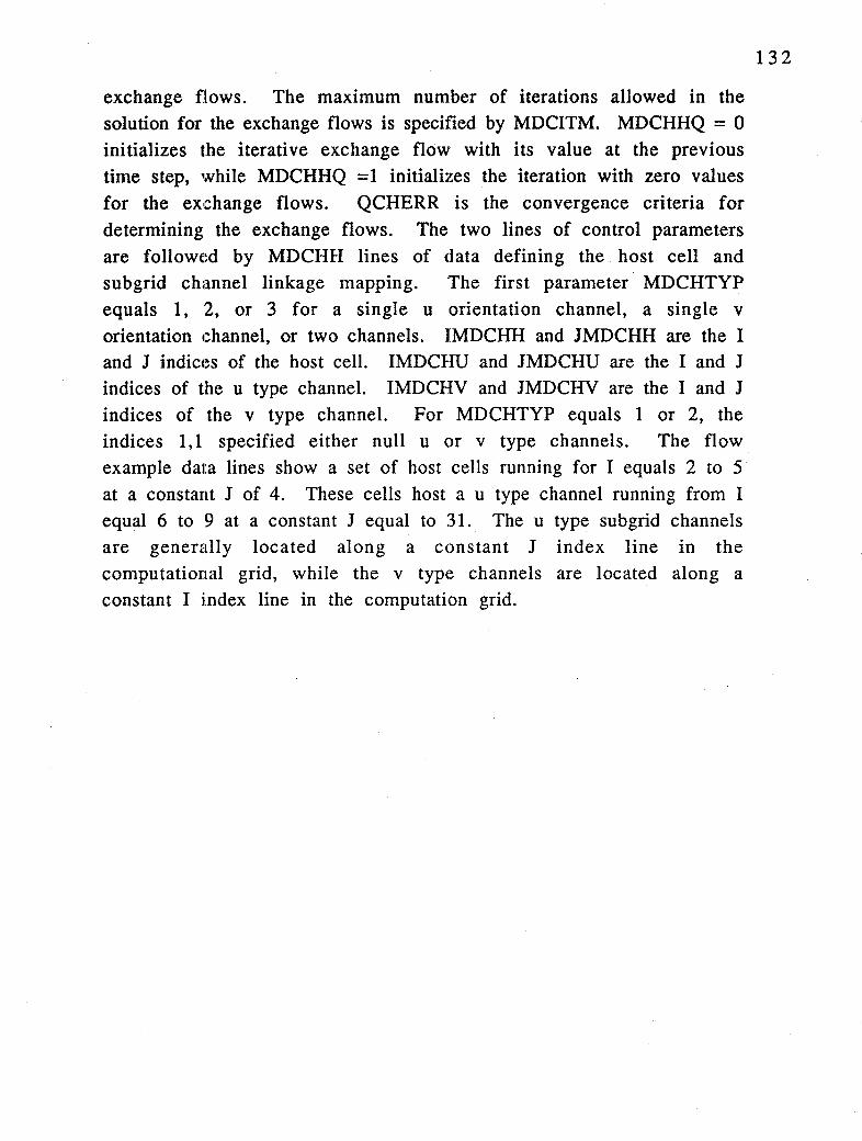
exchange flows. The maximum number of iterations allowed in the solution for the exchange flows is specified by MDCITM. MDCHHQ = 0 initializes the iterative exchange flow with its value at the previous time step, while MDCHHQ =1 initializes the iteration with zero values for the exchange flows. QCHERR is the convergence criteria for determining the exchange flows. The two lines of control parameters are followed by MDCHH lines of data defining the host cell and subgrid channel linkage mapping. The first parameter MDCHTYP equals 1, 2, or 3 for a single u orientation channel, a single v orientation channel, or two channels. IMDCHH and JMDCHH are the I and J indices of the host cell. IMDCHU and JMDCHU are the I and J indices of the u type channel. IMDCHV and JMDCHV are the I and J indices of the v type channel. For MDCHTYP equals 1 or 2, the indices 1, 1 specified either null u or v type channels. The flow example data lines show a set of host cells running for I equals 2 to 5 at a constant J of 4. These cells host a u type channel running from I equal 6 to 9 at a constant J equal to 31. The u type subgrid channels are generally located along a constant J index line in the computational grid, while the v type channels are located along a constant I index line in the computation grid.

132

Input file moddxdy.nnp

The file moddxdy .inp allows for quick modification of cell sizes, specified as dx and dy in the dxdy .inp file. Its primary use is for the quick adjustment of subgrid channel sections lengths and widths. The example below is self-explanatory.

C moddxdy.inp file, in free format across columns C NMDXDY =#of cells for DX(I,J)=RMDX*DX(I,J) & DY(I,J)=RMDX*DX(I,J) C I J RMDX RMDY C

4 6 7 8 9

31 31 31 31

1.0 1.0 1.0 1.0

2.5 2.5 2.5 2.5

133

Input file pser.inp

The input file pser.inp is used to specify surf ace elevation time series primarily for use at open boundaries. The file may contain multiple time series, each having a single control and conversion data line followed by a sequence of MP SER time data lines. An example is shown below.

C pser.inp file, in free format across line, repeats npser times C C C C C

MPSER(NS)

TPSER (M, NS)

4 265.00 270.00 273.00 275.00

TCPSER(NS)

PSER(M,NS)

86400. 4.90 4.90 4.90 2.06

TAPSER(NS) RMULADJ (NS) ADDADJ(NS)

! (rrpser (ns) pairs for ns=l,npser series)

0. 1.0 0.0

The parameter MPSER specifies the number of time data lines. TCPSER and TAPSER provide for adjustment and conversion of the time data units to seconds. RMULADJ and ADDADJ provide for conversion and adjustment of the elevation data to meters.

134

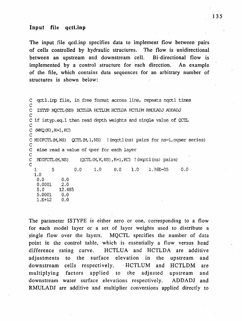
Input file qctl.inp

The input file qctl.inp specifies data to implement flow between pairs of cells controlled by hydraulic structures. The flow is unidirectional between an upstream and downstream cell. Bi-directional flow is implemented by a control structure for each direction. An example of the file, which contains data sequences for an arbitrary number of structures is shown below:

C qctl.inp file, in free format across line, repeats nqctl times C C ISTYP M):TL(NS) HCTLUA HCTLUM HCTIDA HCTIDM RMULADJ ADDADJ C C if istyp.E~.1 then read depth weights and single value of ():TL C C (WKQ (K), K==l, KC) C C HDIFCTL(M,NS) ():TL{M,l,NS) C

! (mqctl(ns) pairs for ns=l,nqser series)

C else read a value of qser for each layer C C HDIFCTL (M, NS) C

1 1.0

0.0 0.0001 5.0 5.0001 1.E+12

5

0.0 2.0

12.485 0.0 0.0

(OCTL (M, K, NS), K=l, KC) ! (mqctl (ns) pairs)

0.0 1.0 0.0 1.0 1.76E-05 0.0

The parameter ISTYPE is either zero or one, corresponding to a flow for each model layer or a set of layer weights used to distribute a single flow over the layers. MQCTL specifies the number of data point in the control table, which is essentially a flow versus head difference rating curve. HCTLUA and HCTLDA are additive adjustments to the surface elevation rn the upstream and downstream cells respectively. HCTLUM and HCTLDM are multiplying factors applied to the adjusted upstream and downstream water surface elevations respectively. ADDADJ and RMULADJ are additive and multiplier conversions applied directly to

135

the flow data and are useful for unit conversion. MQCTL data lines follow the one or two control data lines. The data pairs are elevation difference and flow. The data in · the above example implements the formula

Q == (1.7595£-5)(2.0+ 0.9(0.3048)(H,. +B,. -H"-B")) L

(x)

where QI L is discharge or flow per unit length and H and B are the water depth and bottom elevations in the upstream and downstream cells:

To illustrate the capabilities of the surface elevation or pressure flow control option it is convenient to summarize the sequence of steps involved in calculating the flow between the upstream and downstream cells. The FORTRAN statement sequence involves looping over all control structure pairs, NQCTL, and is shown in Table 6. The flow from the upstream cell to the downstream cell is determined by the difference, DELH, between the upstream pressure plus elevation head, HUP relative to -HCTLUA, adjusted by multiplying by HCTLUM, and the downstream pressure plus elevation head, HOW relative to -HCTLDA, adjusted by multiplying by HCTLDM. For flows controlled entirely by surface elevation differences, HCTLUA and HCTLDA would both be zero. For a spillway

or weir, -HCTLUA would be the spillway or weir crest elevation. For upstream only control, HCTLDM would be set to zero. Given the adjusted head difference, DELH, which must be greater than zero, the discharge or discharge per unit width, QCTLT, is determined from an interpolation table. A final multiplying adjustment, by RQCMUL, is applied to convert discharge per unit width to discharge if required. The hydraulic control structure option is also suitable for simulating water surf ace elevation controlled pump station operation.

136

500

C

DO NC'rL=l,NQCTL RQDW=l. IU=IQCTLU(NCTL) JU=JQCTLU(NCTL) LU=LIJ(IU, JU) HUP=HP(LU)+BELV(LU)+HCTLUA(NCTL) ID=IQCTLD(NCTL) JD=JQCTLD(NCTL) IF (ID.EQ.0.AND.JD.EQ.0) THEN

LD=LC HDW=O. RQDW=O.

ELSE LD=LIJ(ID, JD) HDW==HP (LD) +BELV (LD) +HCTLDA (NCTL)

END H'

I CELL INDEX UPSTREAM J CELL INDEX UPSTREAM L CELL INDEX UPSTREAM UPSTREAM SUF ELEV+ HCTLUA I CELL INDEX DOWNSTREAM J CELL INDEX DOWNSTREAM

FLOW OUT OF MODEL DOMAIN WITH UPSTREAM FLOW CONTROL

L CELL INDEX DOWNSTREAM UPSTREAM SUF ELEV+ HCTLDA

DELH=HCTLUM(NCTL)*HUP-HCTLDM(NCTL)*HDW ! ADJUSTED DIFFERENCE IF (DELH.LE.0.) THEN ! NO FLOW

DO K=l,KC QCTLT(K,NCTL)=O. END DO

ELSE Ml=O M2=l Ml=Ml+l M2=M2+1

ENTER INTERPOLATION TABLE TO DETERMINE FLOW IN EACH LAYER AS A FUNCTION OF DELH

IF(DELH.GE.HDIFCTL(Ml,NCTL) .AND.DELH.LE.HDIFCTL(M2,NCTL))THEN TDIFF=HDIFCTL(M2,NCTL)-HDIFCTL(Ml,NCTL) WI'Ml=(HDIFCTL(M2,NCTL)-DELH)/TDIFF WI'M.2=(DELH-HDIFCTL(Ml,NCTL))/TDIFF DO K=l,KC

QCTLT(K,NCTL)=WTMl*QCTL(Ml,K,NCTL)+WTM2*QCTL(M2,K,NCTL) END DO ! FLOW ASSIGNED TO LAYERS,K

ELSE GO TO 500

END IF END I1~

DO K==l, KC ! ADD CONTROL FLOW TO OTHERS QSUM(LU,K)=QSUM(LU,K)-RQCMUL(NCTL)*QCTLT(K,NCTL) QSUM(LD,K)=QSUM(LD,K)+RQCMUL(NCTL)*RQDW*QCTLT(K,NCTL) END DO

END DO

HP ( ) : BELV( ) : NQCTL: MQCTL: HCTLUA: HCTLUM: HCTLDA: HCTLDM: HDIFCTL: QCTL: RQCMUL:

Table 6.

CELL CENTER DEPTH CELL CENTER BOTTOM ELEVATION NUMBER OF CONTROLLED FLOW SETS NUMBER OF DEPTH FLOW PAIRS IN SET NS CONSTANT ADDED TO UPSTREAM ELEVATION UPSTREAM MULTIPLIER CONSTANT ADDED TO UPSTREAM ELEVATION DONWSTREAM MULTIPLIER DEPTH AND VOLUMETRIC FLOW PAIRS CONVERTS DISCHARGE/LENGTH TO DISCHARGE, =l FOR DISCHARGE, = DX OR DY FOR DISCHARGE PER LENGTH

FORTRAN Implementation of Control Structures

137

Input file qser.inp

An example: of the qser.inp file is shown below.

C qser.inp file, in free format across line, repeats nqser times C C ISTYP M;JSER(NS) TCQSER(NS) TAQSER(NS) RMULADJ(NS) ADDADJ(NS) C C if istyp.eq.1 then read depth weights and single value of QSER C C (WKQ (K), l:C=l, KC) C C TQSER(M,NS) QSER(M, 1,NS) ! (rnqser (ns) pairs for ns=l,nqser series) C C else read a value of qser for each layer C C TQSER(M,NS) (QSER(M,K,NS) ,K=l,KC) ! (mqser(ns) pairs) C

1 10 3600.0 0. 1. 0. 0 0.166 0.167 0.167 0.167 0.167 0.166

-2000.0000 0.00 713.39 0.00 713.41 0.001 726.89 0.001 726.91 0.00

7076.49 0.00 7076.51 0.001 7087.99 0.001 7088.01 0.00 10000.00 0.00 1 9 3600.0 0.0 1.0. 0. 0

0.166 0.167 0.167 0.167 0.167 0.166 708.0 260.3 732.0 243.3 756.0 230.2 780.0 215.9 804.0 202.3 828.0 192.9 852.0 181.1 876.0 182.9 900.0 173.5

138

Input file restart.inp

The file restart.inp is used to specify initial conditions for running the EFDC model in the restart mode. The file is obtained by renaming the restart.out file.

Input file restran.inp

The file restran.inp is used to specify advective and diffusive transport files when the EFDC model is executed in the transport only mode. The file is obtained by renaming the restran.out file.

Input file show.inp

The file show.inp, shown below, is used to control screen writing of information at the horizontal location specified by the horizontal cell indices !SHOW and JSHOW. The parameter NSTYPE determines the type of screen displace. For NSTYPE equal to 1, the screen display emulates

C show. inp file, in free format across line C C NSTYPE NSHcmR ISHOW: JSHCW: C C ZSSMIN ZSSMAX SSAI.MAX C

2 30 7 65 -3. 3. 8.

a strip chart recording of water surface elevation and surface and bottom salinity. In this mode, and lower and upper scale for the surface elevation, ZSSMIN and ZSSMAX and an upper scale for salinity, SSALMAX must be specified on the third data line. The file is reread every NSHOWR time steps. Between the rereads of the file, it may be edited (only on multiple window UNIX systems) to move

locations and the type of display. For NSTYPE equal 2, 3, or 4, column format data on time or timestep, surface and bottom layer

139

velocity, salinity or sediment concentration, and vertical diffusion coefficients are displayed. NSTYPE = 2 displays timestep and salinity. NSTYPE = 3 displays time in days and salinity. NS TYPE = 4 displays timestep a.nd sediment concentration. Activating this option is generally recommended for diagnostics of new applications and may result in noticeable decreases in model execution speeds on systems with slow IO capabilities.

Input file sfbser.inp

The file sfbser.inp specifies behavioral information for shellfish larvae when the shellfish larvae transport is activated. The header lines explain the meaning to the various time dependent behavior control information.

C sfbser.inp file, shellfish larvae behavior time series in free format C MSFSER=no of time data points. TCSFSER=converts time values to sec C TASFSER=additive adjustment to time values C TSRSF,TSSSF=times of sunrise and sun set as a fraction of 24 hours C ISSFLDN=l to activate daylight,darkness dependent behavior C ISSFLFE=l to activate flood,ebb dependent behavior C TSFSER=time of data RKDSFL=first order decay rate in 1/sec C WSFLST=settling velocity in m/s WSFLSM=vert swim velocity in m/s C DSFLMN=m:inimum depth below surface in daylight, meters C DSFLMX=maximum depth below surface in daylight, meters C SFNTBE=restricts advection in bottom layer during ebb C 0. equals full restriction, 1. equals no restriction C SFATBT=l. allows larvae to settle to bottom and attach C C MSFSER TCSFSER TASFSER TSRSF TSSSF ISSFLDN ISSFLFE C C TSFSER RKDSFL WSFLST WSFLSM DSFLMN DSFLMX SFNTBE SFATBT C

4 86400. 0. 0.25 0.84 1 1 -10000. 0. 0. 0. 0. o. 0. o. 0. o. 0. o. 0. 0. 0.01 0. o. 0. 0. 0. 0. 10000. 0. o. 0. o. 0. 0.

0. 0. 0. 0.

140

Input file vege.inp

The input file vege.inp specifies information on vegetation resistance. An example is shown below.

C vege.inp file, in free fonnat across line, vK:A2A C C MVEGTYP (:/t vege classes) MVEGOW (o:pen water class) UVEGSCL (vel scale) C C after reading MVEGTYP, MVEGOW and UVEGVSCL read MVEGTYP lines of vars C C M RDLPSQ BPVEG HPVEG AIPVEG BE'IVEG GAMVEG SCVEG C typ# 1/m**2 meters meters no dim no dim no dim nodim C

20 17 0.01 1 32.0 O.lE-0 2.5 0.7854 1.0 0.0 0.50 2 1B.O O.lE-0 2.5 0.7854 1.0 0.0 0.50 3 B.O O.lE-0 2.5 0.7854 1.0 0.0 0.50 4 26.0 O.lE-0 2.5 0.7854 1.0 0.0 0.50 5 12.0 O.lE-0 2.5 0.7854 1.0 0.0 0.50 6 32.0 O.lE-0 2.5 0.7854 1.0 0.0 0.50 7 32.0 O.lE-0 2.5 0~7854 1.0 0.0 0.50 8 18.0 O.lE-0 2.5 0.7854 1.0 0.0 0.50 9 12.0 O.lE-0 2.5 0.7854 1.0 0.0 0.50

10 32.0 O.lE-0 2.5 0.7854 1.0 0.0 0.50 11 18.0 O.lE-0 2.5 0.7854 1.0 0.0 0.50 12 B.O O.lE-0 2.5 0.7854 1.0 0.0 0.50 13 26.0 O.lE-0 2.5 0.7854 1.0 0.0 0.50 14 18.0 O.lE-0 2.5 0.7854 1.0 0.0 0.50 15 26.0 O.lE-0 2.5 0.7854 1.0 0.0 0.50 16 32.0 O.lE-0 2.5 0.7854 1.0 0.0 0.50 17 0 .. 25 O.lE-0 2.5 0.7854 1.0 0.0 0.50 18 32.0 O.lE-0 2.5 0.7854 1.0 0.0 0.50 19 32.0 O.lE-0 2.5 0.7854 1.0 0.0 0.50 20 B.O O.lE-0 2.5 0.7854 1.0 0.0 0.50

The parameter MVEGTYP specifies the number of vegetation types. The vegetation is represented as cylindrical elements of height HPVEG and width or diameter BPVEG having a spatial density of RDLPSQ resistance elements per square meter. The parameter ALPVEG, BETVEG, GAMVEG, and SCVEG are dimensionless shape factors (see Hamrick and Moustafa, 1995a) with the values shown being typical of cattail and sawgrass.

141

Input file wave.inp

The file wave.inp is used to specify forcings for induced cmTents and wave-current boundary layers. on the header lines define and explain the various

modeling wave The definitions data types. A

preprocessor is available from the author to generate the two layer data sets required in this file using the output of various wave prediction and transformation models.

142

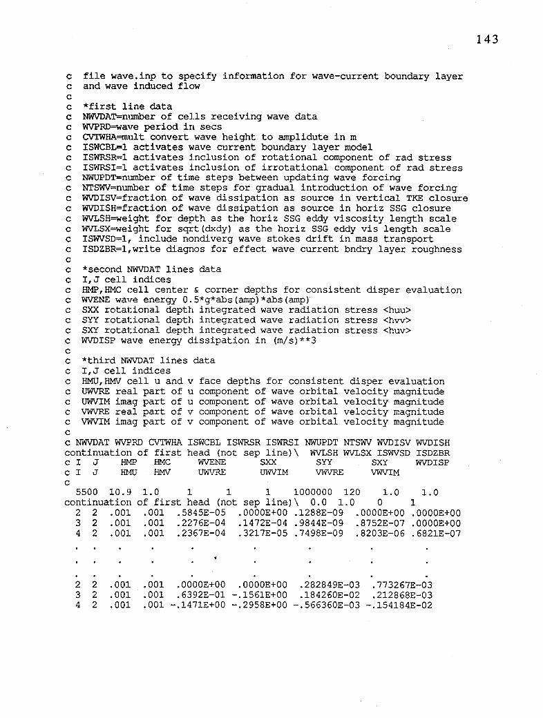
c file wavE~.inp to specify information for wave-current boundary layer c and wave induced flow C

c *first line data c NWVDAT=number of cells receiving wave data c WVPRD--wave period in secs c CVTWHA=mult convert wave height to arnplidute in m c ISWCBL=l activates wave current boundary layer model c ISWRSR=l activates inclusion of rotational component of rad stress c ISWRSI=l activates inclusion of irrotational component of rad stress c NWUPDT=nurnber of time steps between updating wave forcing c NTSWV=number of time steps for gradual introduction of wave forcing c WVDISV=fraction of wave dissipation as source in vertical TKE closure c WVDISH=fraction of wave dissipation as source in horiz SSG closure c WVLSH=weight for depth as the horiz SSG eddy viscosity length scale c WVLSX=weight for sqrt(dxdy) as the horiz SSG eddy vis length scale c ISWVSD=l, include nondiverg wave stokes drift in mass transport c ISDZBR=l,write diagnos for effect wave current bndry layer roughness C

c *second NWVDAT lines data c I,J cell indices c HMP,HMC cell center & corner depths for consistent disper evaluation c WVENE wave energy 0.5*g*abs(arnp)*abs(arnp) c SXX rotational depth integrated wave radiation stress <huu> c SYY rotational depth integrated wave radiation stress <hvv> c SXY rotational depth integrated wave radiation stress <huv> c WVDISP wave energy dissipation in (m/s)**3 C c *third NWVDAT lines data c I,J cell indices c HMU,HMV cell u and v face depths for consistent disper evaluation c UWVRE real part of u component of wave orbital velocity magnitude c UWVIM imag part of u component of wave orbital velocity magnitude c VWVRE real part of v component of wave orbital velocity magnitude c VWVIM imag part of v component of wave orbital velocity magnitude C

c NWVDAT WVl?RD CVTWHA ISWCBL ISWRSR ISWRSI continuation of first head (not sep line)\

NWUPDT NTSWV WVDISV WVDISH WVLSH WVLSX ISWVSD ISDZBR

c I J HMP HMC WVENE SXX SYY SXY WVDISP c I J HMU HMV UWVRE UWVIM VWVRE VWVIM C

5500 10.9 continuation

2 2 3 2 4 2

2 2 3 2 4 2

.001

.001

.001

.001

.OOJ.

.001

1.0 1 1 1 1000000 120 1. 0 1.0 of first head (not sep line)\ 0.0 1. 0 0 1

.001 .5845E-05 .OOOOE+OO .1288E-09 .OOOOE+OO .OOOOE+OO

.001 .2276E-04 .1472E-04 .9844E-09 .8752E-07 .OOOOE+OO

.001 .2367E-04 .3217E-05 .7498E-09 .8203E-06 .6821E-07

.001 .OOOOE+OO .OOOOE+OO .282849E-03 .773267E-03

.001 .6392E-01 -.1561E+OO .184260E-02 .212868E-03

.001 -.1471E+OO -.2958E+OO -.566360E-03 -.154184E-02

143

6. Compiling and Executing the Code

To compile the EFDC model, the FORTRAN 77 source code efdc.f and the include files efdc.com, which contains global common blocks, and efdc.par, which contains a global parameter statement are necessary and should reside ,in the same directory. Extensive efforts have been made to ensure cross-platform compatibility of the EFDC model, however, a number of minor modifications are required for various platforms. The source code efdc.f contains calls to the VMS time utility secnds. For compilers which support the secnds function through systems libraries, (DEC and Hewlett-Packard UNIX systems and Absoft and LSI Macintosh FORTRAN compilers), no modifications to the standard source efdc.f are required if appropriate compiler options are specified. (To determine if your compiler supports the secnds functions, look for secnds or VMS compatibility in the compiler reference manuals.) For compilers which do not support the secnds function, (Cray cf77, Sun UNIX) the real function subroutine secnds.f should be appended to the end of the standard source code. A somewhat less desirable fix is to comment out calls to the secnds function. Many of the IO operations in the efdc.f source code use the open file statement form:

OPEN(l ,FILE='fname', STATUS='UNKNOWN',ACCESS='APPEND')

To the writer's knowledge, the only systems which do not support the ACCESS='APPEND' modifier are Cray and IBM Risc6000 UNIX Systems. For Cray compilation, the ACCESS='APPEND' should be globally replaced by POSITION='APPEND'. A Cray-compatible version of the source, cefdc.f is continually maintained and available by ftp as described in the fore word of this report.

Except for the optional function subroutine secnds.f, the source code consisting of approximately 112 subroutines at last count is maintained as a single text file, efdc.f or cef dc.f. A number of compilers, including the Cray and Silicon Graphics UNIX compilers

144

and the Lahey Intel based PC compiler, are able to produce optimized executable code by operating the entire source using, for example, the Cray and SGI commands:

cf77 -Zv cefdc.f f77 -03 ef dc.f

which produce the executable a.out. (Note the option -Zv for the Cray compilation produces optimum vectorization, using -Zp would produce both optimum vectorization and autotasking). Other compilers, such as the HP and SUN UNIX compilers and the Absoft and LSI Macintosh compilers, are capable of producing only nonoptimized executables working with the entire source code. An example command line for the HP is:

f77 -K +El -C -o hpefdcnopt efdc.f

which produces the nonoptimized executable hpefdcnopt. The options -K +El invoke support of the secnds function, while -C implements array range checking. To produce optimized code on these systems, recourse to makefiles or batch command files which compile each subroutine separately is necessary. Batch command

files for HP and SUN UNIX compilers and Makefiles for Absoft and LSI Macintosh compilers are available via ftp.

To achieve minimum memory requirements for running a specific application, it is recommended that the parameter file be customized for that application. The parameter file is of the form:

145

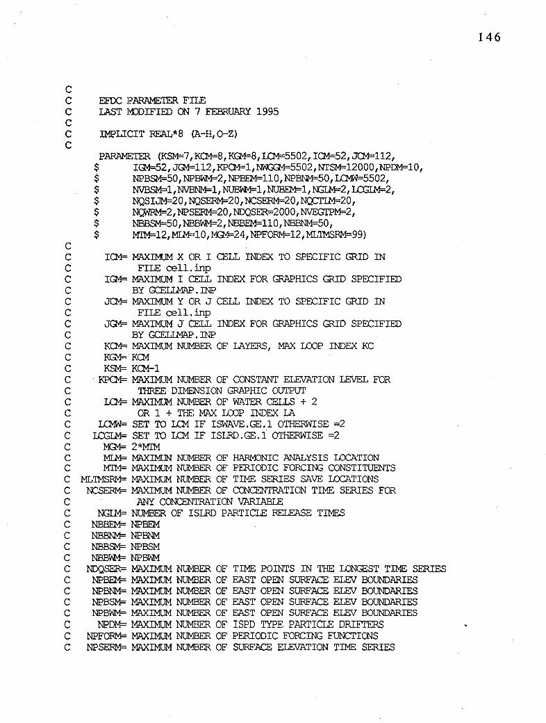
146

C C EEOC PARAMETER FILE C LAST 1'1)DIFIED ON 7 FEBRUARY 1995 C C IMPLICIT REAL*8 (A-H, 0-Z) C

PARAMl~TER (KSM=7,K01=8,KG1=8,LCM==5502,IQ1=52,JCM=ll2, $ IG1=52,JQ.1:::112,KP01=1,NWGCM=5502,NI'SM=l2000,NPDM=l0, $ NPBSM=50,NPBWM=2,NPBEM=110,NPBNM=50,LCMW=5502, $ NVBSM=l, NVBNM=l, N'Ua'M=l, NUBEM= 1, N:iI.M=2, LCGI.M=2, $ NQSIJM=20,NQSERM=20,NCSERM=20,NQ::TIM=20, $ NQWRM=2,NPSERM=20,NDQSER=2000,NVEGI'PM=2, $ NBBS1=50, NBBWM=2, NBBEM=llO, NBBNM=50, $ MIM=l2,MI.M=l0,~24,NPFORM=12,ML'IMSRM=99)

C C IQ1= MAXIMUM XOR I CELL INDEX TO SPECIFIC GRID IN C FILE cell.inp C IGM= MAXIMUM I CELL INDEX FOR GRAPHICS GRID SPECIFIED C BY GCELI.MAP. INP C JCM= MAXIMUM Y OR J CELL INDEX 'I'O SPECIFIC GRID IN C FILE cell.inp C J(M= MAXIMUM J CELL INDEX FOR GRAPHICS GRID SPECIFIED C BY GCELll-1AP • INP C K01= MAXIMUM NUMBER OF IAYERS, ~ LCX)P INDEX KC C KGM= KCM C KSM= KCM-1 C - KPQ1= MAXIMUM NUMBER OF CCNSTANT ELEVATION LEVEL FOR C THREE DIMENSION GRAPHIC OUTPUT C 101= MAXIMUM NUMBER OF WATER CELLS + 2 C OR 1 + THE MAX LOOP INDEX IA C LCMW= SET TO LCM IF ISWAVE.GE.1 OTHERWISE =2 C LCGI.M= SET TO LCM IF ISLRD.GE.1 OTHERWISE =2 C t-01= 2*MIM C MI.M= MAXIMUN NUMBER OF HARM'JNIC .ANALYSIS LOCATION C MI'M= MAXIMUM NUMBER OF PERIODIC FORCIN3 CONSTITUENTS C ML'IMSRM= MAXIMUM NUMBER OF TIME SERIES SAVE LOCATICNS C NCSERM= MAXIMUM NUMBER OF CCNCENTRATION TIME SERIES FOR C ANY CONCENTRATICN VARIABLE C NGLM= NUMBER OF ISLRD PARTICLE RELEASE TIMES C NBBEM= NPBEM C NBBNM= NPPNM C NBBSM= NPBSM C NBBvM= NPBWM C NDQSER= MAXIMUM NUMBER OF TIME POINI'S IN THE LONGEST TIME SERIES C NPBEM= MAXIMUM NUMBER OF EAST OPEN SURFACE ELEV BOUNDARIES C NPBNM= MAXIMUM NUMBER OF EAST OPEN SURFACE ELEV BOUNDARIES C NPBSM= MAXIMUM NUMBER OF EAST OPEN SURFACE ELEV BOUNDARIES C NPBWM= MAXIMUM NUMBER OF EAST OPEN SURFACE EIEV BOUNDARIES C NPDM= MAXIMUM NUMBER OF ISPD TYPE PARTICLE DRIFTERS C NPFORM= MAXIMUM NUMBER OF PERIODIC FORCING FUNCTICNS C NPSERM= MAXIMUM NUMBER OF SURFACE ELEVATION TIME SERIES

C NCCTIM= MAXIMJM NUMBER OF FI..(M CONTROL STRUCTURES C NQSERM= MAXIMUM NUMBER OF FI..(M TIME SERIES C NQSIJM= MAXIMUM NUMBER OF NQSIJ VOLUMETRIC SOURCE-SINKS C N;:;lWRM= MAXIMJM NUMBER OF FI..(M WITH-RETURN PAIRS C NTSM= MAXIMUM NU1BER OF TIME STEP PER REFERENCE TIME PERIOO C NUBEM= 1 C NUBvM= 1 C NVBN.J,= 1 C NVBSM= 1 C Nvml'PM= MAXIMJM NUMBER OF VEGETATION TYPE CLASSES C ~ NUMBER OF WATER CELLS IN CARTESIAN GRAPHIC OVERLAY C GRID, EQUAL TO LO:vi-2 FOR CARTESIAN GRIDS C

For a given model application, the parameters, which dimension arrays in efdc.com, should be set to the lowest value that accommodates the grid and data for the application. When starting to run a new application, it is recommended to use a nonoptimized executable compiled with the range checking option (usually -C on UNIX compilers) to determine if anayed variables are within the range specified by the parameter dimensioned arrays.

147

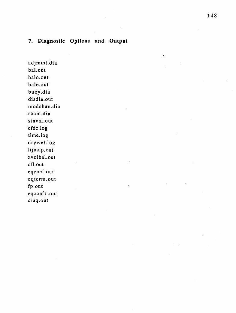
7. Diagnostic Options and Output

adjmmt.dia bal.out halo.out bale.out buoy.dia disdia.out modchan.dila rbcm.dia sinval.out efdc.log time.log drywet.log lijmap.out zvolbal.out cfl.out eqcoef.out eqterm.out fp.out eqcoefl .out diaq.out

148

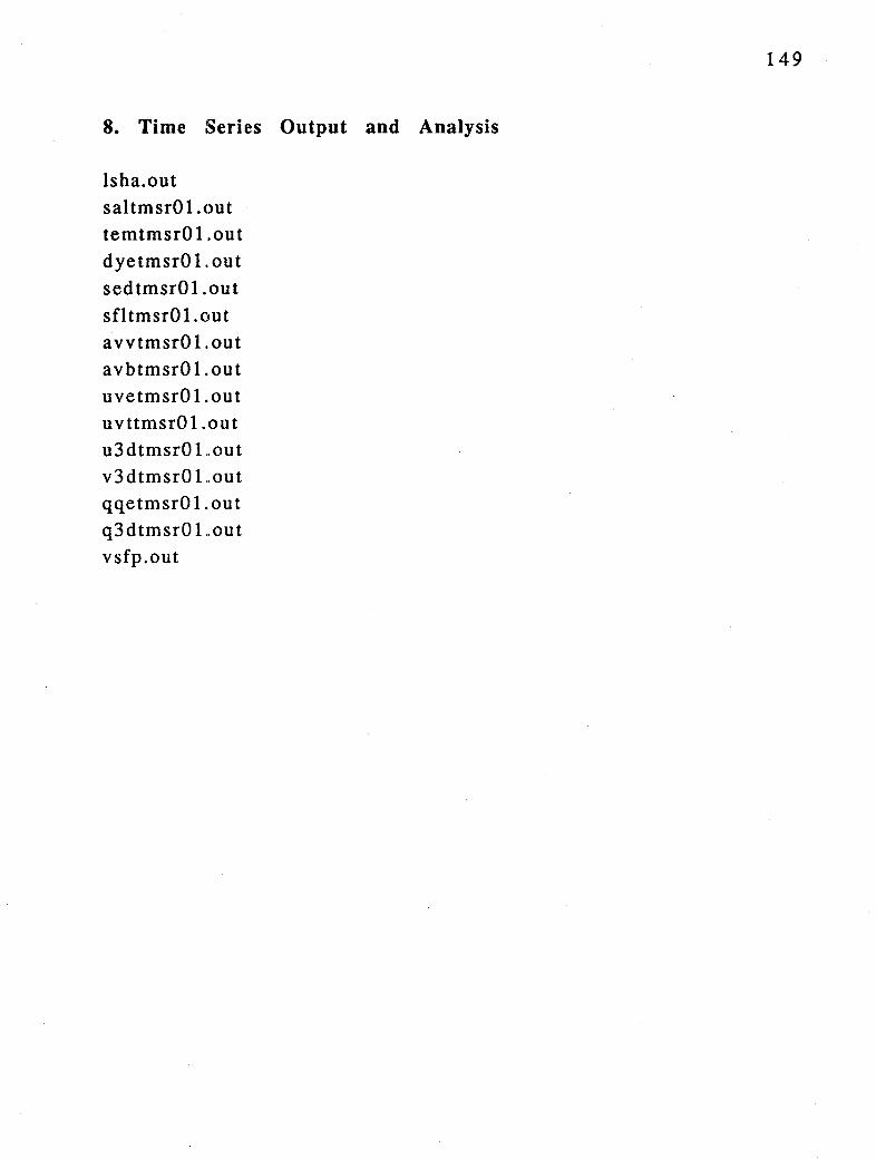
8. Time Series Output and Analysis

lsha.out saltmsrOl .out temtmsrO Lout dyetmsrO Lout sedtmsrOl .out sfl tmsrO 1. out avvtmsrO 1. out avbtmsrOl .out uvetmsrOl.out uvttmsrOl .out u3dtmsr01..out v3dtmsr01..out qqetmsrOl.out q3dtmsr01..out vsfp.out

149

150

INSTANTANEOUS VERTICAL SCALAR FIEID PROFIIES

TIME= 3221.6001 N = 1665 I,J = 151 42 DEPTH BEWW SURFACE IDDEL SALINITY

1.00 16.70 3.00 17.27 5.00 17.79 7.00 18.09 9.00 18.21

11.00 18.24 13.00 18.25

TIME= 3222.0000 N = 1679 I,J = 140 46 DEPTH BEI.DW SURFACE M)DEL SALINITY

1.00 17.36 3.00 17.37 5.00 17.37 7.00 17.37 9.00 17.39

11.00 17.42 13.00 17.43 15.00 17.44 17.00 17.44 19.00 17.45

TIME= 3222.3999 N = 1693 I,J = 124 59 DEPTH BELOW SURFACE M)DEL SALINITY

1.00 13.51 3.00 13.51 5.00 14.53 7.00 14.93

9.00 14.93

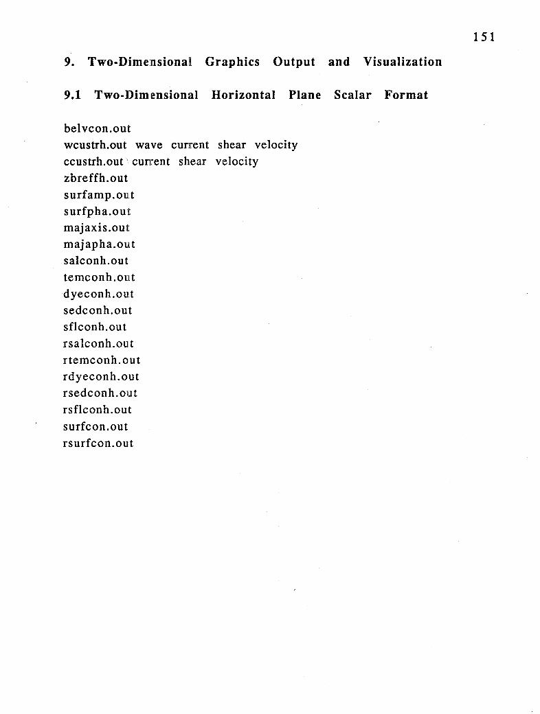
9. Two-Dimensional Graphics Output and Visualization

9.1 Two-Dim,ensional Horizontal Plane Scalar Format

belvcon.out wcustrh.out wave current shear velocity ccustrh.out ·. cunrent shear velocity zbreffh.out surfamp.ou1t surfpha.out majaxis.out majapha.out salconh.out temconh.out dyeconh.ou.t sedconh.out sflconh.out rsalconh.out rtemconh.out rdyeconh.out rsedconh.out rsflconh.out surf con.out rsurfcon.out

151

9.2 Two-Dim1ensional Horizontal Plane Vector Format

tstvech.out stvech.out tauvech.out tidelkc.out tidelkb.out velvech.out rvelvech.out pvelvech.out mvelvech.out lmvvech.out almvvech.out

152

9.3 Two-Dimensional Vertical Plane Scalar Format

salcnv Lout temcnv I .out dyecnvLout sedcnv I .out sflcnv Lout rsalcnv I .out rviscnv I .out rvefcnv I .out rsflcnvl .out velcnvLout rvelcnvLout pvelcnvLout mvelcnvl .out lmvcnv I .out almvcnv I .out rvelcvtI .out pvelcvtl .out mvelcvtI .out lmvcvtI .out almvcvtI .out

9.4 Two-Dim1ensional Vertical Plane Vector Format

velvcvLout rvelvcvl .out pveivcvLout mvelvcv I .out lmvvcv I .out almvvcv I .out

153

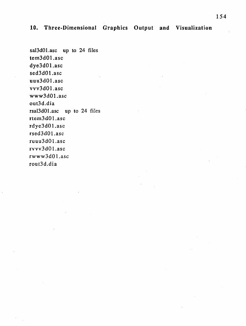
10. Three-Dimensional Graphics Output and Visualization

sal3d01.asc up to 24 files tem3d01.asc dye3d01.asc sed3d0 Lase uuu3d01.asc vvv3d01.asc www3d01.asc out3d.dia rsal3d01.asc up to 24 files rtem3d01.asc rdye3d01.asc rsed3d01.asc ruuu3d01.asc rvvv3d01.asc rwww3d01.asc rout3d.dia

154

11. Miscellaneous Output

efdc.out avsel.out gwelv.out cell9.out drifter.out restran.out restart.out waspp.out waspc.out waspb.out waspd.out waspdhd.out waspdh.out waspdhu.out advmod.wsp <listen.out uvtsc.out uverv .out

155

12. References

Ambrose, R. B., T. A. Wool, and J. L. Martin, 1993: The water quality analysis simulation program, WASPS. U. S. Environmental Protection Agency, Environmental Research Laboratory, Athens, GA, 210 pp.

Bennett, A. F., 1976: Open boundary conditions for dispersive waves. J. Atmos. Sci., 32, 176-182.

Bennett, A. F., and P. C. McIntosh, 1982: Open ocean modeling as an inverse problem: tidal theory. J. Phys. Ocean., 12, 1004-1018.

Bennett, J. R., and A. H. Clites, 1987: Accuracy of trajectory calculation in a finite-difference circulation model. J. Comp. Phys., 68, 272-282.

Blumberg, A. F., and L. H. Kantha, 1985: Open boundary condition for circulation models. J. Hydr. Engr., 111, 237-255.

Blumberg, A. F., and G. L. Mellor, 1987: A description of a threedimensional coastal ocean circulation model. In: Three-Dimensional Coastal Ocean l'Jodels, Coastal and Estuarine Science, Vol. 4. (Heaps, N. S., ed.) American Geophysical Union, pp. 1-19.

Chikhliwala, E. D., and Y. C. Yortsos, 1985: Application of orthogonal mapping to some two-dimensional domains. J. Comp. Phys., 57, 391-402.

Galperin, B., L. H. Kantha, S. Hassid, and A. Rosati, 1988: A quasiequilibrium turbulent energy model for geophysical flows. J. Atmos. Sci., 45, 55-62.

Cereo, C. F., and T. Cole, 1993: Three-dimensional eutrophication model of Chesapeake Bay. J. Environ. Engnr., 119, 1006-1025.

Glenn, S. M., and W. D. Grant, 1987: A suspended sediment stratification correction for combined wave and current flows. J. Geophys. Res., 92, 8244-8264.

Grant, W. D., and 0. S. Madsen, 1982: Movable bed roughness in unsteady oscillatory flow. J. Geophys. Res., 87, 469-482.

156

Hamrick, J. M., 1991: Analysis of m1xmg and dilution of process water discharged into the Pamunkey River, a Report to the Chesapeake Corp. The College of William and Mary, Virginia Institute of Marine Science, 50 pp.

Hamrick, J. M[., 1992a: A Three-Dimensional Environmental Fluid Dynamics Computer Code: Theoretical and Computational Aspects. The College of William and Mary, Virginia Institute of Marine Science. Speciall Report 317, 63 pp.

Hamrick, J. M., 1992b: Estuarine environmental impact assessment using a three-dimensional circulation and transport model. Estuarine and Coastal Modeling, Proceedings of the 2nd International Conference, :M. L. Spaulding et al, Eds., American Society of Civil Engineers, New Yrok, 292-303.

Hamrick, J. M.,. 1992c: Preliminary analysis of mixing and dilution of discharges into the York River, a Report to the Amoco Oil Co. The College of William and Mary, Virginia Institute of Marine Science, 40 pp.

Hamrick, J. M., 1994a: Linking hydrodynamic and biogeochemical transport models for estuarine and coastal waters. Estuarine and Coastal Modeling, Proceedings of the 3rd International Conference, M. L. Spaulding et al, Eds., American Society of Civil Engineers, New York, 591-608.

Hamrick, J. M., 1994b: Evaluation of island creation alternatives in the Hampton Flats of the James River. a report to the U. S. Army Corps of Engineers, Norfolk District.

Hamrick, J. M., 1995a: Calibration and verification of the VIMS EFDC model of the James River, Virginia. The College of William and Mary, Virginia Institute of Marine Science, Special Report, in preparation.

Hamrick, J. M., 1995b: Evaluation of the environmental impacts of channel deepening and dredge spoil disposal site expansion in the lower James River, Virginia. The College of William and Mary, Virginia Institute of Marine Science, Special Report, in preparation.

157

Hamrick, J. M., and Z. Yang, 1995: Lagrangian mean descriptions of long-term eshiarine mass transport. Proceeding of the 1994 International Conference on the Physics of Estuaries and Bays. D. Aubrey, Ed., American Geophysical Union, in press.

Hamrick, J. M., and M. Z. Moustafa, 1995a: Development of the Everglades wetlands hydrodynamic model: 1. Model formulation and physical processes representation. submitted to Water Resources Research.

Hamrick, J. M., and M. Z. Moustafa, 1995b: Development of the Everglades wetlands hydrodynamic model: 2. Computational implementation of the model. submitted to Water Resources Research.

Johnson, B. H., K. W. Kim, R. E. Heath, B. B. Hsieh, and H. L. Butler, 1993: Validatiion of three-dimensional hydrodynamic model of Chesapeake Bay. J. Hyd. Engrg., 119, 2-20.

Knupp, P. M., 1992: A robust elliptic grid generator. J. Comp. Phys., 100, 409-418.

Mellor, G. L., and T. Yamada, 1982: Development of a turbulence closure model for geophysical fluid problems. Rev. Geophys. Space Phys., 20, 851-875 .

. Mobley, C. D., and R. J. Stewart, 1980: On the numerical generation of boundary-fitted orthogonal Curvilinear coordinate systems. J. Comp. Phys., 34, 124-135.

Moustafa, M. Z., and J. M. Hamrick, 1994: Modeling circulation and salinity transport in the Indian River Lagoon. Estuarine and Coastal Modeling, Proceedings of the 3rd International Conference, M. L. Spaulding et al, Eds., American Society of Civil Engineers, New York, 381-395.

Moustafa, M. Z., and J. M. Hamrick, 1995: Everglades wetlands hydrodynamic model: 3. South Florida water conservation area 2a. Resources Research.

Development of the Model application to submitted to Water

158

Moustafa, M. Z., J. M. Hamrick, and M. R. Morton, 1995: Calibration and verification of a limited area circulation and transport model of the Indian River Lagoon. submitted to Journal of Hydraulic Engineering.

Rennie, S., and J. M. Hamrick, 1992: Techniques for visualization of estuarine and c:oastal flow fields. Estuarine and Coastal Modeling, Proceedings of the 2nd International Conference, M. L. Spaulding et al, Eds., Americ:an Society of Civil Engineers, New York, 48-55.

Rosati, A. K., and K. Miyakoda, 1988: A general circulation model for upper ocean simulation. J. Phys. Ocean., 18, 1601-1626.

Ryskin, G. and L. G. Leal, 1983: Orthogonal mapping. J. Comp. Phys., 50, 71-100.

Smogorinsky, J., 1963: General circulation experiments with the primative equations, Part I: the basic experiment. Mon. Wea. Rev., 91, 99-152.

Smolarkiewicz, P. K., 1984: A fully multidimensional pos1t1ve definite advection transport algorithm with small implicit diffusion. J. Comp. Phys., 54, 325--362.

Smolarkiewicz, P. K., and T. L. Clark, 1986: positive definit1~ advection transport algorithm: and applications. J. Comp. Phys., 61, 396-438.

The multidimensional further development

Smolarkiewicz, P. K., and W. W. Grabowski, 1990: The multidimensional positive definite advection transport algorithm: nonoscillatory option. J. Comp. Phys., 86, 355-375.

Smolarkiewicz, P. K., and L. G. Margolin, 1993: On forward-in-time differencing for fluids: extension to a curvilinear framework. Mon. Weather Rev., 121, 1847-1859.

Zalesak, S. T. , 1979: Fully multidimensional flux-corrected transport algorithms for fluids. J. Comp. Phys., 31, 335-362.

159

Appendix A. Functions.

Subroutine

ADJMMT.f

AINIT.f

ASOLVE.f

ATIMES.f

CALAVB.f

CALBALI.f

CALBAL2.f

CALBAL3.f

CALBAL4.f

CALBAL5.f

CALBUOYI

CALCONCI

CALCSERI

160

EFDC Source Code Subroutines and Their

Function

Adjust mean transport field for transport only simulations

Initializes Variables

Utility solver for bi-conjugate gradient solver

Utility sparse matrix multiplier for bi-conjugate gradient solver

Calculates vertical turbulent viscosity and diffusivity

Calculates mass, momentum and energy balances





Calculates buoyancy or density anomaly using UNESCO equation of state

Calculates scalar field (concentration) transport

Concentration time series processor

CALDIFF.f

CALD1SP2.f

CALlD1SP3.f

CALEBl.f

CAUOO'.f

CAUQCi

CALHDMF.f

CALHEAT.f

CALHTA.f

CALlv.lMT.f

CALPSER.f

CALPUV.f

CALPUV2.f

CALPUV5.f

CALPUV7.f

Calculates horizontal diffusion of scalar fields

Calculates time average horizontal shear dispersion tensor

Calculates time average horizontal shear dispersion tensor

Calculates buoyancy integral in external mode equations

Calculates explicit terms in momentum equations

Calculates mass (scalar concentration field) sources and sinks

Calculates horizontal diffusion m momentum equations

Calculates surface and internal heat sources and sinks

Performs harmonic analysis for single frequency periodically forced flow

Calculates time mean mass transport field including Stokes' drift

Processes surface elevation time series

External mode solver for rigid lid or small surface displacement flows

External mode solver for larger surface displacements, but no drying or wetting

External mode solver for flows with drying and wetting and subgrid scale channels

External mode solver for kinematic wave approximation

161

CALQQl.f

CALQQ2.f

CALQVS.f

CALSED.f

CALSED2.f

CALSED3.f

CALSFf.f

CALTBXY.f

CALTRAN.f

CALTRANI.f

CALIRANQ.f

CALTRWQ.f

CALTSXY.f

CALUVW.f

Calculates transport of turbulent kinetic energy and length scale

Calculates transport of turbulent kinetic energy and length scale (research version)

Processes volumetric source and sink time series

Calculates cohesive sediment settling, deposition and resuspension

Calculates cohesive sediment settling, deposition and resuspension

Calculates noncohesive sediment settling, deposition and resuspension

Calculates diffusion, sources and sinks and vertical migration of shellfish larvae.

Calculates bottom drag coefficients for bottom stress calculation and calculates certain vegetation resistance parameters.

Calculates explicitly advective transport of scalar field concentration) variables

Calculates implicit advective transport of scalar field concentration) variables

Calculates advective transport of turbulent kinetic energy and length scale

Calculates explicit advection of water quality variables

Processes wind and atmospheric condition time series and calculates surface wind stress.

Solves the internal mode momentum equations and continuity equation

162

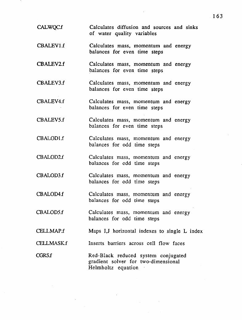
CAL'WQC.f

CBALEVl.f

CBALEV2.f

CBALEV3.f

CBALEV4.f

CBALEV5.f

CBALOD1.f

CBALOD2.f

CBALOD3.f

CBALOD4.f

CBALOD5.f

CELLMAP.f

CELLMASK.f

CGRSi

Calculates diffusion and sources and sinks of water quality variables

Calculates mass, momentum and energy balances for even time steps





Calculates mass, momentum and energy balances for odd time steps





Maps I,J horizontal indexes to single L index

Inserts barriers across cell flow faces

Red-Black reduced system conjugated gradient solver for two-dimensional Helmholtz equation

163

CONGRADf

DEPPLT.f

DEPSMfH.f

DRIFTER.f

EAX'.f

FILTRAN.f

GLMRES.f

HDMT.f

INPUT.f

LAGRES.f

LINBCG.f

LSQHARM.f

LTMT.f

LUBKSBi

LUDC:MP.f

Diagonally preconditioned conjugated gradient solver for two-dimensional Helmholtz equation

Generates file for bathymetry contouring in ASCII column format

Smoothes bottom elevation and initial depth fields

Releases and tracks Lagrangian drifters at specified times and locations

Main program

Performs vertical filtering of mean mass transport field

Calculates generalized Lagrangian mean velocities

Controls hydrodynamic and mass transport solution

Processes input files

Calculates Lagrangian mean velocities by forward trajectories

Bi-conjugate gradient linear equation solver

Performs least squares harmonic analysis

Controls mass transport only solution

Back substitution utility for LU decomposition equation solver

LU decomposition equation solver

Writes ASCII column files for visualization of Lagrangian mean velocity field in horizontal stretched layer

164

LVELPLTV.f

OUT3D.f

OUTPUTl.f

OUTPUT2.f

PPLOT.f

REDKCi

REUUC.f

RELJUCV.f

RESTINl.f

RESTIN10.f

RESTIN2.f

RES1M0D.f

RES1DUTJ

RESTRAN.f

Writes ASCII column files for visualization of Lagrangian mean velocity field in vertical transects

Writes files for two-dimensional slice and three-dimensional volume visualization of vector and scalar fields in 8 bit ASCII integer format or 8 bit HDF integer format

Writes printer output files in crude printer character contouring form

Writes printer output files in crude printer character contouring form

Processes printer character contour plots

Reduces layers by 1/2 in mass transport only simulations (not active)

Solve two-dimensional Helmholtz equation by Red-Black SOR (successive over relaxation)

A more vectorizabe version of RELAX.f

Reads restart.inp file for restarting a run

Reads older versions of restart.inp

Reads a K layer restart.inp file to initialize a 2 *K layer simulation

Reads restart.inp field and deactivates specified horizontal cell

Writes restart file restart.out

. Reads transport file restran.inp for transport only simulations

165

ROUT3D.f

RSALPLTH.f

RSALPLTV.f

RSURFPLT.f

RVELPLTH.f

RVELPLTV.f

SALPLTH.f

SALPLTV.f

SALTSMTH.f

SECNDSJ

Writes files for two-dimensional slice and three-dimensional volume visualization of time mean vector and scalar fields in 8 bit ASCII integer format or 8 bit HOF integer format

Writes ASCII column files for time means scalar field visualization in horizontal stretched layers

Writes ASCII column files for time mean scalar field visualization in vertical transects

Writes ASCII column file for visualization of time mean surface displacement field

Writes ASCII column files for visualization of time mean velocity field in horizontal stretched layers

Writes ASCII column files for visualization of time mean velocity field in vertical transects

Writes ASCII column files for instantaneous scalar field visualization in horizontal stretched layers

Writes ASCII column files for instantaneous scalar field visualization in vertical transects

Smoothes or interpolates an initial salinity field for cold start runs

Emulates VMS library function secnds on compilers not supporting this function. This is the only optional subroutine in the code and is normally appended to the end of the ef dc.f file for compilation on certain UNIX and Intel based PC compilers.

166

SEI'BCS.f

SNRM:J

SURFPLT.f

SVBKSB.f

SVDC:MP.f

TMSR.f

VALKH.f

VELPLTH.f

VELPLTV.f

VMSLIB.f

VSFP.f

WASP4.f

Set horizontal boundary conditions

Writes screen dlisplay of instantaneous conditions at a specified horizontal location

Computes error norm for bi-conjugate gradient equation solver

Writes ASCII column files for instantaneous surface displacement visualization

Back substitution utility of SYD equation solver

SYD (Singular value decomposition) linear equation solver

Writes time series files

Real function subroutine to solve high frequency surface gravity wave dispersion relationship for kh.

Writes ASCII column files for visualization of instantaneous velocity field in horizontal stretched layer

Writes ASCII column files for visualization of instantaneous velocity field in vertical transects

Library of VMS system subroutines for the function SECNDS (required for compiling code on Power Macintosh Systems using Absoft FORTRAN compiler)

Extracts and writes files of vertical scalar field profiles at specified times and locations to mimic field sampling

Writes grid and transport files to drive the W ASP4 water quality simulation model

167

WAS:P5.f

WAS:P6.f

WAVE.f

Writes grid and transport files to drive the WASPS water quality simulation model

Writes grid and transport files to drive the WASPS water quality simulation model as modified by Tetra Tech, Inc. Fairfax, VA.

Processes input high frequency surface gravity field specified in file wave.inp for calculating near bottom wave velocities for the wave-current bottom boundary layer formulation and/or calculating the threedimensional wave Reynolds' stress and wave Stokes' drift for wave induced current simulation.

168

Appendix B: Grid Generation Examples

This appendix contains a number of example grids generated by the gefdc.f grid generating preprocessor code. Each sub section contains a plot of the grid in physical space and images of the cell.inp and gefdc.inp files.

B.1. Lake Okeechobee, Florida

This section d4!scribes a 1 kilometer square cell Cartesian grid of Lake Okeechobee, Florida. The physical domain grid is shown in Figure B 1, the cell.inp file in Figure B2, and the gefdc.inp file in Figure B3. The grid was generated with the NTYPE = 0, option by gefdc.f. A FORTRAN program for the generation of the gridext.inp file is shown if Figure B4. It is noted that for square cell grids, the physical and computational domains are geometrically identical and differ by a scale factor equal to the cell side length, which in this case is 1 kilometer.

169

170

""'"" , ""' , ' ,

' ' , ""' , ...

""' ~ ' ,,

' , ,, ,

,, ~ , ,

' , / ,

' ~ , ""' ,

/ ., """ ,

,

' ,

' ,

' ' , i.,

' ,

' ,.,

' '/

' ' ' ' """ ' I .... I

' ,

' ,

' ' I/

' ' ,

'

Figure B 1. Physical and computational domain grid of Lake Okeechobee, Florida. Grid spacing is 1000 meters.

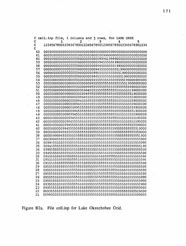
C cell. inp file, i columns and j rows, for LAKE OKEE C 1 2 · 3 4 5 C 123456789012345678901234567890123456789012345678901234 C

62 000000000000000000000000000000000000000000000000000000 61 000000000000000000000000000000099990000000000000000000 60 000000000000000000000000000009994199990000000000000000 59 000000000000000000000000000099455555199000000000000000 58 000000000000000000000000000994555555519990000000000000 57 000000000000000000000000000945555555555199000000000000 56 000000000000000000000000009955555555555519900000000000 55 000000000000000000000000099455555555555551990000000000 54 000000000000000000000000094555555555555555199000000000 53 000000000000000000000000995555555555555555519000000000 52 000000000000000000000099955555555555555555559990000000 51 000000000000000000000994555555555555555555555199000000 50 000000000000000000009945555555555555555555555519000000 49 000000000000000000999455555555555555555555555559000000 48 000000000000000009945555555555555555555555555559000000 47 000000000000000009455555555555555555555555555559000000 46 000000000000000099555555555555555555555555555559900000 45 000000000000000994555555555555555555555555555551900000 44 000000000000009945555555555555555555555555555555990000 43 000000000000099455555555555555555555555555555555190000 42 000000000000994555555555555555555555555555555555590000 41 000000000009945555555555555555555555555555555555599000 40 000000000099455555555555555555555555555555555555519000 39 000000009994555555555555555555555555555555555555559900 38 000009999455555555555555555555555555555555555555551900 37 000999455555555555555555555555555555555555555555555900 36 009945555555555555555555555555555555555555555555555990 35 009455555555555555555555555555555555555555555555555190 34 099555555555555555555555555555555555555555555555555590 33 094555555555555555555555555555555555555555555555555590 32 095555555555555555555555555555555555555555555555555590 31 095555555555555555555555555555555555555555555555555590 30 095555555555555555555555555555555555555555555555555590 29 095555555555555555555555555555555555555555555555555590 28 095555555555555555555555555555555555555555555555555590 27 095555555555555555555555555555555555555555555555555290 26 095555555555555555555555555555555555555555555555555990 25 095555555555555555555555555555555555555555555555555900 24 093555555555555555555555555555555555555555555555552900 23 099555555555555555555555555555555555555555555555559900 22 009355555555555555555555555555555555555555555555529000 21 009935555555555555555555555555555555555555555555599000

Figure B2a. File cell.inp for Lake Okeechobee Grid.

171

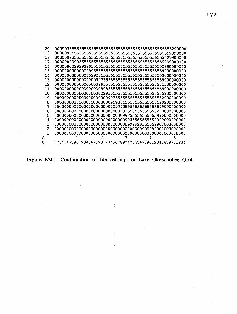
.20 000993555555555555555555555555555555555555555555290000 19 000099555555555555555555555555555555555555555552990000 18 000009935555555555555555555555555555555555555529900000 17 000000999355555555555555555555555555555555555299000000 16 000000009999999355555555555555555555555555552990000000 15 000000000000009935555555555555555555555555559900000000 14 000000000000000993555555555555555555555555559000000000 13 000000000000000099935555555555555555555555559900000000 12 000000000000000000993555555555555555555555551900000000 11 000000000000000000099355555555555555555555555900000000 10 000000000000000000009935555555555555555555555900000000

9 000000000000000000000999355555555555555555552900000000 8 000000000000000000000009993555555555555555529900000000 7 000000000000000000000000099935555555555555599000000000 6 000000000000000000000000000993555555555555290000000000 5 000000000000000000000000000099355555555555990000000000 4 000000000000000000000000000009935555555552900000000000 3 000000000000000000000000000000999999355559900000000000 2 000000000000000000000000000000000009999999000000000000 1 000000000000000000000000000000000000000000000000000000

C 1 2 3 4 5 C 123456789012345678901234567890123456789012345678901234

Figure B2b. Continuation of file cell.inp for Lake Okeechobee Grid.

172

PRCX;RAM GENGRID OPEN (1, FILE=' gridext. inp', S'I'ATUS= 'UNKNOWN') DO ~T=l, 62 DO I=l,54 X=FI.DAT ( I -1) Y=FI.DAT (J-1) WRI1:'E(l,100)I,J,X,Y END 00 END 00

100 FORt-1AT(2IS,2(2X,F12.3)) CLOSE (1) STOP END

Figure B4. FORTRAN program for generation of the gridext.inp file for the Lake Okeechobee grid shown in Figure B 1.

174

B.2. Kings Creek and Cherry Stone Inlet, Virginia

This section de:scribes a rectangular Cartesian grid of Kings Creek and Cherry Stone Inlet, located on the Eastern Shore of the Chesapeake Bay, north of Cape Charles, Virginia. The physical domain grid is shown in Figure BS, tht, cell.inp file in Figure B6, and the gefdc.inp file, Figure B7. The grid was generated with the NTYPE = 0, option by gefdc.f. The FORTRAN program for generation of the gridext.inp file ils shown in Figure B8.

175

-~ -

(.;:. ..... -'

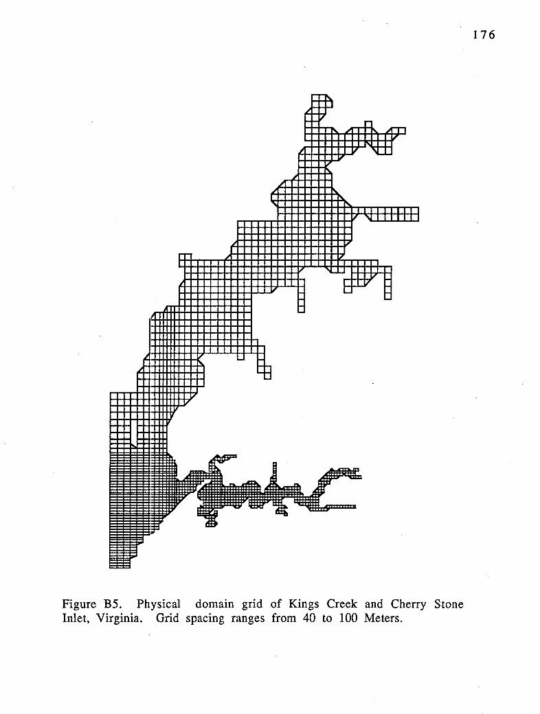
..-, -.... ..-,, I I I I r I ; ~tt / .,

" ... ~

,I ., .... I ' .... .....

I I I I I I I I I I i, '1 I I I I I I I

~ ., r- "

., I I I I

~ ~-U I I V -J c--./ -., .. -- --I -,,

" , - -' , I =a I

I ., .,

' - ...... -----.----

_I~ ---1 ~r -.. - ...... __a,,.

..., I Rf""" t cqmm ~ i ~ t --

i ~

~E~

Figure BS. Physical domain grid of Kings Creek and Cherry Stone Inlet, Virginia. Grid spacing ranges from 40 to 100 Meters.

176

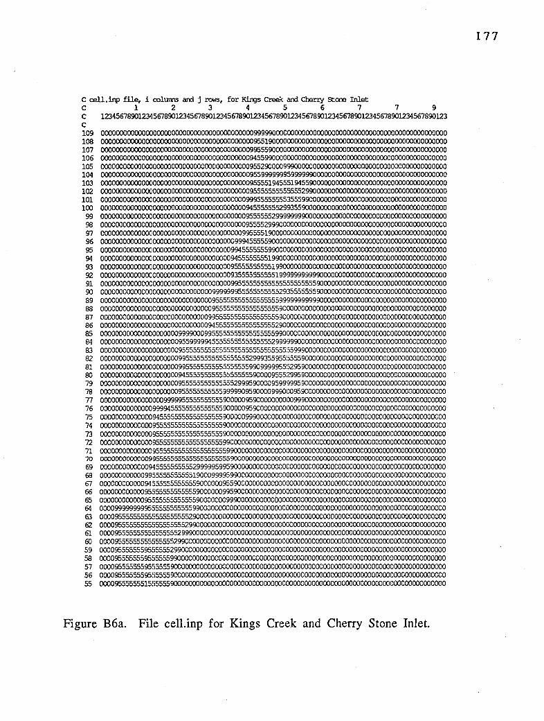
c cell.inp file, i colunns and j rows, for Kirgs Creek and Cherry Stone Inlet C 1 2 3 4 5 6 7 7 9 C 123456789012345678901234567890123456789012345678901234567890123456789012345678901234567890123 C 109 000000000000(X)0000000000000000000000000009999900000000000000000000000000000000000000000000000 108 000000000000CX)0000000000000000000000000009551900000000000000000000000000000000000000000000000 107 000000000000()()0000000000000000000000000099555900000000000000000000000000000000000000000000000 106 000000000000()()0000000000000000000000000094559900000000000000000000000000000000000000000000000 105 OOOOOOOOOOOOCXI0000000000000000000000000095529000099900000000000000000000000000000000000000000 104 OOOOOOOOOOOOOCI0000000000000000000000000095599999995999999000000000000000000000000000000000000 103 oooooooooooooc10000000000000000000000000095555194555194559000000000000000000000000000000000000 102 OOOOOOOOOOOOOCI0000000000000000000000000095555555555555299000000000000000000000000000000000000 101 oooooooooooooc10000000000000000000000000999555555553555990000000000000000000000000000000000000 100 0000000000000Cl()000000000000000000000000945555555299355900000000000000000000000000000000000000

99 oooooooooooooc10000000000000000000000000955555529999999900000000000000000000000000000000000000 98 oooooooooooooc,0000000000000000000000000955552999000000000000000000000000000000000000000000000 97 oooooooooooooc,0000000000000000000000009955551900000000000000000000000000000000000000000000000 96 OOOOOOOOOOOOOC10000000000000000000000999455555900000000000000000000000000000000000000000000000 95 oooooooooooooc,0000000000000000000009945555555990000000000000000000000000000000000000000000000 94 oooooooooooooc,0000000000000000000009455555555199000000000000000000000000000000000000000000000 93 000000000000000000000000000000000009555555555519900000000000000000000000000000000000000000000 92 000000000000000000000000000000000009355555555551999999999990000000000000000000000000000000000 91 000000000000000000000000000000000009955555555555555555555590000000000000000000000000000000000 90 000000000000000000000000000000999999955555555555293555555590000000000000000000000000000000000 89 000000000000000000000000000000955555555555555555999999999990000000000000000000000000000000000 88 000000000000000000000000000000955555555555555555900000000000000000000000000000000000000000000 87 000000000000000000000000000009955555555555555555900000000000000000000000000000000000000000000 86 000000000000000000000000000009455555555555555552900000000000000000000000000000000000000000000 85 000000000000000000000999900099555555555555555559900000000000000000000000000000000000000000000 84 000000000000000000000955999994555555555555555529999990000000000000000000000000000000000000000 83 000000000000000000000955555555555555555555555555555599900000000000000000000000000000000000000 82 000000000000C()0000000995555555555555555529993559555555900000000000000000000000000000000000000 81 00000000000000000000099555555555555555559909999955!5295900000000000000000000000000000000000000 80 000000000000000000000945555555555555555559000095552995900000000000000000000000000000000000000 79 000000000000000000000955555555555555299959000095999995900000000000000000000000000000000000000 78 000000000000000000000955555555555999990959000099900095900000000000000000000000000000000000000 77 000000000000000009999955555555555900000959000000000099900000000000000000000000000000000000000 76 000000000000009999455555555555555900000959000000000000000000000000000000000000000000000000000 75 000000000000009455555555555555555900000999000000000000000000000000000000000000000000000000000 74 000000000000.009555555555555555555900000000000000000000000000000000000000000000000000000000000 73 00000000000000955555555555555555590000000000000000C()00000000000000000000000000000000000000000 72 000000000000009555555555555555555990000000000000000000000000000000000000000000000000000000000 71 000000000000009555555555555555555599000000000000000000000000000000000000000000000000000000000 70 000000000000099555555555555555555559000000000000000000000000000000000000000000000000000000000 69 000000000000094555555555529999959959000000000000000000000000000000000000000000000000000000000 68 000000000000995555555555519000999959900000000000000000000000000000000000000000000000000000000 67 000000000000945555555555559000000955900000000000000000000000000000000000000000000000000000000 66 000000000000955555555555559000000995900000000000000000000000000000000000000000000000000000000 65 000000000000955555555555559000000099900000000000000000000000000000000000000000000000000000000 64 000099999999955555555555599000000000000000000000000000000000000000000000000000000000000000000 63 000095555555555555555555290000000000000000000000000000000000000000000000000000000000000000000 62 000095555555555555555552990000000000000000000000000000000000000000000000000000000000000000000 61 000095555555555555555299900000000000000000000000000000000000000000000000000000000000000000000 60 000095555555555555552990000000000000000000000000000000000000000000000000000000000000000000000 59 000095555555955555529900000000000000000000000000000000000000000000000000000000000000000000000 58 000095555555955555599000000000000000000000000000000000000000000000000000000000000000000000000 57 00009555555595!;555590000000000000000000000000000000000000000000000000000000000000000000000000 56 000095555555955555590000000000000000000000000000000000000000000000000000000000000000000000000 55 000095555555155555590000000000000000000000000000000000000000000000000000000000000000000000000

Figure B6a. File cell.inp for Kings Creek and Cherry Stone Inlet.

177

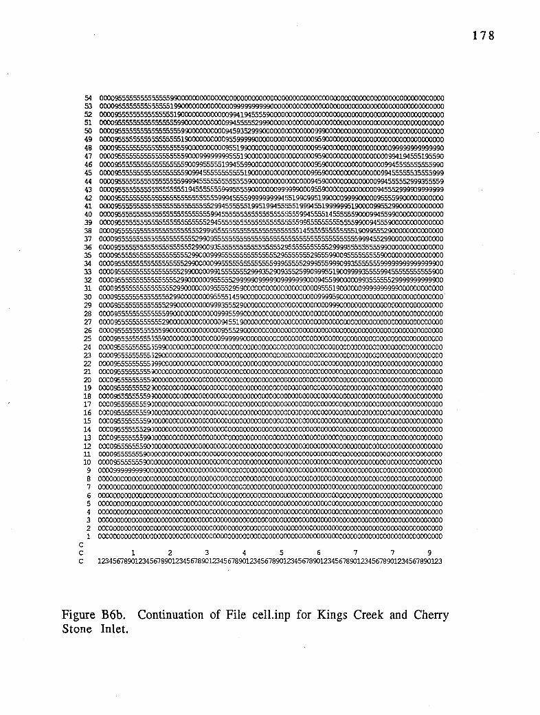
C

54 000095555555555555599000000000000000000000000000000000000000000000000000000000000000000000000 53 000095555555555555519900000000000000999999999900000000000000000000000000000000000000000000000 52 000095555555555555551900000000000009941945555900000000000000000000000000000000000000000000000 51 000095555555555555555990000000000099455555299900000000000000000000000000000000000000000000000 50 000095555555555555555599000000000094593529990000000000000099900000000000000000000000000000000 49 000095555555555555555519000000000095599999000000000000000095900000000000000000000000000000000 48 000095555555555555555559000000000095519900000000000000000095900000000000000000099999999999990 47 000095555555555555555559000999999995551900000000000000000095900000000000000000994194555195590 46 000095555555555555555559009955555199455990000000000000000095900000000000000009945555555555990 45 000095555555555555555559099455555555555190000000000000000995900000000000000099455555535555999 44 000095555555555555555599994555555555555590000000000000000945900000000000000994555552999355559 43 000095555555555555555551945555555999555590000000999999000955900000000000000945552999909999999 42 000095555555555555555555555555559994555599999999945519909951990000999900000955559900000000000 41 000095555555555555555555555555299455555519951994555551999455199999951900009955299000000000000 40 000095555555555555555555555555994555555555555555555555994555514555555900099455990000000000000 39 00009555555555.5555555555555552945555555555555555555555995555555555555990094555900000000000000 38 00009555555555:555555555555529995555555555555555555!5555145555555555555190995552900000000000000 37 00009555555555555555555555299095555555555555555555!5555555555555555555599945529900000000000000 36 00009555555555.5555555555529900935555555555555555529555555555552999955555555599000000000000000 35 00009555555555555555555529900099955555555555555529!5555555295559900955555555590000000000000000 34 00009555555555.555555555299000009955555555555555999!5555529995559990993555555599999999999999900 33 000095555555555555555529900000991555555529993529093552599099955190099993555599455555555555900 32 000095555555555555555299000000955555299999099999099999990009455990000099355555529999999999900 31 000095555555555555552990000000955552959000000000000000000009555190000009999999999000000000000 30 000095555555555555529900000000955551459000000000000000000009999590000000000000000000000000000 29 000095555555555555299000000000999355529000000000000000000000009990000000000000000000000000000 28 000095555555555555990000000000009995599000000000000000000000000000000000000000000000000000000 27 000095555555555552900000000000000945519000000000000000000000000000000000000000000000000000000 26 000095555555555559900000000000000955529000000000000000000000000000000000000000000000000000000 25 000095555555555559000000000000000999999000000000000000000000000000000000000000000000000000000 24 000095555555555599000000000000000000000000000000000000000000000000000000000000000000000000000 23 000095555555555290000000000000000000000000000000000000000000000000000000000000000000000000000 22 000095555555559990000000000000000000000000000000000000000000000000000000000000000000000000000 21 000095555555559000000000000000000000000000000000000000000000000000000000000000000000000000000 20 000095555555559000000000000000000000000000000000000000000000000000000000000000000000000000000 19 000095555555529000000000000000000000000000000000000000000000000000000000000000000000000000000 18 00009555555559900000000000000000000000000000000000()000000000000000000000000000000000000000000 17 000095555555590000000000000000000000000000000000000000000000000000000000000000000000000000000 16 000095555555590000000000000000000000000000000000000000000000000000000000000000000000000000000 15 000095555555590000000000000000000000000000000000000000000000000000000000000000000000000000000 14 00009555555529000000000000000000000000000000000000()000000000000000000000000000000000000000000 13 000095555555990000000000000000000000000000000000000000000000000000000000000000000000000000000 12 000095555555900000000000000000000000000000000000000000000000000000000000000000000000000000000 11 000095555555901)000000000000000000000000000000000000000000000000000000000000000000000000000000 10 00009555555590000000000000000000000000000000000000()000000000000000000000000000000000000000000 9 000099999999900000000000000000000000000000000000000000000000000000000000000000000000000000000 8 000000000000000000000000000000000000000000000000000000000000000000000000000000000000000000000 7 000000000000000000000000000000000000000000000000000000000000000000000000000000000000000000000 6 000000000000000000000000000000000000000000000000000000000000000000000000000000000000000000000 5 000000000000000000000000000000000000000000000000000000000000000000000000000000000000000000000 4 000000000000000000000000000000000000000000000000000000000000000000000000000000000000000000000 3 000000000000000000000000000000000000000000000000000000000000000000000000000000000000000000000 2 000000000000000000000000000000000000000000000000000000000000000000000000000000000000000000000 1 000000000000000000000000000000000000000000000000000000000000000000000000000000000000000000000

C 1 2 3 4 5 6 7 7 9 C 123456789012345678901234567890123456789012345678901234567890123456789012345678901234567890123

Figure B6b. Continuation of File cell.inp for Kings Creek and Cherry Stone Inlet.

178

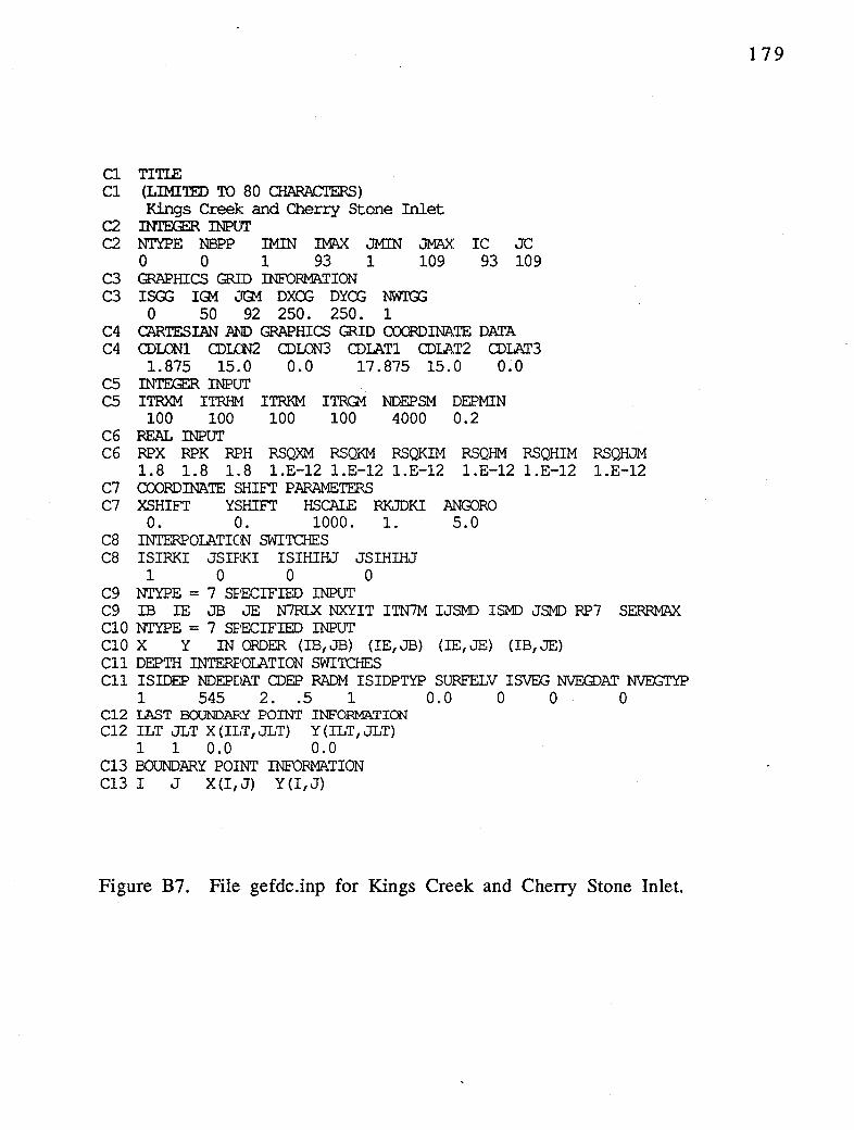
Cl TITIE Cl (LIMI'IED TO 80 OiARACTERS)

Kings Creek and Cherry Stone Inlet C2 INl'EGSR INPtrr C2 NTYPE NBPP !MIN IMAX JMIN JMAX IC JC

0 0 1 93 1 109 93 109 C3 GRAPHICS GRJD INFORMATION C3 ISGG IG1 ~fQ.1 DXCG DYCG NWlGG

0 50 92 250. 250. 1 C4 CAR'IESIAN AND GRAPHICS GRID COORDINATE DATA C4 Q)I.ON1 Q)L(N2 Q)I.0N3 Q)IATl Q)LAT2 Q)LAT3

1.875 15.0 0.0 17.875 15.0 0.0 CS INl'EGSR INPtrr CS ITRXM ITRHM ITRKM ITRG1 NDEPSM DEPMIN


1.8 1.8 1.8 1.E-12 l.E-12 1.E-12 1.E-12 1.E-12 1.E-12 C7 COORDINATE SHIFT PARAMETERS C7 XSHIFT YSHIFT HSCAIB RKJDKI ANGORO

o. Cl. 1000. 1. 5.0 ca INTERPOLATION SWITCHES C8 ISIRKI JSIRKI ISIHIHJ JSIHIHJ

1 0 0 0 C9 NTYPE = 7 SPECIFIED INPUT C9 IB IE JB JE N7RLX NXYIT ITN7M IJSMD ISMD JSMD RP7 SERRMAX ClO NTYPE = 7 SPECIFIED INPUT ClO X Y IN ORDER (IB, JB) (IE, JB) (IE, JE) (IB, JE) Cll DEPTH INTERPOLATION SWITCHES Cll ISIDEP NDEPDAT Q)EP RADM ISIDPTYP SURFELV ISVEG NVEGDAT NVEGTYP

1 545 2 .. 5 1 0.0 0 0 0 C12 LAST BOUNDARY POINT INFORMATION Cl2 ILT JLT X(ILT,JLT) Y(ILT,JLT)

1 1 0.0 0.0 Cl3 BOUNDARY POINT INFORMA.TION Cl3 I J X(I,J) Y(I,J)

Figure B7. File gefdc.inp for Kings Creek and Cherry Stone Inlet.

179

C

C

C

C

C

C

C

PRCXiRAM GVARCGRID

DIMENSION X(93,109},Y(93,109}

00 ~T=l,53 00 I=l,93 Y(I,J}=40.*FLOAT(J}+630. END 00 END 00

00 I=l,93 Y(I,54}=2800. Y(I,55}=2860. Y(I,56}=2930. Y(I,57}=3010. END 00

00 ~r=S8, 109 00 I=l,93 Y (I, J} =100. *FLOAT (J-58} +3100. END 00 END 00

00 ,.J=l, 109 00 I=l,14 X(I,J)=l00.*F1.0AT(I) END 00 X(l5,J)=l490. X(l6,J)=l580. X(l7,J)=l660. X(l8,J)=l730. X(l9,J)=l790. X(20,J)=l840. END 00

00 J;=l,54 00 I=21,93 X (I, J} =40. *F1.0AT (I-21) + 1880. END 00 END 00

00 J·=sS, 109 X(21,J)=l890. X(22,J)=l950. X(23,J)=2020. 00 I=24,93 X (I, J} =100. *FLOAT (I-24) +2100. END 00 END 00

Figure B8a. FORTRAN program for generation of gridext.inp file.

180

C

C

C

OPEN (1, FILE=' gridext. inp', STATUS= 'UNKNOWN') DO ~T=l, 109 DO I=l,93 X (I,. J) = (X (I, J) /1000.) +408. Y (I,J) =(Y (I,J) /1000.) +124. WRI"Jl"E(l,20) I,J,X(I,J), Y(I,J) END DO END DO CLOSE (1)

OPEN (1, FILE=' rnaskij. dat' , STATUS=' UNKNOWN' ) OPEN (2, FILE=' shorernask' , STATUS=' UNKNOWN' ) OPEN (3, FILE=' shoredep' , STA'ruS= 'UNKNOWN') DEP==0.1 DO N=l,337 READ(l,*)J,I WRI1E(2,2000)X(I,J),Y(I,J) IF (I.NE. 6.0R.J.NE.10) THEN

WFtITE(3,3000)X(I,J),Y(I,J),DEP XTMl?=X(I,J)+.01 YTMl?=Y(I,J)+.01 WFtITE (3, 3000) X (I, J), YTMP ,DEP WFtITE (3, 3000) XTMJ?, Y (I, J), DEP XTMP=X (I, J) - . 01 YTMl?=Y(I,J)-.01 WFtITE (3, 3000) X (I, J) , YTMP, DEP WFtITE (3, 3000) XTMJ?, Y (I, J), DEP

END IF END DO CLOSE (1) CLOSE (2) CLOSE (3)

20 FORMAT(2I5,2X,F12.6,2X,Fl2.6) 2000 FO~IA.T(2X,Fl2.6,2X,Fl2.6) 3000 FO~!AT(2X,F12.6,2X,F12.6,2X,F6.2)

C STOP END

C

Figure B8b. Continuation of FORTRAN program for generation of gridext.inp file.

181

B.3. Rose Bay, Florida

This section de:scribes a curvilinear orthogonal grid of Rose Bay, on the Halifax River, near New Smyrna Beach, Florida. The physical domain grid is shown in Figure B9, the cell.inp file in Figure B 10, and the gefdc.inp file in Figure B 11. The grid was generated with the NTYPE = 5, option by gefdc.f.

Figure B9. Physical domain grid of Rose Bay, Florida. Grid spacing ranges between approximately 20 and 90 meters.

182

C cell. inp file, i columns and j rows, for Rose Bay C 1 2 3 4 5 C 12345678901234567890123456789012345678901234567890 C

C

25 00000000000000000000000000000000000000000000000000 24 00000000000000000000000000000000000000000000000000 23 00000000000000000000000000000000000000000000000000 22 00000009990000000000000000000000000000000000000000 21 00000009590000000000000000000000000000000000099900 20 00000009590999900000000000000000000000000000095900 19 00000009590914900000000000000000000000000000095900 18 00999999599955999999999999999999999999999999995900 17 00955555599455514555555555555555555555555555555900 16 00999955599555555555555555555555555555555555555900 15 00009555599555555555555555555555555555555555555900 14 00009555599555555555555555555555555555555555555900 13 00009555599555555555555555555555555555555555555900 12 00009325555555555555555555555555555555555555555900 11 00009995555555555555555523555555555555555555552900 10 00000099999999999999999999999999999999955555551900

9 00000000000000000000000000000000000009555555555,999 8 00000000000000000000000000000000000009555555535559 7 00000000000000000000000000000000000009555555599999 6 00000000000000000000000000000000000009555555590000 5 00000000000000000000000000000000000009999999990000 4 00000000000000000000000000000000000000000000000000 3 00000000000000000000000000000000000000000000000000 2 00000000000000000000000000000000000000000000000000 1 00000000000000000000000000000000000000000000000000

C 1 2 3 4 5 C 12345678901234567890123456789012345678901234567895

Figure BlO. File cell.inp for Rose Bay.

183

Cl TITIE Cl (LIMI'IED TO 80 OIARACTERS)

rose bay C2 IN'I'EraR INPUT C2 NTYPE NBPP IMIN IMAX JMIN JMAX IC JC

S 148 1 so 1 25 50 25 C3 GRAPHICS GRID INFOFMA.TION C3 ISGG IG1 ~TG1 DXCG DYCG NWTGG

0 96 180 1850. 1850. 1 C4 CARTESIAN AND GRAPHICS GRID COORDINATE DATA C4 CDWNl cou:m CDWN3 CDIATl CDIAT2 CDIAT3

-77.5 1.25 -0.625 36.7 1.0 -0.5 CS IN'I'EraR INPUI' CS ITRXM ITRHM ITRKM ITRG1 NDEPSM DEPMIN


1.8 1.8 1.8 l.E-12 1.E-12 l.E-12 l.E-12 l.E-12 l.E-12 C7 COORDINATE SHIFI' PARAMETERS C7 XSHIFT YSHIFT HSCAI.E RK.JDKI ANGORO

0. o. 1. 1. 9.0 ca INTERPOIATION SWITCHES ca ISIRKI JSIRKI ISIHIHJ JSIHIHJ

1 0 0 0 C9 NTYPE = 7 SPECIFIED INPUT C9 IB IE JB JE N7RLX NXYIT ITN7M IJSMD ISMD JSMD RP7 SERRMAX ClO NTYPE = 7 SPECIFIED INPUT ClO X Y IN ORDER (IB, JB) (IE, JB) (IE, JE) (IB, JE) Cll DEPTH INTER.POIATION SWITCHES Cll ISIDEP NDEPDAT CDEP RADM ISIDPTYP SURFELV ISVEG NVEGDAT NVEGTYP

1 62 2 .. 5 1 5.0 0 0 0 Cl2 LAST BOONDARY POINT INFORMATION Cl2 ILT JLT X(ILT,JLT) Y(ILT,JLT)

40 6 1456. 16. C13 BOUNDARY POJNI' INFORMATION Cl3 I J X(I,J) Y(I,J)

39 6 1440.000 39 7 1420.000 39 8 1400.000 39 9 1380.000 39 10 1356.000 40 10 1372.000 40 11 1340.000 39 11 1308.480 38 11 1270.640 37 11 1218.480

0.000 20.000 40.000 60.000 84.000

100.000 132.000 112.080 89.200 60.400

Figure Blla. File gefdc.inp for Rose Bay.

184

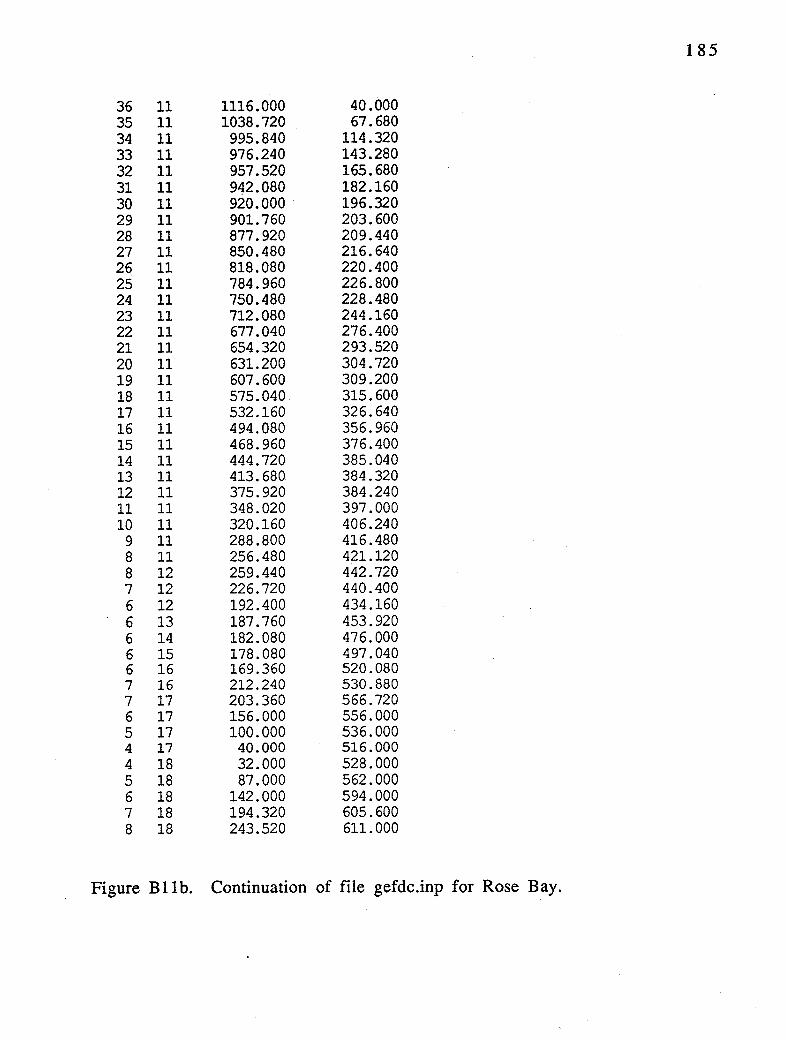
185

36 11 1116.000 40.000 35 11 1038.720 67.680 34 11 995.840 114.320 33 11 976.240 143.280 32 11 957.520 165.680 31 11 942.000 182.160 30 11 920.000 196.320 29 11 901.760 203.600 28 11 877.920 209.440 27 11 850.480 216.640 26 11 818.080 220.400 25 11 784.960 226.800 24 11 750.480 228.480 23 11 712.080 244.160 22 11 677.040 276.400 21 11 654.320 293.520 20 11 631.200 304.720 19 11 607.600 309.200 18 11 575.040 315.600 17 11 532.160 326. 640 16 11 494.080 356.960 15 11 468.960 376.400 14 11 444.720 385.040 13 11 413.680 384.320 12 11 375.920 384.240 11 11 348.020 397.000 10 11 320.160 406.240

9 11 288.800 416.480 8 11 256.480 421.120 8 12 259.440 442.720 7 12 226.720 440.400 6 12 192.400 434.160 6 13 187.760 453.920 6 14 182.080 476.000 6 15 178.080 497.040 6 16 169.360 520.080 7 16 212.240 530.880 7 17 203.360 566.720 6 17 156.000 556.000 5 17 100.000 536.000 4 17 40.000 516.000 4 18 32.000 528.000 5 18 87.000 562.000 6 18 142.000 594.000 7 18 194.320 605.600 8 18 243.520 611.000

Figure Bllb. Continuation of file gefdc.inp for Rose Bay.

186

9 18 280.000 611.000 9 19 290.000 660.000 9 20 294.000 710.000 9 21 280.000 760.000 9 22 280.000 800.000

10 22 320.000 800.000 10 21 320.000 760.000 10 20 320.000 710.000 10 19 310.000 660.000 10 18 312.000 610.000 10 17 315.440 573.680 10 16 321.840 547.200 10 15 331.440 516.880 10 14 338.800 487.040 10 13 336.480 456.960 11 13 362.960 447.280 12 13 384.560 442.880 12 14 389.120 473.280 12 15 396.720 504.720 12 16 408.320 538.480 12 17 423.920 567.040 12 18 441.600 598.960 13 18 475.000 585.000 13 19 492.000 612.000 13 20 520.000 647.000 14 20 540.000 640.000 15 20 560.000 633.000 15 19 552.000 590.000 15 18 547.000 564.000 16 18 575.920 559.360 17 18 605.520 558.400 18 18 644.800 557.360 19 18 689.200 558.000 20 18 734.800 551.120 21 18 773.280 536.080 22 18 812.560 512.800 23 18 840.080 493.440 24 18 866.880 470.800 25 18 891. 920 447.920 26 18 915.920 422.080 27 18 941.200 399.840 28 18 967.200 386.160 29 18 998.400 378.960 30 18 1038.000 366.880 31 18 1066.320 348.640 32 18 1088.480 326.880

Figure B llc. Continuation of file gefdc.inp for Rose Bay.

187

33 18 1107.040 302.640 34 18 1124.320 285.680 35 18 1144.560 272.320 36 18 1162.480 264.800 37 18 1182.800 260.560 38 18 1204.640 266.640 39 18 1224.720 284.400 40 18 1240.640 298.880 41 18 1265.440 316.240 42 18 1289.040 333.440 43 18 1311.280 348.960 44 18 1332.960 360.480 45 18 1356.800 372.560 46 18 1379.280 388.240 47 18 1403.000 404.000 47 19 1380.000 440.000 47 20 1355.000 475.000 47 21 1326.000 512.000 48 21 1340.000 520.000 48 20 1370.000 485.000 48 19 1395.000 455.000 48 18 1425.920 422.800 48 17 1444.000 401.120 48 16 1460.880 379.840 48 15 1477.200 349.440 48 14 1488.240 320.480 48 13 1494.800 293.040 48 12 1501.680 272.640 48 11 1512.560 253.920 48 10 1528.400 235.040 48 9 1540.000 220.000 49 9 1560.000 240.000 50 9 1580.000 260.000 50 8 1600.000 240.000 49 8 1580.000 220.000 48 8 1560.000 200.000 47 8 1540.000 180.000 46 8 1520.000 160.000 46 7 1540.000 140.000 46 6 1560.000 120.000 45 6 1541.000 101.000 44 6 1523.000 83.000 43 6 1505.500 65.500 42 6 1488.500 48.500 41 6 1470.000 32.000 40 6 1456.000 16.000

Figure B 11 d. Continuation of file gefdc.inp for Rose Bay.

B.4. Indian River Lagoon, Florida

This section describes the construction of a composite grid of a section of the Indian River Lagoon, near Melborne, Florida, from five subgrids. Figures B 12-B 14 show the composite grid, and the corresponding cell.inp and gefdc.inp files. The composite grid was generated with the NTYPE = 0 option by gefdc.f. The input file, gridext.inp, specifying the composite grid was formed by combining the five gridext.out files generated for the five subgrid regions. Figure Bl5&Bl6, B17&Bl8, B19&B20, B21&B22, and B23&B24 show the subgrids and the corresponding gefdc.inp files. The cell.inp file for each sub grid is similar to the cell.inp file shown in Figure B 13, with only the water cells in the particular subgrid activated. The first sub grid, Figures B 15&B 16, and the fourth subgrid, Figure B21&B22, were generated with the NTYPE = 0 option. The remaining subgrids are curvilinear-orthogonal and were generated with the NTYPE = 5 option.

188

189

Figure B12. Grid of a section of the Indian River Lagoon near Melbourne, FL. Grid is a composite of five subgrids.

C cell.inp file, i columns and j rows, for Indian River Lag C 1 2 3 4 5 C 123456789012345678901234567890123456789012345678901234 C

60 000000000000000000000000000000000999999999999999999900 59 000000000000000000000000000000000955555555555555555990 58 000000000000000000000000000000000955555555555555555190 57 000000000000000000000000000000000935555555555555555590 56 000000000000000000000000000000000993555555555555555590 55 000000000000000000000000000000000959955555555555555590 54 000000000000000000000000000000000955555555555555555590 53 000000000000000000000000000000000955555555555555555290 52 000000000000000000000000000000000955555555555555555190 51 000000000000000000000000000000000935555555555555555590 50 000000000000000000000000000000000995555555555555555590 49 000000000000000000000000000000000995555555555555555590 48 000000000000000000000000000000009945555555555555555590 47 000000000000000000000000000000009455555555555555555290 46 000000000000000000000000000000009555555555555555555990 45 000000000000000000000000000000009555555555555555555190 44 000000000000000000000000000000009355555555555555555590 43 000000000000000000000000000000009935555555555555555590 42 000000000000000000000000000000000995555555555555555590 41 000000000000000000000000000000000093555555555555555590 40 000000000000000000000000000000999994555555555555555590 39 000000000000000000000000000000945555555555555555555590 38 000000000000000000000000000000955555555555555555555590 37 000000000000000000000000000000955523555555555555555590 36 000000000000000000000000000999955299555555555555555590 35 000000000000000999999999999955959999555555555555555590 34 000000000000000955555555555555559094555555555555555590 33 000000000000000959599995555952999995555555555555555590 32 000000000000000959595555552959900945555555555555555290 31 000000000000000959599999999939009955555555555555555190 30 000000000000000959590000000999009455555555555555555590 29 009999999000000959590000000000009355555555555555555590 28 009559959999999959590000000000009935555555555555555599 27 009555555555555555590000000000009999455555555555555519 26 009599999959599999990000000000009455555555555555555559 25 999590000959590000000000000000009555555555555555555559 24 955590000959590000000000000000009355555555555555555529 23 999990000999590000000000000000009955555555555555555599 22 000000000009590000000000000000009955555555555555555519 21 000000000009590000000000000000009455555555555555555559

Figure B 13a. File cell.inp for the Indian River Lagoon grid shown m Figure B12.

190

20 000000000009990000000000000000009555555555555555555529 19 000000000000000000000000000000009355555555555555555519 18 000000000000000000000000000000009935555555555555555559 17 000000000000000000000000000000000995555555555555555559 16 000000000000000000000000000000000095555555555555555299 15 000000000000000000000000000000000095555555555555555990 14 000000000000000000000000000000000093555555555555555490 13 000000000000000000000000000000000099955555555555555599 12 000000000000000000000000000000000000935555555555555519 11 000000000000000000000000000000000000993555555555555559 10 000000000000000000000000000000000000999555555555555559

9 000000000000000000000000000000000000009555555555555559 8 000000000000000000000000000000000000009555555555555529 7 000000000000000000000000000000000000009555555555555519 6 000000000000000000000000000000000000009555555555555559 5 000000000000000000000000000000000000009555555555555559 4 000000000000000000000000000000000000009555555555555539 3 000000000000000000000000000000000000009555555555555299 2 000000000000000000000000000000000000009555555555555990 1 000000000000000000000000000000000000009999999999999900

Figure B13b. Continuation of File cell.inp for the Indian River Lagoon grid shown in Figure B 12.

191

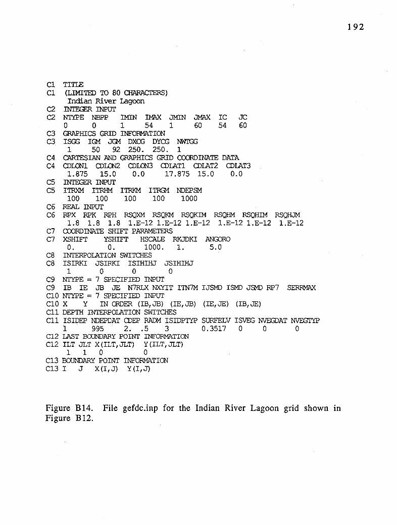
Cl TITIE Cl (LIMITED TO 80 rnARACTERS}

Indian Ri ve:r lagoon C2 INTEGER INPUT C2 NTYPE NBPP IMIN IMAX JMIN ~ IC JC

0 0 1 54 1 60 54 60 C3 GRAPHICS GRID INFORMATION C3 ISGG IG1 JG1 DXCG DYCG NWIGG

1 50 92 250. 250. 1 C4 CARTESIAN AND GRAPHICS GRID COORDINATE DATA C4 CDLONl CDLCN2 CDLON3 COLA.Tl CDLA.T2 CD1AT3

1.875 15.0 0.0 17.875 15.0 0.0 CS INTEGER INPUT CS ITRXM I~[ ITRKM ITRG1 NDEPSM

100 100 100 100 1000 C6 REAL INPUT C6 RPX RPK RPH RSQXM RSQKM RSQKIM RSQHM RSQHIM RSQHJM

1.8 1.8 1.8 1.E-12 1.E-12 1.E-12 1.E-12 1.E-12 1.E-12 C7 COORDINATE SHIFT PARAMETERS C7 XSHIFT YSHIFT HSCAI.E RKJDKI ANGORO

0. 0. 1000. 1. 5.0 CS INI'ERPOLA.TION SWITCHES CS ISIRKI JSIRKI ISIHIHJ JSIHIHJ

1 0 0 0 C9 NTYPE = 7 SPECIFIED INPUT C9 IB IE JB JE N7RLX NXYIT ITN7M IJSMD ISMD JSMD RP7 SERRMAX ClO NTYPE = 7 SPECIFIED INPUT ClO X Y IN ORDER (IB,JB) (IE,JB} (IE,JE) (IB,JE) Cll DEPTH INI'ERPOLA.TION SWITCHES Cll ISIDEP NDEPDAT CDEP RADM ISIDPTYP SURFELV ISVEG NVEGDAT NVEGTYP

1 995 2 .. 5 3 0.3517 0 0 0 Cl2 LAST BCUNDARY POINT INFORMATION Cl2 ILT JLT X ( ILT, JLT) Y ( ILT, JLT}

1 1 0 0 Cl3 BOUNDARY POINT INFORMATION C13 I J X(I,J) Y(I,J}

Figure B 14. File gefdc.inp for the Indian River Lagoon grid shown m Figure B12.

192

Figure Bl5. Subgrid 1 of the Indian River Lagoon grid shown in Figure B 12. This grid is a variable spacing Cartesian grid generated with NTYPE = 0, option by gefdc.f.

193

Cl TITIE Cl (LIMITED TO 80 OIARACTERS)

Indian River Lagoon, sub grid 1 C2 IN'IEGER INPUT C2 NTYPE NBPP IMIN IMAX JMIN JMAX IC JC

0 146 1 54 1 60 54 60 C3 GRAPHICS GRID INFORMATION C3 ISGG IG1 J"Q.1 DXCG DYCG NWTGG

0 50 92 250. 250. 1 C4 CARTESIAN AND GRAPHICS GRID COORDINATE DATA C4 CDLONl CDLCN2 CDI.0N3 CDIATl CDIAT2 CDIAT3

1.875 15.0 0.0 17.875 15.0 0.0 C5 IN'IEGER INPUT C5 ITRXM ITRHM ITRKM ITRGM NDEPSM


1.8 1.8 1.8 1.E-12 1.E-12 l.E-12 1.E-12 1.E-12 l.E-12 C7 COORDINATE SHIFT PARAMETERS C7 XSHIFT YSHIFT HSCALE RKJDKI ANGORO

0. 0. 1000. 1. 1.0 ca INTERPOIATICN SWITCTJES CS ISIRKI JSIFKI ISIHIHJ JSIHIHJ

0 0 1 0 C9 NTYPE = 7 SPECIFIED INPUT C9 IB IE JB JE N7RLX NXYIT ITN7M IJSMD ISMD JSMD RP7 SERRMAX ClO NTYPE = 7 SPECIFIED INPUT ClO X Y IN ORDER (IB, JB) (IE, JB) (IE, JE) (IB, JE) Cll DEPTH INTERPOLATION SWITCTJES Cll ISIDEP NDEPDAT CDEP RADM ISIDPTYP SURFELV ISVEG NVEQ)AT NVEGTYP

0 896 2 .. 5 3 0.35 0 0 0 C12 IAST BCX.JNDARY POINT INFORMATION Cl2 !LT JLT X(ILT,JLT) Y(ILT,JLT)

0 0 0.0 0.0 C13 BOUNDARY POINT INFORMATION Cl3 I J X(I,J) Y(I,J)

Figure B16. File gefdc.inp for subgrid 1, shown in Figure B15.

194

[

Figure B17. Figure BIO. NTYPE=5.

Subgrid 2 of the Indian River Lagoon grid shown in This grid is a curvilinear-orthogonal grid generated with

195

Cl TITIB Cl (LIMITED TO 80 CHARACTERS)

Indian Ri veir Lagoon, Subgrid 2 C2 INTEC?ER INPUI' C2 NTYPE NBPP IMIN IMAX JMIN JMAX IC JC

5 140 1 54 1 60 54 60 C3 GRAPHICS GRID INFORMATION C3 ISGG IGi .:rGM DXCG DYCG NWI'GG

0 50 92 250. 250. 1 C4 CARTESIAN ,N;[) GRAPHICS GRID COORDINATE DATA C4 CT>I.DNl CT>U:N2 CT>I.DN3 CT>IATl CT>IAT2 CT>IAT3

1.875 15.0 0.0 17.875 15.0 0.0 CS INTEC?ER INPU~' CS ITRXM ITRHM ITRKM ITRQ1 NDEPSM


1.8 1.8 1.8 1.E-12 1.E-12 1.E-12 1.E-12 1.E-12 1.E-12 C7 COORDINATE SHIFT PARAMETERS C7 XSHIFT YSHIFT HSCALE RKJDKI ANGORO

0. 0. 1000. 1. 10.0 ca INTERPOIATICN SWITCHES ca ISIRKI JSIF:KI ISIHIHJ JSIHIHJ

1 0 0 0 C9 NTYPE = 7 SPECIFIED INPUT C9 IB IE JB JE N7RLX NXYIT I'IN7M IJSMD ISMD JSMD RP7 SERRMAX ClO NTYPE = 7 SPECIFIED INPUT ClO X Y IN ORDER (IB, JB) (IE, JB) (IE, JE) (IB, JE) Cll DEPTH INTERPOIATION SWITCHES Cll ISIDEP NDEPDAT CT>EP RADM ISIDPTYP SURFELV ISVEG NVEGDAT NVEGTYP

0 1054 2 .. 5 3 0.167 0 0 0 Cl2 LAST BOONDARY POINI' INFORMATION C12 ILT JLT X(ILT,JLT) Y(ILT,JLT)

36 39 5.416584 32.868687 C13 BOUNDARY POlNT INFORMATION C13 I J X(I,J) Y(I,J)

36 38 5.458846 32.778057 36 37 5.501108 32.687428 35 37 5.446730 32.662067 35 36 5.514679 32.611004 34 36 5.459079 32.540939 33 36 5.396529 32.462120 33 35 5.468399 32.390812 33 34 5.520639 32.337936 32 34 5.476520 32.278748

Figure B 18a. File gefdc.inp for sub grid 2, shown in Figure B 17.

196

31 34 5.403405 32.222584 31 33 5.452924 32.151886 30 33 5.364405 32.105095 30 32 5.395795 32.025944 30 31 5.452544 31.892416 29 31 5.370976 31.854382 29 32 5.312114 31.992439 29 33 5.276192 32.069473 29 34 5.239964 32.135338 28 34 5.165042 32.094883 28 33 5.199157 32.033554 28 32 5.235079 31.956518 27 32 5.148980 31. 916368 26 32 5.060462 31. 869576 25 32 4.971944 31.822783 24 32 4.878895 31.773876 23 32 4.790073 31.715906 22 32 4.664386 31.618679 21 32 4.537784 31.487925 21 33 4.500639 31.520256 22 33 4.625128 31.655542 23 33 4.762297 31.763639 24 33 4.846588 31.819498 24 34 4.818812 31.867229 23 34 4.725458 31.807148 22 34 4.636329 31.738003 21 34 4.549620 31. 675501 20 34 4.440557 31.613609 20 33 4.451099 31.508188 20 32 4.437174 31.407907 20 31 4.415995 31.287693 20 30 4.396928 31.162949 20 29 4.373633 31.047266 20 28 4.360015 30.948162 20 27 4.355037 30.905406 19 27 4.318927 30.908500 18 27 4.269384 30.905899 17 27 4.226488 30.901413 16 27 4.189625 30.862158 15 27 4.145506 30.802967 14 27 4.103806 30.750420 14 26 4.131277 30.691509 14 25 4.207983 30.633492 14 24 4.287153 30.627129 14 23 4.375015 30.606558

Figure B18b. Continuation of file gefdc.inp for subgrid 2, shown in Figure B17.

197

14 22 4.447190 30;546427 14 21 4.496096 30.453379 13 21 4.473438 30.442812 13 22 4.424227 30.524685 13 23 4.358696 30.582397 13 24 4.280768 30.595711 13 25 4.198070 30.602991 13 26 4.103477 30.656477 13 27 4.043370 30.667067 12 27 3.989883 30.592476 12 26 4.019771 30.540209 12 25 4.100399 30.461952 12 24 4.158063 30.361954 11 24 4.135406 30.351387 11 25 4.086499 30.444435 11 26 3.996809 30.518467 11 27 3.945765 30.533283 10 27 3.894697 30.465336 9 27 3.830034 30.391047 8 27 3.734261 30.324322 7 27 3.626115 30.295958 6 27 3.518578 30.289949 5 27 3.425249 30.312630 5 26 3.393198 30.203899 5 25 3.376549 30.085796 5 24 3.377136 30.025385 4 24 3.339077 30.024187 3 24 3.133373 30.027571 2 24 2.909850 30.033678 2 25 2.909263 30.094091 3 25 3.128256 30.085871 4 25 3.345134 30.082182 4 26 3.362088 30.211458 4 27 3.392026 30.324722 4 28 3.397473 30.360365 4 29 3.414402 30.406878 5 29 3.451852 30.390721 6 29 3.531892 30.367876 6 28 3.521913 30.330122 7 28 3.629143 30.324955 8 28 3.723696 30.346979 8 29 3.711017 30.374166 9 29 3.775374 30.437279 9 28 3.805872 30.407366

10 28 3.863892 30.484074 11 28 3.919492 30.554134

Figure B 18c. Continuation of file gefdc.inp for subgrid 2, shown in Figure B17.

198

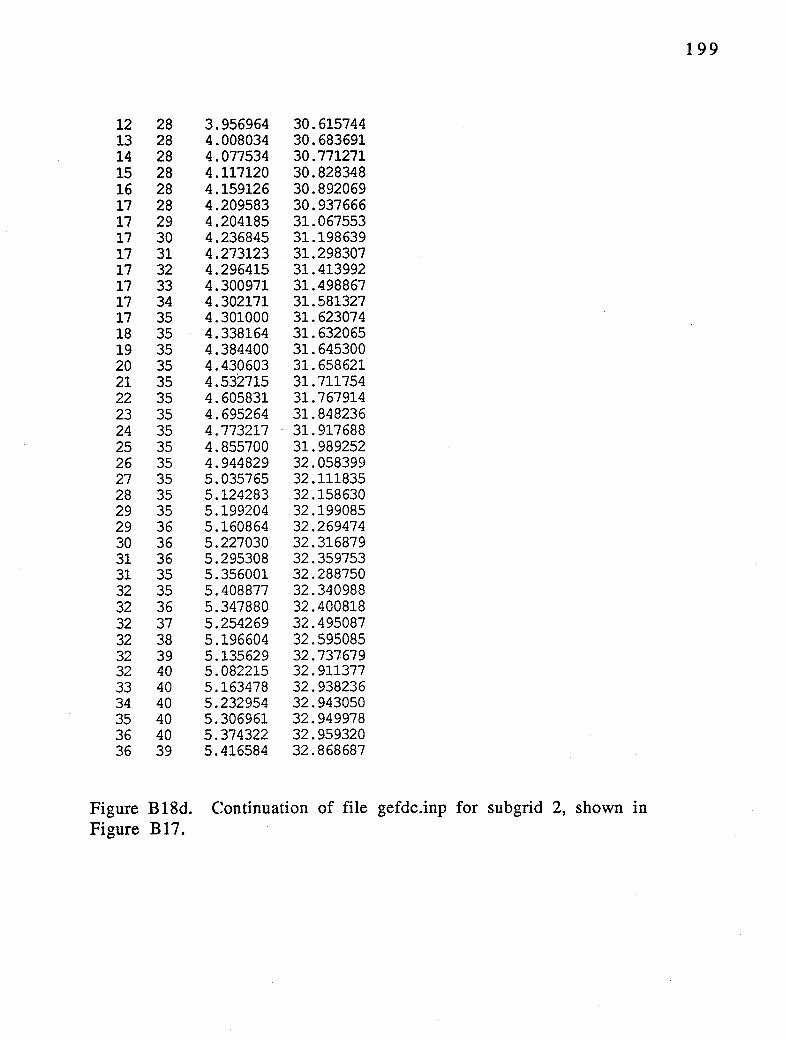
12 28 3.956964 30.615744 13 28 4.008034 30.683691 14 28 4.077534 30.771271 15 28 4.117120 30.828348 16 28 4.159126 30.892069 17 28 4.209583 30.937666 17 29 4.204185 31.067553 17 30 4.236845 31.198639 17 31 4.273123 . 31.298307 17 32 4.296415 31.413992 17 33 4.300971 31.498867 17 34 4.302171 31.581327 17 35 4.301000 31.623074 18 35 4.338164 31.632065 19 35 4.384400 31.645300 20 35 4.430603 31.658621 21 35 4.532715 31.711754 22 35 4.605831 31.767914 23 35 4.695264 31.848236 24 35 4.773217 31.917688 25 35 4.855700 31.989252 26 35 4.944829 32.058399 27 35 5.035765 32.111835 28 35 5.124283 32.158630 29 35 5.199204 32.199085 29 36 5.160864 32.269474 30 36 5.227030 32.316879 31 36 5.295308 32.359753 31 35 5.356001 32.288750 32 35 5.408877 32.340988 32 36 5.347880 32.400818 32 37 5.254269 32.495087 32 38 5.196604 32.595085 32 39 5.135629 32.737679 32 40 5.082215 32. 911377 33 40 5.163478 32.938236 34 40 5.232954 32.943050 35 40 5.306961 32.949978 36 40 5.374322 32.959320 36 39 5.416584 32.868687

Figure B18d. Continuation of file gefdc.inp for subgrid 2, shown in Figure B17.

199

Figure B19. Figure Bl2. NTYPE=5.


200

Cl TITIE Cl (LIMITED TO 80 OiARACTERS)

Indian Ri veir Lagoon, Sub Grid 3 C2 INTEGER INPtrl' C2 NTYPE NBPP IMIN IMAX JMIN JMAX IC JC

5 48 1 54 1 60 54 60 C3 GRAPHICS GRID INFORMATION C3 ISGG IG1 ~IG1 DXCG DYCG NW1'GG

0 50 92 250. 250. 1 C4 CARTESIAN M[) GRAPHICS GRID COORDINATE DATA C4 CDWNl CDU:N2 CDLON3 COLA.Tl CDLA.T2 CDLAT3

1.875 15.0 0.0 17.875 15.0 0.0 CS INTEGER INPUT CS ITRXM ITRHM ITRKM ITRGM NDEPSM


1.8 1.8 1.8 1.E-12 1.E-12 1.E-12 1.E-12 1.E-12 1.E-12 C7 COORDINATE SHIFT PARAMETERS C7 XSHIFT YSHIFT HSCALE RK.JDKI ANGORO

0. Cl. 1000. 1. 5. 0 ca INTERPOLA.TICN SWITCHES ca ISIRKI JSIRKI ISIHIHJ JSIHIHJ

1 0 0 0 C9 NTYPE = 7 SPECIFIED INPUT C9 IB IE JB JE N7RLX NXYIT I'IN7M IJSMD ISMD JSMD RP7 SERRMAX ClO NTYPE = 7 SPECIFIED INPUT ClO X Y IN ORDER (IB, JB) (IE, JB) (IE, JE) (IB, JE) Cll DEPTH INTERPOLA.TION SWITCHES Cll ISIDEP NDEPDAT CDEP RADM ISIDPTYP SURFELV ISVEG NVEGDAT NVEGTYP

0 896 2 .. 5 3 0.167 0 0 0 C12 LAST BCUNDARY POINT INFORMATION Cl2 ILT JLT X(ILT,JLT) Y(ILT,JLT)

41 2 10.771623 20.911531 Cl3 BOUNDARY POJNT INFORMATION Cl3 I J X(I,J) Y(I,J)

40 2 10.680992 20.869270 40 3 10.511944 21.231794 40 4 10.332051 21.688562 40 5 10.185966 22.072828 40 6 10.044719 22.470383 40 7 9.894407 22.863710 40 8 9.746491 23.180916 40 9 9.581670 23.534378 40 10 9.410230 23.973021 40 11 9.254519 24.496237

Figure B20a. File gefdc.inp for subgrid 3, shown in Figure B19.

201

39 11 9.088380 24.473932 39 12 9.040770 24.859980 38 12 8.901817 24.850355 38 13 8.859043 25.249693 38 14 8.798752 25.662931 37 14 8.681543 25.630342 36 14 8.573397 25.601980 36 15 8.490144 25.993475 36 16 8.427410 26.317305 36 17 8.353781 26.569849 36 18 8.205865 26.887056 37 18 8.296495 26.929317 38 18 8.387127 26.971581 39 18 8.500415 27.024408 40 18 8.636361 27.087799 41 18 8. 772307 27.151192 42 18 8.908255 27.214586 43 18 9.021543 27.267414 44 18 9.112172 27.309675 44 17 9.281219 26.947151 44 16 9.412794 26.523020 44 15 9.479142 26 .167774 44 14 9.558780 25.807695 44 13 9.654101 25.366657 44 12 9.746417 24.979389 44 11 9.811546 24.579441 44 10 9.916542 24.164982 44 9 10.098267 23.775270 44 8 10.263088 23.421810 44 7 10.404335 23.024256 44 6 10.508718 22.587444 44 5 10.613714 22.172985 44 4 10.706031 21.785717 44 3 10.874467 21.400841 44 2 11.043514 21.038317 43 2 10.952884 20.996056 42 2 10.862254 20.953794 41 2 10.771623 20.911531

Figure B20b. Continuation of file gefdc.inp for sub grid 3, shown in Figure BI9.

202

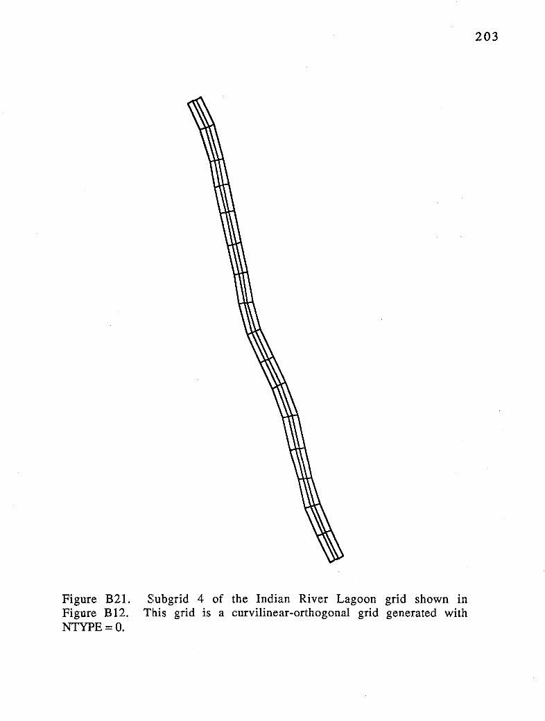
Figure B21. Figure B12. NTYPE=O.


203


Indian River lagoon, Subgrid 4 C2 INTEGER INPUT C2 NTYPE NBPP !MIN IMAX JMIN JMAX IC JC

0 0 1 54 1 60 54 60 C3 GRAPHICS GRID INFORMATION C3 ISGG IG1 JQ.1 DXCG DYCG NWI'GG

0 50 92 250. 250. 1 C4 CARTESIAN AND GRAPHICS GRID COORDINATE DATA C4 CDLONl CDLCN2 CDLON3 CDIATl CDIAT2 CDIAT3

1.875 15.0 0.0 17.875 15.0 0.0 CS INTEGER INPUT CS ITRXM I'J.'RHt.'.l ITRKM ITRQ1 NDEPSM

100 100 100 100 1000 C6 RFAL INPUT C6 RPX RPK RPH RSQXM RSQKM RSQKIM RSQHM RSQHIM RSQHJM

1.8 1.8 1.8 1.E-12 1.E-12 1.E-12 1.E-12 1.E-12 1.E-12 C7 COORDINATE SHIFT PARAMETERS C7 XSHIFT YSHIFT HSCAI.E RKJDKI ANGORO

0. 0. 1000. 1. 7. 0 C8 INI'ERPOIATION SWITCHES C8 !SIRK! JSIRKI ISIHIHJ JSIHIHJ

1 0 0 0 C9 NTYPE = 7 SPECIFIED INPUT C9 IB IE JB JE N7RLX NXYIT ITN7M IJSMD ISMD JSMD RP7 SERRMAX ClO NTYPE = 7 SPECIFIED INPUT ClO X Y IN ORDER (IB, JB) (IE, JB) (IE, JE) (IB, JE) Cll DEPTH INI'ERPOIATION SWITCHES Cll ISIDEP NDEPDAT CDEP RADM ISIDPTYP SURFELV ISVEG NVEGDAT NVEGTYP

0 1054 2 .. 5 3 0.167 0 0 0 Cl2 IAST BOUNDARY POINr INFORMATION Cl2 ILT JLT X(ILT,JLT) Y(ILT,JLT)

1 1 0.0 0.0 Cl3 BOUNDARY POINT INFORMATION Cl3 I J X(I,J) Y(I,J)

Figure B22. File gefdc.inp for subgrid 4, shown m Figure B21, generated with NTYPE = 0.

204

Figure B23. Figure B12. NTYPE=5.


205

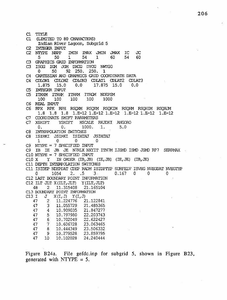
Cl TITIE Cl (LIMITED TO 80 OiARACTERS}

Indian Rive:r Lagoon, Subgrid 5 C2 INTF.Grn INPUT C2 NTYPE NBPP IMIN IMAX JMIN JMAX IC JC

5 50 1 54 1 60 54 60 C3 GRAPHICS GRID INFORMATION C3 ISGG IG1 JQ1 DXCG DYCG NWI'GG

0 50 92 250. 250. 1 C4 CARTESIAN AND GRAPHICS GRID COORDINATE DATA C4 O)LONl O)LCN2 O)L0N3 0)IAT1 0)IAT2 0)1AT3

1.875 15.0 0.0 17.875 15.0 0.0 C5 INTF.Grn INPUT C5 ITRXM ITRHM ITRKM ITRG1 NDEPSM


1.8 1.8 1.8 1.E-12 1.E-12 1.E-12 1.E-12 1.E-12 1.E-12 C7 COORDINATE SHIFT PARAMETERS C7 XSHIFT YSHIFT HSCALE RKJDKI ANGORO

0. 0. 1000. 1. 5.0 ca INI'ERPOIATION SWITCHES ca ISIRKI JSIRKI ISIHIHJ JSIHIHJ

1 0 0 0 C9 NTYPE = 7 SPECIFIED INPUT C9 IB IE JB JE N7RLX NXYIT ITN7M IJSMD ISMD JSMD RP7 SERRMAX Cl O NTYPE = 7 SPECIFIED INPUT ClO X Y IN ORDER (IB, JB) (IE, JB) (IE, JE} (IB, JE} Cll DEPTH INI'ERPOLATION SWITCHES Cll ISIDEP NDEPDAT O)EP RADM ISIDPTYP SURFELV ISVEG NVEGDAT NVEGTYP

0 1054 2 .. 5 3 0.167 0 0 0 Cl2 IAST BOUNDARY POINT INFORMATION Cl2 ILT JLT X(ILT,JLT) Y(ILT,JLT}

48 2 11.315408 21.165104 Cl3 BOUNDARY POINT INFORMATION Cl3 I J X(I,,J) Y(I,J)

47 2 11.224776 21.122841 47 3 11.055729 21.485365 47 4 10.909035 21.847277 47 5 10.797980 22.203743 47 6 10.702049 22.622427 47 7 10.606728 23.063465 47 8 10.444349 23.506332 47 9 10 . .279528 23.859795 47 10 10.102028 24.240444

Figure B24a. File gefdc.inp for subgrid 5, shown m Figure B23, generated with NTYPE = 5.

206

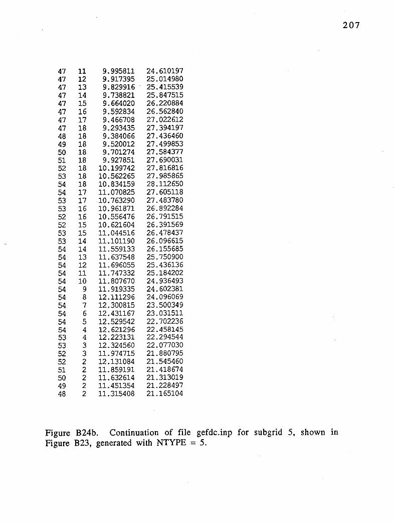
47 11 9.995811 24.610197 47 12 9.917395 25.014980 47 13 9.829916 25.415539 47 14 9.738821 25.847515 47 15 9.664020 26.220884 47 16 9.592834 26.562840 47 17 9.466708 27.022612 47 18 9.293435 27.394197 48 18 9.384066 27.436460 49 18 9.520012 27.499853 50 18 9.701274 27.584377 51 18 9.927851 27.690031 52 18 10.199742 27.816816 53 18 10.562265 27.985865 54 18 10.834159 28.112650 54 17 11.070825 27.605118 53 17 10.763290 27.483780 53 16 10.961871 26.892284 52 16 10.556476 26.791515 52 15 10.621604 26.391569 53 15 11.044516 26.478437 53 14 11.101190 26.096615 54 14 11.559133 26.155685 54 13 11.637548 25.750900 54 12 11.696055 25.436136 54 11 11. 747332 25.184202 54 10 11.807670 24.936493 54 9 11.919335 24.602381 54 8 12.111296 24.096069 54 7 12.300815 23.500349 54 6 12.431167 23.031511 54 5 12.529542 22.702236 54 4 12.621296 22.458145 53 4 12.223131 22.294544 53 3 12.324560 22.077030 52 3 11. 974715 21.880795 52 2 12.131084 21.545460 51 2 11.859191 21.418674 50 2 11.632614 21.313019 49 2 11.451354 21.228497 48 2 11.315408 21.165104

Figure B24b. Continuation of file gefdc.inp for subgrid 5, shown m Figure B23, generated with NTYPE = 5.

207

B.S. SFWMI> Water Conservation Area 2A, Florida

This section describes a curvilinear-orthogonal grid of the South Florida Water Management District's Water Conservation Area 2A southwest of West Palm Beach, Florida. The physical domain grid is shown in Figure~ B25, the cell.inp file in Figure B26, and the gefdc.inp file in Figure B27. The Cartesian graphic grid overlay file, gcell.inp, is shown in Figurn B28, and its equivalent square cell Cartesian grid is shown in Figure B29. The main portion of the curvilinear grid, excluding the lower four cells is based on a quasi-conformal mapping using the NTYPE = 7, option by gefdc.f. The four lower cells were then appended to the grid by hand. The four boundary function subroutines required by the NTYPE = 7, option are shown in Figure B30-B33.

208

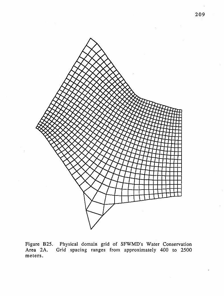
Figure B25. Area 2A. meters.

Physical domain grid of SFWMD's Water Conservation Grid spacing ranges from approximately 400 to 2500

209

C cell.inp file,. i columns and j rows, for w:A2A C 1 2 3 4 C 1234567890123456789012345678901234567890 C

C C

32 31 30 29 28 27 26 25 24 23 22 21 20 19 18 17 16 15 14 13 12 11 10

9 8 7 6 5 4 3 2 1

99999999999999999999999999999999999999 95555555555555555555555555555555555559 99999999999999999999999999999999999999 00000000000009555555555555555555555559 99999999999999999999999999999999999999 95555555555555555555555555555555555559 95555555555555555555555555555555555559 95555555555555555555555555555555555559 95555555555555555555555555555555555559 95555555555555555555555555555555555559 95555555555555555555555555555555555559 95555555555555555555555555555555555559 95555555555555555555555555555555555559 95555555555555555555555555555555555559 95555555555555555555555555555555555559 95555555555555555555555555555555555559 95555555555555555555555555555555555559 95555555555555555555555555555555555559 95555555555555555555555555555555555559 95555555555555555555555555555555555559 95555555555555555555555555555555555559 95555555555555555555555555555555555559 95555555555555555555555555555555555559 95555555555555555555555555555555555559 95555555555555555555555555555555555559 95555555555555555555555555555555555559 95555555555555555555555555555555555559 95555555555555555555555555555555555559 95555555555555555555555555555555555559 99999999999999999999352999999999999999 00000000000000000009939900000000000959 00000000000000000000999000000000000999

1 2 3 4 1234567890123456789012345678901234567890

Figure B26. File cell.inp for WCA2A Grid Shown in Figure B25.

210


SWflM) ~

C2 INTEGER INPUT C2 NTYPE NBPP IMIN IMAX JMIN JMAX IC JC

7 106 1 38 1 28 38 28 C3 GRAPHICS GRID INFORMATION C3 ISGG IG1 JG1 DXCG DYCG NWffiG

1 44 55 600. 600. 1 C4 CARTESIAN AND GRAPHICS GRID COORDINATE DATA C4 CDLONl CDLCN2 CDWN3 CDIATl CDIAT2 CDLAT3

5.1 36.0 0.0 3.9 36.0 0.0 CS INTEGER INPUT CS ITRXM ITRHM ITRKM ITRG1 NDEPSM


1.8 1.8 1.8 l.E-12 1.E-12 1.E-12 1.E-12 1.E-12 1.E-12 C7 COORDINATE SHIFT PARAMETERS C7 XSHIFT YSHIFT HSCALE RK.JDKI ANGORO

0. 0. 1000. 1. 5.04 ca INTERPOIATION SWITOIES ca ISIRKI JSIRKI ISIHIHJ JSIHIHJ

0 0 1 0 C9 NTYPE = 7 SPECIFIED INPUT C9 IB IE JB JE N7RLX NXYIT ITN7M IJSMD ISMD JSMD RP7 SERRMAX

2 38 4 28 1000 1 500 0 0 26 1.0 1.E-8 Cl O NTYPE = 7 SPECIFIED INPUT ClO X Y IN ORDER (IB, JB) (IE, JB) (IE, JE) (IB, JE)

6.76 20.6 31. 9.1 31. 23. 6

15.76 35.6 Cll DEPTH INTERPOIATION SWITOIES Cll ISIDEP NDEPDAT CDEI? RADM ISIDPTYP SURFELV ISVEG NVEGDAT NVEGTYP

1 783 2. .5 2 4.00 1 10710 12 C12 LAST BOONDARY POINT INFORMATION Cl2 ILT JLT X(ILT,JLT) Y(ILT,JLT)

1 1 0.0 0.0 C13 BOUNDARY POINT INFORMATION C13 I J X(I,J) Y(I,J)

Figure B27. File gefdc.inp for WCA2A Grid Shown in Figure B25.

211

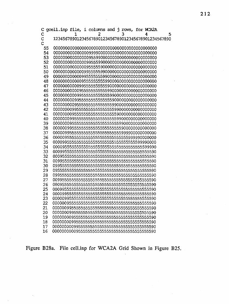
C gcell.inp file, i columns and j rows, for w:A2A C 1 2 3 4 5 C 12345678901234567890123456789012345678901234567890 C

55 00000000000000000000000000000000000000000000 54 00000000000000099990000000000000000000000000 53 00000000000000095599000000000000000000000000 52 00000000000000995559900000000000000000000000 51 00000000000000955555900000000000000000000000 50 00000000000009955555990000000000000000000000 49 00000000000099555555599000000000000000000000 48 00000000000095555555559900000000000000000000 47 00000000000995555555555900000000000000000000 46 00000000000955555555555990000000000000000000 45 00000000009955555555555599000000000000000000 44 00000000099555555555555559000000000000000000 43 00000000095555555555555559900000000000000000 42 00000000995555555555555555990000000000000000 41 00000000955555555555555555590000000000000000 40 00000009955555555555555555599000000000000000 39 00000009555555555555555555559900000000000000 38 00000099555555555555555555555900000000000000 37 00000995555555555555555555555999900000000000 36 00000955555555555555555555555555999990000000 35 00009955555555555555555555555555555599990000 34 00009555555555555555555555555555555555599990 33 00099555555555555555555555555555555555555590 32 00095555555555555555555555555555555555555590 31 00995555555555555555555555555555555555555590 30 09955555555555555555555555555555555555555590 29 09555555555555555555555555555555555555555590 28 09955555555555555555555555555555555555555590 27 00995555555555555555555555555555555555555590 26 00095555555555555555555555555555555555555590 25 00099555555555555555555555555555555555555590 24 00009955555555555555555555555555555555555590 23 00000995555555555555555555555555555555555590 22 00000095555555555555555555555555555555555590 21 00000099555555555555555555555555555555555590 20 00000009955555555555555555555555555555555590 19 00000000955555555555555555555555555555555590 18 00000000995555555555555555555555555555555590 17 00000000099555555555555555555555555555555590 16 00000000009555555555555555555555555555555590

Figure B28a. File cell.inp for WCA2A Grid Shown in Figure B25.

212

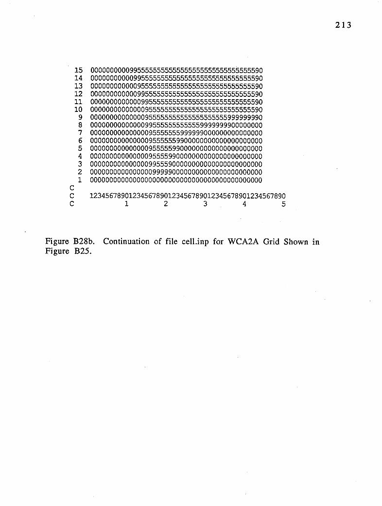
C

15 00000000009955555555555555555555555555555590 14 00000000000995555555555555555555555555555590 13 00000000000095555555555555555555555555555590 12 00000000000099555555555555555555555555555590 11 00000000000009955555555555555555555555555590 10 00000000000000955555555555555555555555555590

9 00000000000000955555555555555555555999999990 8 00000000000000995555555555559999999900000000 7 00000000000000095555555999999000000000000000 6 00000000000000095555559900000000000000000000 5 00000000000000095555599000000000000000000000 4 00000000000000095555990000000000000000000000 3 00000000000000099555900000000000000000000000 2 00000000000000009999900000000000000000000000 1 00000000000000000000000000000000000000000000

C 12345678901234567890123456789012345678901234567890 C 1 2 3 4 5

Figure B28b. Continuation of file cell.inp for WCA2A Grid Shown in Figure B25.

213

--

I

Figure B29. Square cell Cartesian grid representing same region as shown in Figure B 25. This grid corresponds to the file gcell.inp m Figure B28.

214

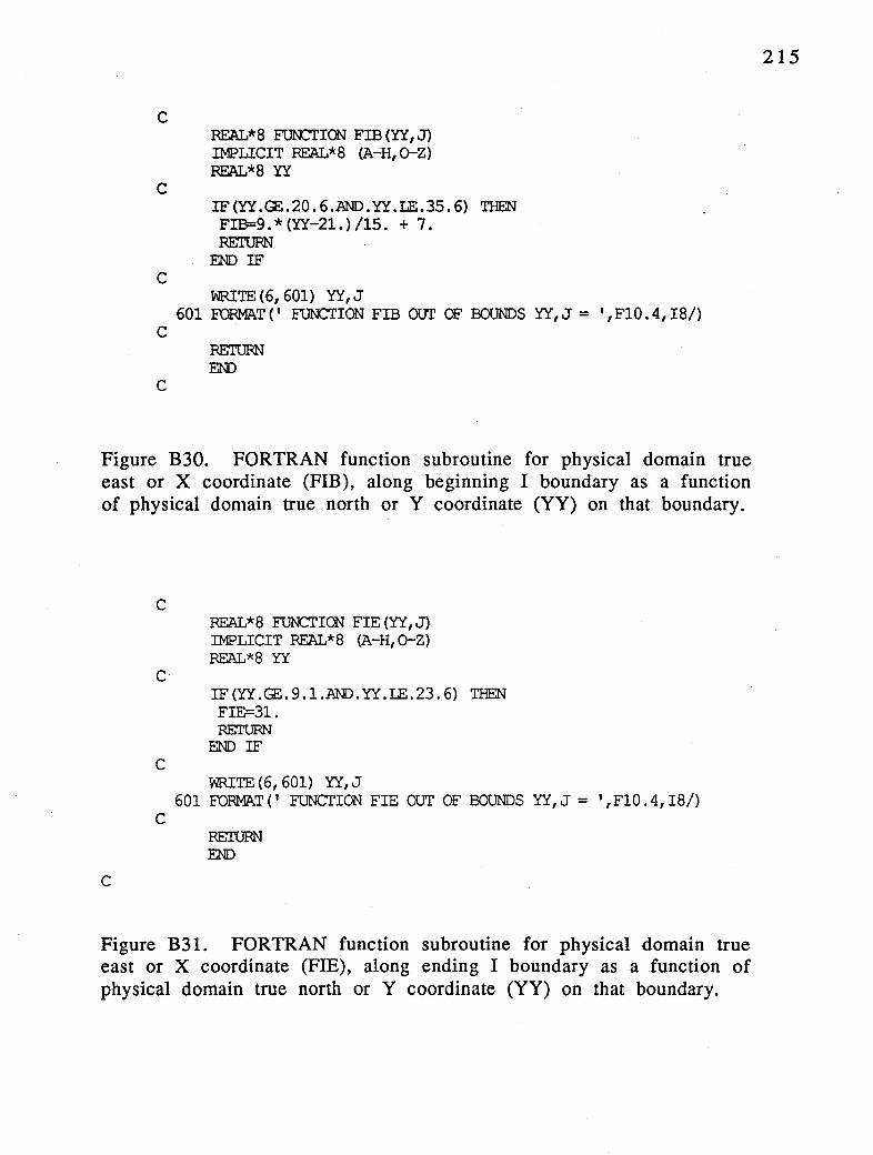
C

C

C

REAL*8 FUNCTION FIB (YY, J) IMPLICIT REAL*8 (A-H, 0-Z) REAL*8 YY

IF(YY.GE:.20.6.AND.YY.LE.35.6) THEN FIB=9.*(YY-21.)/15. + 7. RETURN

END IF

WRITE(6,601) YY,J 601 FORMAT(' FUNCTION FIB OUT OF BOUNDS YY,J = ',F10.4,I8/)

C

C

RETURN END

Figure B30. FORTRAN function subroutine for physical domain true east or X coordinate (FIB), along beginning I boundary as a function of physical domain true north or Y coordinate (YY) on that boundary.

C

C

C

C

REAL*8 FUNCTION FIE(YY,J) IMPLICIT REAL*8 (A-H,0-Z) REAL*8 YY

IF(YY.GE:.9.1.AND.YY.LE.23.6) THEN FIE=31. RETURN

END IF

WRITE(6,601) YY,J 601 FORMAT (' FUNCTION FIE OUT OF BOUNDS YY, J = ',FlO. 4, I8/)

C RETURN END

Figure B31. FORTRAN function subroutine for physical domain true east or X coordinate (FIE), along ending I boundary as a function of physical domain true north or Y coordinate (YY) on that boundary.

215

C

C

C

C

REAL*8 FUNCTICN GJB (XX, I) IMPLICIT REAL*8 (A-H,0-Z) REAL*8 XX

IF(XX.GE.6.76.AND.XX.LT.8.76) THEN X=XX-6.76 GJB=20.6-0.6*X-(2.254-0.203*X)*X*X/7.7 RETURN

END IF

IF(XX.GE.8.76.AND.XX.LT.14.7) THEN GJB=-11.2*(XX-7.)/7.7 + 21. RETURN

END IF

IF(XX.GE.14.7.AND.XX.LT.19.4) THEN C GJB=-2.l*(XX-14.7)/4.7 + 9.8

X=XX-14.7 CIMP=6.764968/(4.7*4.7) D'IMP=-2.028605/(4.7*4.7*4.7) GJB=9.8-11.2*X/7.7+(C'IMP+DTMP*X)*X*X RETURN

END IF C

C

IF(XX.GE.19.4.AND.XX.LE.29.0) THEN GJB=l.S*(XX-19.4)/11.6 + 7.7 RETURN

END IF

IF (XX.GE.29.0 .AND.XX.LE.31.) THEN X=XX-31. . GJB=9.1-(0.63+0.085*X)*X*X/11.6 RETURN

END IF C

WRI'IE(6,601) XX,I 601 FOFMAT(' FUNCTION GJB CUT OF BOUNDS XX,I = ',F10.4,I8/)

C

C

RETURN END

Figure B32. FORTRAN function subroutine for physical domain true north or Y coordinate (GJB), along beginning J boundary as a function of physical domain true east or X coordinate (XX) on that boundary.

216

C

C

C

C

C

C

C

REAL*8 FUN:TION GJE (XX, I) IMPLICIT REAL*8 (A-H,0-Z) REAL*8 XX

IF(XX.GE.15.76.AND.XX.LT.17.76) THEN X=XX-15. 76 GJE=35.6-0.6*X-(l.696-0.082*X)*X*X/7.5 RETURN

END IF

IF(XX.GB.17.76.AND.XX.LT.22.5) THEN GJE=-10.3*(XX-16.)/7.5 + 36. RETURN

END IF

IF(XX.GB.22.5.AND.XX.LT.24.5) THEN X=XX-22.5 GJE=(203.05-10.3*X+2.*X*X)/7.5 RETURN

END IF

IF(XX.GB.24.5.AND.XX.LT.29.0) THEN GJE=-2.3*(XX-23.5)/7.5 + 25.7 RETURN

END IF

IF(XX.GB.29.0.AND.XX.IB.31.0) THEN X=XX-31. GJE=23.6+(1.175+0.2*X)*X*X/7.5 RETURN

END IF

WRITE(6,601) XX,I 601 FORMAT (' FUNCTION GJE OUT OF BOUNDS xx, I = ', FlO. 4, I8/)

C C

C

RETURN END

Figure B33. FORTRAN function subroutine for physical domain true north or Y coordinate (GJE), along ending J boundary as a function of physical domain true east or X coordinate (XX) on that boundary.

217

B.6. Chesapeake Bay

This section describes a square cell Cartesian grid of the Chesapeake Bay. The physical domain grid is shown in Figure B34, the cell.inp file, Figure B35, and the gefdc.inp file, Figure B36. The grid was generated with the NTYPE = 9, option by gefdc.f.

218

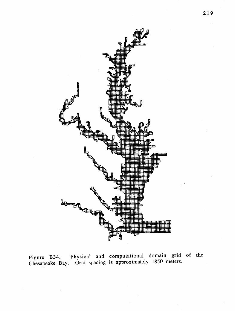
219

Figure B34. Physical and computational domain grid of the Chesapeake Bay. Grid spacing is approximately 1850 meters.

C cell.irp file, i across arrl j q,, for ches bay CO 1 2 3 4 5 6 7 8 9 C 123456789012345678901234567890123456789012345678901234567890123456789012345678901234567890123456 C 180 000000000000000000000000000000000000000000000000000000000000000000000000000000000000000000000000 179 000000000000000000000000000000000000000000000000000000000000000000000000000000000000000000000000 178 000000000000000000000000000000000000000000000000000000000000000000000000000000000000000000000000 177 000000000000000000000000000000000000000000000000000000000000000000000000000000000000000000000000 176 000000000000000000000000000000000000000000000000000000000000000000000000000000000000000000000000 175 000000000000000000000000000000000000000000000000000000000000000000000000000000000000000000000000 174 000000000000000000000000000000000000000000000000000000000000000000000000999000000000000000000000 173 000000000000000000000000000000000000000000000000000000000000000000099909959099900000000000000000 172 000000000000000000000000000000000000000000000000000000000000000000995999559095900000000000000000 171 000000000000000000000000000000000000000000000000000000000000000000945551529095900000000000000000 170 000000000000000000000000000000000000000000000000000000000000000009955555599995900000000000000000 169 000000000000000000000000000000000000000000000000000000000000000009455555599452900000000000000000 168 000000000000000000000000000000000000000000000000000000000000000009555555994599900000000000000000 167 000000000000000000000000000000000000000000000000000000000009990009993555942359000000000000000000 166 000000000000000000000000000000000000000000000000000000000009590000999552429999000000000000000000 165 000000000000000000000000000000000000000000000000000000000009590009954555599000000000000000000000 164 000000000000000000000000000000000000000000000000000000000099590099455555990000000000000000000000 163 000000000000000000000000000000000000000000000000000009999994290994555552900000000000000000000000 162 000000000000000000000000000000000000000000000000000009551995999955555599999990000000000000000000 161 000000000000000000000000000000000000000000000000000009935995994555555555555590000000000000000000 160 000000000000000000000000000000000000000000000000000000995995145555299999999990000000000000000000 159 000000000000000000000000000000000000000000000000000000095593555555990000000000000000000000000000 158 000000000000000000000000000000000000000000000000000009995595555299900000000000000000000000000000 157 000000000000000000000000000000000000000000000000000099545545555190000000000000000000000000000000 156 000000000000000000000000000000000000000000000000000995555555555290000000000000000000000000000000 155 000000000000000000000000000000000000000009999990000995555555552990000000000000000000000000000000 154 000000000000000000000000000000000000000009555199009945555555529900000000000000000000000000000000 153 000000000000000000000000000000000000000009993519909555555555599000000000000000000000000000000000 152 000000000000000000000000000000000000000000094555999945555555290000000000000000000000000000000000 151 000000000000000000000000000000000000000000099935199455555555990000000000000000000000000000000000 150 000000000000000000000000000000000000000000000995555555555552900000000000000000000000000000000000 149 000000000000000000000000000000000000000000000095555555555559900000000000000000000000000000000000 148 000000000000000000000000000000000000000000000099935555555559900000000000000000000000000000000000 147 000000000000000000000000000000000000000000000000993555555551900000000000000000000000000000000000 146 000000000000000000000000000000000000000000000000099555555555999999990000000000000000000000000000 145 000000000000000000000000000000000000000000000000009355555555199545590000000000000000000000000000 144 000000000000000000000000000000000000000000000099999955555555595559990000000000000000000000000000 143 000000000000000000000000000000000000000000000095555455555555595529000000000000000000000000000000 142 000000000000000000000000000000000000000000000099935555555555595299000000000000000000000000000000 141 000000000000000000000000000000000000000000000999999955555555295190000000000000000000000000000000 140 000000000000000000000000000000000000000000000951990995552355195590000000000000000000000000000000 139 000000000000000000000000000000000000000000000995199945559955555590000000000000000000000000000000 138 oooooooooooooooooooooooooooooooooooooooooccooo99593155559935555290000000000000000000000000000000 131 ooooooooooooooooooooooooooooooooooooooooooccooo9355555529999352990000000000000000000000000000000 136 00000000000000000000000000000000000000000Cc'00999935555599999999900000000000000000000000000000000 135 000000000000000000000000000000000000000000000959995555599945559000000000000000000000000000000000 134 000000000000000000000000000000000000000000000955195555595955559000000000000000000000000000000000 133 000000000000000000000000000000000000000000000993555555295155559000000000000000000000000000000000 132 000000000000000000000999000000000000000000000099555555995555559000000000000000000000000000000000 131 000000000000000000000959000000000000000000000994555555995555559990000000000000000000000000000000 130 000000000000000000000959000000000000000000000955555555945552555590000000000000000000000000000000 129 000000000000000000000959000000000000000000000999555555455529555990000000000000000000000000000000 128 000000000000000000000959000000000000000000000099555555555299555900000000000000000000000000000000 127 000000000000000000000959000000000000000000000094555555555999935990000000000000000000000000000000 126 000000000000000000000959000000000000000000009995555555555900995190000000000000000000000000000000 125 000000000000000000000959000000000000000000009455555555559999995590000000000000000000000000000000 124 000000000000000000000959000000000000000000009555555555559599599990000000000000000000000000000000 123 000000000000000000000959000000000000000000009355555555559595559000000000000000000000000000000000

Figure B35a. File cell.inp for Chesapeake Bay Grid Shown in Figure B34.

220

122 000000000000000000999959000000000000000000009935555555524595599999900000000000000000000000000000 121 000000000000000009945559000000000000000000000995555555595555599455900000000000000000000000000000 120 000000000000000099552999000000000000000000000095555555593555519599900000000000000000000000000000 119 00000000000099909459990°0000000000000000000000095555555555555555599000000000000000000000000000000 118 000000000000959095590000000000000000000000000095555555555555555559000009990000000000000000000000 117 000000000009959993590000000000000000000000000095555555555555555559999009590000000000000000000000 116 000000000009559455290000000000000000000000000095555555555535355955159909590000000000000000000000 115 000000000009555552990000000000000000000000000095555555555519939955551999590000000000000000000000 114 000000000099555999900000000000000000000000000095555555555559999993555194590000000000000000000000 113 000000000095552900000000000000000000000999000095555555555299999099993552990000000000000000000000 112 000000000995555900000000000000000000000959000095555555555519959000099999900000000000000000000000 111 000000000945599900000000000000000000000959000095555555555551459000000000000000000000000000000000 110 000000009955990000000000000000000000000959000095555555555555559000000000000000000000000000000000 109 000000009452900000000000000000000000000959000093555555555552999000000000000000000000000000000000 108 000000099559900000000999000000000000000959000099555555559959900000000000000000000000000000000000 107 000000094559000000000959000000000000000959990009355555559999000000000000000000000000000000000000 106 000000095559000009999959900000000000000955190009935555551990000000000000000000000000000000000000 105 000000095559000009599451900000000000000995599900993555555190000000000000000000000000000000000000 104 000000093559900009594555900000000000000099551999099355555590000000000000000000000000000000000000 103 000000099551900099545555990000000000000009935559909955555599000000000000000009990000000000000000 102 000000095555999994555235190099999000000000993551990995555519999000000000000009590000000000000000 101 000000099355199455552995590095519000000000099935190095555551959990000099999009590000000000000000 100 000000009955555559999995599099959000000000000999590995555555155190000094519999590000000000000000

99 000000000935555299000095519909459000000000000009599945555555535590000995559945590000000000000000 98 000000000999999990000995555999359900000000000009555155555555545999000945529955990000000000000000 97 000000000000000000000955555599951900000000000009935555555555535559990955999459900000000000000000 96 000000000000000000000993555519935900000000000000999994555555551959599935999559000000000000000000 95 00000000000000000000009955555199599099999900000000009555555555595455999519954 9000000000000000000 94 000000000000000000000009935555555199955559000000000095555555555135529945519519999000000000000000 93 000000000000000000000000995555555519425999990000000095555555555519551955529559459900000000000000 92 000000000000000000000000955555555551555555199000000093555555555555555135555555555900000000000000 91 000000000000000000000000993555555555555555559990099999555555555555555555555555299900000000000000 90 000000000000000000000000099935555555555555555190095909355555555555552935555529990000000000000000 89 000000000000000000000000000993555555555555555590095909935555555555559995559999000000000000000000 88 000000000000000000000000000099999995559555555599995900995555555555551995559999999990000000000000 87 000000000000000000000000000000000099559931955551995900993555555555555555559945955590000000000000 86 000000000000000000000000000000000009959999955555555999955555555555555524551455559990000000000000 85 000000000000000000000000000000000000999000935555555159935555555555555595555555529000000000000000 84 000000000000000000000000000000000000000000993555555551995555555555555593555555299000000000000000 83 000000000000000000000000000000000000000000099955555555995555555555555555555555999999000000000000 82 000000000000000000000000000999000000000000000935555555193555555555555555555555555559000000000000 81 000000000000000000000000000959000000000000000955555555555555555555555555555555559999000000000000 80 000000000000000000000000000959000000000000000923555555555555555555555593555555999000000000000000 79 000000000000000000000000000959000000000000000999935555555555555555555559955555900000000000000000 78 000000000000000000000000000959990000000000000000955555555555555555555599455552900000000000000000 77 OOOOOOOOOOOOOC0000000000000955590000000000000000939355555555555555555599555559909999999999999000 76 000000000000000000000000000999599000000000000000999993555555555555555599555555999455555555559000 75 000000000000000000000000000009319990000000000000000099993555555555555514555559994555555555559000 74 000000000000000000000000000009955199000000000000000000099355555555555555555559945555599999999000 73 000000000000000000000000000000993519000000000000000000009993555555555555555555555555999900000000 72 000000000000000000000000000000099959900000000000000000000099555555555555555555555555555900000000 71 000000000000000000000000000000000955990000000000000000000009555555555555555555555555555900000000 70 000000000000000000000000000000000995199000000000000000000009555555555555555555555555555900000000 69 000000000000000000000000000000000093519900000000000000009999555555555555955555555555559900000000 68 000000000000000000000000000000000099551999000000000000009594555555555555955555555555529000000000 67 000000000000000000000000000000000009355519900000000000009555555555555555555555555555599000000000 66 "000000000000000000000000000000000009935555999000000000009555555555555555555555555995590000000000 65 000000000000000000000000000000000000999555519900000000009555555555555555555555555599990000000000 64 000000000000000000000000000000000000009355551900000000009555555555555555555555555590000000000000 63 000000000000000000000000000000000000009999555900000000009555555555555555555555552990000000000000 62 000000000000000000000000000000000000000009955990999000009555555555555555555555555900000000000000 61 000000000000000000000000000000000000000000955590959000009355555555555555555555559900000000000000

Figure B35b. Continuation of file cell.inp for Chesapeake Bay Grid Shown in Figure B34.

221

60 000000000000000000000000000000000000000000935590959000099455555555555555555555599000000000000000 59 0000000000000000000000()0000000000000000000995599959000095555555555555555555555590000000000000000 58 0000000000000000000000()0000000000000000000095519559990095555555555555555555555990000000000000000 57 0000000000000000000000()0000000000000000000093555555199995355555555555555555559900000000000000000 56 0000000000000000000000()0000000000000000000099355555551999935555555555555555555900000000000000000 55 0000000000000000000000()0000000000000000000009999999555555555555555555555555595900000000000000000 54 0000000000000000000()00()0000000000000000000000000009555555555555555555555555599900000000000000000 53 0000000000000000000()00()0000000000000000000000000009993555555555555555555555990000000000000000000 52 000000000000000000000000000000000000000000000000000099999955555555555555555900000000000000000000 51 0000000000000000000000()0000000000999000000000000009999945555555555555555555900000000000000000000 SO 0000000000000000000()00()0000000009959900000000000009555555555555555555555552900000000000000000000 49 0000000000000000000000()0000000009551990000000000009999955535555555555555559900000000000000000000 48 0000000000000000000000()0000000009935190000000000000000995595555555555555559000000000000000000000 47 0000000000000000000000()0000000000993599000000000000000099955555555555555559000000000000000000000 46 0000000000000000000000()0000000000099519900000000000000000995555555555555529000000000000000000000 45 0000000000000000000000()0000000000009351900000000000000000099555555555555599000000000000000000000 44 0000000000000000000000()0000000000009935990000000000999999009555555555555599000000000000000000000 43 0000000000000000000()0000000000000000993599000000000959959009555555555555559000000000000000000000 42 000000000000000000000000000000000000099559900000099959959009555555555555559000000000000000000000 41 000000000999000000000000000000000000009351990000095555159099555555555555599000000000000000000000 40 000000000959000000000000000000000000009935199000099555559995555555555555290000000000000000000000 39 000000000959999900000000000000000000000995519000009955555995555555555552990000000000000000000000 38 000000000951451999999999990000000000000093559900099955555195555555555559900000000000000000000000 37 000000000955555555555945190000000000000099555990095525555555555555555559990000000000000000000000 36 000000000999932999995429590000000000000009935599999993555555555555555555590000000000000000000000 35 000000000000999900095599599000000000000000993551909999555555555555555559990000000000000000000000 34 000000000000000000099999319999990000000000099355999455555555555555555559000000000000000000000000 33 000000000000000000000009951945199990000000009935555555555555555555555559000000000000000000000000 32 000000000000000000000000993555555599999999900999355555555555555555555559000000000000000000000000 31 000000000000000000000000099935555519355551900009999935555555555555555559900000000000000000000000 30 000000000000000000000000000999999355555355990000000995555555555555555555990000000000000000000000 29 000000000000000000000000000000009935552955190000000955555555555555555555190000000000000000000000 28 000000000000000000000000000000000999559955590000000955995555555555555555590000000000000000000000 27 000000000000000000000000000000000009999955990000000999993555555555555555599000000000000000000000 26 000000000000000000000000000000000000000955999000000000099355555555555555519000000000000000000000 25 000000000000000000000000000000000000000955519900000000994555555555555555599000000000000000000000 24 000000000000000000000000000000000000000955551999000000955295555555555555599999999999999999999999 23 000000000000000000000000000000000000000955555559000000999945555555555555555555555555555555555559 22 000000000000000000000000000000000000000955555559990000000955555555555555555555555555555555555559 21 000000000000000000000000000000000000000935555555199000000955555555555555555555555555555555555559 20 000000000000000000000000000000000000000999995555519000999955555555555555555555555555555555555559 19 000000000000000000000000000000000000000000095555559999945455555555555555555555555555555555555559 18 000000000000000000000000000000000000000000099955551994555555555555555555555555555555555555555559 17 000000000000000000000000000000000000000000000995555945555555555555555555555555555555555555555559 16 000000000000000000000000000000000000000000000099355555553519555555555555555555555555555555555559 15 000000000000000000000000000000000000000000000009455555559999935555555555555555555555555555555559 14 000000000000000000000000000000000000000000000009555552359900999935555529999999999999999999999999 13 000000000000000000000000000000000000000000000009955559951900000999959999000000000000000000000000 12 000000000000000000000000000000000000000000000099559999935900000000999000000000000000000000000000 11 000000000000000000000000000000000000000000000095299000955900000000000000000000000000000000000000 10 000000000000000000000000000000000000000000000095990000935900000000000000000000000000000000000000 9 000000000000000000000000000000000000000000000095900000999900000000000000000000000000000000000000 8 000000000000000000000000000000000000000000000099900000000000000000000000000000000000000000000000 7 000000000000000000000000000000000000000000000000000000000000000000000000000000000000000000000000 6 000000000000000000000000000000000000000000000000000000000000000000000000000000000000000000000000 5 000000000000000000000000000000000000000000000000000000000000000000000000000000000000000000000000 4 000000000000000000000000000000000000000000000000000000000000000000000000000000000000000000000000 3 000000000000000000000000000000000000000000000000000000000000000000000000000000000000000000000000 2 000000000000000000000000000000000000000000000000000000000000000000000000000000000000000000000000 1 000000000000000000000000000000000000000000000000000000000000000000000000000000000000000000000000

Figure B35c. Continuation of file cell.inp for Chesapeake Bay Grid Shown in Figure B34.

222

Cl TITIE Cl (LIMITED TO 80 OIARACTERS)

chesapeake bay cartesian, 11 input, utm output C2 INTEGER INPUT C2 NTYPE NBPP !MIN IMAX JMIN JMAX IC JC

9 0 1 97 1 181 96 180 C3 GRAPHICS GRID INFORMATION C3 ISGG IG1 JG1 DXCG DYCG nwtgg

1 96 180 1850. 1850. 1 C4 CARTESIAN AND GRAPHICS GRID CCX>RDINATE DATA C4 (l)I.DNl (l)r.m2 (l)L0N3 (l)IATl (l)IAT2 (l)IAT3

-77.5 1.25 -0.625 36.7 1.0 -0.5 C5 INTEGER INPUT C5 ITRXM ITRHM ITRKM ITRGM


1.8 1.8 1.8 1.E-12 1.E-12 1.E-12 1.E-12 l.E-12 1.E-12 C7 COORDINATE SHIFT PARAMETERS C7 XSHIFT YSHIFT HSCALE RKJDKI ANGORO

0. 0. 1000. 1. 7.0 C8 INTERPOIATION SWI'IOIBS ca ISIRKI JSIRKI ISIHIHJ JSIHIHJ

1 0 0 0 C9 NTYPE = 7 SPECIFIED INPUT C9 IB IE JB JE NINI'IM N7REIAX I'IN7MAX SERB.MAX ClO NTYPE = 7 SPECIFIED INPUT ClO X Y IN ORDER (IB, JB) (IE, JB) (IE, JE) (IB, JE) Cll DEPTH INTERPOIATION SWITQIBS Cll ISIDEP NDEPDAT (l)EP RADM isidptyp surfelv

0 79431 2. 1. 1 0. 0 0 0 Cl2 LAST BCXJNDARY POINT INFORMATION Cl2 ILT JLT X{ILT,JLT) Y(ILT,JLT)

1 1 1 1 Cl3 BOUNDARY POINT INFORMATION Cl3 I J X{I,J) Y{I,J)

Figure B36. File gefdc.inp for Chesapeake Bay Grid Shown in Figure B34.

223

user's manual for the environmental fluid dynamics

Documents