user logs for query disambiguation - findwise
TRANSCRIPT

User Logs for QueryDisambiguation
Casper Andersen and Daniel ChristensenSupervised by: Christina Lioma
Submitted in total fulfillment of the requirementsof the degree of Master of Science
June 17, 2013
Department of Computer ScienceUniversity of Copenhagen

Abstract
The purpose of an information retrieval (IR) system is to obtain the mostrelevant information from a data source given a user query. One of themajor issues within IR is query disambiguation, which deals with mainlyambiguous or otherwise vague queries lacking sufficient information for theIR system to provide satisfactory results. E.g. a user query such as bark
could refer to the sound a dog makes, the skin of a tree or a three-mastedsailing ship. Query disambiguation in this case should aim at making aqualified guess of the user’s intention, for instance by analyzing the user’sbehavior or logged activities.
This thesis deals with the problem of query disambiguation by usinglogged user activities (user search logs). The underlying motivation is thatuser search logs may contain valuable information about user behavior suchas which documents were clicked from the returned results in response toa query, or the retrieval rank of the clicked document. Such ’query-loggedactivities’ can be used to disambiguate potentially vague queries [37]. Thestate of the art approach of Wang & Zhai [37] reformulates queries bysubstituting or adding query terms on the basis of evidence extracted fromqueries from the user search logs.
Departing from the approach of Wang & Zhai, we present a query refor-mulation approach that substitutes or adds a term to a query on the basis ofevidence extracted, not from logged queries, but from clicked documents.By clicked documents we mean those documents that a user has chosento view among the results retrieved from a search engine given a query.Unlike queries, which are very short and consist of mainly keyword-basedtext, clicked documents are long and contain a combination of keywordsbut also other words, such as function words. Our method aims to selectthe most salient parts of the clicked documents with respect to a query anduses these for query reformulation.
A thorough experimental evaluation of our approach, using both binaryand graded relevance assessments, on data provided by the search engine ofa large provider of legal content (Karnov Group) reveals that our approachperforms comparably to the state of the art.

Acknowledgements
We would like to thank Findwise, and especially our on-site supervisorsShen Xiaodong and Paula Petcu, who have provided us with office space,support, feedback and contact to Karnov Group. Rasmus Hentze and DennisPeitersen receive our thanks for being our contacts at Karnov Group andfor providing search logs, access to their search engine and feedback on thethesis.
A special thanks to Christina Lioma for her supervision and commit-ment in this thesis. The help and guidance provided was indispensable incompletion of this thesis.

List of Tables
2.1 Example of how the average rank of a document could mapto a relevance score. . . . . . . . . . . . . . . . . . . . . . . 8
2.2 An example on computing MAP@5 for two different queries. 12
3.1 Example of the terms insurance, damage and auto addedfor all possible positions to the query car wash. . . . . . . . 32
4.1 The number of unique terms and salient terms in the datasetof Wang & Zhai and ACDC. . . . . . . . . . . . . . . . . . 43
4.2 The avg. occurrence of unique terms in the dataset of Wang& Zhai and ACDC. . . . . . . . . . . . . . . . . . . . . . . 44
5.1 Overview of the three experiments we design and perform inthis chapter. . . . . . . . . . . . . . . . . . . . . . . . . . . 46
5.2 Overview of the early and full dataset. . . . . . . . . . . . . 485.3 The terms left between the different steps of filtering of the
queries on the early dataset. . . . . . . . . . . . . . . . . . 525.4 Analysis of the number of suggestions for term substitution
for τ = 0.001. . . . . . . . . . . . . . . . . . . . . . . . . . 575.5 Analysis of the number of suggestions for term addition with
τ values 0.001 and 0.0005. . . . . . . . . . . . . . . . . . . 575.6 Analysis of the number of suggestions for term addition on
the candidates for the sampled set. . . . . . . . . . . . . . . 615.7 How we chose the best query reformulation suggestion. In
this example suggestion 4 is the best. . . . . . . . . . . . . 685.8 Term substitution overall performance for easy, medium and
hard queries on the early dataset for Wang & Zhai’s approach. 735.9 Term substitution overall performance for easy, medium and
hard queries on the full dataset for Wang & Zhai’s approach. 745.10 Term addition overall performance for easy, medium and
hard queries on the early dataset for Wang & Zhai’s approach. 745.11 Term addition overall performance for easy, medium and
hard queries on the full dataset for Wang & Zhai’s approach. 755.12 Distribution of the difficulty of queries on the early and full
dataset. . . . . . . . . . . . . . . . . . . . . . . . . . . . . 755.13 Distribution of user votes between the original query and the
reformulated query by the Wang & Zhai approach. . . . . . 76
iii

5.14 User evaluation results divided up in one and two-wordedoriginal queries for Wang & Zhai’s term sustitution. . . . . . 76
5.15 User evaluation results divided up in one and two-wordedoriginal queries for Wang & Zhai’s term addition. . . . . . . 76
5.16 The evaluation metric scores of the user evaluated queriesgenerated by the Wang & Zhai’s approach. . . . . . . . . . 77
5.17 Top-10 most improved query reformulations by Wang &Zhai’s term substitution measured by MAP . . . . . . . . . 78
5.18 Top-10 most hurt query reformulations by Wang & Zhai’sterm substitution measured by MAP . . . . . . . . . . . . . 78
5.19 Top-10 most improved query reformulations by Wang &Zhai’s term addition measured by MAP . . . . . . . . . . . 79
5.20 Top-10 most hurt query reformulations by Wang & Zhai’sterm addition measured by MAP . . . . . . . . . . . . . . . 79
5.21 Top substitution replacements and top added terms amongthe top-5 query formulation suggestions generated by W&Z. 80
5.22 Term substitution run on the full dataset for ACDC, for µ =500 and τ = 0.005. . . . . . . . . . . . . . . . . . . . . . . 82
5.23 Term addition run on the full dataset for ACDC, for µ = 500and τ = 0.0005. . . . . . . . . . . . . . . . . . . . . . . . . 82
5.24 Distribution of user votes between the original query and thereformulated query by the ACDC approach. . . . . . . . . . 83
5.25 User evaluation results divided up in one and two-wordedoriginal queries for ADCD’s term sustitution. . . . . . . . . . 84
5.26 User evaluation results divided up in one and two-wordedoriginal queries for ACDC’s term addition. . . . . . . . . . . 84
5.27 The evaluation metric scores of the user evaluated queriesgenerated by the ACDC approach. . . . . . . . . . . . . . . 84
5.28 Top-10 most improved query reformulations by ACDC’s termsubstitution measured by MAP . . . . . . . . . . . . . . . . 85
5.29 Top-10 most hurt query reformulations by ACDC’s term sub-stitution measured by MAP . . . . . . . . . . . . . . . . . . 86
5.30 Top-10 most improved query reformulations ACDC’s by termaddition measured by MAP . . . . . . . . . . . . . . . . . . 86
5.31 Top-10 most hurt query reformulations by ACDC’s term ad-dition measured by MAP . . . . . . . . . . . . . . . . . . . 87
5.32 Top substitution replacements and top added terms amongthe top-5 query formulation suggestions generated by ACDC. 88
5.33 Term substitution overall performance for hard queries onthe full dataset for the merged model for µ = 3,000 andτ = 0.05. . . . . . . . . . . . . . . . . . . . . . . . . . . . . 89
5.34 Term addition overall performance for hard queries on thefull dataset for the merged model for µ = 3,000 and τ = 0.0005. 90
5.35 Distribution of user votes between the original query and therefor- mulated query by the merged approach. . . . . . . . . 90
5.36 User evaluation results divided up in one and two-wordedoriginal queries for the merged approach for term substitution. 91
5.37 User evaluation results divided up in one and two-wordedoriginal queries for the merged approach for term addition. . 91

5.38 The evaluation metric scores of the user evaluated queriesgenerated by the merged approach . . . . . . . . . . . . . . 91
5.39 Top-10 most improved query reformulations by term substi-tution measured by MAP generated by the merged approach. 92
5.40 Top-10 most hurt query reformulations by term substitutionmeasured by MAP generated by the merged approach. . . . 93
5.41 Top-10 most improved query reformulations by term additionmeasured by MAP generated by the merged approach. . . . 93
5.42 Top-10 most hurt query reformulations by term additionmeasured by MAP generated by the merged approach. . . . 94
5.43 Top substitution replacements and top added terms amongthe top-5 query formulation suggestions generated by themerged approach. . . . . . . . . . . . . . . . . . . . . . . . 95
B.1 Term substitution run on different metrics for different valuesof µ. These numbers are used only for determination of µ
and based on a small set of data (see section 5.2). . . . . . 112B.2 Term addition, threshold = 0.001 run on different metrics
for different values of µ. These numbers are used only fordetermination of µ and based on a small set of data (seesection 5.2). . . . . . . . . . . . . . . . . . . . . . . . . . . 113
B.3 Term addition, threshold = 0.0005 run on different metricsfor different values of µ. These numbers are used only fordetermination of µ and based on a small set of data (seesection 5.2). . . . . . . . . . . . . . . . . . . . . . . . . . . 114
B.4 Term substitution run on different metrics for different valuesof µ, for t = 0.005. . . . . . . . . . . . . . . . . . . . . . . 115
B.5 Term substitution run on different metrics for different valuesof µ, for t = 0.002. . . . . . . . . . . . . . . . . . . . . . . 116
B.6 Term substitution run on different metrics for different valuesof µ, for t = 0.001. . . . . . . . . . . . . . . . . . . . . . . 117
B.7 Term substitution run on different metrics for different valuesof µ, for t = 0.0005. . . . . . . . . . . . . . . . . . . . . . . 118
B.8 Term addition run on different metrics for different values ofµ, for t = 0.0005. . . . . . . . . . . . . . . . . . . . . . . . 119
B.9 Term addition run on different metrics for different values ofµ, for t = 0.00025. . . . . . . . . . . . . . . . . . . . . . . . 120
B.10 Term addition run on different metrics for different values ofµ, for t = 0.0001. . . . . . . . . . . . . . . . . . . . . . . . 121
B.11 Term addition run on different metrics for different values ofµ, for t = 0.00005. . . . . . . . . . . . . . . . . . . . . . . . 122
B.12 Term substitution run on different metrics for different valuesof µ, for t = 0.05. . . . . . . . . . . . . . . . . . . . . . . . 123
B.13 Term substitution run on different metrics for different valuesof µ, for t = 0.01. . . . . . . . . . . . . . . . . . . . . . . . 124
B.14 Term substitution run on different metrics for different valuesof µ, for t = 0.005. . . . . . . . . . . . . . . . . . . . . . . 125
B.15 Term substitution run on different metrics for different valuesof µ, for t = 0.002. . . . . . . . . . . . . . . . . . . . . . . 126

B.16 Term addition, on the merged set, run on different metricsfor different values of µ, for t = 0.0025. . . . . . . . . . . . 127
B.17 Term addition, on the merged set, run on different metricsfor different values of µ, for t = 0.005. . . . . . . . . . . . . 128
B.18 Term addition, on the merged set, run on different metricsfor different values of µ, for t = 0.0001. . . . . . . . . . . . 129
C.1 User experiment for Wang & Zhai’s model for user 1 . . . . 130C.2 User experiment for Wang & Zhai’s model for user 2 . . . . 131C.3 User experiment for Wang & Zhai’s model for user 3 . . . . 132C.4 User experiment for ACDC for user 1 . . . . . . . . . . . . . 133C.5 User experiment for ACDC for user 2 . . . . . . . . . . . . . 134C.6 User experiment for ACDC for user 3 . . . . . . . . . . . . . 135C.7 User experiment for the merged model for user 1 . . . . . . 136C.8 User experiment for the merged model for user 2 . . . . . . 137C.9 User experiment for the merged model for user 3 . . . . . . 138

List of Figures
2.2 An illustration of the main components in an IR system. . . 62.3 Clarity scores of some queries in the TREC disk 1 collec-
tion. Arrows symbolize adding a query term (borrowed fromCronen-Townsend [12]). . . . . . . . . . . . . . . . . . . . . 19
2.4 Wang & Zhai’s [37] comparison of term substitution (top)and term addition (bottom) showing that it outperformsboth the baseline and what they refer to as the LLR model.The LLR model is a linear regression model for reranking,presented by Jones et. al. [20]. . . . . . . . . . . . . . . . . 24
3.2 An overview of Wang & Zhai’s query reformulation illustrat-ing the relations between the models described in this chapter. 27
3.3 Luhn’s definition of term significance (borrowed from Az-zopardi [4, p. 24]). . . . . . . . . . . . . . . . . . . . . . . 35
5.2 A Zipf-plot of all terms in query collection on a log-log scaleillustrating the occurrences of terms. On the x-axis are theterms ordered by their frequency rank, and the y-axis showtheir frequency. . . . . . . . . . . . . . . . . . . . . . . . . 49
5.3 Illustration showing that we only consider hard queries forour experiments. . . . . . . . . . . . . . . . . . . . . . . . . 52
5.4 Illustrating the cummulative percentage of the ranks of doc-ument clicks. . . . . . . . . . . . . . . . . . . . . . . . . . . 55
5.5 An overview of NDCG improvement for all values of µ andτ for ACDC term substitution . . . . . . . . . . . . . . . . . 59
5.6 An overview of NDCG improvement for all values of µ andτ for ACDC term addition . . . . . . . . . . . . . . . . . . . 60
5.7 An overview of NDCG improvement for all values of µ andτ for merged term substitution . . . . . . . . . . . . . . . . 62
5.8 An overview of NDCG improvement for all values of µ andτ for merged term addition . . . . . . . . . . . . . . . . . . 63
5.9 User interface used for the user experiment to evaluate eachof the approaches. The numbers in squares are not shownon the real site but used as markers on this figure for laterreference. . . . . . . . . . . . . . . . . . . . . . . . . . . . 66
5.10 The user interface to Karnovs search engine. . . . . . . . . . 67
vii

5.11 Screenshot of a Google search with 4 suggestions. Taken on14/06/2013. . . . . . . . . . . . . . . . . . . . . . . . . . . 70
5.12 Comparing the best metric scores of the top m recommendedqueries by term substitution. . . . . . . . . . . . . . . . . . 71
5.13 Comparing the best metric scores of the top m recommendedqueries by term addition. . . . . . . . . . . . . . . . . . . . 72

Table of Content
1 Introduction 11.1 Motivation . . . . . . . . . . . . . . . . . . . . . . . . . . . 11.2 Goals . . . . . . . . . . . . . . . . . . . . . . . . . . . . . . 21.3 Outline . . . . . . . . . . . . . . . . . . . . . . . . . . . . . 21.4 Contributions . . . . . . . . . . . . . . . . . . . . . . . . . 3
2 Background 42.1 Information Retrieval Preliminaries . . . . . . . . . . . . . . 4
2.1.1 What is Information Retrieval? . . . . . . . . . . . . 42.1.2 IR System Architecture . . . . . . . . . . . . . . . . 52.1.3 Evaluation . . . . . . . . . . . . . . . . . . . . . . . 6
2.1.3.1 Automatic Evaluation . . . . . . . . . . . . 62.1.3.2 User Evaluation . . . . . . . . . . . . . . . 15
2.2 Query Ambiguity & Reformulation . . . . . . . . . . . . . . 182.2.1 Defining Query Ambiguity . . . . . . . . . . . . . . 192.2.2 Re-ranking of Retrieved Results . . . . . . . . . . . . 202.2.3 Diversification of Retrieved Results . . . . . . . . . . 212.2.4 Query Modification and Expansion . . . . . . . . . . 222.2.5 The Current State of the Art . . . . . . . . . . . . . 23
3 Contextual & Translation Models of Query Reformulation 263.1 Contextual Models . . . . . . . . . . . . . . . . . . . . . . . 273.2 Translation Models . . . . . . . . . . . . . . . . . . . . . . 283.3 Query Reformulation Models . . . . . . . . . . . . . . . . . 29
3.3.1 Term Substitution . . . . . . . . . . . . . . . . . . . 293.3.2 Term Addition . . . . . . . . . . . . . . . . . . . . . 31
3.4 Implementation . . . . . . . . . . . . . . . . . . . . . . . . 323.4.1 Contextual Models . . . . . . . . . . . . . . . . . . 333.4.2 Translation Models . . . . . . . . . . . . . . . . . . 343.4.3 Finding the Salient Terms . . . . . . . . . . . . . . . 343.4.4 Term Substitution . . . . . . . . . . . . . . . . . . . 353.4.5 Term Addition . . . . . . . . . . . . . . . . . . . . . 36
3.4.5.1 Compute List of Candidate Terms . . . . . 363.4.5.2 Calculate Relevance for Each Candidate . . 373.4.5.3 Applying the Threshold . . . . . . . . . . . 38
ix

4 ACDC 394.1 Motivation . . . . . . . . . . . . . . . . . . . . . . . . . . . 394.2 ACDC Model . . . . . . . . . . . . . . . . . . . . . . . . . 414.3 Implementation . . . . . . . . . . . . . . . . . . . . . . . . 42
4.3.1 Finding the Salient Terms . . . . . . . . . . . . . . . 434.4 Merging W&Z and ACDC . . . . . . . . . . . . . . . . . . . 43
4.4.1 Motivation . . . . . . . . . . . . . . . . . . . . . . . 434.4.2 Implementation . . . . . . . . . . . . . . . . . . . . 444.4.3 Finding the Salient Terms . . . . . . . . . . . . . . . 45
5 Experimental Evaluation 465.1 Experimental Design and Settings . . . . . . . . . . . . . . 47
5.1.1 Dataset . . . . . . . . . . . . . . . . . . . . . . . . 475.1.1.1 Data Collection . . . . . . . . . . . . . . . 475.1.1.2 Data Preprocessing . . . . . . . . . . . . . 49
5.1.2 Query Difficulty . . . . . . . . . . . . . . . . . . . . 525.1.3 Relevant Documents . . . . . . . . . . . . . . . . . 545.1.4 Focus on Top-n Retrieved Documents . . . . . . . . 545.1.5 Parameter Setting . . . . . . . . . . . . . . . . . . . 55
5.1.5.1 Parameter Setting Experiment 1: W&Z vsBaseline . . . . . . . . . . . . . . . . . . . 56
5.1.5.2 Parameter Setting Experiment 2: ACDCvs Baseline . . . . . . . . . . . . . . . . . 58
5.1.5.3 Parameter Setting Experiment 3: Mergedvs Baseline . . . . . . . . . . . . . . . . . 61
5.1.6 User Evaluation . . . . . . . . . . . . . . . . . . . . 645.1.6.1 Design of Experiment . . . . . . . . . . . . 645.1.6.2 The Participants . . . . . . . . . . . . . . 655.1.6.3 The Experimental Setup . . . . . . . . . . 655.1.6.4 Selecting the Queries to Evaluate . . . . . 67
5.2 Experimental Results . . . . . . . . . . . . . . . . . . . . . 685.2.1 Qualitative Analysis . . . . . . . . . . . . . . . . . . 695.2.2 Number of Query Suggestions . . . . . . . . . . . . 69
5.2.2.1 Term Substitution . . . . . . . . . . . . . 705.2.2.2 Term Addition . . . . . . . . . . . . . . . 70
5.2.3 Experiment 1: W&Z vs Baseline . . . . . . . . . . . 735.2.3.1 Results of Automatic Evaluation . . . . . . 735.2.3.2 Results of User Evaluation . . . . . . . . . 765.2.3.3 Qualitative Analysis of Query Suggestions . 77
5.2.4 Experiment 2: ACDC vs Baseline . . . . . . . . . . . 815.2.4.1 Results of Automatic Evaluation . . . . . . 815.2.4.2 Results of User Evaluation . . . . . . . . . 835.2.4.3 Qualitative Analysis of Query Suggestions . 85
5.2.5 Experiment 3: W&Z + ACDC vs Baseline . . . . . . 885.2.5.1 Results of Automatic Evaluation . . . . . . 895.2.5.2 Results of User Evaluation . . . . . . . . . 905.2.5.3 Qualitative Analysis of Query Suggestions . 92

6 Discussion 966.1 Automatic Evaluation . . . . . . . . . . . . . . . . . . . . . 966.2 User Evaluation . . . . . . . . . . . . . . . . . . . . . . . . 98
6.2.1 Results . . . . . . . . . . . . . . . . . . . . . . . . . 986.2.2 Experimental Settings . . . . . . . . . . . . . . . . . 99
6.3 Query Reformulation Models . . . . . . . . . . . . . . . . . 1006.3.1 Wang & Zhai . . . . . . . . . . . . . . . . . . . . . 1016.3.2 ACDC . . . . . . . . . . . . . . . . . . . . . . . . . 1016.3.3 W&Z + ACDC . . . . . . . . . . . . . . . . . . . . 102
7 Conclusions & Future Work 1047.1 Limitations . . . . . . . . . . . . . . . . . . . . . . . . . . . 1047.2 Future Work . . . . . . . . . . . . . . . . . . . . . . . . . . 105
Bibliography 106
Appendix A User Evaluation Introduction 111
Appendix B Parameter Settings 112B.1 Wang & Zhai . . . . . . . . . . . . . . . . . . . . . . . . . 112B.2 ACDC . . . . . . . . . . . . . . . . . . . . . . . . . . . . . 115B.3 Merged . . . . . . . . . . . . . . . . . . . . . . . . . . . . . 123
Appendix C User Evaluation 130C.1 Wang & Zhai’s Model . . . . . . . . . . . . . . . . . . . . . 130C.2 The ACDC Model . . . . . . . . . . . . . . . . . . . . . . . 133C.3 The Merged Model . . . . . . . . . . . . . . . . . . . . . . 136
xi

If you understand what you’re doing, you’re not learn-ing anything.
Unknown
1Introduction
1.1 Motivation
The IR problem addresses in this thesis is that users of modern IR systems,such as search engines, have information needs of varying complexity [5].Some may look for something as simple as an URL link to a company web-site, whereas others may require information on something very specific, likehow to write an object in Python to a file. In all cases the user must firsttranslate his or her information need into a query that a search engine mustinterpret based on analysis of content in a data repository. The goal of asearch engine is to deliver relevant information to the user. In the aboveexample the user could have entered object to file python into a websearch engine. Based on all documents in the data repository the searchengine attempts to return suggestions that are relevant to the query andavoid returning suggestions that are not relevant. Improving the suggestionscomputed by the search engine can be done e.g. by building up more effi-cient indices or developing more efficient ranking algorithms to improve theretrieved results. Another way is to help the user submit a more informativequery by e.g. suggesting replacements of query terms or the additions ofnew terms.
A lot of research and development effort has been put in IR not only forgeneral web searches, but also for specialized domain search. One exampleof the latter is intranet search, where especially in large companies find-ing the internal resources is of importance. In organizations that allow its
1

Goals Chapter 1. Introduction
customers access from outside, extranet1 searching is important from theorganization’s perspective. This is an interesting area to explore as usersmay have some very specific information needs, within the domain, andthe performance of the search engine should be specialized to that specificdomain.
This thesis addresses extranet search within the domain of law. Wepresent an approach to disambiguate the queries submittied to the searchengine of the Karnov legal provider, with the goal to improve overall retrievaleffectiveness.
1.2 Goals
This thesis has two core goals which are presented below:
• We aim to investigate and develop alternative ways of disambiguatinguser queries based on logged user activities.
• Through both automatic evaluation, using several standard metrics,and user experiments with domain experts we aim to evaluate thequery disambiguation approached presented in this thesis.
1.3 Outline
The remainder of this work is laid out as follows:
• Chapter 2 provides an overview of the central concepts important tothis work. Specifically IR, evaluation of IR systems, query ambiguityand reformulation are explained. This theory lays the basis for theremainder of the thesis.
• Chapter 3 goes into detail with models of query reformulation, allused to describe the state of the art approach used, adjusted for aspecific domain and data.
• Chapter 4 introduces our own query disambiguation approach basedon the state of the art model, which builds up the contextual mod-els by considering sentences in documents relevant to a user query.This chapter also presents how our document-based approach can befused with the query-based state of the art appraoch, to produce apotentially contextually stronger query disambiguation approach thatconsiders both what users typed as queries and also which documentsusers clicked to view in response to their queries.
1In a business context an extranet can be viewed as an extension to an organization’sintranet, allowing users to gain access from outside the organization.
2

Contributions Chapter 1. Introduction
• The design and settings of the experimental evaluation of the ap-proaches mentioned in chapter 3 and chapter 4 are stated in the firstpart of chapter 5. In the second part the results from the experimentsare presented and commented.
• A discussion of the models presented and results obtained are reflectedupon in chapter 6.
• The thesis is summarized in chapter 7 where concluding thoughts onthe thesis, limitations and future work are discussed.
1.4 Contributions
The following is a summary of our primary scientific research contributions:
• We show a state of the art approach, for query reformulation, thatsubstitutes or adds terms based on evidence extracted from user searchlogs (described in chapter 3), that works well on the general searchdomain and also performs well on the legal domain in Danish.
• We present our own approach that instead of extracting evidence, forquery reformulation from user search logs extracts evidence from themost salient sentences, from clicked documents (described in chapter4). We show that the results of our approach are comparable withthe results of the state of the art approach.
• We furthermore contribute a thorough evaluation (both automaticallyand through user experiments) and comprehensive analysis of the re-sults according to several IR metrics and evaluation paradigms.
3

The first step towards wisdom is calling things bytheir right names.
Unknown
2Background
So far we introduced the motivation behind this work, goals and con-tributions. In this chapter we go into detail on IR, query ambiguity andreformulation of queries. This background information lays the basis for ourwork on query reformulation described in the following chapters.
2.1 Information Retrieval Preliminaries
2.1.1 What is Information Retrieval?
The need for locating information originates, according to Sanderson &Croft [29], from the discipline of librarianship. The first person known tohave used indexing is the Greek poet Callimachus (third century BC) whocreated the Pinakes, which was the first library catalogue, organizing theLibrary of Alexandria by authors and subjects. This laid the basis for whatis commonly used in today’s IR models and computer science in general,namely the inverted index, which instead of mapping documents to words,maps words to documents. It was also in this period of the history thatalphabetization is assumed to has been devised in order to better organizethe large amount of Greek literature (Dominich [15, Ch. 1]).
Later in ancient Greece and the Roman Empire the first approach, forwhat we today know as a table of content, was observed as scholars deviseda way to organize documents to make it easier to locate sections of text.
With the invention of printing it was now possible to have page num-bering and identical copies of documents. Indexing was extended to themethod of locating the exact place of an identifier in a unit, e.g. finding a
4

Information Retrieval Preliminaries Chapter 2. Background
specific page of a subject in a book.
All these concepts, along with hierarchy (organizing material into head-ings or groups) and the invention of computers and the Internet, laid thebasis for IR as we know it today. Based on different definitions of IR overthe last 40 years Dominich states that IR is concerned with the organization,storage, retrieval and evaluation of information relevant to a user’s infor-mation need. He states that IR is a kind of measurement as it is concernedwith measuring the relevance of information stored in a computer to a user’sinformation request. He defines a formula (see equation 2.1.1) describingthe meaning of IR:
IR = m[ℜ(O,(Q,< I,`>))] (2.1.1)
where m is some uncertainty measurement, ℜ is the relevance relationshipbetween objects O and an information need. O are objects matching a querysatisfying some implicit information I specific to the user. < I,`> is theinformation need, meaning I together with information inferred by the IRsystem (see section 2.1.2), from I. Q is a query.
2.1.2 IR System Architecture
To be able to search the continuously increasing amount of information,IR systems are introduced. The task of an IR system is the retrieval ofrelevant information, from a typically large and heterogeneous repository ofinformation, to cover a user information need, also known as a query. Therepository of information may contain data of any kind, e.g. images, videos,text documents, audio steams etc. To find information in such a data sourcethe user must express his information need and send it to the IR system.The IR system will process the user query by looking up information thatmatches the query terms and respond to the user with a representation ofthese. The different components of a IR system can be seen in Figure 2.2.
The user formulates his information need as a query (1). A mediatormatches the query and locates information relevant to the query in the datarepository through the index (2). The result is a set of retrieved informationthat is sent back to the user in some form of representation (3).
Well-known commercial applications of IR systems, that serves as anexample, are web search engines, such as Google1, Yahoo!2 and Bing3,which are used by millions of people on a daily basis and handle billions ofqueries.
1https://www.google.dk/2http://www.yahoo.com/3http://www.bing.com/
5

Information Retrieval Preliminaries Chapter 2. Background
Figure 2.2: An illustration of the main components in an IR system.
2.1.3 Evaluation
To get an idea of how well different IR models, methods and approaches per-form we need a way to assess or evaluate them. This can be done throughthe use of either or both an automatic evaluation (presented in section2.1.3.1) and a user evaluation (presented in section 2.1.3.2). Automaticevaluation aims to compute a relevance score based on one or more evalua-tion metrics (Some of the main evaluation metrics are described in section2.1.3.1.3). The key in automatic evaluation is the absence of ’live’ users dur-ing the experiment. Instead, user annotations of relevance are pre-registeredor simulated once as part of a pre-annotation phase that takes place prior tothe experiment. These user annotations are then used or reused for roundsof automatic experiments. On the contrary user evaluation uses people toassess relevance at the time of the experiment. Users may subjective in thejudgement of relevance, but their feedback gives insight in how the systemis used in practice, and hence how to improve aspects of the product withwhich users come into contact.
Comparisons between IR models, methods or approaches require a base-line. A baseline is a base for measurement. E.g. say we have two models,model A and model B, and we want to compare them. We can define modelA to be the baseline. Then the results of model B will be relative to theresults of model A. Model A, the baseline, is typically a model previouslyreported in the literature, whereas model B is typically the new method thatwe wish to evaluate.
2.1.3.1 Automatic Evaluation
2.1.3.1.1 Cranfield, TREC and Pooling
The earliest approach to automatic IR evaluation is known as CranfieldExperiments [10] initiated by Cleverdon in 1957 [11]. These experiments led
6

Information Retrieval Preliminaries Chapter 2. Background
to the important evaluation metrics precision and recall (described in section2.1.3.1.3) and measurement principles used to evaluate IR effectiveness. Inthe Cranfield experiments a small set of documents were manually assessedfor relevance to every topic. In these experiments Cleverdon defined sixmain measurable qualities:
1. The coverage of the collection which describes to which extent thesystem includes relevant information.
2. The time lag being the average interval between when a search requestis sent to when results are retrieved.
3. The presentation of the output.
4. The effort of the user in obtaining relevant documents to his infor-mation need.
5. The recall being the proportion of relevant information retrieved fromall relevant information to a search request, as described in section2.1.3.1.3.
6. The precision is the proportion of the information retrieved that isactually of relevance, as described in section 2.1.3.1.3.
of which point 5 and 6 attempt to measure effectiveness of an IR system. To-day these types of experiments are still referred to as Cranfield Experiments.As the amount of data grows it becomes increasingly time consuming toassess every document to the point where it is practically impossible. Thisleads to TREC.
The Text REtrieval Conference (TREC4) is the IR community’s yearlyevaluation conference, sponsored by the U.S. Department of Defence andthe National Institute of Standards and Technology (NIST5) [36] and heavilysupported by the IR community. It aims to encourage research within IR forlarge test collections, to increase communication among industry, academia,and the government through the exchange of research ideas. TREC alsoaims to speed up the transfer of technology from research to commercialproducts, and to increase the availability of evaluation techniques. Eachyear the conference is split into several tracks, such as ad hoc retrieval,filtering and question answering, where researchers present findings anddiscuss ideas on specific search scenarios pertaining to each track. Forrelevance judgment TREC uses pooling [17], which involves retrieving andmerging the top ranked documents for each query from various IR systems.These documents are then considered the evaluation pool, which meansthat only these documents will be assessed by human assessors.
4Text REtrieval Conference website: http://trec.nist.gov/5NIST website: http://www.nist.gov
7

Information Retrieval Preliminaries Chapter 2. Background
2.1.3.1.2 Relevance Assessment
When assessing relevance, typically binary relevance judgements are used.Binary relevance classifies a document to be either relevant or not relevant.Graded relevance can also be used to assign a score to each documentdepending on how relevant it is to a given search query, e.g. by having ascore from 0-3 (Sormunen [32]), where 0 denotes no relevance at all and3 a highly relevant document. Given a query we must know how relevanteach returned document is. One way to do this is by having expert usersjudge and rate each document. This may be inconvenient if the data set isbig, so another approach is to compute the score automatically. This canbe done by considering a wealth of logged user activities, e.g. the ranks ofthe documents clicked, based on previous users’ sessions. The final scorecan be a function, e.g. the average of the ranks the document has had i.e.if a document has been clicked with the ranks 1, 3, 6, 3, 2 the average is 3and the score could be determined from a table such as Table 2.1.
Avg. Rank Score
[1-3] 3]3-9] 2
]9-25] 1]25-max[ 0
Table 2.1: Example of how the average rank of a document could map to arelevance score.
In this example the document with the average rank of 3 is assigned a scoreof 3.
2.1.3.1.3 Evaluation Metrics
There are some central concepts in IR that we use throughout this thesis,which we now define:
Definition 2.1 (Query). A query q of length n is an ordered sequence ofterms [w1w2...wn].
An example of a query is car rental where w1 is car and w2 is rental.Another query is health insurance on bike accident where [w1,w2,w3,w4,w5] =[health,ensurance,on,bike,accident].
Definition 2.2 (Query Collection). A query collection Q consists of Nqueries Q = [q1,q2, ...,qN ] with no guarantee for distinctiveness.
Definition 2.3 (Document). A document d is a piece of text stored in aninformation repository as a single file that a search engine can access andreturn to a user upon request.
8

Information Retrieval Preliminaries Chapter 2. Background
2.1.3.1.3.1 Precision and Recall
Typically precision and recall are used to evaluate IR systems [5, p. 135].Precision is the proportion of relevant documents from the retrieved docu-ments of a given query (see equation 2.1.2), while recall is the proportion ofrelevant documents retrieved from all relevant documents in the documentcollection of a given query (see equation 2.1.3).
Precisioni =|Ri∩Ai||Ai|
(2.1.2)
Recalli =|Ri∩Ai||Ri|
(2.1.3)
where Ri is relevant documents to a query qi and Ai is the retrieved docu-ments from a search engine given a query qi. Attaining a proper estimationof maximum recall for a query requires detailed knowledge about all docu-ments in the collection. In large collections this is often unavailable. Blair[7] points out that one should be aware that as the amount of documentsincreases, recall does not correspond to the real recall value. The vast ma-jority of documents will never be considered and therefore a large numberof potentially relevant documents will not either. This will inevitably affectthe evaluation scores. Furthermore, precision and recall are related mea-sures showing different aspects of the set of retrieved documents, which iswhy a single metric combining both precision and recall is often preferred.Several state of the art IR metrics exist, as each measure shows a differentaspect. The main of these metrics are explained in the following sections.
2.1.3.1.3.2 Precision at n
A frequently used metric is precision at n (P@n) [5, p. 140], which onlycalculates the precision of the top n retrieved documents. The motivation ofthis metric is based on the assumption that users rarely look through pagesof results to find relevant documents, but they rather rephrase their queryif the desired document is not found in the top results. For this reason P@nis used for different values of n to compare precision.
For example, given two queries from Table 2.2, P@5 and P@10 can becalculated as follows:
P@5 =210 +
110
2= 0.15 (2.1.4)
P@10 =4
10 +310
2= 0.35 (2.1.5)
9

Information Retrieval Preliminaries Chapter 2. Background
The boundaries are (0≤ P@n≤ 1) where the minimum score P@n = 0indicates that no relevant documents were among the top n ranked ones,where the maximum score P@n = 1 means that all documents are relevantwithin the top n rank.
2.1.3.1.3.3 Mean Reciprocal Rank
Mean Reciprocal Rank (MRR) [5, p. 142] calculates the average reciprocalranked position of the first relevant result of a set of queries Q (See equation2.1.6). For example, if the first correct document of a list of retrieveddocuments by a given query is in position three, the reciprocal rank will be13 . This metric is interesting, as the user in many cases will be satisfiedwith the first relevant result. E.g. a user is looking for specific informationregarding the rules on carrying a knife. Naturally the user starts examiningthe retrieved documents from the top. The sooner the user identifies adocument of relevance, the better. In such cases an IR system with ahigher MRR score might give the user more satisfaction than an IR systemwith a high P@n score, as an early result in this case is preferable. Theformula for MRR is shown in equation 2.1.6.
MRR =1|Q|
|Q|
∑i=1
1ranki
(2.1.6)
Using the two example queries from Table 2.2, MRR is calculated in thefollowing way:
MRR =12· (1
1+
12) = 0.75 (2.1.7)
The boundaries are (0≤MRR≤ 1) where the minimum value of MRR =0 indicates that no relevant documents were found among the retrieved onesfor all queries in Q, where the optimal score MRR = 1 is obtained only whenthe top highest ranked document is relevant to the search query, for allqueries in Q.
2.1.3.1.3.4 Mean Average Precision
Mean Average Precision (MAP) [5, p. 140] provides a single value summaryof the ranking by averaging precision after each new relevant document isobserved. The average precision AP for a single query qi is defined as follows:
APi =1|Ri|
|Ri|
∑n=1
Pr(Ri[n]) (2.1.8)
where Ri is the retrieved relevant documents to a query qi and Pr(Ri[n]) is
10

Information Retrieval Preliminaries Chapter 2. Background
the precision when the n-th document in Ri is observed in the ranking of qi.This value will be 0 if the document is never retrieved.
The mean value precision over a set of queries Q is then defined asfollows:
MAP =1|Q|
|Q|
∑i=1
APi (2.1.9)
Intuitively MAP gives a better score on a query collection if relevant doc-uments are generally higher ranked. In Table 2.2 we show an example ofcomputing the APi for two queries. Computing the MAP for the set con-sisting of these two queries is then simply:
MAP =0.63+0.39
2= 0.51 (2.1.10)
In the above, MAP is calculated on all levels of recall, however MAP canalso be limited to be computed on a fixed number of retrieved documentsn (MAP@n). If n for example is set to the number of retrieved documentsdisplayed on a single page, the metric would be more useful if the usersrarely visit the second page of retrieved results. Using the two examplequeries shown in Table 2.2 MAP@5 would produce the following result:
MAP@5 =0.75+0.50
2= 0.63 (2.1.11)
Like precision the boundaries are (0≤MAP≤ 1) where the maximum scoreMAP = 1 means that all documents, among the top n ranked ones, are rele-vant for all queries in Q. The minimum value MAP = 0, however, indicatesthat no relevant documents were retrieved within the top n rank for anyquery in Q.
2.1.3.1.3.5 Normalized Discounted Cumulated Gain
P@n, MRR and MAP only calculate precision based on the binary relevanceof a document, which means that a document is simply classified as relevantor not. Another approach to compare the precision of IR techniques is theNormalized Discounted Cumulated Gain (NDCG) [18], which assumes thathighly relevant results are more useful if they appear earlier in the rankedlist of results, and that highly relevant results in the bottom of the rankingare less useful than if they were in the top. NDCG therefore allows a morethorough evaluation of the precision by using the rank of relevant resultsand graded relevance assessment of a document.
Following [5, p. 145-150] the Cumulated Gain (CG) is the first step inunderstanding and computing NDCG. CG is a collection of the cumulated
11

Information Retrieval Preliminaries Chapter 2. Background
Query 1 Query 2
Rank Relevant Pr(Ri[n]) Rank Relevant Pr(Ri[n])1 True 1.00 12 2 True 0.503 34 True 0.50 45 56 67 True 0.43 7 True 0.298 8 True 0.389 9
10 True 0.60 10
Average 0.63 Average 0.39
Table 2.2: An example on computing MAP@5 for two different queries.
gains for each query q in Q up to the top n rank, where n is the numberof documents we want to consider. Let us set n = 10 for simplicity and saywe have two queries q1 and q2 with the following relevant documents andtheir relevance scores R (see Table 2.1):
R1 = {d2 : 2,d5 : 3,d14 : 3,d27 : 3,d98 : 2}R2 = {d1 : 3,d2 : 3,d8 : 3,d18 : 2,d27 : 1,d55 : 2}
From this we can see that document 27 is highly relevant to q1 while thesame document being mildly relevant to q2. Now consider a retrieval algo-rithm that returns the following ranking for the top 10 documents for q1and q2:
q1 q21. d14 1. d222. d23 2. d23. d2 3. d554. d115 4. d995. d77 5. d316. d98 6. d177. d11 7. d98. d2 8. d169. d8 9. d910. d73 10. d8
From these data we can now define the gain vector G as the ordered list ofrelevance scores:
G1 = [3,0,2,0,0,2,0,2,0,0]
G2 = [0,3,2,0,0,0,0,0,0,3]
12

Information Retrieval Preliminaries Chapter 2. Background
These are the relevance scores from the top 10 documents returned by theretrieval algorithm. The cumulated gain can now be calculated accordingto equation 2.1.12.
CG j[i] ={
G j[1] if i = 1G j[i]+CG j[i−1] if i > 1
(2.1.12)
CG j[i] refers to the cumulated gain at position i of the ranking for queryq j. When looking at the first position the value is always set to the firstvalue. For the remaining positions, the value at that position is added withits predecessor. This means that values are added together. The cumulatedgain for our example queries are:
CG1 = [3,3,5,5,5,7,7,9,9,9]
CG2 = [0,3,5,5,5,5,5,5,5,8]
This can be used to determine how effective an algorithm is up to a cer-tain rank. As seen in the example the document retrieved at rank 10 forq2 is highly relevant, giving q2 a high score in the end, even though theprevious ranks have not been that relevant when considering the amountof documents. As stated earlier NDCG takes into account that top rankeddocuments are more valuable. This is where the discount factor is intro-duced. The discount factor reduces the impact of the gain as we move upin ranks. It does so by taking the log of the ranked position. The higherbase is used for the log the more impact it will have. Considering base twothe discount factor is log22 at position 2, log23 at position 3 and so on.Equation 2.1.13 shows the above:
DCG j[i] =
{G j[1] if i = 1G j[i]log2i +DCG j[i−1] if i > 1
(2.1.13)
Applying this formula for our example we get:
DCG1 = [3,3,4.3,4.3,4.3,5.1,5.1,5.8,5.8,5.8]
DCG2 = [0,3,4.3,4.3,4.3,4.3,4.3,4.3,4.3,5.2]
As it can be seen at especially DCG2 a relevance score has a high impactfor high rankings and a low for low rankings (the highly relevant documentat position two counts more than the one at position 10), hence judgingretrieval algorithms with a high number of highly relevant documents, athigh rankings, to be better.
The problem is now that we can not compare two distinct algorithmsbased on neither CG or DCG, as they are not computed relatively to anybaseline. We must therefore compute a baseline to use, which we call
13

Information Retrieval Preliminaries Chapter 2. Background
the Ideal DCG (IDCG). It simply determines the optimal ranking of thedocuments retrieved from the algorithm, and its value can later be used fornormalization to compare different distinct algorithms.
To compute the IDCG we must first compute the Ideal Gain (IG). TheIG is a sorted list of relevance scores of the retrieved documents. Thismeans that the list consist of all documents with the relevance score ofthree, followed by all documents with the relevance score of two, and so on.
IG = [3, ...,3,2, ...,2,1, ...,1,0, ...,0]
For our example the IGs for q1 and q2 are as follows:
IG1 = [3,2,2,2,0,0,0,0,0,0]
IG2 = [3,3,2,0,0,0,0,0,0,0]
And the corresponding Ideal Discounted Cumulated Gains (IDCG):
IDCG1 = [3,5,6.3,7.3,7.3,7.3,7.3,7.3,7.3,7.3]
IDCG2 = [3,6,7.3,7.3,7.3,7.3,7.3,7.3,7.3,7.3]
Now the average for a given position n for all queries can be calculatedaccording to equation 2.1.14.
IDCG[i] =1n
n
∑j=1
IDCG j[i] (2.1.14)
For our example this results in:
IDCG = [3,5.5,6.8,7.3,7.3,7.3,7.3,7.3,7.3,7.3]
Now we have everything needed to normalize and hence comparing. Fol-lowing equation 2.1.15
NDCG[i] =DCG[i]IDCG[i]
(2.1.15)
We get, for our example:
NDCG = [0.5,0.55,0.63,0.59,0.59,0.64,0.64,0.69,0.69,0.75]
The boundaries for NDCG are (0≤ NDCG≤ 1) where the higher the score,the higher the quality of the algorithm is assumed to be. NDCG[10] gives
14

Information Retrieval Preliminaries Chapter 2. Background
the score for the top 10 ranks. In this example the value is 0.75, tellingthat it on average produces 75% of the optimal ranking of the documentsretrieved by the algorithm to compare.
2.1.3.2 User Evaluation
In many situations it may be convenient, even necessary, to include usersin the evaluation of a model, approach or method. Automatic evaluationhas its limitations, such as not assessing how the real users of a systeminterpret the relevance of the documents retrieved from the search engine.As it is the users who are going to work with the IR system every day, it isimportant that they find the relevance of the documents to be high. Theinput from the users may therefore be very useful in assessing different IRmodels.
The following sections describe theory within user evaluation.
2.1.3.2.1 Experimental Hypotheses
According to Lazar et. al. [24, ch. 2] an experimental investigation assumesthat X is responsible for Y, which means that one thing is affected or relatedto another. Formally, the starting point of an experimental investigation isthe assumption that X is responsible for Y, i.e. that Y is affected or relatedto X. X and Y can be system states, conditions, or variables, depending onthe experiment. In this thesis X could be an IR model and Y the set ofsearch results that X produces.
Lazer et. al. states that any experiment has at least one null hypothesisand at least one alternative hypothesis. A null hypothesis states that there isno relation between X and Y. For example that could mean that changing theIR model would not affect the relevance of documents at all. An alternativehypothesis is the exact opposite of the null hypothesis. Its purpose is to findstatistical evidence to disprove the null hypothesis. In our case it could be:“There is a difference in the relevance of documents given a new IR model”.The purpose of the experiments is to collect enough empirical evidence todisprove the null hypothesis.
Any hypothesis should clearly state the dependent and independent vari-ables of the experiment. An independent variable refers to the factors we areinterested in studying, that cannot be affected by the participants’ behavior.When the variable changes we observe how the participants’ performanceis affected. In our case the independent variable could be the different IRmodels we want to compare. The participants will have no influence onhow the models work or which model will be used. The dependent variablesrefer to the way of measuring, for instance the time the participants spendfinding the information required or how the participants subjectively judgethe documents retrieved. The dependent variable is caused by and dependson the value of the independent variable.
15

Information Retrieval Preliminaries Chapter 2. Background
When the hypotheses are identified the actual experiment can be planned.An experiment consists of following the three components:
• Treatments: the different techniques we want to compare, e.g. thedifferent query reformulation methods in this thesis.
• Units: the participants which have been selected based on some cri-teria, such as having knowledge with the specific search engine.
• Assignment method: the way we divide the treatments, i.e. how weassign different query reformulation methods to the participants.
2.1.3.2.2 Significance Testing
An important aspect in scientific experiments is the significance testing.Significance testing is a process where the null hypothesis is contrastedwith the alternative hypothesis to determine the correctness of the nullhypothesis. If we have not collected enough data, the results might bemisleading, as the data is too sparse to allow for generalizable deduction,e.g. lets say that we have five ranked result lists from a specific search engineon five randomly selected unmodified queries and five ranked results lists onthe five corresponding reformulated queries. Let us then assume that thefive reformulated queries have been selected such that they perform worsethan the unmodified ones. The participants would then conclude that thequery reformulation method modifying the queries does not improve theoverall relevance of the results retrieved from the search engine. Thesefive reformulated queries could, however, be part of the 10% of the queriesthat perform worse. The remaining 90% will never be considered, eventhough they most of the times improve the results returned from the searchengine. To overcome this problem enough samples are required to give aright picture of the model. For it to be significantly accurate at least 95%of the sampled data should correctly represent the collection. In the abovecase we will need 200 randomly selected queries to get a 200
5 · 100 = 5%significance.
Having a significant amount of samples is important to avoid Type 1and Type 2 errors. A Type 1 error is rejecting the null hypothesis when isit actually true. A Type 2 error is the opposite, accepting the null hypoth-esis even though it is false and should not be rejected, as the case in theabove example, given the null hypothesis being that the relevance does notimprove. Type 1 errors are most detrimental as they may have undesirableeffects stating something is better than a current solution, without it actu-ally being the case. Type 2 errors state that some actual improvement isno better than a baseline.
16

Information Retrieval Preliminaries Chapter 2. Background
2.1.3.2.3 Experimental Categories & Design
According to Lazar et. al. [24, ch. 3] an experiment can be put into one ofthe following categories:
• True-experiments involve multiple conditions and randomly assignedparticipants.
• Quasi-experiments have multiple groups of participants or measures,but the participants have not been assigned randomly.
• Non-experiments involve only one group of participants or measure.
The basic structure of the experiment design is constructed based on thehypothesis. It can be determined by choosing the number of independentvariables wanted to investigate. This leads to either a basic design (oneindependent variable) or a factorial design (more than one independentvariable). There are a few effects that should be considered. The learningeffect happens when the same participants are used under different condi-tions. What they learned from one condition may be carried over to thenext. Fatigue is the time it takes a participant to get used to a system,and that knowledge can be carried over to other conditions. Depending onthe number of conditions (e.g. number of different models) the experimentdesign can be split into one of the following:
• Between-groups are different groups of participants are tested on dif-ferent variables. This eliminates the learning effect and has shorterexperimental time with each participant. This does however requirea large amount of participants to reduce noise, like random errors.
• Within-groups uses only one group of participants that performs allthe experiments. Participants will suffer from the learning effect andfatigue from doing multiple and long experiments. That only few par-ticipants are needed is an effect of this design, making it unnecessaryto find and manage many participants.
• Split-plots are where some (possibly only one) independent variablesare investigated using between-groups while the rest uses the within-group design.
The basic design can be split into between-group or within-group, where thefactorial design can be any of the three. In the between-group experimenta participant will only be presented to one system and will not suffer fromhaving to get used to multiple ones (the learning effect). This also reducesproblems with fatigue as there will not be as many tasks to do. The par-ticipants will not suffer from the learning effect either. A problem with thisdesign is that we need more participants to carry out the experiment, whichthe within-group does not suffer from. Another problem that within-group
17
Query Ambiguity & Reformulation Chapter 2. Background
solves is the difference in the participants, as these are the same peopleperforming the different tasks, where between-group compares the perfor-mance between two different groups of participants. Even though these areselected based on some specific characteristics and randomly picked, theparticipants may still produce noise in the results increasing the risk of Type2 errors. In the within-group the participants will have the same skill set, asthey are the same persons. The problem is however primarily the learningeffect and fatigue.
2.1.3.2.4 Experiment Errors
Experiments with people do not come without problems. It may be hard toreach high reliability as people act differently and perform differently on thesame tasks. Even the same person would probably not be able to producethe same outcome twice. Therefore errors will most certainly be presentedon a smaller or larger scale. Two types of errors exist: random errors andsystematic errors.
Random errors are especially noticeable when a user repeats the sametest as the results may differ each time. Averaging many tests could reducethe random factor as some tests will be below the actual value and someabove. This is not the case with the systematic errors which may be causedby tiredness, nervousness or other biases. If a participant is really tired heor she is likely to underperform throughout the whole experiment, which inthe worst case results in Type 1 and Type 2 errors.
2.2 Query Ambiguity & Reformulation
So far we saw IR preliminaries. Now we focus on a known IR problemthat is central in this work; query ambiguity. Search engines are generallydesigned to return documents that match a given query. However, userssometimes do not provide the search engines with a clear and unambiguousquery, which may cause undesired results. Furthermore, a query mightin itself be inherently ambiguous. An example of an ambiguous query isapple prices, which could refer to the prices of the fruit or prices ofApple products.
To address the problem of query ambiguity, several approaches havebeen suggested. Some of these focus on re-ranking or diversifying the re-trieved results, others on modifying or expanding the queries before sub-mitting them to a search engine. Overall these approaches can be seen asefforts to improve search results through query disambiguation.
Below we present an overview of the main approaches.
18

Query Ambiguity & Reformulation Chapter 2. Background
2.2.1 Defining Query Ambiguity
Cronen-Townsend et al. [13] suggest computing a clarity score to measurethe ambiguity of a query by computing the relative entropy between thequery language model and the collection language model. Here a languagemodel refers to a probability distribution over all single terms estimatedby a query or a collection of documents respectively. Given the query andcollection language model estimate, the clarity score is simply the relativeentropy between them as follows:
clarity score = ∑w∈V
P(w|Q) · log2P(w|Q)
Pcoll(w)(2.2.1)
where V is the entire vocabulary of the collection, w is any term, Q the queryand Pcoll(w) the relative frequency of the term in the collection. Figure 2.3shows an example of equation 2.2.1 when adding a query term.
Figure 2.3: Clarity scores of some queries in the TREC disk 1 collection. Arrowssymbolize adding a query term (borrowed from Cronen-Townsend [12]).
The example in Figure 2.3 shows the relation between terms when addinga query term. The higher the score, the more relevant the query is.
Cronen-Townsend et al. further discover that the clarity score of a querycorrelates with the average precision (described in Section 2.1.3.1.3.4) of itsresult. The clarity score can therefore be used to predict query performanceeven without knowing the relevance of the query results.
However, clarity score is just one way of defining the ambiguity of aquery. Song et al. [31] attempt to identify ambiguous queries automatically.The authors first define three different types of queries; an ambiguous query,a broad query and a clear query. An ambiguous query has more than onemeaning while a broad query covers a variety of subtopics. An exampleof a broad query could be songs, which could cover subtopics like love
songs, party songs, download songs or song lyrics. A user studyis conducted to see if it is possible to categorize each query into one ofthe types mentioned by looking at the search results. The study indicatedthat the participants are largely in agreement in identifying an ambiguous
19

Query Ambiguity & Reformulation Chapter 2. Background
query. A machine learning approach based on the search results is thereforeproposed, which manages to classify ambiguous queries correctly in up to87% of the cases.
Vogel et al. [35] define ambiguity of a term as a function of senses,where senses are all possible interpretations of the term. For each sense, foreach term, the likelihood probability distribution is calculated using Word-Net6 to map each term into synonym sets. A threshold is then calculatedand if the probability of the sense is greater than this, it is not consideredambiguous. Otherwise the user is prompted to select amongst the two mostlikely senses, which results in a filtering of documents that do not containthe correct sense. Vogel et al. uses the example golf club where the userwould be prompted ”Did you mean club as in golf equipment or club as inassociation?”.
Both query ambiguity and query difficulty can be regarded as the prob-lem of predicting poor-performing queries, which makes them strongly re-lated [3]. Knowing query difficulty of a query can be very useful for anIR system, as they tend to underperform with particularly hard queries andwould therefore benefit from treating these hard cases differently than thegeneral case. A study shows that users perception of which queries willbe difficult for an IR system to process is largely underestimated from thequeries that actually perform poorly on the IR systems [26].
Carmel et al. [8] shows that query difficulty strongly depends on thedistances between the three components of a topic, which are (1) thequery/queries, (2) the document set relevant to the topic and (3) the entirecollection of documents. The distance between the (1) and (2) is analogousto the clarity score described earlier. Carmel et al. discovered that the largerthe distance of (1) and (2) from (3), the better the topic can be answeredwith a better precision and aspect coverage. The model can therefore beused to predict query difficulty.
2.2.2 Re-ranking of Retrieved Results
One approach of query disambiguation is the re-ranking of retrieved results.When a query has been processed and results retrieved, this type of approachwill attempt to re-order, or re-rank the results returned from the searchengine, with the goal of putting the most relevant documents at the top.
Teevan et al. [33] conducted an experiment where participants evalu-ated the top 50 web search results for approximately 10 queries of their ownchoosing. The answers were studied and a conclusion drawn stating thatbetter identifying users’ intentions would yield better ranking of search re-sults. Different approaches have been made to improve the ranking [1, 34],which are briefly presented below.
6An English lexical database: http://wordnet.princeton.edu/
20

Query Ambiguity & Reformulation Chapter 2. Background
Agichtein et al. [1] attempts to use implicit feedback (i.e. the actionsusers take when interacting with a search engine) from real user behaviorof a web search engine to re-rank the results to be more relevant to theindividual user. Using machine learning techniques the system analyses andlearns previous users’ behavior on the same query to estimate what thedesired result might be. Their approach showed that up to 31% betteraccuracy was attained relative to the original systems performance.
Teevan et al. [34] extends the idea of implicit feedback (i.e. the actionsusers take when interacting with a search engine) by adding a client sidealgorithm to analyze the user’s emails and documents. Information gatheredthrough this method may increase the relevance of the search results asthe more personalized data contributes to the query formulation.The workconcludes that combining web ranking with this algorithm produces a smallbut statistically significant improvement over the default web ranking.
2.2.3 Diversification of Retrieved Results
Another approach that is often used together with re-ranking is the diver-sification of the retrieved results. The goal is to return result sets with themost relevant different possible interpretations of the search query. E.g.searching for jaguar would then return both results from documents con-cerning the cat family animal as well as the car manufacturer, instead of thefirst many hits regarding vehicles. Even unambiguous queries may benefitas there is no chance of knowing what type of information the user wantsto find, e.g. searching for Britney Spears gives no clue whether the useris looking for history on the singer, to buy her music or to know more aboutthe perfume brand. Instead of trying to identify the ‘correct’ interpretationof a query, diversification intends to reduce dissatisfaction of the averageuser. It does so by diversifying the search results in the hope that differentusers find a result relevant, according to their information need.
A general approach within diversification is the use of relevance scoreand a taxonomy of information to return a classified result set. This isexactly what Agrawal et al. [2] did and showed that the approach doesindeed yield a more satisfactory output, compared to search engines that donot use diversification.
Demidova et al. [14] present a method on diversification on structureddatabases where the diversification takes place before any search results areretrieved. This is done by first interpreting each keyword in a query bylooking at the underlying database, e.g. if the keyword London occurs bothin the name and location attribute of the database. These can then beviewed as different keyword interpretations with different semantics (e.g.Author Jack London). Once all interpretations are found, the systemonly executes the top-ranked query interpretations. This ensures diverseresults and reduces the computational overhead for retrieving and filteringredundant search results.
21

Query Ambiguity & Reformulation Chapter 2. Background
2.2.4 Query Modification and Expansion
Query modification7 and query expansion is another well-used method fordealing with disambiguation [3, 9, 22, 37]. Chirita et al. [9] suggests auto-matically expanding queries with terms from each user’s Personal Informa-tion Repository consisting of the user’s text documents, emails, cached webpages and more stored on the user’s computer. Short queries are innatelyambiguous for which query expansion can be a great improvement, howeverthe hard part is knowing how many terms the query should be expandedwith and if expansion is necessary at all. Chirita et al. used a function basedon clarity scores to determine how many terms to expand with, however itdid not work well and further metrics will have to be investigated.
Koutrika et al. [22] propose thinking of query disambiguation and per-sonalization as a unified term modification process. This will make searchresults more likely to be interesting to a particular user and a query sent tothe search engine may retrieve different result sets depending on the user.A user profile is created by having the user manually mark relevant resultsor by collecting user interaction data consisting of queries written and doc-uments clicked. After this a term rewriting graph is updated to representthe users’ interests, like which terms are related to which reformulations.The graph is directed where the nodes represent terms and the edges theconnection between them. The edges are conjunction (t rewritten as t ANDt1), disjunction (t rewritten as t OR t1), negation (t rewritten as t NOTt1) or substitution (t replaced by t1) edges, where the corresponding edgeweight represents the significance of the specific term rewriting. The systemthey provided is a prototype and shows promising results (average gain intime spend to find relevant information was decreased by 29%) regardingthe potential of the framework, based on an experiment with 10 users.
Mihalkova et al. [28] raise concerns about the privacy of the user, whenpersonalization is based upon the particular user’s information and searchhistory. They propose using a statistical relational learning model basedon the current short session and previous short sessions of other users forquery disambiguation. They define a short session to be the 4-6 previoussearches on average and try to match it to other similar short sessions inorder to provide more relevant results without abusing the privacy of theuser or other users. The results obtained using their proposed approachshow that it significantly outperforms baselines. They furthermore claim tohas provided evidence that despite sparseness and noise in short sessionstheir approach predicts the searcher’s underlying interests.
Egozi et al. [16] introduce a concept-based retrieval approach that isbased on Explicit Semantic Analysis (ESA), which adds a weighted concept-vector to the query and each document by using large knowledge repositoriessuch as Wikipedia. Each concept is generated from a Wikipedia articleand represented by a vector of words with the word frequency as weight.An inverted index is then created from these words to their corresponding
7Also referred to as query rewriting, reformulation, substitution or transformation.
22

Query Ambiguity & Reformulation Chapter 2. Background
concepts. This can now be used to assign the top concepts to each queryand document, and the concept of a query can now be used to retrievedocuments with similar concepts attached to them rather than just basedon the keywords. Egozi et al. show examples of documents retrieved thatwere highly relevant to the query but did not contain any of the keywordsin the actual query.
Similarly Lioma et al. [25] propose assigning a query context vector tothe nearest centroid of a k-means clustering on the entire collection. Thenearest centroid represents the query’s sense and documents with the samesense are boosted in the ranking. A sense comes from term collocationsand their frequency. This method is used to improve information retrievalin technical domains, in this case physics, as these are strongly influencedby domain-specific terms and senses.
Finally Wang & Zhai [37] propose only using search logs for query refor-mulation by either replacing a term in a query or adding a term to a query.The terms to be replaced or added can be categorized as follows: (1) quasi-synonyms and (2) contextual terms. Quasi-synonyms are either synonyms(e.g. murderer and killer) or words that are syntactically similar (e.g.bike and car). To find these terms a probabilistic translation model isused based on the motivation that they often co-occur with other similarterms; for example bike and car would often occur together with stolen
and buy. Contextual terms are terms that appear together, like with theexample above, car and buy will often co-occur in the same query. A prob-abilistic contextual model is used to find these terms. Experimental resultson general web search engine logs show that the proposed methods are bothefficient and effective. This work by Wang & Zhai is the starting point ofthis thesis, and explained in details in chapter 3.
2.2.5 The Current State of the Art
From the above we see that Wang & Zhai is a state of the art method inusing search logs for query reformulation. They report experiments withlarge data taken from a real search engine (∼8,1443,000 unfiltered queriesfrom one month of the MSN search log). By using P@10 (see section2.1.3.1.3.2) an improvement of 41.3% was achieved for term substitution.They also state that term addition outperforms their baseline. Both termsubstitution and addition need only the top two suggestions to outperformthe baseline using P@5, as shown in Figure 2.4.
For these reasons we choose to use Wang & Zhai’s model as a startingpoint for our thesis.
Specifically, in our thesis we apply the model of Wang & Zhai to legaldocuments to learn if their model is portable to other domains. We aim tofurther learn if the same limitations and assumptions they make hold and ifour scenario poses new limitations or requires new assumptions to be made.
23

Query Ambiguity & Reformulation Chapter 2. Background
Figure 2.4: Wang & Zhai’s [37] comparison of term substitution (top) and termaddition (bottom) showing that it outperforms both the baseline and what theyrefer to as the LLR model. The LLR model is a linear regression model for reranking,presented by Jones et. al. [20].
24

Query Ambiguity & Reformulation Chapter 2. Background
Furthermore we extend the work of Wang & Zhai in these ways:
• Use relevant sentences from the content of the clicked documents inthe statistical contextual model, thereby not only finding terms forterm substitution and addition from the user search logs, but alsofrom relevant sentences.
• Extend the relevance model from the current binary relevance model,that classifies a document as relevant or non-relevant depending onwhether it was been clicked or not, to a graded relevance model, whichclassifies how relevant a document is by further looking at the averageranking it had when it was clicked.
Next we present Wang & Zhai’s method in detail.
25

The greater the ambiguity, the greater the pleasure.
Milan Kundera
3Contextual & Translation Models of
Query Reformulation
In the previous chapter we introduced background information laying thebasis for the remainder of the thesis. In this chapter we present in detail thequery reformulation model of Wang & Zhai. We will specify clearly when wedepart from their work, otherwise this section represents the contributionsof Wang & Zhai.
In this chapter we use definition 2.1 and 2.1 and extend with the defi-nition of the term addition pattern:
Definition 3.1 (Term Addition Pattern). A term addition pattern is in theform [+w|cL cR]. This pattern means that the term w can be added intothe context cL cR, which is terms to the left and right of w respectively.The result is a new sequence of terms cLwcR.
As described in section 2.2, query ambiguity can be dealt with in avariety of ways. Wang & Zhai deals with the disambiguation of a query byreformulating it in two different ways:
• Substituting an existing query term with new one.
• Adding a term to an existing query.
Each of these two different reformulation approaches aims to addressa different type of query ambiguity. The term substitution approach deals
26

Contextual Models Chapter 3. C&T Models of QR
with queries that have vague or ambiguous terms while the term additionapproach deals with queries that do not have enough informative terms.
The first step in finding terms for substitution or addition is to createmodels to capture the relationship between a pair of terms. Wang & Zhaidefine two basic types of relations: Syntagmatic and paradigmatic. Termsthat frequently co-occur together have a stronger syntagmatic relation thanterms, which do not. For example bankrupt has a stronger syntagmaticrelationship to company than to dog. A paradigmatic relation betweemterms are terms that can be treated as labels for the same concept. Anexample could be murderer and killer, spoon and fork or even thesame word in singularity and plurality.
Term substitution and addition uses the contextual and translation mod-els described in this chapter. Specifically term substitution will use both thecontextual and translation models, while term addition only will use the con-textual models. This is illustrated in Figure 3.2.
Figure 3.2: An overview of Wang & Zhai’s query reformulation illustrating therelations between the models described in this chapter.
3.1 Contextual Models
The contextual models capture the syntagmatic relations. In general se-mantically related terms will have a stronger syntagmatic relationship, forwhich reason they will prove good candidates for substitution. To find theseterms, Wang & Zhai first define term contexts. Given a query collection Qand a term w, we define the following contexts:
Definition 3.2 (General Context). G, is a bag of words that co-occur withw in Q. That is, a ∈ G⇔∃q ∈ Q,s.t.a ∈ q and w ∈ q.
For example, given the query car insurance rates, insurance and rates
will be in the general context of car.
Definition 3.3 (The i-th Left Context). Li, is a bag of words that occur atthe i-th postion away from w on its left side in any q ∈ Q.
27

Translation Models Chapter 3. C&T Models of QR
Using the same example car will be in the L1 context of insurance.
Definition 3.4 (The i-th Right Context). Ri is a bag of words that occurat the i-th postion away from w on its right side in any q ∈ Q.
Finally, rates will be in the R2 context of car in the above example. Thevalue of i for the left and right context will from now on be referred to ask.
The syntagmatic relationship between a word w and any other word acan be calculated probabilistically as the Maximum Likelihood estimation:
PC(a|w) =c(a,C(w))
∑i c(i,C(w))(3.1.1)
where C(w) refers to the context of w, while c(i,C(w)) represents the countof i in the context of w. To deal with data sparseness Wang & Zhai use theDirichlet prior smoothing, which introduces a Dirichlet prior parameter µ.The parameter value is found experimentally. The tuning of this parameteris described in section 5.1.5. The updated equation now looks like this:
PC(a|w) =c(a,C(w))+µP(a|Q)
∑i c(i,C(w))+µ, (3.1.2)
where P(a|Q) is the probability of a given the whole query collection G.
3.2 Translation Models
The translation model captures paradigmatic relations between terms. Thetranslation model will use the contextual model, as the idea is that twoterms have a stronger paradigmatic relation if they share similar contexts.For example spoon and fork share a lot of contextual words like plate
and food and therefore have a strong paradigmatic relationship.
The first step for the translation model is calculating the relative en-tropy between two language models, in this case two contextual models, bycalculating the Kullback-Leibler (KL) divergence [23] using equation 3.2.1.
D(p||q) = ∑u
p(u) logp(u)q(u)
(3.2.1)
here p and q refer to two language models. The value represents the simi-larity between the two language models, i.e. the value is smaller if p and qare similar.
Using the KL-divergence on the contextual models gives us the following
28

Query Reformulation Models Chapter 3. C&T Models of QR
tC(s|w) ∝exp(−D[PC(.|w)||PC(.|s)])
∑s exp(−D[PC(.|w)||PC(.|s)])(3.2.2)
which can be transformed into
tC(s|w) ∝ ∏u
PC(u|w)c(u,C(s)) (3.2.3)
which is the likelihood of generating s’s context C(s) from w’s smoothedcontextual model. This formula can be applied on any type of contextualmodel, however for the translation model Wang & Zhai only focuses on L1and R1 contexts. This results in the following final formula for the translationmodel:
t(s|w) = |L1(w)| · tL1(s|w)+ |R1(w)| · tR1(s|w)|L1(w)|+ |R1(w)|
(3.2.4)
where |L1(w)||R1(w)| is the total number of terms occurring in the L1 / R1 context
of w.
3.3 Query Reformulation Models
3.3.1 Term Substitution
Term substitution replaces a term wi in q with s and thereby obtain amodified q′ = w1. . .wi−1swi+1...wn. The goal is to find a candidate terms for q′, which will retrieve more relevant documents than q. The basicapproach is to regard the problem of term substitution as the probabilityof substituting wi by s given the context w1. . .wi−1 wi+1...wn. Here the_ symbol reflects where the s should be inserted. Given the query cheap
auto wash, the model might suggest to substitute the second term withcar to create the modified query cheap car wash. Wang & Zhai use theshorthand t(wi→ s|q) to represent this probability.
t(wi→ s|q) = P(s|wi;w1...wi−1 wi+1...wn)
∝ P(wi;w1...wi−1 wi+1...wn|s)P(s)∝ t(wi|s)P(s)P(w1...wi−1 wi+1...wn|s)= t(s|w1)P(w1...wi−1 wi+1...wn|s)
(3.3.1)
where the first factor reflects the global factor and tells us how similar wi
and s are, which in the basic case is calculated only using the translationmodel (equation 3.2.4). An enhanced approach in estimating the global
29

Query Reformulation Models Chapter 3. C&T Models of QR
factor is explained later in this section. The second factor is the local factortelling us how likely it is for s to appear in the context w1...wi−1 wi+1...wn.Only looking at the general context, the local factor can be defined as:
P(w1...wi−1 wi+1...wn|s) =n
∏j=1, j 6=i
PG(w j|s) (3.3.2)
However, this method ignores the information that lies in the position ofthe words. It furthermore includes all the words in the context. Wang& Zhai therefore use the more precise contextual models Li and Ri, whichignore words far away from the one being substituted and also use positionalinformation.
k
∏j=1,i− j>0
PLi− j(wi− j|s) ·k
∏j=1,i+ j≤n
PRi+ j(wi+ j|s) (3.3.3)
where k is the number of terms to consider on each side of s.
In equation 3.3.1 the first factor (i.e. the global factor) was estimatedonly using the translation model t(s|w) shown in equation 3.2.4. This ap-proach has some limitations, for example given two popular queries likeAmerican Express and American Idol there would be a high translationprobability of t(express|idol), as both terms often have american in theirL1 contexts.
To avoid this, Wang & Zhai introduces an enhancement that ensuresthat s and w are semantically similar. The assumption is that queries withinthe same user search sessions (defined in section 5.1.1.2.3) are coherent, andwords like express and idol would rarely be found in the same session.They therefore calculate the Mutual Information between the two wordss and w, which is a measure of mutual independency between these twowords. Intuitively this tells us how much information one variable tells usabout the other. For the case of Wang & Zhai, the mutual information iscomputed using the formula in equation 3.3.4.
MI(s,w) = ∑Xs,Xw∈{0,1}
P(Xs,Xw) logP(Xs,Xw)
P(Xs)P(Xw)(3.3.4)
where Xs and Xw are two binary random variables corresponding to thepresence, or absence, of s and w in each user session. For example, P(Xs =1,Xw = 0) is the proportion of user sessions in which s i present and w isabsent. To make the mutual information comparable with different pairs ofterms, a normalized mutual information formula is used, defined in equation3.3.5.
NMI(s,w) =MI(s,w)MI(w,w)
(3.3.5)
30

Query Reformulation Models Chapter 3. C&T Models of QR
Using the session enhancement, the final method for term substitutioncan be described as follows:
• Given a query q and a term in the query wi, use t(s|wi) (equation 3.2.4)to find the top N words with the highest translation probabilities.
• For each s in the top N words calculate its NMI(s,wi).
• Now use a threshold τ to remove the words in N if NMI(s,wi)≤ τ.
• The remaining candidates all have high translation probabilities andfrequently co-occur with wi in user sessions and are therefore set tot(s|wi) = 1.
• t(wi → s|q) (equation 3.3.1) can now be calculated for the remain-ing candidates using only the equation for the local factor (equation3.3.3).
• Finally t(wi→s|q)t(wi→wi|q) is used as an indicator with the substitution will be
recommended if the value is larger than 1.
3.3.2 Term Addition
Term addition is the refinement of a query q = w1w2..wn by suggesting oneor more terms to be added in order to return more relevant search resultsto the user. The total number of positions in which a term can be added isn+1: in front of the query, between the words, and after the query.
To decide if a term should be added, and in that case which one, aprobabilistic method is used, similar to equation 3.3.3. This makes use ofthe contextual models Li and Ri and ignore words far away. For all possiblen+ 1 positions a term can be added to q, every candidate term is added,one by one, and a probability for this term to occur in such query, at thegiven position, is calculated as follows:
k
∏j=1,i− j>0
PLi− j(wi− j|r) ·k−1
∏j=0,i+ j≤n
PLi+ j(wi+ j|r) (3.3.6)
where k is the number of terms, to the left and right of a given additionterm candidate,r, to be considered. For example suppose we have the querycar wash, so q = [car,wash] and n = 2. Let us assume that the term ad-dition candidates for car are ccar = [insurance, damage, wash] and cwash= [auto, insurance, car]. This gives a total of c = [insurance, damage,auto] term candidates. Now the possible candidate queries are generatedand produce those seen in Table 3.1. For each of these 9 candidates Equa-tion 3.3.6 is applied and the probability calculated is stored along with thecorresponding candidate query.
31

Implementation Chapter 3. C&T Models of QR
First position Refined
+insurace| car wash insurance car wash+damage| car wash damage car wash+auto| car wash auto car wash
Second position Refined
+insurance| car wash car insurance wash+damage| car wash car damage wash+auto| car wash car auto wash
Third position Refined
+insurance| car wash car wash insurance+damage| car wash car wash damage+auto| car wash car wash auto
Table 3.1: Example of the terms insurance, damage and auto added for allpossible positions to the query car wash.
According to Wang and Zhai the prior probability P(r) emerges. Theprior probability describes the likelihood, of a given term being selected, inthe absence of any prior evidence. As every r has the same initial chanceof being selected we can, following convention, assume P(r) to be uniform,hence it will have no effect on the ranking. We can therefore omit the priorprobability in this case, as done by Wang and Zhai.
To filter the term addition suggestions with low probability, as they mayworsen the query, a threshold τ is introduced. This threshold is differentfrom the one described in term substitution. If the probability of a termbeing added in a given q is higher than τ it will be considered a viable termaddition candidate.
3.4 Implementation
Wang & Zhai’s model uses query terms to construct contextual and trans-lation models. We do so as follows:
1. Retrieve queries Q from the search log files and lowercase all terms(see 5.1.1.2.1).
2. Split up sessions (see 5.1.1.2.3).
3. Group queries into sessions (used for global factor for term substitu-tion).
4. Filter queries (see section 5.1.1.2.4):
(a) Remove sentences containing a number.
32

Implementation Chapter 3. C&T Models of QR
(b) Remove symbols.
(c) Remove stop words.
5. Count the raw frequency of each term for all filtered queries.
6. Determine threshold of raw frequency to find salient terms (see section3.4.3):
(a) Remove terms with high number of occurrences.
(b) Remove terms with low frequency of occurrences.
7. Build contextual and translation models.
Deciding the number and frequency limit for point 6a and 6b is describedin section 3.4.3. How we build the contextual models (point 7) is explainedin section 3.4.1.
3.4.1 Contextual Models
We choose to represent all the contexts described in 3.1 by a large key-value data structure, which we from now on refer to as a dictionary withthe key being a word w and the value its context C(w). The contexts arefurthermore represented by another dictionary with the key being a word inC(w) and the value the raw frequency of w. A pseudocode example of thegeneration of first left context is shown in Algorithm 1.
Algorithm 1 Context Generation of L1
1: terms← all unique terms2: queries← all queries3: le f t1 context← dictionary4: for i← 0, |terms| do5: term context← dictionary6: for j← 0, |queries| do7: if terms[i] ∈ queries[ j] then8: index o f term← get index of terms[i] in queries[j]9: if index o f term > 0 then
10: if queries[ j][index o f term−1] ∈ term context then11: term context[queries[ j][index o f term− 1]]← incre-
ment by 112: else13: term context[queries[ j][index o f term−1]]← 114: end if15: end if16: end if17: end for18: le f t1 context[terms[i]]← term context19: end for
33

Implementation Chapter 3. C&T Models of QR
3.4.2 Translation Models
For the implementation of Wang & Zhai’s translation models, t(s|wi) (equa-tion 3.2.4), we only consider the terms of the R1 context of the term to theleft of the term being substituted (wi) and the terms of the L1 context of theterm to the right of wi as candidates for translation for wi (see Algorithm2).
Algorithm 2 Possible substitution candidates for a term
1: candidates← set2: term sub← term to find substitution candidates for3: term le f t← the term to the left of the term being substituted4: term right← the term to the right of the term being substituted5: le f t candidates← get terms in the right 1 context of term le f t6: right candidates← get terms in the left 1 context of term right7: candidates = le f t candidates+ right candidates
Furthermore we pre-build a dictionary of all unique terms mapped totheir respective raw frequency, in order to make the computation of t(s|w)(equation 3.2.4) more efficient.
3.4.3 Finding the Salient Terms
When deciding which terms to use for the generation of the contextual andtranslation models Wang & Zhai first use a predefined stop-word list to filterthese away. They then choose to only consider the top 76,693 most frequentterms as possible candidates for term substitution and addition by buildingthe contextual and translation models based on these terms. Henceforthwe refer to this final group of terms as the salient terms. We depart fromWang & Zhai slightly when finding these salient terms.
Like Wang & Zhai we start by filtering the terms with a predefinedstop-word list. For this we used a standard Danish stop-word list1, followingconvention. We then select the salient terms amongst the remaining in thefollowing.
Luhn [27] describes a method of determining the significance of a termby looking at the frequency of a term, under the assumption that a morefrequent word is more significant. However the most frequent words areoften function words [6], which are words that often have little meaningin itself (e.g. and, a, and the), but are used to create a grammaticalrelationship with the content words in a sentence. The well-known sentenceby William Shakespeare “To be, or not to be” is a special case where thefunction words hold a lot of meaning, however following convention wewill only focus on the general case. Substituting with or adding one of
1http://snowball.tartarus.org/algorithms/danish/stop.txt
34

Implementation Chapter 3. C&T Models of QR
the words will most likely not improve the results of a query. An examplewould be to add the word the in front of law, which most likely would notproduce any different result. Luhn therefore proposes to have an upper andlower threshold on the frequency of the words. Words that fall outside thethreshold will in our case be removed from the queries. Figure 3.3 depicts awell-known graph by Luhn, displaying the term frequency (y-axis) and theterm rank (x-axis) along with an upper and lower threshold. Terms withinthe thresholds are considered significant. The dotted curve represents howsignificant the terms are.
Figure 3.3: Luhn’s definition of term significance (borrowed from Azzopardi [4,p. 24]).
By manually examining the most frequent terms we decided the upperthreshold so that the top 10 most frequent words are removed. For thelower threshold we chose to exclude words with raw frequency of three orunder. This threshold was found by inspecting the words with three andfour occurrences. We judged that the proportion of likely significant wordswas high enough to keep words with an occurrence of four and over. Theremaining terms are the salient terms for our implementation of Wang &Zhai’s approach.
3.4.4 Term Substitution
The term substitution method described in section 3.3.1 is implementedusing N = 20, k = 2 and τ = 0.0001, which are the same settings used byWang & Zhai for term substitution. For a given query, q, term substitutioncomputes substitutions for each term in the query in a manner described byAlgorithm 3.
35

Implementation Chapter 3. C&T Models of QR
Algorithm 3 Term Substitution
1: q← query2: f inal sub suggestions = list3: for all wi← queries do4: w candidates← get candidates for wi using algorithm 25: top w candidates = list6: for all si← w candidates do7: top w candidates = top w candidates + (si, t(si|wi)) (equation
3.2.4)8: end for9: sort top w candidates and only keep top N = 20 candidates
10: for all si← top w candidates do11: if NMI(si,wi)≤ 0.0001 (τ) then12: remove si from top w candidates13: end if14: end for15: for all si← top w candidates do16: local f actor s = t(wi→ si|q) (equation 3.3.3)17: local f actor w = t(wi→ wi|q)18: if local f actor s
local f actor w ≤ 1 then19: remove si from top w candidates20: end if21: end for22: f inal sub suggestions = f inal sub suggestions+ top w candidates23: end for24: sort f inal sub suggestions
where f inal sub suggestions is an ordered list of suggestions where the firstelement is the suggestion to a q with the highest computed probability.
3.4.5 Term Addition
To generate suggestions using term addition we go through the followingthree steps:
1. Compute a list of candidate terms to be added to the original query.
2. Calculate the relevance for each candidate term at each position inthe original query.
3. Applying threshold to get the most relevant suggestions.
3.4.5.1 Compute List of Candidate Terms
We start by computing a list of all terms in the general context for everyterm in a query q, that is, all the terms that ever occurred in a query for
36

Implementation Chapter 3. C&T Models of QR
every w in q. Doing so will generate a collection of potentially relevantcandidate terms c = r1r2..rn to be added to the refined query. Terms thatnever occur with any w in q will have zero chance to be added, hence theyare not considered. This process is shown in Algorithm 4. At this stage wehave a list candidates of pairs. Each pair consists of a probability and thecorrelated candidate query.
Algorithm 4 Term Addition - Adding Candidate Terms
1: q← query2: n← |q|3: for i← 0,n do4: c(i)← general context(i)5: end for6: for i← 0,(n+1) do7: for j← 0, |c| do8: new candidate←put c[ j] into position i in q[i]9: P(new candidate)←equation 3.3.6 applied on new candidates
10: candidates(i)← [P(new candidates),new candidate]11: end for12: end for
3.4.5.2 Calculate Relevance for Each Candidate
In Algorithm 4 at line nine the probability of the candidate query is com-puted according to equation 3.3.6. Using Dirichlet (see equation 3.1.2) weimplemented the probability as shown in Algorithm 5.
Algorithm 5 Term Addition - Computing the probability of a term addedto a query
1: l f ← 12: q← query3: i← index4: k← 2 . k as mentioned in section 3.15: r← candidate term6: n← length of query7: for j← 1,k+1 do . Left side of index8: if i− j > 0 then9: l f = l f · PC(r|q(i− j)− j) given C(w) = L j of r)
10: end if11: end for12: for j← 1,k do . Right side of index13: if i+ j ≤ n then14: l f = l f · PC(r|q(i− j)+ j) given C(w) = R j+1 of r)15: end if16: end for
where C(w) is the context used. First the probability is computed based
37

Implementation Chapter 3. C&T Models of QR
on up to k = 2 terms left of the position i given. Afterwards the same isdone for the position i and all terms right of i. The probabilities for eachcomputation are multiplied together to provide an overall probability, whichare used to compare the different candidate queries.
3.4.5.3 Applying the Threshold
A threshold has not been proposed for term addition in Wang & Zhai, butwe believe it is a necessary step in the implementation in order to reduce thenumber of queriy suggestions that are of low relevance to a query. In orderto determine which reformulations should be accepted as good suggestionsand which are better than others the probability computed (see section3.4.5.2) is used. To decide whether a candidate query is good enough to besuggested is determined by a threshold τ, as explained in section 3.3.2. τ isdetermined empirically (see section 5.1.5.1) and by generating suggestionsto a range of queries, and for each manually judging when the suggestionsstart to make no sense. τ is used as shown in Algorithm 6
Algorithm 6 Term Addition - Applying the Threshold
1: τ ← 0.00052: accepted candidates← emptylist3: for all c← candidates do . List of candidates and the associated
original query4: P(original)←Equation 3.3.65: P(candidate)←Equation 3.3.6
6: P(ci)← P(candidate)P(original)
7: if P(ci)> τ then8: append ci to list accepted candidates9: end if
10: end for
where P is the probability associated to the particular candidate query. Foreach term in the original query we calculate its probability based on Algo-rithm 5. The same is done for the reformulated query. The two values aredivided. If the computed value of this division exceeds τ the suggestion isaccepted.
38

To cut and tighten sentences is the secret of mastery.
Dejan Stojanovic
4ACDC
In the previous chapter we presented the query reformulation model of Wang& Zhai [37]. We now focus on our approach named Alternative ContextualDisambiguation with Clicked documents (ACDC)1. ACDC extends Wang &Zhai’s approach and we will in this chapter explain in details the changesthat distinguish ACDC from their approach.
4.1 Motivation
Wang & Zhai considers terms based on queries mined from the user loggedactivities for query reformulation. While this improves the baseline used intheir experiment (see section 2.2.5), further potentially useful informationabout the documents that users click is not considered. We address onesuch source of informsation in the ACDC approach. Based on knowledgeobtained from the search log files, from relations to users of Karnov’s searchengine, and information provided by the Karnov IT-employees, we define ourmodel.
Search logs files may contain not just information on searches, but alsodocuments clicked and from where a user was referred etc. An extendedlist, of such information, can be found in section 5.1.1.1. Based on infor-mation found in the log file we considered different approaches of queryreformulation:
• Users’ favorite documents. Our assumption is that a document book-marked (stored by a user for later having quick access to the same
1Alternatively, ACDC can be seen as a not so random letter constellation of our initials
39

Motivation Chapter 4. ACDC
document) by a user reflects the relevance of that particular documentto the user query. Using this information our idea is to include textfrom the documents, relevant to a query, bookmarked by the user.
• Downloads and prints of documents. The idea is the same as forusers’ bookmarked documents, but instead of identifying a relevantdocument based on bookmarking we could instead use information onwhether a user downloaded the document as PDF or printed it. Ourassumption is that a document that has been downloaded or printedis of high relevance to the user.
• Document texts. By obtaining the documents that have been clicked,and hence are relevant, we can extract the texts and use the wordswithin these to build the contextual model. Our assumption is thatrelevant documents contain relevant words to the user query.
At a visit to Karnov we discussed the above suggestions with a Karnovsearch engine specialist and we came to the conclusion that using users’bookmarked documents are not used sufficiently to improve the query re-formulation enough to have a notably impact on the results. The downloadand prints of documents are a personal preference. Some prefer text onphysical paper over on-screen reading and some like to keep a copy of adocument for later studying. By using information on downloads and printswe would limit our target group. The content of documents contains exactlythe information needed to cover the information need of the user.
After a conversation with a user of Karnov’s search engine we noticedthat finding the actual relevant document can be a harder task than request-ing results with a search query. Based on the user’s statements it is fairlycommon practice to use a document as a bridge to the actual document ofrelevance. This happens as a result of documents not containing the termsfrom the query, e.g. if a user types in the short form or a different namefor a specific law, that law document may not be returned by the searchengine, if not those terms appear in the document. Instead documents re-ferring to the law document of interest, by its other name, are retrieved.The user may go to the document from the list of results to be able tojump into the actual document of interest. Based on this information wefurther extend the concept of using relevant documents to include a secondlayer of documents. These documents are those referred by the first layer ofrelevant documents. As whole documents contain many words and knowingthat Karnov’s search engine produces a match by comparing query termsto the words in a document, we limit the amount of text to be analyzed tosentences containing only query terms. Intuitively this removes the relationto terms that appear in other sentences and contexts. To get only the mostrelevant sentences we limit the amount of sentences to the 10 first resultsfrom an ordered list of sentences containing at least one query term, in suchway that the sentence containing most query terms is the first sentence, andthe one with fewest terms is last in the list. Other methods for finding themost salient parts of a document is discussed later in section 6.3.2.
40
ACDC Model Chapter 4. ACDC
Based on above motivation we introduce our model ACDC.
4.2 ACDC Model
The ACDC approach collects terms from two layers of relevant documents.The definitions are as follows:
Definition 4.1 (Layer One Document Collection). Given a query q a layerone document collection D1 is a collection of documents that have beenreferred to by a search result set of q, as the effect of a click by a user.
Definition 4.2 (Layer One Document). Given a query q a layer one docu-ment d1 is a single document such that d1 ∈ D1.
Definition 4.3 (Layer Two Document Collection). A layer two documentcollection D2 is a collection of documents that have been referred to by anyd1 in D1.
Definition 4.4 (Layer Two Document). Given a document d1 a layer twodocument d2 is a single document such that d2 ∈ D2.
The ACDC model handles sentences from all D1 and D2 as queries arehandled in Wang & Zhai’s approach. The terms from the sentences areused in order to construct the contextual and translation models as follows:
1. Retrieve queries and clicked documents (D1∪D2) from the search logfiles (see section 5.1.1.2.2).
2. Split up sessions (see section 5.1.1.2.3).
3. Group queries into sessions (used for global factor for term substitu-tion).
4. Keep unique document IDs for each query.
5. For each query, crawl documents from Karnov’s search engine.
6. Lowercase all sentences for easier comparison with terms.
7. Extract top n sentences from each document:
(a) Extract sentences that contain at least one query term. Sen-tence definition: [punctuation][space]
(b) Order the extracted sentences by number of query terms con-tained.
8. Filter the sentences (see section 5.1.1.2.4):
(a) Remove sentences containing a number.
41

Implementation Chapter 4. ACDC
(b) Remove symbols.
(c) Remove stop words.
9. Count the raw frequency of each term for all sentences across alldocuments.
10. Determine threshold of raw frequency for finding salient terms (seesection 4.3.1):
(a) Remove terms with high number of occurrences.
(b) Remove terms with low frequency of occurrences.
11. Build contextual and translation models.
Term substitution and addition work exactly as they do in Wang &Zhai’s approach, as described in section 3.3.1 and 3.3.2 respectively. Thecontexts (point 11) are computed according to section 3.1, based on theterms obtained from the ten most relevant sentences, from the two layersof relevant documents. The number and frequency limit for point 10a and10b is described in section 4.3.1.
The above procedure is used for the implementation of ACDC.
4.3 Implementation
In the implementation of ACDC the exact same formulas are used as forWang & Zhai to calculate the contextual models (section 3.1), translationmodels (section 3.2), term substitution (section 3.3.1) and term addition(section 3.3.2). The choices of threshold used forfinding the salient termsin the senteces deviate from Wang & Zhai’s approach and is described insection 4.3.1.
The steps in implementing the model are described in section 4.2. Thevalue of n is set to 10, to limit the amount of sentences used. The sentencesare ordered by the amount of query terms in them. This means that a sen-tence containing all query terms is first in the list and sentences containingno query terms are last. The way of selecting may end up excluding sen-tences that are of equal importance to other selected. The issue is discussedin section 6.3.2.
Point four mentions crawling, which was done by sending a request fora document to the search engine and fetch the content from the response.
42

Merging W&Z and ACDC Chapter 4. ACDC
4.3.1 Finding the Salient Terms
This section describes how we decide which terms to use for the contextualand translation model generation, i.e. the terms we will consider as candi-dates for term substitution or addition. We find these salient term in thesame manner is in Wang & Zhai’s approach, described in section 3.4.3. Theonly difference is that we use different upper and lower thresholds to deter-mine the salient terms. For ACDC we remove the top 100 most frequentterms and also all terms with less than 50 occurrences. These thresholdsare found through manual inspection. In Wang & Zhai we only removed thetop 10 words and words with less than 4 terms. The reason we remove somany words for ACDC in comparison, is that the dataset (top sentences) islarger than the dataset consisting only of user query logs. Table 4.1 showshow many unique terms exist in each dataset and how many are salient withthe chosen threshold.
Dataset Unique terms Salient terms
W&Z (Queries) 56,909 11,892
ACDC (Sentences) 381,169 14,903
Table 4.1: The number of unique terms and salient terms in the dataset of Wang& Zhai and ACDC.
Although we cut of many more words in ACDC in comparison, we stillend up with more salient terms than in Wang & Zhai. Once all sentenceshave been filtered such that only salient terms are left, the contextual andtranslation models can be generated for ACDC based on these sentences.
4.4 Merging W&Z and ACDC
4.4.1 Motivation
In this section we describe how we combined Wang & Zhai’s approach withour ACDC approach. The main difference between the two approaches isthat the first approach builds the contextual and translation models basedon user query logs, while the latter approach uses top sentences from clickeddocuments. To merge Wang & Zhai and ACDC our basic idea is to buildthe contextual and translation models based on both the user query logsand the top sentences from clicked documents. However, the amount andthe average length of queries and sentences differ from each other, and thatwill cause the generation of query reformulations to favor terms from thelargest dataset.
The number of unique words and their average occurrence for eachdataset is shown in Table 4.2. The datasets have been pre-filtered as de-
43

Merging W&Z and ACDC Chapter 4. ACDC
scribed in 5.1.1.2.4.
Dataset Unique Terms Avg. Freq. of Unique Terms
W&Z (Queries) 56,909 38.79
ACDC (Sentences) 381,169 493.00
Table 4.2: The avg. occurrence of unique terms in the dataset of Wang & Zhaiand ACDC.
To avoid the problem of the largest dataset being favored, we count theaverage occurrence of unique terms for each dataset to calculate the ratioby dividing the average word occurrence of the queries with the averageword occurrence of the sentences. We use this ratio to reduce the wordoccurrence count of the sentences by multiplying with the ratio. We cannow simply add each word occurrence count together in order to constructthe contextual models (see section 4.4.2). Salient terms can now be found,as described in section 4.4.3.
4.4.2 Implementation
The merged model of Wang & Zhai’s and ACDC each generates a separateset of contextual and translation models as described in 3.4 and 4.2 respec-tively, except that the salient terms has not been found yet. The modelconsists of the merging of the two, which we do as follows:
1. Count unique terms separately for each model.
2. Compute the average occurrence of terms separately for each model.
3. Divide the average occurrence of terms from queries (Wang & Zhai)with the average occurrence of terms from sentences (ACDC) to ob-tain a ratio.
4. The occurrence of the sentences are now multiplied with the ratiocomputed in the previous point. The number of terms have nownormalized.
5. An ACDC weight is applied determining the influence of ACDC.
6. Word counts from the two models are added together to construct thefinal contextual and tranlation model used in the merged approach.
7. Determine threshold of raw frequency to find salient terms (see section4.4.3):
(a) Remove terms with high number of occurrences.
(b) Remove terms with low frequency of occurrences.
44

Merging W&Z and ACDC Chapter 4. ACDC
8. Build contextual and translation models based on both the queriesand sentences.
Finding the salient terms in point 7 is described in section 4.4.3. Thefifth point mentions the acdc_weight which dictates the influence of theterms from the sentences. We set this value to one meaning that termsfrom the queries and sentences have equal influence on the contexts built.Setting this value to e.g. two means that terms from sentences count twiceas much as those from queries. Setting the value to 0.5 results in theopposite. Algorithm 7 show point 5 and and 8.
Algorithm 7 Applying weight and merging the contextual models
1: acdc weight← 1 . Scaling of the influence of ACDC2: ratio← avg. occurrences o f W&Z terms
avg. occurrences o f ACDC terms ·acdc weight3: for all tacdc← cacdc do . t = term, c = context4: cmerged [tacdc] = cw&z[tacdc]+ (|tacdc| · ratio)5: end for
where cmerged is the final context.
4.4.3 Finding the Salient Terms
This section describes how we decide which terms to use for the contextualand translation model generation, i.e. the terms we will consider as candi-dates for term substitution or addition. As mentioned in section 4.4.1 thesesalient terms can be determined based on the merged contexts. The salientterms are found by first determining the upper and lower threshold for thesignificant terms (see section 3.4.3). We remove the top 100 most frequentwords and words with less than 20 occurrences from the merged dataset ofboth queries and sentences. These thresholds were found through manualinspection. This leads to a reduction of unique terms from 406,774 termsto 14,464 term. From this filtered dataset we create the merged contextualmodels, as shown in section 4.4.2.
In the above we described how we merged the queries and sentences tocreate merged contextual models where each dataset is valued equally. Forfuture studies it would be interesting to find the optimal ratio between thedatasets (discussed in section 6.3.3).
45

It is easier to measure something than to understandwhat you have measured.
Unknown
5Experimental Evaluation
In the previous chapters we presented the three query reformulation ap-proaches used in this work:
• Wang & Zhai’s approach [37] (chapter 3).
• The ACDC approach (chapter 4).
• The merged approach (section 4.4).
In this chapter we describe the experimental evaluation of these three ap-proaches. As a baseline we will use the original non-reformulated queries,which we compare with the approaches in three experiments shown in Table5.1.
Experiment Baseline Query reformulation approach
Experiment 1 Original queries Wang & ZhaiExperiment 2 Original queries ACDCExperiment 3 Original queries Wang & Zhai + ACDC combined
Table 5.1: Overview of the three experiments we design and perform in thischapter.
For each of the experiments, we perform two types of evaluation:
• Automatic Evaluation (as described in section 5.1.1 to 5.1.5)
46

Experimental Design and Settings Chapter 5. Experimental Evaluation
• User Evaluation (as described in section 5.1.1 to 5.1.6)
In section 5.1 we present the experimental design and settings and in section5.2 we present and discuss the findings from the above experiments.
5.1 Experimental Design and Settings
In this section we describe how the automatic evaluations and the userexperiments are planned. Section 5.1.1 - 5.1.5 describe settings used inboth the automatic and the user evaluation. Section 5.1.6 describes settingsused only for the user evaluation.
5.1.1 Dataset
5.1.1.1 Data Collection
The dataset consists of user search logs provided by Karnov Group1, whichis a Danish provider of legal, tax and accounting information. The datasetconsists of logs concerning legal information only, so our experiments arelimited to and focused on the domain of legal content. Karnov provides alegal search engine that has indexed around 313,783 documents2. The logsof this search engine contain information about their users’ searches andbehaviors such as which documents individual user clicked. Specifically in-teresting is the log entries on user searches (extraction from logs is describedin section 5.1.1.2.1) each including the following information of interest:
1. The query the user submitted to the search engine.
2. The user ID.
3. The session ID.
4. The URL and title of the document(s) that was clicked.
5. The referrer URL, i.e. the URL that brought the user to the particularpage, from which the query can also be identified.
6. A timestamp of when the document was clicked on.
This information can be used to determine the number of searches withinall or a specific session (defined in 5.1.1.2.3). Also the time between eachsearch can be analyzed and can provide information on the relevance of a
1http://www.karnovgroup.dk/2As of 4. June 2013
47

Experimental Design and Settings Chapter 5. Experimental Evaluation
document e.g. if the user quickly returns to click another document, thefirst one might not have been of interest.
The log entries for document clicks (described in section 5.1.1.2.2) con-tain the following information of interest:
1. The URL of the document, from which document ID and version ofthe document can be found.
2. The user ID.
3. The session ID.
4. The referrer URL, i.e. the URL that brought the user to the particularpage. This can be used to obtain the rank of the document relatedto the user search.
5. Namespace, which expresses from within which domain the documentwas visited.
6. A timestamp of when a document was shown.
This information can additionally be used to find the number of clickeddocuments related to a specific query. Counting the number of clicks on adocument, in total, is likewise possible with this data.
Midway in the work of the thesis we received additional log files thattripled the amount of data for our disposal. The dataset we had until thispoint dates from 08/06/2012 to 16/11/2012 and will be referred to as theearlier dataset. The new full dataset dates from 08/06/2012 to 10/04/2013and will be referred to as the full dataset. As mentioned in section 5.2 thefull dataset will be applied from the same section onwards, unless otherwisespecified.
The early dataset consists of 324,819 queries amongst which 204,707are distinct queries. Furthermore there are 99,744 unique terms in 118,485unique sessions. The average query length is 2.170 terms.
The amount of queries for the full dataset is expanded to 429,308(+104,489) of which 266,651 (+61,944) are unique. The average querylength barely changed and is now 2.167 (-0.003) terms. An overview of thetime span, number of queries and average query length is shown for theearly and full dataset in table 5.2.
Early dataset Full dataset
Time span 08/06/2012 - 16/11/2012 08/06/2012 - 10/04/2013
Queries 324,819 429,308
Unique queries 204,707 266,651
Avg. query length 2.170 2.167
Table 5.2: Overview of the early and full dataset.
48

Experimental Design and Settings Chapter 5. Experimental Evaluation
The language of the queries is characterized by Danish law terminologyand we further show that the language follows Zipf’s law [40]. Zipf’s lawstates that the frequency of any word is inversely proportional to the fre-quency rank of the word in a language. In other words the most frequentword occurs roughly twice as often as the second most frequent word andso on. Furthermore, plotting the frequency and the frequency rank on alog-log scale should approximately produce a straight line. Figure 5.2 showsa Zipf-plot of all terms used in the queries. The Zipf-plot is additionallyuseful to attain a quick overview of the long tail of words with only oneoccurrence. Words occurring only once are called Hapax Legomena, whichfor this dataset constitutes 61,985 (62.1%) words out of the total of 99,744unique words. These words and other words with low occurrence will beconsidered as insignificant words, as explained in section 3.4.3.
Figure 5.2: A Zipf-plot of all terms in query collection on a log-log scale illustratingthe occurrences of terms. On the x-axis are the terms ordered by their frequencyrank, and the y-axis show their frequency.
5.1.1.2 Data Preprocessing
The first part of data preprocessing is extracting queries (section 5.1.1.2.1)and document clicks (section 5.1.1.2.2). We then define sessions and splitthem up accordingly to the description in section 5.1.1.2.3. Finally weperform some filters described in section 5.1.1.2.4.
49

Experimental Design and Settings Chapter 5. Experimental Evaluation
5.1.1.2.1 Retrieving Queries from Log Files
The log files contain a lot of different information like actions performed,such as searches, which part of a document is shown, file downloads andbookmark creations. In order to retrieve the data we are interested in wehave to define some constraints, as follows. Each line in the log files containsthe type attribute telling what action was performed within which area.Since we are interested in which queries were submitted as search strings,we will first of all only consider type attributes with the value search#index.These contain information on all queries, which user searched for it, whichsite it was referred from, the domain, session, time etc. As we specifiedworking only within the domain of law we throw away any logged searchwith the attribute namespace being different from jura (EN: law). Theattribute referrer tells us from which page the user came from. As we areinterested only in documents clicked from search result sets, and not clicksfrom external links or links within documents, we make sure that the referrerattribute contains the search and frt. The first one tells us that the usercame from a search and the latter that the user did not use the“I am feelinglucky”button. We do not consider this type of searches as the user probablycannot be sure which document he retrieves. Therefore we cannot use thatspecific information to identify relevant documents in the models. The lastconstraint is that multiple equal queries within the same session shall notbe stored multiple times, as this is just excess data. Instead each query isstored only once per session.
5.1.1.2.2 Retrieving Documents Clicked from Log files
For the approach of Wang & Zhai we use retrieved queries from the searchlog files (see section 5.1.1.2.1), but for ACDC we need to obtain a list ofIDs on layer one and two documents (as defined in section 4.2). We collectonly entries in the search log files where the type attribute, which servesas an indication for the action performed, is set to document#chunk. Thisindicates that the user is viewing a document. We make sure that the logentry is from within the juridical domain by ensuring that the namespaceattribute reads jura. For the first layer of documents we ensure that theclicked documents were clicked from a user search by analyzing the referrerattribute to make certain that /search and frt exist, as described in section5.1.1.2.1. For layer two documents the referrer attribute is instead investi-gated for the occurrences of /document/ and frt. The first telling us thatthe user came from within a document, where the latter shows that thedocument, the user is referred from, was clicked from within a search resultset.
5.1.1.2.3 Defining and Splitting Session
In Wang & Zhai’s approach it is assumed that, for term substitution, thequeries within the same user search session are coherent. According toKarnov Group, sessions can last up to 24 hours from the moment the user
50

Experimental Design and Settings Chapter 5. Experimental Evaluation
signs into the search engine. As long as the user does not close the window,the sessions can therefore potentially span up to 24 hours long. With apotential 24 hour long session, we cannot safely assume that queries withinthis are related. We therefore need to redefine the sessions. The definitionof a search session is decided as follows; there can be a maximum of fiveminutes of idle time between each query. We therefore split sessions thathave more that five minutes between two queries into separate sessions.
We furthermore make sure that the clicked documents have the samesearch session as the query that led to the document. This means that theremay be document clicks with more than five minutes of idle time betweeneach click.
Splitting the sessions using our definition the amount increases from51,754 to 170,239 for the early dataset. For both this section and section5.1.1.2.4 we show the changes this causes to the early dataset. Splittingsessions is described as Split sessions in Table 5.3.
In the user search logs 762,898 document clicks are registered to 77,512different documents (9.84 clicks per document), however, only 274,332document clicks share session with a query. This could happen when auser clicks one of his saved favorite documents or navigates to a documentthrough content categories.
5.1.1.2.4 Filtering queries, sentences and terms
In this section we describe how queries, used in Wang & Zhai’s approach,sentences, used in the ACDC approach, and terms are filtered.
By inspecting the queries we notice that there are a lot of very specificqueries, that could look like the following: u1923.636, straffelovens
§75, stk. 1 or l 199 2009-2010. Karnov Group describes these queriesas direct hits, as such queries are likely to produce only one, highly relevant,retrieved document as a result. These queries are very ill-suited for querysubstitution and addition. We make the slightly naive assumption that anyquery containing a number or §is a direct hit query, hence we remove thesequeries from the dataset. The same is done for sentences from the relevantdocuments. This filtering step is described as Remove direct hits in Table5.3.
Next we remove special characters from terms where they appear as thefirst or last character. This is done to make a term like radio- and radio
count as the same term. We furthermore lowercase all terms to ensure nodistinctions between e.g. Radio and radio. This filtering step is describedas Removing special chars. & lower case in Table 5.3.
After filtering the queries and terms we end up with a dataset consist-ing of 80,812 distinct queries with 11,892 unique terms in 118,082 uniquesessions. Furthermore the filtering of queries and terms affect the numberof document clicks that share a session with a query reducing it by 58,632
51

Experimental Design and Settings Chapter 5. Experimental Evaluation
Query set Queries Unique Qs Sessions Unique terms Q length
Initial query set 324,819 204,707 118,485 99,744 2.170
Split sessions- - 170,239 - -
(+51,754)
Remove direct hits218,613 121,833 127,652 50,201 2.056
(-106,206) (-82,874) (-42,587) (-49,543) (-0.114)
Removing special chars.218,550 119,311 127,611 44,630 2.050
(-63) (-2,522) (-41) (-5,571) (-0.006)
Only keep salient terms195,161 80,812 118,082 11,892 1.741
(-23,389) (-38,499) (-9,529) (-32,738) (-0.309)
Table 5.3: The terms left between the different steps of filtering of the queries onthe early dataset.
to 215,700 clicks.
The last filtering step is to only keep salient terms. These are foundas described in section 3.4.3, 4.3.1 and 4.4.3 for Wang & Zhai, ACDC andthe merged approach respectively. This is described as ’Only keep salientterms’ in Table 5.3.
5.1.2 Query Difficulty
As described in section 2.2.1 IR systems may have a hard time dealing withdifficult queries and it is therefore of interest to handle these queries espe-cially well without worsening the relevance of the documents retrieved fornon-difficult queries. The problem may be particularly aggravated in thelegal domain, where the search task overall is considered to be challeng-ing. We will therefore, for our experiments, focus mainly on improving thedifficult queries (see Figure 5.3).
In this section we define easy, medium and hard queries, which are alldefined based on the search log files described in section 5.1.1.
Figure 5.3: Illustration showing that we only consider hard queries for our exper-iments.
52

Experimental Design and Settings Chapter 5. Experimental Evaluation
Our rationale is as follows: If a user cannot find the information neededin the top 1-3 ranked results (easy queries) retrieved from a search engine,he may look at lower ranked results (medium queries). In the worst casethe user reformulates the query and resubmit it to the search engine. Insuch cases we assume that the search engine has not delivered satisfactoryresults to the particular user’s information need, and the original query istherefore deemed hard.
Easy and medium queries are found as follows:
1. Select all search sessions which contain only one query.
2. Group the search sessions with the same query together.
3. For each query the rank of its clicked documents are noted.
4. If the average rank of the clicked documents of a query is 1 ≤ avg.rank ≤ 3 it is considered of easy difficulty and if it is 3 < avg. rank≤ 25 it is considered of medium difficulty.
The reason for the first point is to keep only queries that have not beenreformulated by the user. If a query has been reformulated by the user, itis no longer considered easy or medium, as the relevant document(s), theuser is looking for, has not been found. We therefore define these queriesto be easy or medium when the user found what he or she was looking forwithin the search result set from the first query written, depending on theaverage rank.
Hard queries are basically all the queries that are neither easy or medium.Our definition is inspired by Wang & Zhai and can be mined in the followingway:
1. Select all search sessions which contain more than one query.
2. Group the search sessions with the same initial query together. Thesequeries are assumed to be hard.
The hard queries are therefore defined as queries that were reformulatedby the user. This can be also be explained through an example: Let usassume that we have the following sessions s and queries q in a simplifiedlog file:
s1: q1
s2: q2
s3: q1
s3: q4
53

Experimental Design and Settings Chapter 5. Experimental Evaluation
Sessions are merged together based on their initial query. We end up havingthe following queries connected to the sessions:
s1: [q1, q4]
s2: [q2]
Since s1 contains more than one query it is defined as hard. q4 is later usedas a relevant documents to s1, as explained in section 5.1.3. s2 has notbeen reformulated and are therefore considered easy or medium, dependingon the rank of q2.
5.1.3 Relevant Documents
Relevance assessment (see section 2.1.3.1.2) is necessary in order to evaluateretrieval performance. As we do not have manually assessed documents wemust define a way of automatically compute the relevance of them. Arelevant document is connected to a query, based on clicks received from asearch result set of the query. For an easy or medium difficulty query (seesection 5.1.2) a document is relevant if it has received clicks from withinthe first page of a search result set retrieved from a search request for thequery. All clicked documents from reformulations we defined to be relevantto queries of hard difficulty.
A document relevant to a hard query is all clicked documents fromreformulations of that query. This means that no documents from thesearch result set from the original query are relevant if the query is hard.
5.1.4 Focus on Top-n Retrieved Documents
To determine the number of retrieved documents we want to consider inour experiments we look at which rankings the documents have had whenthey were clicked. By default 25 retrieved documents are shown on eachpage when submitting a query to the Karnov search engine. A total of86.97% of all document clicks occur among the first 25. To fully justifyonly considering the first page of results a significant border of 95% of alldocument clicks should be reached. However, analysis show that in order toreach this border the first 62 ranked retrieved documents must be considered(see Figure 5.4).
54

Experimental Design and Settings Chapter 5. Experimental Evaluation
Figure 5.4: Illustrating the cummulative percentage of the ranks of documentclicks.
However, for computational reasons we will only consider the top 25 re-trieved documents to a given query and thereby limit the evaluation metricsMAP and NDCG to MAP@25 and NDCG@25 respectively, although we willstill refer to them as MAP and NDCG for the remainder of this thesis.
5.1.5 Parameter Setting
For each of the three models we presented, three different parameters areconsidered: The smoothing prior µ (described in section 3.1), the thresholdτ (described in section 3.3.1 and 3.3.2 for term substitution and additionrespectively) and the value of k (described in section 3.1). The latter de-termines the number of terms to be considered to the left or right whenapplying the Dirichlet prior smoothing. We set this value to k = 2 (tweakingthis value is discussed in section 6.3.1), so that given a term position wi
the terms at position [wi−2wi−1wi+1wi+2] are used to compute a probabilityscore representing the syntagmatic relationship between terms.
The threshold τ determines a limit for when a suggestion is accepted. Alow threshold leads to more query reformulation suggestions, but of worsequality. Finding the right balance is therefore crucial in achieving a high IReffectiveness. This parameter will be determined empirically, separately, foreach of the experiments in the following sections. For each experiment wetest 3-4 different values of τ, each time either doubling or halving the value.
The smoothing prior µ has a noticeable impact on the suggestions com-puted for a query. The smoothing prior adjusts the maximum likelihood
55

Experimental Design and Settings Chapter 5. Experimental Evaluation
estimator to deal with data sparsity (see section 3.1). An empirical studyby Zhai & Lafferty [38] shows that retrieval performance is sensitive to thesetting of an appropriate smoothing prior. It further shows that the Dirich-let smoothing works especially well for short concise queries, compared toother smoothing methods. Therefore we further explore which value of µ
fits our set of queries the best.
To determine µ we evaluate and analyze the particular query reformu-lation approach we use for each experiment in order to find the value bestfitted for our dataset. We do this empirically by evaluating the model fordifferent values of µ on all the standard evaluation metrics, as described insection 2.1.3.1. The values we use are chosen from a list of 103 different,used by Zhai & Lafferty [39], as follows: We use every second value to reducethe time required to compute suggestions, as each may take several hours.We believe that the overall range of values selected still provides an overviewof how µ variations affect the retrieval performance of the approaches eval-uated. The values we use are therefore µ ∈ {500,1000,3000,5000,10000}.
To evaluate we use the average of five runs, each time selecting 100random queries that satisfy that the query has at least five suggestionsassociated to each value of µ. This way we assume the average of those5 ·100 = 500 randomly selected queries represent the whole collection.
The steps for tuning both µ and τ is as follows:
• Start with an initial value for τ.
• Compute automatic evaluation for each of the µ-values specifiedabove.
• Change the τ value and repeat automatic evaluation for each of theµ-values specified above.
• Do this for four different values of τ unless we judge that increasingor decreasing the τ will not lead to improvement.
• Analyze the automatic evaluation performance to choose which µ andτ gives the best results.
The method of parameter tuning described above will be done seperately ineach of the three experiments described next.
5.1.5.1 Parameter Setting Experiment 1: W&Z vs Baseline
To determine the threshold τ (described section 3.3.1, 3.3.2) and the smooth-ing parameter µ (described in section 3.1) for the approach of Wang & Zhaiwe start by considering the amount of query suggestions computed. Table
3 µ ∈ {100,500,800,1000,2000,3000,4000,5000,8000,10000}
56

Experimental Design and Settings Chapter 5. Experimental Evaluation
5.4 and 5.5 display an analysis of the generated query suggestions; the aver-age number of query suggestions for each query (column 2), the number ofqueries with at least one suggestion (column 3) and the number of querieswith least five suggestions (column 4) for different values of µ (column 1)for term substitution and term addition respectively. Table 5.5 furthermoreshows what threshold was used when generating the suggestions for termaddition.
µ Avg. Nr. of Sug. Nr. of Sug 5+ Sug
500 5.7 74,282 44,0611,000 5.66 74,355 44,1173,000 5.44 74,144 42,3375,000 5.38 73,933 42,004
10,000 5.24 73,765 41,153
Table 5.4: Analysis of the number of suggestions for term substitution for τ =0.001.
The number of suggestions for term substitution are not influenced no-ticeably by the higher value of µ, but looking at Table 5.5 we notice thatraising the value of µ substantially decreases the number of suggestions,for the queries, for term addition. The number of queries with five or moresuggestions also suffers a huge drop in amount. A possible solution to thiswould be decreasing the threshold to allow more lower quality suggestionsto be added. This only makes sense if the metrics do not show a noteworthydrop in score, as we do not want a negative impact on the relevance andranking of the documents retrieved.
µ Avg. Nr. of Sug. Nr. of sug 5+ sug τ
500 1.51 8,593 4,397 0.0011,000 1.53 8,559 4,412 0.0013,000 1.15 7,385 2,902 0.0015,000 0.23 2,624 642 0.001
10,000 0.13 1,390 384 0.001
500 1.52 8,629 4,403 0.00051,000 1.54 8,594 4,434 0.00053,000 1.15 7,385 2,902 0.00055,000 0.73 5,196 1,665 0.0005
10,000 0.46 3,181 1,045 0.0005
Table 5.5: Analysis of the number of suggestions for term addition with τ values0.001 and 0.0005.
Halving the threshold for term addition leads to having more queries withfive suggestions. Furthermore this also produces better results for all values
57

Experimental Design and Settings Chapter 5. Experimental Evaluation
of µ, for all precision metrics, as will be shown in the following section. Weuse τ = 0.0005 for term addition. For term substitution we simply use thesame threshold as in Wang & Zhai’s setting, which is τ = 0.001.
Determining the best value of µ essentially comes down to the qualityof the results returned when using a particular µ. In Table B.1, B.2 andB.3 the automatic evaluation results for different values of µ (columns) areshown for all precision metrics used (rows) for both term substitution andaddition (with two different thresholds).
Table B.1 shows the results from the term substitution. We quicklyrealize that for µ-values of 500, 1,000 and 3,000 the results are close. Onaverage the P@n metric µ = 500 outperforms the other two, µ = 3,000 isbetter on the NDCG and µ = 1,000 performs bestter on MAP and MRR.As a value of 5,000 on average is far worse on P@n, we consider only µ
being either 500 or 1,000. As it could be either of these values, the termaddition results will be the deciding factor on the decision of the µ value.
When comparing the term addition results for different values of µ forτ = 0.001 (Table B.2) and τ = 0.0005 (Table B.3), it is clear that τ = 0.0005is the better choice. We will therefore only consider Table B.3 for the choiceof µ.
Looking at this table we see that having a value of µ = 500 performsbest on P@n, but gets a bad score on the NDCG metric. For µ = 1,000the MRR is best, and for µ = 3,000 NDCG and MAP perform best. Forterm addition we therefore choose between µ being 1,000 or 3,000. As bothterm substitution and term addition perform rather well for µ = 1,000, thisis our final choice for the smoothing prior µ.
5.1.5.2 Parameter Setting Experiment 2: ACDC vs Baseline
To determine the threshold τ (described section 3.3.1 and 3.3.2) and thesmoothing parameter µ (described in section 3.1) for the ACDC model, westart with the same values found for Wang & Zhai’s approach, as explainedin section 5.1.5.1. All tables in appendix B.2 show the performance resultsof either term substitution or term addition for all µ (columns) on all metrics(rows) for different values of τ. All results are based on a five run averagewith 100 queries in each run. However for computation reasons we samplethe 100 queries from a subset of all the hard queries. The subset consistsof 1,000 queries out of 9,808 (10.20%) which are randomly sampled.
5.1.5.2.1 Term Substitution
Figure 5.5 shows the NDCG percentage improvement (y-axis) for each valueof µ (x-axis). Each line represents a different value of τ.
58

Experimental Design and Settings Chapter 5. Experimental Evaluation
Figure 5.5: An overview of NDCG improvement for all values of µ and τ for ACDCterm substitution
Table B.6 shows the performance of term substitution with the initialτ = 0.001. All metrics perform between -1.89% and -62.24% compared tothe original query. Intuitively it makes sense to have a higher threshold inACDC as we are building the contextual models based on a larger dataset.However, to be safe we also check the results for a lower threshold. Theterm substitution performance for τ = 0.0005 and for τ = 0.002 are shownin B.7 and B.5 respectively. For τ = 0.0005 the best µ-value is 500 withmetric scores between -14.80% and 43.57%. For the other µ-values allprecision scores are negative. The results are much better for the higherthreshold τ = 0.002. The metric scores are best for µ = 5,000 with scoresbetween 14.18% and 71.12%. We increase the threshold once more toτ = 0.005. The results are shown in Table B.4. The best scores are forµ = 500 with scores between 29.60% and 85.88%. The setting outperformsthe µ = 5,000 and τ = 0.002 setting on all metrics except for P@20. Theseare the best results for all the parameter values we have evaluated and wetherefore select µ = 500 and τ = 0.005 for term substitution in ACDC. Thischoice is also reflected in Figure 5.5.
5.1.5.2.2 Term Addition
Figure 5.6 shows the NDCG percentage improvement (y-axis) for each valueof µ (x-axis). Each line represent a different value of τ.
59
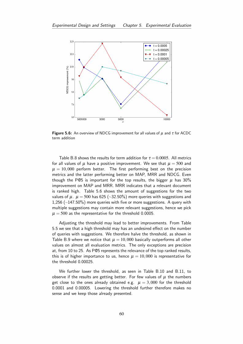
Experimental Design and Settings Chapter 5. Experimental Evaluation
Figure 5.6: An overview of NDCG improvement for all values of µ and τ for ACDCterm addition
Table B.8 shows the results for term addition for τ = 0.0005. All metricsfor all values of µ have a positive improvement. We see that µ = 500 andµ = 10,000 perform better. The first performing best on the precisionmetrics and the latter performing better on MAP, MRR and NDCG. Eventhough the P@5 is important for the top results, the bigger µ has 30%improvement on MAP and MRR. MRR indicates that a relevant documentis ranked high. Table 5.6 shows the amount of suggestions for the twovalues of µ. µ = 500 has 625 (∼32.50%) more queries with suggestions and1,256 (∼147.50%) more queries with five or more suggestions. A query withmultiple suggestions may contain more relevant suggestions, hence we pickµ = 500 as the representative for the threshold 0.0005.
Adjusting the threshold may lead to better improvements. From Table5.5 we see that a high threshold may has an undesired effect on the numberof queries with suggestions. We therefore halve the threshold, as shown inTable B.9 where we notice that µ = 10,000 basically outperforms all othervalues on almost all evaluation metrics. The only exceptions are precisionat, from 10 to 25. As P@5 represents the relevance of the top ranked results,this is of higher importance to us, hence µ = 10,000 is representative forthe threshold 0.00025.
We further lower the threshold, as seen in Table B.10 and B.11, toobserve if the results are getting better. For few values of µ the numbersget close to the ones already obtained e.g. µ = 3,000 for the threshold0.0001 and 0.00005. Lowering the threshold further therefore makes nosense and we keep those already presented.
60

Experimental Design and Settings Chapter 5. Experimental Evaluation
To make the final decision we consider Table 5.6.
t µ Avg. Nr. of Sug. Nr. of Sug 5+ Sug
0.0005 500 30.49 2,548 2,1070.00025 10,000 21.22 2,334 1,429
Table 5.6: Analysis of the number of suggestions for term addition on the candi-dates for the sampled set.
Even though µ = 10,000, for the threshold 0.00025, has higher percentagesof improvement, µ = 500, for the threshold 0.0005, has 214 (∼9.2%) morequeries with suggestions and 678 (∼47.4%) more queries with five or moresuggestions. As the number of suggestions is much higher, we choose thelower value of µ for the higher threshold as values for term addition for theACDC model. These values of µ and τ performs well on the NDG as shownon Figure 5.6.
5.1.5.3 Parameter Setting Experiment 3: Merged vs Baseline
To determine the threshold τ (described section 3.3.1 and 3.3.2) and thesmoothing parameter µ (described in section 3.1) for the merged W&Z andACDC model, we start with the same values we determined for the ACDCmodel, as explained in section 5.1.5.2. All tables in appendix B.3 show theperformance results of either term substitution or term addition for all µ
(columns) on all metrics (rows) for different values of τ. All results arebased on a five run average with 100 queries in each run. However forcomputation reasons we sample the 100 queries from a subset of all thehard queries. The subset consists of 1,000 queries out of 10,920 (9.16%)which are randomly sampled.
5.1.5.3.1 Term Substitution
Figure 5.7 shows the NDCG percentage improvement (y-axis) for each valueof µ (x-axis). Each line represent a different value of τ.
61

Experimental Design and Settings Chapter 5. Experimental Evaluation
Figure 5.7: An overview of NDCG improvement for all values of µ and τ formerged term substitution
Table B.14 shows the performance of term substitution with the initialτ = 0.005 used in ACDC. Most metric scores for all values of µ has animprovement over the baseline, but the better scores are found for µ =1,000 with scores between 15.81% and 55.62%. Next, we check whethera higher or lower threshold improves performance. Table B.15 and TableB.13 show the results for τ = 0.002 and τ = 0.01 respectively. For the lowerthreshold µ = 3,000 performs best with scores between -9.59% and 26.48%and for the higher threshold µ = 1,000 performs best with scores between4.63% and 47.14%. Table B.12 shoes our final attempt in finding theparameter settings by raising the threshold to τ = 0.05. For this thresholdthe best µ = 3,000 with metric scores between 32.44% and 81.04%. Thisoutperforms the previous best setting of µ = 1,000 for τ = 0.005 on allmetrics except NDCG. We therefore choose µ = 3,000 for τ = 0.05 for themerged Wang & Zhai and ACDC model for term substitution. Looking atFigure 5.7 we see that this is indeed one of the selections performing wellon NDCG.
5.1.5.3.2 Term Addition
Figure 5.8 shows the NDCG percentage improvement (y-axis) for each valuesof µ (x-axis). Each line represent a different value of τ.
62

Experimental Design and Settings Chapter 5. Experimental Evaluation
Figure 5.8: An overview of NDCG improvement for all values of µ and τ formerged term addition
For the determination of the merged approach we choose a thresholdand explore the surrounding values. For term addition we have chosen thelower threshold from ACDC candidates (see section 5.1.5.2), as it producessome good improvements. As the data is reduced, compared to ACDC, asthe result of the scaling, a low threshold may improve the merged approach.Table B.16 shows the different µ-values for the threshold 0.0025. A valueof 500 produces some great improvements with more than 100% for allevaluation metrics, except MAP and P@5. As time was an issue for us at thisstate, we double and halve this threshold and pick the best value of µ found.Increasing the threshold (Table B.17) produces impressive improvements forµ = 3,000 with more than 100% improvement for all metrics and up to a186.32% increase for P@5.
Lowering the threshold leads to Table B.18, which overall performs worsethat the two other thresholds presented. We therefore chooke µ = 3,000and τ = 0.005.
From Figure 5.8 we see that the combination of µ and τ shown is indeedto one performing better on the NDCG metric, however we can see that itspikes. This could illustrate a random selection of queries that performextremely well.
It would have been interesting to explore higher values for the threshold,but time did not allow that.
63

Experimental Design and Settings Chapter 5. Experimental Evaluation
5.1.6 User Evaluation
5.1.6.1 Design of Experiment
As stated in section 2.1.3.2 it is assumed that a change of IR model affectsthe results obtained, from the participants. In our experiment we want toinvestigate if a query, reformulated by either Wang & Zhai’s model, ACDCor the merged model, produces a change in relevance of the results that theoriginal unmodified query does not. Our hypotheses are as following:
• Null hypothesis (H0): There is no change in the relevance of the doc-uments retrieved from Karnov’s search engine when using the querymodifications generated by the Wang & Zhai model.
• Alternative hypothesis (H1): There is a change in the relevance ofthe documents retrieved from Karnov’s search engine when using thequery modifications generated by the Wang & Zhai model.
The same hypotheses apply for the ACDC and the merged model. Hav-ing the hypotheses defined we can identify the dependent and independentvariables of the experiment, which must also be clearly defined, as these areimportant for what we want to measure and how we do it. We have oneindependent variable which is the model applied to change the relevanceof the retrieved documents. Having a single independent variable makes iteasier to tell exactly what changed during the experiment. We also haveonly one dependent variable, which is the result sets the participants chooseamong to be the most relevant to a given query. This is the only measurewe are interested in as we want to get an idea on whether the participantsfind one of the three model’s suggestions more or less relevant.
To define our experiment more clearly we must describe the treatments,units and assignment model. Our treatments are the models we want tocompare. We will be comparing a baseline, being the results retrieved fromKarnov’s search engine on unmodified queries, with the results retrievedwhen applying one of the models. The units of our experiments have beenselected with the one criterion that familiarization with Karnov’s search en-gine is required. Three participants were selected, all found through personalrelations. The assignment of models will be random in the sense that theparticipants are presented to two result sets in the same interface. One tothe right, and one to the left. For each query it will be random if the originalor the reformulated query will be presented right or left in the interface. Adetailed description of the experimental setup is found in section 5.1.6.3.
As we are concerned with a single independent variable and because ofthe limited amount of participants at our disposal, we have a within-groupexperiment. This means that we risk the participants suffering from fatigueif exposed to too many queries. As we only have three participants we willnot be able to be evaluate a significant amount of queries, increasing the
64

Experimental Design and Settings Chapter 5. Experimental Evaluation
risk of Type 1 and Type 2 errors, and may also contribute to misleadingconclusions. We will therefore use the results from the user experimentto complement the automatic evaluation to get an idea on how the modelperforms and if it matches the same conclusions. The results we get from theuser experiment will not, on its own, be able to draw any final conclusionson which model results in the most relevant results. The learning effect willnot be of concern as all treatments will be shown at the same time andthe participants must choose between them. Instead we have systematicerrors to worry about. The user may, from the first few top ranked results,already create an idea on which result set is the most relevant. Lower rankeddocuments may therefore either have less influence or not be considered atall. The validity issues observed in these experiments are discussed in section6.2.2.
5.1.6.2 The Participants
The participants selected for the evaluation are all, as described, requiredto posses a familiarization with Karnov’s search engine. Through personalrelations we have found three persons who have knowledge about the sys-tem either through work or courses at the university. The profiles of theseparticipants are:
Participant 1: Female, 26 years. Uses Karnov’s search engine at work ona daily basis as business law clerk.
Participant 2: Female, 28 years. Studying law at the University of Copen-hagen and familiar with Karnov’s search engine through some coursesat the university.
Participant 3: Male, 28 years. Worked for a public body that enforces theconsumer and competition law and is mainly familiar with Karnov’ssearch engine through some courses at the university when studyinglaw at the University of Copenhagen. The participant is currentlyworking for a venture capital company involved in legal research.
The low number of participants may introduce random errors, as de-scribed in section 2.1.3.2.4, and we are aware of this issue. It is hard tofind expert users in Karnov’s system, so we are limited by this. E.g. if wewanted to crowdsourcing users online, it is not likely that we would be ableto recruit Danish speaking experts in Karnov’s system.
5.1.6.3 The Experimental Setup
Each user will first receive a short introduction to the experiment where wespecify the format of the experiment and ensure the user that we are notevaluating them or their skills (see Appendix A).
65

Experimental Design and Settings Chapter 5. Experimental Evaluation
The users will have to evaluate 20 pairs of result sets each; 10 for termsubstitution and 10 for term addition. Each pair consists of a result set froman original query and a result set from the same query, reformulated by oneof the models. Each pair of result sets is displayed at the same time andthe participant’s task is to determine and choose the one he or she judgeshas the most relevant results. Each of the result pairs will only have theoriginal query as a headline (see Figure 5.9), so the participant knows thetopic of the result sets, and hence the user can try to assess which kind ofdocuments are relevant. The order of the result sets will be random.
Figure 5.9: User interface used for the user experiment to evaluate each of theapproaches. The numbers in squares are not shown on the real site but used asmarkers on this figure for later reference.
If the user cannot determine which result set fits the original query thebest, he or she can choose to select that neither result set fits better orworse than the other. If the user does not know the meaning of a query heor she will be able to skip the query and proceed to a new one. We thereforeneed plenty of backup queries to ensure these will not be exhausted.
The layout shown at Figure 5.9 is a remake of Karnov’s website, theyare used to, as shown at Figure 5.10, where most noise have been removed,such as categories and additional search parameters that can be chosen.Instead we added icons that can be clicked. The left arrow (1) chooses theleft result set and (3) chooses the right one. If the user cannot decide onwhich result set contains the more relevant results (2) shall be clicked. Incase the user does not understand the meaning of the query (4) shall bechosen, which skips the current query. (5) shows the participants how manyqueries have been completed and how many there are in total. This is made
66

Experimental Design and Settings Chapter 5. Experimental Evaluation
to not stress the user and all the time let him or her know the progressmade.
Figure 5.10: The user interface to Karnovs search engine.
For the user evaluation we need to log the choices of the user, which alsoincludes clicks on the cannot-decide button. Skipped queries are not loggedas the result sets of these queries have not been judged. For later improve-ments this information may be useful in identifying vague or meaninglessqueries. To keep the participants anonymous, still having the opportunityto describe each’s behavior, every one of them is assigned an ID number,which is logged along with their actions. Furthermore we store data onwhich queries are the original (alongside the number of words in it), whichare the term substitutions and which are the term additions, used for lateranalysis.
5.1.6.4 Selecting the Queries to Evaluate
We will limit the user evaluation to focus only on hard queries for thefollowing reasons:
• These queries are the most challenging and hence interesting for queryreformulation methods, explained in section 5.1.2.
• Hard queries provided the best results in the automatic evaluation(see section 5.2.3.1), and it will therefore be interesting to see if theusers agree with the automatic evaluation results.
67
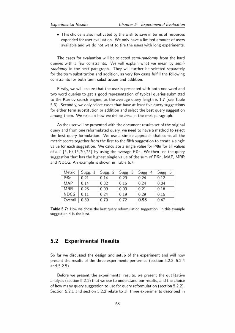
Experimental Results Chapter 5. Experimental Evaluation
• This choice is also motivated by the wish to save in terms of resourcesexpended for user evaluation. We only have a limited amount of usersavailable and we do not want to tire the users with long experiments.
The cases for evaluation will be selected semi-randomly from the hardqueries with a few constraints. We will explain what we mean by semi-randomly in the next paragraph. They will further be selected separatelyfor the term substitution and addition, as very few cases fulfill the followingconstraints for both term substitution and addition.
Firstly, we will ensure that the user is presented with both one word andtwo word queries to get a good representation of typical queries submittedto the Karnov search engine, as the average query length is 1.7 (see Table5.3). Secondly, we only select cases that have at least five query suggestionsfor either term substitution or addition and select the best query suggestionamong them. We explain how we define best in the next paragraph.
As the user will be presented with the document results set of the originalquery and from one reformulated query, we need to have a method to selectthe best query formulation. We use a simple approach that sums all themetric scores together from the first to the fifth suggestion to create a singlevalue for each suggestion. We calculate a single value for P@n for all valuesof n ∈ {5,10,15,20,25} by using the average P@n. We then use the querysuggestion that has the highest single value of the sum of P@n, MAP, MRRand NDCG. An example is shown in Table 5.7.
Metric Sugg. 1 Sugg. 2 Sugg. 3 Sugg. 4 Sugg. 5
P@n 0.21 0.14 0.29 0.24 0.12
MAP 0.14 0.32 0.15 0.24 0.04
MRR 0.23 0.09 0.09 0.21 0.16
NDCG 0.11 0.24 0.19 0.29 0.15
Overall 0.69 0.79 0.72 0.98 0.47
Table 5.7: How we chose the best query reformulation suggestion. In this examplesuggestion 4 is the best.
5.2 Experimental Results
So far we discussed the design and setup of the experiment and will nowpresent the results of the three experiments performed (section 5.2.3, 5.2.4and 5.2.5).
Before we present the experimental results, we present the qualitativeanalysis (section 5.2.1) that we use to understand our results, and the choiceof how many query suggestion to use for query reformulation (section 5.2.2).Section 5.2.1 and section 5.2.2 relate to all three experiments described in
68

Experimental Results Chapter 5. Experimental Evaluation
section 5.2.3 - 5.2.5.
5.2.1 Qualitative Analysis
For each experiment we show the results and perform a qualitative analysisof the query reformulation suggestion generated each time. First we take alook at the top-10 most improved queries and then the top-10 most hurtqueries compared to the baseline using the MAP metric scores. Finally weshow the top most substituted or added terms.
To create a top-10 list we must first define how we measure improvementof a single query in case where either the original or the reformulated queryhas 0 as MAP score. To avoid infinite improvement or decline we simplyignore these cases when computing the top-10 lists. This means that thebest possible improvement would be improving an original query with 1relevant document on rank 25 (MAP: 1/25) to having 1 relevant documenton rank 1 (MAP: 1/1). That would mean a maximum improvement of2400%. The top-lists are further generated based on a random subset of500 queries.
Each row shown for the qualitative analysis contain a query in Danish(as the original data is Danish) with an English translation beneath. Wetranslate as best as we can and use an online Danish-English dictionary 4.
5.2.2 Number of Query Suggestions
Following Wang & Zhai, we evaluate the query suggestions for differentnumbers of suggestions m to a query. If the most relevant documents arereturned when only considering one suggestion to a query, that suggestionis the best possible. When considering two or more suggestions we evaluateeach of the suggestions and pick the best one. This way we can compareeach value of m and locate where it starts not to produce further improve-ment. Let us assume that we do not observe an improvement from m = 4.This tells us that the best suggestion is generally found within the first foursuggestions, which is pretty fine. This corresponds to the user having toexamine up to four suggestions for the optimal query suggestion, which weassume is manageable. For instance, in Google’s current settings they showexactly 4 suggestions, which supports this assumption (see figure 5.11).
4http://ordbog.gyldendal.dk/
69

Experimental Results Chapter 5. Experimental Evaluation
Figure 5.11: Screenshot of a Google search with 4 suggestions. Taken on14/06/2013.
Figure 5.12 and Figure 5.13 show graphs of the different evaluationmetrics (y-axis) and how they perform for different values of m (x-axis),for term substitution and addition respectively. For each value of m, 100random queries were chosen and the average of these are used. For termaddition we evaluated up to a value of m = 20 which means 2,000 randomlyselected queries.
All values of m have at least one suggestion and therefore we can usethe average of all these values for m = 1. We then have the average of2,000 queries instead of 100. For m = 2 we will have (20−1) ·100 = 1,900queries and so on. This means the data for low values of m is very smoothand precise, but as the m-value increases less data is considered making thegraphs more uneven and unprecise.
5.2.2.1 Term Substitution
Looking at all the graphs for term substitution we notice that Wang &Zhai’s model performs better than the baseline for all values of m on allmetrics (Figure 5.12). For P@n the score keeps improving until m reaches13-15, for MRR at m = 13, for MAP at m = 10 and for NDCG at m = 15.
5.2.2.2 Term Addition
Looking at all the figures for term addition (see Figure 5.13) we first noticethat Wang & Zhai’s model performs better than the baseline for all valuesof m. For P@n the score stops improving at 8-9 suggestions, dependingon the value of N. MAP peaks at m = 16, MRR at m = 15 and NDCG atm = 18.
70

Experimental Results Chapter 5. Experimental Evaluation
Figure 5.12: Comparing the best metric scores of the top m recommended queriesby term substitution.
71

Experimental Results Chapter 5. Experimental Evaluation
Figure 5.13: Comparing the best metric scores of the top m recommended queriesby term addition.
Overall for term substitution and term addition the scores peak withinthe range m = 8−18. However, giving the user this many query suggestionsto choose from might be overwhelming, and we therefore choose to set m to5. Wang & Zhai reported m = 3 for P@5. Why our results are inconsistentwith their findings would be interesting to investigate further, but it is notwithin the scope of this thesis. It could however be due to the differences
72

Experimental Results Chapter 5. Experimental Evaluation
in general search and law search domains.
5.2.3 Experiment 1: W&Z vs Baseline
In this section we present the experimental results of Wang & Zhai’s ap-proach (presented in Chapter 3). Section 5.2.3.1 presents the overall resultsof the automatic evaluation, section 5.2.3.2 presents the user evaluationresults and section 5.2.3.3 does a qualitative analysis of the most improvedqueries and the most hurt queries.
5.2.3.1 Results of Automatic Evaluation
Table 5.8, 5.9, 5.10 and 5.11 show the overall automatic evaluation resultsfor term substitution and addition for both the early and full dataset. Thecolumns represent which query difficulty are evaluated (easy, medium orhard), while the rows represent each evaluation metric. Each cell showsboth the metric score for the baseline (original query) and the reformulatedquery with the percentage improvement in parentheses.
Metrics Easy Queries Medium Queries Hard Queries
[email protected] (Original) 0.0422 (Original) 0.0122 (Original)0.0528 (-54.86%) 0.0264 (-37.29%) 0.0205 (+68.25%)
[email protected] (Original) 0.046 (Original) 0.0093 (Original)0.0379 (-48.1%) 0.0242 (-47.46%) 0.0147 (+57.85%)
[email protected] (Original) 0.0438 (Original) 0.0079 (Original)0.0297 (-46.71%) 0.0196 (-55.31%) 0.0114 (+43.85%)
[email protected] (Original) 0.0396 (Original) 0.0074 (Original)0.0253 (-45.66%) 0.0189 (-52.26%) 0.0104 (+41.19%)
[email protected] (Original) 0.0364 (Original) 0.0071 (Original)0.0219 (-45.6%) 0.0172 (-52.65%) 0.0092 (+30.6%)
MRR0.361 (Original) 0.0876 (Original) 0.0337 (Original)0.1503 (-58.36%) 0.0819 (-6.55%) 0.0599 (+77.93%)
MAP0.3464 (Original) 0.0908 (Original) 0.0324 (Original)0.1448 (-58.2%) 0.0813 (-10.52%) 0.0592 (+82.79%)
NDCG0.4723 (Original) 0.1912 (Original) 0.0544 (Original)0.2262 (-52.11%) 0.1452 (-24.05%) 0.0922 (+69.63%)
Table 5.8: Term substitution overall performance for easy, medium and hardqueries on the early dataset for Wang & Zhai’s approach.
73

Experimental Results Chapter 5. Experimental Evaluation
Metrics Easy Queries Medium Queries Hard Queries
[email protected] (Original) 0.0338 (Original) 0.0226 (Original)0.0577 (-50.9%) 0.0328 (-2.76%) 0.0329 (+45.63%)
[email protected] (Original) 0.0373 (Original) 0.0172 (Original)0.0402 (-46.17%) 0.0265 (-28.88%) 0.0241 (+40.22%)
[email protected] (Original) 0.0356 (Original) 0.0146 (Original)0.0309 (-45.78%) 0.0225 (-36.81%) 0.0189 (+29.55%)
[email protected] (Original) 0.0341 (Original) 0.0136 (Original)0.0271 (-43.08%) 0.0202 (-40.67%) 0.0176 (+29.86%)
[email protected] (Original) 0.0325 (Original) 0.013 (Original)0.0233 (-42.25%) 0.0185 (-43.12%) 0.0154 (+18.61%)
MRR0.3676 (Original) 0.0869 (Original) 0.0527 (Original)0.1729 (-52.97%) 0.1003 (+15.33%) 0.0885 (+68.15%)
MAP0.3523 (Original) 0.0875 (Original) 0.0507 (Original)0.17 (-51.75%) 0.1004 (+14.65%) 0.0855 (+68.78%)
NDCG0.4666 (Original) 0.1908 (Original) 0.0824 (Original)0.2468 (-47.1%) 0.174 (-8.76%) 0.1255 (+52.23%)
Table 5.9: Term substitution overall performance for easy, medium and hardqueries on the full dataset for Wang & Zhai’s approach.
Metrics Easy Queries Medium Queries Hard Queries
[email protected] (Original) 0.0148 (Original) 0.0248 (Original)0.0448 (-35.95%) 0.0365 (+146.61%) 0.0636 (+156.63%)
[email protected] (Original) 0.0144 (Original) 0.0172 (Original)0.0299 (-27.76%) 0.0285 (+97.66%) 0.0481 (+179.27%)
[email protected] (Original) 0.0128 (Original) 0.0147 (Original)0.0237 (-22.40%) 0.0249 (+94.25%) 0.0410 (+178.91%)
[email protected] (Original) 0.0108 (Original) 0.0128 (Original)0.0199 (-19.81%) 0.0213 (+97.21%) 0.0358 (+179.10%)
[email protected] (Original) 0.0097 (Original) 0.0113 (Original)0.0171 (-16.72%) 0.0192 (+98.51%) 0.0316 (+179.42%)
MAP0.2435 (Original) 0.0375 (Original) 0.0769 (Original)0.1528 (-37.26%) 0.1129 (+201.06%) 0.1578 (+105.14%)
MRR0.2522 (Original) 0.0366 (Original) 0.0857 (Original)0.1540 (-38.95%) 0.1165 (+218.08%) 0.1736 (+102.52%)
NDCG0.2975 (Original) 0.0757 (Original) 0.1127 (Original)0.2144 (-27.92%) 0.1834 (+142.34%) 0.2315 (+105.46%)
Table 5.10: Term addition overall performance for easy, medium and hard querieson the early dataset for Wang & Zhai’s approach.
74

Experimental Results Chapter 5. Experimental Evaluation
Metrics Easy Queries Medium Queries Hard Queries
[email protected] (Original) 0.0116 (Original) 0.0364 (Original)0.0390 (-19.35%) 0.034 (+192.84%) 0.0703 (+93.08%)
[email protected] (Original) 0.0086 (Original) 0.0232 (Original)0.0257 (-9.04%) 0.0239 (+177.62%) 0.0538 (+131.76%)
[email protected] (Original) 0.0068 (Original) 0.0192 (Original)0.0193 (-5.33%) 0.0199 (+193.16%) 0.0452 (+135.59%)
[email protected] (Original) 0.0061 (Original) 0.0182 (Original)0.0162 (+0.47%) 0.0171 (+180.62%) 0.0391 (+115.10%)
[email protected] (Original) 0.0056 (Original) 0.0170 (Original)0.0143 (+4.84%) 0.0149 (+165.23%) 0.0343 (+101.99%)
MAP0.1923 (Original) 0.0248 (Original) 0.0907 (Original)0.1471 (-23.51%) 0.1016 (+336.11%) 0.1896 (+108.97%)
MRR0.1959 (Original) 0.0245 (Original) 0.1075 (Original)0.1470 (-24.97%) 0.1067 (+309.90%) 0.2103 (+95.65%)
NDCG0.2240 (Original) 0.0488 (Original) 0.1345 (Original)0.2015 (-10.02%) 0.1621 (+232.28%) 0.2611 (+94.15%)
Table 5.11: Term addition overall performance for easy, medium and hard querieson the full dataset for Wang & Zhai’s approach.
Both for term substitution and addition the improvements increased for easyand medium queries between the smaller and bigger data set. For the hardqueries a slight drop in improvement is observed. One explanation is thatsome easy and medium queries are now considered hard, as explained insection 6.1. Table 5.12 illustrates the distribution of queries on the smallerand bigger data set for easy, medium and hard difficulty queries.
Difficulty Early dataset Full dataset
Hard Queries 13,407 (35.40%) 16,821 (40.73%)
Easy Queries 12,623 (33.33%) 12,632 (30.59%)
Medium Queries 11,841 (31.27%) 11,848 (28.69%)
Total Queries 37,871 41,301
Table 5.12: Distribution of the difficulty of queries on the early and full dataset.
The number of hard queries increased by 3,414 while it for easy and mediumbasically did not change. The distribution however changed, which couldindicate that many new hard queries, that were neither easy nor mediumbefore, are added. This does however not corresponds to the improvementincrease for medium and easy queries, as seen in Table 5.9 and Table 5.11.Previous medium and, especially, easy queries which are now hard querieswill have a negative impact on the increase for hard queries as these alreadydo not improve as much. When all these newcomers to the hard difficultyqueries are removed from the easy and medium groups, the two groups are
75

Experimental Results Chapter 5. Experimental Evaluation
obviously under the opposite effect, hence increasing the improvements.
5.2.3.2 Results of User Evaluation
Based on the data collected (available in section C.1) from the user experi-ment (as described in section 5.1.6.3) we extracted information on the votesfrom each participant. Table 5.13 shows how the votes were distributed onthe participants.
Model User 1 User 2 User 3 Overall
Original 16/20 (80.0%) 9/20 (45.0%) 8/20 (40.0%) 33/60 (55.0%)
Wang & Zhai 1/20 (5.0%) 6/20 (30.0%) 6/20 (30.0%) 13/60 (21.7%)
Neither 3/20 (15.0%) 5/20 (25.0%) 6/20 (30.0%) 14/60 (23.3%)
Table 5.13: Distribution of user votes between the original query and the refor-mulated query by the Wang & Zhai approach.
All three favor the result set of the original query over the reformulatedones with 33 votes out of 60. Especially the first participant’s votes onthe original in 16 of the 20 cases are spectacular, as neither of the othertwo come close to this number. They, however, have close to the samedistribution of votes.
Our data also enables us to analyze the distribution of votes on originalqueries of different number of words for either term substitution (Table 5.14)and term addition (Table 5.15).
Model One-worded queries Two-worded queries All queries
Original 4/5 (80.0%) 11/23 (48.8%) 15/28 (53.57%)
W & Z Substitution 0/5 (0.0%) 4/23 (17.4%) 4/28 (14.29%)
Neither 1/5 (20.0%) 8/23 (34.8%) 9/28 (30.03%)
Table 5.14: User evaluation results divided up in one and two-worded originalqueries for Wang & Zhai’s term sustitution.
Model One-worded queries Two-worded queries All queries
Original 18/32 (56.3%) 0/0 18/32 (56.3%)
W & Z Addition 9/32 (28.1%) 0/0 9/32 (28.1%)
Neither 5/32 (15.6%) 0/0 5/32 (15.6%)
Table 5.15: User evaluation results divided up in one and two-worded originalqueries for Wang & Zhai’s term addition.
An interesting observation is that none of the one-worded term substitution
76

Experimental Results Chapter 5. Experimental Evaluation
suggestions received a vote. However the participants could not decide oneight of the cases with two-worded original queries opposed to 11 votes ofthe original for the same number of words. For term addition it is remarkablethat no two-worded queries were a part of the experiment. This issue isdiscussed in section 6.1.
Table 5.16 shows the automatic evaluation metric scores (rows) of thereformulated queries for both term substitution and addition (columns) thatwere evaluated through the user evaluation.
Metric Term Substitution Term Addition
P@5 0.00% -40.00%
P@10 0.00% -12.50%
P@15 0.00% 10.00%
P@20 0.00% 8.33%
P@25 0.00% 15.38%
MRR -27.14% -35.75%
MAP -10.22% -61.18%
NDCG -12.33% 8.28%
Table 5.16: The evaluation metric scores of the user evaluated queries generatedby the Wang & Zhai’s approach.
These result do not reflect and are much lower than the results reportedin Table 5.9 and 5.11 for term substitution and addition. A possible expla-nation for this is discussed in section 6.2.2.
5.2.3.3 Qualitative Analysis of Query Suggestions
In this section we perform a qualitative analysis of the query reformulationsuggestion generated by Wang & Zhai’s approach. Table 5.17 and 5.18 showtop-10 improved and top-10 hurt queries for term substitution. Column 1shows the original query, column 2 the reformulated query and column 3shows the improvement measured in MAP, as explained in section 5.2.1.
As we do not have the required knowledge on juridical terms we havea hard time judging whether a reformulation makes sense in the context.From Table 5.17 we have an example of a query that is changed into some-thing of opposite meaning, though the term substituted fits perfectly in thesame context; the query opsigelse tidsbegrænset lejemal. Both op-
sigelse and aftale fits in the same sentences but have obviously differentmeaning. Substituting one with the other may have a dramatic effect onthe meaning of the query. The query with the highest improvement makesto some extent sense. Marriage and co-ownership can mean the same whenaddressing e.g. joint economy. Still, as mentioned, we may not have the
77

Experimental Results Chapter 5. Experimental Evaluation
necessary knowledge to conclude this.
Original query Reformulated Query Improvement (MAP)
vederlag ægteskab vederlag sameje 2200.00%EN: compensation marriage compensation co-ownership
dødsboskifte skat dødsbo skat 800.00%EN: administration of estate tax estate tax
fristoverskridelse processkrift udeblivelse processkrift 667.74%EN: belated procedural document absence procedural document
ansættelse loyalitet klausul bortvisning loyalitet klausul 637.70%EN: employment loyalty clause expulsion loyalty clause
fond lan uddeling ansvarlig lan uddeling 600.00%EN: Fund loan distribution responsible loan distribution
kassekredit kaution omstødelse kaution 274.69%EN: overdraft surety annulment surety
tabt frifindelse siden tabt frifindelse avance 150.00%EN: lost acquittal since lost acquittal profit
klage indenfor sundhedsvæsenet klage erstatningsadgang sundhedsvæsenet 150.00%EN: complaint within health care complaint compensation health care
retsfortabende passivitet retsfortabende opsigelse 142.07%EN: forfeited passivity forfeited termination
opsigelse tidsbegrænset lejemal aftale tidsbegrænset lejemal 100.00%EN: termination fixed-term lease agreement fixed-term lease
Table 5.17: Top-10 most improved query reformulations by Wang & Zhai’s termsubstitution measured by MAP
Original query Reformulated Query Improvement (MAP)
regres færdselsloven forsikring færdselsloven -90.00%EN: recourse traffic law insurance traffic law
kørekort bedrageri kørekort tyveri -80.00%EN: driver’s license fraud driver’s license theft
ændring visse forbrugeraftaler ændring visse forbruger -75.00%EN: change certain consumer contracts change certain consumer
kæreafgift anke kæreafgift kære -75.00%EN: appeal fee appeal EN: appeal fee appeal
bristede forudsætninger -75.00%EN: shattered EN: assumptions
pant benzin pant forsøg -70.00%EN: deposit gasoline EN: deposit attempt
bekendtgørelse eksplosivstoffer erhvervelse eksplosivstoffer -70.00%EN: proclamation explosives EN: acquisition explosives
overarbejde konkurs overarbejde modregning -65.71%EN: overtime bankruptcy EN: overtime offsetting
kære anke samme sag salær anke samme sag -33.33%EN: appeal appeal same case EN: commission appeal same case
enig anbringender tiltræde anbringender -17.65%EN: agree pleas EN: join pleas
Table 5.18: Top-10 most hurt query reformulations by Wang & Zhai’s termsubstitution measured by MAP
The most improved and hurt queries for term addition are shown inTable 5.19 and Table 5.20.
78

Experimental Results Chapter 5. Experimental Evaluation
Original query Reformulated Query Improvement (MAP)
spil afgift spil 2200.00%EN: game EN: game charge
kontraktsinteresse rente kontraktsinteresse 2000.00%EN: contract interest EN: rate contract interest
dagpenge fradrag dagpenge 1100.00%EN: daily cash benefit EN: deduction daily cash benefit
facebook facebook billeder 1000.00%EN: facebook EN: facebook pictures
funktionærloven handicap funktionærloven 820.11%EN: salaried employees act EN: disability salaried employees act
kaution kaution henstand 750.00%EN: bail EN: bail deferred
entreprenør entreprenør garanti 740.00%EN: entrepreneur EN: entrepreneur guarantee
rekvirentsalær rekvirentsalær konkurs 712.50%EN: consignor fee EN: consignor fee bankruptcy
vandløb offentlige vandløb 687.50%EN: streams EN: public streams
kundeklausul kundeklausul cvr 650.00%EN: solicitation clause EN: solicitation clause cvr
Table 5.19: Top-10 most improved query reformulations by Wang & Zhai’s termaddition measured by MAP
Original query Reformulated Query Improvement (MAP)
private bom private -95.45%EN: private EN: barrier private
afpresning samme afpresning -91.88%EN: blackmail EN: same blackmail
vaben vaben kniv -91.11%EN: weapon EN: weapon knife
udlevering nordisk udlevering -90.00%EN: extradition EN: nordic extradiction
forvaltning begunstigende forvaltning -88.00%EN: management EN: favorable management
design beskyttelse design -87.50%EN: design EN: protection design
ekspropriation byfornyelse ekspropriation -86.97%EN: expropriation EN: city renewal expropriation
selskabsskatteloven selskabsskatteloven afgift -80.59%EN: corporation tax EN: corporation tax charge
markedsføringsloven markedsføringsloven kommentar -78.57%EN: marketing act EN: marketing act comment
mandatar mandatar afskedigelse -78.38%EN: agent EN: agent dismissal
Table 5.20: Top-10 most hurt query reformulations by Wang & Zhai’s termaddition measured by MAP
79

Experimental Results Chapter 5. Experimental Evaluation
The top improved reformulations for term addition do in some cases makeimmediate sense, e.g. the reformulation of facebook into facebook billeder.When Facebook and Instagram changed their terms to basically own allrights to pictures uploaded5, many feared that their pictures would be soldby the companies. This relation explains the large improvement of the query.In Table 5.20 multiple queries, before reformulation, are not specific. Theworst being private which is very general and appears in many differentcontexts. It is therefore really hard to provide meaningful suggestions, thusthe statistically most likely term bom is added.
An analysis of the terms that appears most frequent in the top fivesuggestions can give an idea of which terms affect the improvements themost, as a term occurring often may also be picked as the best suggestionmore often, hence having a bigger impact on the evaluation metric scores.Table 5.21 shows the top terms suggested for query modification for thetop five suggestions for term substitution and addition.
Top substitution terms Top addition terms
konkurs (18.84%) forældelse (3.36%)EN: bankruptcy EN: obsolescence
ansvar (17.88%) ansvar (3.2%)EN: responsibilty EN: responsibility
opsigelse (16.73%) opsigelse (2.82%)EN: termination EN: termination
aftale (15.11%) vold (2.71%)EN: agreement EN: violence
ved (14.31%) konkurs (2.57%)EN: by EN: bankruptcy
mangler (12.5%) bil (2.53%)EN: missing EN: car
bil (11.08%) fast (2.5%)EN: car EN: fixed
leje (10.04%) ved (2.46%)EN: rent EN: by
fast (9.64%) bekendtgørelse (2.46%)EN: fixed EN: decree
passivitet (8.51%) aftale (2.28%)EN: passivity EN: agreement
Table 5.21: Top substitution replacements and top added terms among the top-5query formulation suggestions generated by W&Z.
The term konkurs replaces an original term in 18.84% of the top five sug-gestions, hence the term may have a big impact on the general performanceof the evaluation metrics of term substitution. If it is indeed a term that fit
5Article about the change (in Danish): http://politiken.dk/tjek/digitalt/internet/ECE1846826/instagram-og-facebook-afviser-salg-af-brugernes-billeder/
80

Experimental Results Chapter 5. Experimental Evaluation
in the context this will improve the model, but a term like ved is basicallya stop word and most likely do not contribute to improve a query. For termsubstitution it is the fifth most used term and for addition it is the eighthmost added. As the term intuitively worsen the query and appear as oftenas it does, it may have a big negative impact on the evaluation scores.
5.2.4 Experiment 2: ACDC vs Baseline
In this section we present the experimental results of the ACDC approach(presented in Chapter 4). Section 5.2.4.1 presents the overall results of theautomatic evaluation, section 5.2.4.2 presents the user evaluation resultsand section 5.2.4.3 does a qualitative analysis of the most improved queriesand the most hurt queries.
5.2.4.1 Results of Automatic Evaluation
As described in section 5.1.5.2 the values of µ and τ were determined forterm substitution and addition on a subset of queries. Query reformulationsuggestions for the full set of queries were computed and the experimentrepeated only on hard queries for the values determined. The improvementsfor term substitution on the full set is presented for the different metrics inTable 5.22.
The improvement on the evaluation metrics of ACDC over the baselineranges between 6.47% to 58.83% and performs worse on all metrics exceptP@10 (5.5% improvement) compared to the samples from the subset ofhard queries when the µ and τ was found (see Table B.4). MAP performsa whole 59.84% worse on the full dataset compared to the sampled subset.The drop in performance may be explained by a rather unfortunate randomsampling of the subset, causing the high improvement scores
It is interesting to notice that both the full set and subset have com-parably high values for P@5 and MRR. One possible explanation for thiscould be that generating terms for substitution or addition from clickeddocuments could push some of these clicked documents to a top-5 positionas the query become more specific. At the same time, specifying the querylike this might also push other clicked documents to a lower ranking, whichcould be an explanation why the other P@n scores are lower.
81

Experimental Results Chapter 5. Experimental Evaluation
Metric Improvement
[email protected] (Original)0.0169 (+58.83%)
[email protected] (Original)0.0151 (+50.58%)
[email protected] (Original)0.013 (+21.89%)
[email protected] (Original)0.0114 (+13.78%)
[email protected] (Original)0.01 (+6.47%)
MAP0.0261 (Original)0.0304 (+16.26%)
MRR0.035 (Original)0.0493 (+40.73%)
NDCG0.0604 (Original)0.0765 (+26.7%)
Table 5.22: Term substitution run on the full dataset for ACDC, for µ = 500 andτ = 0.005.
The improvements for term addition on the full set is presented for thedifferent metrics in Table 5.23.
Metric Improvement
[email protected] (Original)0.0386 (+120.54%)
[email protected] (Original)0.0277 (+136.51%)
[email protected] (Original)0.0228 (+148.29%)
[email protected] (Original)0.0195 (+151.36%)
[email protected] (Original)0.017 (+141.13%)
MAP0.0394 (Original)0.0631 (+60.38%)
MRR0.0631 (Original)0.1144 (+81.31%)
NDCG0.0799 (Original)0.1565 (+95.86%)
Table 5.23: Term addition run on the full dataset for ACDC, for µ = 500 andτ = 0.0005.
82

Experimental Results Chapter 5. Experimental Evaluation
Improvements can be seen on all metrics with up to 151.36% improvementon the P@20 metric. Lowest improvement is MAP with an increase of60.38%. When we compare to the numbers computed from the sample(Table B.8) we notice that all values dropped with up to 20% on mostmetrics, except for P@10-P@25, which increased. This may be caused by thenature of random sampling. Table 5.23 should have the best representationof real improvements.
The precision metrics have, compared to the remaining metrics, a ratherbig improvement. This indicates that the ranking of relevant documents ingeneral is higher, which make the lower MRR improvement interesting. Asthe number of relevant documents increase it is expected that the firstrelevant document found also ranks higher. However the lower increase inMRR does not corresponds with this. A possible explanation would be thatlower ranked relevant retrieved documents enters the bottom of the limitof a precision metric, e.g. a search result set has a relevant document atrank six for the original search engine. After reformulating the query therelevant document has rank five, which is just enough to improve P@5 by alot, since it did not contain any relevant documents for the original query.However, as the rank only changes one position, MRR do not increase asmuch.
5.2.4.2 Results of User Evaluation
The complete list of votes can be seen in section C.2. The number ofvotes on the original query, the reformulated query or neither in the userexperiment, as described in section 6.2.2, for the ACDC approach are shownin Table 5.24.
Model User 1 User 2 User 3 Overall
Original 9/20 (45.00%) 10/20 (50.00%) 6/20 (30.0%) 25/60 (41.67%)
ACDC 6/20 (30.00%) 4/20 (20.00%) 7/20 (35.0%) 17/60 (28.33%)
Neither 5/20 (25.00%) 6/20 (30.00%) 7/20 (35.0%) 18/60 (23.30%)
Table 5.24: Distribution of user votes between the original query and the refor-mulated query by the ACDC approach.
Overall the original queries received the most votes, which is of no surpriseas will be discussed in section 6.2.2. Interesting is it that a single participantchose the result set retrieved from the modified query over the original one.That we did not see in the first experiment.
Additional analysis on the results lead to Table 5.25 and Table 5.26,showing the number of votes on term substitution and addition respectively,split up in original query length.
83

Experimental Results Chapter 5. Experimental Evaluation
Model One-worded queries Two-worded queries All queries
Original 4/7 (57.14%) 10/18 (55.56%) 14/25 (56.00%)
ACDC Substitution 1/7 (14.29%) 3/18 (16.67%) 4/25 (16.00%)
Neither 2/7 (28.57%) 5/18 (27.78%) 7/25 (28.00%)
Table 5.25: User evaluation results divided up in one and two-worded originalqueries for ADCD’s term sustitution.
Model One-worded queries Two-worded queries All queries
Original 11/35 (31.43%) 0/0 11/35 (31.43%)
ACDC Addition 13/35 (37.14%) 0/0 13/35 (37.14%)
Neither 11/35 (31.43%) 0/0 11/35 (31.43%)
Table 5.26: User evaluation results divided up in one and two-worded originalqueries for ACDC’s term addition.
It is interesting to see how the term addition gets such a high percentage ofvotes compared to term substitution. As will be discussed in section 6.2.1this can be caused by one worded queries being more ambiguous. Addingsomething to one term may therefore clarify what information is relevant tothe user. When replacing a one worded query it may happen that the newterm does not have the same meaning. It is also interesting that queries witha term added have more votes than original queries. That the participantscould not decide on the most relevant result set in approximately one thirdof all queries tells that the reformulated queries are close to as relevant asthe original ones.
Table 5.27 shows the automatic evaluation metric scores (rows) of thereformulated queries for both term substitution and addition (columns) thatwere evaluating through the user evaluation.
Metric Term Substitution Term Addition
P@5 0.00% 200.00%
P@10 400.00% 175.00%
P@15 807.14% 95.83%
P@20 421.43% 118.52%
P@25 292.86% 143.98%
MRR 636.26% 151.15%
MAP 561.42% 145.39%
NDCG 238.49% 134.10%
Table 5.27: The evaluation metric scores of the user evaluated queries generatedby the ACDC approach.
84

Experimental Results Chapter 5. Experimental Evaluation
The result of term substitution do not reflect and are much higher thanthe results reported in Table 5.22. A possible explanation for this is will bediscussed in section 6.2.2. For term addition the automatic metric resultsare in the same order of magnitude as the ones calculated for the whole setin table 5.23.
5.2.4.3 Qualitative Analysis of Query Suggestions
For term substitution the top 10 most improve query reformulations for therandom sample we picked from the full set of hard queries, and the top 10most hurt hard queries are listed in Table 5.28 and Table 5.29 respectively.
Original query Reformulated Query Improvement (MAP)
opsættende virkning kære ansvar virkning kære 950.00%EN: suspensive effect appeal EN: responsibility effect appeal
uberettiget bortvisning arbejde bortvisning 900.00%EN: unjustified dismissal EN: work dismissal
inddrivelse skatter afgifter inddrivelse skatter leje 381.25%EN: recovery tax charges EN: recovery tax rent
administration ældreboliger modregning ældreboliger 250.00%EN: administration senior housing EN: offsetting senior housing
omlevering forbrugerkøb mangler forbrugerkøb 200.00%EN: redelivery consumer goods EN: missing consumer goods
statens tjenestemænd grønland statens afskedigelse grønland 187.58%EN: state officials Greenland EN: state dismissal Greenland
deling pensioner ægtepagt pensioner 157.14%EN: sharing pensions EN: prenuptial pensions
drives forretningsmæssigt dsb selskabets forretningsmæssigt dsb 150.00%EN: operated commercially dsb EN: company commercially dsb
udøve konkurs opsigelse konkurs 125.00%EN: exercise bankruptcy EN: cancellation bankcruptcy
virke dørmænd rette dørmænd 91.94%EN: work doorman EN: appropriate doorman
Table 5.28: Top-10 most improved query reformulations by ACDC’s term substi-tution measured by MAP
It is really hard for us to determine if the reformulated queries are asgood or bad. The reformulation of deling pensioner into ægtepagt
pensioner does in some way make sense, while the suggestion arbejde
bortvisning to the original query uberettiget bortvisning is hard tojudge; and both are in the list of most improved queries. From the list ofmost hurt queries most do not make immediate sense to us, however thata query like leasing anbragt has a negative impact compared to lease
anbragt as they share the same meaning. This may happen due to theterm lease being used more often than leasing in documents.
85

Experimental Results Chapter 5. Experimental Evaluation
Original query Reformulated Query Improvement (MAP)
fejlagtig sagsomkostninger modregning sagsomkostninger -93.33%EN: erroneous legal costs EN: offsetting legal costs
lønmodtageres retsstilling lønmodtageres retsstilling -90.91%virksomhedsoverdragelse afskedigelseEN: employees’ rights business transfer EN: employees’ rights dismissal
patienters retsstilling patienters udlejer -88.57%EN: patients’ rights EN: patients’ landlord
lease anbragt leasing anbragt -80.00%EN: lease placed EN: leasing placed
indsigelse rekonstruktion direkte rekonstruktion -53.85%EN: object reconstruction EN: direct reconstruction
mortifikation retsafgift mortifikation forældremyndighed -44.44%EN: cancellation court fee EN: cancellation custody
fællesbo skifteloven skifte skifteloven -33.33%EN: community property law change EN: change law change
tjener funktionær løn funktionær -15.38%EN: earn/servant officer EN: salary officer
regreskrav spirituskørsel erstatningsansvar spirituskørsel 0.00%EN: recourse drunk driving EN: liability drunk driving
arveret arv 0.00%EN: inheritance rights EN: inheritance
Table 5.29: Top-10 most hurt query reformulations by ACDC’s term substitutionmeasured by MAP
For term addition the top 10 most improve query reformulations for therandom sample we picked from the full set of hard queries, and the top 10most hurt hard queries are listed in Table 5.30 and Table 5.31 respectively.
Original query Reformulated Query Improvement (MAP)
konkursregulering konkursregulering sale 2400.00%EN: bankruptcy regulation EN: bankruptcy regulation halls
forordningen bruxelles forordningen 2300.00%EN: regulation EN:Brussels regulation
beskikkelse beskikkelse advokat 2300.00%EN: bribery EN: bribery lawyer
opfindelser opfindelser forskningsinstitutioner 2200.00%EN: inventions EN: inventions research institutions
steen steen rønsholdt 2000.00%EN: steen EN: steen rønsholdt
lønmodtageres lønmodtageres retsstilling 1800.00%EN: employees’ EN: employees’ rights
betalingskort aflæsning betalingskort 1800.00%EN: debit card EN: reading debit card
ussing ussing køb 1475.00%EN: ussing EN: ussing buy
ejendomsforbehold forbrugerkøb ejendomsforbehold 1300.00%EN: retention of ownership EN: consumer purchases retention of ownership
aktionær aktionær adgang 1300.00%EN: shareholder EN: shareholder access
Table 5.30: Top-10 most improved query reformulations ACDC’s by term additionmeasured by MAP
86

Experimental Results Chapter 5. Experimental Evaluation
Original query Reformulated Query Improvement (MAP)
færdsel tæt færdsel -96.00%EN: traffic EN: close traffic
frakendelse ubetinget frakendelse -96.00%EN: suspension EN: unconditional suspension
forvaltningslovens forvaltningslovens partsbegreb -94.12%EN: administrative procedures’ EN: administrative procedures’ part concept
kildeskat indkomstmodtager kildeskat -94.12%EN: withholding tax EN: income earner withholding tax
færdselslovens regres færdselslovens -93.75%EN: road traffic act EN: recourse road traffic act
skattekontrolloven skattekontrolloven mulighed -93.33%EN: tax control act EN: tax control act opportunity
grundloven fortolkning grundloven -92.86%EN: constitution EN: interpretation constitution
købelov nordisk købelov -92.31%EN: sales law EN: nordic sales law
byggeloven pabud byggeloven -91.67%EN: building act EN: injunction building act
betalingstjenester visse betalingstjenester -91.30%EN: payment services EN: certain payment services
Table 5.31: Top-10 most hurt query reformulations by ACDC’s term additionmeasured by MAP
As already mentioned, it is really hard for us to determine if the reformu-lated queries are as good or bad as the numbers say, e.g. the term steen (aforename) has rønsholdt (a surname) added and yields 2000% improve-ment. We have no knowledge on whether the most interesting steen is therønsholdt one, except that our model, built on statistics, says so. Fromthe list of hurt queries we could image that a suggestion such as pabud
købeloven makes sense, however the evaluation metric MAP states other-wise. It is difficult to make a qualified guess on whether this is indeed a badsuggestion to a user of the search engine.
The improvement on some of the changes that at first glance do notcontain much sense to us is caused by queries that have only one relevantdocument, which has rank 25. After the query reformulation a relevantdocument now has rank one. This could happen to rarely written querieswhere possibly only one, or very few, document(s) has been clicked.
As mentioned in section 5.2.3.3 an analysis of the terms that appearsmost frequent in the top five suggestions can give an idea of which terms af-fect the improvements the most. Table 5.32 shows the top terms suggestedfor query modification for the top five suggestions for term substitution andaddition.
87

Experimental Results Chapter 5. Experimental Evaluation
Top substitution terms Top addition terms
leje (18.28%) ændring (1.75%)EN: rent EN: change
ansvar (17.97%) manglende (1.18%)textitEN: responsibility EN: missing
opsigelse (15.9%) betaling (1.09%)textitEN: payment EN: payment
arbejde (15.58%) mellem (1.04%)textitEN: work EN: between
aktier (14.47%) bekendtgørelse (0.99%)textitEN: stocks EN: decree
bil (13.51%) ved (0.95%)textitEN: car EN: by
mangler (13.04%) fast (0.95%)textitEN: missing EN: fixed
modregning (11.45%) visse (0.95%)textitEN: offsetting EN: certain
konkurs (10.81%) forsøg (0.95%)textitEN: bankcruptcy EN: attempt
sagsomkostninger (10.65%) køb (0.95%)textitEN: legal costs EN: buy
Table 5.32: Top substitution replacements and top added terms among the top-5query formulation suggestions generated by ACDC.
The top added terms are mostly very broad terms or terms that we cannotimagine will provide an increase in the meaning of any query. The majorityof the substitute terms do seem to be words that could improve the un-derstanding of a query. Is it however worrying that such high percentagesof the hard queries have these terms in their top five suggestions, as it ishighly unlikely that these terms fits such a high percentage of the queries,and because it may have a high impact on the evaluation scores.
5.2.5 Experiment 3: W&Z + ACDC vs Baseline
In this section we present the experimental results of the merged Wang &Zhai and ACDC approach described in section 4.4. Section 5.2.5.1 presentsthe overall results of the automatic evaluation, section 5.2.5.2 presents theuser evaluation results and in section 5.2.5.3 we analyze the query sugges-tions.
88

Experimental Results Chapter 5. Experimental Evaluation
5.2.5.1 Results of Automatic Evaluation
The term substitution results, on the full set with µ = 3,000 and τ = 0.05,are presented in Table 5.33. As with the term substitution for ACDC theresults are again much lower than the randomly sampled subset for the sameparameter settings in Table B.12. This time the difference in performanceis even greater, which very likely could mean that another parameter settingcould have produced better results, however time prevents us from inves-tigating this further. Once again P@5 and MRR perform comparably well,which again supports the idea that including clicked documents might pushsome of the documents to a high position while other documents do notimprove their ranking much as the query becomes too specific.
Metric Improvement
[email protected] (Original)0.0188 (+20.6%)
[email protected] (Original)0.0138 (+21.03%)
[email protected] (Original)0.0111 (+7.03%)
[email protected] (Original)0.0097 (+1.85%)
[email protected] (Original)0.0085 (+3.93%)
MAP0.0197 (Original)0.0302 (+53.11%)
MRR0.0327 (Original)0.0567 (+73.34%)
NDCG0.0553 (Original)0.0761 (+37.52%)
Table 5.33: Term substitution overall performance for hard queries on the fulldataset for the merged model for µ = 3,000 and τ = 0.05.
Based on the randomly sampled subset of hard queries for term addition,as presented in Table B.17, the values of µ and τ were determined to havethe optimal values of 3,000 and 0.0005 respectively. Using the full set ofhard queries for these values yield the improvements shown in Table 5.34.
89
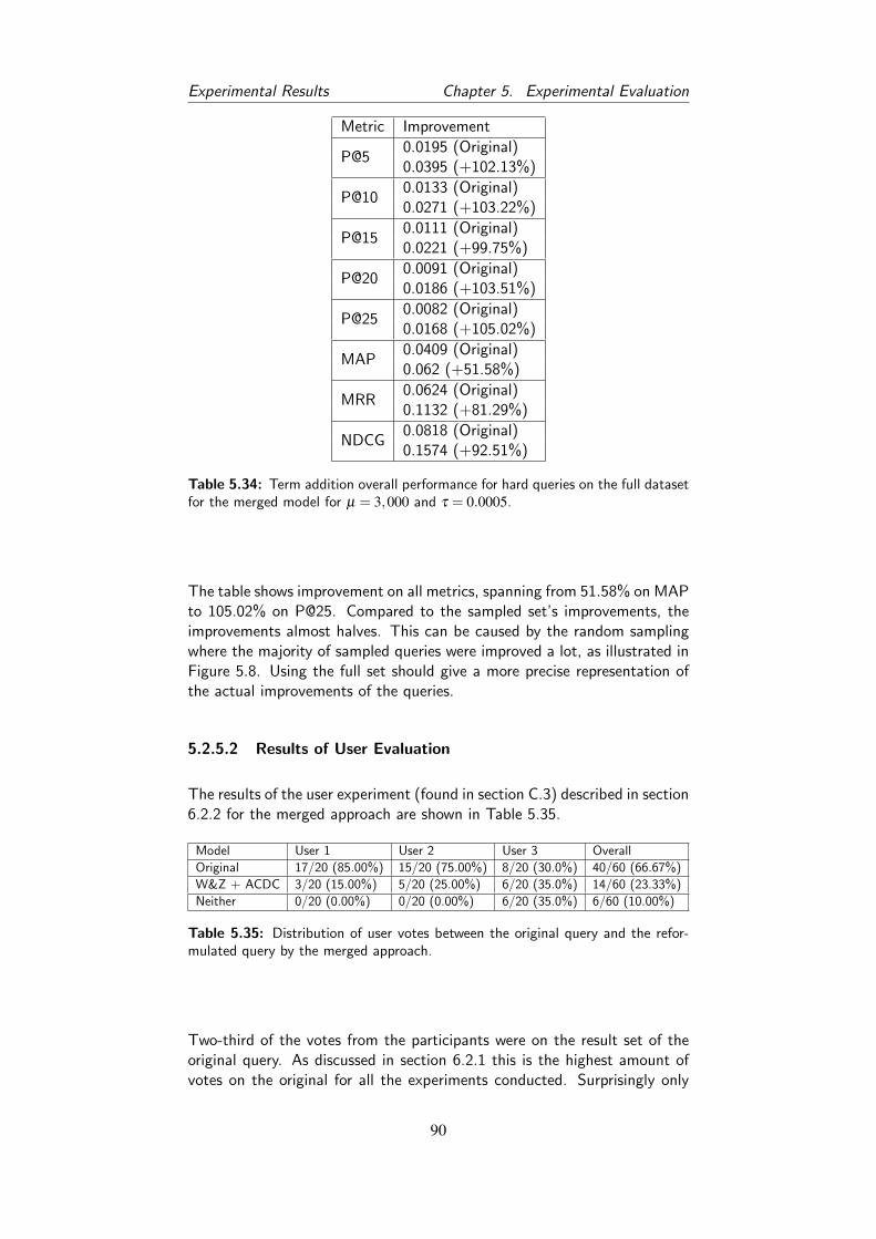
Experimental Results Chapter 5. Experimental Evaluation
Metric Improvement
[email protected] (Original)0.0395 (+102.13%)
[email protected] (Original)0.0271 (+103.22%)
[email protected] (Original)0.0221 (+99.75%)
[email protected] (Original)0.0186 (+103.51%)
[email protected] (Original)0.0168 (+105.02%)
MAP0.0409 (Original)0.062 (+51.58%)
MRR0.0624 (Original)0.1132 (+81.29%)
NDCG0.0818 (Original)0.1574 (+92.51%)
Table 5.34: Term addition overall performance for hard queries on the full datasetfor the merged model for µ = 3,000 and τ = 0.0005.
The table shows improvement on all metrics, spanning from 51.58% on MAPto 105.02% on P@25. Compared to the sampled set’s improvements, theimprovements almost halves. This can be caused by the random samplingwhere the majority of sampled queries were improved a lot, as illustrated inFigure 5.8. Using the full set should give a more precise representation ofthe actual improvements of the queries.
5.2.5.2 Results of User Evaluation
The results of the user experiment (found in section C.3) described in section6.2.2 for the merged approach are shown in Table 5.35.
Model User 1 User 2 User 3 Overall
Original 17/20 (85.00%) 15/20 (75.00%) 8/20 (30.0%) 40/60 (66.67%)
W&Z + ACDC 3/20 (15.00%) 5/20 (25.00%) 6/20 (35.0%) 14/60 (23.33%)
Neither 0/20 (0.00%) 0/20 (0.00%) 6/20 (35.0%) 6/60 (10.00%)
Table 5.35: Distribution of user votes between the original query and the refor-mulated query by the merged approach.
Two-third of the votes from the participants were on the result set of theoriginal query. As discussed in section 6.2.1 this is the highest amount ofvotes on the original for all the experiments conducted. Surprisingly only
90

Experimental Results Chapter 5. Experimental Evaluation
one participant was in doubt of which result set provided the most relevantresults. The six votes from this participant is representative for only 10%of the overall amount of votes.
Additional analysis on the results lead to Table 5.36 and Table 5.37,showing the number of votes on term substitution and addition respectively,split up in original query length.
Model One-worded queries Two-worded queries All queries
Original 5/5 (100.00%) 19/29 (65.52%) 24/34 (70.59%)
W&Z + ACDC Substitution 0/5 (0.00%) 6/29 (20.69%) 6/34 (17.65%)
Neither 0/5 (0.00%) 4/29 (13.79%) 4/34 (11.76%)
Table 5.36: User evaluation results divided up in one and two-worded originalqueries for the merged approach for term substitution.
Model One-worded queries Two-worded queries All queries
Original 16/26 (61.54%) 0/0 16/26 (61.54%)
W&Z + ACDC Addition 8/26 (30.77%) 0/0 8/26 (30.77%)
Neither 2/26 (7.69%) 0/0 2/26 (7.69%)
Table 5.37: User evaluation results divided up in one and two-worded originalqueries for the merged approach for term addition.
It is interesting to see that no one-worded queries for substitution havebeen selected, and that in only six of the 29 cases of two-worded queriesthe substitution was picked.
Table 5.38 shows the automatic evaluation metric scores (rows) of thereformulated queries for both term substitution and addition (columns) thatwere evaluated through the user evaluation.
Metric Term Substitution Term Addition
P@5 60.00% 0.00%
P@10 106.90% 50.00%
P@15 125.35% 50.00%
P@20 184.21% 50.00%
P@25 255.56% 50.00%
MRR 31.52% -31.75%
MAP 57.10% -35.43%
NDCG 67.23% 406.86%
Table 5.38: The evaluation metric scores of the user evaluated queries generatedby the merged approach
91

Experimental Results Chapter 5. Experimental Evaluation
The results of term substitution and addition do not reflect the resultsreported in Table 5.33 and 5.34 respectively. Some values are much smaller,some much bigger and some are in the same order of magnitude. A possibleexplanation for this is discussed in section 6.2.2.
5.2.5.3 Qualitative Analysis of Query Suggestions
From the random samples of hard queries for the full set we extracted the10 most improved queries and the 10 most hurt ones, as presented in Table5.39 and Table 5.40.
Original query Reformulated Query Improvement (MAP)
inddrivelse skatter afgifter sagsomkostninger skatter afgifter 1410.45%EN: recovery tax charges EN: legal costs tax charges
varsling afskedigelser større opsigelse afskedigelser større 1400.00%EN: warning dismissals larger EN: cancellation dismissals larger
lars lindencrone rekonstruktion lars lindencrone virksomhedsoverdragelse 904.78%EN: lars lindencrone rekonstruktion EN: lars lindencrone company transfer
uberettiget bortvisning godtgørelse bortvisning 900.00%EN: unjustified dismissal EN: dispensation dismissal
ægtefælle skifteloven pension skifteloven 550.00%EN: spouse estate act EN: pension estate act
udgifter uddannelse fradragsberettiget udgifter mangler fradragsberettiget 400.00%EN: cost education deductible EN: cost missing deductible
andelsbolig fremleje andelsbolig opsigelse 250.00%EN: cooperative housing sublease EN:cooperative housing termination
misbrug uskiftet bo misbrug skifte bo 188.00%EN: abuse unchanged stay EN: abuse change stay
forsøgt voldtægt mindrearig forsøgt vold mindrearig 175.00%EN: attempted rape minor EN: attempted violence minor
billede samtykke reklame indhentet samtykke reklame 166.67%EN: photo consent advertisement EN: obtained consent advertisement
Table 5.39: Top-10 most improved query reformulations by term substitutionmeasured by MAP generated by the merged approach.
As explained in section 5.2.3.3 and section 5.2.4.3 it is hard to figure outwhether a term replaced makes more sense than the original term or not, aswe do not ourselves possess the required knowledge to make this judgment.The query improved the most is inddrivelse skatter afgifter whichat first glance does not corresponds to the reformulated sagsomkostninger
skatter afgifter. There could, however, be a relation between the twothat we do not fully understand. In Table 5.40 the most hurt queries areshown. It is not hard to agree on the negative improvement on some ofthese, e.g. the query indsmugling. It is modified into kokain. Though thetwo terms may often appear together and make sense in the same sentence,they obviously do not share the same meaning. indsmugling could berelated to any type of drugs, immigrants, cars, endangered animals etc.
92

Experimental Results Chapter 5. Experimental Evaluation
Original query Reformulated Query Improvement (MAP)
børns retsstilling børns ophævelse -91.67%EN: children’s rights EN:
honorar skønsmand erstatningsansvar skønsmand -89.09%EN: fee qualified valuer EN: liability qualified valuer
kæreafgift anke kæreafgift kære -75.00%EN: appeal fee appeal EN: appeal fee appeal
aremal varsel aremal ophævelse -71.55%EN: term of years notice EN: term of years repeal
byggetilladelse anvendes byggetilladelse ændring -70.83%EN: building permit used EN: building permit change
indsmugling kokain -69.39%EN: smuggling EN: cocaine
betinget udvisning fængsel udvisning -67.62%EN: suspended expulsion EN: imprisoned expulsion
bedrageri dankort fængsel dankort -63.64%EN: fraud credit card EN: prison credit card
skattefri virksomhedsomdannelse fonde virksomhedsomdannelse -62.67%EN: tax free business transformation EN: fund business transformation
førerret udenlandsk kørekort førerretten udenlandsk kørekort -61.54%EN: entitlement to drive foreign EN: the entitlement to drivedriving license foreign driving license
Table 5.40: Top-10 most hurt query reformulations by term substitution measuredby MAP generated by the merged approach.
The 10 most improved and 10 most hurt queries for term addition canbe seen in Table 5.41 and Table 5.42.
Original query Reformulated Query Improvement (MAP)
konkursregulering konkursregulering sale 2400.00%EN: bankruptcy regulation EN: bankruptcy regulation halls
forordningen bruxelles forordningen 2300.00%EN: regulation EN: Brussels regulation
beskikkelse beskikkelse advokat 2300.00%EN: bribery EN: bribery laywer
steen steen rønsholdt 2000.00%EN: steen EN: steen rønsholdt
lønmodtagere lønmodtagere ret 1800.00%EN: employees EN: employees rights
aktionær aktionær adgang 1300.00%EN: shareholder EN: shareholder access
dagbøder dagbøder forsinkelse 1150.00%EN: daily fine EN: daily fine delayal
kvalificeret kræver kvalificeret 1120.41%EN: qualified EN: demand qualified
føtex føtex tørklæde 1050.00%EN: føtex EN: føtex headscarf
forbrugerkøb forbrugerkøb handelskøb 1050.00%EN: consumer goods EN: consumer goods commerce purchases
Table 5.41: Top-10 most improved query reformulations by term addition mea-sured by MAP generated by the merged approach.
93

Experimental Results Chapter 5. Experimental Evaluation
Original query Reformulated Query Improvement (MAP)
frakendelse ubetinget frakendelse -96.00%EN:disqualification EN: unconditional disqualification
forvaltningslovens forvaltningslovens partsbegreb -94.12%EN: administrative procedure’s EN: administrative procedure’s part concept
elforsyning elforsyning ved -93.75%EN: electricity supply EN: electricity supply by
færdselslovens regres færdselslovens -93.75%EN: the road traffic act’s EN: recourse the road traffic act’s
jernbane luftfart jernbane -92.31%EN: rail EN: aviation rail
dørmand virke dørmand -92.00%EN: doorman EN: work doorman
skel hegn skel -91.67%EN: difference EN: fence difference
betalingstjenester visse betalingstjenester -91.30%EN: payment services EN: certain payment services
grundloven interesse grundloven -90.91%EN: constitution EN: interest constitution
fiskeri fiskeri gentagelse -90.91%EN: fishing EN: fishing repetition
Table 5.42: Top-10 most hurt query reformulations by term addition measuredby MAP generated by the merged approach.
An immediate observation is that term addition provides really large im-provements on the top improved queries, but also very low numbers for themost hurt ones. It is interesting that the query suggestion føtex tørk-
læde to the original query føtex improve by 1050%. This indicates thatmost relevant documents regarding Føtex may refer to the Føtex Case6,which was a case on a former employee of Føtex who was fired as a resultof requiring to wear a scarf.
As first mentioned in section 5.2.3.3 the analysis of the terms thatappears most frequent in the top five suggestions can be used in order toidentify which terms affect the improvements the most. Table 5.43 showsthe top terms suggested for query modification for the top five suggestionsfor term substitution and addition.
6Føtex Case overview (in Danish): http://www.bt.dk/nyheder/det-handler-foetex-sagen-om
94

Experimental Results Chapter 5. Experimental Evaluation
Top substitution terms Top addition terms
leje (25.4%) ved (3.59%)EN: rent EN: by
opsigelse (24.67%) ændring (3.46%)EN:cancellation EN: change
sagsomkostninger (21.34%) vold (2.5%)EN: legal costs EN: violence
modregning (17.42%) opsigelse (2.5%)EN: offsetting EN: cancellation
omstødelse (15.24%) bil (2.18%)EN: annulment EN: car
udlæg (14.51%) fast (2.11%)EN: outlay EN: fixed
mangler (14.51%) salg (1.92%)EN: missing EN: sale
ophævelse (9.14%) privat (1.92%)EN: repeal EN: private
tyveri (8.56%) køb (1.86%)EN: theft EN: buy
tab (8.13%) manglende (1.79%)EN: loss EN: missing
Table 5.43: Top substitution replacements and top added terms among the top-5query formulation suggestions generated by the merged approach.
As seen the term ved appears first on the list of most frequent added termsin the top five suggestions for hard queries on the sample of the full set.This term does, as discussed in section 5.2.3.3, most likely not contributewith any meaningfulness. Still it is the most common term added.
95

In theory, there is no difference between theory andpractice, but not in practice.
Unknown
6Discussion
In the previous chapter we evaluated experimentally Wang & Zhai’s ap-proach 5.2.3, our ACDC approach 5.2.4 and both approaches merged 5.2.5through automatic and user evaluation.
The user evaluation did not draw the same conclusions as the automaticevaluation on the randomly selected hard queries. Instead it opposes theresults and shows a worsening of the relevance of the results retrieved byKarnov’s search engine when using query reformulation compared to theoriginal queries. It is a known fact that automatic and user evaluationperformance does not always correspond to each other. Kelly et al. [21] in-vestigated this difference further by studying which factors affect the users’evaluation ratings. We will now discuss the results of the automatic evalu-ation in section 6.1 and user evaluation in section 6.2.1 and the mismatchbetween the conclusions of them. We will further discuss each of the threequery reformulation models in section 6.3.
6.1 Automatic Evaluation
In this section we will reflect upon the results obtained from automaticallyevaluating the three models, Wang & Zhai (chapter 3), ACDC (chapter4), and the combination of both (section 4.4), with the evaluation metricsexplained in section 2.1.3.1.3. The results from the automatic evaluation ispresented in section 5.2.3.1, 5.2.4.1, and 5.2.5.1 for Wang & Zhai, ACDCand the merged version respectively.
Time did not allow us to analyze the performance of queries of easyand medium difficulty for other Wang & Zhai’s approach (section 5.2.3.1).
96

Automatic Evaluation Chapter 6. Discussion
We expected the model to work better the more difficult a query is, whichindeed appears to be the case for term substitution (Table 5.8 and Table5.9), but unexpected is it that medium queries outperforms hard queries forterm addition (Table 5.10 and Table 5.11), especially on the bigger dataset.
General for all of the automatic evaluation results for each of the ap-proaches is that the term addition performed better than the term substitu-tion on every metric. One of the reasons for this could be that the parametersettings for the term addition is closer to the optimal settings compared tothe parameter settings of the term substitution. Although we tried to findthe optimal settings for the smoothing parameter µ and threshold τ, timeonly allowed us to test 3-4 different values for τ and five values between500 and 10,000 for µ. Another reason could also lie in the difference inthe problem term substitution and term addition tries to solve. Term sub-stitution deals with the problem of vaguely formulated queries while termaddition deals with underspecified queries. It is not unlikely that addinga term to a query, rather than substituting a term, could produce betterevaluation results especially for short queries. Almost all queries that termaddition finds at least five query suggestion for are only one-word querieswhich seems like the perfect candidates that would benefit from adding aterm to.
Another interesting observation is that the results of the automatic eval-uation for the Wang & Zhai approach are comparable with the results of ourACDC approach. For term substitution ACDC performs better for P@5 andP@10 than Wang & Zhai by 10.36% to 13.20% while it performs worse forthe other metrics by 7.66% to 51.89%. Furthermore, term addition ACDCperforms better on P@5, P@10, P@15, P@20, P@25, NDCG than Wang &Zhai by 1.71% to 39.14% while it perform worse on MAP and MRR with14.34% to 48.59%. Generally term substitution works a little better onWang & Zhai’s approach while term addition works a little better for ACDCwhich on a whole makes the two approaches comparable.
It is noteworthy that only one-worded queries have been selected forterm addition. That the amount of hard multi-worded queries with at leastfive suggestions are so few may be caused by a too high threshold, though wealready limited our thresholds in section 5.1.5.1, 5.1.5.2, 5.1.5.3 for Wang& Zhai’s model, ACDC and the merged model respectively. It can how-ever be explained by one worded queries most likely being more ambiguousthan multi-worded queries, as more terms often means a more concrete andspecified query.
97

User Evaluation Chapter 6. Discussion
6.2 User Evaluation
6.2.1 Results
Based on the numbers presented in section 5.2.3.2, 5.2.4.2 and 5.2.5.2 wediscuss the findings.
Table 5.13 shows how one participant has voted on the result set of theoriginal query more often than the two other participants. One reason couldbe that this participant is the one working with Karnov’s search engine ona daily basis which might have conditioned her. At one point during theevaluation she said“This is such a typical Karnov result set”and chose thatone. Her experience with the system may have gotten her used to the look ofthe results and therefore have a conditioning-driven tendency to pick these.The two other participants with less experience still have an overweight oforiginal query votes, but not in the same degree as participant one.
From Table 5.14, 5.25 and 5.36 we see that term substitution onlyreceived 1 vote out of 17 on suggestions where the original query consistsof a single word. This may be caused by one-worded queries being vagueand the statistically best suited replacement does not always make sense.E.g. the query unge (EN: young one or kid) is replaced with uden (EN:without) which obviously retrieves a whole other set of results, which mostlikely is not connected to each other. In some cases the replacement maymake sense. One example where the user could not decide which resultset was best is føreret (EN: right to drive), which was replaced bykørekort (EN: driver’s license). It may not hurt the original queryin every case, but more often it would have been better to not reformulateone-worded queries by substitution.
The user evaluation results for Wang & Zhai and ACDC are almostidentical for term substitution, however for the merged approach we findboth most votes for the original query and for the reformulated query (seeTable 5.36). A possible reason for this could again be because that usingclicked documents for the contextual models might boost queries and hurtothers because the reformulated query becomes too specific.
Term substitution does in general receive a lot of votes where the par-ticipant cannot decide whether the original query’s result set or the refor-mulated one’s is better. That is 30.03%, 28.00% and 11.76% for Wang &Zhai, ACDC and the merged approach respectively. This indicates that termsubstitution does indeed produce suggestions that are similar to the originalsuggestion. However in most cases the original query results was preferredfor all approaches. A likely explanation for this might the experimentalsetup, as will be described in section 6.2.2.
From Table 5.15, 5.26 and 5.37 we see that term addition receivedmore votes than term substitution in all approaches. This could be becausethe threshold for term addition is too high or the threshold for term sub-
98

User Evaluation Chapter 6. Discussion
stitution is too low. In the first case the term addition contributes onlywith statistical highly relevant suggestions. Even though there will be alow amount of queries with corresponding suggestions, we only select thosewith suggestions for the experiment, increasing the quality of those usedfor the evaluation. The term addition suggestions used in the experimentmay therefore have more relevant suggestions, hence increasing the numberof votes. In the other case term substitution may have a low thresholdcomputing suggestions of low relevance, hence obtaining fewer votes.
Another interesting observation is that the users actually preferred thereformulated query by term addition over the original query for the ACDCapproach. In the other approaches the original query was preferred as it waswith term substitution.
One clear difference with the merged approach compared to the otherapproaches is that the users only are undecided for 11.76% and 7.69% ofthe queries for term substitution and term addition respectively. This couldonce again supports the idea that queries are more specific for the mergedapproach making it easier for the user to decide whether the original orreformulated approach is better. For this reason, for both term substitutionand addition, most users preferred the original query from all approaches(70.59% and 61.54% respectively).
6.2.2 Experimental Settings
The findings of the user evaluation can only be seen as an indication. Dueto the low number of participants we cannot give statistical significance tothe finding. Having only three users is not enough to represent the wholeuser base of Karnov’s search engine and will definitely introduce randomerrors as described in section 2.1.3.2.4. Users with the right skills andexperience working with the search engine are sparse and time did not allowus to find more participants. Furthermore it can also be seen through theautomatic evaluation of the set of queries evaluated through user evaluationin table 5.16, 5.27 and 5.38, that the semi-randomly sampled queries do notcorrespond to automatic evaluation results on the whole set. Few of themetric score are in the same order of magnitude, while many are eithermuch higher or much lower than the results reported for the whole set.This must be due to the few numbers of user and queries evaluated byusers. Alternatively the selection of queries used for the user evaluationcould be selected randomly amongst a set of queries that perform withina certain range of the average query performance for the whole set. Thismight make the user evaluated queries more representative of the whole set.
One of the reasons why the user evaluation did not produce as goodresults as the automatic evaluation is a systematical error in the settingof the experiment. The queries selected for the experiment were randomlyselected from the hard test where the query has at least five suggestions.Only the original query was shown to the user and no further information
99
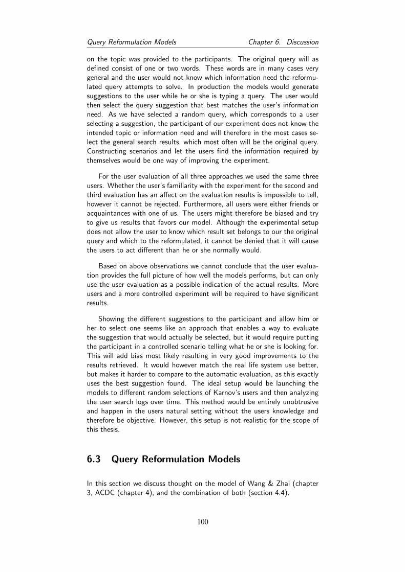
Query Reformulation Models Chapter 6. Discussion
on the topic was provided to the participants. The original query will asdefined consist of one or two words. These words are in many cases verygeneral and the user would not know which information need the reformu-lated query attempts to solve. In production the models would generatesuggestions to the user while he or she is typing a query. The user wouldthen select the query suggestion that best matches the user’s informationneed. As we have selected a random query, which corresponds to a userselecting a suggestion, the participant of our experiment does not know theintended topic or information need and will therefore in the most cases se-lect the general search results, which most often will be the original query.Constructing scenarios and let the users find the information required bythemselves would be one way of improving the experiment.
For the user evaluation of all three approaches we used the same threeusers. Whether the user’s familiarity with the experiment for the second andthird evaluation has an affect on the evaluation results is impossible to tell,however it cannot be rejected. Furthermore, all users were either friends oracquaintances with one of us. The users might therefore be biased and tryto give us results that favors our model. Although the experimental setupdoes not allow the user to know which result set belongs to our the originalquery and which to the reformulated, it cannot be denied that it will causethe users to act different than he or she normally would.
Based on above observations we cannot conclude that the user evalua-tion provides the full picture of how well the models performs, but can onlyuse the user evaluation as a possible indication of the actual results. Moreusers and a more controlled experiment will be required to have significantresults.
Showing the different suggestions to the participant and allow him orher to select one seems like an approach that enables a way to evaluatethe suggestion that would actually be selected, but it would require puttingthe participant in a controlled scenario telling what he or she is looking for.This will add bias most likely resulting in very good improvements to theresults retrieved. It would however match the real life system use better,but makes it harder to compare to the automatic evaluation, as this exactlyuses the best suggestion found. The ideal setup would be launching themodels to different random selections of Karnov’s users and then analyzingthe user search logs over time. This method would be entirely unobtrusiveand happen in the users natural setting without the users knowledge andtherefore be objective. However, this setup is not realistic for the scope ofthis thesis.
6.3 Query Reformulation Models
In this section we discuss thought on the model of Wang & Zhai (chapter3, ACDC (chapter 4), and the combination of both (section 4.4).
100

Query Reformulation Models Chapter 6. Discussion
6.3.1 Wang & Zhai
In constructing the contextual models for the model of Wang & Zhai weuse a value of k = 2 (see section 3.1) that defines how many terms to theleft and right of a query term we consider. Changing k to 1 would makethe model consider only the term one position to the left or right. Assearch queries within the domain of law may not be characterized by thesame degree of natural language, as general web search queries, it wouldtherefore be interesting to observe whether considering these terms in theleft and right contexts make a difference. Even setting k = 0 and thereforeonly consider the general context would be interesting. The intuition is thatwithin law the queries may be formed in keywords, hence making the orderof terms redundant.
A feature that would be interesting to extend the current model withis the ability to add more than one term to a query. This might enableeven more specification of an ambiguous query, e.g. if the user types inthe term John in could, instead of just suggesting John Ackerman the newmodel could suggest Lawyer John Ackerman. Specifying too much has theconsequence that list of suggestions fill up with very specific suggestions,ruling out other relevant ones.
6.3.2 ACDC
In the ACDC approach our assumption is, as described in section 4.1, thatboth the first and the second layer of documents are relevant to the queryspecified by the user. However it can be argued that some of these docu-ments are of no interest to the user, thus the sentences from these can beleft out and not be considered in creation of the contexts. The reasoningbehind this is based on the statement of a user of Karnov’s search engineexpressing the occasional need to use a layer one document only to getto the real document of relevance. An aspect that could be interesting toexplore is compute the time spend on a layer one document, before a layertwo document is clicked, within a session. If the time spend on the layerone document is short it may indicate that the document was only used asa bridge to get to the layer two document, hence we can remove the in-formation in the document in relation to context generation, as we assumethe information in the layer one document is not as relevant.
Another attempt could be to completely ignore all layer one documentsif the user later on decides to click through to another document. Theintuition behind this is that the user may spend a long time reading througha document to discover that it contains no information of relevance, beforeclicking a layer two document.
Based on above discussion an interesting study would be to examine theeffect of only including either layer one or layer two of the relevant docu-ments. If this study is conducted and conclude that layer two documents are
101

Query Reformulation Models Chapter 6. Discussion
a good source to obtain relevant terms for the contextual models, one couldconsider including layer three relevant documents, which is a document re-ferred from within another document, which was clicked from a result setreturned by a search engine, based on a user search query. Isolating layerthree documents and only use these for building up the contextual modelsmay however not be preferred, as there might not exist enough of themto enable computation of suggestions for a big subset of terms. Furtheranalysis have to be performed first.
An issue in the determination of easy, medium and hard queries is thatin theory not all queries will be classified. In the case that all sessionscontaining the same initial query have no reformulated queries, and theclicked documents on average are not found on page one, it will be neithereasy, medium nor hard. We assume the likelihood of this happening to bevery low and without effect on the evaluation.
Another interesting point of discussion for the ACDC approach is ourmethod of finding the top-k sentences of each clicked document. As men-tioned in 4.3, with the current implementation some sentences with the sameamount of query terms in them might be amongst the top-k document whileothers might not. This means that potentially really good sentences are notchosen amongst the top-k sentences. Another way of ranking the top-ksentences better is to look at the ordering of the terms in the query andrank sentences higher that have term ordering closer to the query. This stilldoes not solve the problem described above, however it is less likely thatreally good sentences are filtered away. A traditional approach in findingimportant keywords in a document is finding the terms with the highestterm frequency–inverse document frequency (td-idf) [19] score. However,we want to identify sentences so we can utilize the positional information ofthe terms in them for the contextual models and therefore do not use thisapproach.
6.3.3 W&Z + ACDC
As discussed in section 6.1 the merged approach performs worse than bothWang & Zhai’s and the ACDC approach. In this model we balance theimpact from the ACDC part, as it contains around five times as many termsas the Wang & Zhai part. If we have had more time it could have beeninteresting to readjust the weight of each part. Currently, as explainedin section 4.4, an average of the occurrences of unique terms for bothsets is used to determine this balance. As the improvements of Wang &Zhai’s approach and ACDC are comparable, one would assume that an evendistribution of terms from both models result in better improvements. Asour experiments show that this is not the case, it could be interesting toinvestigate what happens when giving more weight to either terms fromqueries or terms from sentences in relevant documents. The terms in aquery will in many cases be relevant to the user’s information need. Onone hand focusing on these and boosting the most relevant terms with the
102

Query Reformulation Models Chapter 6. Discussion
queries might result in more relevant documents to the queries. On theother hand the sentences from the relevant documents provide the termsused exactly in the relevant clicked documents, which likely will boost thesedocument in any keyword based search engine.
It could be interesting to explore if the increase in information, comparedto the two other models, affects the number of suggestions required, onaverage, to achieve the statistically best suggestion. Looking at Figure5.12 and Figure 5.13 we see that we need to have up to 15 suggestionsto have found the statistically best reformulation for a query. With theincrease in information, using both query terms and sentences from relevantdocuments, it would be exciting to see if the number of suggestions neededto reach the best suggestion is lower.
103

Don’t worry about people stealing your ideas. If yourideas are any good, you’ll have to ram them downpeople’s throats.
H. Aiken
7Conclusions & Future Work
In this thesis we addressed the problem of query ambiguity by investigat-ing user search logs. To the domain of law we applied a state of the artmodel for query reformulation by Wang & Zhai [37], originally developedfor general web search. We presented a novel approach that, rather thanusing user search queries, uses salient sentences from two layers of relevantclicked documents, for the modification of a user query by either replacinga term or by adding one. We furthermore presented a merged model ofboth Wang & Zhai’s approach and ours and used four standard evaluationmetrics to show that all three approaches improve the number of relevantdocuments retrieved for hard queries. We conducted a user experiment foreach approach which suffered heavily from systematic errors and a smallamount of participants. The user experiments contradict the findings fromthe evaluation, which is no surprise given the automatic experimental set-tings used.
7.1 Limitations
There are a few limitations of our work. First, as Wang & Zhai also men-tions, the relevance assigned to a document is based on previous clicks fromusers. An interesting future work would be to test the proposed modelswith real relevance judgment to documents. Second the parameters for themodels may not be optimal. It would require comprehensive tuning of theparameters to find the optimal one. Third the experimental settings werenot ideal for the way the IR models would function in a production system.The issue and suggestions for solutions are discussed in section 6.2.2. Aforth limitation is the low number of participants used in the user evalua-tion, as it allows for a high random error. It would have been interesting to
104

Future Work Chapter 7. Conclusions & Future Work
have more participants with the required experience at our disposal.
A fifth limitation is caused by the language used at Karnov. The modelsthemselves are not wrong, but the nature of the Danish language does nottake full advantage of them. In Danish a lot of compound words exist, e.g.the word retsplejeloven is equal to the English The Administration
of Justice Act. While entering administration a user may alreadybe presented with reformulations suggesting administration justice,while in Danish one would have to complete the whole word. Implementinga way of analyzing terms to create a type of autocompleter would be a greataddition to the models.
A sixth limitation is the lack of word stemming, which is finding theroot of a word, e.g. cars into car. Stemming the terms will allow morerelevant terms to terms of the same meaning.
A seventh limitation with this way of dividing the queries into easy,medium and hard is that some queries actually are easy or medium, butwrongly classified as hard. E.g. consider a query q that has been entered 20times in total. In 19 of the cases the user finds what he or she is searchingfor without reformulating the query. In the 20th case the user reformulatedthe query. Because q contains reformulated queries it will not be consideredeasy or medium, even though 19 of the searches are. We will not deal withthis limitation as Wang & Zhai also define hard cases like this in their setup.However, this limitation could be dealt with by setting a threshold on theratio of hard and other cases. E.g. if more than 1
3 of the sessions of thequery have been reformulated it will be considered hard, otherwise easy ormedium depending on the average ranking of the clicked documents.
7.2 Future Work
For future work it would be interesting to examine the influence of the indi-vidual layers in the ACDC model, as discussed in section 6.3.2, in order tolocate the documents of greater relevance. Furthermore it would be inter-esting to include additional levels of relevant documents. Further includingmore information from the search log files to improve the contextual modelsis definitely worth looking into. Information such as bookmark creation andthe exact section in a document the user jumps to can be used to restrictwhich terms are relevant to a given user query.
Analyzing the effect of ACDC and the merged model on easy andmedium queries will be useful in order to examine how much harm themodel provides to non-hard queries. If the model hurts the easy and mediumdifficulty queries a lot approaches to limit the damage should be considered.
Additional analysis of the terms used in the different models could beexciting. The Silverstein Analysis [30] discovers relations between terms andfields (such as user, referrer etc.) and determines how strongly connected
105

Future Work Chapter 7. Conclusions & Future Work
they are. This information would provide useful insight necessary to improvethe performance of a future model.
106

Bibliography
[1] Agichtein, E., Brill, E., and Dumais, S. Improving web search rankingby incorporating user behavior information. In Proceedings of the 29thannual international ACM SIGIR conference on Research and develop-ment in information retrieval (New York, NY, USA, 2006), SIGIR ’06,ACM, pp. 19–26.
[2] Agrawal, R., Gollapudi, S., Halverson, A., and Ieong, S. Diversifyingsearch results. In Proceedings of the Second ACM International Con-ference on Web Search and Data Mining (New York, NY, USA, 2009),WSDM ’09, ACM, pp. 5–14.
[3] Amati, G., Carpineto, C., and Romano, G. Query difficulty, robust-ness, and selective application of query expansion. In Advances in In-formation Retrieval: 26th European Conference on IR Research, ECIR2004, Sunderland, UK, April 5-7, 2004, Proceedings (2004), vol. 26,Springer, p. 127.
[4] Azzopardi, L. Incorporating context within the language modeling ap-proach for ad hoc information retrieval. SIGIR Forum 40, 1 (June2006), 70–70.
[5] Baeza-Yates, R. A., and Ribeiro-Neto, B. Modern Information Re-trieval. Addison-Wesley Longman Publishing Co., Inc., Boston, MA,USA, 1999.
[6] Bell, A., and et al. Predictability effects on durations of content andfunction words in conversational english.
[7] Blair, D. C. Some thoughts on the reported results of trec. Inf. Process.Manage. 38, 3 (May 2002), 445–451.
[8] Carmel, D., Yom-Tov, E., Darlow, A., and Pelleg, D. What makes aquery difficult? In Proceedings of the 29th annual international ACMSIGIR conference on Research and development in information retrieval(New York, NY, USA, 2006), SIGIR ’06, ACM, pp. 390–397.
[9] Chirita, P. A., Firan, C. S., and Nejdl, W. Personalized query expansionfor the web. In Proceedings of the 30th annual international ACMSIGIR conference on Research and development in information retrieval(New York, NY, USA, 2007), SIGIR ’07, ACM, pp. 7–14.
107

Bibliography Bibliography
[10] Cleverdon, C. Readings in information retrieval. Morgan KaufmannPublishers Inc., San Francisco, CA, USA, 1997, ch. The Cranfield testson index language devices, pp. 47–59.
[11] Cleverdon, C., Mills, J., Keen, M., and Project, A. C. R. Factors de-termining the performance of indexing systems. No. v. 2 in FactorsDetermining the Performance of Indexing Systems. College of Aero-nautics, 1966.
[12] Cronen-Townsend. Figure 4.
[13] Cronen-Townsend, S., Zhou, Y., and Croft, W. B. Predicting queryperformance. In Proceedings of the 25th annual international ACMSIGIR conference on Research and development in information retrieval(New York, NY, USA, 2002), SIGIR ’02, ACM, pp. 299–306.
[14] Demidova, E., Fankhauser, P., Zhou, X., and Nejdl, W. Divq: diversi-fication for keyword search over structured databases. In Proceedingsof the 33rd international ACM SIGIR conference on Research and de-velopment in information retrieval (New York, NY, USA, 2010), SIGIR’10, ACM, pp. 331–338.
[15] Dominich, S. The Modern Algebra of Information Retrieval, 1 ed.Springer Publishing Company, Incorporated, 2008.
[16] Egozi, O., Markovitch, S., and Gabrilovich, E. Concept-based informa-tion retrieval using explicit semantic analysis. ACM Trans. Inf. Syst.29, 2 (Apr. 2011), 8:1–8:34.
[17] Harman, D. Overview of the first text retrieval conference. In SIGIR(1993), pp. 36–47.
[18] Jarvelin, K., and Kekalainen, J. Cumulated gain-based evaluation of irtechniques. ACM Trans. Inf. Syst. 20, 4 (Oct. 2002), 422–446.
[19] Jones, K. S. A statistical interpretation of term specificity and itsapplication in retrieval. Journal of documentation 28, 1 (1972), 11–21.
[20] Jones, R., Rey, B., Madani, O., and Greiner, W. Generating querysubstitutions. In Proceedings of the 15th international conference onWorld Wide Web (New York, NY, USA, 2006), WWW ’06, ACM,pp. 387–396.
[21] Kelly, D., Fu, X., and Shah, C. Effects of position and number of rele-vant documents retrieved on users’ evaluations of system performance.ACM Trans. Inf. Syst. 28, 2 (June 2010), 9:1–9:29.
[22] Koutrika, G., and Ioannidis, Y. A Unified User Profile Framework forQuery Disambiguation and Personalization. In Proceedings of Work-shop on New Technologies for Personalized Information Access (July2005).
108
Bibliography Bibliography
[23] Kullback, S., and Leibler, R. A. On information and sufficiency. TheAnnals of Mathematical Statistics 22, 1 (1951), 79–86.
[24] Lazar, J., Feng, J. H., and Hochheiser, H. Research methods in human-computer interaction. Wiley, 2010.
[25] Lioma, C., Kothari, A., and Schuetze, H. Sense discrimination forphysics retrieval. In Proceedings of the 34th international ACM SI-GIR conference on Research and development in Information Retrieval(New York, NY, USA, 2011), SIGIR ’11, ACM, pp. 1101–1102.
[26] Lioma, C., Larsen, B., and Schutze, H. User perspectives on querydifficulty. In Proceedings of the Third international conference onAdvances in information retrieval theory (Berlin, Heidelberg, 2011),ICTIR’11, Springer-Verlag, pp. 3–14.
[27] Luhn, H. P. The automatic creation of literature abstracts. IBMJournal of research and development 2, 2 (1958), 159–165.
[28] Mihalkova, L., and Mooney, R. Learning to disambiguate search queriesfrom short sessions. In Proceedings of the European Conference on Ma-chine Learning and Knowledge Discovery in Databases: Part II (Berlin,Heidelberg, 2009), ECML PKDD ’09, Springer-Verlag, pp. 111–127.
[29] Sanderson, M., and Croft, W. B. The history of information retrievalresearch. Proceedings of the IEEE 100, Centennial-Issue (2012), 1444–1451.
[30] Silverstein, C., Marais, H., Henzinger, M., and Moricz, M. Analysis ofa very large web search engine query log. SIGIR Forum 33, 1 (Sept.1999), 6–12.
[31] Song, R., Luo, Z., Nie, J.-Y., Yu, Y., and Hon, H.-W. Identification ofambiguous queries in web search. Inf. Process. Manage. 45, 2 (Mar.2009), 216–229.
[32] Sormunen, E. Liberal relevance criteria of trec -: counting on negligibledocuments? In Proceedings of the 25th annual international ACMSIGIR conference on Research and development in information retrieval(New York, NY, USA, 2002), SIGIR ’02, ACM, pp. 324–330.
[33] Teevan, J., Dumais, S. T., and Horvitz, E. Beyond the commons:Investigating the value of personalizing web search. In In Proceedingsof the Workshop on New Technologies for Personalized InformationAccess (2005), pp. 84–92.
[34] Teevan, J., Dumais, S. T., and Horvitz, E. Personalizing search viaautomated analysis of interests and activities. In Proceedings of the28th annual international ACM SIGIR conference on Research and de-velopment in information retrieval (New York, NY, USA, 2005), SIGIR’05, ACM, pp. 449–456.
[35] Vogel, A., and Kochhar, S. Senseable search: Selective query disam-biguation, 2006.
109

Bibliography Bibliography
[36] Voorhees, E. M., and Harman, D. K. TREC: Experiment and Evalua-tion in Information Retrieval (Digital Libraries and Electronic Publish-ing). The MIT Press, 2005.
[37] Wang, X., and Zhai, C. Mining term association patterns from searchlogs for effective query reformulation. In Proceedings of the 17th ACMconference on Information and knowledge management (New York,NY, USA, 2008), CIKM ’08, ACM, pp. 479–488.
[38] Zhai, C., and Lafferty, J. A study of smoothing methods for languagemodels applied to ad hoc information retrieval. In Proceedings ofthe 24th annual international ACM SIGIR conference on Research anddevelopment in information retrieval (New York, NY, USA, 2001),SIGIR ’01, ACM, pp. 334–342.
[39] Zhai, C., and Lafferty, J. Two-stage language models for informationretrieval. In Proceedings of the 25th annual international ACM SIGIRconference on Research and development in information retrieval (NewYork, NY, USA, 2002), SIGIR ’02, ACM, pp. 49–56.
[40] Zipf, G. The psycho-biology of language. Houghton, Mifflin, 1935.
110

AUser Evaluation Introduction
Thank you for taking part in this experiment to evaluate Karnov’s searchengine. Please note that we are not evaluating your skills or you as a person.There is therefore no wrong or right answer. The results of this evaluationwill be used summed up in our master’s thesis where you will be entirelyanonymous. Your age, gender, occupation and experience with Karnov willbe documentet. We will log your responses throughout this experiment.
You will in the following experiment be presented with 20 queries. Foreach query you will see two sets of document results and will have to choosewhich set you think fits the most with the query. Evaluating each query willmost likely take between 2-5 minuttes. If you can not decide which resultset is better you can click the ’I don’t know’-icon. If you do not understandthe query you can also to skip the query by clicking ’next’.
If you want to have access to the results of this evaluation, our thesiswill be avaible for everyone once completed.
If you have questions during the experiment you can ask anytime, how-ever if the answer could affect your choice, we may not answer.
111

BParameter Settings
B.1 Wang & Zhai
Met
ric
µ=
500
µ=
1,00
0µ=
3,00
0µ=
5,00
0µ=
10,0
00
P@
50.
0143
(Ori
gin
al)
0.01
22(O
rigi
nal
)0.
0152
(Ori
gin
al)
0.01
83(O
rigi
nal
)0.
0161
(Ori
gin
al)
0.02
48(+
73.6
8%)
0.02
05(+
68.2
5%)
0.02
56(+
68.6
4%)
0.02
5(+
36.5
1%)
0.01
62(+
0.98
%)
P@
100.
0115
(Ori
gin
al)
0.00
93(O
rigi
nal
)0.
0126
(Ori
gin
al)
0.01
39(O
rigi
nal
)0.
0103
(Ori
gin
al)
0.01
75(+
52.4
6%)
0.01
47(+
57.8
5%)
0.01
66(+
31.6
4%)
0.01
83(+
31.6
4%)
0.01
33(+
28.9
9%)
P@
150.
0094
(Ori
gin
al)
0.00
79(O
rigi
nal
)0.
0112
(Ori
gin
al)
0.01
17(O
rigi
nal
)0.
0083
(Ori
gin
al)
0.01
43(+
52.1
5%)
0.01
14(+
43.8
5%)
0.01
32(+
17.7
8%)
0.01
57(+
34.4
1%)
0.01
09(+
32.0
7%)
P@
200.
0085
(Ori
gin
al)
0.00
74(O
rigi
nal
)0.
0102
(Ori
gin
al)
0.01
04(O
rigi
nal
)0.
0077
(Ori
gin
al)
0.01
22(+
43.2
4%)
0.01
04(+
41.1
9%)
0.01
13(+
10.0
8%)
0.01
45(+
39.2
2%)
0.00
98(+
26.5
8%)
P@
250.
0077
(Ori
gin
al)
0.00
71(O
rigi
nal
)0.
0095
(Ori
gin
al)
0.00
92(O
rigi
nal
)0.
0073
(Ori
gin
al)
0.01
11(+
44.4
4%)
0.00
92(+
30.6
%)
0.00
99(+
4.1%
)0.
013
(+41
.15%
)0.
0091
(+25
.32%
)
MA
P0.
0397
(Ori
gin
al)
0.03
24(O
rigi
nal
)0.
0379
(Ori
gin
al)
0.04
54(O
rigi
nal
)0.
038
(Ori
gin
al)
0.06
56(+
65.3
1%)
0.05
91(+
82.2
7%)
0.06
89(+
81.8
3%)
0.06
69(+
47.1
3%)
0.05
28(+
38.7
8%)
MR
R0.
0411
(Ori
gin
al)
0.03
37(O
rigi
nal
)0.
04(O
rigi
nal
)0.
0457
(Ori
gin
al)
0.03
75(O
rigi
nal
)0.
0694
(+68
.91%
)0.
0599
(+77
.93%
)0.
0703
(+75
.91%
)0.
0675
(+47
.75%
)0.
0552
(+47
.23%
)
ND
CG
0.06
18(O
rigi
nal
)0.
0544
(Ori
gin
al)
0.06
52(O
rigi
nal
)0.
0713
(Ori
gin
al)
0.05
95(O
rigi
nal
)0.
0956
(+54
.63%
)0.
0922
(+69
.63%
)0.
0969
(+48
.62%
)0.
1014
(+42
.12%
)0.
0801
(+34
.57%
)
Ta
ble
B.1
:T
erm
sub
stit
uti
onru
non
diff
eren
tm
etri
csfo
rd
iffer
ent
valu
esof
µ.
Th
ese
nu
mb
ers
are
use
don
lyfo
rd
eter
min
atio
nof
µ
and
bas
edon
asm
all
set
ofd
ata
(see
sect
ion
5.2)
.
112

Wang & Zhai Appendix B. Parameter Settings
Met
ric
µ=
500
µ=
1,00
0µ=
3,00
0µ=
5,00
0µ=
10,0
00
P@
50.
01(O
rigi
nal
)0.
0133
(Ori
gin
al)
0.00
64(O
rigi
nal
)0.
0069
(Ori
gin
al)
0.00
61(O
rigi
nal
)0.
0262
(+16
0.75
%)
0.02
68(+
101.
66%
)0.
0254
(+29
4.99
%)
0.01
78(+
157.
53%
)0.
0088
(+44
.09%
)
P@
100.
007
(Ori
gin
al)
0.00
93(O
rigi
nal
)0.
0066
(Ori
gin
al)
0.00
49(O
rigi
nal
)0.
0045
(Ori
gin
al)
0.01
91(+
171.
67%
)0.
0224
(+14
2.13
%)
0.02
14(+
221.
84%
)0.
0111
(+12
8.25
%)
0.00
66(+
47.2
8%)
P@
150.
0052
(Ori
gin
al)
0.00
78(O
rigi
nal
)0.
0054
(Ori
gin
al)
0.00
35(O
rigi
nal
)0.
0035
(Ori
gin
al)
0.01
62(+
209.
94%
)0.
0178
(+12
8.86
%)
0.01
9(+
252.
97%
)0.
0088
(+14
9.46
%)
0.00
67(+
89.2
9%)
P@
200.
0046
(Ori
gin
al)
0.00
68(O
rigi
nal
)0.
0051
(Ori
gin
al)
0.00
26(O
rigi
nal
)0.
0029
(Ori
gin
al)
0.01
47(+
217.
58%
)0.
015
(+11
9.58
%)
0.01
67(+
225.
35%
)0.
0076
(+18
8.21
%)
0.00
56(+
97.1
4%)
P@
250.
0042
(Ori
gin
al)
0.00
62(O
rigi
nal
)0.
0048
(Ori
gin
al)
0.00
21(O
rigi
nal
)0.
0023
(Ori
gin
al)
0.01
33(+
218.
52%
)0.
013
(+10
8.76
%)
0.01
4(+
189.
15%
)0.
0067
(+21
5.37
%)
0.00
57(+
146.
83%
)
MA
P0.
0296
(Ori
gin
al)
0.04
24(O
rigi
nal
)0.
0222
(Ori
gin
al)
0.02
4(O
rigi
nal
)0.
0145
(Ori
gin
al)
0.07
15(+
141.
56%
)0.
0805
(+90
.13%
)0.
0731
(+22
8.86
%)
0.05
56(+
131.
41%
)0.
0282
(+94
.1%
)
MR
R0.
026
(Ori
gin
al)
0.03
4(O
rigi
nal
)0.
0184
(Ori
gin
al)
0.02
41(O
rigi
nal
)0.
0129
(Ori
gin
al)
0.06
1(+
135.
05%
)0.
0643
(+89
.0%
)0.
0555
(+20
2.2%
)0.
0451
(+87
.23%
)0.
0234
(+81
.66%
)
ND
CG
0.03
28(O
rigi
nal
)0.
0603
(Ori
gin
al)
0.03
94(O
rigi
nal
)0.
0332
(Ori
gin
al)
0.03
08(O
rigi
nal
)0.
1081
(+22
9.04
%)
0.11
32(+
87.6
1%)
0.09
12(+
131.
73%
)0.
0616
(+85
.8%
)0.
0706
(+12
9.64
%)
Ta
ble
B.2
:T
erm
add
itio
n,
thre
shol
d=
0.00
1ru
non
diff
eren
tm
etri
csfo
rd
iffer
ent
valu
esof
µ.
Th
ese
nu
mb
ers
are
use
don
lyfo
rd
eter
min
atio
nof
µan
db
ased
ona
smal
lse
tof
dat
a(s
eese
ctio
n5.
2).
113

Wang & Zhai Appendix B. Parameter Settings
Met
ric
µ=
500
µ=
1,00
0µ=
3,00
0µ=
5,00
0µ=
10,0
00
P@
50.
0084
(Ori
gin
al)
0.01
(Ori
gin
al)
0.00
85(O
rigi
nal
)0.
0073
(Ori
gin
al)
0.00
61(O
rigi
nal
)0.
0307
(+26
4.92
%)
0.03
24(+
221.
98%
)0.
026
(+20
6.94
%)
0.01
87(+
157.
58%
)0.
0196
(+22
1.9%
)
P@
100.
0062
(Ori
gin
al)
0.00
64(O
rigi
nal
)0.
0057
(Ori
gin
al)
0.00
57(O
rigi
nal
)0.
0039
(Ori
gin
al)
0.02
34(+
276.
12%
)0.
0214
(+23
2.48
%)
0.01
83(+
224.
42%
)0.
0154
(+17
1.81
%)
0.01
38(+
257.
08%
)
P@
150.
0051
(Ori
gin
al)
0.00
48(O
rigi
nal
)0.
0048
(Ori
gin
al)
0.00
44(O
rigi
nal
)0.
003
(Ori
gin
al)
0.02
09(+
311.
7%)
0.01
77(+
265.
93%
)0.
0159
(+22
7.92
%)
0.01
28(+
188.
33%
)0.
0096
(+22
1.3%
)
P@
200.
0042
(Ori
gin
al)
0.00
46(O
rigi
nal
)0.
0045
(Ori
gin
al)
0.00
38(O
rigi
nal
)0.
0027
(Ori
gin
al)
0.01
82(+
333.
06%
)0.
0151
(+22
6.57
%)
0.01
42(+
213.
22%
)0.
0111
(+19
0.79
%)
0.00
83(+
202.
93%
)
P@
250.
0037
(Ori
gin
al)
0.00
4(O
rigi
nal
)0.
0046
(Ori
gin
al)
0.00
33(O
rigi
nal
)0.
0023
(Ori
gin
al)
0.01
65(+
347.
82%
)0.
0137
(+23
9.72
%)
0.01
21(+
163.
16%
)0.
0101
(+20
4.59
%)
0.00
77(+
228.
1%)
MA
P0.
0291
(Ori
gin
al)
0.02
59(O
rigi
nal
)0.
0242
(Ori
gin
al)
0.01
92(O
rigi
nal
)0.
0204
(Ori
gin
al)
0.08
76(+
200.
93%
)0.
0822
(+21
7.54
%)
0.08
56(+
254.
18%
)0.
0602
(+21
4.23
%)
0.06
39(+
213.
83%
)
MR
R0.
023
(Ori
gin
al)
0.01
91(O
rigi
nal
)0.
02(O
rigi
nal
)0.
0158
(Ori
gin
al)
0.01
92(O
rigi
nal
)0.
0688
(+19
9.28
%)
0.06
52(+
242.
12%
)0.
0656
(+22
8.45
%)
0.04
53(+
186.
04%
)0.
0551
(+18
7.23
%)
ND
CG
0.04
03(O
rigi
nal
)0.
038
(Ori
gin
al)
0.04
24(O
rigi
nal
)0.
0318
(Ori
gin
al)
0.02
86(O
rigi
nal
)0.
1272
(+21
5.94
%)
0.11
44(+
200.
76%
)0.
1241
(+19
2.48
%)
0.09
39(+
195.
05%
)0.
0905
(+21
6.85
%)
Ta
ble
B.3
:T
erm
add
itio
n,
thre
shol
d=
0.00
05ru
non
diff
eren
tm
etri
csfo
rd
iffer
ent
valu
esof
µ.
Th
ese
nu
mb
ers
are
use
don
lyfo
rd
eter
min
atio
nof
µan
db
ased
ona
smal
lse
tof
dat
a(s
eese
ctio
n5.
2).
114

ACDC Appendix B. Parameter Settings
B.2 ACDC
Met
ric
µ=
500
µ=
1,00
0µ=
3,00
0µ=
5,00
0µ=
10,0
00
P@
50.
0098
(Ori
gin
al)
0.02
47(O
rigi
nal
)0.
0157
(Ori
gin
al)
0.00
7(O
rigi
nal
)0.
0086
(Ori
gin
al)
0.01
82(+
85.8
8%)
0.01
58(-
36.0
3%)
0.01
64(+
4.4%
)0.
0103
(+46
.06%
)0.
019
(-40
.06%
)
P@
100.
011
(Ori
gin
al)
0.01
55(O
rigi
nal
)0.
0119
(Ori
gin
al)
0.00
77(O
rigi
nal
)0.
0114
(Ori
gin
al)
0.01
6(+
45.0
8%)
0.01
15(-
26.2
1%)
0.01
28(+
7.48
%)
0.00
91(+
17.8
4%)
0.01
63(-
29.3
8%)
P@
150.
0113
(Ori
gin
al)
0.01
24(O
rigi
nal
)0.
0096
(Ori
gin
al)
0.00
56(O
rigi
nal
)0.
0106
(Ori
gin
al)
0.01
59(+
40.5
2%)
0.00
86(-
30.1
7%)
0.00
92(-
4.29
%)
0.00
76(+
35.1
7%)
0.01
54(-
24.7
4%)
P@
200.
0101
(Ori
gin
al)
0.01
06(O
rigi
nal
)0.
0088
(Ori
gin
al)
0.00
46(O
rigi
nal
)0.
0091
(Ori
gin
al)
0.01
31(+
29.6
%)
0.00
79(-
25.4
7%)
0.00
77(-
13.0
2%)
0.00
76(+
64.6
8%)
0.01
26(-
19.6
1%)
P@
250.
0085
(Ori
gin
al)
0.01
04(O
rigi
nal
)0.
0074
(Ori
gin
al)
0.00
5(O
rigi
nal
)0.
0083
(Ori
gin
al)
0.01
28(+
49.9
6%)
0.00
69(-
33.7
2%)
0.00
71(-
4.27
%)
0.00
63(+
27.1
4%)
0.01
18(-
21.9
3%)
MA
P0.
0223
(Ori
gin
al)
0.04
18(O
rigi
nal
)0.
0327
(Ori
gin
al)
0.01
72(O
rigi
nal
)0.
0225
(Ori
gin
al)
0.03
93(+
76.1
%)
0.03
1(-
25.8
8%)
0.03
24(-
0.73
%)
0.01
73(+
0.54
%)
0.04
06(-
34.2
5%)
MR
R0.
0321
(Ori
gin
al)
0.07
(Ori
gin
al)
0.04
34(O
rigi
nal
)0.
0248
(Ori
gin
al)
0.03
13(O
rigi
nal
)0.
0576
(+79
.22%
)0.
045
(-35
.71%
)0.
0443
(+2.
06%
)0.
0314
(+26
.71%
)0.
0658
(-33
.82%
)
ND
CG
0.05
77(O
rigi
nal
)0.
0985
(Ori
gin
al)
0.05
61(O
rigi
nal
)0.
0436
(Ori
gin
al)
0.06
18(O
rigi
nal
)0.
0987
(+71
.1%
)0.
0722
(-26
.67%
)0.
065
(+15
.95%
)0.
0561
(+28
.64%
)0.
1025
(-20
.63%
)
Ta
ble
B.4
:T
erm
sub
stit
uti
onru
non
diff
eren
tm
etri
csfo
rd
iffer
ent
valu
esof
µ,
for
t=0.
005.
115

ACDC Appendix B. Parameter Settings
Met
ric
µ=
500
µ=
1,00
0µ=
3,00
0µ=
5,00
0µ=
10,0
00
P@
50.
0186
(Ori
gin
al)
0.01
24(O
rigi
nal
)0.
0144
(Ori
gin
al)
0.01
12(O
rigi
nal
)0.
0145
(Ori
gin
al)
0.01
08(-
42.0
%)
0.00
53(-
57.0
1%)
0.01
81(+
25.4
6%)
0.01
91(+
71.1
2%)
0.01
19(-
18.0
5%)
P@
100.
0177
(Ori
gin
al)
0.00
87(O
rigi
nal
)0.
0103
(Ori
gin
al)
0.01
24(O
rigi
nal
)0.
0145
(Ori
gin
al)
0.00
89(-
49.9
4%)
0.00
48(-
45.2
5%)
0.01
36(+
32.3
1%)
0.01
51(+
21.3
9%)
0.01
01(-
30.0
5%)
P@
150.
0136
(Ori
gin
al)
0.00
7(O
rigi
nal
)0.
0095
(Ori
gin
al)
0.01
(Ori
gin
al)
0.01
32(O
rigi
nal
)0.
0091
(-33
.18%
)0.
0064
(-8.
99%
)0.
0105
(+11
.44%
)0.
012
(+19
.61%
)0.
0084
(-36
.22%
)
P@
200.
0109
(Ori
gin
al)
0.00
7(O
rigi
nal
)0.
0084
(Ori
gin
al)
0.00
8(O
rigi
nal
)0.
0107
(Ori
gin
al)
0.00
74(-
32.1
7%)
0.00
54(-
21.8
6%)
0.00
87(+
3.08
%)
0.01
2(+
49.2
5%)
0.00
78(-
27.6
2%)
P@
250.
0101
(Ori
gin
al)
0.00
65(O
rigi
nal
)0.
0083
(Ori
gin
al)
0.00
79(O
rigi
nal
)0.
0097
(Ori
gin
al)
0.00
75(-
26.0
3%)
0.00
47(-
27.6
1%)
0.00
85(+
2.36
%)
0.01
18(+
49.8
9%)
0.00
73(-
24.6
8%)
MA
P0.
0435
(Ori
gin
al)
0.02
13(O
rigi
nal
)0.
0275
(Ori
gin
al)
0.02
46(O
rigi
nal
)0.
0304
(Ori
gin
al)
0.02
23(-
48.8
3%)
0.01
46(-
31.5
4%)
0.03
56(+
29.4
1%)
0.03
34(+
35.7
1%)
0.02
17(-
28.5
%)
MR
R0.
0541
(Ori
gin
al)
0.03
23(O
rigi
nal
)0.
0405
(Ori
gin
al)
0.04
18(O
rigi
nal
)0.
0412
(Ori
gin
al)
0.03
41(-
37.0
%)
0.01
91(-
40.9
8%)
0.05
15(+
26.9
6%)
0.04
77(+
14.1
8%)
0.03
24(-
21.4
4%)
ND
CG
0.07
98(O
rigi
nal
)0.
0514
(Ori
gin
al)
0.06
1(O
rigi
nal
)0.
0667
(Ori
gin
al)
0.06
68(O
rigi
nal
)0.
0605
(-24
.17%
)0.
0355
(-30
.93%
)0.
0903
(+48
.14%
)0.
082
(+22
.83%
)0.
0609
(-8.
76%
)
Ta
ble
B.5
:T
erm
sub
stit
uti
onru
non
diff
eren
tm
etri
csfo
rd
iffer
ent
valu
esof
µ,
for
t=0.
002.
116

ACDC Appendix B. Parameter Settings
Met
ric
µ=
500
µ=
1,00
0µ=
3,00
0µ=
5,00
0µ=
10,0
00
P@
50.
0178
(Ori
gin
al)
0.01
55(O
rigi
nal
)0.
0162
(Ori
gin
al)
0.01
41(O
rigi
nal
)0.
0177
(Ori
gin
al)
0.01
43(-
19.4
2%)
0.01
15(-
25.9
2%)
0.01
1(-
31.8
8%)
0.01
24(-
11.8
9%)
0.01
6(-
10.0
4%)
P@
100.
0123
(Ori
gin
al)
0.01
12(O
rigi
nal
)0.
0135
(Ori
gin
al)
0.01
19(O
rigi
nal
)0.
0135
(Ori
gin
al)
0.00
82(-
33.7
%)
0.00
83(-
25.9
9%)
0.00
8(-
40.6
3%)
0.00
96(-
19.3
4%)
0.01
1(-
18.5
6%)
P@
150.
0106
(Ori
gin
al)
0.01
07(O
rigi
nal
)0.
0117
(Ori
gin
al)
0.01
07(O
rigi
nal
)0.
0115
(Ori
gin
al)
0.00
58(-
45.5
4%)
0.00
67(-
37.6
6%)
0.00
61(-
47.8
6%)
0.00
79(-
25.6
2%)
0.00
98(-
14.2
6%)
P@
200.
0085
(Ori
gin
al)
0.00
94(O
rigi
nal
)0.
0106
(Ori
gin
al)
0.00
91(O
rigi
nal
)0.
01(O
rigi
nal
)0.
0045
(-46
.64%
)0.
0063
(-32
.97%
)0.
006
(-43
.67%
)0.
0066
(-27
.55%
)0.
0094
(-6.
4%)
P@
250.
0073
(Ori
gin
al)
0.00
85(O
rigi
nal
)0.
0094
(Ori
gin
al)
0.00
89(O
rigi
nal
)0.
0095
(Ori
gin
al)
0.00
45(-
37.6
9%)
0.00
64(-
24.7
6%)
0.00
59(-
37.4
3%)
0.00
6(-
32.0
2%)
0.00
87(-
8.81
%)
MA
P0.
0387
(Ori
gin
al)
0.03
15(O
rigi
nal
)0.
0228
(Ori
gin
al)
0.03
14(O
rigi
nal
)0.
0353
(Ori
gin
al)
0.02
06(-
46.7
7%)
0.01
19(-
62.2
4%)
0.01
94(-
14.7
9%)
0.02
12(-
32.5
7%)
0.02
56(-
27.5
2%)
MR
R0.
0536
(Ori
gin
al)
0.04
57(O
rigi
nal
)0.
0362
(Ori
gin
al)
0.04
82(O
rigi
nal
)0.
0577
(Ori
gin
al)
0.03
09(-
42.4
3%)
0.02
61(-
42.8
4%)
0.03
55(-
1.89
%)
0.04
08(-
15.3
5%)
0.03
84(-
33.3
2%)
ND
CG
0.06
6(O
rigi
nal
)0.
0756
(Ori
gin
al)
0.06
83(O
rigi
nal
)0.
0776
(Ori
gin
al)
0.07
5(O
rigi
nal
)0.
0469
(-28
.94%
)0.
0488
(-35
.46%
)0.
0522
(-23
.61%
)0.
0648
(-16
.5%
)0.
0679
(-9.
53%
)
Ta
ble
B.6
:T
erm
sub
stit
uti
onru
non
diff
eren
tm
etri
csfo
rd
iffer
ent
valu
esof
µ,
for
t=0.
001.
117

ACDC Appendix B. Parameter Settings
Met
ric
µ=
500
µ=
1,00
0µ=
3,00
0µ=
5,00
0µ=
10,0
00
P@
50.
0092
(Ori
gin
al)
0.01
45(O
rigi
nal
)0.
0191
(Ori
gin
al)
0.01
74(O
rigi
nal
)0.
0139
(Ori
gin
al)
0.01
15(+
23.8
4%)
0.01
4(-
3.69
%)
0.00
86(-
54.9
8%)
0.01
36(-
21.8
1%)
0.00
65(-
53.2
4%)
P@
100.
008
(Ori
gin
al)
0.01
25(O
rigi
nal
)0.
0148
(Ori
gin
al)
0.01
22(O
rigi
nal
)0.
014
(Ori
gin
al)
0.00
86(+
8.1%
)0.
0101
(-19
.02%
)0.
0063
(-57
.21%
)0.
0098
(-19
.71%
)0.
0072
(-48
.36%
)
P@
150.
0074
(Ori
gin
al)
0.00
95(O
rigi
nal
)0.
0109
(Ori
gin
al)
0.01
02(O
rigi
nal
)0.
0116
(Ori
gin
al)
0.00
73(-
1.44
%)
0.00
76(-
19.7
5%)
0.00
6(-
44.8
3%)
0.00
9(-
12.0
1%)
0.00
59(-
49.3
1%)
P@
200.
0065
(Ori
gin
al)
0.00
77(O
rigi
nal
)0.
0102
(Ori
gin
al)
0.00
93(O
rigi
nal
)0.
0098
(Ori
gin
al)
0.00
68(+
5.26
%)
0.00
63(-
18.0
2%)
0.00
54(-
47.4
3%)
0.00
76(-
18.2
1%)
0.00
6(-
38.1
7%)
P@
250.
0072
(Ori
gin
al)
0.00
73(O
rigi
nal
)0.
0087
(Ori
gin
al)
0.00
8(O
rigi
nal
)0.
0087
(Ori
gin
al)
0.00
61(-
14.8
%)
0.00
56(-
22.8
6%)
0.00
46(-
46.9
8%)
0.00
69(-
13.8
3%)
0.00
55(-
36.7
8%)
MA
P0.
0175
(Ori
gin
al)
0.03
59(O
rigi
nal
)0.
0333
(Ori
gin
al)
0.03
57(O
rigi
nal
)0.
029
(Ori
gin
al)
0.02
33(+
32.9
5%)
0.02
22(-
38.1
9%)
0.02
98(-
10.2
7%)
0.03
33(-
6.53
%)
0.02
16(-
25.5
6%)
MR
R0.
0286
(Ori
gin
al)
0.04
7(O
rigi
nal
)0.
0571
(Ori
gin
al)
0.05
32(O
rigi
nal
)0.
0364
(Ori
gin
al)
0.04
1(+
43.5
7%)
0.04
65(-
1.13
%)
0.03
71(-
35.1
3%)
0.05
08(-
4.37
%)
0.02
69(-
26.2
5%)
ND
CG
0.05
07(O
rigi
nal
)0.
0676
(Ori
gin
al)
0.08
64(O
rigi
nal
)0.
0731
(Ori
gin
al)
0.05
76(O
rigi
nal
)0.
0558
(+9.
9%)
0.06
22(-
8.01
%)
0.05
08(-
41.1
7%)
0.07
18(-
1.75
%)
0.04
82(-
16.3
3%)
Ta
ble
B.7
:T
erm
sub
stit
uti
onru
non
diff
eren
tm
etri
csfo
rd
iffer
ent
valu
esof
µ,
for
t=0.
0005
.
118

ACDC Appendix B. Parameter Settings
Met
ric
µ=
500
µ=
1,00
0µ=
3,00
0µ=
5,00
0µ=
10,0
00
P@
50.
0176
(Ori
gin
al)
0.01
60(O
rigi
nal
)0.
0200
(Ori
gin
al)
0.02
12(O
rigi
nal
)0.
0136
(Ori
gin
al)
0.04
34(+
146.
55%
)0.
0346
(+11
5.97
%)
0.04
23(+
111.
38%
)0.
0333
(+56
.93%
)0.
0286
(+11
0.07
%)
P@
100.
0136
(Ori
gin
al)
0.01
24(O
rigi
nal
)0.
0128
(Ori
gin
al)
0.01
28(O
rigi
nal
)0.
0100
(Ori
gin
al)
0.02
88(+
111.
80%
)0.
0239
(+92
.65%
)0.
0289
(+12
5.59
%)
0.02
35(+
83.3
5%)
0.02
01(+
101.
15%
)
P@
150.
0107
(Ori
gin
al)
0.01
00(O
rigi
nal
)0.
0105
(Ori
gin
al)
0.00
92(O
rigi
nal
)0.
0077
(Ori
gin
al)
0.02
37(+
122.
65%
)0.
0205
(+10
4.51
%)
0.02
30(+
118.
12%
)0.
0186
(+10
2.24
%)
0.01
60(+
106.
52%
)
P@
200.
0085
(Ori
gin
al)
0.00
80(O
rigi
nal
)0.
0091
(Ori
gin
al)
0.00
79(O
rigi
nal
)0.
0061
(Ori
gin
al)
0.02
08(+
144.
32%
)0.
0168
(+10
9.44
%)
0.01
93(+
112.
57%
)0.
0159
(+10
1.11
%)
0.01
36(+
122.
91%
)
P@
250.
0078
(Ori
gin
al)
0.00
71(O
rigi
nal
)0.
0077
(Ori
gin
al)
0.00
67(O
rigi
nal
)0.
0051
(Ori
gin
al)
0.01
92(+
146.
91%
)0.
0151
(+11
2.28
%)
0.01
79(+
132.
9%)
0.01
52(+
126.
57%
)0.
0122
(+13
7.78
%)
MA
P0.
0436
(Ori
gin
al)
0.03
92(O
rigi
nal
)0.
0395
(Ori
gin
al)
0.04
64(O
rigi
nal
)0.
0277
(Ori
gin
al)
0.07
38(+
69.4
0%)
0.06
53(+
66.7
1%)
0.06
41(+
62.2
7%)
0.06
97(+
50.3
0%)
0.05
66(+
104.
41%
)
MR
R0.
0615
(Ori
gin
al)
0.05
81(O
rigi
nal
)0.
0666
(Ori
gin
al)
0.07
41(O
rigi
nal
)0.
0427
(Ori
gin
al)
0.12
31(+
100.
31%
)0.
1070
(+84
.27%
)0.
1197
(+79
.93%
)0.
1135
(+53
.12%
)0.
0981
(+12
9.41
%)
ND
CG
0.08
25(O
rigi
nal
)0.
0739
(Ori
gin
al)
0.08
49(O
rigi
nal
)0.
0884
(Ori
gin
al)
0.06
02(O
rigi
nal
)0.
1698
(+10
5.82
%)
0.14
75(+
99.6
5%)
0.16
20(+
90.6
7%)
0.15
07(+
70.4
9%)
0.12
73(+
111.
35%
)
Ta
ble
B.8
:T
erm
add
itio
nru
non
diff
eren
tm
etri
csfo
rd
iffer
ent
valu
esof
µ,
for
t=0.
0005
.
119

ACDC Appendix B. Parameter Settings
Met
ric
µ=
500
µ=
1,00
0µ=
3,00
0µ=
5,00
0µ=
10,0
00
P@
50.
0216
(Ori
gin
al)
0.02
00(O
rigi
nal
)0.
0168
(Ori
gin
al)
0.02
04(O
rigi
nal
)0.
0140
(Ori
gin
al)
0.04
71(+
118.
07%
)0.
0387
(+93
.50%
)0.
0371
(+12
0.59
%)
0.03
70(+
81.1
7%)
0.03
36(+
140.
00%
)
P@
100.
0168
(Ori
gin
al)
0.01
46(O
rigi
nal
)0.
0114
(Ori
gin
al)
0.01
46(O
rigi
nal
)0.
0106
(Ori
gin
al)
0.03
32(+
97.8
8%)
0.02
64(+
80.6
0%)
0.02
59(+
127.
00%
)0.
0278
(+90
.74%
)0.
0240
(+12
6.71
%)
P@
150.
0133
(Ori
gin
al)
0.01
16(O
rigi
nal
)0.
0093
(Ori
gin
al)
0.01
12(O
rigi
nal
)0.
0089
(Ori
gin
al)
0.02
85(+
113.
64%
)0.
0217
(+86
.88%
)0.
0226
(+14
2.24
%)
0.02
27(+
102.
90%
)0.
0184
(+10
6.51
%)
P@
200.
0112
(Ori
gin
al)
0.00
97(O
rigi
nal
)0.
0075
(Ori
gin
al)
0.00
93(O
rigi
nal
)0.
0075
(Ori
gin
al)
0.02
47(+
120.
54%
)0.
0186
(+91
.81%
)0.
0186
(+14
8.35
%)
0.01
86(+
100.
13%
)0.
0152
(+10
2.03
%)
P@
250.
0098
(Ori
gin
al)
0.00
87(O
rigi
nal
)0.
0068
(Ori
gin
al)
0.00
82(O
rigi
nal
)0.
0068
(Ori
gin
al)
0.02
20(+
124.
94%
)0.
0172
(+97
.55%
)0.
0168
(+14
7.66
%)
0.01
72(+
110.
46%
)0.
0131
(+93
.37%
)
MA
P0.
0459
(Ori
gin
al)
0.03
71(O
rigi
nal
)0.
0396
(Ori
gin
al)
0.04
37(O
rigi
nal
)0.
0287
(Ori
gin
al)
0.07
57(+
64.8
6%)
0.10
48(+
63.1
6%)
0.06
84(+
72.8
2%)
0.06
18(+
41.4
1%)
0.06
34(+
120.
94%
)
MR
R0.
0768
(Ori
gin
al)
0.06
43(O
rigi
nal
)0.
0601
(Ori
gin
al)
0.07
09(O
rigi
nal
)0.
0501
(Ori
gin
al)
0.14
14(+
84.1
1%)
0.04
68(+
26.1
3%)
0.11
67(+
94.1
1%)
0.11
11(+
56.6
9%)
0.10
65(+
112.
54%
)
ND
CG
0.09
44(O
rigi
nal
)0.
0785
(Ori
gin
al)
0.08
24(O
rigi
nal
)0.
0925
(Ori
gin
al)
0.06
98(O
rigi
nal
)0.
1784
(+88
.94%
)0.
1394
(+77
.67%
)0.
1577
(+91
.35%
)0.
1546
(+67
.16%
)0.
1424
(+10
3.99
%)
Ta
ble
B.9
:T
erm
add
itio
nru
non
diff
eren
tm
etri
csfo
rd
iffer
ent
valu
esof
µ,
for
t=0.
0002
5.
120

ACDC Appendix B. Parameter Settings
Met
ric
µ=
500
µ=
1,00
0µ=
3,00
0µ=
5,00
0µ=
10,0
00
P@
50.
0184
(Ori
gin
al)
0.01
64(O
rigi
nal
)0.
0128
(Ori
gin
al)
0.01
64(O
rigi
nal
)0.
0212
(Ori
gin
al)
0.03
56(+
93.6
7%)
0.03
53(+
114.
97%
)0.
0278
(+11
7.31
%)
0.03
62(+
120.
96%
)0.
0307
(+44
.82%
)
P@
100.
0116
(Ori
gin
al)
0.00
98(O
rigi
nal
)0.
0092
(Ori
gin
al)
0.01
10(O
rigi
nal
)0.
0140
(Ori
gin
al)
0.02
63(+
126.
87%
)0.
0257
(+16
2.11
%)
0.02
00(+
117.
35%
)0.
0261
(+13
7.24
%)
0.02
31(+
64.6
8%)
P@
150.
0084
(Ori
gin
al)
0.00
75(O
rigi
nal
)0.
0071
(Ori
gin
al)
0.00
93(O
rigi
nal
)0.
0113
(Ori
gin
al)
0.02
32(+
176.
22%
)0.
0190
(+15
4.70
%)
0.01
76(+
148.
96%
)0.
0224
(+13
9.48
%)
0.02
02(+
78.1
5%)
P@
200.
0069
(Ori
gin
al)
0.00
66(O
rigi
nal
)0.
0060
(Ori
gin
al)
0.00
77(O
rigi
nal
)0.
0095
(Ori
gin
al)
0.01
97(+
185.
70%
)0.
0153
(+13
1.64
%)
0.01
48(+
145.
98%
)0.
0186
(+14
0.95
%)
0.01
73(+
81.6
2%)
P@
250.
0062
(Ori
gin
al)
0.00
61(O
rigi
nal
)0.
0058
(Ori
gin
al)
0.00
67(O
rigi
nal
)0.
0086
(Ori
gin
al)
0.01
72(+
178.
62%
)0.
0137
(+12
4.54
%)
0.01
41(+
143.
93%
)0.
0162
(+14
1.08
%)
0.01
54(+
78.4
2%)
MA
P0.
0447
(Ori
gin
al)
0.03
79(O
rigi
nal
)0.
0380
(Ori
gin
al)
0.04
01(O
rigi
nal
)0.
0443
(Ori
gin
al)
0.06
46(+
44.6
7%)
0.05
62(+
87.7
4%)
0.06
72(+
76.8
5%)
0.05
99(+
49.2
1%)
0.05
51(+
24.2
2%)
MR
R0.
0668
(Ori
gin
al)
0.05
38(O
rigi
nal
)0.
0453
(Ori
gin
al)
0.05
75(O
rigi
nal
)0.
0677
(Ori
gin
al)
0.10
95(+
64.0
1%)
0.10
10(+
48.1
8%)
0.09
84(+
117.
31%
)0.
1065
(+85
.16%
)0.
0989
(+46
.07%
)
ND
CG
0.08
12(O
rigi
nal
)0.
0738
(Ori
gin
al)
0.06
48(O
rigi
nal
)0.
0761
(Ori
gin
al)
0.08
62(O
rigi
nal
)0.
1564
(+92
.69%
)0.
1476
(+99
.97%
)0.
1416
(+11
8.63
%)
0.14
59(+
91.7
9%)
0.13
93(+
61.6
7%)
Ta
ble
B.1
0:
Ter
mad
dit
ion
run
ond
iffer
ent
met
rics
for
diff
eren
tva
lues
ofµ
,fo
rt=
0.00
01.
121

ACDC Appendix B. Parameter Settings
Met
ric
µ=
500
µ=
1,00
0µ=
3,00
0µ=
5,00
0µ=
10,0
00
P@
50.
0220
(Ori
gin
al)
0.01
76(O
rigi
nal
)0.
0208
(Ori
gin
al)
0.01
96(O
rigi
nal
)0.
0172
(Ori
gin
al)
0.03
97(+
80.5
%)
0.03
63(+
106.
39%
)0.
0436
(+10
9.58
%)
0.04
48(+
128.
62%
)0.
0363
(+11
1.03
%)
P@
100.
0144
(Ori
gin
al)
0.01
34(O
rigi
nal
)0.
0144
(Ori
gin
al)
0.01
54(O
rigi
nal
)0.
0122
(Ori
gin
al)
0.02
82(+
95.7
%)
0.02
48(+
85.1
7%)
0.03
20(+
122.
33%
)0.
0334
(+11
6.93
%)
0.02
73(+
123.
68%
)
P@
150.
0112
(Ori
gin
al)
0.01
03(O
rigi
nal
)0.
0116
(Ori
gin
al)
0.01
20(O
rigi
nal
)0.
0101
(Ori
gin
al)
0.02
31(+
106.
44%
)0.
0209
(+10
3.93
%)
0.02
83(+
143.
99%
)0.
0271
(+12
5.64
%)
0.02
20(+
117.
59%
)
P@
200.
0094
(Ori
gin
al)
0.00
86(O
rigi
nal
)0.
0100
(Ori
gin
al)
0.00
97(O
rigi
nal
)0.
0081
(Ori
gin
al)
0.01
92(+
103.
77%
)0.
0173
(+10
1.60
%)
0.02
40(+
140.
14%
)0.
0224
(+13
0.51
%)
0.01
80(+
121.
90%
)
P@
250.
0083
(Ori
gin
al)
0.00
76(O
rigi
nal
)0.
0086
(Ori
gin
al)
0.00
86(O
rigi
nal
)0.
0073
(Ori
gin
al)
0.01
74(+
108.
99%
)0.
0155
(+10
4.01
%)
0.02
15(+
148.
67%
)0.
0202
(+13
3.77
%)
0.01
58(+
117.
22%
)
MA
P0.
0474
(Ori
gin
al)
0.04
24(O
rigi
nal
)0.
0412
(Ori
gin
al)
0.05
52(O
rigi
nal
)0.
0411
(Ori
gin
al)
0.06
25(+
31.8
1%)
0.05
97(+
40.7
5%)
0.07
16(+
73.6
7%)
0.08
35(+
51.1
6%)
0.06
86(+
66.7
9%)
MR
R0.
0711
(Ori
gin
al)
0.06
18(O
rigi
nal
)0.
0602
(Ori
gin
al)
0.07
35(O
rigi
nal
)0.
0666
(Ori
gin
al)
0.11
61(+
63.2
6%)
0.11
00(+
78.0
9%)
0.12
80(+
112.
75%
)0.
1437
(+95
.38%
)0.
1169
(+75
.56%
)
ND
CG
0.09
08(O
rigi
nal
)0.
0832
(Ori
gin
al)
0.08
86(O
rigi
nal
)0.
0937
(Ori
gin
al)
0.08
36(O
rigi
nal
)0.
1591
(+75
.13%
)0.
1480
(+77
.87%
)0.
1773
(+10
0.16
%)
0.18
47(+
97.0
1%)
0.15
61(+
86.7
7%)
Ta
ble
B.1
1:
Ter
mad
dit
ion
run
ond
iffer
ent
met
rics
for
diff
eren
tva
lues
ofµ
,fo
rt=
0.00
005.
122

Merged Appendix B. Parameter Settings
B.3 Merged
Met
ric
µ=
500
µ=
1,00
0µ=
3,00
0µ=
5,00
0µ=
10,0
00
P@
50.
0194
(Ori
gin
al)
0.01
39(O
rigi
nal
)0.
0136
(Ori
gin
al)
0.01
81(O
rigi
nal
)0.
0154
(Ori
gin
al)
0.01
24(-
36.1
%)
0.01
7(+
22.1
8%)
0.02
3(+
68.6
%)
0.01
53(-
15.7
9%)
0.01
84(+
19.1
5%)
P@
100.
0144
(Ori
gin
al)
0.01
11(O
rigi
nal
)0.
0114
(Ori
gin
al)
0.01
49(O
rigi
nal
)0.
0116
(Ori
gin
al)
0.01
13(-
21.0
9%)
0.01
23(+
11.1
5%)
0.01
73(+
51.8
4%)
0.01
44(-
3.57
%)
0.01
17(+
1.56
%)
P@
150.
0128
(Ori
gin
al)
0.00
97(O
rigi
nal
)0.
0105
(Ori
gin
al)
0.01
23(O
rigi
nal
)0.
0105
(Ori
gin
al)
0.00
86(-
32.9
4%)
0.00
95(-
1.64
%)
0.01
39(+
33.0
4%)
0.01
05(-
14.3
3%)
0.01
1(+
4.61
%)
P@
200.
0112
(Ori
gin
al)
0.00
81(O
rigi
nal
)0.
0088
(Ori
gin
al)
0.01
06(O
rigi
nal
)0.
0087
(Ori
gin
al)
0.00
76(-
32.1
3%)
0.00
83(+
1.68
%)
0.01
2(+
36.5
9%)
0.01
03(-
2.69
%)
0.00
93(+
6.08
%)
P@
250.
0107
(Ori
gin
al)
0.00
73(O
rigi
nal
)0.
0086
(Ori
gin
al)
0.01
1(O
rigi
nal
)0.
0083
(Ori
gin
al)
0.00
8(-
24.5
1%)
0.00
81(+
11.1
5%)
0.01
14(+
32.4
4%)
0.00
96(-
12.7
7%)
0.00
86(+
4.46
%)
MA
P0.
0275
(Ori
gin
al)
0.02
55(O
rigi
nal
)0.
0237
(Ori
gin
al)
0.02
33(O
rigi
nal
)0.
0229
(Ori
gin
al)
0.02
16(-
21.6
3%)
0.02
63(+
3.12
%)
0.03
76(+
58.6
3%)
0.02
42(+
3.91
%)
0.02
64(+
14.9
7%)
MR
R0.
0411
(Ori
gin
al)
0.03
78(O
rigi
nal
)0.
0332
(Ori
gin
al)
0.04
49(O
rigi
nal
)0.
035
(Ori
gin
al)
0.03
68(-
10.3
2%)
0.03
96(+
4.64
%)
0.06
02(+
81.0
4%)
0.04
32(-
3.75
%)
0.04
04(+
15.2
5%)
ND
CG
0.06
2(O
rigi
nal
)0.
0632
(Ori
gin
al)
0.06
85(O
rigi
nal
)0.
0756
(Ori
gin
al)
0.06
12(O
rigi
nal
)0.
0618
(-0.
21%
)0.
0684
(+8.
2%)
0.09
24(+
34.9
%)
0.07
48(-
1.03
%)
0.06
77(+
10.6
8%)
Ta
ble
B.1
2:
Ter
msu
bst
itu
tion
run
ond
iffer
ent
met
rics
for
diff
er-
ent
valu
esof
µ,
for
t=0.
05.
123

Merged Appendix B. Parameter Settings
Met
ric
µ=
500
µ=
1,00
0µ=
3,00
0µ=
5,00
0µ=
10,0
00
P@
50.
0158
(Ori
gin
al)
0.01
66(O
rigi
nal
)0.
0171
(Ori
gin
al)
0.01
76(O
rigi
nal
)0.
0192
(Ori
gin
al)
0.01
96(+
23.6
1%)
0.01
74(+
4.63
%)
0.01
61(-
5.95
%)
0.01
28(-
27.3
9%)
0.01
57(-
17.9
5%)
P@
100.
0135
(Ori
gin
al)
0.01
07(O
rigi
nal
)0.
0154
(Ori
gin
al)
0.01
7(O
rigi
nal
)0.
012
(Ori
gin
al)
0.01
39(+
2.96
%)
0.01
18(+
10.4
5%)
0.01
07(-
30.6
5%)
0.00
86(-
49.5
6%)
0.01
32(+
10.6
4%)
P@
150.
0124
(Ori
gin
al)
0.00
81(O
rigi
nal
)0.
0129
(Ori
gin
al)
0.01
52(O
rigi
nal
)0.
0101
(Ori
gin
al)
0.01
26(+
1.83
%)
0.01
05(+
29.6
2%)
0.00
86(-
33.0
2%)
0.00
78(-
48.6
8%)
0.01
14(+
12.7
%)
P@
200.
0113
(Ori
gin
al)
0.00
69(O
rigi
nal
)0.
0121
(Ori
gin
al)
0.01
22(O
rigi
nal
)0.
008
(Ori
gin
al)
0.01
1(-
2.45
%)
0.00
93(+
35.1
%)
0.00
8(-
33.5
5%)
0.00
74(-
39.1
9%)
0.00
92(+
15.3
5%)
P@
250.
0102
(Ori
gin
al)
0.00
63(O
rigi
nal
)0.
0112
(Ori
gin
al)
0.01
07(O
rigi
nal
)0.
0081
(Ori
gin
al)
0.01
02(-
0.1%
)0.
0093
(+47
.14%
)0.
0072
(-35
.18%
)0.
0065
(-39
.32%
)0.
0078
(-3.
61%
)
MA
P0.
0256
(Ori
gin
al)
0.02
36(O
rigi
nal
)0.
0431
(Ori
gin
al)
0.02
91(O
rigi
nal
)0.
0458
(Ori
gin
al)
0.02
49(-
3.04
%)
0.02
9(+
23.0
4%)
0.03
52(-
18.3
%)
0.01
77(-
39.1
2%)
0.03
12(-
32.0
2%)
MR
R0.
0423
(Ori
gin
al)
0.04
15(O
rigi
nal
)0.
0511
(Ori
gin
al)
0.04
59(O
rigi
nal
)0.
0596
(Ori
gin
al)
0.04
93(+
16.6
2%)
0.04
78(+
15.1
7%)
0.04
93(-
3.6%
)0.
0338
(-26
.37%
)0.
0472
(-20
.76%
)
ND
CG
0.06
87(O
rigi
nal
)0.
0549
(Ori
gin
al)
0.08
3(O
rigi
nal
)0.
0673
(Ori
gin
al)
0.07
71(O
rigi
nal
)0.
0845
(+23
.13%
)0.
0694
(+26
.49%
)0.
0661
(-20
.37%
)0.
058
(-13
.85%
)0.
0676
(-12
.33%
)
Ta
ble
B.1
3:
Ter
msu
bst
itu
tion
run
ond
iffer
ent
met
rics
for
diff
er-
ent
valu
esof
µ,
for
t=0.
01.
124

Merged Appendix B. Parameter Settings
Met
ric
µ=
500
µ=
1,00
0µ=
3,00
0µ=
5,00
0µ=
10,0
00
P@
50.
015
(Ori
gin
al)
0.01
67(O
rigi
nal
)0.
0157
(Ori
gin
al)
0.01
33(O
rigi
nal
)0.
0211
(Ori
gin
al)
0.01
84(+
22.6
%)
0.02
02(+
20.7
2%)
0.01
95(+
24.5
%)
0.01
57(+
18.0
3%)
0.02
22(+
5.18
%)
P@
100.
0143
(Ori
gin
al)
0.01
45(O
rigi
nal
)0.
0144
(Ori
gin
al)
0.01
01(O
rigi
nal
)0.
0149
(Ori
gin
al)
0.01
42(-
1.16
%)
0.01
79(+
23.9
9%)
0.01
52(+
5.2%
)0.
0128
(+26
.49%
)0.
015
(+0.
85%
)
P@
150.
0116
(Ori
gin
al)
0.01
27(O
rigi
nal
)0.
0128
(Ori
gin
al)
0.01
02(O
rigi
nal
)0.
0129
(Ori
gin
al)
0.01
22(+
5.77
%)
0.01
47(+
15.8
1%)
0.01
21(-
5.05
%)
0.01
07(+
5.22
%)
0.01
18(-
8.31
%)
P@
200.
0098
(Ori
gin
al)
0.01
01(O
rigi
nal
)0.
0112
(Ori
gin
al)
0.00
99(O
rigi
nal
)0.
0111
(Ori
gin
al)
0.01
13(+
15.1
5%)
0.01
26(+
24.6
4%)
0.01
07(-
4.65
%)
0.01
03(+
4.16
%)
0.01
12(+
1.72
%)
P@
250.
0091
(Ori
gin
al)
0.00
93(O
rigi
nal
)0.
0104
(Ori
gin
al)
0.00
92(O
rigi
nal
)0.
0103
(Ori
gin
al)
0.01
02(+
12.2
7%)
0.01
11(+
19.5
6%)
0.00
96(-
8.03
%)
0.00
89(-
3.96
%)
0.01
07(+
4.14
%)
MA
P0.
0259
(Ori
gin
al)
0.02
33(O
rigi
nal
)0.
0263
(Ori
gin
al)
0.01
86(O
rigi
nal
)0.
0321
(Ori
gin
al)
0.02
6(+
0.62
%)
0.03
62(+
55.6
2%)
0.03
15(+
19.8
1%)
0.02
28(+
22.6
6%)
0.04
35(+
35.8
%)
MR
R0.
0385
(Ori
gin
al)
0.03
93(O
rigi
nal
)0.
0439
(Ori
gin
al)
0.02
65(O
rigi
nal
)0.
0514
(Ori
gin
al)
0.04
58(+
19.0
8%)
0.06
09(+
54.9
5%)
0.05
09(+
16.0
1%)
0.04
53(+
71.1
8%)
0.06
71(+
30.4
3%)
ND
CG
0.06
35(O
rigi
nal
)0.
0648
(Ori
gin
al)
0.07
74(O
rigi
nal
)0.
0562
(Ori
gin
al)
0.07
13(O
rigi
nal
)0.
0813
(+28
.02%
)0.
0978
(+50
.92%
)0.
0679
(-12
.25%
)0.
0654
(+16
.37%
)0.
1061
(+48
.81%
)
Ta
ble
B.1
4:
Ter
msu
bst
itu
tion
run
ond
iffer
ent
met
rics
for
diff
er-
ent
valu
esof
µ,
for
t=0.
005.
125

Merged Appendix B. Parameter Settings
Met
ric
µ=
500
µ=
1,00
0µ=
3,00
0µ=
5,00
0µ=
10,0
00
P@
50.
0146
(Ori
gin
al)
0.01
56(O
rigi
nal
)0.
0125
(Ori
gin
al)
0.01
34(O
rigi
nal
)0.
0216
(Ori
gin
al)
0.01
37(-
5.98
%)
0.01
39(-
10.8
9%)
0.01
58(+
26.4
8%)
0.01
19(-
11.3
4%)
0.00
93(-
57.1
8%)
P@
100.
0107
(Ori
gin
al)
0.01
14(O
rigi
nal
)0.
0109
(Ori
gin
al)
0.00
98(O
rigi
nal
)0.
0157
(Ori
gin
al)
0.01
15(+
7.19
%)
0.01
25(+
9.91
%)
0.01
14(+
4.68
%)
0.01
05(+
7.37
%)
0.00
68(-
56.8
6%)
P@
150.
0089
(Ori
gin
al)
0.00
97(O
rigi
nal
)0.
0101
(Ori
gin
al)
0.00
86(O
rigi
nal
)0.
0127
(Ori
gin
al)
0.00
86(-
3.29
%)
0.00
96(-
1.29
%)
0.00
94(-
6.0%
)0.
0098
(+13
.75%
)0.
0071
(-44
.29%
)
P@
200.
0082
(Ori
gin
al)
0.00
9(O
rigi
nal
)0.
0086
(Ori
gin
al)
0.00
85(O
rigi
nal
)0.
0116
(Ori
gin
al)
0.00
83(+
0.52
%)
0.00
84(-
6.44
%)
0.00
85(-
1.48
%)
0.00
85(-
0.08
%)
0.00
73(-
37.7
%)
P@
250.
0077
(Ori
gin
al)
0.00
85(O
rigi
nal
)0.
0078
(Ori
gin
al)
0.00
8(O
rigi
nal
)0.
0104
(Ori
gin
al)
0.00
73(-
5.82
%)
0.00
78(-
8.28
%)
0.00
88(+
12.9
2%)
0.00
86(+
7.63
%)
0.00
7(-
32.0
1%)
MA
P0.
0268
(Ori
gin
al)
0.02
83(O
rigi
nal
)0.
0265
(Ori
gin
al)
0.02
77(O
rigi
nal
)0.
0348
(Ori
gin
al)
0.02
65(-
1.35
%)
0.02
34(-
17.3
3%)
0.02
4(-
9.59
%)
0.02
24(-
19.3
3%)
0.01
23(-
64.5
%)
MR
R0.
0424
(Ori
gin
al)
0.03
8(O
rigi
nal
)0.
0369
(Ori
gin
al)
0.04
62(O
rigi
nal
)0.
055
(Ori
gin
al)
0.03
45(-
18.7
%)
0.04
36(+
14.7
3%)
0.03
53(-
4.4%
)0.
0369
(-19
.96%
)0.
0265
(-51
.88%
)
ND
CG
0.06
79(O
rigi
nal
)0.
0723
(Ori
gin
al)
0.05
72(O
rigi
nal
)0.
073
(Ori
gin
al)
0.07
6(O
rigi
nal
)0.
0583
(-14
.15%
)0.
0681
(-5.
86%
)0.
0618
(+7.
94%
)0.
0683
(-6.
36%
)0.
0525
(-30
.93%
)
Ta
ble
B.1
5:
Ter
msu
bst
itu
tion
run
ond
iffer
ent
met
rics
for
diff
er-
ent
valu
esof
µ,
for
t=0.
002.
126

Merged Appendix B. Parameter Settings
Met
ric
µ=
500
µ=
1,00
0µ=
3,00
0µ=
5,00
0µ=
10,0
00
P@
50.
0228
(Ori
gin
al)
0.02
00(O
rigi
nal
)0.
0168
(Ori
gin
al)
0.01
68(O
rigi
nal
)0.
0188
(Ori
gin
al)
0.04
51(+
97.9
3%)
0.03
90(+
94.9
2%)
0.03
91(+
132.
57%
)0.
0322
(+91
.92%
)0.
0390
(+10
7.28
%)
P@
100.
0146
(Ori
gin
al)
0.01
46(O
rigi
nal
)0.
0114
(Ori
gin
al)
0.01
18(O
rigi
nal
)0.
0144
(Ori
gin
al)
0.03
15(+
115.
57%
)0.
0283
(+93
.56%
)0.
0300
(+16
2.99
%)
0.02
57(+
117.
38%
)0.
0276
(+91
.64%
)
P@
150.
0116
(Ori
gin
al)
0.01
11(O
rigi
nal
)0.
0093
(Ori
gin
al)
0.00
83(O
rigi
nal
)0.
0112
(Ori
gin
al)
0.02
44(+
110.
30%
)0.
0226
(+10
4.48
%)
0.02
42(+
159.
28%
)0.
0208
(+15
1.63
%)
0.02
29(+
104.
51%
)
P@
200.
0100
(Ori
gin
al)
0.00
91(O
rigi
nal
)0.
0081
(Ori
gin
al)
0.00
71(O
rigi
nal
)0.
0091
(Ori
gin
al)
0.02
07(+
106.
67%
)0.
0194
(+11
2.91
%)
0.02
11(+
160.
62%
)0.
0180
(+15
3.89
%)
0.01
96(+
115.
80%
)
P@
250.
0087
(Ori
gin
al)
0.00
84(O
rigi
nal
)0.
0076
(Ori
gin
al)
0.00
65(O
rigi
nal
)0.
0081
(Ori
gin
al)
0.01
83(+
109.
45%
)0.
0168
(+99
.51%
)0.
0184
(+14
2.68
%)
0.01
67(+
157.
33%
)0.
0170
(+11
0.88
%)
MA
P0.
0370
(Ori
gin
al)
0.03
83(O
rigi
nal
)0.
0358
(Ori
gin
al)
0.02
34(O
rigi
nal
)0.
0445
(Ori
gin
al)
0.06
71(+
81.3
2%)
0.05
70(+
48.7
8%)
0.05
01(+
39.8
5%)
0.04
55(+
94.1
6%)
0.06
44(+
44.8
0%)
MR
R0.
0641
(Ori
gin
al)
0.06
23(O
rigi
nal
)0.
0609
(Ori
gin
al)
0.05
02(O
rigi
nal
)0.
0674
(Ori
gin
al)
0.13
23(+
106.
23%
)0.
1152
(+84
.85%
)0.
1034
(+69
.68%
)0.
0937
(+86
.64%
)0.
1145
(+69
.85%
)
ND
CG
0.08
85(O
rigi
nal
)0.
0855
(Ori
gin
al)
0.08
24(O
rigi
nal
)0.
0694
(Ori
gin
al)
0.09
19(O
rigi
nal
)0.
1800
(+10
3.43
%)
0.15
59(+
82.4
8%)
0.15
45(+
87.5
4%)
0.14
23(+
104.
97%
)0.
1680
(+82
.79%
)
Ta
ble
B.1
6:
Ter
mad
dit
ion
,on
the
mer
ged
set,
run
ond
iffer
ent
met
rics
for
diff
eren
tva
lues
ofµ
,fo
rt=
0.00
25.
127

Merged Appendix B. Parameter Settings
Met
ric
µ=
500
µ=
1,00
0µ=
3,00
0µ=
5,00
0µ=
10,0
00
P@
50.
0196
(Ori
gin
al)
0.01
84(O
rigi
nal
)0.
0136
(Ori
gin
al)
0.01
60(O
rigi
nal
)0.
0152
(Ori
gin
al)
0.03
88(+
98.0
6%)
0.04
57(+
148.
28%
)0.
0390
(+18
6.43
%)
0.03
30(+
106.
32%
)0.
0292
(+92
.29%
)
P@
100.
0146
(Ori
gin
al)
0.01
46(O
rigi
nal
)0.
0108
(Ori
gin
al)
0.01
04(O
rigi
nal
)0.
0120
(Ori
gin
al)
0.02
84(+
94.7
0%)
0.03
12(+
113.
48%
)0.
0277
(+15
5.76
%)
0.02
51(+
140.
91%
)0.
0226
(+88
.72%
)
P@
150.
0109
(Ori
gin
al)
0.01
23(O
rigi
nal
)0.
0093
(Ori
gin
al)
0.00
88(O
rigi
nal
)0.
0091
(Ori
gin
al)
0.02
32(+
112.
29%
)0.
0246
(+10
0.83
%)
0.02
25(+
140.
52%
)0.
0205
(+13
2.46
%)
0.01
89(+
108.
06%
)
P@
200.
0090
(Ori
gin
al)
0.01
00(O
rigi
nal
)0.
0082
(Ori
gin
al)
0.00
75(O
rigi
nal
)0.
0078
(Ori
gin
al)
0.01
96(+
118.
23%
)0.
0209
(+10
9.05
%)
0.01
96(+
138.
30%
)0.
0171
(+12
7.47
%)
0.01
56(+
99.5
6%)
P@
250.
0084
(Ori
gin
al)
0.00
92(O
rigi
nal
)0.
0072
(Ori
gin
al)
0.00
66(O
rigi
nal
)0.
0066
(Ori
gin
al)
0.01
79(+
113.
10%
)0.
0185
(+10
1.16
%)
0.01
76(+
143.
62%
)0.
0156
(+13
4.66
%)
0.01
44(+
119.
37%
)
MA
P0.
0442
(Ori
gin
al)
0.04
01(O
rigi
nal
)0.
0326
(Ori
gin
al)
0.03
40(O
rigi
nal
)0.
0408
(Ori
gin
al)
0.06
08(+
37.7
4%)
0.07
29(+
81.6
6%)
0.06
53(+
100.
46%
)0.
0618
(+81
.80%
)0.
0527
(+77
.57%
)
MR
R0.
0655
(Ori
gin
al)
0.06
42(O
rigi
nal
)0.
0456
(Ori
gin
al)
0.05
11(O
rigi
nal
)0.
0560
(Ori
gin
al)
0.10
93(+
66.9
3%)
0.12
30(+
91.5
2%)
0.11
60(+
154.
54%
)0.
1059
(+10
7.13
%)
0.09
95(+
29.2
8%)
ND
CG
0.09
22(O
rigi
nal
)0.
0905
(Ori
gin
al)
0.06
37(O
rigi
nal
)0.
0738
(Ori
gin
al)
0.07
86(O
rigi
nal
)0.
1581
(+71
.42%
)0.
1658
(+83
.23%
)0.
1585
(+14
8.73
%)
0.14
11(+
91.0
7%)
0.14
05(+
78.8
3%)
Ta
ble
B.1
7:
Ter
mad
dit
ion
,on
the
mer
ged
set,
run
ond
iffer
ent
met
rics
for
diff
eren
tva
lues
ofµ
,fo
rt=
0.00
5.
128

Merged Appendix B. Parameter Settings
Met
ric
µ=
500
µ=
1,00
0µ=
3,00
0µ=
5,00
0µ=
10,0
00
P@
50.
0188
(Ori
gin
al)
0.02
16(O
rigi
nal
)0.
0236
(Ori
gin
al)
0.01
72(O
rigi
nal
)0.
0248
(Ori
gin
al)
0.04
11(+
118.
40%
)0.
0413
(+91
.14%
)0.
0467
(+97
.76%
)0.
0333
(+93
.57%
)0.
0431
(+73
.60%
)
P@
100.
0140
(Ori
gin
al)
0.01
56(O
rigi
nal
)0.
0174
(Ori
gin
al)
0.01
42(O
rigi
nal
)0.
0174
(Ori
gin
al)
0.03
14(+
123.
99%
)0.
0316
(+10
2.38
%)
0.03
29(+
89.1
9%)
0.02
81(+
97.9
9%)
0.03
29(+
89.1
0%)
P@
150.
0116
(Ori
gin
al)
0.01
29(O
rigi
nal
)0.
0133
(Ori
gin
al)
0.01
12(O
rigi
nal
)0.
0135
(Ori
gin
al)
0.02
56(+
120.
61%
)0.
0247
(+91
.34%
)0.
0267
(+10
0.08
%)
0.02
48(+
120.
99%
)0.
0266
(+97
.42%
)
P@
200.
0099
(Ori
gin
al)
0.01
12(O
rigi
nal
)0.
0110
(Ori
gin
al)
0.00
87(O
rigi
nal
)0.
0107
(Ori
gin
al)
0.02
27(+
129.
79%
)0.
0211
(+87
.95%
)0.
0230
(+10
8.66
%)
0.02
04(+
134.
39%
)0.
0222
(+10
7.81
%)
P@
250.
0088
(Ori
gin
al)
0.01
02(O
rigi
nal
)0.
0096
(Ori
gin
al)
0.00
78(O
rigi
nal
)0.
0094
(Ori
gin
al)
0.02
05(+
132.
56%
)0.
0192
(+87
.12%
)0.
0203
(+11
1.05
%)
0.01
84(+
136.
79%
)0.
0194
(+10
7.13
%)
MA
P0.
0386
(Ori
gin
al)
0.04
56(O
rigi
nal
)0.
0477
(Ori
gin
al)
0.03
23(O
rigi
nal
)0.
0520
(Ori
gin
al)
0.06
48(+
67.8
7%)
0.06
15(+
34.9
2%)
0.06
49(+
36.0
9%)
0.04
27(+
32.3
6%)
0.07
38(+
42.0
1%)
MR
R0.
0657
(Ori
gin
al)
0.06
53(O
rigi
nal
)0.
0757
(Ori
gin
al)
0.05
32(O
rigi
nal
)0.
0796
(Ori
gin
al)
0.11
40(+
73.4
3%)
0.10
79(+
65.2
9%)
0.12
46(+
64.6
3%)
0.08
30(+
56.0
0%)
0.13
52(+
69.7
7%)
ND
CG
0.08
76(O
rigi
nal
)0.
0904
(Ori
gin
al)
0.10
12(O
rigi
nal
)0.
0749
(Ori
gin
al)
0.10
55(O
rigi
nal
)0.
1623
(+85
.24%
)0.
1570
(+73
.62%
)0.
1701
(+68
.10%
)0.
1312
(+75
.16%
)0.
1884
(+78
.48%
)
Ta
ble
B.1
8:
Ter
mad
dit
ion
,on
the
mer
ged
set,
run
ond
iffer
ent
met
rics
for
diff
eren
tva
lues
ofµ
,fo
rt=
0.00
01.
129

CUser Evaluation
C.1 Wang & Zhai’s Model
Use
rE
xper
imen
tfo
rW
ang
&Z
hai
’sm
od
el
Use
rM
eth
od
Vot
eO
rigi
nal
QB
est
Su
gges
tion
1A
dd
Ori
gin
ald
efek
td
efek
tst
ige
1A
dd
Ori
gin
alle
jere
fler
ele
jere
1A
dd
Ori
gin
aln
edri
vnin
gn
edri
vnin
gle
je
1S
ub
Non
eef
terf
ølge
nd
evi
lkar
efte
rføl
gen
de
afta
le
1S
ub
Ori
gin
alvi
lkar
sæn
dri
ng
leje
æn
dri
ng
leje
1S
ub
Ori
gin
alaf
tale
erst
atn
ings
ansv
arp
assi
vite
ter
stat
nin
gsan
svar
1S
ub
Ori
gin
alle
jem
and
skab
opsi
gels
em
and
skab
1A
dd
Ori
gin
alom
bygn
ing
omby
gnin
gle
jem
al
1A
dd
Ori
gin
alsk
ader
egen
skyl
dsk
ader
1S
ub
Ori
gin
allø
søre
rets
prak
sis
køb
rets
prak
sis
1S
ub
Non
evæ
rge
tele
fon
isk
værg
eu
deb
livel
se
1A
dd
Ori
gin
alh
usd
yrop
sige
lse
hu
sdyr
1A
dd
Ori
gin
alst
raff
elov
ens
stra
ffel
oven
sfo
rarb
ejd
e
1A
dd
Ori
gin
alta
nd
læge
tan
dlæ
gem
angl
end
e
1A
dd
Ori
gin
alcv
rcv
rn
r
1S
ub
Non
eu
lovl
igfo
rsik
rin
gssu
mu
lovl
igaf
tale
1A
dd
New
rett
igh
edsf
rake
nd
else
rett
igh
edsf
rake
nd
else
dør
man
d
1A
dd
Ori
gin
alvæ
rdi
virk
som
hed
sove
rdra
gels
evæ
rdi
1S
ub
Ori
gin
alb
evis
frifi
nd
else
bev
ism
edvi
rken
1A
dd
Ori
gin
alb
idra
gb
idra
gsæ
reje
Ta
ble
C.1
:U
ser
exp
erim
ent
for
Wan
g&
Zh
ai’s
mo
del
for
use
r1
130

Wang & Zhai’s Model Appendix C. User Evaluation
Use
rE
xper
imen
tfo
rW
ang
&Z
hai
’sm
od
el
Use
rM
eth
od
Vot
eO
rigi
nal
QB
est
Su
gges
tion
2A
dd
Ori
gin
alkl
oak
kloa
klo
ven
2S
ub
New
ejen
dom
sfor
beh
old
akti
erej
end
omsf
orb
ehol
dom
stø
del
se
2S
ub
Ori
gin
alb
edra
geri
dan
kort
bed
rage
rib
edra
geri
2A
dd
Ori
gin
alse
lska
bet
sov
erst
iger
sels
kab
ets
2S
ub
Ori
gin
alkn
ivvo
ld
2A
dd
Ori
gin
allo
kalp
lan
loka
lpla
nse
rvit
ut
2A
dd
New
ugy
ldig
ugy
ldig
ud
bet
alin
g
2S
ub
Ori
gin
alm
edvi
rken
tfo
rsøg
t
2A
dd
Ori
gin
alm
arke
dsf
ørin
gslo
ven
mar
ked
sfør
ings
love
npr
ivat
2A
dd
Ori
gin
alfu
ldop
sige
lse
fuld
2A
dd
Ori
gin
alu
lovl
igu
lovl
igin
dre
tnin
g
2A
dd
Ori
gin
alfi
nan
sier
ing
priv
atfi
nan
sier
ing
2A
dd
Ori
gin
alci
vil
den
mar
kci
vil
2A
dd
Ori
gin
alfo
rkøb
sret
fork
øbsr
etfa
mili
e
2A
dd
Ori
gin
alan
cien
nit
etan
cien
nit
etp
ensi
on
2A
dd
Ori
gin
alin
tere
ssen
tin
tere
ssen
taf
sked
igel
se
2S
ub
New
ejen
dom
sret
anp
arte
rej
end
omsr
etse
lska
b
2S
ub
Ori
gin
alkv
æln
ing
pu
de
2S
ub
New
kon
kurs
tab
omst
ød
else
tab
2A
dd
Non
efe
rie
feri
ed
oku
men
tati
on
Ta
ble
C.2
:U
ser
exp
erim
ent
for
Wan
g&
Zh
ai’s
mo
del
for
use
r2
131

Wang & Zhai’s Model Appendix C. User Evaluation
Use
rE
xper
imen
tfo
rW
ang
&Z
hai
’sm
od
el
Use
rM
eth
od
Vot
eO
rigi
nal
QB
est
Su
gges
tion
3S
ub
Ori
gin
alfo
rure
nin
gan
svar
3A
dd
Ori
gin
alvi
der
egiv
else
vid
ereg
ivel
sein
den
for
3S
ub
Non
ety
veri
apot
ekty
veri
ind
bru
d
3A
dd
Ori
gin
alfæ
ngs
elb
opæ
lfæ
ngs
el
3S
ub
Ori
gin
alti
lbag
ehol
dd
epos
itu
mm
angl
erd
epos
itu
m
3A
dd
Non
eko
mm
and
itis
tko
mm
and
itis
tp
enge
inst
itu
t
3S
ub
Non
eko
nku
rsfo
rkøb
sret
omst
ød
else
fork
øbsr
et
3A
dd
Ori
gin
alku
nd
eku
nd
ego
d
3S
ub
Non
evi
sse
erh
verv
sdri
ven
de
viss
efo
nd
e
3A
dd
New
bes
tyre
lses
med
lem
mer
valg
bes
tyre
lses
med
lem
mer
3S
ub
Non
erø
veri
task
erø
veri
tyve
ri
3A
dd
Non
esk
atte
plig
tsk
atte
plig
tsk
atte
fri
3S
ub
New
kon
kurs
form
alko
nku
rska
uti
on
3A
dd
New
rekl
amat
ion
sfri
stfo
rud
sætn
inge
rre
klam
atio
nsf
rist
3S
ub
Ori
gin
alfo
rbed
rin
ger
hu
slej
efo
rbed
rin
ger
bet
alin
g
3S
ub
Ori
gin
alvi
nd
ikat
ion
ejen
dom
sfor
beh
old
vin
dik
atio
nu
dlæ
g
3A
dd
New
skat
test
yrel
sesl
oven
skat
test
yrel
sesl
oven
forb
ehol
d
3A
dd
New
rett
igh
edsf
rake
nd
else
rett
igh
edsf
rake
nd
else
dør
man
d
3S
ub
Ori
gin
alad
voka
teg
enin
kass
oad
voka
tsa
lær
3A
dd
New
def
ekt
def
ekt
stig
e
Ta
ble
C.3
:U
ser
exp
erim
ent
for
Wan
g&
Zh
ai’s
mo
del
for
use
r3
132

The ACDC Model Appendix C. User Evaluation
C.2 The ACDC Model
Use
rE
xper
imen
tfo
rA
CD
C
Use
rM
eth
od
Vot
eO
rigi
nal
QB
est
Su
gges
tion
1A
dd
New
fors
lag
fors
lag
æn
dri
ng
1A
dd
Ori
gin
alh
este
hol
dh
este
1A
dd
New
arvi
nge
rar
vin
ger
ret
1S
ub
Non
eu
rigt
ige
ejen
dom
shan
del
man
gler
ejen
dom
shan
del
1S
ub
Ori
gin
alri
siko
ens
over
gan
gar
bej
de
over
gan
g
1S
ub
Ori
gin
alh
øjes
tefø
rtid
spen
sion
ført
idsp
ensi
onfø
rtid
spen
sion
1S
ub
Non
eti
lbag
elev
erin
gta
b
1S
ub
Ori
gin
alvo
ldgi
ftu
dsæ
ttel
sevo
ldgi
ftb
ørn
1A
dd
Ori
gin
alfo
rmid
ler
form
idle
rfl
ybill
et
1S
ub
Non
ege
nu
dle
jnin
gej
erle
jligh
edfo
ræld
else
ejer
lejl
igh
ed
1A
dd
New
fri
fri
pro
ces
1S
ub
Non
eko
nsu
len
th
æft
else
opsi
gels
eh
æft
else
1S
ub
Ori
gin
alæ
nd
rin
gre
tsp
leje
love
nak
tiv
rets
ple
jelo
ven
1A
dd
Non
eti
lbag
ekøb
tilb
agek
øbeg
ne
1A
dd
Ori
gin
alol
iefo
rure
nin
gol
ie
1A
dd
New
bet
inge
tb
etin
get
frak
end
else
1A
dd
New
advo
katv
irks
omh
edd
rive
advo
katv
irks
omh
ed
1S
ub
Ori
gin
alad
min
istr
atio
næ
ldre
bol
iger
mo
dre
gnin
gæ
ldre
bol
iger
1A
dd
New
man
gelf
uld
man
gelf
uld
rad
givn
ing
1S
ub
Ori
gin
alb
evid
sth
edsp
avir
ken
de
føre
rret
bev
idst
hed
spav
irke
nd
eb
il
1S
ub
Ori
gin
alko
nku
rsb
egæ
rin
gan
ked
irek
tør
anke
Ta
ble
C.4
:U
ser
exp
erim
ent
for
AC
DC
for
use
r1
133

The ACDC Model Appendix C. User Evaluation
Use
rE
xper
imen
tfo
rA
CD
C
Use
rM
eth
od
Vot
eO
rigi
nal
QB
est
Su
gges
tion
2A
dd
Ori
gin
alop
sige
lsen
beg
run
del
seop
sige
lsen
2A
dd
Ori
gin
alla
nd
sska
tter
ette
nkl
age
lan
dss
katt
eret
ten
2A
dd
Non
eh
æle
rifo
rsøg
hæ
leri
2A
dd
Ori
gin
alh
old
ings
elsk
absæ
reje
hol
din
gsel
skab
2S
ub
Non
efo
relø
big
anke
tab
anke
2S
ub
Ori
gin
alti
lbag
elev
erin
gta
b
2S
ub
New
kon
kurr
ence
klau
sule
rvi
rkso
mh
edso
verd
rage
lse
kon
ven
tion
alb
od
virk
som
hed
sove
rdra
gels
e
2S
ub
New
hje
mvi
snin
gd
om
2A
dd
Non
en
ord
isk
nor
dis
kla
nd
2A
dd
Ori
gin
alla
ger
forh
and
ler
lage
r
2S
ub
Ori
gin
alre
tssi
kker
hed
adm
inis
trat
ion
soci
ale
adm
inis
trat
ion
2S
ub
New
ejen
dom
mes
ald
erej
end
omm
esh
and
icap
2S
ub
Non
eu
gyld
igej
end
omsf
orb
ehol
d
2A
dd
Non
etr
ansf
ertr
ansf
erpr
icin
g
2A
dd
New
ejen
dom
sska
tko
mm
un
alej
end
omss
kat
2S
ub
Ori
gin
alfo
ræld
reb
ørn
2A
dd
Ori
gin
alm
omsr
egis
trer
ing
mom
sreg
istr
erin
gko
nku
rs
2A
dd
Ori
gin
alar
sreg
nsk
absl
oven
æn
dri
ng
arsr
egn
skab
slov
en
2A
dd
Ori
gin
alol
iefo
rure
nin
gol
ie
2A
dd
Non
ein
dsi
gels
ein
dsi
gels
eku
rato
rs
Ta
ble
C.5
:U
ser
exp
erim
ent
for
AC
DC
for
use
r2
134

The ACDC Model Appendix C. User Evaluation
Use
rE
xper
imen
tfo
rA
CD
C
Use
rM
eth
od
Vot
eO
rigi
nal
QB
est
Su
gges
tion
3A
dd
Non
eb
etin
get
bet
inge
tfr
aken
del
se
3A
dd
New
man
gelf
uld
man
gelf
uld
rad
givn
ing
3S
ub
Ori
gin
alm
ange
lej
erle
jlig
hed
ansv
arej
erle
jlig
hed
3S
ub
Ori
gin
alfo
rord
nin
gko
mm
un
e
3A
dd
New
par
keri
ngs
afgi
ftp
arke
rin
gsaf
gift
fler
e
3S
ub
Ori
gin
alty
veri
ben
zin
tyve
rib
il
3A
dd
New
advo
katv
irks
omh
edd
rive
advo
katv
irks
omh
ed
3A
dd
Ori
gin
alu
dlæ
nd
inge
ud
læn
din
geop
hol
dst
illad
else
3S
ub
Ori
gin
alh
jem
visn
ing
dom
3A
dd
New
tran
sfer
tran
sfer
pric
ing
3S
ub
New
afvi
snin
gh
jem
vise
sd
omh
jem
vise
s
3A
dd
Non
eko
mm
issi
onb
adko
mm
issi
on
3A
dd
Non
egy
ldig
hed
ægt
epag
tgy
ldig
hed
3A
dd
New
omst
ød
elig
mo
dre
gnin
gom
stø
del
ig
3A
dd
New
fest
skri
ftfe
stsk
rift
pet
er
3A
dd
Non
efr
edn
ing
fred
nin
gn
atu
rbes
kytt
else
slov
ens
3A
dd
Non
efi
nan
siel
lefi
nan
siel
levi
rkso
mh
eder
3A
dd
Non
ein
dsi
gels
ein
dsi
gels
eku
rato
rs
3S
ub
Non
eop
bev
arin
gfi
nan
siel
kon
kurs
fin
ansi
el
3S
ub
Ori
gin
altr
usl
ersa
mfu
nd
stje
nes
tetr
usl
erar
bej
de
Ta
ble
C.6
:U
ser
exp
erim
ent
for
AC
DC
for
use
r3
135

The Merged Model Appendix C. User Evaluation
C.3 The Merged Model
Use
rE
xper
imen
tfo
rth
eM
erge
dM
od
el
Use
rM
eth
od
Vot
eO
rigi
nal
QB
est
Su
gges
tion
1S
ub
Ori
gin
ald
omm
enan
ført
e
1A
dd
New
illoy
alill
oyal
adfæ
rd
1S
ub
Ori
gin
alaf
hæ
nd
else
køre
tøje
rvi
rkso
mh
edsp
ant
køre
tøje
r
1A
dd
Ori
gin
alle
jelo
ven
alm
enle
jelo
ven
1S
ub
Ori
gin
alko
mp
eten
cesa
gsom
kost
nin
ger
1A
dd
Ori
gin
algø
dn
ing
sikk
erh
edgø
dn
ing
1A
dd
New
ejer
skif
teti
ngl
ysn
ing
ejer
skif
te
1A
dd
Ori
gin
alre
tsh
jælp
sdæ
knin
gaf
visn
ing
rets
hjæ
lpsd
ækn
ing
1S
ub
Ori
gin
alh
jem
visn
ing
met
tem
angl
erm
ette
1S
ub
Ori
gin
alko
nku
rrer
end
esk
ades
arsa
ger
arb
ejd
esk
ades
arsa
ger
1A
dd
Ori
gin
alta
bso
pgø
rels
eta
bso
pgø
rels
eko
ntr
akt
1A
dd
Ori
gin
aleu
ud
visn
ing
eu
1S
ub
Ori
gin
alka
ssek
red
itom
stø
del
seka
uti
onom
stø
del
se
1S
ub
Ori
gin
alu
ber
etti
get
bor
tvis
nin
gu
ber
etti
get
pas
sivi
tet
1A
dd
Ori
gin
alaf
tale
nop
hæ
vels
eaf
tale
n
1A
dd
Ori
gin
allig
nin
gslo
ven
sb
illig
nin
gslo
ven
s
1S
ub
Ori
gin
alvæ
rger
bed
rage
rivæ
rger
dok
um
entf
alsk
1A
dd
Ori
gin
alu
db
ud
klag
enæ
vnet
ud
bu
d
1A
dd
Ori
gin
alko
nku
rslo
ven
kon
kurs
love
nko
mm
enta
rer
1S
ub
New
stra
fud
mal
ing
ud
sat
stra
fud
mal
ing
frad
rag
Ta
ble
C.7
:U
ser
exp
erim
ent
for
the
mer
ged
mo
del
for
use
r1
136

The Merged Model Appendix C. User Evaluation
Use
rE
xper
imen
tfo
rth
eM
erge
dM
od
el
Use
rM
eth
od
Vot
eO
rigi
nal
QB
est
Su
gges
tion
2S
ub
New
ind
bru
dlæ
gein
dbr
ud
opsi
gels
e
2S
ub
Ori
gin
alin
vest
erin
gm
arke
dsf
ørin
gu
db
ud
mar
ked
sfør
ing
2A
dd
Ori
gin
alst
raff
eret
culp
ast
raff
eret
2A
dd
New
illoy
alill
oyal
adfæ
rd
2S
ub
New
ind
byrd
esfo
rplig
tels
erko
mm
un
efo
rplig
tels
er
2S
ub
Ori
gin
alaf
stan
dsk
elb
ilsk
el
2S
ub
Ori
gin
alis
tan
dsæ
ttel
seop
sige
lse
frafl
ytn
ing
opsi
gels
e
2A
dd
Ori
gin
alsk
atte
forv
altn
ings
love
nsk
atte
forv
altn
ings
love
nta
vsh
edsp
ligt
2S
ub
Ori
gin
alfø
rerr
etsf
rake
nd
else
ud
løb
bet
inge
tu
dlø
b
2S
ub
Ori
gin
alko
mm
un
alej
end
omss
kat
kom
mu
ne
ejen
dom
sska
t
2S
ub
Ori
gin
alfu
ldby
rdel
seta
b
2S
ub
Ori
gin
alu
dst
ykn
ing
leje
2S
ub
Ori
gin
aløk
onom
isk
risi
cita
bri
sici
2S
ub
Ori
gin
alsa
lær
kon
kurs
bo
salæ
rsa
lg
2S
ub
New
and
elsb
olig
pak
rav
and
elsb
olig
opsi
gels
e
2A
dd
Ori
gin
alh
ærv
ærk
hæ
rvæ
rkb
il
2S
ub
New
kon
kurr
ence
klau
sul
sam
tykk
eko
nku
rren
cekl
ausu
lop
sige
lse
2A
dd
Ori
gin
alko
nku
rslo
vop
lysn
ings
plig
tko
nku
rslo
v
2S
ub
Ori
gin
alar
bej
dsg
iver
ser
stat
nin
gsan
svar
tab
erst
atn
ings
ansv
ar
2A
dd
Ori
gin
alve
dtæ
gtve
dtæ
gtad
voka
ters
Ta
ble
C.8
:U
ser
exp
erim
ent
for
the
mer
ged
mo
del
for
use
r2
137

The Merged Model Appendix C. User Evaluation
Use
rE
xper
imen
tfo
rth
eM
erge
dM
od
el
Use
rM
eth
od
Vot
eO
rigi
nal
QB
est
Su
gges
tion
3S
ub
Ori
gin
algy
ldig
tej
end
omsf
orb
ehol
dkø
bej
end
omsf
orb
ehol
d
3S
ub
Ori
gin
alsi
kker
hed
ssti
llels
efo
ged
forb
ud
3A
dd
New
løn
krav
løn
krav
kon
kurs
bo
3A
dd
Ori
gin
alb
olig
regu
leri
ngs
love
nle
jelo
ven
bol
igre
gule
rin
gslo
ven
3S
ub
Non
eh
æft
else
gara
nti
gæld
gara
nti
3A
dd
Ori
gin
alge
nu
dle
jnin
gp
ligt
gen
ud
lejn
ing
3A
dd
New
uag
tsom
tgr
oft
uag
tsom
t
3S
ub
New
loya
litet
splig
tu
sagl
iglo
yalit
etsp
ligt
mis
ligh
old
else
3S
ub
Non
eka
pit
alej
erte
gnin
gsre
tka
pit
alej
erak
tier
3S
ub
Ori
gin
alvæ
rger
bed
rage
rivæ
rger
dok
um
entf
alsk
3S
ub
Non
eko
mm
un
ale
ejen
dom
me
kom
mu
nal
esa
lg
3A
dd
New
vejr
eth
ævd
vejr
et
3A
dd
New
uly
kkes
fors
ikri
ng
uly
kkes
fors
ikri
ng
psy
kisk
3S
ub
Ori
gin
alp
assi
vite
tti
lbag
ebet
alin
gp
assi
vite
tm
oms
3A
dd
Non
ean
erke
nd
else
aner
ken
del
sefu
ldby
rdel
se
3A
dd
New
erst
atn
ings
krav
foræ
ldel
seer
stat
nin
gskr
av
3S
ub
Ori
gin
alan
del
sbol
igp
akra
van
del
sbol
igop
sige
lse
3S
ub
Non
ed
irek
tør
kon
kurs
beg
æri
ng
dir
ektø
rko
mm
un
e
3A
dd
Non
elig
nin
gslo
ven
æn
dri
ng
lign
ings
love
n
3S
ub
Ori
gin
alu
ber
etti
get
bor
tvis
nin
gu
ber
etti
get
pas
sivi
tet
Ta
ble
C.9
:U
ser
exp
erim
ent
for
the
mer
ged
mo
del
for
use
r3
138