LibBi

User GuideUser ReferenceDeveloper Guide

Version 1.4.2

Developers : Lawrence Murray

Contributors : Pierre JacobAnthony LeeJosh MilthorpeSebastian Funk

i

1 User Guide 1

1.1 Introduction . . . . . . . . . . . . . . . . . . . . . . . . . . . 1

1.2 Getting started . . . . . . . . . . . . . . . . . . . . . . . . . . 3

1.3 Models . . . . . . . . . . . . . . . . . . . . . . . . . . . . . . 4

1.3.1 Constants . . . . . . . . . . . . . . . . . . . . . . . . 4

1.3.2 Inlines . . . . . . . . . . . . . . . . . . . . . . . . . . 4

1.3.3 Dimensions . . . . . . . . . . . . . . . . . . . . . . . 5

1.3.4 Variables . . . . . . . . . . . . . . . . . . . . . . . . . 5

1.3.5 Actions . . . . . . . . . . . . . . . . . . . . . . . . . . 6

1.3.6 Blocks . . . . . . . . . . . . . . . . . . . . . . . . . . 7

1.3.7 Expressions . . . . . . . . . . . . . . . . . . . . . . . 8

1.3.8 Built-in variables . . . . . . . . . . . . . . . . . . . . 9

1.4 Command-line interface . . . . . . . . . . . . . . . . . . . . 9

1.5 Output files . . . . . . . . . . . . . . . . . . . . . . . . . . . 10

1.5.1 Simulation schema . . . . . . . . . . . . . . . . . . . 10

1.5.2 Particle filter schema . . . . . . . . . . . . . . . . . . 11

1.5.3 Simulation “flexi” schema . . . . . . . . . . . . . . . 11

1.5.4 Particle filter “flexi” schema . . . . . . . . . . . . . . 12

1.5.5 Kalman filter schema . . . . . . . . . . . . . . . . . . 12

1.5.6 Optimisation schema . . . . . . . . . . . . . . . . . . 12

1.5.7 PMCMC schema . . . . . . . . . . . . . . . . . . . . 12

1.5.8 SMC2 schema . . . . . . . . . . . . . . . . . . . . . . 13

1.6 Input files . . . . . . . . . . . . . . . . . . . . . . . . . . . . 13

1.6.1 Time variables . . . . . . . . . . . . . . . . . . . . . . 14

1.6.2 Coordinate variables . . . . . . . . . . . . . . . . . . 16

1.6.3 Sampling models with input . . . . . . . . . . . . . 17

1.7 Getting it all working . . . . . . . . . . . . . . . . . . . . . . 18

1.8 Performance guide . . . . . . . . . . . . . . . . . . . . . . . 20

1.8.1 Precomputing . . . . . . . . . . . . . . . . . . . . . . 20

1.8.2 I/O . . . . . . . . . . . . . . . . . . . . . . . . . . . . 21

1.8.3 Configuration . . . . . . . . . . . . . . . . . . . . . . 21

1.9 Style guide . . . . . . . . . . . . . . . . . . . . . . . . . . . . 22

2 User Reference 23

2.1 Models . . . . . . . . . . . . . . . . . . . . . . . . . . . . . . 23

2.1.1 model . . . . . . . . . . . . . . . . . . . . . . . . . . . 23

2.1.2 dim . . . . . . . . . . . . . . . . . . . . . . . . . . . . 23

2.1.3 input, noise, obs, param and state . . . . . . . . . 24

ii

2.1.4 const . . . . . . . . . . . . . . . . . . . . . . . . . . . 25

2.1.5 inline . . . . . . . . . . . . . . . . . . . . . . . . . . 25

2.2 Actions . . . . . . . . . . . . . . . . . . . . . . . . . . . . . . 25

2.2.1 beta . . . . . . . . . . . . . . . . . . . . . . . . . . . 25

2.2.2 betabin . . . . . . . . . . . . . . . . . . . . . . . . . 26

2.2.3 binomial . . . . . . . . . . . . . . . . . . . . . . . . . 26

2.2.4 cholesky . . . . . . . . . . . . . . . . . . . . . . . . . 27

2.2.5 exclusive_scan . . . . . . . . . . . . . . . . . . . . 27

2.2.6 exponential . . . . . . . . . . . . . . . . . . . . . . 27

2.2.7 gamma . . . . . . . . . . . . . . . . . . . . . . . . . . . 28

2.2.8 gaussian . . . . . . . . . . . . . . . . . . . . . . . . . 28

2.2.9 inclusive_scan . . . . . . . . . . . . . . . . . . . . 29

2.2.10 inverse_gamma . . . . . . . . . . . . . . . . . . . . . 29

2.2.11 log_gaussian . . . . . . . . . . . . . . . . . . . . . . 29

2.2.12 log_normal . . . . . . . . . . . . . . . . . . . . . . . 30

2.2.13 negbin . . . . . . . . . . . . . . . . . . . . . . . . . . 30

2.2.14 normal . . . . . . . . . . . . . . . . . . . . . . . . . . 30

2.2.15 pdf . . . . . . . . . . . . . . . . . . . . . . . . . . . . 30

2.2.16 poisson . . . . . . . . . . . . . . . . . . . . . . . . . 31

2.2.17 transpose . . . . . . . . . . . . . . . . . . . . . . . . 31

2.2.18 truncated_gaussian . . . . . . . . . . . . . . . . . . 32

2.2.19 truncated_normal . . . . . . . . . . . . . . . . . . . 32

2.2.20 uniform . . . . . . . . . . . . . . . . . . . . . . . . . 32

2.2.21 wiener . . . . . . . . . . . . . . . . . . . . . . . . . . 33

2.3 Blocks . . . . . . . . . . . . . . . . . . . . . . . . . . . . . . . 33

2.3.1 bridge . . . . . . . . . . . . . . . . . . . . . . . . . . 33

2.3.2 initial . . . . . . . . . . . . . . . . . . . . . . . . . 33

2.3.3 lookahead_observation . . . . . . . . . . . . . . . 33

2.3.4 lookahead_transition . . . . . . . . . . . . . . . . 34

2.3.5 observation . . . . . . . . . . . . . . . . . . . . . . 34

2.3.6 ode . . . . . . . . . . . . . . . . . . . . . . . . . . . . 34

2.3.7 parameter . . . . . . . . . . . . . . . . . . . . . . . . 35

2.3.8 proposal_initial . . . . . . . . . . . . . . . . . . . 35

2.3.9 proposal_parameter . . . . . . . . . . . . . . . . . . 36

2.3.10 transition . . . . . . . . . . . . . . . . . . . . . . . 36

2.4 Commands . . . . . . . . . . . . . . . . . . . . . . . . . . . . 37

2.4.1 Build options . . . . . . . . . . . . . . . . . . . . . . 37

iii

2.4.2 Run options . . . . . . . . . . . . . . . . . . . . . . . 38

2.4.3 Common options . . . . . . . . . . . . . . . . . . . . 39

2.4.4 draw . . . . . . . . . . . . . . . . . . . . . . . . . . . 40

2.4.5 filter . . . . . . . . . . . . . . . . . . . . . . . . . . 40

2.4.6 help . . . . . . . . . . . . . . . . . . . . . . . . . . . 42

2.4.7 optimise . . . . . . . . . . . . . . . . . . . . . . . . . 43

2.4.8 optimize . . . . . . . . . . . . . . . . . . . . . . . . . 44

2.4.9 package . . . . . . . . . . . . . . . . . . . . . . . . . 44

2.4.10 rewrite . . . . . . . . . . . . . . . . . . . . . . . . . 46

2.4.11 sample . . . . . . . . . . . . . . . . . . . . . . . . . . 46

3 Developer Guide 49

3.1 Introduction . . . . . . . . . . . . . . . . . . . . . . . . . . . 49

3.2 Setting up a development environment . . . . . . . . . . . 49

3.2.1 Obtaining the source code . . . . . . . . . . . . . . . 49

3.2.2 Using Eclipse . . . . . . . . . . . . . . . . . . . . . . 50

3.3 Building documentation . . . . . . . . . . . . . . . . . . . . 50

3.4 Building releases . . . . . . . . . . . . . . . . . . . . . . . . 51

3.5 Developing the code generator . . . . . . . . . . . . . . . . 51

3.5.1 Actions and blocks . . . . . . . . . . . . . . . . . . . 51

3.5.2 Clients . . . . . . . . . . . . . . . . . . . . . . . . . . 52

3.5.3 Designing an extension . . . . . . . . . . . . . . . . 53

3.5.4 Documenting an extension . . . . . . . . . . . . . . 53

3.5.5 Developing the language . . . . . . . . . . . . . . . 53

3.5.6 Style guide . . . . . . . . . . . . . . . . . . . . . . . . 53

3.6 Developing the library . . . . . . . . . . . . . . . . . . . . . 54

3.6.1 Header files . . . . . . . . . . . . . . . . . . . . . . . 54

3.6.2 Pseudorandom reproducibility . . . . . . . . . . . . 54

3.6.3 Shallow copy, deep assignment . . . . . . . . . . . . 55

3.6.4 Coding conventions . . . . . . . . . . . . . . . . . . 55

3.6.5 Style guide . . . . . . . . . . . . . . . . . . . . . . . . 56

iv

1 User Guide

1.1 Introduction

LibBi is used for Bayesian inference over state-space models, includingsimulation, filtering and smoothing for state estimation, and optimisationand sampling for parameter estimation.

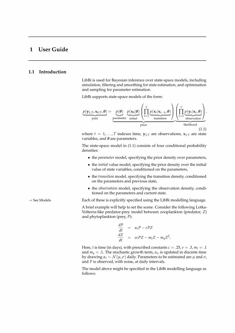
LibBi supports state-space models of the form:

p(y1:T , x0:T , θ)︸ ︷︷ ︸joint

= p(θ)︸︷︷︸parameter

p(x0|θ)︸ ︷︷ ︸initial

T

∏t=1

p(xt|xt−1, θ)︸ ︷︷ ︸transition

︸ ︷︷ ︸

prior

T

∏t=1

p(yt|xt, θ)︸ ︷︷ ︸observation

︸ ︷︷ ︸

likelihood

.

(1.1)where t = 1, . . . , T indexes time, y1:T are observations, x1:T are statevariables, and θ are parameters.

The state-space model in (1.1) consists of four conditional probabilitydensities:

• the parameter model, specifying the prior density over parameters,

• the initial value model, specifying the prior density over the initialvalue of state variables, conditioned on the parameters,

• the transition model, specifying the transition density, conditionedon the parameters and previous state,

• the observation model, specifying the observation density, condi-tioned on the parameters and current state.

Each of these is explicitly specified using the LibBi modelling language.→ See Models

A brief example will help to set the scene. Consider the following Lotka-Volterra-like predator-prey model between zooplankton (predator, Z)and phytoplankton (prey, P):

dPdt

= αtP− cPZ

dZdt

= ecPZ−mlZ−mqZ2.

Here, t is time (in days), with prescribed constants c = .25, e = .3, ml = .1and mq = .1. The stochastic growth term, αt, is updated in discrete timeby drawing αt ∼ N (µ, σ) daily. Parameters to be estimated are µ and σ,and P is observed, with noise, at daily intervals.

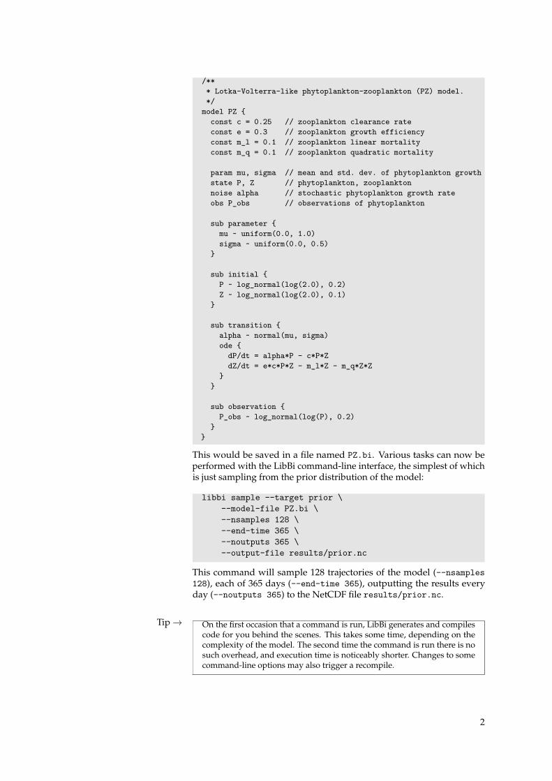
The model above might be specified in the LibBi modelling language asfollows:

/*** Lotka-Volterra-like phytoplankton-zooplankton (PZ) model.*/

model PZ {const c = 0.25 // zooplankton clearance rateconst e = 0.3 // zooplankton growth efficiencyconst m_l = 0.1 // zooplankton linear mortalityconst m_q = 0.1 // zooplankton quadratic mortality

param mu, sigma // mean and std. dev. of phytoplankton growthstate P, Z // phytoplankton, zooplanktonnoise alpha // stochastic phytoplankton growth rateobs P_obs // observations of phytoplankton

sub parameter {mu ~ uniform(0.0, 1.0)sigma ~ uniform(0.0, 0.5)

}

sub initial {P ~ log_normal(log(2.0), 0.2)Z ~ log_normal(log(2.0), 0.1)

}

sub transition {alpha ~ normal(mu, sigma)ode {

dP/dt = alpha*P - c*P*ZdZ/dt = e*c*P*Z - m_l*Z - m_q*Z*Z

}}

sub observation {P_obs ~ log_normal(log(P), 0.2)

}}

This would be saved in a file named PZ.bi. Various tasks can now beperformed with the LibBi command-line interface, the simplest of whichis just sampling from the prior distribution of the model:

libbi sample --target prior \--model-file PZ.bi \--nsamples 128 \--end-time 365 \--noutputs 365 \--output-file results/prior.nc

This command will sample 128 trajectories of the model (--nsamples128), each of 365 days (--end-time 365), outputting the results everyday (--noutputs 365) to the NetCDF file results/prior.nc.

Tip→ On the first occasion that a command is run, LibBi generates and compilescode for you behind the scenes. This takes some time, depending on thecomplexity of the model. The second time the command is run there is nosuch overhead, and execution time is noticeably shorter. Changes to somecommand-line options may also trigger a recompile.

2

To play with this example further, download the PZ package from www.libbi.org. Inspect and run the run.sh script to get started.

The command-line interface provides numerous other functionality, in-cluding filtering and smoothing the model with respect to data, andoptimising or sampling its parameters. The help command is particu-larly useful, and can be used to access the contents of the User Referenceportion of this manual from the command line.

1.2 Getting started

There is a standard file and directory structure for a LibBi project. Usingit for your own projects ensures that they will be easy to share anddistribute as a LibBi package. To set up the standard structure, create anempty directory somewhere, and from within that directory run:

libbi package --create --name Name

replacing Name with the name of your project.

Tip→ By convention, names always begin with an uppercase letter, and all newwords also begin with an uppercase letter, as in CamelCase. See the Styleguide for more such conventions.

Each of the files that are created contains some placeholder content thatis intended to be modified. The META.yml file can be completed imme-diately with the name of the package, the name of its author and a briefdescription. This and other files are detailed with the package command.

This early stage is also the ideal time to think about version control. LibBidevelopers use Git for version control, and you may like to do the samefor your project. A new repository can be initialised in the same directorywith:

git init

Then add all of the initial files to the repository and make the first com-mit:

git add *git commit -m ’Added initial files’

The state of the repository at each commit may be restored at any stage,allowing old versions of files to be maintained without polluting theworking directory.

A complete introduction to Git is beyond the scope of this document.See www.git-scm.com for more information. The documentation for thepackage command also gives some advice on what to include, and whatnot to include, in a version control repository.

The following command can be run at any time to validate that a projectstill conforms to the standard structure:

libbi package --validate

Finally, the following command can be used to build a package for distri-bution:

3

libbi package --build

This creates a *.tar.gz file in the current directory containing the projectfiles.

1.3 Models

Models are specified in the LibBi modelling language. A model specifi-cation is put in a file with an extension of *.bi. Each such file containsonly a single model specification.

A specification always starts with an outer model statement that declaresand names the model. It then proceeds with declarations of constants,dimensions and variables, followed by four top-level blocks – parameter,initial, transition and observation – that describe the factors of thestate-space model.

A suitable template is:

model Name {// declare constants...// declare dimensions...// declare variables...

sub parameter {// specify the parameter model...

}

sub initial {// specify the initial condition model...

}

sub transition {// specify the transition model...

}

sub observation {// specify the observation model...

}}

Note that the contents of the model statement and each top-level block arecontained in curly braces ({. . .}), in typical C-style. Comments are alsoC-style, an inline comment being wrapped by /* and */, and the double-slash (//) denoting an end-of-line comment. Lines may optionally endwith a semicolon.

1.3.1 Constants

Constants are named and immutable scalar values. They are declared→ See also constusing:

const name = constant_expression

Often constant_expression is simply a literal value, but in general itmay be any constant scalar expression (see Expressions).

1.3.2 Inlines

Inlines are named scalar expressions. They are declared using:→ See also inline

4

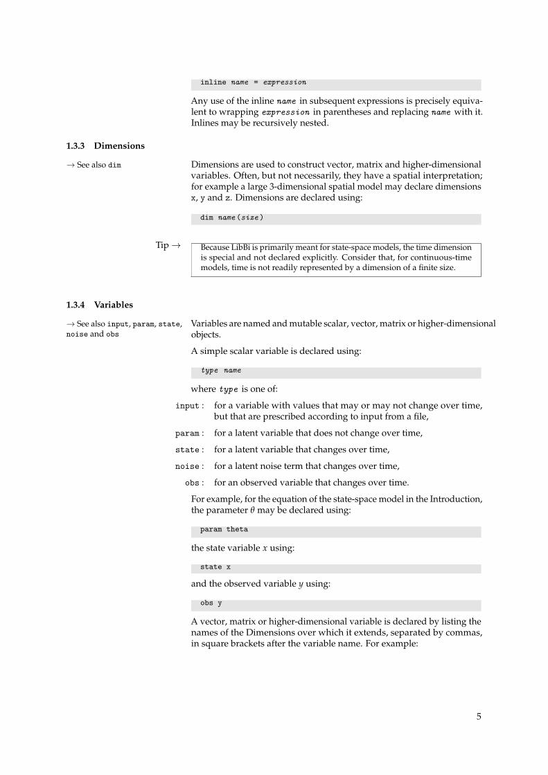
inline name = expression

Any use of the inline name in subsequent expressions is precisely equiva-lent to wrapping expression in parentheses and replacing name with it.Inlines may be recursively nested.

1.3.3 Dimensions

Dimensions are used to construct vector, matrix and higher-dimensional→ See also dimvariables. Often, but not necessarily, they have a spatial interpretation;for example a large 3-dimensional spatial model may declare dimensionsx, y and z. Dimensions are declared using:

dim name (size )

Tip→ Because LibBi is primarily meant for state-space models, the time dimensionis special and not declared explicitly. Consider that, for continuous-timemodels, time is not readily represented by a dimension of a finite size.

1.3.4 Variables

Variables are named and mutable scalar, vector, matrix or higher-dimensional→ See also input, param, state,noise and obs objects.

A simple scalar variable is declared using:

type name

where type is one of:

input : for a variable with values that may or may not change over time,but that are prescribed according to input from a file,

param : for a latent variable that does not change over time,

state : for a latent variable that changes over time,

noise : for a latent noise term that changes over time,

obs : for an observed variable that changes over time.

For example, for the equation of the state-space model in the Introduction,the parameter θ may be declared using:

param theta

the state variable x using:

state x

and the observed variable y using:

obs y

A vector, matrix or higher-dimensional variable is declared by listing thenames of the Dimensions over which it extends, separated by commas,in square brackets after the variable name. For example:

5

dim m(50)dim n(20)...state x[m,n]

declares a state variable x, which is a matrix of size 50× 20.

The declaration of a variable can also include various arguments that con-trol, for example, whether or not it is included in output files. These arespecified in parentheses after the variable declaration, for example:

state x[m,n](has_output = 0)

1.3.5 Actions

Within each top-level block, a probability density is specified using actions.Simple actions take one of three forms:

x ~ expressionx <- expressiondx/dt = expression

where x is some variable, referred to as the target. Named actions, avail-able only for the first two forms, look like:

x ~ name(arguments, ...)x <- name(arguments, ...)

The first form, with the ˜ operator, indicates that the (random) variable xis distributed according to the action given on the right. Such actions areusually named, and correspond to parametric probability distributions(e.g. gaussian, gamma and uniform). If the action is not named, theexpression on the right is assumed to be a probability density function.

The second form, with the <- operator, indicates that the (condition-ally deterministic) variable x should be assigned the result of the actiongiven on the right. Such actions might be simple scalar, vector or matrixexpressions.

The third form, with the = operator, is for expressing ordinary differentialequations.

Individual elements of a vector, matrix or higher-dimensional variablemay be targeted using square brackets. Consider the following actiongiving the ordinary differential equation for a Lorenz ’96 model:

dx[i]/dt = x[i - 1]*(x[i + 1] - x[i - 2]) - x[i] + F

If x is a vector of size N, the action should be interpreted as “for eachi ∈ {0, . . . , N− 1}, use the following ordinary differential equation”. Thename i is an index, considered declared on the left with local scope tothe action, so that it may be used on the right. The name i is arbitrary,but must not match the name of a constant, inline or variable. It maymatch the name of a dimension, and indeed matching the name of thedimension with which the index is associated can be sensible.

Elements of higher-dimensional variables may be targeted using multi-ple indices separated by commas. For example, consider computing aEuclidean distance matrix D:

6

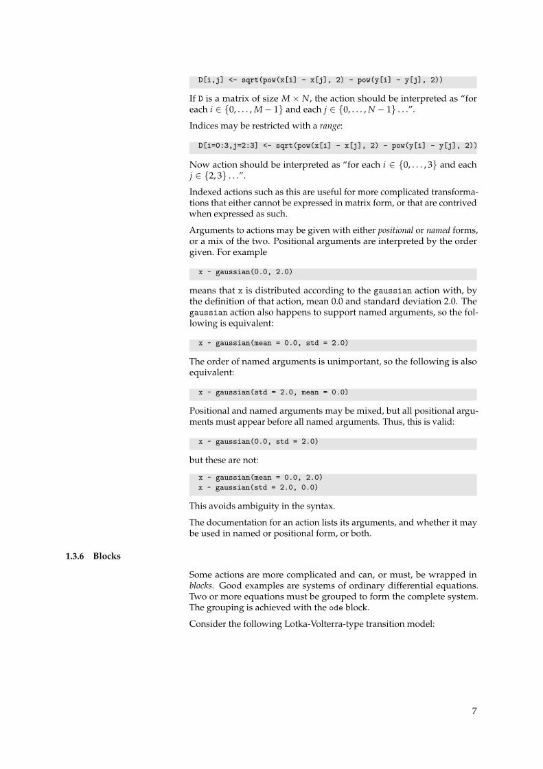
D[i,j] <- sqrt(pow(x[i] - x[j], 2) - pow(y[i] - y[j], 2))

If D is a matrix of size M× N, the action should be interpreted as “foreach i ∈ {0, . . . , M− 1} and each j ∈ {0, . . . , N − 1} . . .”.

Indices may be restricted with a range:

D[i=0:3,j=2:3] <- sqrt(pow(x[i] - x[j], 2) - pow(y[i] - y[j], 2))

Now action should be interpreted as “for each i ∈ {0, . . . , 3} and eachj ∈ {2, 3} . . .”.

Indexed actions such as this are useful for more complicated transforma-tions that either cannot be expressed in matrix form, or that are contrivedwhen expressed as such.

Arguments to actions may be given with either positional or named forms,or a mix of the two. Positional arguments are interpreted by the ordergiven. For example

x ~ gaussian(0.0, 2.0)

means that x is distributed according to the gaussian action with, bythe definition of that action, mean 0.0 and standard deviation 2.0. Thegaussian action also happens to support named arguments, so the fol-lowing is equivalent:

x ~ gaussian(mean = 0.0, std = 2.0)

The order of named arguments is unimportant, so the following is alsoequivalent:

x ~ gaussian(std = 2.0, mean = 0.0)

Positional and named arguments may be mixed, but all positional argu-ments must appear before all named arguments. Thus, this is valid:

x ~ gaussian(0.0, std = 2.0)

but these are not:

x ~ gaussian(mean = 0.0, 2.0)x ~ gaussian(std = 2.0, 0.0)

This avoids ambiguity in the syntax.

The documentation for an action lists its arguments, and whether it maybe used in named or positional form, or both.

1.3.6 Blocks

Some actions are more complicated and can, or must, be wrapped inblocks. Good examples are systems of ordinary differential equations.Two or more equations must be grouped to form the complete system.The grouping is achieved with the ode block.

Consider the following Lotka-Volterra-type transition model:

7

sub transition {sub ode {

dP/dt = alpha*P - c*P*ZdZ/dt = e*c*P*Z - m_l*Z

}}

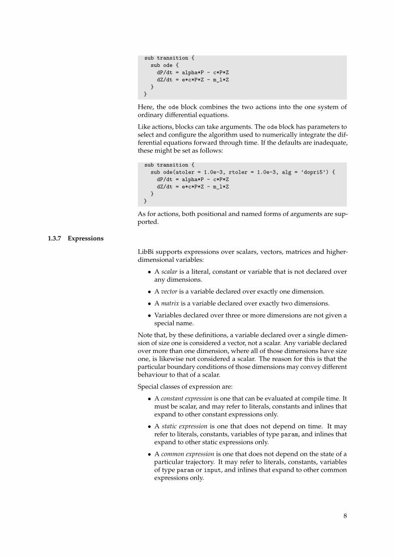
Here, the ode block combines the two actions into the one system ofordinary differential equations.

Like actions, blocks can take arguments. The ode block has parameters toselect and configure the algorithm used to numerically integrate the dif-ferential equations forward through time. If the defaults are inadequate,these might be set as follows:

sub transition {sub ode(atoler = 1.0e-3, rtoler = 1.0e-3, alg = ’dopri5’) {

dP/dt = alpha*P - c*P*ZdZ/dt = e*c*P*Z - m_l*Z

}}

As for actions, both positional and named forms of arguments are sup-ported.

1.3.7 Expressions

LibBi supports expressions over scalars, vectors, matrices and higher-dimensional variables:

• A scalar is a literal, constant or variable that is not declared overany dimensions.

• A vector is a variable declared over exactly one dimension.

• A matrix is a variable declared over exactly two dimensions.

• Variables declared over three or more dimensions are not given aspecial name.

Note that, by these definitions, a variable declared over a single dimen-sion of size one is considered a vector, not a scalar. Any variable declaredover more than one dimension, where all of those dimensions have sizeone, is likewise not considered a scalar. The reason for this is that theparticular boundary conditions of those dimensions may convey differentbehaviour to that of a scalar.

Special classes of expression are:

• A constant expression is one that can be evaluated at compile time. Itmust be scalar, and may refer to literals, constants and inlines thatexpand to other constant expressions only.

• A static expression is one that does not depend on time. It mayrefer to literals, constants, variables of type param, and inlines thatexpand to other static expressions only.

• A common expression is one that does not depend on the state of aparticular trajectory. It may refer to literals, constants, variablesof type param or input, and inlines that expand to other commonexpressions only.

8

Note from these definitions that a constant expression is a static expres-sion, and a static expression is a common expression.

Individual elements of multidimensional variables may be indexed withe.g. x[i] or A[i,j]. Ranges may also be referenced by giving the first andlast indices of the range, separated by a colon, e.g. x[0:3] or A[0:3,2:3].

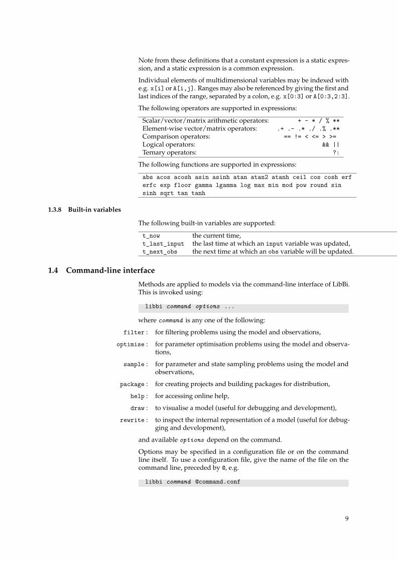
The following operators are supported in expressions:

Scalar/vector/matrix arithmetic operators: + - * / % **Element-wise vector/matrix operators: .+ .- .* ./ .% .**Comparison operators: == != < <= > >=Logical operators: && ||Ternary operators: ?:

The following functions are supported in expressions:

abs acos acosh asin asinh atan atan2 atanh ceil cos cosh erferfc exp floor gamma lgamma log max min mod pow round sinsinh sqrt tan tanh

1.3.8 Built-in variables

The following built-in variables are supported:

t_now the current time,t_last_input the last time at which an input variable was updated,t_next_obs the next time at which an obs variable will be updated.

1.4 Command-line interface

Methods are applied to models via the command-line interface of LibBi.This is invoked using:

libbi command options ...

where command is any one of the following:

filter : for filtering problems using the model and observations,

optimise : for parameter optimisation problems using the model and observa-tions,

sample : for parameter and state sampling problems using the model andobservations,

package : for creating projects and building packages for distribution,

help : for accessing online help,

draw : to visualise a model (useful for debugging and development),

rewrite : to inspect the internal representation of a model (useful for debug-ging and development),

and available options depend on the command.

Options may be specified in a configuration file or on the commandline itself. To use a configuration file, give the name of the file on thecommand line, preceded by @, e.g.

libbi command @command.conf

9

More than one config file may be specified, each preceded by @. Anoption given on the command line will override an option of the samename given in the configuration file.

A config file simply contains a list of command-line options just as theywould be given on the command line itself. For readability, the command-line options may be spread over any number of lines, and end-of-linecomments, preceded by #, may appear. The contents of one config filemay be nested in another by using the @file.conf syntax within a file.This can be useful to avoid redundancy. For example, the sample com-mand inherits all the options of filter. In this case it may be useful towrite a filter.conf file that is nested within a sample.conf file, so thatoptions need not be repeated.

1.5 Output files

LibBi uses NetCDF files for input and output. A NetCDF file consistsof dimensions, along with variables extending across them. This is verysimilar to LibBi models. Where use of these overloaded names may causeconfusion, the specific names NetCDF variable/dimension and model vari-able/dimension are used throughout this section and the next. A NetCDFfile may also contain scalar attributes that provide meta information.

The schema of a NetCDF file is its structure with respect to the dimensions,variables and attributes that it contains. Among the dimensions will bethose that correspond to model dimensions. Likewise for variables. Someadditional dimensions and variables will provide critical method-specificinformation or diagnostics.

Tip→ To quickly inspect the structure and contents of a NetCDF file, use thencdump utility, included as standard in NetCDF distributions:

ncdump file.nc | less

LibBi output files have several schemas. The schema of an output filedepends on the command that produces it, and the options given to thatcommand. The schemas are related by strong conventions and inheritedstructure.

This section outlines each schema in turn. The syntax x[m,n] is usedto refer to a NetCDF variable named x that extends across the NetCDFdimensions named m and n.

Tip→ If using OctBi or RBi for collating and visualising the output of LibBi, it maybe unnecessary to understand these schema, as they are encapsulated bythe higher-level functions of these packages.

1.5.1 Simulation schema

This schema is used by the sample command when the target option isset to prior, joint or prediction. It consists of dimensions:

• nr indexing time,

• np indexing trajectories, and

10

• for each dimension n in the model, a dimension n .

And variables:

• time[nr] giving the output times,

• for each param variable theta in the model, defined over dimen-sions m,...,n , a variable theta [m,...,n ], and

• for each state and noise variable x in the model, defined overdimensions m,...,n , a variable x [nr,m,...,n,np].

1.5.2 Particle filter schema

This schema is used by the filter command when a particle filter, be-sides the adaptive particle filter, is chosen. It extends the simulationschema, with the following changes:

• the np dimension is now interpreted as indexing particles not trajec-tories.

The following variables are added:

• logweight[nr,np] giving the log-weights vector at each time, and

• ancestor[nr,np] giving the ancestry vector at each time.

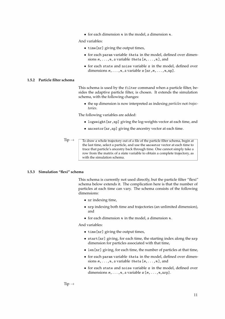
Tip→ To draw a whole trajectory out of a file of the particle filter schema, begin atthe last time, select a particle, and use the ancestor vector at each time totrace that particle’s ancestry back through time. One cannot simply take arow from the matrix of a state variable to obtain a complete trajectory, aswith the simulation schema.

1.5.3 Simulation “flexi” schema

This schema is currently not used directly, but the particle filter “flexi”schema below extends it. The complication here is that the number ofparticles at each time can vary. The schema consists of the followingdimensions:

• nr indexing time,

• nrp indexing both time and trajectories (an unlimited dimension),and

• for each dimension n in the model, a dimension n .

And variables:

• time[nr] giving the output times,

• start[nr] giving, for each time, the starting index along the nrpdimension for particles associated with that time,

• len[nr] giving, for each time, the number of particles at that time,

• for each param variable theta in the model, defined over dimen-sions m,...,n , a variable theta [m,...,n ], and

• for each state and noise variable x in the model, defined overdimensions m,...,n , a variable x [m,...,n,nrp].

Tip→

11

With the “flexi” schema, to read the contents of a variable at some timeindex t , read len[t ] entries along the nrp dimension, beginning at indexstart[t ].

1.5.4 Particle filter “flexi” schema

This schema is used by the filter command when an adaptive particlefilter is chosen. It extends the simulation “flexi” schema. The followingvariables are added:

• logweight[nrp] giving the log-weights vector at each time, and

• ancestor[nrp] giving the ancestry vector at each time.

1.5.5 Kalman filter schema

This schema is used by the filter command when a Kalman filter ischosen. It extends the simulation schema, with the following changes:

• the np dimension is always of size 1, and

• variables that correspond to state and noise variables in the modelare now interpreted as containing the mean of the filter density ateach time.

The following dimensions are added:

• nxcol indexing columns of matrices, and

• nxrow indexing rows of matrices.

The following variables are added:

• U_[nr,nxcol,nxrow] containing the upper-triangular Choleskyfactor of the covariance matrix of the filter density at each time.

• For each noise and state variable x , a variable index.x giving theindex of the first row (and column) in S_ pertaining to this variable,the first such index being zero.

1.5.6 Optimisation schema

This schema is used by the optimise command. It consists of dimensions:

• np indexing iterations of the optimiser (an unlimited dimension).

And variables:

• for each param variable theta in the model, defined over dimen-sions m,...,n , a variable theta [m,...,n,np],

• optimiser.value[np] giving the value of the function being opti-mised at each iteration, and

• optimiser.size[np] giving the value of the convergence criterionat each iteration.

1.5.7 PMCMC schema

This schema is used by the sample command when a PMCMC method ischosen. It extends the simulation schema, with the following changes:

• the np dimension indexes samples, not trajectories, and

12

• for each param variable theta in the model, defined over dimen-sions m,...,n , there is a variable theta [m,...,n,np] instead oftheta [m,...,n ] (i.e. param variables are defined over the np di-mension also).

The following variables are added:

• loglikelihood[np] giving the log-likelihood estimate p̂(y1:T |θp)for each sample θp, and

• logprior[np] giving the log-prior density p(θp) of each sampleθp.

1.5.8 SMC2 schema

This schema is used by the sample command when an SMC2 method ischosen. It extends the PMCMC schema, with the following additionalvariables:

• logweight[np] giving the log-weights vector of parameter sam-ples.

• logevidence[nr] giving the incremental log-evidence of the modelat each time.

1.6 Input files

Input files take three forms:

• initialisation files, containing the initial values of state variables,

• input files, containing the values of input variables, possibly chang-ing across time, and

• observation files, containing the observed values of obs variables.

All of these use the same schema. That schema is quite flexible, allowingfor the representation of both dense and sparse input. Sparsity may bein time or space. Sparsity in time is, for example, having a discrete-timemodel with a scalar obs variable that is not necessary observed at alltimes. Sparsity in space is, for example, having a discrete-time modelwith a vector obs variable, for which not all of the elements are necessarilyobserved at all times.

Each model variable is associated with a NetCDF variable of the samename. Additional NetCDF variables may exist. Model variables whichcannot be matched to a NetCDF variable of the same name do not receiveinput from the file. For input variables, this means that they will remainuninitialised. For spatially dense input, each such NetCDF variable maybe defined along the following dimensions, in the order given:

1. Optionally, a dimension named ns, used to index multiple exper-iments set up in the same file. If not given for a variable, thatvariable is assumed to be the same for all experiments.

2. Optionally, a time dimension (see below).

3. Optionally, a number of dimensions with names that match themodel dimensions along which the model variable is defined, or-dered accordingly,

13

4. Optionally, a dimension named np, used to index multiple trajec-tories (instantiations, samples, particles) of a variable. If not givenfor a variable, the value of that variable is assumed to be the samefor all trajectories. Variables of type param, input and obs may notuse an np dimension, as by their nature they are meant to be incommon across all trajectories.

For spatially sparse input, see Coordinate variables below.

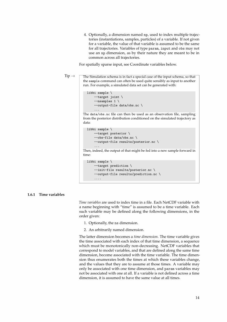
Tip→ The Simulation schema is in fact a special case of the input schema, so thatthe sample command can often be used quite sensibly as input to anotherrun. For example, a simulated data set can be generated with:

libbi sample \--target joint \--nsamples 1 \--output-file data/obs.nc \...

The data/obs.nc file can then be used as an observation file, samplingfrom the posterior distribution conditioned on the simulated trajectory asdata:

libbi sample \--target posterior \--obs-file data/obs.nc \--output-file results/posterior.nc \...

Then, indeed, the output of that might be fed into a new sample forward intime:

libbi sample \--target prediction \--init-file results/posterior.nc \--output-file results/prediction.nc \....

1.6.1 Time variables

Time variables are used to index time in a file. Each NetCDF variable witha name beginning with “time” is assumed to be a time variable. Eachsuch variable may be defined along the following dimensions, in theorder given:

1. Optionally, the ns dimension.

2. An arbitrarily named dimension.

The latter dimension becomes a time dimension. The time variable givesthe time associated with each index of that time dimension, a sequencewhich must be monotonically non-decreasing. NetCDF variables thatcorrespond to model variables, and that are defined along the same timedimension, become associated with the time variable. The time dimen-sion thus enumerates both the times at which these variables change,and the values that they are to assume at those times. A variable mayonly be associated with one time dimension, and param variables maynot be associated with one at all. If a variable is not defined across a timedimension, it is assumed to have the same value at all times.

14

Time variables and time dimensions are interpreted slightly differentlyfor each of the input file types:

1. For an initialisation file, the starting time (given by the --start-timecommand-line option, see filter) is looked-up in each time vari-able, and the corresponding record in each associated variable isused for its initialisation.

2. For input files, a time variable gives the times at which each asso-ciated variable changes in value. Each variable maintains its newvalue until the time of the next change.

3. For observation files, a time variable gives the times at which eachassociated variable is observed. The value of each variable is inter-preted as being its value at that precise instant in time.

Example→ Representing a scalar inputAssume that we have an obs variable named y, and we wish to construct anobservation file containing our data set, which consists of observations of yat various times. A valid NetCDF schema would be:

• a dimension named nr, to be our time dimension,

• a variable named time_y, defined along the dimension nr, to be ourtime variable, and

• a variable named y, defined along the dimension nr, to contain theobservations.

We would then fill the variable time_y with the observation times of ourdata set, and y with the actual observations. It may look something like this:

time_y[nr] y[nr]0.0 6.751.0 4.562.0 9.455.5 4.236.0 7.129.5 5.23

Example→

15

Representing a vector input, denselyAssume that we have an obs variable named y, which is a vector definedacross a dimension of size three called n. We wish to construct an obser-vation file containing a our data set, which consists of observations of y atvarious times, where at each time all three elements of y are observed. Avalid NetCDF schema would be:

• a dimension named nr, to be our time dimension,

• a variable named time_y, defined along the dimension nr, to be ourtime variable,

• a dimension named n, and

• a variable named y, defined along the dimensions nr and n, to containthe observations.

We would then fill the variable time_y with the observation times of ourdata set, and y with the actual observations. It may look something like this:

time_y[nr] y[nr,n]0.0 6.75 3.34 3.451.0 4.56 4.54 1.342.0 9.45 3.43 1.655.5 4.23 8.65 4.646.0 7.12 4.56 3.539.5 5.23 3.45 3.24

1.6.2 Coordinate variables

Coordinate variables are used for spatially sparse input. Each variable witha name beginning with “coord” is assumed to be a coordinate variable.Each such variable may be defined along the following dimensions, inthe order given:

1. Optionally, the ns dimension.

2. A coordinate dimension (see below).

3. Optionally, some arbitrary dimension.

The second dimension, the coordinate dimension, may be a time dimensionas well. NetCDF variables that correspond to model variables, and thatare defined along the same coordinate dimension, become associatedwith the coordinate variable. The coordinate variable is used to indicatewhich elements of these variables are active. The last dimension, ifany, should have a length equal to the number of dimensions acrosswhich these variables are defined. So, for example, if these variables arematrices, the last dimension should have a length of two. If the variablesare vectors, so that they have only one dimension, the coordinate variableneed not have this last dimension.

If a variable specified across one or more dimensions in the model can-not be associated with a coordinate variable, then it is assumed to berepresented densely.

Example→

16

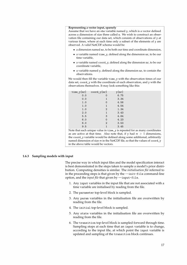
Representing a vector input, sparselyAssume that we have an obs variable named y, which is a vector definedacross a dimension of size three called n. We wish to construct an obser-vation file containing our data set, which consists of observations of y atvarious times, where at each time only a subset of the elements of y areobserved. A valid NetCDF schema would be:

• a dimension named nr, to be both our time and coordinate dimension,

• a variable named time_y, defined along the dimension nr, to be ourtime variable,

• a variable named coord_y, defined along the dimension nr, to be ourcoordinate variable,

• a variable named y, defined along the dimension nr, to contain theobservations.

We would then fill the variable time_y with the observation times of ourdata set, coord_y with the coordinate of each observation, and y with theobservations themselves. It may look something like this:

time_y[nr] coord_y[nr] y[nr]0.0 0 6.750.0 1 3.341.0 0 4.561.0 1 4.541.0 2 1.342.0 1 3.435.5 3 4.646.0 0 4.236.0 2 3.539.5 1 3.45

Note that each unique value in time_y is repeated for as many coordinatesas are active at that time. Also note that, if y had m > 1 dimensions,the coord_y variable would be defined along some additional, arbitrarilynamed dimension of size m in the NetCDF file, so that the values of coord_yin the above table would be vectors.

1.6.3 Sampling models with input

The precise way in which input files and the model specification interactis best demonstrated in the steps taken to sample a model’s prior distri-bution. Computing densities is similar. The initialisation file referred toin the proceeding steps is that given by the --init-file command-lineoption, and the input file that given by --input-file.

1. Any input variables in the input file that are not associated with atime variable are initialised by reading from the file.

2. The parameter top-level block is sampled.

3. Any param variables in the initialisation file are overwritten byreading from the file.

4. The initial top-level block is sampled.

5. Any state variables in the initialisation file are overwritten byreading from the file.

6. The transition top-level block is sampled forward through time.Sampling stops at each time that an input variable is to change,according to the input file, at which point the input variable isupdated and sampling of the transition block continues.

17

Note two important points in this procedure:

• An input variable in the input file that is not associated with atime variable is initialised before anything else, whereas an inputvariable that is associated with a time variable is not initialised untilsimulation begins, even if the first entry of that variable indicatesan update at time zero. This has implications as to which inputvariables are, or are not, initialised at the time that the parameterblock is sampled.

• While the parameter and initial blocks are always sampled, thesamples may be later overwritten from the initialisation file. Thus,the initialisation file need not contain a complete set of variables,although behaviour is more intuitive if it does. This behaviour alsoensures pseudorandom reproducibility regardless of the presence,or content, of the initialisation file.

1.7 Getting it all working

This section contains some general advice on the statistical methods em-ployed by LibBi and the tuning that might be required to make the most ofthem. It concentrates on the particle marginal Metropolis-Hastings (PMMH)sampler, used by default by the sample command when sampling fromthe posterior distribution.

PMMH is of the family of particle Markov chain Monte Carlo (PMCMC)methods (Andrieu et al., 2010), which in turn belong to the family ofMarkov chain Monte Carlo (MCMC). A complete introduction to PMMHis beyond the scope of this manual. Murray (2013) provides an introduc-tion of the method and its implementation in LibBi.

When using MCMC methods it is common to perform some short pilotruns to tune the parameters of the method in order to improve its effi-ciency, before performing a final run. In PMMH, the parameters to betuned are the proposal distribution, and the number of particles in theparticle filter, or sequential Monte Carlo (Doucet et al., 2001), componentof the method.

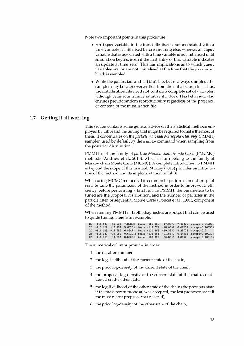
When running PMMH in LibBi, diagnostics are output that can be usedto guide tuning. Here is an example:

22: -116.129 -16.984 7.25272 beats -121.853 -17.6397 7.49326 accept=0.21739123: -116.129 -16.984 5.63203 beats -119.772 -18.0891 6.07209 accept=0.20833324: -116.129 -16.984 6.89478 beats -121.268 -19.3354 8.25723 accept=0.225: -116.129 -16.984 0.643236 beats -136.661 -21.5339 6.44331 accept=0.19230826: -116.129 -16.984 3.58096 beats -128.692 -20.3304 6.3502 accept=0.185185

The numerical columns provide, in order:

1. the iteration number,

2. the log-likelihood of the current state of the chain,

3. the prior log-density of the current state of the chain,

4. the proposal log-density of the current state of the chain, condi-tioned on the other state,

5. the log-likelihood of the other state of the chain (the previous stateif the most recent proposal was accepted, the last proposed state ifthe most recent proposal was rejected),

6. the prior log-density of the other state of the chain,

18

7. the proposal log-density of the other state of the chain, conditionedon the current state, and

8. the acceptance rate of the chain so far.

The last of these is the most important for tuning.

For a standard Metropolis-Hastings, a reasonable guide is to aim at anacceptance rate of 0.5 for a single parameter, down to 0.23 for five ormore parameters (Gelman et al., 1994). This includes the case wherea Kalman filter is being used rather than a particle filter (by using the--filter kalman option to sample). In such cases the only tuning toperform is that of the proposal distribution. The proposal distributionis given in the proposal_parameter block of the model specification. Ifthis block is not specified, the parameter block is used instead, and thismay make for a poor proposal distribution, especially when there aremany observations. Increasing the width of the proposal distributionwill decrease the acceptance rate. Decreasing the width of the proposaldistribution will increase the acceptance rate.

Tip→ Higher acceptance rates are not necessarily better. They may simply be aresult of the chain exploring the posterior distribution very slowly.

PMMH has the added complication of using a particle filter to estimatethe likelihood, rather than a Kalman filter to compute it exactly (althoughnote that the Kalman filter works only for linear and Gaussian models). Itis necessary to set the number of particles in the particle filter. More parti-cles decreases the variance in the likelihood estimator and so increases theacceptance rate, but also increases the computational cost. Because thelikelihood is estimated and not computed exactly, the optimal acceptancerate will be lower than for standard Metropolis-Hastings. Anecdotally,0.1–0.15 seems reasonable.

The tradeoff between proposal size and number of particles is still understudy, e.g. Doucet et al. (2013). The following procedure is suggested.

1. Start with an empty proposal_parameter block. Set the simula-tion time (--end-time) to the time of the first observation, and thenumber of particles (--nparticles) to a modest amount. Whenrunning PMMH, it is then the case that the same state of the chain,its starting state in fact, will be proposed repeatedly, and the accep-tance rate will depend entirely on the variance of the likelihoodestimator. One hopes to see a high acceptance rate here, say 0.5 ormore. Increase the number of particles until this is achieved. Notethat the random number seed can be fixed (--seed) if you wish.

2. Steadily extend the simulation time to include a few more obser-vations on each attempt, and increase the number of particles asneeded to maintain the high acceptance rate. The number of parti-cles will typically need to scale linearly with the simulation time.Consult the Performance guide to improve execution times andfurther increase the number of particles if necessary.

3. If a suitable configuration is achieved for the full data set, or aworkable subset, the proposal distribution can be considered. Youmay find it useful to add one parameter at a time to the proposaldistribution, working towards an overall acceptance rate of 0.1–0.15.

19

4. If this fails to find a working combination with a healthy acceptancerate, consider the initialisation of the chain. By default, LibBi simplydraws a sample from the parameter model to initialise the chain. Ifthis is in an area where the variance in the likelihood estimator ishigh, the chain may mix untenably slowly for any sensible numberof particles. It has been observed empirically that the variance in thelikelihood estimator is heteroskedastic, and tends to increase withdistance from the maximum likelihood (Murray et al., 2013). Soinitialising the chain closer to the maximum likelihood may allow itto mix well with a reasonable number of particles. Prior knowledge,optimisation of parameters (perhaps with the optimise command),or exploration of the data set may inform the initialisation. Theinitialisation can be given in the initialisation file (--init-file).

Tip→ It can also be the case that, in steadily extending the simulation time(--end-time), the acceptance rate suddenly drops at a particular time. Thisindicates that the particle filter degenerates at this point. Improving theinitialisation of the chain is the best strategy in this case, although increasingthe number of particles may help in mild cases.

Be aware that LibBi uses methods that are still being actively developed,and applied to larger and more complex models. It may be the case thatyour model or data set exceeds the current capabilities of the software.In such cases the only option is to consider a smaller or simpler model,or a subsample of the available data.

1.8 Performance guide

One of the aims of LibBi is to alleviate the user from performance con-siderations as much as possible. Nevertheless, there is some scope toinfluence performance, particularly by ensuring that appropriate hard-ware resources are used, and by limiting I/O where possible.

1.8.1 Precomputing

LibBi will:

• precompute constant subexpressions, and

• precompute static subexpressions in the transition and observationmodels.

Reducing redundant or repetitious expressions is thus unnecessary wherethese are constant or static. For example, taking the square-root of avariance parameter need not be of concern:

param sigma2. . .sub transition {

epsilon ~ gaussian(mu, sqrt(sigma2)). . .

}

Here, sqrt(sigma2) is a static expression that will be extracted andprecomputed outside of the transition block.

Tip→

20

Use the rewrite command to inspect precisely which expressions havebeen extracted for precomputation.

1.8.2 I/O

The following I/O options are worth considering to reduce the size ofoutput files and so the time spent writing to them:

• When declaring a variable, use a has_output = 0 argument to omitit from output files if it will not be of interest.

• Enable output files by using the --enable-single command-lineoption. This will reduce write size by up to a half. Note, however,that all computations are then performed in single precision too,which may have significant numerical implications.

1.8.3 Configuration

The following configuration options are worth considering:

• Internally, LibBi uses extensive assertion checking to catch pro-gramming and code generation errors. These assertion checks areenabled by default, improving robustness at the expense of perfor-mance. It is recommended that they remain enabled during modeldevelopment and small-scale testing, but that they are disabledfor final production runs. They can be disabled by adding the--disable-assert command-line option.

• Experiment with the --enable-cuda command-line option to makeuse of a CUDA-enabled GPU. This should usually improve perfor-mance, as long as a sufficient number of model trajectories are tobe simulated (typically upwards of 1024). If CUDA is being used,also try the --enable-gpu-cache command-line option if runningPMCMC or SMC2. This caches particle histories in GPU rather thanmain memory. As GPU memory is usually much more limited thanmain memory, and this may result in its exhaustion, the option isdisabled by default.

• Experiment with the --enable-sse and --enable-avx command-line options to make use of CPU SSE and AVX SIMD instructions. Insingle precision, these can provide up to a four-fold (SSE) or eight-fold (AVX) speed-up, and in double precision a two-fold (SSE) orfour-fold (AVX) speed-up. These are only supported on x86 CPUarchitectures, however, and AVX in particular only on the mostrecent of these.

• Experiment with the --nthreads command-line option to set thenumber of CPU threads. Typically there are depreciating gainsas the number of threads is increased, and beyond the number ofphysical CPU cores performance will degrade significantly. ForCPUs with hyperthreading enabled, it is recommended that thenumber of threads is set to no more than the number of physicalCPU cores. This may be half the default number of threads.

• Experiment with using single precision floating point operations byusing the --enable-single command-line option. This can offersignificant performance improvements (especially when used inconjunction with the --enable-cuda and --enable-sse options),but care should be taken to ensure that numerical error remains

21

tolerable. The use of single precision will also reduce memoryconsumption by up to a half.

• Use optimised versions of libraries, especially the BLAS and LA-PACK libraries.

• Use the Intel C++ compiler if available. Anecdotally, this tendsto produce code that runs faster than gcc. The configure scriptshould automatically detect the Intel C++ compiler, and use it ifavailable. To use the Intel Math Kernel Library as well, which isnot automatically detected, use the --enable-mkl command-lineoption.

1.9 Style guide

The following conventions are used for LibBi model files:

• Model names are CamelCase, the first letter always capitalised.

• Action and block names are all lowercase, with multiple wordsseparated by underscores.

• Dimension and variable names should be consistent, where possi-ble, with their counterparts in a description of the model as it mightappear in a scientific paper. For example, single upper-case lettersfor the names of matrix variables are appropriate, and standardsymbols (rather than descriptive names) are encouraged. Greekletters should be written out in full, the first letter capitalised forthe uppercase version (e.g. gamma and Gamma).

• Comments should be used liberally, with descriptions providedfor all dimensions and variables in particular. Consider includingunits as part of the description, where relevant.

• Names ending in an underscore are intended for internal use only.They are not expected to be seen in a model file.

• Indent using two spaces, and do not use tabs.

Finally, use the package command to set up the standard files and di-rectory structure for a LibBi project. This will make your model and itsassociated files easy to distribute, and your results easy to reproduce.

22

2 User Reference

2.1 Models

2.1.1 model

Declare a model.

Synopsismodel Name {

. . .}

Description

A model statement declares and names a model, and encloses declarationsof the constants, dimensions, variables, inlines and top-level blocks thatspecify that model.

The following named top-level blocks are supported, and should usuallybe provided:

• parameter, specifying the prior density over parameters,

• initial, specifying the prior density over initial conditions,

• transition, specifying the transition density, and

• observation, specifying the observation density.

The following named top-level blocks are supported, and may optionallybe provided:

• proposal_parameter, specifying a proposal density over parame-ters,

• proposal_initial, specifying a proposal density over initial con-ditions,

• lookahead_transition, specifying a lookahead density to accom-pany the transition density, and

• lookahead_observation, specifying a lookahead density to accom-pany the observation density.

2.1.2 dim

Declare a dimension.

Synopsisdim name(100, ’cyclic’)dim name(size = 100, boundary = ’cyclic’)

Description

A dim statement declares a dimension with a given size and boundarycondition.

A dimension may be declared anywhere in a model specification. Itsscope is restricted to the block in which it is declared. A dimension mustbe declared before any variables that extend along it are declared.

Arguments

size : (position 0, mandatory)

Length of the dimension.

boundary : (position 1, default ’none’)

Boundary condition of the dimension. Valid values are:

’none’ : No boundary condition.

’cyclic’ : Cyclic boundary condition; all indexing is taken modulo thesize of the dimension.

’extended’ : Extended boundary condition; indexes outside the range of thedimension access the edge elements, as if these are extendedindefinitely.

2.1.3 input, noise, obs, param and state

Declare an input, noise, observed, parameter or state variable.

Synopsisstate x // scalar variablestate x[i] // vector variablestate X[i,j] // matrix variablestate X[i,j,k] // higher-dimensional variablestate X[i,j](has_output = 0) // omit from output filesstate x, y, z // multiple variables

Description

Declares a variable of the given type, extending along the dimensionslisted between the square brackets.

A variable may be declared anywhere in a model specification. Its scopeis restricted to the block in which it is declared. Dimensions along which avariable extends must be declared prior to the declaration of the variable,using the dim statement.

Arguments

has_input : (default 1)

Include variable when doing input from a file?

has_output : (default 1)

Include variable when doing output to a file?

input_name : (default the same as the name of the variable)

Name to use for the variable in input files.

24

output_name : (default the same as the name of the variable)

Name to use for the variable in output files.

2.1.4 const

Declare a constant.

Synopsisconst name = constant_expression

Description

A const statement declares a constant, the value of which is evaluatedusing the given constant expression. The constant may then be used, byname, in other expressions.

A constant may be declared anywhere in a model specification. Its scopeis restricted to the block in which it is declared.

2.1.5 inline

Declare an inline.

Synopsisinline name = expression...x <- 2*name // equivalent to x <- 2*(expression)

Description

An inline statement declares an inline, the value of which is an expres-sion that will be substituted in place of any occurrence of the inline’sname in other expressions. The inline may be used in any expressionwhere it will not violate the constraints on that expression (e.g. an in-line expression that refers to a state variable may not be used within aconstant expression).

An inline expression may be declared anywhere in a model specification.Its scope is restricted to the block in which it is declared.

2.2 Actions

2.2.1 beta

Beta distribution.

Synopsisx ~ beta()x ~ beta(1.0, 1.0)x ~ beta(alpha = 1.0, beta = 1.0)

Description

A beta action specifies that a variable is beta distributed according to thegiven alpha and beta parameters.

25

Parameters

alpha : (position 0, default 1.0)

First shape parameter of the distribution.

beta : (position 1, default 1.0)

Second shape parameter of the distribution.

2.2.2 betabin

Beta-binomial distribution.

Synopsisx ~ betabin()x ~ betabin(10, 1.0, 2.0)x ~ betabin(n=10, alpha = 1.0, beta = 2.0)

Description

A betabin action specifies that a variable is distributed according to aBeta-binomial distribution with the given number of trials n, and alphaand beta parameters. Note that the implementation will evaluate den-sities for any (not necessarily integer) x. It is left to the user to ensureconsistency (e.g., using this only with integer observations).

Parameters

n : (position 0, default 1)

Number of trials

alpha : (position 1, default 1.0)

First shape parameter of the distribution.

beta : (position 2, default 1.0)

Second shape parameter of the distribution.

2.2.3 binomial

Binomial distribution.

Synopsisx ~ binomial()x ~ binomial(1, 0.5)x ~ binomial(size = 1, prob = 0.5)

Description

A binomial action specifies that a variable is distributed according to abinomial distribution with the given size and prob parameters. Notethat the implementation will evaluate densities for any (not necessarilyinteger) x. It is left to the user to ensure consistency (e.g., using this onlywith integer observations).

26

Parameters

size : (position 0, default 1)

Mean parameter of the distribution.

prob : (position 1, default 0.5)

Shape parameter of the distribution.

2.2.4 cholesky

Cholesky factorisation.

SynopsisU <- cholesky(A)L <- cholesky(A, ’L’)

Description

A cholesky action performs a Cholesky factorisation of a symmetric,positive definite matrix, returning either the lower- or upper-triangularfactor, with the remainder of the matrix set to zero.

Parameters

A : (position 0, mandatory)

The symmetric, positive definite matrix to factorise.

uplo : (position 1, default ’U’)

’U’ for the upper-triangular factor, ’L’ for the lower-triangularfactor. As A must be symmetric, this also indicates which triangleof A is read; other elements are ignored.

2.2.5 exclusive_scan

Exclusive scan primitive (also called prefix sum or cumulative sum).

SynopsisX <- exclusive_scan(x)

Description

An exclusive_scan action computes into each element i of X, the sumof the first i - 1 elements of x.

Parameters

x : (position 0, mandatory)

The vector over which to scan.

2.2.6 exponential

Exponential distribution.

Synopsis

27

x ~ exponential()x ~ exponential(1)x ~ exponential(lambda = 1)

Description

A exponential action specifies that a variable is distributed according toan exponential distribution with the given rate lambda

Parameters

lambda : (position 0, default 1)

Rate

2.2.7 gamma

Gamma distribution.

Synopsisx ~ gamma()x ~ gamma(2.0, 5.0)x ~ gamma(shape = 2.0, scale = 5.0)

Description

A gamma action specifies that a variable is gamma distributed accordingto the given shape and scale parameters.

Parameters

shape : (position 0, default 1.0)

Shape parameter of the distribution.

scale : (position 1, default 1.0)

Scale parameter of the distribution.

2.2.8 gaussian

Gaussian distribution.

Synopsisx ~ gaussian()x ~ gaussian(0.0, 1.0)x ~ gaussian(mean = 0.0, std = 1.0)

Description

A gaussian action specifies that a variable is Gaussian distributed ac-cording to the given mean and std parameters.

Parameters

mean : (position 0, default 0.0)

Mean.

std : (position 1, default 1.0)

Standard deviation.

28

2.2.9 inclusive_scan

Inclusive scan primitive (also called prefix sum or cumulative sum).

SynopsisX <- inclusive_scan(x)

Description

An inclusive_scan action computes into each element i of X, the sumof the first i elements of x.

Parameters

x : (position 0, mandatory)

The vector over which to scan.

2.2.10 inverse_gamma

Inverse gamma distribution.

Synopsisx ~ inverse_gamma()x ~ inverse_gamma(2.0, 1.0/5.0)x ~ inverse_gamma(shape = 2.0, scale = 1.0/5.0)

Description

An inverse_gamma action specifies that a variable is inverse-gammadistributed according to the given shape and scale parameters.

Parameters

shape : (position 0, default 1.0)

Shape parameter of the distribution.

scale : (position 1, default 1.0)

Scale parameter of the distribution.

2.2.11 log_gaussian

Log-Gaussian distribution.

Synopsisx ~ log_gaussian()x ~ log_gaussian(0.0, 1.0)x ~ log_gaussian(mean = 0.0, std = 1.0)

Description

A log_gaussian action specifies that the logarithm of a variable is Gaus-sian distributed according to the given mean and std parameters.

29

Parameters

mean : (position 0, default 0.0)

Mean of the log-transformed variable.

std : (position 1, default 1.0)

Standard deviation of the log-transformed variable.

2.2.12 log_normal

Log-normal distribution, synonym of log_gaussian.

→ See also log_gaussian

2.2.13 negbin

Negative binomial distribution.

Synopsisx ~ negbin()x ~ negbin(1.0, 2.0)x ~ negbin(mean = 1.0, shape = 2.0)

Description

A negbin action specifies that a variable is distributed according to a neg-ative binomial distribution with the given mean and shape parameters(yielding variance mean + meanˆ2/shape). Note that the implementationwill evaluate densities for any (not necessarily integer) x. It is left to theuser to ensure consistency (e.g., using this only with integer observa-tions).

Parameters

mean : (position 0, default 1.0)

Mean parameter of the distribution.

shape : (position 1, default 1.0)

Shape parameter of the distribution.

2.2.14 normal

Normal distribution, synonym of gaussian.

→ See also gaussian

2.2.15 pdf

Arbitrary probability density function.

Synopsisx ~ expressionx ~ pdf(pdf = expression, max_pdf = expression)x ~ pdf(pdf = log_expression, log = 1)

30

Description

A pdf action specifies that a variable is distributed according to somearbitrary probability density function. It need not be used explicitlyunless a maximum probability density function needs to be suppliedwith it: any expression using the ˜ operator without naming an action isevaluated using pdf.

Parameters

pdf : (position 0)

An expression giving the probability density function.

max_pdf : (position 1, default inf)

An expression giving the maximum of the probability density func-tion.

log : (default 0)

Is the expression given the log probability density function?

2.2.16 poisson

Poisson distribution.

Synopsisx ~ poisson()x ~ poisson(1.0)x ~ poisson(rate = 2.0)

Description

A poisson action specifies that a variable is Poisson distributed accordingto the given rate parameter. Note that the implementation will evaluatedensities for any (not necessarily integer) x. It is left to the user to ensureconsistency (e.g., using this only with integer observations).

Parameters

rate : (position 0, default 1.0)

Rate parameter of the distribution.

2.2.17 transpose

Transpose a matrix.

SynopsisB <- transpose(A)

Description

A transpose action performs a matrix transpose.

Parameters

A : (position 0, mandatory)

The matrix.

31

2.2.18 truncated_gaussian

Truncated Gaussian distribution.

Synopsisx ~ truncated_gaussian(0.0, 1.0, -2.0, 2.0)x ~ truncated_gaussian(0.0, 1.0, lower = -2.0, upper = 2.0)x ~ truncated_gaussian(0.0, 1.0, upper = 2.0)

Description

A truncated_gaussian action specifies that a variable is distributedaccording to a Gaussian distribution with a closed lower and/or upperbound.

For a one-sided truncation, simply omit the relevant lower or upperargument.

The current implementation uses a naive rejection sampling with the fullGaussian distribution used as a proposal. The rejection rate is simplythe area under the Gaussian curve between lower and upper. If this issignificantly less than one, the rejection rate will be high, and performanceslow.

Parameters

mean : (position 0, default 0.0)

Mean.

std : (position 1, default 1.0)

Standard deviation.

lower : (position 2)

Lower bound.

upper : (position 3)

Upper bound.

2.2.19 truncated_normal

Truncated normal distribution, synonym of truncated_gaussian.

→ See alsotruncated_gaussian

2.2.20 uniform

Uniform distribution.

Synopsisx ~ uniform()x ~ uniform(0.0, 1.0)x ~ uniform(lower = 0.0, upper = 1.0)

Description

A uniform action specifies that a variable is uniformly distributed on afinite and left-closed interval given by the bounds lower and upper.

32

Parameters

lower : (position 0, default 0.0)

Lower bound on the interval.

upper : (position 1, default 1.0)

Upper bound on the interval.

2.2.21 wiener

Wiener process.

SynopsisdW ~ wiener()

Description

A wiener action specifies that a variable is an increment of a Wienerprocess: Gaussian distributed with mean zero and variance tj - ti,where ti is the starting time, and tj the ending time, of the current timeinterval

2.3 Blocks

2.3.1 bridge

The bridge potential.

Synopsissub bridge {

. . .}

Description

Actions in the bridge block may reference variables of any type, butmay only target variables of type noise and state. References to obsvariables provide their next value. Use of the built-in variables t_nowand t_next_obs will be useful.

2.3.2 initial

The prior distribution over the initial values of state variables.

Synopsissub initial {

. . .}

Description

Actions in the initial block may only refer to variables of type param,input and state. They may only target variables of type state.

2.3.3 lookahead_observation

A likelihood function for lookahead operations.

33

Synopsissub lookahead_observation {

. . .}

Description

This may be a deterministic, computationally cheaper or perhaps inflatedversion of the likelihood function. It is used by the auxiliary particle filter.

Actions in the lookahead_observation block may only refer to variablesof type param, input and state. They may only target variables of typeobs.

2.3.4 lookahead_transition

A transition distribution for lookahead operations.

Synopsissub lookahead_transition {

. . .}

Description

This may be a deterministic, computationally cheaper or perhaps inflatedversion of the transition distribution. It is used by the auxiliary particlefilter.

Actions in the lookahead_transition block may reference variables ofany type except obs, but may only target variables of type noise andstate.

2.3.5 observation

The likelihood function.

Synopsissub observation {

. . .}

Description

Actions in the observation block may only refer to variables of typeparam, input and state. They may only target variables of type obs.

2.3.6 ode

System of ordinary differential equations.

Synopsisode(alg = ’RK4(3)’, h = 1.0, atoler = 1.0e-3, rtoler = 1.0e-3) {

dx/dt = . . .dy/dt = . . .. . .

}

34

ode(’RK4(3)’, 1.0, 1.0e-3, 1.0e-3) {dx/dt = . . .dy/dt = . . .. . .

}

Description

An ode block is used to group multiple ordinary differential equationsinto one system, and configure the numerical integrator used to simulatethem.

An ode block may not contain nested blocks, and may only containordinary differential equation actions.

Parameters

alg : (position 0, default ’RK4(3)’)

The numerical integrator to use. Valid values are:

’RK4’ : The classic order 4 Runge-Kutta with fixed step size.

’RK5(4)’ : An order 5(4) Dormand-Prince with adaptive step size.

’RK4(3)’ : An order 4(3) low-storage Runge-Kutta with adaptive stepsize.

h : (position 1, default 1.0)

For a fixed step size, the step size to use. For an adaptive step size,the suggested initial step size to use.

atoler : (position 2, default 1.0e-3)

The absolute error tolerance for adaptive step size control.

rtoler : (position 3, default 1.0e-3)

The relative error tolerance for adaptive step size control.

2.3.7 parameter

The prior distribution over parameters.

Synopsissub parameter {

. . .}

Description

Actions in the parameter block may only refer to variables of type inputand param. They may only target variables of type param.

2.3.8 proposal_initial

A proposal distribution over the initial values of state variables.

Synopsis

35

sub proposal_initial {x ~ gaussian(x, 1.0) // local proposalx ~ gaussian(0.0, 1.0) // independent proposal

}

Description

This may be a local or independent proposal distribution, used by thesample command when the --with-transform-initial-to-param op-tion is used.

Actions in the proposal_initial block may only refer to variables oftype param, input and state. They may only target variables of typestate.

2.3.9 proposal_parameter

A proposal distribution over parameters.

Synopsissub proposal_parameter {

theta ~ gaussian(theta, 1.0) // local proposaltheta ~ gaussian(0.0, 1.0) // independent proposal

}

Description

This may be a local or independent proposal distribution, used by thesample command.

Actions in the proposal_parameter block may only refer to variables oftype input and param. They may only target variables of type param.

2.3.10 transition

The transition distribution.

Synopsissub transition(delta = 1.0) {

. . .}

Description

Actions in the transition block may reference variables of any typeexcept obs, but may only target variables of type noise and state.

Parameters

delta : (position 0, default 1.0)

The time step for discrete-time components of the transition. Mustbe a constant expression.

36

2.4 Commands

2.4.1 Build options

Options that start with --enable- may be negated by instead startingthem with --disable-.

--dry-parse : (default off)

Do not parse model file. Implies --dry-gen.

--dry-gen : (default off)

Do not generate code.

--dry-build : (default off)

Do not build.

--force : (default off)

Force all build steps to be performed, even when determined notto be required.

--enable-warnings : (default off)

Enable compiler warnings.

--enable-assert : (default on)

Enable assertion checking. This is recommended for test runs, butnot for production runs.

--enable-extra-debug : (default off)

Enable extra debugging options in compilation. This is recom-mended along with --with-gdb or --with-cuda-gdb when debug-ging.

--enable-diagnostics n : (default 0)

Enable diagnostic output n to standard error.

--enable-diagnostics2 : (default off)

Enable another type of diagnostic.

--enable-single : (default off)

Use single-precision floating point.

--enable-openmp : (default on)

Use OpenMP multithreading.

--enable-cuda : (default off)

Enable CUDA code for graphics processing units (GPU).

--enable-cuda-fast-math : (default off)

Enable fast-but-inaccurate instead of slow-but-accurate versions offunctions sin and exp in CUDA.

--enable-gpu-cache : (default off)

For particle filters, enable ancestry caching in GPU memory. GPUmemory is typically much more limited than main memory. If suf-ficient GPU memory is available this may give some performanceimprovement.

37

--cuda-arch : (default sm_30)

For particle filters, enable ancestry caching in GPU memory. GPUmemory is typically much more limited than main memory. If suf-ficient GPU memory is available this may give some performanceimprovement.

--enable-sse : (default off)

Enable SSE code.

--enable-avx : (default off)

Enable AVX code.

--enable-mpi : (default off)

Enable MPI code.

--enable-vampir : (default off)

Enable Vampir profiling.

--enable-gperftools : (default off)

Enable gperftools profiling.

2.4.2 Run options

Options that start with --with- may be negated by instead starting themwith --without-.

--dry-run : Do not run.

--seed : (default automatic)

Pseudorandom number generator seed.

--nthreads N : (default 0)

Run with N threads. If zero, the number of threads used is thedefault for OpenMP on the platform.

--with-gdb : (default off)

Run within the gdb debugger.

--with-valgrind : (default off)

Run within valgrind.

--with-cuda-gdb : (default off)

Run within the cuda-gdb debugger.

--with-cuda-memcheck : (default off)

Run within cuda-memcheck.

--gperftools-file : (default automatic)

Output file to use under --enable-gperftools. The default iscommand.prof.

--mpi-np : Number of processes under --enable-mpi, corresponding to the-np option to mpirun.

--mpi-npernode : Number of processes per node under --enable-mpi. Correspondsto the -npernode option to mpirun.

38

--mpi-hostfile : Host file under --enable-mpi, corresponding to the -hostfileoption to mpirun.

--role : (default client)

When a client-server architecture is used under MPI, the role of theprocess; either client or server.

--server-file : (default port_name)

When a client-server architecture is used under MPI, the file con-taining server connection information. A server process will writeto this file, a client process will read from it.

2.4.3 Common options

The options in this section are common across all client programs.

Input/output options

--model-file : File containing the model specification.

--init-file : File from which to initialise parameters and initial conditions.

--input-file : File from which to read inputs.

--obs-file : File from which to read observations.

--output-file : (default automatic)

File to which to write output. The default is results/command.nc.

--init-ns : (default 0)

Index along the ns dimension of --init-file to use.

--init-np : (default -1)

Index along the np dimension of --init-file to use. -1 indicatesthat, rather than initialising all state variables identically, the npdimension is used to initialise them all differently. The size of thenp dimension must be at least the number of samples.

--input-ns : (default 0)

Index along the ns dimension of --input-file to use.

--input-np : (default -1)

Index along the np dimension of --input-file to use. -1 indicatesthat, when state variables are read from the input file, rather thaninitialising all state variables identically, the np dimension is usedto initialise them all differently. The size of the np dimension mustbe at least the number of samples.

--obs-ns : (default 0)

Index along the ns dimension of --obs-file to use.

--obs-np : (default 0)

Index along the np dimension of --obs-file to use.

39

Model transformations

--with-transform-extended : (default automatic)

Transform the model for use with the extended Kalman filter. Thisincludes symbolically deriving Jacobian expressions.

--with-transform-param-to-state : (default automatic)

Treat parameters as state variables. This is useful for joint state andparameter estimation using filters.

--with-transform-obs-to-state : (default automatic)

Treat observed variables as state variables. This is useful for pro-ducing simulated data sets from a model.

--with-transform-initial-to-param : (default off)

Augment the parameters of the model with the initial values ofstate variables. This is useful when sampling from the posteriordistribution. Treating initial values as parameters means that theyare sampled using local Metropolis-Hastings moves rather than byimportance sampling, which may be beneficial if a good importanceproposal cannot be devised.

2.4.4 draw

Draw a model as a directed graph.

Synopsislibbi draw --model-file Model.bi > Model.dotdot -Tpdf -o Model.pdf Model.dot

Description

The draw command takes a model specification and outputs a directedgraph to visualise the model. It is useful for validation and debuggingpurposes. The output is a dot script that can be processed by the dotprogram to create a figure.

2.4.5 filter

Filtering tasks.

Synopsislibbi filter . . .

Options

The filter command permits the following options:

--start-time : (default 0.0)

Start time.

--end-time : (default 0.0)

End time.

40

--noutputs : (default 0)

Number of dense output times. The state is always output at time--end-time and at all observation times in --obs-file. This argu-ment gives the number of additional, equispaced times at which tooutput. With --end-time T and --noutputs K, then for each k in0,...,K-1, the state will be output at time T*k/K.

--with-output-at-obs : (default 1)

Output at observation times in addition to dense output times.

--filter : (default bootstrap)

The type of filter to use; one of:

bootstrap : Bootstrap particle filter,

lookahead : Auxiliary particle filter with lookahead. The lookahead oper-ates by advancing each particle according to the \blockref{lookahead_transition}top-level block, and weighting according to the \blockref{lookahead_observation}top-level block. If the former is not defined, the \blockref{transition}top-level block will be used instead. If the latter is not defined,the \blockref{observation} top-level block will be used instead.

bridge : Particle filter with intermediate bridging weights, as describedin Del Moral & Murray (2014). Bridging weights are assignedaccording to the \blockref{bridge} top-level block.

kalman : Extended Kalman filter. Jacobian terms are determined bysymbolic manipulations. There are some limitations to thesemanipulations at present, so that some models cannot be han-dled. An error message will be given in these cases.

Setting --filter kalman automatically enables the --with-transform-extendedoption.

Particle filter-specific options The following additional options areavailable when --filter gives a particle filter type:

--nparticles : (default 1)

Number of particles to use.

--ess-rel : (default 0.5)

Threshold for effective sample size (ESS) resampling trigger. Par-ticles will only be resampled if ESS is below this proportion of--nparticles. To always resample, use --ess-rel 1. To neverresample, use --ess-rel 0.

--resampler : (default systematic)

The type of resampler to use; one of:

stratified : for a stratified resampler (Kitagawa 1996),

systematic : for a systematic (or ’deterministic stratified’) resampler (Kita-gawa 1996),

multinomial : for a multinomial resampler,

metropolis : for a Metropolis resampler (Murray 2011),

rejection : for a rejection resampler (Murray, Lee & Jacob 2013), or

41

Metropolis resampler-specific options The following additional op-tions are available when --resampler is set to metropolis.

-C : (default 0)

Number of steps to take.

Bridge particle filter-specific options The following additional optionsare available when --filter is set to bridge:

--nbridges : (default 0)

Number of dense bridge times. This argument gives the number ofequispaced times at which to assign bridge weights, and potentiallyresample. With --end-time T and --nbridges K, then for each kin 0,...,K-1, bridge weighting will occur at time T*k/K.

Adaptive particle filter-specific options The following additional op-tions are available when --filter is set to ’adaptive’:

--stopper : (default deterministic)

The stopping criterion to use; one of:

deterministic : for a fixed number of particles,

sumofweights : for a sum of weights,

miness : for a minimum effective sample size (ESS),

stddev : for a minimum standard deviation,

var : for a minimum variance.

--stopper-threshold : (default 128)

Threshold value for stopping criterion.

--stopper-max : (default 32768)

Maximum number of particles at any time, regardless of the stop-ping criterion.

--stopper-block : (default 128)

Number of particles per block.

2.4.6 help

Look up online help for an action, block or command.

Synopsislibbi help name

libbi help name --action

libbi help name --block

libbi help name --command

42

Description

The help command is used to access documentation from the commandline. This documentation is the same as that provided in the user refer-ence.

name gives the name of any action, block or command. The documen-tation for the respective action, block or command is presented. Ambi-guities (e.g. actions and blocks with the same name) are resolved via aprompt, or by using any of the --action, --block or --command options.

Options

The following options are supported:

--action : explicitly search for an action.

--block : explicitly search for a block.

--command : explicitly search for a command.

2.4.7 optimise

Optimisation of the parameters of a model.

Synopsislibbi optimise . . .

libbi optimize . . .

Alternative spellings are supported.

Options

The optimise command inherits all options from \clientref{filter}, andpermits the following additional options:

--target : (default likelihood)

Optimisation target; one of:

likelihood : Maximum likelihood estimation.

posterior : Maximum a posteriori estimation.

--optimiser or --optimizer : (default nm)

The optimisation method to use; one of:

nm : Nelder-Mead simplex method.

Nelder-mead simplex method-specific options

--simplex-size-real : (default 0.1)

Size of initial simplex relative to starting point of each variable.

--stop-size : (default 1.0-e4)

Size-based stopping criterion.

--stop-steps : (default 100)

Maximum number of steps to take.

43

2.4.8 optimize

Optimization of the parameters of a model.

See also

\clientref{optimise}

2.4.9 package

Create and validate projects, build packages for distribution.

Synopsislibbi package --create

libbi package --validate

libbi package --build

libbi package --webify

Description

LibBi prescribes a standard structure for a project’s model, configuration,data and other files, and a standard format for packaging these. Theformer assists with collaboration and reproducible research, the latterwith distribution.

The package command provides facilities for creating a new LibBi projectwith the standard file and directory structure, and bundling such a projectinto a package for distribution.

A standard project A standard project contains the following files:

*.bi : Model files.

init.sh : A shell script that may be run to create any derived files. A commontask is to call libbi sample --target joint ... to simulate adata set for testing purposes.

run.sh : A shell script that may be run to reproduce the results of the project.Common tasks are to call libbi sample --target prior ... tosample from the prior distribution, and libbi sample --targetposterior ... to sample from the posterior distribution. While auser may not necessarily run this script directly, it should at leastgive them an idea of what the project is set up to do, and whatcommands they might expect to work. After the README.md file,this would typically be the second file that a new user looks at.

*.conf : Configuration files. Common files are prior.conf, posterior.conf,filter.conf and optimise.conf, containing command-line op-tions for typical commands.

config.conf : A particular configuration file where, by convention, a user can setany platform-specific build and run options (such as --enable-cudaand --nthreads). Any LibBi commands in the init.sh and run.shscripts should include this configuration file to bring in the user’sown options (e.g. libbi sample @config.conf ...).

44

data/ : Directory containing data files that are passed to LibBi using the--init-file, --input-file and --obs-file command-line op-tions.

results/ : Directory containing results files created from LibBi using the--output-file command-line option.

A standard package The following additional files are used for thepackaging of a project:

MANIFEST : A list of files, one per line, to be included in the package.

LICENSE : The license governing distribution of the package.

META.yml : Meta data of the package. It should be formatted in YAML, givingthe name, author, version and description of the package. See thatproduced by libbi package --create as a guide.

README.md : A description of the package. This would typically be the first filethat a new user looks at. It should be formatted in Markdown.

VERSION.md : The version history of the package. It should be formatted inMarkdown.

Packages should be given a three-figure version number of theform x.y.z, where x is the version number, y the major revisionnumber and z the minor revision number. The version numberwould typically be incremented after an overhaul of the package,the major revision number after the addition of new functionality,and the minor revision number after bug fixes or corrections. Whena number is incremented, those numbers on the right should bereset to zero. The first version number of a working package shouldbe 1.0.0. If a package is incomplete, only partially working orbeing tested, the version number may be zero.

A project may contain any additional files, and these may be listed in theMANIFEST file for distribution. Commonly included are Octave, MATLABor R scripts for collating and plotting results, for example.

A standard package is simply a gzipped TAR archive with a file name ofName -Version.tar.gz. Extracting the archive produces a directory witha name of Name -Version , within which are all of those files listed in theMANIFEST file of the project.

Version control Under version control, all project files with the excep-tion of the following would be included:

• Any files in the results/ directory. These can be large, and at anyrate are derived files that a user should be able to reproduce forthemselves, perhaps with the run.sh script.

• The results/ directory itself. This is always created automaticallywhen used in the --output-file command-line option, and soits inclusion is unnecessary. Moreover, it is common to create aresults symlink to another directory where output files should bewritten, particularly in a cluster environment where various net-work file systems are available. Inclusion of the results/ directoryin a version control system becomes a nuisance in such cases.

These files would also not typically be included in the package MANIFEST.

45

Options

The following options are supported:

--create : Set up the current working directory as a LibBi project. This createsall the standard files for a LibBi package with placeholder contents.It will prompt to overwrite existing files.

--validate : Validate the current working directory as a LibBi project.

--build : Validate the current working directory as a LibBi project and buildthe package. This produces a Model-x.y.z.tar.gz file in the cur-rent working directory for distribution.

--webify : Create a file for publishing the package on a Jekyl website (suchas www.libbi.org). This produces a Model.md file in the currentworking directory.

Package creation-specific options

--name : (default ’Untitled’)

Name of the package.

2.4.10 rewrite

Output internal model representation after applying transformations andoptimisations.

Synopsislibbi rewrite --model-file Model.bi

Description

The rewrite command takes a model specification and outputs a newspecification that shows the internal transformations and optimisationsapplied by LibBi. It is useful for validation and debugging purposes. Thenew specification is written to stdout.

2.4.11 sample

Sample the prior, joint or posterior distribution.

Synopsislibbi sample --target prior . . .

libbi sample --target joint . . .

libbi sample --target posterior . . .

Options

The sample command inherits all options from filter, and permits thefollowing additional options:

--target : (default posterior)

The target distribution to sample; one of:

prior : To sample from the prior distribution.

46

joint : To sample from the joint distribution. This is equivalent to--target prior --with-transform-obs-to-state.

posterior : To sample from the posterior distribution. Use --obs-file toprovide observations.

prediction : To sample forward in time from a given initial state. Use--init-file to set the initial state, and this initial state deter-mines the interpretation of the prediction. For example, the--init-file may be the output file of a previous sampling ofthe posterior distribution, in which case the result is a posteriorprediction.

--sampler : (default mh)

The type of sampler to use for --target posterior; one of:

mh or (deprecated) pmmh : Marginal Metropolis-Hastings (Andrieu, Doucet & Holenstein,2010).

sir or (deprecated) smc2 : Marginal sequential importance resampling (Chopin, Jacob &Papaspiliopoulos, 2013).

sis : Marginal sequential importance sampling (SIS).

For MH, the proposal works according to the \blockref{proposal_parameter}top-level block in the model. If this is not defined, independentdraws are taken from the \blockref{parameter} top-level block in-stead. If --with-transform-initial-to-param is used, the \blockref{proposal_initial}top-level block is used to make Metropolis-Hastings proposals overinitial conditions also. If this is not defined, independent draws aretaken from the \blockref{initial} top-level block instead.

For SIR, the same blocks are used as proposals for rejuvenationsteps, unless one of the adaptation strategies below is enabled.

--nsamples : (default 1)

Number of samples to draw.

SIR-specific options

--nmoves : (default 1)

Number of move steps to perform after each resample.

--tmoves : (default 0.0)

Overall real time, in seconds, to allocate to move steps (Murrayet al. 2016). If positive, --nmoves and --sample-ess-rel are ig-nored. Resampling is performed after each step, and the number ofmoves subsequently made becomes a random variable dependenton --tmoves.

--sample-resampler : (default systematic)

The type of resampler to use on parameter particles, see --resamplerfor options.

--sample-ess-rel : (default 0.5)

Threshold for effective sample size (ESS) resampling trigger. Param-eter particles will only be resampled if ESS is below this proportion

47

of --nsamples. To always resample, use --sample-ess-rel 1. Tonever resample, use --sample-ess-rel 0.

--sample-stopper : (default deterministic)

The stopping criterion to use for parameter samples while adapting,see --stopper for options.

--sample-stopper-threshold : Threshold value for stopping criterion.

--sample-stopper-max : Maximum number of samples at any time, regardless of the stop-ping criterion.

--adapter : (default none)

Adaptation strategy for rejuvenation proposals:

none : No adaptation.

local : Local proposal adaptation.

global : Global proposal adaptation.

--adapter-scale : (default 0.25)

When local proposal adaptation is used, the scaling factor of thelocal proposal standard deviation relative to the global samplestandard deviation.

--adapter-ess-rel : (default 0.25)

Threshold for effective sample size (ESS) adaptation trigger. Adap-tation will only be performed if ESS is above this proportion of--nsamples. To always adapt, use --adapter-ess-rel 1. If adap-tation is not performed, the proposal_parameter top-level blockis used for rejuvenation proposals instead.

48

3 Developer Guide

3.1 Introduction

LibBi consists of two major components:

• A library that provides classes and functions for simulation, fil-tering, smoothing, optimising and sampling state-space models,as well as auxiliary functionality such as memory management,I/O, numerical computing etc. It is written in C++ using a genericprogramming paradigm.

• A code generator that parses the LibBi modelling language, con-structs and optimises an internal model representation, and gener-ates C++ code for compilation against the library. It also includesthe command-line interface through which the user interacts withLibBi. It is written in Perl using an object-oriented paradigm.

Related projects might also be considered components. These includeOctBi for GNU Octave and RBi for R. Both allow the querying, collationand visualisation of results output by LibBi.

Developing LibBi involves adding or modifying functionality in one ormore of these components. A typical exercise is adding block and actiontypes to the code generator to introduce new features, such as supportfor additional probability density functions. This may also involve im-plementing new functionality in the library that these blocks and actionscan use. Another common task is adding a new inference method tothe library, then adding or modifying the code generator to produce theclient code to call it.

3.2 Setting up a development environment

When developing LibBi, it is recommended that you do not install it inthe usual manner as a system-wide Perl module. The recommendedapproach is to work from a local clone of the LibBi Git repository. Thisway modifications take effect immediately without additional installationsteps, and changes are easily committed back to the repository.

3.2.1 Obtaining the source code

LibBi is hosted on GitHub at https://github.com/libbi/LibBi. It is rec-ommended that you sign up for an account on GitHub and fork therepository there into your own account. You can then clone your forkedrepository to your local machine with:

git clone https://github.com/username/LibBi.git

You should immediately add the original LibBi repository upstream:

cd LibBigit remote add upstream https://github.com/libbi/LibBi.git

after which the following command will pull in changes committed tothe main repository by other developers:

git fetch upstream

To contribute your work back to the main LibBi repository, you can usethe Pull Request feature of GitHub.

Similar instructions apply to working with OctBi and RBi, which are heldin separate repositories under https://github.com/libbi.

When running the command libbi, you will want to make sure that youare calling the version in the Git repository that you have just created. Theeasiest way to do this is to add the LibBi/script directory to your $PATHvariable. LibBi will find the other files itself (it uses the base directory ofthe libbi script to determine the location of other files).

3.2.2 Using Eclipse

LibBi is set up to use the Eclipse IDE (http://www.eclipse.org). Froma vanilla install of the Eclipse IDE for C/C++, a number of additionalplugins are supported, and recommended. These are, along with theURLs of their update sites:

• Eclox (Doxygen integration) http://download.gna.org/eclox/update,

• EPIC (Perl integration) http://e-p-i-c.sf.net/updates/testing, and

• Perl Template Toolkit Editor http://perleclipse.com/TTEditor/UpdateSite.

All of these plugins may be installed via the Help > Install New Software...menu item in Eclipse, in each case entering the update site URL givenabove.

The EGit plugin is bundled with all later versions of Eclipse and canbe used to obtain LibBi from GitHub. Use the File > Import... menuitem, then Git > Projects from Git, URI, and enter the URL of your forkedrepository on GitHub. Follow the prompts from there.

A custom code style is available in the eclipse/custom_code_style.xmlfile, and custom code templates in eclipse/custom_code_templates.xml.These can be installed via the Window > Preferences dialog, using theImport... buttons under C/C++ > Code Style > Formatter and C/C++ >Code Style > Code Templates, respectively. With these installed, Ctrl +Shift + F in an editor window automatically applies the prescribed style.

3.3 Building documentation

This user manual can be built, from the base directory of LibBi, using thecommand:

perl MakeDocs.PL

You will need LATEX installed. The manual will be built in PDF format atdocs/pdf/index.pdf. Documentation of all actions, blocks and clients isextracted from their respective Perl modules as part of this process.

The Perl components of LibBi are documented using POD (“Plain OldDocumentation”), as is conventional for Perl modules. The easiest wayto inspect this is on the command line, using, e.g.

50

perldoc lib/Bi/Model.pm

A PDF or HTML build of the Perl module documentation is not yetavailable.

The C++ components of LibBi are documented using Doxygen. HTMLdocumentation can be built by running doxygen in the base directory ofLibBi, then opening the docs/dev/html/index.html file in a browser.

3.4 Building releases

LibBi is packaged as a Perl module. The steps for producing a new releaseare:

1. Update VERSION.md.

2. Update MANIFEST by removing the current file, running perl MakeManifest.PLand inspecting the results. Extraneous files that should not be dis-tributed in a release are eliminated via regular expressions in theMANIFEST.SKIP file.

3. Run perl Makefile.PL followed by make dist.

On GitHub, the last step is eliminated in favour of tagging the repositorywith version numbers and having archives automatically built by theservice.

3.5 Developing the code generator

The code generator component is implemented in Perl using an object-oriented paradigm, with extensive use of the Perl Template Toolkit (TT)for producing C++ source and other files.

3.5.1 Actions and blocks

A user of LibBi is exposed only to those blocks and actions which theyexplicitly write in their model specification file. Developers must beaware that beyond these explicit blocks, additional implicit blocks areinserted according to the actions specified by the user. In particular, eachaction has a preferred parent block type. If the user, in writing their modelspecification, does not explicitly place an action within its preferred blocktype, the action will be implicitly wrapped in it anyway.

For example, take the model specification:

sub transition {x ~ uniform(x - 1.0, x + 1.0)y ~ gaussian(y, 1.0)

}

The uniform and gaussian actions prefer different parent block types.These additional block types will be inserted, to give the equivalent ofthe user having specified:

51

sub transition {sub uniform_ {

x ~ uniform(x - 1.0, x + 1.0)}sub gaussian_ {

y ~ gaussian(y, 1.0)}

}

For the developer, then, actions and blocks are always written in tandem.Note the underscore suffix on uniform_ and gaussian_ is a conventionthat marks these as blocks for internal use only – the user is not intendedto use them explicitly (see the style guide).

It is worth familiarising yourself with this behaviour, and other transfor-mations made to a model, by using the rewrite command.

To add a block:

1. Choose a name for the block.

2. Create a Perl module Bi::Block::name in the file lib/Bi/Block/name.pm.Note that Perl module “CamelCase” naming conventions shouldbe ignored in favour of LibBi block naming conventions here.

3. Create a new TT template share/tt/cpp/block/name.hpp.tt. Whenrendered, the template will be passed a single variable namedblock, which is an object of the class created in the previous step.

As implementation details of the Perl module and template are subject tochange, it is highly recommended that you copy and modify an existing,similar block type, as the basis for your new block type.

To add an action:

1. Choose a name for the action.

2. Create a Perl module Bi::Action::name in the file lib/Bi/Action/name.pm.Note that Perl module “CamelCase” naming conventions shouldbe ignored in favour of LibBi action naming conventions here.

3. If necessary, create a new TT template share/tt/cpp/action/name.hpp.tt.During rendering, the template will be passed a single variablenamed action, which is an object of the class created in the previ-ous step. This template is not required; the template of the contain-ing block may generate all the necessary code.

3.5.2 Clients

To add a client:

1. Consider whether an existing client can be modified or a new clientshould be added. For an existing client, edit the correspondingPerl module lib/Bi/Client/name.pm. For a new client, choosea name and create a new Perl module lib/Bi/Client/name.pm.Again, LibBi client naming conventions should be favoured overPerl module naming conventions.

2. Consider whether an existing template can be modified or a newtemplate should be created. For an existing template, edit the cor-responding template in share/tt/cpp/client/template.cpp.tt.For a new template:

52

(a) Create files share/tt/cpp/client/template.cpp.tt and share/tt/cpp/client/template.cu.tt.Note that the second typically only needs to #include theformer, the *.cu file extension is merely needed for a CUDA-enabled compile.

(b) Modify the Perl module to select this template for use whereappropriate.

(c) Add the template name to the list given at the top of share/tt/build/Makefile.am.ttto ensure that a build fule is generated for it.

3.5.3 Designing an extension

Complex C++ code should form part of the library, rather than beingincluded in TT templates. The C++ code generated by templates shouldtypically be limited to arranging for a few function calls into the library,where most of the implementation is done.

When writing templates for client programs, consider that it is advanta-geous for the user that they can change command-line options withoutthe C++ code changing, so as to avoid a recompile. This can be achievedby writing runtime checks on command-line options in C++ rather thancode generation-time checks in TT templates. This need not be taken tothe extreme, however: clear and simple template code is preferred overconvoluted C++!

3.5.4 Documenting an extension

Reference documentation for actions, blocks and clients is written in thePerl module created for them, in standard Perl POD. Likewise, param-eters for actions and blocks, and command-line options for clients, areenumerated in these. The idea of this is to keep implementation anddocumentation together.

POD documentation in these modules is automatically converted to LATEXand incorporated in the User Reference section of this manual.

3.5.5 Developing the language

The LibBi modelling language is specified in the files share/bi.lex(for the lexer) and share/bi.yp (for the parser). The latter file makesextensive callbacks to the Bi::Parser module. After either of the twofiles are modified, the automatically-generated Parse::Bi module mustbe rebuilt by running perl MakeParser.PL.

3.5.6 Style guide

Further to the style guide for users, the following additional recommen-dations pertain to developers:

• Action, block, client and argument names are all lowercase, withmultiple words separated by ’_’ (the underscore). Uppercase maybe used in exceptional cases where this convention becomes con-trived. A good example is matrix arguments, which might naturallybe named with uppercase letters.

• Actions, blocks and arguments that are not meant to be used explic-itly should be suffixed with a single underscore.

53

3.6 Developing the library

The library component is implemented in C++ using a generic program-ming paradigm. While classes and objects are used extensively, it is notobject-oriented per se. In particular:

• Class inheritance is used for convenience of implementation, notnecessarily to represent “is a” relationships.

• Polymorphism is seldom, if ever, employed.

• Static dispatch is favoured strongly over dynamic dispatch forreasons related to performance. Virtual functions are not used.

3.6.1 Header files

Header files are given two extensions in LibBi:

1. *.hpp headers may be safely included in any C++ (e.g. *.cpp) orCUDA (*.cu) source files,

2. *.cuh headers may only be safely included in CUDA (*.cu) sourcefiles. They include CUDA C extensions.

Note that not all *.hpp headers can be safely included in *.cu files either,due to CUDA compiler limitations, particularly those headers that furtherinclude Boost headers which make extensive use of templates. Effortshave been made to quarantine such incidences from the CUDA compiler,and support is improving, but mileage may vary.

3.6.2 Pseudorandom reproducibility

It is important to maintain reproducibility of results under the samerandom number seed, typically passed using the --seed option on thecommand line. Real time impacts should be considered, such as favour-ing static scheduling over dynamic scheduling for OpenMP thread blocks.Consider the following:

Random rng;

#pragma omp parallel forfor (int i = 0; i < N; ++i) {x = rng.uniform();. . .

}

Random maintains a separate pseudorandom number generator for eachOpenMP thread. If dynamically scheduled, the above loop gives noguarantees as to the number of variates drawn from each generator, sothat reproducibility of results for a given seed is not guaranteed. Staticscheduling should be enforced in this case to ensure reproducibility:

Random rng;

#pragma omp parallel for schedule(static)for (int i = 0; i < N; ++i) {x = rng.uniform();. . .

}

54

Tip→ To avoid this particular case, static scheduling is enabled by default. Youshould not override this with dynamic scheduling in an OpenMP loop.

A more subtle consideration is the conditional generation of variates.Consider the following code, evaluating a Metropolis-Hastings accep-tance criterion:

alpha = (l1*p1*q2)/(l2*p2*q1);if (alpha >= 1.0 || rng.uniform() < alpha) {accept();

} else {reject();

}

Here, rng.uniform() is called only when alpha >= 1.0 (given operatorshort-circuiting). We might prefer, however, that across multiple runswith the same seed, the pseudorandom number generator is always inthe same state for the nth iteration, regardless of the acceptance criteriaacross the preceding iterations. Moving the variate generation outsidethe conditional will fix this:

alpha = (l1*p1*q2)/(l2*p2*q1);u = rng.uniform();if (alpha >= 1.0 || u < alpha) {accept();

} else {reject();

}

3.6.3 Shallow copy, deep assignment

Typically, classes in LibBi follow a “shallow copy, deep assignment” id-iom. The idiom is most apparent in the case of vector and matrix types.A copy of a vector or matrix object is shallow – the new object merelycontains a pointer to the memory buffer underlying the existing object.An assignment of a vector or matrix is deep, however – the contents ofthe memory buffer underlying the existing object is copied into that ofthe new object.

Often the default copy constructor is sufficient to achieve a shallow copy,while an override of the default assignment operator may be necessaryto achieve deep assignment.

Generic copy constructors and assignment operators are also common.These are templated overloads of the default versions which accept, asarguments, objects of some class other than the containing class. When ageneric copy constructor or assignment operator is used, the default copyconstructor or assignment operator should always be overridden also.

3.6.4 Coding conventions

The following names are used for template parameters (where n is aninteger):

• B for the model type,

• Tn for scalar types,

• Vn for vector types,

55

• Mn for matrix types,

• Qn for pdf types,

• S for type lists,

• L for location (host or device),

• CL for location of a cache,

• PX for parents type,

• CX for coordinates type,

• OX for output type.

3.6.5 Style guide

In brief, the style of C++ code added to the library should conform towhat is already there. If using Eclipse, the custom code style file (seeUsing Eclipse) is a good start.

C++ code written in the library should conform to the “Kernighan andRitchie” style, indenting with two spaces and never tabs.

56

Bibliography

C. Andrieu, A. Doucet, and R. Holenstein. Particle Markov chain Monte Carlomethods. Journal of the Royal Statistical Society Series B, 72:269–302, 2010.

N. Chopin, P. Jacob, and O. Papaspiliopoulos. SMC2: An efficient algorithm forsequential analysis of state space models. Journal of the Royal Statistical SocietyB, 75:397–426, 2013. doi: 10.1111/j.1467-9868.2012.01046.x.

P. Del Moral and L. M. Murray. Sequential Monte Carlo with highly informativeobservations. 2014. URL http://arxiv.org/abs/1405.4081.

A. Doucet, N. de Freitas, and N. Gordon, editors. Sequential Monte Carlo Methodsin Practice. Springer, 2001.

A. Doucet, M. Pitt, and R. Kohn. Efficient implementation of Markov chainMonte Carlo when using an unbiased likelihood estimator. 2013. URL http://arxiv.org/abs/1210.1871.

A. Gelman, W. Gilks, and G. Roberts. Efficient Metropolis jumping rules. Techni-cal Report 94-10, University of Cambridge, 1994.

L. M. Murray. Bayesian state-space modelling on high-performance hardwareusing LibBi. In review, 2013. URL http://arxiv.org/abs/1306.3277.

L. M. Murray, E. M. Jones, and J. Parslow. On disturbance state-space modelsand the particle marginal Metropolis–Hastings sampler. SIAM/ASA Journal ofUncertainty Quantification, 1(1):494–521, 2013. doi: 10.1137/130915376.

L. M. Murray, S. S. Singh, P. E. Jacob, and A. Lee. Anytime Monte Carlo. 2016.URL https://arxiv.org/abs/1612.03319.

Index

arithmetic, 9assertion checking, 21AVX, 21

BLAS, 22built-in variables, 9

command line, 9common expression, 8compiler, 22components, 49config file, 9const, 4, 25constant, 25constant expression, 8, 20, 25coordinate dimension, 16CUDA, 21

data, 13dim, 5, 23, 24dimension, 24draw, 9dynamic scheduling, 54

filter, 9–12, 15functions, 9

gamma, 6gaussian, 6, 7, 30, 51gcc, 22Git, 3GPU, 21

help, 3, 9higher dimensional, 5

I/O, 10, 13, 24, 25indenting, 22, 56index, 6, 9initial, 4, 17, 18, 23inline, 4, 25inline expression, 25input, 5, 8, 9, 13, 14, 17, 18, 24Intel compiler, 22

language, 53LAPACK, 22log_gaussian, 30lookahead_observation, 23lookahead_transition, 23Lorenz ’96, 6Lotka-Volterra, 1, 7

Markov chain Monte Carlo, 18matrix, 5–9, 22Metropolis-Hastings, 18, 55model, 4multithreading, 21

named arguments, 7NetCDF, 2, 10noise, 5, 11, 12, 24

obs, 5, 9, 13–17, 24observation, 4, 23ode, 7, 8OpenMP, 21, 54operators, 9optimise, 9, 12, 20ordinary differential equations, 6, 7

package, 3, 9, 22param, 5, 8, 11–14, 17, 24parameter, 4, 17–19, 23performance, 20positional arguments, 7predator-prey, 1probability density, 1, 49proposal_initial, 23proposal_parameter, 19, 23pseudorandom number generation, 54

random number seed, 54range, 7, 9rewrite, 9, 21, 52

sample, 9, 10, 12–14, 18, 19scalar, 5, 6, 8, 9scope, 24, 25SIMD, 21single precision, 21spatial model, 5SSE, 21state, 5, 11–13, 17, 24, 25static expression, 8, 20static scheduling, 54style guide, 22, 50, 53

time dimension, 14transition, 4, 17, 23truncated_gaussian, 32

uniform, 6, 51

variable, 24vector, 5, 6, 8, 9

58