use of 3d gravity inversion to aid seismic migration...

107

USE OF 3D GRAVITY INVERSION TO AID SEISMICMIGRATION-VELOCITY BUILDING

H. B. Santos, D. L. Macedo, E. B. Santos, J. Schleicher, and A. Novais

email: [email protected]: depth-migration, migration velocity analysis, seismic velocity interpretation and processing,

gravimetric modeling and inversion

ABSTRACT

We develop a new tool for initial seismic migration-velocity model building based on a recent gravityinversion method. This method consists of an iterative algorithm that provides a 3D density-contrastdistribution on a grid of prisms, the starting point being a user-specified prismatic element called"seed". By means of this technique of planting anomalous densities, we are able to interpret multiplebodies with different density contrasts. Therefore, the method does not require the solution of alarge equation system, which greatly reduces the computational demand. Once the geometry of theanomalous-density body is known, we can extract the skeleton of the inverted body and fill each prismwith a velocity consistent with the presumed geology. Starting at this velocity model, the next stepis to perform a migration velocity analysis (MVA). The result of MVA can then, in turn, be usedto improve on the geometry for the gravity inversion. This joint processing and interpretation canbe considered as an alternative way to improve the knowledge of complex structures. For example,the image quality of salt structures and sub-salt sediments obtained by reflection seismic is almostalways limited by the effects of wavefield transmission, scattering and absorption. Simple syntheticexamples show the capacity of the proposed velocity-model-building algorithm to generate initialvelocity models for depth-migration velocity analysis, including those for specific geological targets.

INTRODUCTION

Time and depth migration are to fundamental processes in seismic imaging that are regularly applied toseismic data. For their success, high-quality velocity models are indispensable. However, automatic and/orefficient velocity-model construction tools are still a challenge. Most present-day model-building tech-niques are iterative procedures that improve a starting model based on intermediate results.

Examples for new algorithms for time-migration velocity analysis based on prestack time migration(PSTM), which bypass the conventional CMP-based velocity analysis, are presented in Fomel (2003),Schleicher et al. (2008), Schleicher and Costa (2009), Coimbra et al. (2013) and Santos et al. (2014a).

While time migration is more robust and tolerant to velocity errors, methods acting in the depth-domainare more precise. Prestack depth migration (PSDM) techniques are capable of imaging more complexstructures including lateral velocity variation and dipping reflectors (Liu and Bleistein, 1995; Liu, 1997).This is so because depth migration is highly sensitive to the velocity model (Zhu et al., 1998). Its strongdependence on a precise velocity model makes PSDM an interesting tool for velocity analysis (Abbadet al., 2009; Mulder and ten Kroode, 2002; Al-Yahya, 1989). On the other hand, a more accurate velocitymodel is required for its application, which almost always increases the computational cost. This, in turn,leads many researchers to search for alternative methods.

In an attempt to aid the search for more efficient model-building tools, we develop a new 3D algo-rithm for initial-velocity-model building based on geometry information obtained by means of an efficient

108 Annual WIT report 2014

Horizontal coordinate

= ρ2

= ρ1

= 0

New neighbors

New neighbors

Horizontal coordinateHorizontal coordinate

Dep

thD

ata

Chosen for accretion

observedpredicted

Final estimate

Initial estimate End of first growth iteration End of planting algorithm(a) (b) (c)

Seed 1

Seed 2

Neighbors

Neighbors

Horizontal coordinate

= v2

= v1

= v

Specific Targets

First velocity model

r

Replace by velocity(d)

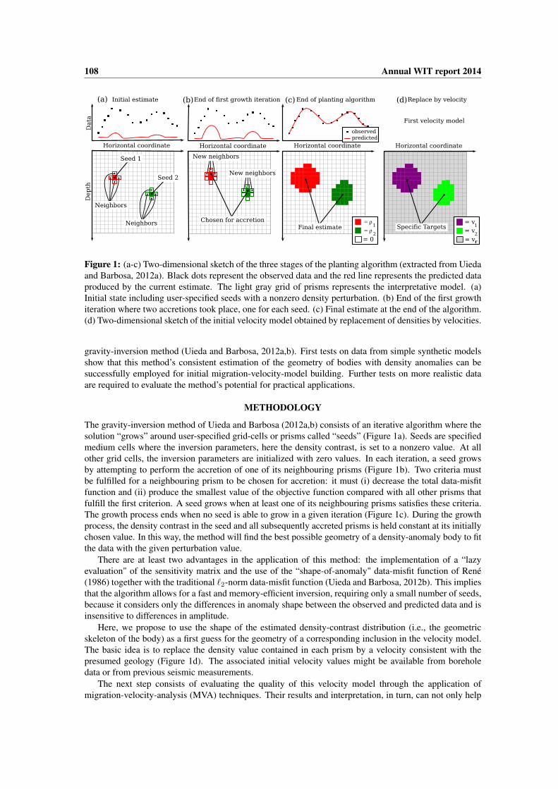
Figure 1: (a-c) Two-dimensional sketch of the three stages of the planting algorithm (extracted from Uiedaand Barbosa, 2012a). Black dots represent the observed data and the red line represents the predicted dataproduced by the current estimate. The light gray grid of prisms represents the interpretative model. (a)Initial state including user-specified seeds with a nonzero density perturbation. (b) End of the first growthiteration where two accretions took place, one for each seed. (c) Final estimate at the end of the algorithm.(d) Two-dimensional sketch of the initial velocity model obtained by replacement of densities by velocities.

gravity-inversion method (Uieda and Barbosa, 2012a,b). First tests on data from simple synthetic modelsshow that this method’s consistent estimation of the geometry of bodies with density anomalies can besuccessfully employed for initial migration-velocity-model building. Further tests on more realistic dataare required to evaluate the method’s potential for practical applications.

METHODOLOGY

The gravity-inversion method of Uieda and Barbosa (2012a,b) consists of an iterative algorithm where thesolution “grows” around user-specified grid-cells or prisms called “seeds” (Figure 1a). Seeds are specifiedmedium cells where the inversion parameters, here the density contrast, is set to a nonzero value. At allother grid cells, the inversion parameters are initialized with zero values. In each iteration, a seed growsby attempting to perform the accretion of one of its neighbouring prisms (Figure 1b). Two criteria mustbe fulfilled for a neighbouring prism to be chosen for accretion: it must (i) decrease the total data-misfitfunction and (ii) produce the smallest value of the objective function compared with all other prisms thatfulfill the first criterion. A seed grows when at least one of its neighbouring prisms satisfies these criteria.The growth process ends when no seed is able to grow in a given iteration (Figure 1c). During the growthprocess, the density contrast in the seed and all subsequently accreted prisms is held constant at its initiallychosen value. In this way, the method will find the best possible geometry of a density-anomaly body to fitthe data with the given perturbation value.

There are at least two advantages in the application of this method: the implementation of a “lazyevaluation" of the sensitivity matrix and the use of the “shape-of-anomaly" data-misfit function of René(1986) together with the traditional `

2

-norm data-misfit function (Uieda and Barbosa, 2012b). This impliesthat the algorithm allows for a fast and memory-efficient inversion, requiring only a small number of seeds,because it considers only the differences in anomaly shape between the observed and predicted data and isinsensitive to differences in amplitude.

Here, we propose to use the shape of the estimated density-contrast distribution (i.e., the geometricskeleton of the body) as a first guess for the geometry of a corresponding inclusion in the velocity model.The basic idea is to replace the density value contained in each prism by a velocity consistent with thepresumed geology (Figure 1d). The associated initial velocity values might be available from boreholedata or from previous seismic measurements.

The next step consists of evaluating the quality of this velocity model through the application ofmigration-velocity-analysis (MVA) techniques. Their results and interpretation, in turn, can not only help

Annual WIT report 2014 109

to improve the velocity values, but can also allow to extract information that helps to improve on thegeometry for the next gravity inversion, thus forming a joint method.

BENEFITS AND DRAWBACKS OF A JOINT METHOD

All geophysical inversion methods are ambiguous, that is, they allow for more than one possible solution toa given problem. Fortunately, for those more traditional methods the ambiguity is, in general, well known.In other words, a geophysicist knows the peculiar limitations of each method and should consider them inall steps of a geophysical work.

One way to minimize ambiguity is by a combination of methods whose ambiguities are quite distinct.For example, in a very simple way, seismic methods generally are more ambiguous in the lateral direc-tion, whereas potential field methods are typically more ambiguous with respect to the vertical direction.Through the combination of these methods it is possible to restrict the problem to a small (and plausible)number of solutions that satisfy both methods.

In this work, we propose a joint method that involves a new three-dimensional gravity inversion tech-nique and seismic MVA techniques for the estimation of geometry, density and velocity of specific targets.The benefits of this joint method are:

1. The forward modeling, processing and inversion of gravimetric data are several times faster than forseismic data, particularly in the 3D case.

2. This allows us to quickly perform many tests for different parameters or even source/targets struc-tures at different scales.

3. Through traditional gravimetric processing/interpretation, we are able to estimate the lateral dimen-sion, limits, and the center of mass for the most prominent structures.

4. This can be improved by the use of gravity-gradient components allowing the determination ofsmaller bodies.

5. Also, it helps to reduce the processing time by restricting the model to the area of interest.

6. Moreover, the gravimetric inversion improves the knowledge of regions where the quality of theseismic image is limited by the effects of wavefield transmission, scattering and absorption, as forexample in salt structures and sub-salt sediments.

7. Vice versa, we can use the knowledge of the upper limit of a body obtained with good precisionfrom routine seismic processing, to reduce the mesh of the gravimetric inversion and to give us moreprecise locations to plant the seeds.

The largest benefit of joint inversion is that the amount of information increases with the integrationof different methods. However, it must be kept in mind that all considerations and restrictions weighedindividually on each method must now be analyzed jointly. This is one of the main difficulties encounteredin joint methods. Unfortunately, problems frequently arise because of severe simplifications. Among themost important difficulties are a poor signal-to-noise ratio (SNR) and the need to ensure that the physicaland geometrical parameters meet the employed geophysical methods not only jointly, but also individuallywhile at the same time being consistent with geology.

To evaluate the feasibility of our proposed joint method, we modeled the gravimetric effect of several3D bodies with different geometries and different densities while jointly producing similar 2D seismicmodels that simulate slices of the three-dimensional model. By means of these models, we performed therobust gravity inversion and 2D depth-migration for the seismic data using the velocity models constructedas previously described. Further, we evaluated both methods with respect to different SNR. Our resultsindicate the capacity of the proposed velocity-model-building technique to generate initial velocity modelsfor migration velocity analysis, including those for specific geological targets (see also Santos et al., 2013,2014b).


APPLICATION TO SYNTHETIC DATA

We tested if the geometry of complex structures such as salt structures obtained by gravity inversion issufficiently well approximated to build a seismic velocity model. As in Santos et al. (2013, 2014b), weperformed an inversion of some 3D bodies with different geometries. To demonstrate the capability of thetechnique, we extracted 2D profiles from the inverted solution, and replaced the density value by a con-sistent and convenient velocity. Thereafter, we performed 2D depth-migration for seismic data previouslymodeled with the real geometry using the velocity model of each extracted profile.

For the forward modeling of the gravity data, we used the formulas of Nagy et al. (2000). Togetherwith the inversion method of planting anomalous density seeds (Uieda and Barbosa, 2012a,b), these for-mulas are implemented in the toolkit Fatiando a Terra (Portuguese for “Slicing the Earth”) of Uieda et al.(2013, 2014), a freely available open-source Python package for modeling and inversion in geophysics. Toperform the necessary seismic processing, we used the open-source software package Madagascar (Fomelet al., 2013).

Ellipsoidal Model

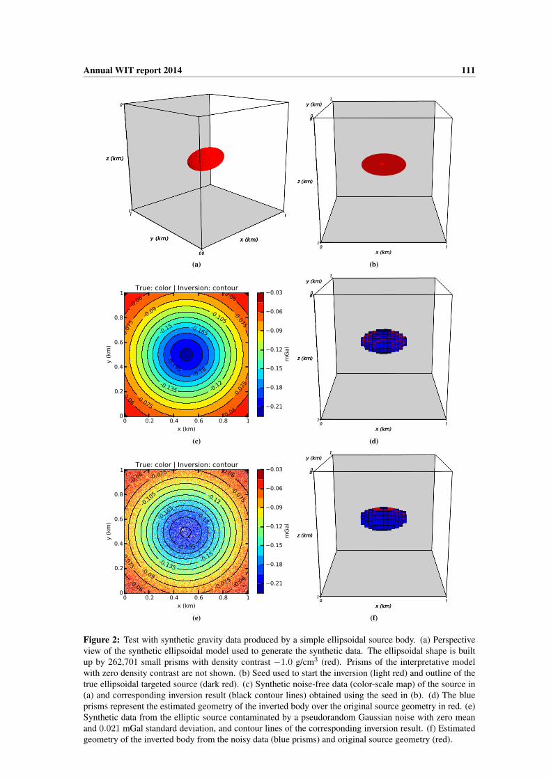
Gravimetric modeling and inversion methods usually use prismatic bodies in their process, which is defi-nitely not useful to achieve our main goal of getting reasonable estimates of the irregular salt body geometrythrough gravimetric measurements. Therefore, the method employed here allows for irregular shapes byaccreting grid cells to the seed body as needed. For our first numerical test, we created a 3D ellipsoid saltbody with half axes of 400 m in the x-direction, and 200 m in the y and z directions (Figure 2(a)).

The gravimetric data were generated considering the density contrast of the source body equal to�1.0 g/cm3. The gz component was calculated on a regular grid of 251 ⇥ 251 observation points inthe x and y directions, totaling 63,001 observations, with a grid spacing of 4 m in both directions (seethe color-scale map in Figure 2(c)). The data were polluted with pseudorandom Gaussian noise with zeromean and 0.021 mGal standard deviation, that is, 0.1% of the absolute amplitude (see the color-scale mapin Figure 2(e)).

In a tentative to evaluate the robustness of the gravimetric inversion method, we set only one seed(Figure 2(b)), at 500 m depth at the center of the simulated body. Both inversions, for the noise-free(Figure 2(c)) and noisy data (Figure 2(e)), were performed using an interpretative model consisting of108,000 rectangular prisms.

The systematic accretion of prisms was controlled by a compactness of µ = 0.1 and a threshold of� = 0.0001. The first is a regularization parameter for the objective function and the second is a smallpositive constant that controls how much the solution is allowed to grow (see Uieda and Barbosa (2012b)for more details).

The black contour lines in Figures 2(c) and 2(e) represent the calculated gz-component data producedby the estimated density-contrast distribution shown in Figures 2(d) and 2(f) (blue prisms). We see thatboth data are satisfactorily inverted, the predicted (blue) prisms being enclosed in the red outline of theoriginal source. As expected, we note a better adjustment in the noise-free test (Figure 2(d)) than in thenoisy-data test (Figure 2(f)). However, this difference does not seem significant.

Next, we used these inverted density-anomaly geometries for seismic processing. Because of computa-tional restrictions, we considered a 2D slice of the 3D model. For the numerical experiment, we considereda velocity model which consists of a 200 m deep water layer, a constant-vertical-gradient background ve-locity (initial velocity of 2000 m/s, gradient of 1.25 1/s), and an elliptic salt body with velocity of 4000 m/s(Figure 3(e)). This 2D longitudinal slice was used to generate the synthetic data to be used in the migrationtests. We carried out time-domain finite-difference vector-acoustic modeling. The source signature was a30 Hz Ricker wavelet sampled with a time-step of 0.2 ms, Total recording time was 0.8 s. The data wasresampled later on to 4 ms. We fired 42 shots at 50 m depth, spaced by 24 m, spanning a distance from 0to 984 m.

On these synthetic data, we performed extended split-step Fourier migrations, using the first 75 fre-quencies with a frequency sampling of 1.16 Hz, with four different models: (i) constant (water) velocityequal 1500 m/s (model in Figure 3(a), migrated image in Figure 3(b)), where the sea floor is correctlypositioned, but the salt body is misplaced; (ii) background-gradient model (model in Figure 3(c), migrated


(a) (b)

(c) (d)

(e) (f)

Figure 2: Test with synthetic gravity data produced by a simple ellipsoidal source body. (a) Perspectiveview of the synthetic ellipsoidal model used to generate the synthetic data. The ellipsoidal shape is builtup by 262,701 small prisms with density contrast �1.0 g/cm3 (red). Prisms of the interpretative modelwith zero density contrast are not shown. (b) Seed used to start the inversion (light red) and outline of thetrue ellipsoidal targeted source (dark red). (c) Synthetic noise-free data (color-scale map) of the source in(a) and corresponding inversion result (black contour lines) obtained using the seed in (b). (d) The blueprisms represent the estimated geometry of the inverted body over the original source geometry in red. (e)Synthetic data from the elliptic source contaminated by a pseudorandom Gaussian noise with zero meanand 0.021 mGal standard deviation, and contour lines of the corresponding inversion result. (f) Estimatedgeometry of the inverted body from the noisy data (blue prisms) and original source geometry (red).


(a) (b)

(c) (d)

(e) (f)

(g) (h)

Figure 3: Migrations for elliptic salt body using three different velocity models (left column) and theircorresponding depth migrated images (right column): (a) and (b) for a constant velocity model of 1500 m/s.(c) and (d) for the background gradient model; (e) and (f) for the true velocity model; (g) and (h) for initialvelocity model obtained by attributing salt velocity to the geometry of the inverted gravity anomaly.

image in Figure 3(d)), where we see that the sea floor and top-of-salt were correctly imaged, and the bottomof the salt was delineated but has wrong amplitude and is incorrectly positioned; (iii) true model (model inFigure 3(e), migrated image in Figure 3(f)), to provide a reference image of the top and bottom of the body;(iv) velocity model created using the gravity inversion, considering a 2D longitudinal slice of the predictedresult of the noisy-data test (Figure 2(d)). Figure 3(g) and 3(h) show the velocity model and the migratedimage, respectively. Even for this unsmoothed velocity model, we observe that the resulting image is in


Figure 4: Pluto stratigraphic velocity model. We used the right-most part beyond x = 23000 m down to adepth of 8000 m.

agreement with the one obtained using the true velocity, including the amplitude difference between topand bottom of the salt body. From the incorrect images in Figures 3(b) or 3(d), it is possible to estimatewhere to place a first trial seed for the gravity inversion.

Pluto Model

For a more realistic test, we used the right part of the 2D Pluto model (see Figure 4). The Pluto datasetis one of several test sets released by The Subsalt Multiples Attenuation and Reduction Technology JointVenture (SMAART JV). It is designed to emulate deep water subsalt prospects as found in the Gulf ofMexico.

From this model we created a 3D salt body to be used in the gravimetric modeling (see Figure 5(a)). Tocreate this 3D body from the 2D model, we proceeded in the following way:

• We extracted the 2D salt body by masking the 2D Pluto model with the proper velocity (4500 m/s).This is the central slice of the yet-to-be 3D salt body.

• We then extrapolated the 2D slice laterally in the y-direction by concatenating to both sides a setof modified slices. Each slice to be concatenated was smoothed with increasing window and thenmasked again with the same velocity value as before. This created slices with decreasing areas ascan be seen in Figure 5(a).

For the gravimetric modeling, we discretized the so-constructed 3D salt body using 120,960 small prismswith density contrast �0.3 g/cm3 (Figure 5(a)). The modeled gz-component is depicted by the color-scale map in Figure 5(c). It was calculated on a regular grid of 151 ⇥ 115 observation points in the x-and y-directions, totaling 17,365 observations, with a grid spacing of 53.34 m in both directions. Wethen contaminated these modeled data with pseudorandom Gaussian noise with zero mean and 0.1 mGalstandard deviation. As for the first example, we used only a single seed at the center of the simulated body(i.e., at x = 4500 m, y = 3000 m, and z = 3000 m, see Figure 5(b)) to start the gravimetric inversion,which was performed considering an interpretative model consisting of a regular grid of 128,000 prisms,with µ = 0.1 and � = 0.0001. The black contour lines in Figure 5(c) show the predicted data of thegz-component produced by the estimated density-contrast distribution (blue prisms in Figure 5(d)). We seethat the predicted density distribution fits with the original source structure in all directions.

For the seismic evaluation, we again performed extended split-step Fourier migrations. We used theavailable Pluto model shot records, sampled at 8 ms. Out of the available 694 shots, we used 51. Theirpositions are indicated as red stars in all velocity models in this section. The shots were located at 7.62 mdepth and are spaced at 137.16 m. We used 150 equally spaced frequencies from 8.0 Hz to 40.4 Hz in themigration process.

For a detailed analysis of the velocity-building process, we migrated the data with five velocity models:(i) constant (water) velocity equal 1500 m/s (Figure 6); (ii) constant vertical-gradient velocity obtained by


(a) (b)

(c) (d)

Figure 5: Application to the Pluto salt model. (a) Perspective view of the synthetic salt structure usedto generate the gravity data. The salt shape is built by accretion of 120,960 small prisms with densitycontrast �0.3 g/cm3 (red). Prisms of the interpretative model with zero density contrast are not shown.(b) Seed used to start the inversion (light red) and outline of the true salt targeted source (dark red). (c)Synthetic data with noise (color-scale map) and its corresponding predicted data by the inversion result(black contour lines). The data were contaminated by pseudorandom Gaussian noise with zero mean and0.1 mGal standard deviation. (d) Estimated geometry of the inverted body (blue) together with originalsource geometry (red).

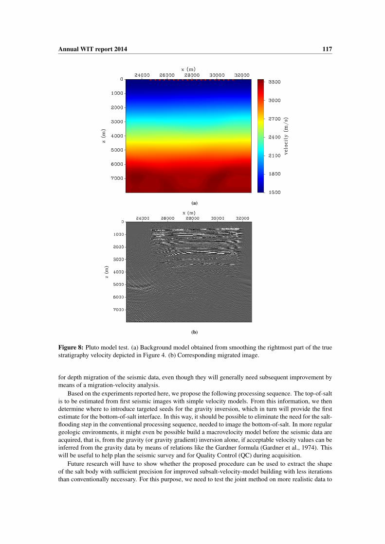
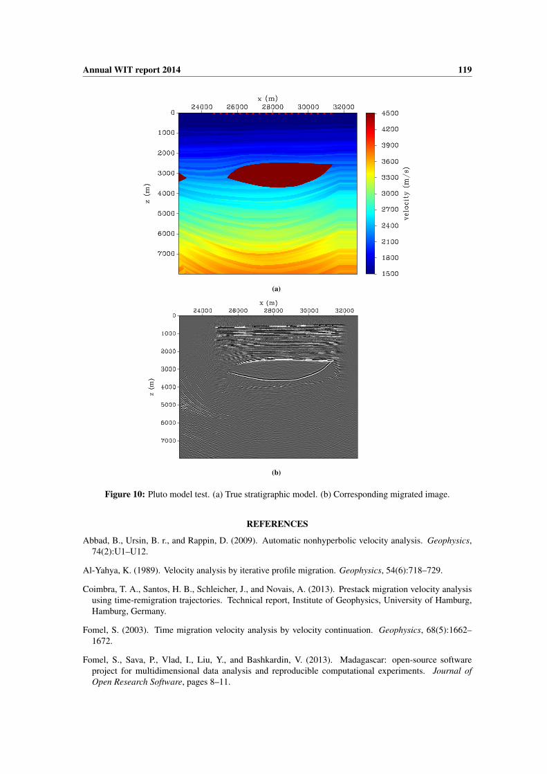
the function v(z) = (1500 + 0.235z) m/s (Figure 7); (iii) smoothed background with no salt body createdusing the true stratigraphy velocity (Figure 8); (iv) velocity model obtained by replacement of the den-sity value contained in each prism by a velocity consistent with the presumed geology superimposed ontothe above background model (Figure 9). Here we set the velocity inside the predicted body to 4500 m/ssurrounded by smoothed values of the true model; (v) true stratigraphic velocity of the Pluto model (Fig-ure 10).

The migrated images presented in these figures prove that imaging the bottom of salt structures is nota simple task, even if we have a sediment model close enough to the real scenario, such as the smoothedbackground velocity model in Figure 8(a). On the other hand, all these “wrong” results demonstrate thepossibility to estimate the top of salt by means of very simple velocity models. Although it is true that theycarry errors in the vertical position, any of these initial estimates can be used as a first guess to guide the


(a)

(b)

Figure 6: Pluto model test. (a) Constant velocity model with water velocity 1500 m/s. (b) Correspondingmigrated image.

planting of the seeds or to reduce the number of cells in the mesh of the gravity inversion. Once the saltbody has been estimated and inserted into the background model, further migration-velocity analysis canbe used to improve the so-obtained initial model.

Our final result in Figure 9 confirms the quality of the proposed technique. We see that even for thisrough estimate of the salt geometry, the resulting velocity model (Figure 9(a)) used for depth-migration(Figure 9(b)) resulted in a satisfactory migrated image of the salt bottom (compare with the image fromthe true model in Figure 10(b)). We emphasize that for the salt-geometry estimation, we made use of thesimplest possible version of the gravity inversion procedure. It used only one iteration with a single seed,without any previous information or preprocessing.

If this simplistic procedure fails, it can be improved in different aspects. It is possible to add moreinformation for the first inversion of gravimetric data, in the form of a more instructed distribution of seeds.To the same end, we can iterate the gravimetric inversion, until the resulting velocity model is acceptablefor seismic migration. In each iteration, we can make use of the geometry information from previousiterations to improve our guess for the spacial position of the seeds. Of course, geometric information from


(a)

(b)

Figure 7: Pluto model test. (a) Constant-gradient velocity model. (b) Corresponding migrated image.

intermediate migrations can also be used to improve the seed positioning.

CONCLUSION

We have studied 3D velocity model building making use of information from gravity inversion. The par-ticular inversion method used is based on planting seeds of anomalous densities and letting the resultingbodies grow. This inversion method has been proven to be efficient in estimating a 3D density-contrast dis-tribution on a grid of prisms. For this purpose, it does not require the solution of a large equation system,which greatly reduces the computational demand.

For its use in seismic migration, we extracted the geometrical skeleton of the inverted body and filledeach prism with a velocity consistent with the presumed geology. Because of the very fast construction ofthe anomalous body, this procedure is an attractive way to improve the knowledge of complex structures,for example, salt structures and sub-salt sediments, in regions of large velocity contrasts, where the seismicimaging is limited by the effects of wavefield transmission, scattering and absorption. Tests on severalsynthetic data demonstrated the capability of our method to construct initial velocity models that are useful


(a)

(b)

Figure 8: Pluto model test. (a) Background model obtained from smoothing the rightmost part of the truestratigraphy velocity depicted in Figure 4. (b) Corresponding migrated image.

for depth migration of the seismic data, even though they will generally need subsequent improvement bymeans of a migration-velocity analysis.

Based on the experiments reported here, we propose the following processing sequence. The top-of-saltis to be estimated from first seismic images with simple velocity models. From this information, we thendetermine where to introduce targeted seeds for the gravity inversion, which in turn will provide the firstestimate for the bottom-of-salt interface. In this way, it should be possible to eliminate the need for the salt-flooding step in the conventional processing sequence, needed to image the bottom-of-salt. In more regulargeologic environments, it might even be possible build a macrovelocity model before the seismic data areacquired, that is, from the gravity (or gravity gradient) inversion alone, if acceptable velocity values can beinferred from the gravity data by means of relations like the Gardner formula (Gardner et al., 1974). Thiswill be useful to help plan the seismic survey and for Quality Control (QC) during acquisition.

Future research will have to show whether the proposed procedure can be used to extract the shapeof the salt body with sufficient precision for improved subsalt-velocity-model building with less iterationsthan conventionally necessary. For this purpose, we need to test the joint method on more realistic data to


(a)

(b)

Figure 9: Pluto model test. (a) Model obtained from insertion of a salt body with the geometry fromgravity inversion into the background model of Figure 8(a). (b) Corresponding migrated image.

evaluate the computational cost in the presence of more complex and realistic geology like deep marinesalt bodies, with hydrocarbon reservoirs, salt feeders, channels, faults, internal sutures and heterogeneoussalt cap and many others important structures that are challenges for geophysical prospection.

ACKNOWLEDGMENTS

This research was supported by Petrobras and CGG as well as the Brazilian national research agenciesCNPq, FAPESP, and CAPES. The first author (HBS) thanks CGG-Brazil for his fellowship, the secondauthor (DLM) thanks Schlumberger-Brazil for his fellowship, and the third author (EBS) thanks CAPESfor his fellowship. Additional support for the authors was provided by the sponsors of the Wave InversionTechnology (WIT) Consortium. We acknowledge Leonardo Uieda for discussions and insightful com-ments. We would like to thank the use of plotting library matplotlib by Hunter (2007) and software Mayaviby Ramachandran and Varoquaux (2011). We thank the SMAART JV for providing the Pluto dataset.


(a)

(b)

Figure 10: Pluto model test. (a) True stratigraphic model. (b) Corresponding migrated image.

REFERENCES

Abbad, B., Ursin, B. r., and Rappin, D. (2009). Automatic nonhyperbolic velocity analysis. Geophysics,74(2):U1–U12.

Al-Yahya, K. (1989). Velocity analysis by iterative profile migration. Geophysics, 54(6):718–729.

Coimbra, T. A., Santos, H. B., Schleicher, J., and Novais, A. (2013). Prestack migration velocity analysisusing time-remigration trajectories. Technical report, Institute of Geophysics, University of Hamburg,Hamburg, Germany.

Fomel, S. (2003). Time migration velocity analysis by velocity continuation. Geophysics, 68(5):1662–1672.

Fomel, S., Sava, P., Vlad, I., Liu, Y., and Bashkardin, V. (2013). Madagascar: open-source softwareproject for multidimensional data analysis and reproducible computational experiments. Journal ofOpen Research Software, pages 8–11.


Gardner, G. H. F., Gardner, L. W., and Gregory, A. R. (1974). Formation velocity and density—the diag-nostic basics for stratigraphic traps. Geophysics, 39(6):770–780.

Hunter, J. D. (2007). Matplotlib: A 2D graphics environment. Computing in Science and Engineering,9(3):90–95.

Liu, Z. (1997). An analytical approach to migration velocity analysis. Geophysics, 62(4):1238–1249.

Liu, Z. and Bleistein, N. (1995). Migration velocity analysis: Theory and an iterative algorithm. Geo-physics, 60(1):142–153.

Mulder, W. a. and ten Kroode, a. P. E. (2002). Automatic velocity analysis by differential semblanceoptimization. Geophysics, 67(4):1184–1191.

Nagy, D., Papp, G., and Benedek, J. (2000). The gravitational potential and its derivatives for the prism.Journal of Geodesy, 74(7-8):552–560.

Ramachandran, P. and Varoquaux, G. (2011). Mayavi: 3D Visualization of Scientific Data. Computing inScience & Engineering, 13(2):40–51.

René, R. M. (1986). Gravity inversion using open, reject, and "shape-of-anomaly" fill criteria. Geophysics,51(4):988–994.

Santos, H. B., Coimbra, T. A., Schleicher, J., and Novais, A. (2014a). Prestack time-migration velocityanalysis using remigration trajectories. Geophysics. Submitted.

Santos, H. B., Macedo, D. L., Santos, E. B., Schlecher, J., and Novais, A. (2014b). Specific target deter-mination by planting anomalous densities applied to seismic migration-velocity improvements. In EGUGeneral Assembly Conference Abstracts, volume 16, page 15671.

Santos, H. B., Macedo, D. L., Santos, E. B., Schleicher, J., and Novais, A. (2013). Construction of aninitial velocity model for migration velocity analysis from gravimetric inversion. In AGU Fall Meeting,pages Abstract S41D–06, San Francisco, US.

Schleicher, J. and Costa, J. C. (2009). Migration velocity analysis by double path-integral migration.Geophysics, 74(6):WCA225–WCA231.

Schleicher, J., Costa, J. C., and Novais, A. (2008). Time-migration velocity analysis by image-wave prop-agation of common-image gathers. Geophysics, 73(5):VE161–VE171.

Uieda, L. and Barbosa, V. C. F. (2012a). Robust 3D gravity gradient inversion by planting anomalousdensities. Geophysics, 77(4):G55.

Uieda, L. and Barbosa, V. C. F. (2012b). Use of the "shape-of-anomaly" data misfit in 3D inversionby planting anomalous densities. In SEG Technical Program Expanded Abstracts 2012. Society ofExploration Geophysicists.

Uieda, L., Oliveira Jr, V. C., and Barbosa, V. C. F. (2013). Modeling the Earth with Fatiando a Terra. InProceedings of the 12th Python in Science Conference.

Uieda, L., Oliveira Jr, V. C., Ferreira, A., Santos, H. B., and Caparica Jr, J. F. (2014). Fatiando a terra: APython package for modeling and inversion in geophysics. Figshare.

Zhu, J., Lines, L., and Gray, S. (1998). Smiles and frowns in migration/velocity analysis. Geophysics,63(4):1200–1209.

use of 3d gravity inversion to aid seismic migration...

Documents