tomographic inversion of reflection seismic amplitude … · · 2016-04-20tomographic inversion...

Geophys. J . Int. (1995) 123,355-372

Tomographic inversion of reflection seismic amplitude data for velocity variation

Yanghua Wang'* and Gregory A. 'Houseman2 Department of Earth Sciences, Monash University, Clayton, Victoria 3168, Australia

'Department of Mathematics & Australian Geodynamics Cooperatioe Research Centre, Monash University, Clayton, Victoria 31 68, Australia

Accepted I995 April 11. Received 1995 April 4; in orignal form 1994 September 16

SUMMARY Inclusion of amplitude data in reflection seismic tomography may help to resolve the ambiguity caused in the traveltime inversion by the trade-off between reflector position and velocity anomaly. To illustrate the uses of amplitude data we initially exclude all traveltime information from the inversion. In a previous paper (Wang & Houseman 1994) we have shown, using geologically relevant synthetic models, that the information contained in amplitude versus offset data suffices to accurately constrain the geometry of an arbitrary smooth 2-D reflector separating constant velocity layers. In this paper we investigate the implementation of the inversion for 2-D velocity variations using reflection seismic amplitude data.

A stable method of ray tracing in a 3-D heterogeneous velocity medium is presented. The ray-geometric spreading which partly determines the ray amplitude is then calculated according to the propagator along the ray path. The ray-perturbation theory is used to trace the perturbed ray due to the model perturbation. We compare amplitude perturbations arising from slowness perturbations along the whole ray path with those arising from the slowness perturbation close to the interface, and see that in an inversion of reflection seismic amplitude data, the data residuals will have most effect on velocity anomalies near the interface. Synthetic models are used to demonstrate the efficacy of amplitude inversion for velocity variation, using the subspace inversion method, with a 2-D Fourier series parametrization of the slowness distribution. The efficiency of the inversion lies in a judicious partitioning of model parameters into subspaces. A stable strategy for the parameter partitioning is to separate parameters on the basis of the magnitude of rms values of the Frechet derivatives of ray amplitudes with respect to the model parameters. Numerical examples show that the amplitudes of reflected signals are sensitive to the location of the velocity anomalies. Inversions provide an approximate image of velocity variation, demonstrating that amplitude data contain information that can constrain unknown velocity variation.

Key words: amplitude inversion, ray-geometric spreading function, ray-perturbation theory, tomography.

1 INTRODUCTION

In reflection seismic tomography using only traveltime data there may be an ambiguity in the solution in the form of a trade- off between reflector depth and velocity anomaly (Williamson 1990;Blundell 1992; Stork & Clayton 1992). It may not be possible to resolve this ambiguity using only traveltime information, par- ticularly if the velocity anomaly is close to the reflector

'Now at: Department of Geology, Imperial College of Science, Technology & Medicine, University of London, Prince Consort Road, London SW7 2BP. UK.

(Williamson 1990). The inclusion of amplitude data in the inversion may help to resolve the ambiguity. Our aim here is to investigate the use of simplified seismic amplitude data in order to improve on the result of traveltime inversion. We anticipate that the additional information will provide better velocity resolution than is possible with traveltime data alone, without excessive computational time. In a previous paper (Wang & Houseman 1994) we explored the use of amplitude data to invert models containing variable geometry reflectors separating constant velocity layers. In this paper we will investigate the tomographic inversion of amplitude data for 2-D continuously varying velocity with a known reflector geometry.

0 1995 RAS 355

at Imperial C

ollege London on D

ecember 15, 2014

http://gji.oxfordjournals.org/D

ownloaded from

http://gji.oxfordjournals.org/

356 Y. Wung and G. A. Houseman

To illustrate the information content of amplitude data we exclude traveltime information from the inversion examples we show below. We use the concept of ray amplitude in the high-frequency approximation, assuming that the amplitude of a propagating pulse in a non-dissipative medium depends on the geometry of the ray tube and local reflectionJtransmission coefficients at interfaces, and is unaffected by intrinsic anelastic attenuation. By this assumption the set of amplitude data scales linearly with source amplitude, which is arbitrary. For tomographic inversion, the information content of the data lies in the dependence of signal amplitude on source-receiver offset. If attenuation is important in real data, these methods would need re-examination. But if the pulse shapes are not significantly altered by attenuation, the simplified amplitude data could still be used, in principle, to provide constraints on velocity inversion. Even if there is no attenuation, the amplitude of reflected or transmitted pulses may be frequency-dependent for waves incident on thin layers (e.g. MacDonald, Davis & Jackson 1987), but we assume here the infinite-frequency amplitude obtained from the geometrical ray-amplitude calculation (Cerveny & Ravindra 1971).

Ray-amplitude data have previously been used in velocity inversion by Thomson (1983), Nowack & Lutter (1988) and Nowack & Lyslo (1989). Thomson (1983) and Nowack & Lutter (1988) used the amplitude of direct arrivals to invert for velocity variation. Using a slightly perturbed model in which the velocity of two smoothly splined velocity heterogen- eities is increased by 1 per cent above a constant background, Nowack & Lyslo (1989, Fig. lob) showed that it is possible to invert for velocity variation using reflection seismic amplitudes. This is apparently the only published example of velocity inversion based on ray amplitude of reflection seismic data, so further investigation of this topic is required.

In a ray-path-based tomographic inversion it is necessary to have a robust ray-tracing routine. We present a bending method, for the two-point ray tracing within a 3-D heterogeneous velocity structure, based on Fermat’s principle (cf. Moser, Nolet & Snieder 1992). This method reduces to the iterative solution of a linearized tridiagonal equation system (Appendix A). In Section 2 we describe the calculation of ray amplitudes where ray-geometric spreading is determined using the propagator of paraxial rays (Thomson & Chapman 1985). The paraxial ray parameters can be determined by solving a linearized ray-equation system, whose solution is analytically expressed in terms of propagator matrices as a function of ray parameter along the central ray (Gilbert & Backus 1966; Aki & Richards 1980). When a slowness discontinuity exists, appropriate continuity conditions have to be introduced. By modifying the method of Farra, Virieux & Madariaga (1989) for the ray-amplitude calculation, we derive a complete formula for the linear transformation of propagator matrices across a smooth interface (Appendix B). In Section 3 we describe, using ray-perturbation theory (cf. Farra & Madariaga 1987), the determination of the ‘two-point’ perturbation to the central ray and paraxial rays caused by the slowness perturbation. We use finite differences to calculate the Frechet matrix of derivatives describing the perturbation of amplitude arising from variation of the model slowness parameters, in the general non-linear case.

As the focus of this study is the use of tomographic inversion methods in reflection seismology, we work with a model parametrization in which the subsurface velocity distribution

consists of layers within which velocity varies continuously, separated by surfaces across which the velocity changes discon- tinuously. In the examples, we invert for an unknown velocity distribution in a single layer, bounded below by a horizontal reflection surface (planar). Within a layer the velocity distribution is parametrized using a 2-D Fourier series. In Section 4 we show, by means of a numerical comparison, that the amplitude of a reflected wave is more sensitive to the slowness perturbation in the vicinity of the reflection point than to a comparable perturbation at any other point on the ray path. Therefore, even though some quite good results have been obtained from inversion of the amplitude data of direct seismic arrivals (e.g. Nowack & Lutter 1988), it is difficult to reconstruct interval velocity variation from amplitude of reflected arrivals because of this property. Singular value analysis shows that amplitude data are most sensitive to the short-wavelength Fourier components of the velocity model.

Finally we present examples of the inversion for velocity variation of synthetic reflection seismic amplitude data, using the subspace inversion method. The subspace method is ideally suited to the problem in which the model space includes parameters of different dimensionality. Kennett, Sambridge & Williamson (1988), and Williamson (1990) and Sambridge ( 1990) have applied this method to various traveltime inversion problems. However, even when all parameters have the same physical dimension, appropriate partitioning of different parameter components into separate subspaces may be effective in accelerating convergence and obtaining an accurate solution (Wang & Houseman 1994). In the amplitude inversions presented in this paper we partition the parameters into different subspaces on the basis of the different sensitivities of the ray- amplitude values with respect to the model parameters. We demonstrate the application of reflection seismic amplitude inversion for velocity variation using synthetic data sets obtained from a range of simple models with 2-D velocity variation.

2 MODEL PARAMETRIZATION A N D RAY-AMPLITUDE CALCULATION

2.1 Parametrization of slowness variation

For ray-amplitude calculations the model slowness distribution must vary smoothly within a layer. In a medium with smoothly varying slowness, any ray is composed of an arc with continuously varying curvature. Traveltime and its derivatives with respect to the model parameters can be calculated, and if the ray tube around the reference ray smoothly diverges, calculation of the ray amplitude is also stable.

For the ray-tracing calculations used to generate the synthetic data, a variable slowness field is represented by a set of discrete slowness values on a regular 2-D grid. Slowness within the cells defined by the gridpoints is determined using the bicubic interpolation, so that the values of the function and the specified derivatives change continuously as the interpolat- ing point crosses from one grid cell to another. Bicubic interpolation requires us to specify at each gridpoint not just the slowness function u(x), where x is the Cartesian coordinate, but also the gradient aulax, and the cross derivative a2u/ax, ax,. These derivatives at each gridpoint are determined by centred finite difference of the values of u on the grid.

While the ray-tracing requires a densely sampled slowness

0 1995 RAS, GJI 123, 355-372

at Imperial C

ollege London on D

ecember 15, 2014


ownloaded from


Inversion of reflection seismic amplitude data 351

distribution, the inversion procedure must be designed to get solutions for long-wavelength slowness variation, and avoid the computational instability that can occur where short wavelength variations in slowness are permitted. Therefore, in the inversions described below, we use a truncated 2-D Fourier series representation of the slowness field within a given layer rather than the cell representation frequently used in traveltime tomography:

u = 1 [aijcos(iAknx)cos( jAknz) N N

i = o j = o

+ bijsin(iAknx)cos( jAknz)

+ cijcos(iAknx) sin( jAknz)

+ di,sin(iAknx) sin( jAknz)] ,

where a, b, c and d with subscripts i and j are amplitude coefficients of the (i, j) th harmonic term and N is the number of harmonic terms in each dimension. The wavenumbers in the series are defined as integer multiples of the fundamental wavenumber Ak. For a given velocity field, eq. (1) can be used to construct the regular mesh of constant slowness values used in the ray tracing (Appendix A).

At an interface between layers, the assumption of a smooth interface (i.e. the existence of its partial derivatives of the first and second order) is necessary in order to calculate the transformation of the ray and paraxial rays. Energy partitioning due to reflection or transmission at the interfaces and the effects of focusing and defocusing of the ray tube at interfaces are the crucial factors in the determination of ray amplitude in a reflection seismogram (Wang & Houseman 1994). In Appendix B we derive the expression for the complete transformation of the ray tube on a curved interface, but for the inversion examples here, we assume that the reflection surface is horizontal and planar, in order to separate the influence of reflector curvature and internal velocity variation.

2.2 Propagator of paraxial rays

The analysis of this section follows that of previous authors (Thomson & Chapman 1985; Farra, Virieux & Madariaga 1989 Virieux 1991), but is summarized here in order to explain the modifications to the theory introduced in this paper. In the high-frequency approximation, the elastodynamic equation yields a non-linear first-order partial differential equation for the traveltime T which is called the eikonal equation,

where u is the slowness and x is the position vector. Denoting p = V T, the conjugate momentum of x, as the slowness vector, a ray trajectory is defined as a curve described in the position x and momentum p by the canonical vector yT(a) = [x(a), p(a)], where a is an independent variable which we define by uda = ds, and s is arclength. Introducing the Hamiltonian, we can write the ray-tracing equations as

ir=VpH,

p = -V,H, (3)

where the dot indicates derivative with respect to a (Cerveny, Molotkov & Psencik 1977; Cerveny 1985). The Hamiltonian function associated with the above definition for the

independent variable a is

H(x, P, 0) = fCp2 - u2(x)I . (4)

This expression for the Hamiltonian was proposed by Burridge (1976). Thomson & Chapman (1983, Cerveny (1985), and Kendall & Thomsoa (1989) discuss various expressions for the Hamiltonian.

Suppose a ray has been traced in the medium with slowness distribution u using the ray-tracing algorithm described in Appendix A, and denote y:(a) = [&(a), p,(a)] the canonical vector of that reference ray. Around this ray we can obtain paraxial rays by means of first-order perturbation theory (Farra & Madariaga 1987; Virieux, Farra & Madariaga 1988). For rays nearby the central ray, y(a) = y,(a) + 6y(a), where 6yT = [Sx, 6p] is the vector of perturbations to position and slowness relative to the reference ray, the ray equations (3) can be linearized (Thomson & Chapman 1985) and rewritten as

Sy = A6y , ( 5 )

where

- V,V, H - VpVx H *=[ From the Hamiltonian (4) we have

A=[’ u o ‘1, where U is a 3 x 3 symmetric matix with elements

u. = - - + u - . aU au aZu

axi axj axiaxj

The linear ray perturbation equations ( 5 ) can be solved using the standard propagator techniques (Aki & Richards 1980). Any solution, Sy(a), can be written in terms of the propagator n(a, ao) and the initial condition 6y(ao) as

SY(4 = w, 0 0 ) 6Y(ao). (7)

The propagator matrix can be evaluated as an infinite series involving integrals of A along the ray path. Truncating the series at the linear term, the propagator may be approximated by the formula (Gilbert & Backus 1966):

n(a, aO) = n [I + (‘k - uk- l)A(uk)l * (8) k

When the rays hit a discontinuity of zeroth or first order, we have to introduce appropriate boundary conditions for ray tracing (Cerveny 1985; Chapman 1985; Farra et al. 1989). Suppose a central ray yJa) intersects the interface at sampling parameter where the perturbation of canonical vector of the paraxial ray in the incident medium is 6y(ak). Denote variables in the reflected/transmitted ray with a caret above them. The continuity condition for perturbations of the canonical vector 6f(ak) and 6y(ak) across the interface may be expressed in terms of the transformation matrix z(ak) defined by

6f(ak) = E(ak) 6y(ak), (9)

where the matrix E is the product of three transformation matrices, described as the components @, Y and R in

0 1995 RAS, GJI 123, 355-372

at Imperial C

ollege London on D

ecember 15, 2014


ownloaded from


358 Y. Wang and G. A. Houseman

Appendix B. In the paper of Farra et al. (1989) the matrix E consisted of two terms @ and Y only, which is adequate for ray tracing, but for the ray-amplitude calculation must include the third term Q. In Appendix B we derive the expression for the complete transformation. Therefore, the generalized propagator, taking transformation matrices at all M interfaces into account, is given by

I

n(a,uO) = n(a, U M ) n c(ak)n(ok, a k - 1 ) . (10) k = M

Once n(a, g o ) is calculated, the entire set of paraxial rays can be found by adjusting the initial conditions, which have to satisfy the condition 6H = V,H * 6p + V, H * 6x = 0 derived from first-order perturbation of the Hamiltonian (Virieux 1991).

2.3 Ray geometric spreading and ray amplitude

We have obtained the paraxial rays around a central ray. The ray geometric spreading, D, can then be defined by

D = { d e t [ s ] > 1 1 2 .

Introducing the following partition of the propagator into submatrices which act on x and p separately:

the ray geometric spreading can be rewritten as

D = [det(Q, + 1Q2)-J1/*, (13)

6p(u,) = 16x(a,). (14)

where 1 determines the initial shape of the ray beam:

For an initial point source in a constant slowness medium, we have

where uo(ao) is the slowness at a,, and so(ao) is arclength measured from a = 0. For an initial plane wave, however, 1 = 0.

In a non-dissipative system, the ray amplitude in a seismogram is proportional to the inverse of the ray-geometric spreading function D,

where C is the product of reflection and transmission coefficients at the interfaces (Cerveny & Ravindra 1971; Wang & Houseman 1994).

3 P E R T U R B E D R A Y A N D A M P L I T U D E

In the iterative inversion procedure we need to calculate the matrix of the Frechet derivatives of the ray amplitudes with respect to the model parameters. The procedure can be linearized by assuming that the ray paths do not change during the inversion, but this approximation may not be valid for large-amplitude slowness anomalies, in which case it is first necessary to calculate the perturbation to the ray trajectory. In this section we attempt to use the first-order ray-perturbation theory determining the perturbed ‘two-point’ ray in the

perturbed medium. Let u, represent the reference slowness distribution and Au the slowness perturbation. Note that A is used to denote perturbations due to the structure, while 6 is used for paraxial perturbations (previous section) and variables with subscript ‘0’ will correspond to those in the unperturbed reference medium.

3.1 ‘Shooting’ perturbed ray

In the medium with perturbed slowness distribution u(x) = uo + Au(x), where the perturbation Au is a smooth function which is assumed to have continuous second-order derivatives, calculation of the perturbed rays is similar to that of the paraxial rays in the reference medium. The perturbed ray with the canonical vector perturbation Ay(a) may be found by the following linear system (cf. Farra & Madariaga 1987; Farra 1990, 1992; Virieux & Farra 1991),

A9 = A,Ay + AB, (17)

with a source AB(a) containing the Hamiltonian perturbations,

AB=[ - vpAH], V, AH

where the perturbation of the Hamiltonian, AH = -uoAu, if H is defined by eq. (4). And then explicitly, ABT = [0, uoV, Au + AuV,u,]. Eq. ( 17) is similar to eq. ( 5 ) , except for the source term AB. The perturbation Ay(u) of the central ray in the perturbed medium is then obtained by the standard propagator technique (Gilbert & Backus 1966):

Ay(a) = no(a, 00) Ay(ao) + no(a, T) W 7 ) d t 9 (19) L where no(a,ao) is the 6 x 6 propagator matrix of the paraxial system eq. ( 5 ) in the unperturbed medium. The integration term in eq. (19) can be explicitly written as

Ax,(u) = (U - 7)(uoVXAu + AuV,uo)dT, L ApB(a) = [ (uoV. Au + AuV,u,) dt ,

where Ayi(a, a,) = [AxB, ApB] . Upon reflection/transmission of the perturbed ray across an

unperturbed interface, we may approximately calculate the perturbation A3 in the reflected/transmitted ray using eq. (9),

Af(‘k) = zO(ak) 9 (21)

with the transformation matrix Xo(ur) calculated in the unperturbed medium. (Note that the relation of Af(o,) = -Ay(a,) for reflection, used by Nowack & Lyslo (1989), is only correct for normal incidence.)

3.2 ‘Two-point’ perturbed ray

To trace the perturbed trajectory of the central ray with the same initial position vector as the unperturbed ray, we set AyT(a,) = [0, Ap(a,)] in eq. (19), where Ap = (Au/u)p due to slowness perturbation at the source point. The ‘perturbed ray’ will not in general hit the receiver R (see Fig. 1). Assume the perturbed ray hits the receiver level at R*, near R. Denoting the unperturbed ray as I,, the perturbed ray as I * , the

0 1995 RAS, GJI 123,355-372

at Imperial C

ollege London on D

ecember 15, 2014


ownloaded from



S R R f

Figure 1. The geometry of ray perturbation. Suppose I , is an unperturbed ray. I* and I are the ‘shooting’ perturbed ray and the ‘two- point’ perturbed ray respectively, due to slowness perturbation.

perturbation of position vector of the perturbed trajectory I* with respect to the unperturbed central ray lo calculated by eqs (19) and (21) is Ax*(a). The ray we want to obtain is a ‘two-point’ perturbed ray, which is denoted by I , connecting S and R. Referring to Fig. 1, the ‘two-point’ perturbed ray I should be a paraxial ray of the perturbed central ray I*.

The propagator matrix describing the paraxial ray propa- gation around the perturbed ray I* is from the solution of the linear system of eq. ( 5 ) in the perturbed medium with A(a) = &(a) + AA(a). The perturbation of linear system, AA, can be written as AA(a) x AA,(a) + AA2(a), in which AA,(a) is a term due to AH, the perturbation in the Hamiltonian, and AA2(a) is a term due to Ay, the perturbation of the reference central

ray (Farra & Madariaga 1987; Farra 1990):

AA2 = [AxV, + ApV,]Ao.

From eq. ( 6 ) , eq. (22) can be r e w h e n as

0 0 O ] . M , = [ ~ 0 0 O ] .

where the elements of AU and 0 can be explicitly written as

a2Au a2uo auo aAu aAu au, axiaxj axiaXj axi axj axi axj’ (22b)

[AUlij = uO- +Au- +-- +- -

[Qij = Ax * v, u,, respectively, where U is the 3 x 3 symmetric matrix defined by eq. (6b).

The solution of the linear system of eq.(S) with A@)= A,(a)+AA(a) is given by eq.(7) in which the perturbed propagator IT(a,a,) can be obtained by the Born approximation (Aki & Richards 1980):

n(o, no) = no(u, ao) + ITo@, T ) A A ( T ) ~ ~ ( T , ao) d ~ . (23)

Eq. (23) determines the propagator of the perturbed ray I*. The position perturbation of ray I with respect to ray I* is equal to [-Ax*(a)]. Partitioning the propagator of eq. (12),

L

- \

1 3 6 9 12 15 18 21 24 27 30 33 36

Figure 2. Singular value analysis of the Frechet matrix of ray amplitudes with respect to model parameters for the slowness distribution defined by eq. ( 1 ) with N = 5. Only the 36 cosine-cosine coefficients a,, are represented in this figure. See text for interpretation.

0 1995 RAS, GJI 123, 355-372

at Imperial C

ollege London on D

ecember 15, 2014


ownloaded from


360 Y. Wang and G. A . Houseman

Inversion Example (11)

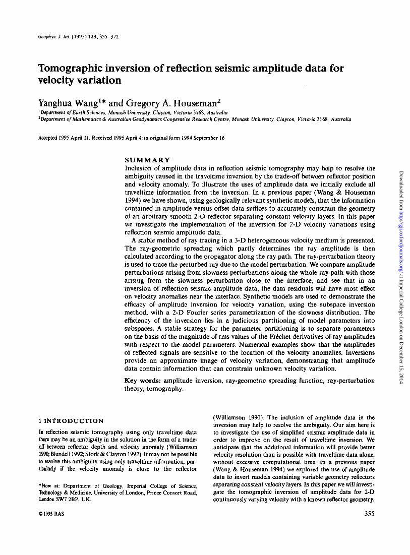
Figure 3. Inversion example 11: (a) the synthetic model with 1-D velocity variation in a horizontal direction; and the inversion solutions after (b) five iterations and (c) 50 iterations.

we write

To obtain the ‘two-point’ perturbed ray, we may now reset the initial condition AyT(ao) = [Ax(ao), Ap(ao)] in eq. (19) to

where the 3 x 3 matrix Q2 is the submatrix of the propagator calculated from eq. (23) for the perturbed central ray I * .

Once the ‘two-point’ perturbed ray trajectory 1 has been obtained, the perturbed propagator matrix n(a, a,) can be evaluated by numerical integration along the ray path. Modified ray-geometric spreading D (eq. 11) and reflection/ transmission coefficients C, and then the perturbed amplitude (eq. 16) along this ‘two-point’ perturbed ray can be determined as described above for the reference rays. The Frechet derivative


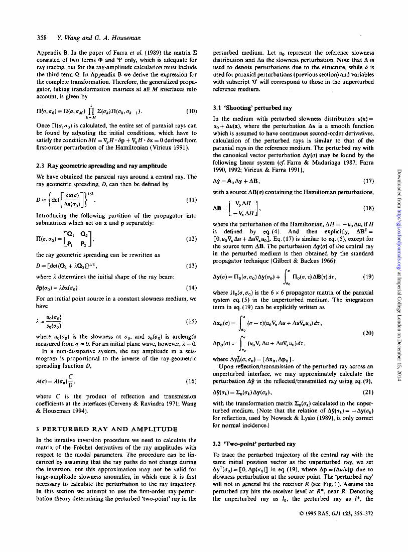
Figure4. Inversion example 12: (a) the synthetic model with 1-D velocity variation in a vertical direction; and the inversion solutions after (b) five iterations and (c) 50 iterations.

is then calculated, using the finite-difference method, from the difference between perturbed and unperturbed ray amplitudes.

4 DEPENDENCE OF AMPLITUDE ON SLOWNESS PERTURBATION

4.1 Linearized approximation of amplitude ia a simple example

Before undertaking amplitude inversion for velocity variation, we first investigate the dependence of amplitude on the perturbations to the slowness field, so as to have some insight into how the inversion procedure is affected by the reflection configuration. In our tests of amplitude inversion, we use log,, of the vertical component of displacement amplitude at the surface recorder. The perturbation of ray amplitude (under logarithm) due to the model perturbation, according to eq. (16),

0 1995 RAS, G J i 123, 355-372

at Imperial C

ollege London on D

ecember 15, 2014


ownloaded from


Inversion of rejection seismic amplitude data 361

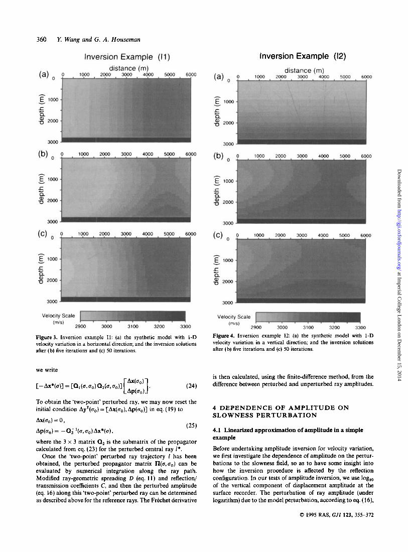
Figure 5. Inversion example I 3 (a) the synthetic model with 1-D velocity variation and a high wavenumber component (0.7km-') in a horizontal direction; and the inversion solutions after (b) five iterations and (c) 50 iterations.

can be expressed as

in terms of the ray-geometric spreading function D and the product of reflection/transmission coefficients C, where variables with subscripts '0' correspond to those in the unperturbed reference medium.

In Appendix C we use a linearized approximation for the amplitude perturbation in a simple example to derive the following approximate formulae. For the simple case of a model with constant slowness distribution (the initial estimate we used in the following inversions), the following linearized approximation of loglo(Do/D) can be obtained (see eq. (CS) in Appendix C),

h310 e A471 d r , log'' (2) zz uO(7) + Au(T)

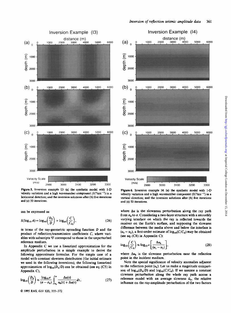
Figure6. Inversion example I 4 (a) the synthetic model with I-D velocity variation and a high wavenumber component (0.7 km-') in a vertical direction; and the inversion solutions after (b) five iterations and (c) 50 iterations.

where Au is the slownesss perturbation along the ray path from CT, to CT. Considering a two-layer structure with a smoothly varying interface on which the ray is reflected towards the receiver on the Earth's surface, and supposing the slowness difference between the media above and below the interface is (ul - u2), a first-order estimate of logl,(C/Co) may be obtained (see eq. (C8) in Appendix C):

where Auk is the slowness perturbation near the reflection point in the incident medium.

Note the special significance of velocity anomalies adjacent to the reflection point (i(k). Let us make a magnitude comparison of log,,(D,/D) and logl,(C/Co). If we assume a constant slowness perturbation along the whole ray path across a reference model with an average slowness &, the relative influence on the ray-amplitude perturbation of the two factors

0 1995 RAS, GJI 123, 355-372

at Imperial C

ollege London on D

ecember 15, 2014


ownloaded from


362 Y. Wang and G . A. Houseman

Inversion Example (15) 10'

100

10-4

+ 0.04 G= v)

5 0.03 v) v)

g 0.02 8 0.01

0.00 4 I 0 10 20 30 40 50

Iterations

Figure 8. Convergence rate of amplitude inversion 15, shown by data misfit defined by eq. (31) and the rms and (absolute) maximal differences between the synthetic model and the current estimate in the inversion.

Say iio = 300ms km-', (ul - u2) = 3 ms km-', then AE,/AE2 = 1jlOO. An important conclusion that can be drawn from eq. (29) is that the perturbation of ray amplitude depends more significantly on the slowness perturbations near the reflection point. Therefore, in an inversion of reflection seismic amplitude data, the data residuals will have most effect on velocity anomalies near the reflecting interface. If one uses the common model parametrization of dividing a velocity structure into rectangular cells, one can anticipate that a straightforward inversion algorithm will cause slowness anomalies within the layer to appear concentrated in the velocity cells adjacent to the reflector.

4.2 Singular value analysis

Using the model parametrization of slowness in terms of 2-D Fourier series (eq. l), we now try to show which Fourier components of the model can be better resolved by an inversion with amplitude data. In a linearized iterative inversion procedure, the inversion problem is characterized by the Frechet matrix. Singular value analysis of the Frechet matrix is a useful measure of the sensitivity of the model response to model parameters. It has been used effectively by Bregman, Bailey & Chapman (1989) and Pratt & Chapman (19g2) to analyse the crosshole traveltime tomography problem, and by Wang & Houseman (1994) for the analysis of the reflection seismic amplitude inversion problem for interface geometry. The singular value analysis of the Frkchet matrix is also informative in

Figure 7. Inversion example 15: (a) the synthetic model with a 2-D variable slowness distribution given by harmonic functions (eq. 37); and the inversion solutions after (b) five iterations, (c) 20 iterations and (d) 50 iterations.

eqs (27) and (28) can be estimated as the case of amplitude inversion for slowness variation. In the singular value analysis, we set N = 5 in the slowness distribution (eq. l), but in the accompanying Fig. 2, we show only the 36 slowness parameters aij , for i , j = 0,1,. . . 5 (the cosine- cosine coefficients). The FrCchet derivatives are evaluated in the solution space (with a constant background slowness). The eigenvectors and associated singular values (SVs) of the Frechet

(29)

0 1995 RAS, GJI 123, 355-372

at Imperial C

ollege London on D

ecember 15, 2014


ownloaded from



Inversion Models (with different reflector depths)

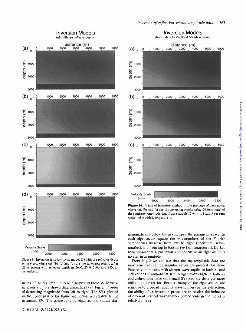
Figure 9. Inversion tests (synthetic model 15) with the reflector depth set in error, where (a), (b), (c) and (d) are the inversion results (after 20 iterations) with reflector depth at 2600, 2700, 2900 and 3000m, respectively.

matrix of the ray amplitudes with respect to these 36 slowness parameters aij are shown diagrammatically in Fig. 2, in order of decreasing magnitude from left to right. The SVs, plotted on the upper part of the figure are normalized relative to the maximum SV. The corresponding eigenvectors, shown dia-

Inversion Models (from data with 1%. 3% 8 5% white noise)

Figure 10. A test of inversion method in the presence of data noise, where (a), (b) and (c) are the inversion results (after 20 iterations) of the synthetic amplitude data from example I5 with 1, 3 and 5 per cent white noise added, respectively.

grammatically below the graph, span the parameter space. In each eigenvector square the wavenumbers of the Fourier components increase from left to right (horizontal wavenumber), and from top to bottom (vertical component). Darker tone shows that a particular component of an eigenvector is greater in magnitude.

From Fig. 2 we can see that the ray-amplitude data are most sensitive (i.e. the singular values are greatest) for those Fourier components with shorter wavelengths in both x- and z-directions. Components with longer wavelength in both x- and z-directions have only small SVs and are therefore more difficult to invert for. Because many of the eigenvectors are sensitive to a broad range of wavenumbers in the z-direction, the ability of an inversion procedure to resolve the influence of different vertical wavenumber components in the model is relatively weak.

0 1995 RAS, GJi 123, 355-372

at Imperial C

ollege London on D

ecember 15, 2014


ownloaded from



model estimate d I g(m),

F(m) = (c6 '(d - dabs), (d - dabs)) 7 (31)

where (.;) denotes the inner product and C, is the data covariance matrix. In a subspace approach, the model perturbation 6m E RM is restricted to lie in a q-dimensional subspace of RM which is spanned by the vectors {a('), j = 1, q) ,

Figure 11. Amplitude inversion example 16: (a) the synthetic model with an arbitrary localized velocity anomaly over constant background velocity distribution; and the inversion solutions after (b) five iterations and (c) 20 iterations.

5 INVERSION ALGORITHM

In the following sections we will show some examples of amplitude inversion for velocity variation assuming that the actual reflection interface is known a priori. The free parameters to be determined in the inversion are the coefficients of the basis functions (eq. l), which are referred to as the 'model' m. The dimension of the model space (allowing for the components which are zero when i = 0 or j = 0) is

M = 1 + 4 N ( N + 1 ) = 1 + 8 n . (30) N

"= 1

The inverse problem is reduced to finding a vector mERM which adequately reproduces the observations doba.

The subspace method (Kennett ef al. 1988) is used in the following examples to invert for the velocity variation. The objective function in the inversion is defined by data misfit between the observed data dobs and the forward prediction of

where A here represents the matrix of subspace vectors. The parameters clj are determined by means of minimizing a local quadratic approximation of the objective function F about some current model. The quadratic approximation implies that the perturbation of the model vector may be expressed in terms of the gradient vector of data misfit, y = V,F(m) = GTCD ' [g(m) - dabs], and the Hessian matrix, H 3 V,,,V,F(m) = GTCDIG, where G = V,g(m) is the matrix of the Frechet derivatives, as

6m= - A ( A ~ H A ) - ' A ~ ~ , (33)

(cf Kennett et al. 1988), where a minus sign indicates that the model will be updated along the steepest descent directions. Compared to the full matrix inversion, an immediate advantage of this approach is that only the q x q matrix (ATHA) needs to be inverted.

The success or failure of a subspace approach hinges upon a judicious selection of the spanning vectors for the activa- ted subspace. For the general case of M model parameters described in eq. ( l ) , we systematically allocate them into Nsub subspaces:

When N = 2, Nsub = 5. The subspaces contain respectively (and arbitrarily) 3, 4, 5, 6, 7, 8 ,... and 8 model parameters. The basis vectors {a(j)} are constructed in terms of components of the steepest ascent of data misfit corresponding to those parameters.

Although the number of subspaces and the number of parameters allocated in each subspace is a factor influencing the efficiency of the inversion (e.g. Oldenburg, McGillivray & Ellis 1993), the major factor will be how to group the parameters within each subspace. In restricting the dimension of the model space for each iteration, it may occur that vectors which are important in finding the global minimum of the desired objective function are not available and convergence to the solution is slowed or prevented. In the examples presented below, following Wang & Houseman (1994), we partition model parameters into separate subspaces on the basis of sensitivity of the amplitude data to variation of the model parameters as defined by the matrix of FrCchet derivatives. In the linearized iterative inversion, as we know, the data residual influences the update of the model parameters at a rate that depends on the sensitivity of the data to those parameters. So it is desirable to partition the model parameters into several subspaces based on the magnitude of their influence on the output data. It is rather difficult to measure the sensitivities for each model parameter individually, as seen in Fig. 2. An empirical quantity indicating the sensitivity of the amplitude with respect to a model parameter is the root-mean-squared (rms) value of the Frechet derivatives for the complete set of

0 1995 RAS, GJI 123, 355-372

at Imperial C

ollege London on D

ecember 15, 2014


ownloaded from



I

0 0.4 - -

0.2 4 I I 0 1000 2000 3000 4000 5000 6000

distance (m) . , 0 1000 2000 3000 4000 5000 6000

3200 4 I I

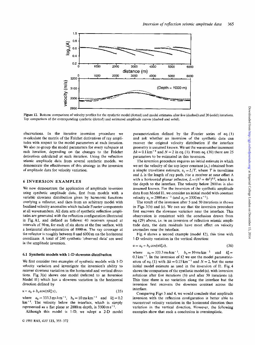
Figure 12. Bottom: comparison of velocity profiles for the synthetic model (dotted) and model estimates after five (dashed) and 20 (solid) iterations. Top: comparison of the corresponding synthetic (dotted) and estimated amplitude curves (dashed and solid).

observations. In the iterative inversion procedure we re-calculate the matrix of the Frechet derivatives of ray amplitudes with respect to the model parameters at each iteration. We also re-group the model parameters for every subspace at each iteration, depending on the changes to the FrCchet derivatives calculated at each iteration. Using the reflection seismic amplitude data from several synthetic models, we demonstrate the effectiveness of this strategy in the inversion of amplitude data for velocity variation.

6 INVERSION EXAMPLES

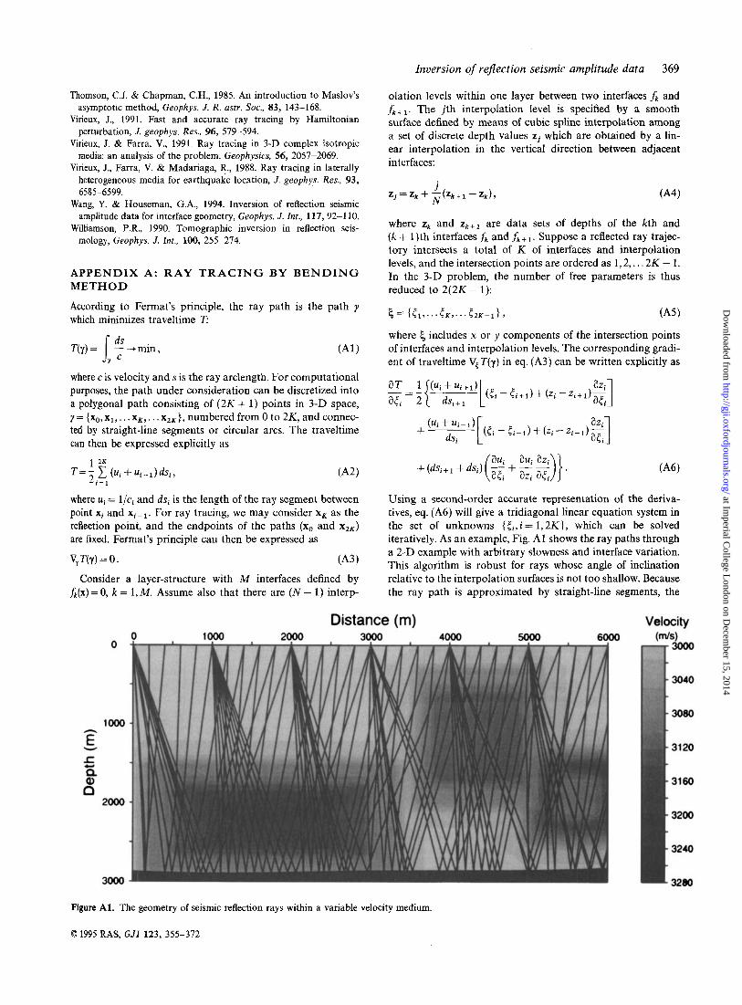
We now demonstrate the application of amplitude inversion using synthetic amplitude data, first from models with a variable slowness distribution given by harmonic functions overlying a reflector, and then from an arbitrary model with localized velocity anomalies which include Fourier components at all wavenumbers. All data sets of synthetic reflection amplitudes are generated with the reflection configuration illustrated in Fig. Al, and defined as follows: 40 receivers spaced at intervals of 50m, for each of six shots at the free surface, with a horizontal shot-separation of 1000m. The ray coverage at the reflector is roughly between 0 and 6000m on the horizontal coordinate. A total of 240 synthetic ‘observed data’ are used in the amplitude inversion.

6.1 Synthetic models with 1-D slowness distribution

We first consider two examples of synthetic models with 1-D velocity variation and investigate the inversion’s ability to recover slowness variation in the horizontal and vertical directions. Fig. 3(a) shows one model (referred to as Inversion Model 11) which has a slowness variation in the horizontal direction defined by

u=ao+b0cos(7ck$x), (35) where a, = 333.3 ms km-’, bo = lOms km-’ and k$ = 0.2 km-’. The velocity below the interface, which is simply represented as a flat plane at 2800m depth, is 3300ms-’.

Although this model is 1-D, we adopt a 2-D model

parametrization defined by the Fourier series of eq. (1) and ask whether an inversion of the synthetic data can recover the original velocity distribution if the interface geometry is assumed known. We set the wavenumber increment Ak = 0.1 km-’ and N = 2 in eq. (1). From eq. (30) there are 25 parameters to be estimated in this inversion.

The inversion procedure requires an initial estimate in which we set the velocity of the top layer constant (a1) obtained from a simple traveltime estimate, al = L/T, where T is traveltime and L is the length of ray path. For a receiver at near offset A with a horizontal planar reflector, L = (A’ + 4h’)”’, where h is the depth to the interface. The velocity below 2800m is also assumed known. For the inversion of the synthetic amplitude data from Model 11, we consider an initial model with constant velocity rxl = 2980ms-’ (and a2 = 3300ms-’).

The result of the inversion after 5 and 50 iterations is shown in Figs 3(b) and (c). We can see that the inversion procedure first recovers the slowness variation near the interface. This observation is consistent with the conclusion drawn from eq. (29) above, i.e. in an inversion of reflection seismic amplitude data, the data residuals have most effect on velocity anomalies near the interface.

Fig.4 shows a second example (model I2), this time with 1-D velocity variation in the vertical direction:

u = a. + b, cos(7c&z), (36)

where a. = 333.3 ms km-’, bo = lOms km-’ and kz, = 0.3 km-’. In the inversion of I2 we use the model parametrization of eq. (1) with Ak = 0.15 km-’ and N = 2, but the same initial model estimate as used in the inversion of 11. Fig. 4 shows the comparison of the synthetic model (a), with inversion solutions after five iterations (b) and after 50 iterations (c). This time there is no variation along the interface but the inversion first recovers the slowness contrast across the interface.

Comparing Figs 3 and 4, we would conclude that amplitude inversion with the reflection configuration is better able to reconstruct velocity variation in the horizontal direction than variation in the vertical direction. However, the following examples show that such a conclusion is oversimplistic.

0 1995 RAS, GJI 123, 355-372

at Imperial C

ollege London on D

ecember 15, 2014


ownloaded from




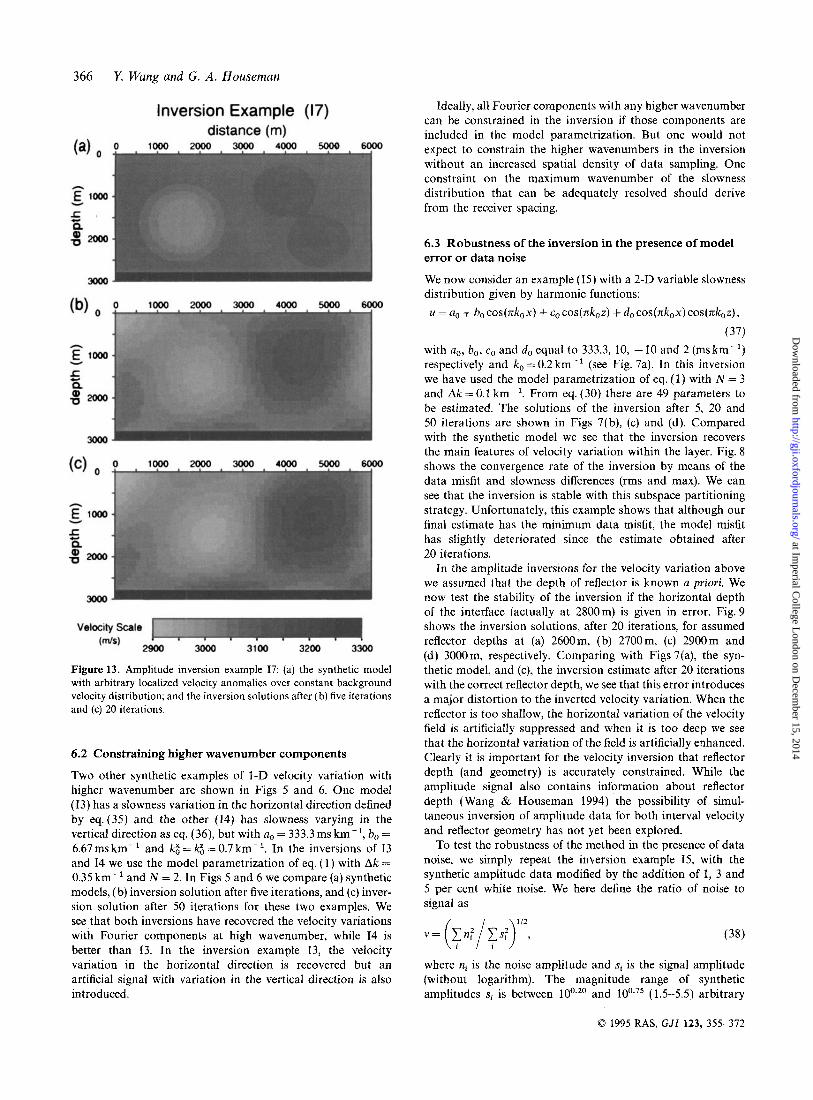
Figure 13. Amplitude inversion example 17: (a) the synthetic model with arbitrary localized velocity anomalies over constant background velocity distribution; and the inversion solutions after (b) five iterations and (c) 20 iterations.

6.2 Constraining higher wavenumber components

Two other synthetic examples of 1-D velocity variation with higher wavenumber are shown in Figs 5 and 6. One model (13) has a slowness variation in the horizontal direction defined by eq. (35) and the other (14) has slowness varying in the vertical direction as eq. (36), but with no = 333.3 ms km-', b, = 6.67mskm-' and kg = k: = 0.7km-'. In the inversions of I3 and 14 we use the model parametrization of eq. (1) with Ak = 0.35 km-' and N = 2. In Figs 5 and 6 we compare (a) synthetic models, (b) inversion solution after five iterations, and (c) inversion solution after 50 iterations for these two examples. We see that both inversions have recovered the velocity variations with Fourier components at high wavenumber, while I4 is better than 13. In the inversion example 13, the velocity variation in the horizontal direction is recovered but an artificial signal with variation in the vertical direction is also introduced.

Ideally, all Fourier components with any higher wavenumber can be constrained in the inversion if those components are included in the model parametrization. But one would not expect to constrain the higher wavenumbers in the inversion without an increased spatial density of data sampling. One constraint on the maximum wavenumber of the slowness distribution that can be adequately resolved should derive from the receiver spacing.

6.3 Robustness of the inversion in the presence of model error or data noise

We now consider an example (15) with a 2-D variable slowness distribution given by harmonic functions: u = a, + b,~~s(nk ,x) + c,co~(nk,z) + d,cos(~k,x)cos(nk,z),

(37) with a,, b,, c , and do equal to 333.3, 10, - 10 and 2 (ms km-') respectively and k , = 0.2 km-' (see Fig. 7a). In this inversion we have used the model parametrization of eq. (1) with N = 3 and Ak = 0.1 km- '. From eq. (30) there are 49 parameters to be estimated. The solutions of the inversion after 5, 20 and 50 iterations are shown in Figs 7(b), (c) and (d). Compared with the synthetic model we see that the inversion recovers the main features of velocity variation within the layer. Fig. 8 shows the convergence rate of the inversion by means of the data misfit and slowness differences (rms and max). We can see that the inversion is stable with this subspace partitioning strategy. Unfortunately, this example shows that although our final estimate has the minimum data misfit, the model misfit has slightly deteriorated since the estimate obtained after 20 iterations.

In the amplitude inversions for the velocity variation above we assumed that the depth of reflector is known a priori. We now test the stability of the inversion if the horizontal depth of the interface (actually at 2800m) is given in error. Fig. 9 shows the inversion solutions, after 20 iterations, for assumed reflector depths at (a) 2600m, (b) 2700m, (c) 2900m and (d) 3000m, respectively. Comparing with Figs 7(a), the synthetic model, and (c), the inversion estimate after 20 iterations with the correct reflector depth, we see that this error introduces a major distortion to the inverted velocity variation. When the reflector is too shallow, the horizontal variation of the velocity field is artificially suppressed and when it is too deep we see that the horizontal variation of the field is artificially enhanced. Clearly it is important for the velocity inversion that reflector depth (and geometry) is accurately constrained. While the amplitude signal also contains information about reflector depth (Wang & Houseman 1994) the possibility of simul- taneous inversion of amplitude data for both interval velocity and reflector geometry has not yet been explored.

To test the robustness of the method in the presence of data noise, we simply repeat the inversion example 15, with the synthetic amplitude data modified by the addition of 1, 3 and 5 per cent white noise. We here define the ratio of noise to signal as

v = ( i In; i i 1 s : T , (38)

where n, is the noise amplitude and si is the signal amplitude (without logarithm). The magnitude range of synthetic amplitudes si is between and (1.5-5.5) arbitrary

0 1995 RAS, GJI 123, 355-372

at Imperial C

ollege London on D

ecember 15, 2014


ownloaded from



0.6 v

0 w 0 0.4 -

0.2 4 I 0 1000 2000 3000 4000 5000 6000

distance (m) 0 1000 2000 3000 4000 5000 6000

3200 ! I I

2900 J

3200 1

............. ........ ......

3000 \ (Depth = 1600 m)

2900 J

3200 1 3100 -

3000 - (Depth = 2000 m)

Figure 14. Bottom: comparison of velocity profiles for the synthetic model (dotted) and model estimates after five (dashed) and 20 (solid) iterations, at 1200m, 1600m and 2000m. Top: comparison of the corresponding synthetic (dotted) and estimated amplitude curves (dashed and solid).

units; the amplitude range of 1, 3 or 5 per cent noise ni is kO.08, f0.2 or f0.4 in the same units (Wang & Houseman 1994). Fig. 10 shows the inversion results after 20 iterations. The amplitude inversion of the data with 1 per cent noise added (Fig. 10a) converges very well. In the inversions of data with 3 and 5 per cent noise added, although both inversions have recovered approximately the velocity distribution in the area close to the reflector, the vertical velocity variation is poorly represented in these inversion solutions. The inversion of the data with 3 per cent noise (Fig. lob) has determined the general shape of the model feature but overestimated the amplitude of variation. The inversion with 5 per cent noise (Fig. 1Oc) seems to have suppressed the vertical velocity variation.

6.4 Inversion of arbitrary smooth velocity anomalies

In the above examples (11-15) the actual solution could be represented exactly using the model parametrization. We now consider two more complex cases in which the model velocity distribution cannot be represented exactly using the model Fourier series, because it includes components at all wavenumbers, including high wavenumbers that are not represented in the model parametrization. Model I6 (Fig. l l a ) is an arbitrary model with a localized velocity anomaly. Model I6 has relatively stronger velocity gradients than the preceding models

(see profile in the bottom of Fig. 12 and note the rapid change in gradient at horizontal distance 1700 m and 4600 m), implying Fourier components at high wavenumbers.

In the inversion of amplitude data from synthetic model 16, we set Ak = 0.25 km-' and N = 2 in the Fourier series parametrization. After only five iterations the velocity anomaly has appeared approximately in the solution. Comparing Figs 11 (b) and (c), which show the inversion solutions after 5 and 20 iterations, with the synthetic model of Fig. ll(a), we see that the main anomaly is reasonably well reconstructed. Fig. 12 compares velocity profiles (at depth 1000m) and amplitude curves from the current estimate (after 5 and 20 iterations) with those from the synthetic model. The data misfit is minimum after four iterations. If the inversion iterations are continued beyond that minimum the data misfit remains at the same level. As the comparison of amplitude curves in Fig. 12 shows, there is little further improvement in the model or in the fit to the data between 5 and 20 iterations. The data misfit remains relatively large because the Fourier series parametrization cannot represent the higher wavenumbers present in the original model. However, for most purposes, the inversion illustrated in Fig. 11 would be considered a successful representation of the original model.

Finally, we show one more synthetic model with an arbitrary velocity distribution and more structure at high wavenumber. Fig. 13(a) shows a model (17) with a negative velocity anomaly

0 1995 RAS, GJI 123, 355-312

at Imperial C

ollege London on D

ecember 15, 2014


ownloaded from



and two smaller positive velocity anomalies. As for the inversion of 11, we set N = 2 and Ak = 0.25 km-'. The inversion solutions after 5 and 20 iterations are shown in Figs 13(b) and (c). Comparing the inversion models with the synthetic model, we see that the main anomaly is approximately resolved, but the inversion failed to separate the two smaller positive velocity anomalies. Consistent with Fig. 2, the Fourier components in z-direction are poorly resolved. Fig. 14 shows the velocity profiles a t depths 1200m, 1600m and 2000m and the Lorresponding amplitude curves. We conclude from these two last examples that the inversion method is stable when a high wavenumber structure is present, and even if this structure remains unresolved, the solution provides a reasonable smoothed approximation to the actual structure.

7 CONCLUSIONS

We have demonstrated the inversion of amplitude data to estimate velocity variation in 2-D structures. Although the problem is relatively poorly constrained due to the reflection configuration, we have still obtained some quite encouraging results using a 2-D Fourier series model parametrization of the slowness distribution instead of the commonly used cellular parametrization. Certainly, the choice of the number of terms in the 2-D Fourier series and the fundamental wavenumber Ak are important factors influencing the inversion processing which need further study. In this work we have focused primarily on establishing that reflection seismogram amplitudes contain sufficient information to permit inversion for an unknown velocity distribution. Because of the limitation of computer resources, only problems with a relatively small number of degrees of freedom are tested here, and a n important goal for further work is to speed up the calculation of Frechet derivatives. The perturbation approach we use is quite stable for the calculation of amplitude perturbation.

In the inversion we use the subspace method, which is ideally suited for the large-scale inverse problem. We partition model parameters into separate subspaces on the basis of sensitivity of the amplitude response with respect to model parameters (the coefficients of 2-D Fourier series). The inversion converges stably in the case of models with smoothly varying velocity and velocity gradient. Even where the model velocity cannot be exactly represented by the inversion parametrization, the long-wavelength components of the model are satisfactorily recovered. The relatively less successful behaviour of the inversion in the presence of data noise, or in the case of systematic errors in the reflector geometry, may indicate sig- nificant limitations on the use of amplitude data in tomographic inversion. Nevertheless, the amplitudes of the reflected signals are sensitive to the location of the velocity anomalies and the inversions provide an approximate image of velocity variation, thus demonstrating that amplitude data contain information that can constrain unknown velocity variation. Further work should use amplitude data in conjunction with traveltime data from reflection seismograms to better constrain subsurface velocity distribution.

ACKNOWLEDGMENTS

We thank an anonymous reviewer for comments which resulted in improvements to the text. Y W s research was partially

supported by a scholarship from the Australian Geodynamics CRC during 1994.

REFERENCES

Aki, K. & Richards, P., 1980. Quantitative Seismology: Theory and Method, W. H. Freeman, San Francisco.

Blundell, C.A., 1992. Illustrating the trade-off between velocity and reflector position in travel-time inversion by using a two-dimensional subspace, Expl. Geophys., 23( 1/2), 27-32.

Bregman, N.D., Bailey, R.C. & Chapman, C.H., 1989. Ghosts in tomography: the effects of poor angular coverage in 2-D seismic traveltime inversion, Can. J . expl. Geophys., 25, 7-27.

Burridge, R., 1976. Some Mathematical Topics in Seismology, Courant Institute of Mathematical Sciences, New York University, New York.

Cerveny, V., 1985. The application of ray tracing to numerical modelling of seismic wave fields in complex structures, in Handbook of Geophysical Exploration, Section I , Seismic Exploration, Vol. 15A, pp. 1-119, Geophysical Press, London.

Cerveny, V. & Ravindra, R., 1971. Theory of Seismic Head Waves, University of Toronto Press.

Cerveny, V., Molotkov, LA. & Psencik, I., 1977. Ray Method in Seismology, University Karlova, Praha.

Chapman, C.H., 1985. Ray theory and its extensions: WKBJ and Maslov seismograms, J . Geophys., 58, 27-43.

Farra, V., 1990. Amplitude computation in heterogeneous media by ray perturbation theory: A finite element approach, Geophys. J . Int., 103, 341-354.

Farra, V., 1992. Bending method revisited a Hamiltonian approach, Geophys. J . Int., 109, 138-150.

Farra, V. & Madariaga, R., 1987. Seismic waveform modelling in heterogeneous media by ray perturbation theory, J. geophys. Res.,

Farra, V., Virieux, J. & Madariaga, R., 1989. Ray perturbation theory for interfaces, Geophys. J . Int., 99, 377-390.

Gilbert, F. & Backus, G.E., 1966. Propagator matrices in elastic wave and vibration problems, Geophysics, 31, 326-333.

Kendall, J.-M. & Thomson, C.J., 1989. A comment on the form of the geometrical spreading equations, with some numerical examples of seismic ray tracing in inhomogeneous, anisotropic media, Geophys. J . Int., 99, 401-413.

Kennett, B.L.N., Sambridge, M.S. & Williamson, P.R., 1988. Subspace methods for large inverse problems with multiple parameter classes, Geophys. J., 94, 237-247.

MacDonald, C., Davis, P.M. & Jackson, D.D., 1987. Inversion of reflection travel times and amplitudes, Geophysics, 52, 606-61 7.

Moser, T.J., Nolet, G. & Snieder, R., 1992. Ray bending revisited, Bull. seism. SOC. Am., 82, 259-288.

Nowack, R.L. & Lutter, W.J., 1988. Linearized rays, amplitude and inversion, Pure appl. Geophys., 128, 401-421.

Nowack, R.L. & Lyslo, J.A., 1989. Frechet derivatives for curved interfaces in the ray approximation, Geophys. J., 97, 497-509.

Oldenburg, D.W., McGillivray, P.R. & Ellis, R.G., 1993. Generalized subspace methods for large-scale inverse problems, Geophys. J . Int.,

Pratt, R.G. & Chapman, C.H., 1992. Traveltime tomography in anisotropic media-11. Application, Geophys. J. Int., 109, 20-37.

Sambridge, M.S., 1990. Non-linear arrival time inversion: constraining velocity anomalies by seeking smooth models in 3-D, Geophys. J . Int., 102, 653-677.

Stork, C. & Clayton, R.W., 1992. Using constraints to address the instabilities of automated prestack velocity analysis, Geophysics,

Thomson, C.J., 1983. Ray-theoretical amplitude inversion for laterally varying velocity structure below NORSAR, Geophys. J . R . astr. SOC.,

92, 2697-2712.

114, 12-20.

57,404-419.

74, 525-558.

0 1995 RAS, GJI 123, 355-312

at Imperial C

ollege London on D

ecember 15, 2014


ownloaded from



Thomson, C.J. & Chapman, C.H., 1985. An introduction to Maslov’s asymptotic method, Geophys. J. R. astr. Soc., 83, 143-168.

Virieux, J., 1991. Fast and accurate ray tracing by Hamiltonian perturbation, J. geophys. Rex, 96, 579-594.

Virieux, J. & Farra, V., 1991. Ray tracing in 3-D complex isotropic media: an analysis of the problem, Geophysics, 56, 2057-2069.

Virieux, J., Farra, V. & Madariaga, R., 1988. Ray tracing in laterally heterogeneous media for earthquake location, J. geophys. Res., 93,

Wang, Y. & Houseman, G.A., 1994. Inversion of reflection seismic amplitude data for interface geometry, Geophys. J. Int., 117, 92-110.

Williamson, P.R., 1990. Tomographic inversion in reflection seismology, Geophys. J . Int., 100, 255-274.

6585-6599.

APPENDIX A: RAY TRACING BY BENDING METHOD

According to Fermat’s principle, the ray path is the path y which minimizes traveltime T

where cis velocity and s is the ray arclength. For computational purposes, the path under consideration can be discretized into a polygonal path consisting of (2K + 1 ) points in 3-D space, y = {xo,xl,. . . x K , . . . x,,}, numbered from 0 to 2K, and connec- ted by straight-line segments or circular arcs. The traveltime can then be expressed explicitly as

I 2K T = - C ( ~i +u;-1)dsi, “42)

2,,1

where ui = l/ci and dsi is the length of the ray segment between point xi and xi - 1 . For ray tracing, we may consider x K as the reflection point, and the endpoints of the paths (xo and XZK)

are fixed. Fermat’s principle can then be expressed as

V,T(y)=O. (A3 1 Consider a layer-structure with M interfaces defined by

fk (x) = 0, k = 1, M . Assume also that there are ( N - 1) interp-

olation levels within one layer between two interfaces f k and f k + l . The jth interpolation level is specified by a smooth surface defined by means of cubic spline interpolation among a set of discrete depth values zj which are obtained by a linear interpolation in the vertical direction between adjacent interfaces:

where zk and zk+l are data sets of depths of the kth and ( k + 1)th interfaces fk and fk+l. Suppose a reflected ray trajectory intersects a total of K of interfaces and interpolation levels, and the intersection points are ordered as 1,2,. . .2K - 1. In the 3-D problem, the number of free parameters is thus reduced to 2(2K - 1):

where 6 includes x or y components of the intersection points of interfaces and interpolation levels. The corresponding gradient of traveltime V,T(y) in eq. (A3) can be written explicitly as

Using a second-order accurate representation of the derivatives, eq. (A6) will give a tridiagonal linear equation system in the set of unknowns (&,i = 1,2K}, which can be solved iteratively. As an example, Fig. A1 shows the ray paths through a 2-D example with arbitrary slowness and interface variation. This algorithm is robust for rays whose angle of inclination relative to the interpolation surfaces is not too shallow. Because the ray path is approximated by straight-line segments, the

Figure Al . The geometry of seismic reflection rays within a variable velocity medium.

0 1995 RAS, G J I 123, 355-372

at Imperial C

ollege London on D

ecember 15, 2014


ownloaded from



algorithm should not be expected to give accurate results in the vicinity of turning rays.

APPENDIX B: REFLECTION A N D TRANSMISSION O N CURVED INTERFACE

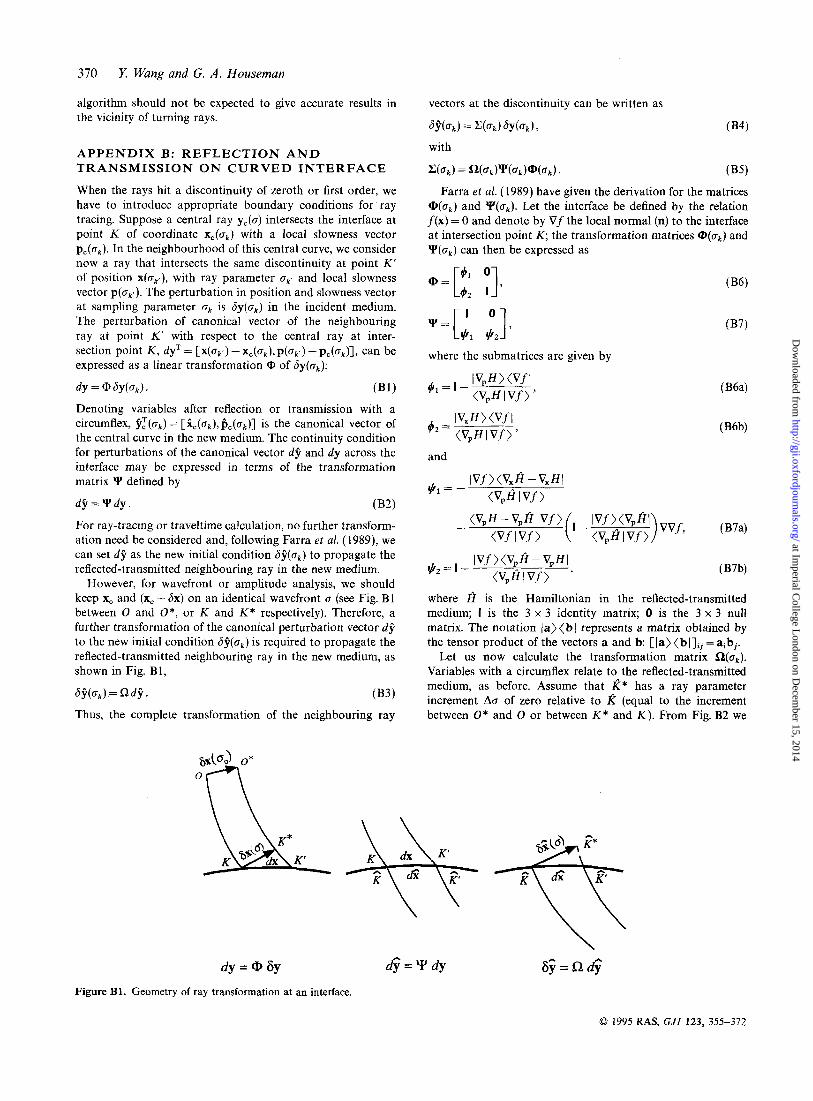
When the rays hit a discontinuity of zeroth or first order, we have to introduce appropriate boundary conditions for ray tracing. Suppose a central ray y,(a) intersects the interface at point K of coordinate x,(ak) with a local slowness vector &(a,). In the neighbourhood of this central curve, we consider now a ray that intersects the same discontinuity at point K' of position x(akr), with ray parameter ok' and local slowness vector P((Tk'). The perturbation in position and slowness vector at sampling parameter ak is 6y(ak) in the incident medium. The perturbation of canonical vector of the neighbouring ray at point K' with respect to the central ray at intersection point K , dy' = [x(gk') - xc(ak), p(a,,) - pC(ak)], can be expressed as a linear transformation @ of 6y(ok):

dy = @ 6y(ak). (B1) Denoting variables after reflection or transmission with a circumflex, f;(ak) = [j;,(ak),fi,(ak)] is the canonical vector of the central curve in the new medium. The continuity condition for perturbations of the canonical vector df and dy across the interface may be expressed in terms of the transformation matrix Y defined by

df = Y dy . (B2)

For ray-tracing or traveltime calculation, no further transformation need be considered and, following Farra et al. (1989), we can set df as the new initial condition 6f(ak) to propagate the reflected-transmitted neighbouring ray in the new medium.

However, for wavefront or amplitude analysis, we should keep x, and (x, + 6x) on an identical wavefront a (see Fig. B1 between 0 and 0*, or K and K* respectively). Therefore, a further transformation of the canonical perturbation vector df to the new initial condition 6f(ak) is required to propagate the reflected-transmitted neighbouring ray in the new medium, as shown in Fig. B1,

6f(ak) = C2 df . (B3) Thus, the complete transformation of the neighbouring ray

vectors at the discontinuity can be written as

6 f ( a k ) z:(ak) 6y(ak) 9 034)

z(ak) = o(ak)y(ak)@(ak). (B5)

with

Farra et al. (1989) have given the derivation for the matrices @(a,) and y(ak). Let the interface be defined by the relation f(x) = 0 and denote by Vf the local normal (n) to the interface at intersection point K; the transformation matrices @(ak) and y(ak) can then be expressed as

where the submatrices are given by

and

where H is the Hamiltonian in the reflected-transmitted medium; I is the 3 x 3 identity matrix; 0 is the 3 x 3 null matrix. The notation la)(bl represents a matrix obtained by the tensor product of the vectors a and b: [la)(bllij=aibj.

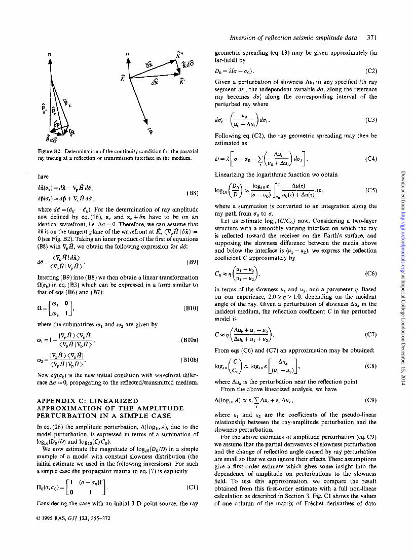
Let us now calculate the transformation matrix f2(ok). Variables with a circumflex relate to the reflected-transmitted medium, as before. Assume that K* has a ray parameter increment Aa of zero relative to K (equal to the increment between O* and 0 or between K * and K). From Fig. B2 we

dy = CP Sy

Figure B1. Geometry of ray transformation at an interface.

d: = Y dy i5i = SZ dq

0 1995 RAS, GJI 123, 355-372

at Imperial C

ollege London on D

ecember 15, 2014


ownloaded from



n

9

Figure B2. Determination of the continuity condition for the paraxial ray tracing at a reflection or transmission interface in the medium.

have

&%(u,) = d% - VpHd6,

h f i ( ~ , ) = dfi + VxHd6,

where d6 = ( 6 k ' - 6,). For the determination of ray amplitude now defined by eq.(16), x, and x,+6x have to be on an identical wavefront, i.e. Aa = 0. Therefore, we can assume that 6% is on the tangent plane of the wavefront at K, (VpH 16%) = 0 (see Fig. B2). Taking an inner product of the first of equations (B8) with VPA, we obtain the following expression for d6:

(VpH 1 an) (VPH I VPH).

dB =

Inserting (B9) into (B8) we then obtain a linear transformation Q(a,) in eq. (B3) which can be expressed in a form similar to that of eqs (B6) and (B7):

where the submatrices w1 and w2 are given by

(BlOa)

(Blob)

Now 6y(a,) is the new initial condition with wavefront difference Ao = 0, propagating to the reflected/transmitted medium.

APPENDIX C: LINEARIZED APPROXIMATION OF THE AMPLITUDE PERTURBATION I N A SIMPLE CASE

In eq. (26) the amplitude perturbation, A( log,, A), due to the model perturbation, is expressed in terms of a summation of

We now estimate the magnitude of log,,(D,/D) in a simple example of a model with constant slowness distribution (the initial estimate we used in the following inversions). For such a simple case the propagator matrix in eq. (7) is explicitly

~0g10(~,/f)) and log10(C/~o).

I (o-ao)l no(a,oo)= [() , 1. Considering the case with an initial 3-D point source, the ray

geometric spreading (eq. 13) may be given approximately (in far-field) by

Do=L(a-ao). (C2) Given a perturbation of slowness Aui in any specified ith ray segment ds,, the independent variable dui along the reference ray becomes d 4 along the corresponding interval of the perturbed ray where

Following eq. (C2), the ray geometric spreading may then be estimated as

D = L [a - a. - $. ("-) u, + Aui dai]

Linearizing the logarithmic function we obtain

log10 e dt, loglo (%) %

uo(z) + Au(z)

where a summation is converted to an integration along the ray path from oo to a.

Let us estimate logl,(C/Co) now. Considering a two-layer structure with a smoothly varying interface on which the ray is reflected toward the receiver on the Earth's surface, and supposing the slowness difference between the media above and below the interface is (u, - u2), we express the reflection coefficient C approximately by

in terms of the slowness u, and u2, and a parameter q. Based on our experience, 2.0 2 q 2 1.0, depending on the incident angle of the ray. Given a perturbation of slowness Auk in the incident medium, the reflection coefficient C in the perturbed model is

From eqs (C6) and (C7) an approximation may be obtained:

where Auk is the perturbation near the reflection point. From the above linearized analysis, we have

A( log10 A) % ~11 Aui + ~2 Auk, L

where E , and E~ are the coefficients of the pseudo-linear relationship between the ray-amplitude perturbation and the slowness perturbation.

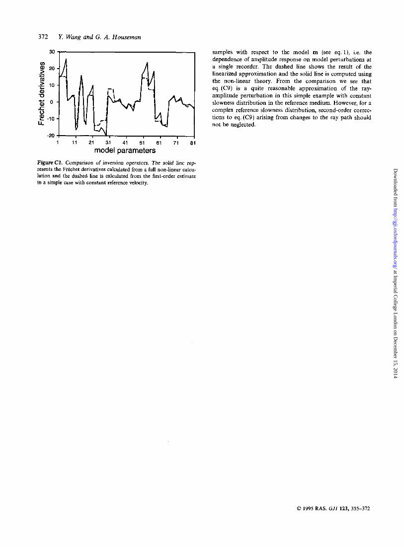
For the above estimates of amplitude perturbation (eq. C9) we assume that the partial derivatives of slowness perturbation and the change of reflection angle caused by ray perturbation are small so that we can ignore their effects. These assumptions give a first-order estimate which gives some insight into the dependence of amplitude on perturbations to the slowness field. To test this approximation, we compare the result obtained from this first-order estimate with a full non-linear calculation as described in Section 3. Fig. C1 shows the values of one column of the matrix of Frechet derivatives of data

0 1995 RAS, GJI 123, 355-372

at Imperial C

ollege London on D

ecember 15, 2014


ownloaded from


372 Y. Wang and G. A. Housevnan

30 , i

1 11 21 31 41 51 61 71 81

model parameters Figure C1. Comparison of inversion operators. The solid line represents the Frechet derivatives calculated from a full non-linear calculation and the dashed line is calculated from the first-order estimate in a simple case with constant reference velocity.

samples with respect to the model m (see eq. l), i.e. the dependence of amplitude response on model perturbations at a single recorder. The dashed line shows the result of the linearized approximation and the solid line is computed using the non-linear theory. From the comparison we see that eq.(C9) is a quite reasonable approximation of the ray- amplitude perturbation in this simple example with constant slowness distribution in the reference medium. However, for a complex reference slowness distribution, second-order correc- tions to eq. (C9) arising from changes to the ray path should not be neglected.

0 1995 RAS, GJI 123, 355-372

at Imperial C

ollege London on D

ecember 15, 2014


ownloaded from


tomographic inversion of reflection seismic amplitude … · · 2016-04-20tomographic inversion...

Documents