us000009296474b120160329 - nasa · us 9,296,474 b1 page 2 (56) references cited other publications...

11111111111111111111111111111111111111111111111111111111111111111111

(12) United States Patent Nguyen et al.

(54) CONTROL SYSTEMS WITH NORMALIZED AND COVARIANCE ADAPTATION BY OPTIMAL CONTROL MODIFICATION

(71) Applicant: The United States of America as Represented by the Administrator of the National Aeronautics & Space Administration (NASA), Washington, DC (US)

(72) Inventors: Nhan T. Nguyen, Santa Clara, CA (US); John J. Burken, Tehachapi, CA (US); Curtis E. Hanson, Lancaster, CA (US)

(73) Assignee: The United States of America as Represented by the Administrator of the National Aeronautics & Space Administration (NASA), Washington, DC (US)

(*) Notice: Subject to any disclaimer, the term of this patent is extended or adjusted under 35 U.S.C. 154(b) by 376 days.

(21) Appl. No.: 13/956,736

(22) Filed: Aug. 1, 2013

Related U.S. Application Data

(60) Provisional application No. 61/798,236, filed on Mar. 15, 2013, provisional application No. 61/679,945, filed on Aug. 6, 2012.

(51) Int. Cl. G05B 13104 (2006.01) H03H 21100 (2006.01) B64C19100 (2006.01)

(52) U.S. Cl. CPC .............. B64C 19100 (2013.01); G05B 131048

(2013.01) (58) Field of Classification Search

CPC ............... G05B 19/41835; G05B 2219/41232; G05B 2219/41217; G05B 13/027; H03H

21/0021 See application file for complete search history.

(1o) Patent No.: US 9,296,474 B1 (45) Date of Patent: Mar. 29, 2016

(56) References Cited

U.S. PATENT DOCUMENTS

8,285,659 131 * 10/2012 Kulkarni ................ G05B 17/02 244/76 R

8,489,528 132 * 7/2013 Chowdhary ............. G06N 3/08 706/21

2004/0176860 Al* 9/2004 Hovakimyan ......... G05B 13/02 700/29

2006/0217819 Al* 9/2006 Cao ...................... G05B 13/027 700/28

2010/0030716 Al* 2/2010 Calise .................. G05B 13/027 706/23

20 10/03 123 65 Al* 12/2010 Levin ............... G05B 19AI835 700/37

OTHER PUBLICATIONS

Nguyen, et al., An Optimal Control Modification to Mode .... Proceeds of AIAA Guidance, Navigation and Control Conference and Exhibit, Aug. 18-21, 2008, Honolulu, Hawaii.

(Continued)

Primary Examiner Kenneth M Lo Assistant Examiner Sunray R Chang (74) Attorney, Agent, or Firm Christopher J. Menke; Robert M. Padilla; John F. Schipper

(57) ABSTRACT

Disclosed is a novel adaptive control method and system called optimal control modification with normalization and covariance adjustment. The invention addresses specifically to current challenges with adaptive control in these areas: 1) persistent excitation, 2) complex nonlinear input-output map-ping, 3) large inputs and persistent learning, and 4) the lack of stability analysis tools for certification. The invention has been subject to many simulations and flight testing. The results substantiate the effectiveness of the invention and demonstrate the technical feasibility for use in modern air-craft flight control systems.

18 Claims, 35 Drawing Sheets

F:aferenxe Model

110 105 r

.. --- - _

Certiuller ' Uncr~rtaio Plant-----

~

I / e

120 150 155 160 1 70

optimal Control j

1 fviodific~tion

AdWi 3.;n Pl -olization _ F•

205

Adaptive Control Sya*.arn

100

A6pbn Control System wi?h Optimal Mudification (Adaptive iaw and

Adaptive Gan: Poorn:aGzztn;n Met:Lai

https://ntrs.nasa.gov/search.jsp?R=20160004241 2018-06-14T06:50:38+00:00Z

US 9,296,474 B1

(56) References Cited

OTHER PUBLICATIONS

Nguyen, Robust Optimal Adaptive Control Method with Large Adap-tive Gain, Proceeds of AIAA Infotech@Aerospace Conference, Apr. 6-9, 2009, Seattle, Washington. Nguyen, et al., Optimal Control Modification for Robust Adaptation of Singula .... AIAA Guidance, Navigation, and Control Confer-ence, Aug. 10-13, 2009, Chicago, Illinois. Nguyen, Advances in Adaptive Control Methods, NASA Aviation Safety Technical Conference, Nov. 17-19, 2009, McLean, Virginia. Nguyen, Asymptotic Linearity of Optimal Control Modification Adaptive Law with Analytical Sta . . . , Proceeds of AIAA Infotech@Aerospace, Apr. 20-22, 2010, Atlanta, Georgia.

Burken, et al., Adaptive Flight Control Design with Optimal Control Modification on an F-18 Aircraft Model, AIAA Infotech@ Aero-space, Apr. 20-22, 2010, Atlanta, Georgia. Nguyen, Optimal Control Modification Adaptive Law for Time-Scale Separated Systems, NASA Publications, Jun. 30, 2010. Nguyen, Verifiable Adaptive Control with Analytical Stability Mar-gins by Optimal Control Modification, AIAA, Aug. 2, 2010. Campbell, et al., An Adaptive Control Simulation Study using Pilot Handl .... AIAA Guidance, Navigation, and Control Conference, Aug. 2-5, 2010, Toronto, Ontario, Canada. Hanson, et al., Handling Qualities Evaluations for Low Complexity Model Reference Adaptive Controllers for Reduced Pitch and Roll Damping Scenarios, AIAA, Jul. 18, 2011.

* cited by examiner

U.S. Patent Mar. 29, 2016 Sheet 1 of 35 US 9 ,296,474 B1

115

Deference Model

110 i4 105 1 1

Ada pi~ia ~ roll~r

--------------

i"

120

Uncertain Plant fir,

('I

(7

Optimal Control Modification

Adaptive Control System 100

Fig. 1- Ada ptive Control System with Optimal Control Modification Adaptive Law

U.S. Patent Mar. 29, 2016 Sheet 2 of 35 US 9,296,474 BI

Model, Reference

------------------------- 135

Feedback Controller

1 , 4- , 0

-

-

------------------------------

Cont;oller Atreraft ---------------------

130

Adapt ~ve Opt. Controllel - LIJf

155, 160

Fig. 2 - Adaptive Flight Control Architecture

145

U.S. Patent Mar. 29, 2016 Sheet 3 of 35 US 9,296,474 B1

Fig. 3 - NASA F/A-18 Research Test Aircraft Tail Number 853


t q Adop

n 7777777777777-

{, s

Fig. 4 - Time History of Longitudinal States due to are A-Matrix Failure (C, Shift at 13 sec) with and without Optimal Control Modification Adaptive Law 150


{< a'

x {S

_01.3_IIIIJ -----------------------1----------------------- L----- -------- -------- . 3------ -------- ----------------------------- --------------

yr

{ Ad,

tics .i

Fig. 5 - Tiine History of Tracking Errors due to are A-Matrix Failure (C,., « Shift at 13 sec) with and without Optimal Control Modification Adaptive Law 150


:A ap A.

,k

Y~J

:y?

;.s

15

y

tz

r?

TW3' zz ,

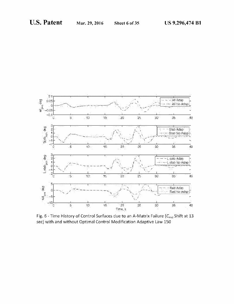
Fig. 6 - Time History of Control Surfaces due to an A-Matrix Failure (C,,,, Shift at 13 sec) with and without Optimal Control Modification Adaptive Law 150


j 3w

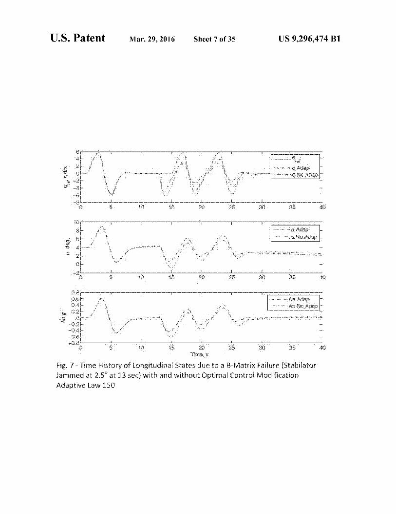
Fig. 7 - Time History of Longitudinal States due to a B-Matrix Failure (Stabilator Jammed at 2;5" at 1.3 sec) with and without Optimal Control Modification Adaptive Law 150


n

1

Y' Sv

`: f do

............................................. .... .... ... :....

L:uc

h

N,—s ' dap

_x

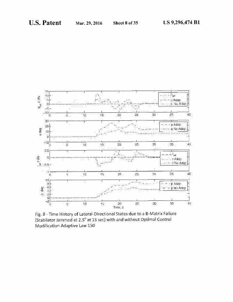
Fig. 8 - Time History of Lateral -Directional States clue to e B-matrix Failure (Stabilator Jammed at 2.5' at 13 sec) with and without Optimal Control Modification Adaptive Law 150


f• '%

`> N' #'SQL£

_ k

~rNi 4'.ie....

ap -v .a

t

A f ~$

l!

1

55

T'.'r,

k. S {e

~y

`---- ------------------- ----------------------- t----------------------- L -- - 1 ----------------------- i----------------------- - - --- '

Fig. 9 - Time history of Tracking Errors due to a B-Matrix Failure (5tabilator Jammed at 2.5 ° at 1.3 sec) with and without Optimal Control Modification Adaptive Lave 150


15

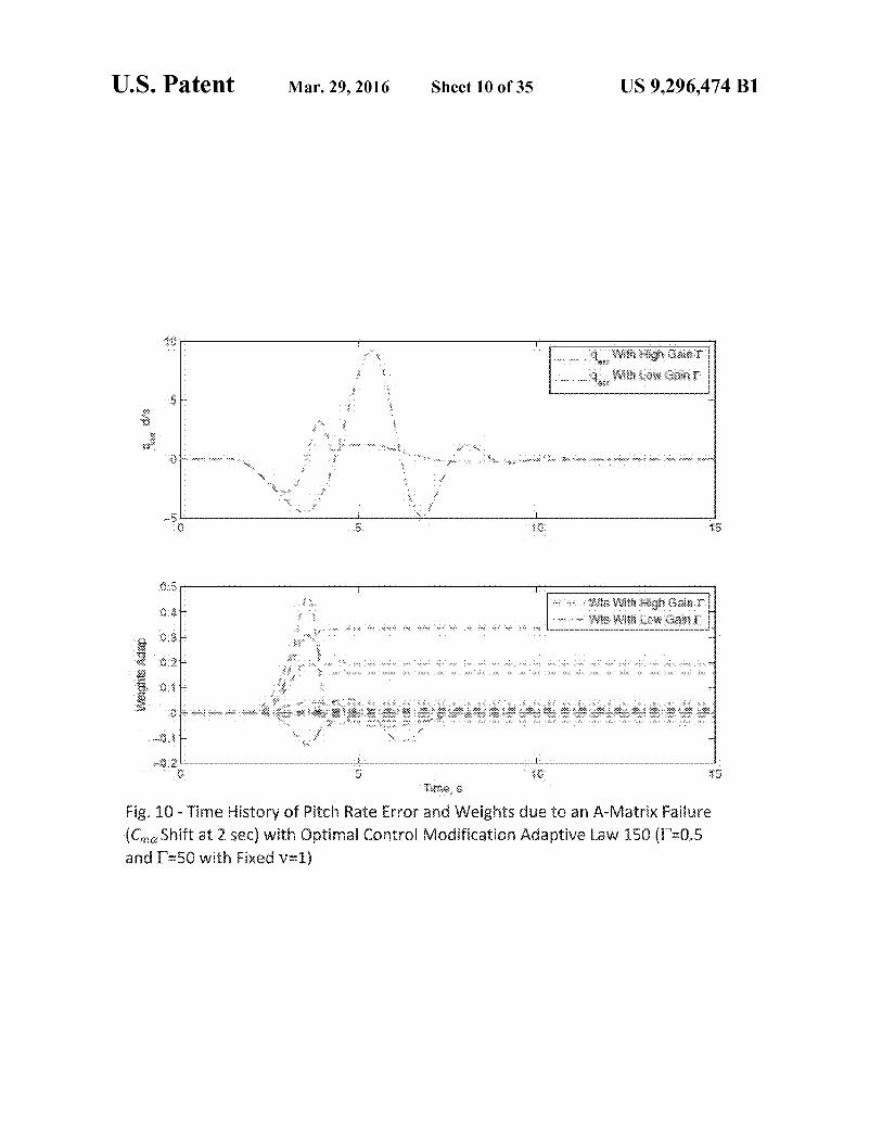
Fig. 1U- Time History of Pitch Rate Error and Weights due to an ArK8atriX Failure (Cno ShUta1Z sec) with Optimal Control Modification Adaptive Law 250(l`=[L5 and T-=5O with Fixed v=l\


r: -------- -------- -------- ---------r ------- ------ ------ ------ -------- -------- -------- --------- 140 ,,

ti

} fl

a

~ s, . ,........~..:.. _......~.~::n::.wc8 c•. xV :,:aa _:...wx.~..a .N.v-.{.:; . -cw.~y..,ax,......,.>.... `::. ..

t}

Tim* ,

Fig. 11 -Time History of Pitch Date Error and Tights due to an A-Matrix Failure (C,a Shift at 2 sec) with Optimal Control Modification Adaptive Law 150 (Fixed I-`=5 with v=0.25 and v=1)


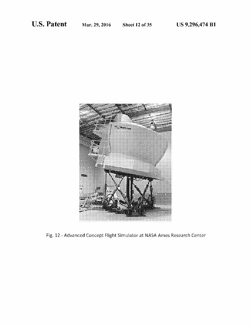
Fie. 12 - Advanced Concept Flight Simulator at NASA Ames Research Center

z


Onv63w

AIWI..c O k7NINIM*.i: PIRI'P."

C-UnImAz'r

iS

ti

Fig. 13 - Pilot Cooper-Harper Ratings of Adaptive Flight Controllers in Advanced Concept Flight Simulator

5 10 t

U.S. Patent Mar. 29, 2016 Sheet 14 of 35

US 9,296,474 B1

2

0''`

1.5

0.5

0

0 5 10 0 5 10 t t

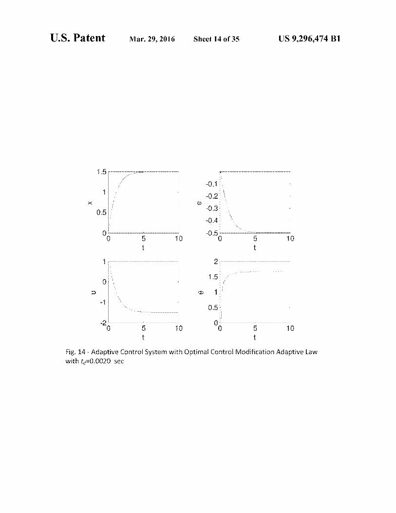
Fig. 14 - Adaptive Control System with Optimal Control Modification Adaptive Law with t,1=0.0020 sec

0 5 t

10

5 1

5 10

t


US 9,296,474 BI

4---

3

2

0

5

0

-5

1 0

0

0 5 10 0 5 10

t t

Fig. 15 - Adaptive Control System with Optimal Control Modification Adaptive Law

with td=0.2795 sec

2

1,5

0.5 Fief. Mode

0 5 t

10

3 3

2

1

0 0 5 10 0 5 10

t t

Fig. 16 - Scaled Input-Output Property of Adaptive Control



US 9,296,474 B1

5

0

v5

0

100

50

0

-50

-100 10 20 0 10 20

t t

0

20

_5 15

10

10 5

15 c 0 10 20 0 10

t

Fig. 17 - Instability of MRAC by Rohrs Counterexample

U. S . Patent

Mar. 29, 2016 Sheet 18 of 35 US 9,296,474 BI

25

20

15

= 1U 2

5

O 0 0.1 O ~ 2 0,304 &5 M 0.7 0.8 0.9 1

100

50 ___--'---

41-

| '

-50 1 0 11 C2 03 04 O5 0.8 0.7 0.8 0.9 1

V

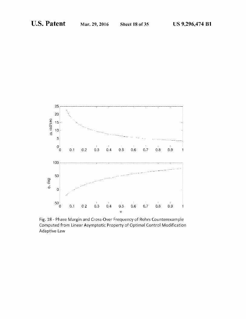
Fig. 18 Phase Margin andCrosu-OverFrequencyofRohrs[ounterexarnp|e Computed from Linear Asymptotic Property of Optimal Control Modification Adaptive Law

U.S. Patent Mar. 29, 2016

Sheet 19 of 35

US 9,296,474 BI

4. ..........

2

,2

4

2 4

6 f

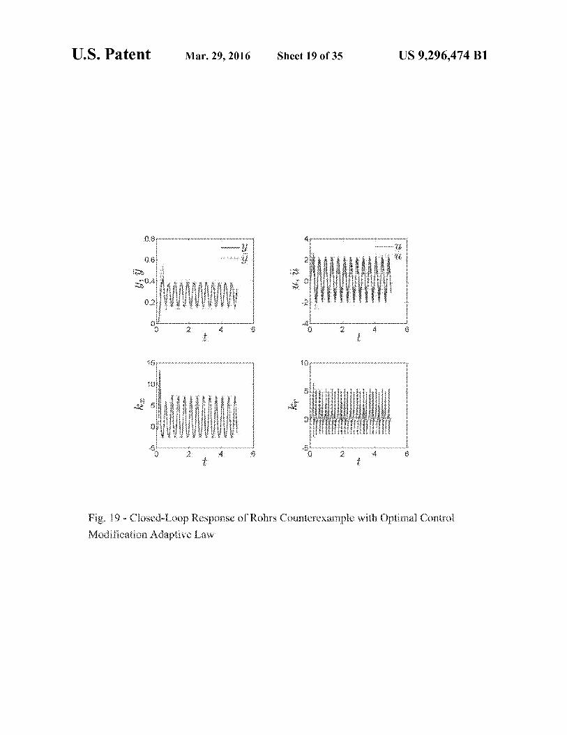
Fig. 19 - Closed-Loop Respoiise of Robrs Counte•exaniple with Optimal Control

Modiflication Adaptive Law


2

1.5

x 1

0,5

0 0 5 10 15 20 25 30 35 40

t

0

-0.2

-0.4

-0.6

-0,8 0 5 10 15 20 25 30 35 40

t

Fig. 20 -INon-Minimum Phase Adaptive Control System with Optimal Control

U.S. Patent Mar. 29 , 2016 Sheet 21 of 35

US 9,296,474 B1

Modification Adaptive Law 115

Reference Model

r~

110 105 ~~Yzfi

Adaptxve .(~ roller

Uncertain Plant

120, 150, 155, 1604 170

Optimal (control Modification

Covariance Adjustment

.Adaptive Control System 100

Fig. 2:1- Adaptive Control System with Optimal Modification Adaptive Law and Covariance Adaptive Gain Adjustment Method


115

Reference Model

------------------------------------------------

110 /-,1, 105 TI

Adap~IiVe Uncertain Plant

120,1500155,160,170

Optimal Contr©l Modification

Adaptive Gain Normalization

205

Adaptive Control System 100

Fig. 22 - Adaptive Control System with Optimal Modification Adaptive Law and Adaptive Gain Normalization Method


2302

.x-•fir 2301

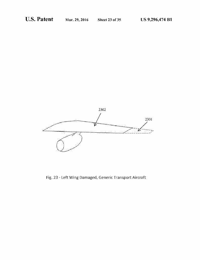
Fig, 23 _ Left Wing Damaged, Generic Transport Aircraft


US 9,296,474 B1

20 20 ----- --------- 1 -------- ----- PM

10 10

. t

cz -10

° -10

Baseline Controller -20 -20

0 10 20 30 40 0 t, sec

10 20 30 40 i, SGC

20 20

R Pm P P, 10 10

cn

-10 OCIM Covariance Update -10 OCM Normalization F =3000, v=0.2, =0,0126

-20 -2t3 0 10 20 30 40 0 10 20 30 40

t, sec

Fig. 24 - Boll Rate Responses due to Left Wing Damage

4

2

o

-2

h

0 10 20 30 40

t, sec


Sheet 25 of 35 US 9,296,474 B1

- 4,

n~ 4 grr3 2

0 0

i OCP~

~

t[~

Co

vadance Update ~Cry

hb~€~3

€~~

c ~,ap

lizatii -~

~r T' =3 ?00, v=0.2, 11-0.0 26 '~ 'I F=3000, v=0.2 1 R=1 00 -4

0 1 0 20 0 O y 0 1 0 20 30 t, sec t, sec

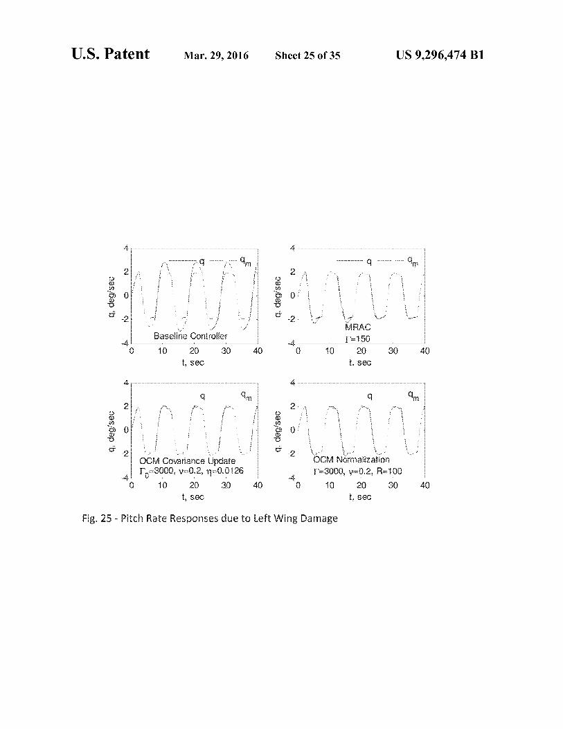
Fig. 25 -Pitch Rate Responses due to Left Wing Damage

40

r -------- --,, r F31

-3,4

0,2

0

-0,2


Sheet 26 of 35 US 9,296,474 BI

10 20 30 40 0 10 20 30 40 t, sec t ! see

0.4

0.2

'6 0

-!-, -A

- - - - - - - - - - - - - - - r ------ ----- r rn

OCM Covariance Update Fo=3000. v=0.2, ii=0.0126

---------------- - --------------------------------- -----------------

O.4

--------------- r -------- ----

0.2 - CIi tfr

-0,2 OCVII Normalization F=3000, v=0.2, R=1010

-0 4.._________________ -------------- ------------------ 0 10 20 30 40 0 10 20 30 40

1, see t, Sec

Fig. 26 - Yaw Rate Responses due to Left Wing Damage

F=3000, v=0.2, R=-100 ------

O ------- ---- m

0- 10 20 30 40 C. 10 20 30 40

t, See t, see

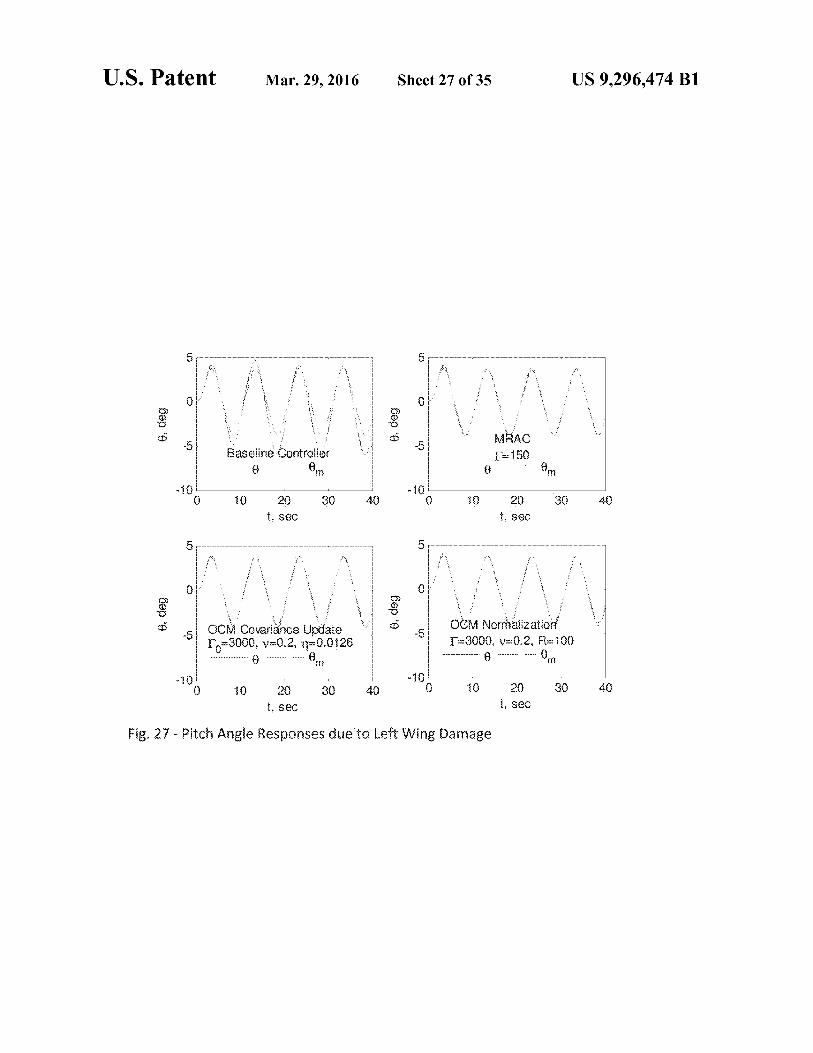
Fig, 27 - Pitch single Responses due to Left Wing Damage

10 20 30 40 t. sec

10 20 30 40 sec

40~

0

r zs

5

0

5

0 a~

5

.I 0 t

5

0

-5

5

G

-10

U.S. Patent Mar. 29 , 2016 Sheet 27 of 35 US 9 ,296,474 B1

20

10

0

10

-20

-QrI 10 20 30 40 0

t 5 Sec 10 20 30 40

k, SeC

0

-20

-40 L


20

10

0

10

-20

-I~n

OCM Covariance Update FO=3000, v=02, -q=0.0126

20

10

0

-20

~n

OCVI Normalization r=3000, v=0.2, R=100

10 20 30 40 0 10 20 30 40 t, Sec t, Sec

Fig. 28 - Bank Angle Responses dLJe to Left Wing Damage


30

20

0) 10,

C~ 0

10

20

30 :-

Baseline Controller 20:~

U) 10 :: CD

-

0 10 20 30 40 -e_u

0 t, see

10 20 30 40

40

20

0)

OCM Covariance Update I",,=3000, v=0.2, 3l=0.0126

30 -

20:1

10 ::

0 :

-10'4

-20 L 0 10 20 30 40 0 10 20 30 40

t, sec t, sec

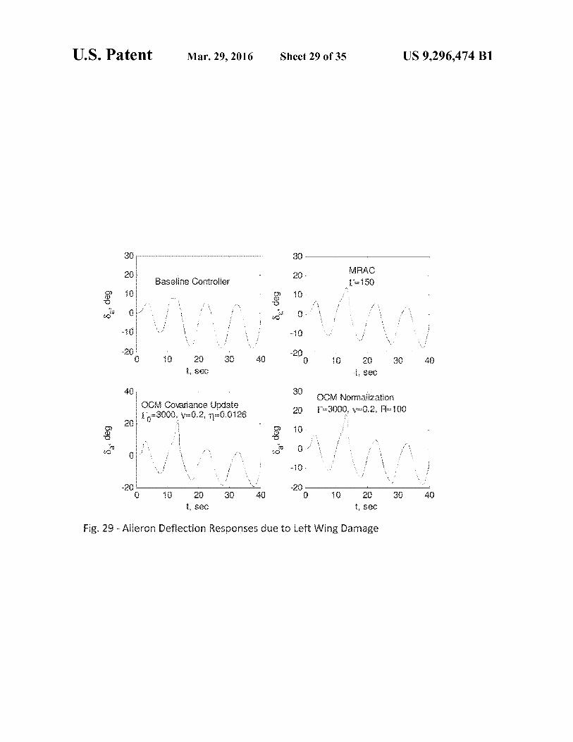
Fig. 29 - Aileron Deflection Responses due to Left Wing Damage

4 4

2 g:

0

-2

-4 - 0 1C 20 30 40

t, sac


Sheet 30 of 35

US 9,296,474 B1

4

4

Cl7

2

CJ , L / J

t Cell C~7uarianc6 ~ ate 2 ti

P OCM Norrnaiizalion

-4 l a=300 3 ; v40.2, -0.0126

4 F=3000, v=0.2, R=100

0 10 20 30 40 0 10 20 30 40 t, sac t, sec

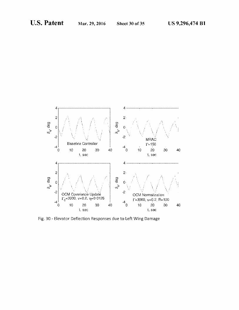
Fig. 30 - Elevator Deflection Responses due to Left W ing Damage

5

0 CD Q>

-5

-10 L (3

4

2

70 70

-2

--4

-rI 10 20 30 40 0

t, sec

Iii RAC; 1'--150

10 20 30 40 t, seo


Sheet 31 of 35 US 9 ,296,474 B1

4

4

2 OCM Cowriance update

2 C_3CM Normaiization

zn (~ 17,=3000, v=0.2, il=0,0126

0 1'=30€30. v=0.2, R=100

c -2 e -2

-4 -4

-6 -6 0 10 20 30 40 0 10 20 30 40

t, sac 1, sec

Fig. 31 - Rudder Deflection Responses due to Left Wing Damage


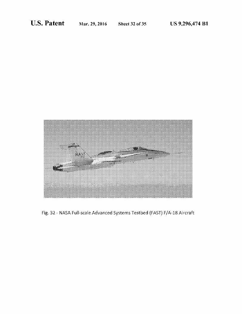
Fig. 32 -NASA Full-scale Advanced Systems Testbed (FAST) F/A-18 Aircraft

U.S. Patent Mar. 29 2016 Sheet 33 of 35 US 9,296,474 BI

25)`1 235

245 225

230

IAxo : :1111

250

1!'Iversion AdaW~ Rpin' 'ContNer 2 1 0

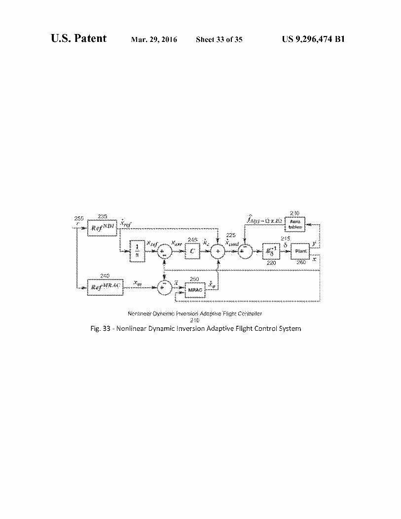
Fig. 33 - Nonlinear Dynamic Inversion Adaptive Flight Control System


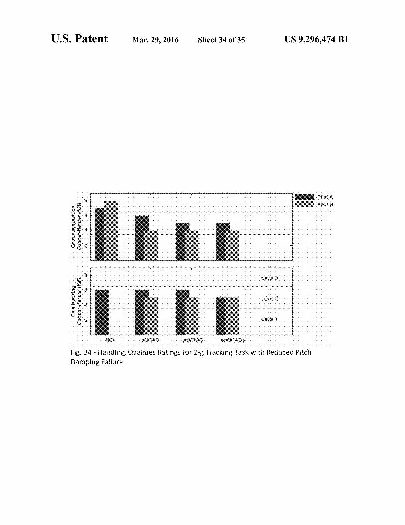
Fi& 34 - Handling Qualities Ratings for 2-g Tracking Task with Reduced Pitch Damping Failure


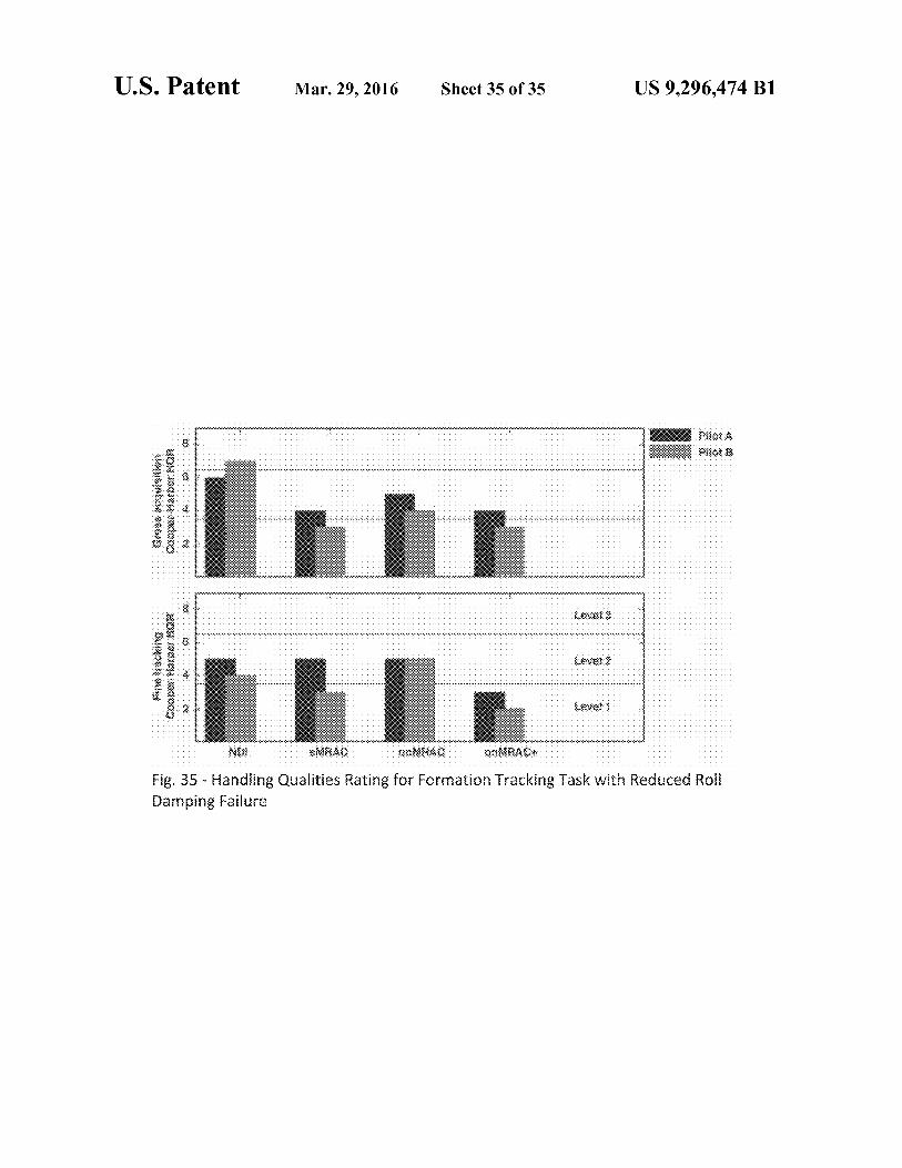
Fig. 35 - Handling Qualities Rating for Formation Tracking Task with Reduced Roll Damping Failure

US 9,296,474 B1

CONTROL SYSTEMS WITH NORMALIZED AND COVARIANCE ADAPTATION BY

OPTIMAL CONTROL MODIFICATION

CROSS-REFERENCE TO RELATED 5 APPLICATIONS

The present invention is based upon and claims priority from prior U.S. Provisional Patent Application No. 61/679, 945, filed onAug. 6, 2012 and U.S. Provisional PatentAppli- 10 cation No. 61/798,236, filed on Mar. 15, 2013, the entire disclosure of which are herein incorporated by reference in their entirety.

ORIGIN OF INVENTION 15

The invention described herein was made by employees of the United States Government and may be manufactured and used by or for the Government of the United States of America for governmental purposes without the payment of 20

any royalties thereon or therefore.

BACKGROUND

The present invention relates to control systems for 25

dynamic systems and more specifically to adaptive control systems for an aircraft or, more generally, a flight vehicle.

Feedback control systems are used to control and improve stability of many physical systems such as flight vehicles. Conventional feedback controls are typically designed using 30

a set of constant-value control gains. As a physical system operates over a wide range of operating conditions, the values of the control gains are scheduled as a function of system parameters. This standard approach is known as gain-sched-uled feedback control. A conventional feedback control SyS- 35

tem generally requires a full knowledge of a physical system for which the control system is designed. Under off-nominal operating conditions when a system experiences failures, damage, degradation, or otherwise adverse events, a conven-tional feedback control system may no longer be effective in 40

maintaining performance and stability of the system. Adaptive control has been developed to provide a mecha-

nism for changing control gains on line by adaptation to the system uncertainty. Thus, one advantage of adaptive control is its ability to control a physical system that undergoes Sig- 45

nificant, but unknown changes in the system behaviors. The ability to adjust control gains online makes adaptive control an attractive technology that has been receiving a lot of inter-ests in the industry. Yet, despite the potential benefits, adap-tive control has not been accepted as a mature technology 50

which can be readily certified for deployment in mission-critical, safety-critical or human-rated systems such as air-craft flight control systems. A number of challenges presently exist such as the following:

One of problem that has not been well addressed is the 55

adverse effect of persistent excitation. In a nutshell, persistent excitation is a condition that relates to the richness of input signals to a control system. During adaptation, some degree of persistent excitation must exist in an input signal to enable a human operator or an adaptive control system to learn and 60

adapt to the changing environment. However, an excessive degree of persistent excitation can adversely affect stability of the system. The possibility of excessive persistent excitation can exist in off-nominal systems with human operators in the loop who sometimes can unknowingly create persistently 65

exciting large input signal in order to rapidly adapt to the changing environment.

2 Another important problem that exists in adaptive control

is the complex nature of the input-output signals, which are inherently nonlinear. The complex, nonlinear input-output mapping of many adaptive control methods can lead to an unpredictable behavior of a control system. To this extent, an operator cannot learn from a past response to predict what a future response will be. In contrast, a linear input-output mapping is highly desirable since the knowledge from a past response can be used to predict a future response. Conse-quently, adaptive control systems tend to be unpredictable and inconsistent in their behaviors. The predictability of a control system is a crucial element in the operation of a control system that involves a human operator such as an aircraft pilot or an automobile driver. Unpredictability can result in over-actuated or under-actuated control signals which both can lead to undesirable outcomes and potentially catastrophic consequences.

The sensitivity of adaptive control systems to large inputs and persistent learning is another important consideration. Because of the nonlinear behaviors, large inputs can lead to deleterious effects on adaptive control systems. A physical system may be stable when small amplitude inputs are used in adaptive control, but the same system can become unstable when the input amplitude increases. The amplitude of an input can be difficult to control because it can be generated by a human operator like a pilot. Persistent learning is referred to the process of constant adaptation to small error signals. In some situations, when an adaptive control system has achieved sufficient performance, the adaptation process needs to be scaled down. Maintaining a constant state of fast adaptation even after the errors have diminished can result in persistent learning. At best, persistent learning would do nothing to further improve the performance. At worst, persis-tent learning reduces robustness of an adaptive control system by constantly adapting to small error signals.

The most fundamental issue is the lack of metrics to assess stability of an adaptive control system. Currently, there are no well-established metrics or methods for analyzing thereof that can satisfy conventional certification requirements for adaptive control. Unlike conventional classical linear control which is endowed with many important and useful tools for analyzing performance and stability certification require-ments of a closed-loop system, adaptive control suffers a disadvantage of the lack thereof. Consequently, there is cur-rently no fielded adaptive control system certified for use in any production system.

A distinct feature of a typical adaptive control design is the ad-hoc, trial-and-error nature of the design process which involves selecting suitable design parameters such as the adaptive gain, or adaptation rate, without analytical methods for guiding the design. A trial-and-error design process may enable an adaptive control system to work well under a design conditions, but by the same token may fail to work well under other conditions. As a result, this ad-hoc process tends to make the design of adaptive control to be particularly difficult to implement by general practitioners of control systems.

There exist several robust modification adaptive control methods. The two most popular conventional methods are the a-modification and the e-modification. Both or these meth-ods were established in the 1980's. The a-modification adap-tive control provides a constant damping mechanism to limit the adaptation process from becoming unstable, and the e-modification provides a damping mechanism that is pro-portional to the norm of the tracking error signal to accom-plish the same. The projection method is another popular method that is used to bound adaptive parameters to prevent

US 9,296,474 B1 3

issues with persistent learning. As with most adaptive control methods, the aforementioned challenges exist in one form or another.

BRIEF SUMMARY

A novel method for improving performance and stability of control systems has been developed. This method represents a significant advancement in the state-of-the art in adaptive control technology. The present invention discloses a new type of adaptive control law, called optimal control modifi-cation, which blends two control technologies together: opti-mal control and adaptive control. Unlike the prior art, the present invention provides: 1) the introduction of a damping mechanism that is proportional to a property known as per-sistent excitation to improve robustness of adaptation in the presence of persistently exciting signals, 2) the existence of linear asymptotic properties that make the method well suited for design and analysis for performance and stability guaran-tee, and 3) the use of a time-varying adaptive gain by two methods: normalization and covariance adjustment to further improve stability of the control systems in the presence of time delay and unmodeled dynamics.

The method has gone through a series of validation process ranging from many desktop aircraft flight control simulations to a pilot evaluation in high-fidelity motion-based Advanced Concept Flight Simulator at NASA Ames that culminated in a recent flight test program on a NASA F/A-18A research test aircraft. The successful pilot-in-the-loop flight test of the optimal control method on the NASA F/A-18A aircraft rep-resents the further point in technology validation at NASA. No other adaptive control method in the field is presently known to have gone through a validation process this far that involves flight testing on a human-rated high-performance aircraft.

BRIEF DESCRIPTION OF THE SEVERAL VIEWS OF THE DRAWINGS

The accompanying figures where like reference numerals refer to identical or functionally similar elements throughout the separate views, and which together with the detailed description below are incorporated in and form part of the specification, serve to further illustrate various embodiments and to explain various principles and advantages all in accor-dance with the present invention, in which:

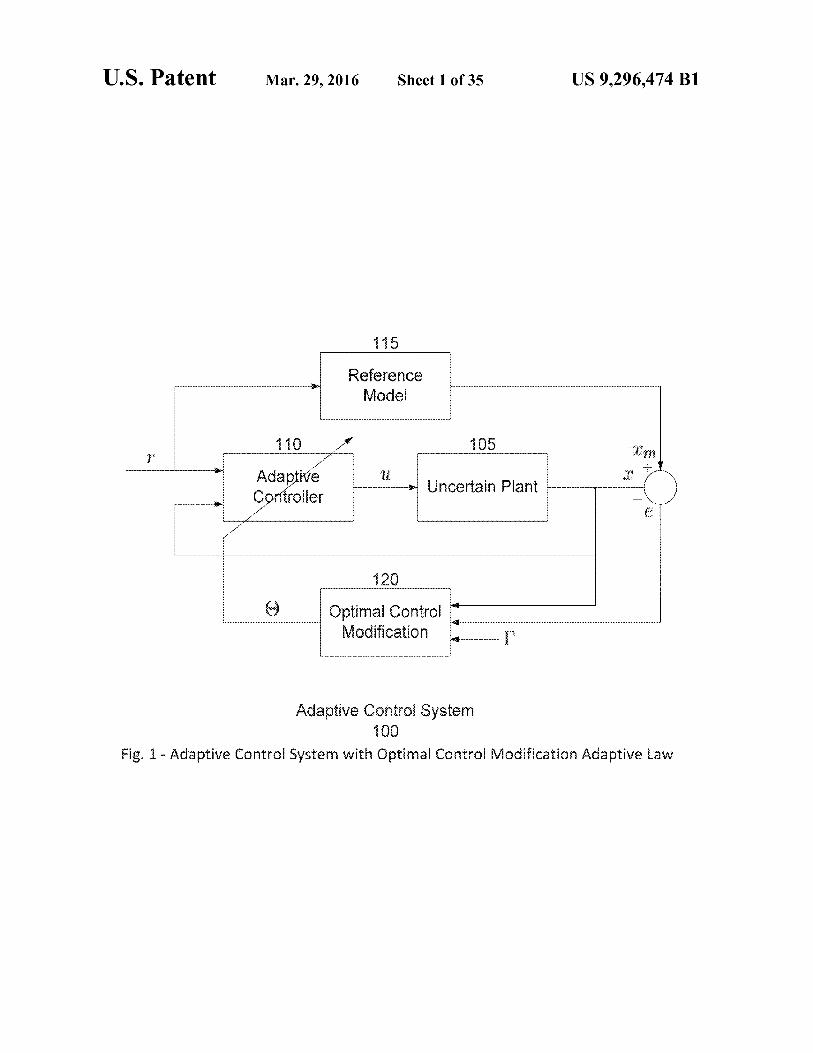
FIG. 1 illustrates a block diagram of an adaptive control system with the optimal control modification adaptive law as taught by the present invention;

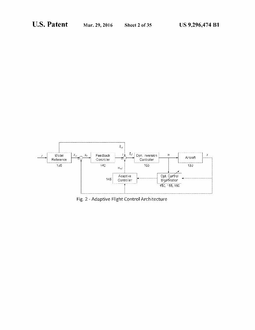
FIG. 2 illustrates a block diagram of a dynamic inversion adaptive flight control architecture;

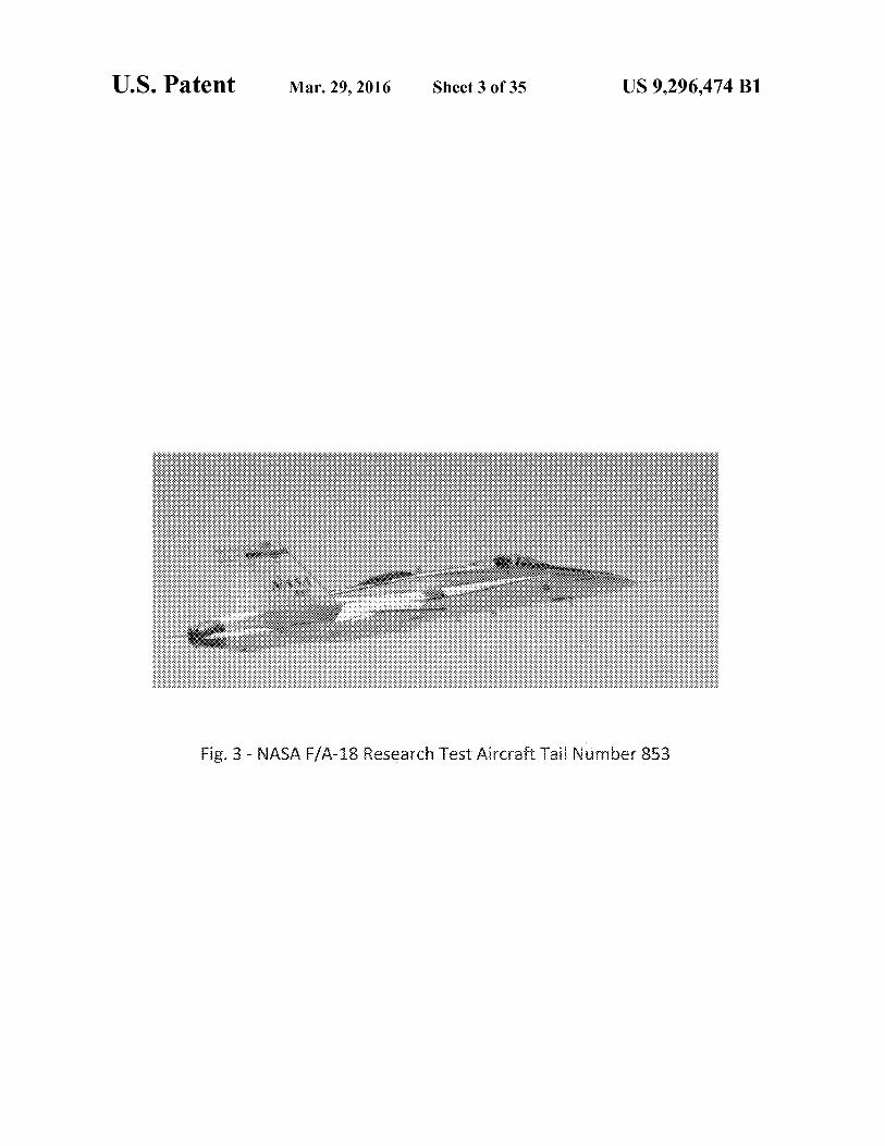
FIG. 3 is a photograph of the NASA F/A-18 research test aircraft, tail number 853; which is the subject aircraft for the application of the present invention;

FIG. 4 is the plot of the time history of the longitudinal states due to an A-matrix failure (C ma shift at 13 sec) in the NASA F/A-18 model with and without the optimal control modification adaptive law;

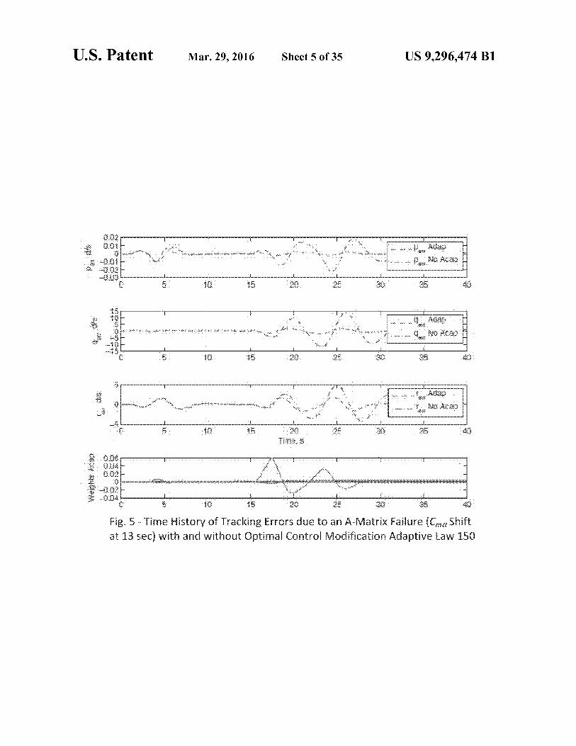
FIG. 5 is the plot of the time history of the tracking errors due to an A-matrix failure (C ma shift at 13 sec) in the NASA F/A-18 model with and without the optimal control modifi-cation adaptive law;

FIG. 6 is the plot of the time history of the control surfaces due to an A-matrix failure (C ma shift at 13 sec) in the NASA F/A-18 model with and without the optimal control modifi-cation adaptive law;

4 FIG. 7 is the plot of the time history of the longitudinal

states due to a B-matrix failure (stabilator jammed at 2.5° at 113 sec) in the NASA F/A-18 model with and without the optimal control modification adaptive law;

5 FIG. 8 is the plot of the time history of the lateral-directional states due to a B-matrix failure (stabilator jammed at 2.5° at 13 sec) in the NASA F/A-18 model with and without the optimal control modification adaptive law;

FIG. 9 is the plot of the time history of the tracking errors 10 due to a B-matrix failure (stabilator jammed at 2.5° at 13 sec)

in the NASA F/A-18 model with and without the optimal control modification adaptive law;

FIG. 10 is the plot of the time history of the pitch rate error 15 and weights due to an A-matrix failure (C ma shift at 2 sec) in

the NASA F/A-18 model with the optimal control modifica-tion adaptive law (F-0.5 and E=50 with fixed v=1);

FIG. 11 is the plot of the time history of the pitch rate error and weights due to an A-matrix failure (C ma shift at 2 sec) in

20 the NASA F/A-18 model with the optimal control modifica-tion adaptive law (Fixed F -5 with v-0.25 and v=1);

FIG. 12 is a photograph of the Advanced Concept Flight Simulator at NASA Ames Research Center in which a pilot study was conducted to evaluate the optimal control modifi-

25 cation adaptive law among six other adaptive controllers; FIG. 13 is the pilot Cooper-Harper Ratings of the seven

adaptive flight controllers evaluated by 8 NASA test pilots in the Advanced Concept Flight Simulator;

FIG. 14 is the plot of the response of a first-order SISO 30 plant with the optimal control modification adaptive law with

a time delay td-0.0020 sec showing the agreement between the analytical values and the numerical values of the steady state error and the equilibrium value of the adaptive param-eter;

35 FIG. 15 is the plot of the response of a first-order SISO plant with the optimal control modification adaptive law with a time delay td-0.2795 sec showing the agreement between the analytical value and the numerical value of the time-delay margin;

40 FIG. 16 is the plot of the response of the same first-order SISO plant with the optimal control modification adaptive law showing the existence of a scaled input-output property of the optimal control modification adaptive law and the lack thereof of the prior art a-modification and e-modification;

45 FIG. 17 is the plot of the response of the first-order SISO plant with unmodeled dynamics in the Rohrs counterexample illustrating the instability phenomenon of standard model-reference adaptive control;

FIG. 18 is the plot of the phase margin and the cross-over 50 frequency of the Rohrs counterexample as analytically com-

puted from the linear asymptotic property of the optimal control modification adaptive law as taught by the present invention;

FIG. 19 is the plot of the response of the first-order SISO 55 plant with unmodeled dynamics in the Rohrs counterexample

of Rohrs Counterexample showing stability and the agree-ment between the analytically predicted output and the numerically computed output with the optimal control modi-fication adaptive law;

60 FIG. 20 is the plot of the response of a non-minimum phase first-order SISO plant illustrating an analytical method for computing the modification parameter v to ensure stable adaptation for a non-minimum phase plant;

FIG. 21 illustrates an adaptive control system with the 65 optimal control modification adaptive law that further

includes the covariance adaptive gain adjustment method as taught by the present invention;

US 9,296,474 B1 5

6 FIG. 22 illustrates an adaptive control system with the an adaptive control system to learn, the present invention will

optimal control modification adaptive law that further provide an effective damping mechanism to counteract any includes the adaptive gain normalization method as taught by adverse effects of persistent excitation that can lead to insta- the present invention; bility.

FIG. 23 illustrates a partial left wing tip damage, which is 5 An important key enabling feature of the present invention the subject aircraft for the application of the present inven-

is the linear asymptotic property. For a linear plant with tion; uncertainty, the optimal control modification approaches

FIG. 24 is the plot of the roll rate responses due to the left asymptotically to a linear control system under fast adapta-

wing damage for four different flight controllers; tion. The condition of fast adaptation means that the rate at

FIG. 25 is the plot of the pitch rate responses due to the left io which the adaptive parameters rule estimated by the optimal wing damage for four different flight controllers; control modification is sufficiently large relative to the rate of

FIG. 26 is the plot of the yaw rate responses due to the left

the system response. With fast adaptation, the behavior of the wing damage for four different flight controllers; optimal control modification is asymptotically linear. This

FIG. 27 is the plot of the pitch angle responses due to the feature is the most unique attribute as compared to any other

left wing damage for four different flight controllers;

15 existing conventional adaptive control methods, with the FIG. 28 is the plot of the bank angle responses due to the exception of the LI adaptive control. This feature affords a

left wing damage for four different flight controllers; number of advantages. First and foremost, the optimal control FIG. 29 is the plot of the aileron deflection responses due to modification substantially reduces the complex nonlinear

the left wing damage for four different flight controllers; input-output mapping of conventional adaptive control meth-

FIG. 30 is the plot of the elevator deflection responses due 20 ods. The asymptotic linear property therefore makes the to the left wing damage for four different flight controllers; present invention much more predictable and consistent in its

FIG. 31 is the plot of the rudder deflection responses due to performance. the left wing damage for four different flight controllers;

Another key feature of the optimal control modification is FIG. 32 is a photograph of the NASA Full-scale Advanced

the use of normalization or covariance adjustment of time-

Systems Testbed (FAST) F/A-18 research test aircraft, tail 25 varying adaptive gain to reduce adverse effects of large ampli- number 853; tude inputs and persistent learning. The normalization effec-

FIG. 33 is the block diagram of the nonlinear dynamic tively modifies the adaptive gain by dividing the adaptive gain

inversion adaptive flight control system implemented on by the squares of the input amplitudes, so that the optimal

NASA FAST aircraft employing the optimal control modifi- control modification is much less sensitive to large amplitude cation adaptive law with the adaptive gain normalization;

30 inputs. As a result, the optimal control modification can

FIG. 34 is the plot of the handling qualities ratings for a 2-g achieve a significant increase in stability margins. Another tracking task with a reduced pitch damping failure; and

method for improving stability margins by eliminating or FIG. 35 is the plot of the handling qualities rating for a reducing persistent learning is the covariance adjustment

formation tracking task with a reduced roll damping failure. method. During adaptation, the covariance adjustment 35 method continuously adjusts the adaptation rate or adaptive

DETAILED DESCRIPTION

gain from an initial large value toward a final lower value. Thus, once the adaptation has achieved its objective of restor-

The present invention addresses the current problems in

ing performance, a large adaptive gain is no longer needed adaptive control technology with a novel adaptive control

and therefore should be reduced. As a result, a significant

method, called optimal control modification which blends 40 increase in robustness is attained. two control technologies together: optimal control and adap- In regards to the lack of metrics for stability and methods tive control. The key features that differentiate this invention

for analyzing thereof, the linear asymptotic property of the

from the prior art are: 1) the introduction of a damping mecha- optimal control modification affords an important advantage. nism that is proportional to property known as persistent

Stability of conventional model-reference adaptive control

excitation to improve robustness of adaptation in the presence 45 generally decreases with increasing the adaptive gain. In the of persistently exciting signals, 2) the linear asymptotic linear

limit, a stability margin of the standard model-reference

property that makes the method more amenable to perfor- adaptive control tends to zero as the adaptive gain becomes mance and stability analysis in a linear context, and 3) the use

infinitely large. With fast adaptation, the adaptive gain is

of a time-varying adaptive gain by two methods: normaliza- assumed to be infinitely large or much larger than the rate of tion and covariance adjustment to further improve stability of 50 the system response. Then, the optimal control modification the control systems in the presence of time delay and unmod- tends to a linear control system. The feedback control system eled dynamics. in the limit behaves as a linear control system, unlike most

The present invention addresses specifically to current conventional adaptive control methods. Because the feedback challenges with adaptive control in these areas: 1) persistent control system is asymptotically linear, there exist many well- excitation, 2) complex nonlinear input-output mapping, 3) 55 accepted metrics for analyzing stability of such systems. large inputs and persistent learning, and 4) the lack of stability

These stability metrics are used in many well-established

analysis tools for certification. The invention has been subject control system specifications such as MIL-SPEC. Moreover, to many simulations and flight testing. The results substanti- there are many widely available methods for analyzing sta- ate the effectiveness of the invention and demonstrate the

bility of linear control systems. Thus, the present invention

technical feasibility for use in modem aircraft flight control 60 can potentially address the lack of a certification process for systems. adaptive control by leveraging the linear asymptotic property

The present invention successfully addresses the existing to enable adaptive control based on the present invention to be problems with the following unique features: analyzed using well-established metrics for stability and

The optimal control modification provides robustness to methods for analyzing thereof. persistently exciting input signals by adding a damping 65 This innovation is expected to have a wide range of com- mechanism proportional to the persistent excitation quantity. mercial potential applications in aerospace industry, transport Thus, as apersistently exciting input signal is applied to allow vehicle industry, etc. In particular, flight control is one area of

US 9,296,474 B1 7

major interest and high potential applications. Aviation indus-try which may be interested in this technology includes Boe-ing, Honeywell, and others. NASA aviation safety research as well as space launch vehicle system development could be potential users of this technology.

Optimal Control Modification Adaptive Control Learning is an optimization process that attempts to recon-

struct a model of a system which operates in an uncertain environment. The optimization process is designed to mini-mize the error between the model of the system and the actual observed behaviors of the system. The optimality of the pro-cess results in a mathematical law that describes the adapta-tion or learning process. Therefore, the notion of optimization is a fundamental principle of system identification or param-eter estimation techniques which can be viewed as an adap-tation process.

The notion of optimization is generally not considered in the standard model-reference adaptive control. The param-eter estimation process based on the standard model-refer-ence adaptive control approach is usually driven by the error between the reference model outputs and the actual system outputs, known as tracking error. The learning or adaptive law is effectively a nonlinear parameter estimation process. Asymptotic tracking, which is referred to the tracking error tending to zero in the limit, is an ideal behavior of the standard model-reference adaptive control which can be achieved if the structure of the uncertainty is known. However, with uncertainty with unknown structures or unmodeled dynam-ics, the standard model-reference adaptive control can become unstable.

Parameter drift is a numerical phenomenon in adaptive control that results in a blow-up of adaptive parameters. This blow-up is caused by the ideal behavior of asymptotic track-ing of the standard model-reference adaptive control which results in infinite adaptive parameters in an attempt of seeking a zero tracking error in the limit. This can be mathematically illustrated by a simple control system expression:

z=ax+bu+w (1)

u=-k (t)x (2)

where kx(t) is an adaptive feedback gain which can be computed by the standard model-reference adaptive control.

For a sufficient large disturbance, the standard model-ref-erence adaptive control attempts to generate a high-gain con-trol in order to reduce the effect of the disturbance. In the limit, the steady-state solution of x is obtained as

w (3) — = r~~ a - kx (t)

In order to seek a zero solution in the limit, k x(t) must tend to a very large value in the limit. Thus, the standard model-reference adaptive control can cause k x(t) to become unbounded. In practice, a high-gain control with a large value of kx(t) can be problematic since real systems can include other closed-loop behaviors that can lead to instability when k(t) becomes large. Thus, parameter drift can lead to instabil-ity in practical applications.

As the complexity of a control systems increases, robust-ness of adaptive control becomes increasingly difficult to ascertain. By definition, robustness is the ability for a control system to remain stable in the presence of unstructured uncer-tainty and or unmodeled dynamics. In practical applications, the knowledge of a real system can never be established exactly. Thus, a mathematical model of a physical system

8 often cannot fully capture all the real, but unknown effects due to unstructured uncertainty and or unmodeled dynamics. All these effects can produce unstable closed-loop dynamics using the standard model-reference adaptive control.

5 The present invention takes advantage of the notion of optimization or optimal control to improve robustness of adaptive control by means of the development novel adaptive control method called optimal control modification. The opti-mization framework is posed as a minimization of the L 2

io norm of the tracking error bounded away from the origin by a finite distance. This distance is a measure of robustness. Thus, the optimization is designed explicitly to trade away the ideal property of asymptotic tracking of the standard model-refer-ence adaptive control for improved robustness by minimizing

15 the following cost function:

r

J = fim 1 f (e - 0)T Q(e - 0)dt ( )

r~~ 2 0

20

where e(t) is the tracking error and A(t) is an unknown lower bound of the tracking error, which represents a distance from the origin.

25 By avoiding asymptotic tracking, the present invention can achieve improved robustness while maintaining sufficient performance with bounded tracking error. In fact, almost all conventional robust adaptive control methods achieve bounded tracking as opposed to asymptotic tracking in

30 exchange for improved robustness. Unlike many conven-tional robust adaptive control methods, the present invention accounts for bounded tracking explicitly in an optimization framework.

To further elucidate the novelty of the present invention, 35 refer to FIG. 1 which illustrates an adaptive control system

100 of the present invention. The adaptive control system 100 further comprises a nonlinear plant 105, an adaptive control-ler 110, a reference model 115, and an optimal control modi-fication adaptive law 120 as taught by the present invention.

40 The nonlinear plant 105 with a matched uncertainty and an

unmatched disturbance is described mathematically as

z=Ax+B[u+O *T(D(x)]+w (5)

where x(t) is a state vector, u(t) is a control vector, A and B 45 are known matrices such that the pair (A,B) is controllable,

O* is an unknown constant ideal weight matrix that repre-sents aparametric uncertainty, (D(x) is a vector of knownbasis functions that are continuous and at least in C i , and w(t) is a bounded disturbance with an upper bound w,

50 The feedback adaptive controller 110 represented by u(t), is designed to achieve a command-following objective as

u=-K,x+K,r-u, (6)

where r(t) is a bounded command vector, K x is a stable 55 feedback gain matrix such that A—BK x is Hurwitz, K,, is a

command feedforward gain matrix, and uad(t) is an adaptive control signal of the present invention which estimates the parametric uncertainty in the plant as

60 uQ -O T(D(x)

(7)

where O(t) is an estimate of the parametric uncertainty E)*. The adaptive controller 110 is designed to follow the ref-

erence model 115 which is defined as

65 zm =Amxm +Bmr (8)

where A_=A—BKx and Bm=BK,..

US 9,296,474 B1 9 10

Let 0=0-0* be an estimation error of the parametric The bound on A(t) as tf-- can be estimated by uncertainty and e--xm -x be the tracking error, then the tracking error equation becomes

T 17

e=Ame+B6 7(D (x) -w (9) 5 11A11 < Ai, (Q)

d("'(x)) +IIP11(IIB11110*1111 (D (x)11 +wo)1 ( )

The optimization can be formulated as a dynamically con-strained optimization problem using the Pontryagin's Maxi-mum Principle. Towards that end, defining a Hamiltonian

H(e,6)=112(e—A) 7Q(e—A)+p 7(t)[A m e+B67(D(x)—w] (10)

where p(t) is an adjoint variable. Then the adjoint equation can be obtained from the neces-

sary condition as

P=-VH T-- Q* (e— A) — Am TP (11)

with the transversality condition p(t,--)O since e(0) is known.

The optimal control modification adaptive law 120 can then be formulated by a gradient method as

6=ry HOT =-r(D(x)p 7B (12)

where F-F'>0 is a constant positive -definite adaptive gain matrix.

A sweep method can be used to obtain an approximate solution of the adjoint variable. Upon analysis, it can be shown that the adjoint variable p(t) is obtained as

p=Pe—vAm 7PB0 7(D(x) (13)

where v>0 is the modification parameter which is a design free parameter such that v=1 corresponds to the approximate optimal solution and v;-I corresponds to a sub-optimal solu-tion, and P=P T>0 is a positive-definite matrix which solves the following Lyapunov equation:

PAm +Am 7P+Q=0 (14)

where Q-QT>0 is a positive-definite weighting matrix. This leads to the following optimal control modification

adaptive law 120 which is the basis of the present invention:

0=I'(D(x)[e7P—v(D 7(x)OB TPAm ']B (15)

The inputs of the optimal control modification adaptive law 120 are the tracking error e(t) and the basis function (D (x). The design parameters of the optimal control modification adap-tive law 120 are the adaptive gain matrix L, the weighting matrix Q which influences the Lyapunov matrix P, and the modification parameter v.

In the expression of the optimal control modification adap-tive law 120, the first term inside the bracket is the standard adaptive law. The second term is the result of the optimiza-tion . This term is referred to as the optimal control modifica-tion term. Contained therein is a product term (D(x)( T(x) whichrepresents the effect of a persistent excitation condition

Illf o 10+7(D(x)(D 7(x)dtaal (16)

Thus, the optimal control modification term effectively provides a damping mechanism that is proportional to the persistent excitation to reduce the adverse effect thereof on adaptive control.

The role of the modification parameter v is important. If performance is more desired in a control design than robust-ness, then v could be selected to be a small value. In the limit when v-0, the standard model-reference adaptive control is recovered and asymptotic tracking is achieved but at the expense of robustness . On the other hand , if robustness is a priority in a design, then a larger value of v can be chosen.

which is dependent upon the modification parameter v, the norm of the parametric uncertainty I JO *1 1, and the upper bound

10 of the disturbance w,

The optimal control formulation of the optimal control modification codification adaptive law 120 thus shows that ~JA(t)JJ will always remain finite as long as the uncertainty and

15 or the disturbance exists. Therefore , bounded tracking as opposed to asymptotic tracking is better achieved with the optimal control modification adaptive law 120 to improve robustness. In contrast , the standard model-reference adap-tive control can achieve the ideal property of asymptotic

20 tracking if the disturbance w(t)O, but usually at the expense of robustness to unmodeled dynamics, time delay, and exog-enous disturbances. In the presence of the disturbance w(t), the standard model-reference adaptive control can result in a parameter drift when the adaptive parameter O(t) can grow

25 unbounded. Thus, in many real systems, asymptotic tracking is a very demanding requirement , if not almost impossible, that usually cannot be met without any restrictions. The opti-mal control formulation of the optimal control modification adaptive law 120 therefore demonstrates that bounded track-

30 ing is a more realistic control objective if robustness is to be satisfied concurrently. Since IJAII is proportional to the modi-fication parameter v, the optimal control modification adap-tive law 120 canbe designed judiciously to trade performance with robustness. Increasing the value of the modification

35 parametery will reduce tracking performance but by the same token increase robustness. This trade -off generally exists in most feedback control systems but the standard model-refer-ence adaptive control.

40 Using the standard Lyapunov stability theory, it can be shown that the optimal control modification adaptive law 120 is stable and results in an uniformly ultimately bounded track-ing with the following ultimate bound:

45

;L._ (p)62 +;mctt(r 1)K2 (1 g) Ilell ~ P =

50 where

vcc2 (19)

2 4 6=C2+ C2+

C

C, C2 (20) K = C4+VC4

VC

60 for any modification parameter 0<v<vm_, where

Ct =';L i,(Q), C2 = A,»~(~wo

65

c,=k_JBTA_-TQ` _-'B)q)02'

0 Am

- f l

-

/

55 L - K Kv J

B- ~ 0

(38)

(39)

US 9,296,474 B1 11 12

short-period mode and the Dutch roll mode. The reference

JIB TPAm1BIIDo model 135 is a second-order model that specifies desired C4 = t ;,,(BTA-TQA-i B) ' handling qualities with good damping and natural frequency

characteristics as shown:

Oo maxJJE)*JJ, and II(D(x)11:5(Do• 5 (s2+2~PwPS+wP2)(Dm =g,6,, (28)

The stability proof uses the following Lyapunov candidate (

g s2 +2~ w +w e S (29)

function : g) -gg '°"

V(e,6)=e 7Pe+trace(6'F-6) (21) (s2+2~,w,s+w,2)Pm=9,6„ d (30)

Then, V(e,O) is evaluated as

V(e, 6)s-c. hell- c2)2 +c1c22-vc3(I#D ,4)2-C3c42 (22)

Let

Bb {(e,b):c. hell - c2)2+vc3(IOII -c4)2scic22+vc3c42} (23)

Then, V(e,O)>0 inside of B b, but V(e,O):50 outside B b . Therefore V(e,O) is a decreasing function outside of B b . This implies that trajectories (e(0),O(0)) will be uniformly ulti-mately bounded after some time t>T.

The maximum value of the modification parameter vm_ can be established to ensure the largest V(e,O):50. Then, for any 0<v<vmaz, J(D (x)JJ<(io is bounded.

The modification parameter v is dependent on the a priori knowledge of the bounds on the uncertainty as well as the disturbance to guarantee stability. Moreover , in the presence of a disturbance, i.e., c2;'01 then for the standard model-reference adaptive control which corresponds to v -0, K is unbounded. This implies an unbounded parameter variation for the standard model-reference adaptive control in the pres-ence of a disturbance . This observation is consistent with the parameter drift phenomenon.

Adaptive Flight Control with Optimal Control Modifica-tion Adaptive Law

Consider the following adaptive flight control architecture as shown in FIG. 2. The adaptive flight control architecture 125 comprises an aircraft plant 130, a reference model 135 that translates rate commands into desired acceleration com-mands, a nominal proportional -integral (PI) feedback con-troller 140 for rate stabilization and tracking, an adaptive controller 145 with the optimal control modification adaptive law 150 or its alternative embodiments 155 and 160, and a dynamic inversion controller 165 that computes actuator commands using desired acceleration commands.

Adaptive flight control can be used to provide consistent handling qualities and restore stability of aircraft under off-nominal flight conditions such as those due to failures or damage. Suppose the aircraft plant 130 is described by

10 where (D m, Om, and Rm are the reference bank, pitch, and

sideslip angles; cop , wg, and w,, are the natural frequencies for desired handling qualities in the roll, pitch, and yaw axes; ~P , fig, and s,, are the desired damping ratios; Slat,Sio ,and6,.ad are

15 the lateral stick input, longitudinal stick input, and rudder pedal input. and gP, gq, and g,, are the input gains.

Let p_-(D_, q_-O_, and r_--P_, then the reference model 135 can be represented as

zm =-KPxm -Kf o ixm dt+Gr (31)

20 where x_-[p_ qm r_ ] T Kp-diag(2~Pwp,2~^,2 ~ ), K -diag(wP2,Wg2,w,,2)-Q2 , G-diag(gp,gglgr), and r=[6,,, 6,,, 6—d]

In an alternative embodiment, the reference model 135 could be a first-order model in the roll axis as shown:

25

(s+0)P)Pm=g'6" (32)

Assuming the pair (A,,,B,) is controllable and the outer loop state vector z(t) is stabilizable , the nominal PI feedback controller 140, defined by u e, is given by

30

ue K,(x m -x)+Kfo`(xm -x)dt

(33)

and the adaptive controller 145, defined by uad(t), is given by

35 u,-6 1 T(D(x,z) (34)

Assuming B, is invertible, then the dynamic inversion con-troller 165 is computed as

u+Bj 1 (x_ A1lx-f112z +ue u,)

(35)

40 In a more general case when the control vector has more inputs than the number of states to be controlled , then an optimal control allocation strategy using a pseudo -inverse method is used to compute the dynamic inversion controller 165 as

45 u=Bt T(BtBt T) 1 (x.., Attx -Atzz+ue uQa) (36)

Let e-u.,(xm -x)dti xm -x] T be the tracking error, then the tracking error equation is given by

z=,4 1 1x+,412z+B. u+fi (xz)

24 e=Ame+B[o 1 T(D(xz) fl (xz)1

(37)

50 z=A21x+A22z+B2u+f2(xz)

(25) where

whereAli and B,, i=1,2, j=1,2 are nominal aircraft matrices which are assumed to be known, x=[p q r] T is an inner loop state vector of roll, pitch, and yaw rates; z=[A(D Aa AR AV Ah AO] T is an outer loop state vector of aircraft attitude angles, airspeed , and altitude ; a=[Aria Ab e A6,,] T is a control vector of aileron, elevator, and rudder deflections ; and f (x,z), i=1,2 is an uncertainty due to off-nominal events which can be approximated as

f(xz)_6*a T(D(xz)+E(x,z) (26)60 Let Q=2cI where c>0 is a weighting constant and I is an

identity matrix, then can be shown that where O*, is an unknown , constant ideal weight matrix,

and (D(x,z) is the input basis function vector chosen to be

(Dx T T T T T T x T K; 1 Kp + Kp 1 (K; + /) K, 1 (40)

( z)=[x px qx rx z u (z)] (27) 65 P = c

>0

K-1 K-1 (/ + K 1 ) The inner-loop rate feedback control is designed to p

improve aircraft rate response characteristics such as the

US 9,296,474 B1 13

-continued K: i (41)

PB=c Kpi (l+K; i )

B 7P4m iB=—cK z<0 (42)

Then, the optimal control modification adaptive law 150 for a nominal PI feedback controller is specified by

Oi —F[(D(x,z)e 7PB+"(x,z)(D 7(x,z)O JKs 2] (43)

which can also be expressed as

Oi —F[(D(x,z)e 7PB+"(x,z)(D 7(x,z)O 1 Q-4] (44)

Suppose the nominal feedback controller is of a propor-tional-integral -derivative (PID) type in an alternative embodiment with

ue K,(x m —x)+Kf, [x m (t)—x(t)]A+K d(zm —z) (45)

where Kd~l iag(k, ,k, ,k, ). Then, the optimal control modification adaptive law 155

for a nominal PID feedback controller is specified by

Oi —F[(D(x,z)e 7P(I+Kd)-1B+"(x,z)(D 7(x,z)O 1Ks 2] (46)

where

K: 1 (47)

Kp i U+(I+ Kd)K i ]

Furthermore, in yet another alternative embodiment, the nominal feedback controller is of a proportional type

ue K,(x m —x) (48)

associated with a first-order reference model with K,-0. Then, the optimal control modification adaptive law 160

for a nominal proportional feedback controller is specified by

6 1 =—cF[(D(x,z)(x_'—x 7)KP i +v(D(x,z)(D 7(x,z)O,K, 2] (49)

2.1 Adaptive Flight Control Simulations of F-18 Aircraft To demonstrate the effectiveness of the adaptive flight con-

trol architecture 125, simulations were conducted on a dam-aged F-18 aircraft model of NASA F/A-18 research test air-craft, tail number 853 as shown in the photograph of FIG. 3, with both the standard baseline dynamic inversion controller and the adaptive controller with the optimal control modifi-cation adaptive law 150. The results demonstrate the effec-tiveness of the proposed modification in tracking a reference model.

The flight condition is a test point of Mach 0 . 5 and an altitude of 15,000 ft. All of the pilot inputs to the simulation time histories are from "canned" piloted stick inputs and no attempts to correct for the aircraft attitudes are added to the piloted inputs. This "canned pilot input' method was used only for comparison purposes . For instance , when a failure is imparted on the aircraft and the resulting attitudes change minimally, the control system is said to have good restoring properties. All the test cases have a one frame delay (1/100 second) at the actuators for added realistic implementation purposes.

The first case is anA -matrix failure imposed on the aircraft with a destabilizing CG shift or a C ma change. FIG. 4 shows a 40-sec time history in which 3 longitudinal pilot stick inputs are presented and the failure is imposed at 13 sec. In the first 13 sec, a normal health response shows how the pitch rate follows the commanded pitch rate (green) and the stick com-

14 mand (black). After the failure is inserted, the response with-out adaptation shows that the aircraft is stable but with low damping and 2 overshoots (blue). With adaptation on (red), the response is much better and follows the commanded pitch

5 rate. By the third pilot input, the adaptation response is close to the commanded pitch rate. Notice the low tracking error between q, ,f and q before the failure and the better tracking response with adaptation after the failure . FIG. 4 also shows the angle of attack and normal acceleration responses asso-

io ciatedwiththeCma change; and that the system behaves better with adaptation than without.

FIG. 5 shows the tracking error in the roll, pitch and yaw axes along with the adaptation weights. The errors are better with adaptation and the weights are convergent. The results

15 show that the adaptation helps with respect to the tracking task (q-command) and increases the damping. FIG. 6 shows the surface positions with and without adaptation. The actua-tor models are high-fidelity fourth-order models with time delays. As expected, the surfaces are well-damped with adap-

20 tation on. After observing the weights and how they converge, the control surfaces, and the tracking errors, the final analysis for the A-matrix failure example shows that adaptation helps compared to the no adaptation case.

The second case is a B-matrix failure imposed on the left 25 stabilator 13 sec into the simulation run. The left stabilator is

jammed (or locked) at +2.5° from trim. FIG. 7 shows a 40-sec time history of the longitudinal responses. During the first 13 sec, the pitch rate follows the commanded pitch rate, but after the failure insertion there is a large downward motion and the

30 system cannot track very well. Aircraft response comparison with this B-matrix failure shown in FIG. 7 indicates a better response with adaptation on. Pitch rate follows the reference better with adaptation on. The lateral-directional responses from the same longitudinal command also show better air-

35 craft response with adaptation, as shown in FIG. 8 . The roll rate with adaptation is smaller than without adaptation. The bank angle and sideslip angle both come back to wings-level with adaptation but stay 10° and 8°, respectively, without adaptation . Note that there are no lateral-directional pilot

40 inputs (p,, f and r,, f are zero). FIG. 9 shows smaller tracking errors and converging neural networks weights. Analysis indicates the system is stable and the performance is better with adaption.

Simulations is also conducted to show that the adaptive 45 gain F can be increased and the aircraft will remain stable.

The optimal control modification adaptive law 120 and the various alternative embodiments thereof 150, 155 , and 160 enable fast adaptation with good damping. The test case changes the adaptation rate from 0.5 to 50 while keeping the

50 modification parameter v constant at 1. FIG. 10 shows the same A-matrix failure occurring at 2 sec instead of at 13 sec and is followed by a pitch input. As FIG. 10 shows, the pitch rate tracking error is large with an adaptive gain F of 0.5 compared to 50. The weights are also shown, and the larger

55 adaptive gain increases the size of the weights as expected. Note that in both cases the system weights are convergent and the tracking error is better with the larger adaptive gain. FIG. 11 shows what happens when the modification parameter v is changed from 0.25 to 1 while keeping the adaptive gain

60 constant at F-5. The tracking error has low damping with the lower modification parameter v of 0.25 as expected . In both cases the weights converge to reasonable values. The results and analysis show that larger adaptive gains can be tolerated with the optimal control modification adaptive law 120 and

65 the various alternative embodiments thereof 150, 155, and 160. The modification parameter v can be used to tune the desired performance.

US 9,296,474 B1 15

2.2 Pilot Study in Motion-Based Flight Simulator To compare the effectiveness of the optimal control modi-

fication adaptive law 120 and the various alternative embodi-ments thereof 150,155 , and 160 , a pilot study was conducted in the Advanced Concept Flight Simulator (ACES), as shown 5 in the photograph of FIG. 12, in the Crew-Vehicle System Research Facility (CVSRF) at NASAAmes Research Center. The ACES is a motion-based flight simulator which employs advanced fly-by-wire digital flight control systems with a flight deck that includes head-up displays , a customizable io flight management system , and modern flight instruments and electronics. Pilot inputs are provided by a side stick for controlling aircraft in pitch and roll axes.

The pilot study evaluated a number of adaptive control methods. A high-fidelity flight dynamic model was developed 15

to simulate a medium-range generic transport aircraft. A number of failure and damage emulations were implemented including asymmetric damage to the left horizontal tail and elevator, flight control faults emulated by scaling the control sensitivity matrix (B-matrix failures), and combined failures. 20 Eight different NASA test pilots participated in the study. For each failure emulation , each pilot was asked to provide Coo-per-Harper Ratings (CHR) for a series of flight tasks, which included large amplitude attitude capture tasks and cross-wind approach and landing tasks. 25

Seven adaptive flight control methods were selected for the pilot study that include: the e-modification as the baseline controller, the optimal control modification adaptive law 120, and five others. Based on the pilot CHR, the optimal control modification adaptive law 120 , indicated in FIG. 13 by the 30 acronym OCM, performed the most consistently well over all flight conditions , as shown in FIG. 13.

Linear Asymptotic Property of Optimal Control Modifica-tion Adaptive Law

Adaptive control is a promising technology that can 35

improve performance and stability of an uncertain system. Yet, in spite of all the progress made in the field of adaptive control , certification of adaptive control for use in production systems, mission- or safety-critical systems remains far in the future. This is because a certification process has not been 40 developed for adaptive control and the only certification pro-cess applicable to flight control systems is based on classical control metrics. Performance metrics such as overshoot and settling time, and stability metrics such as phase and gain margins are frequently used for certification of flight control 45 systems.

On the other hand , adaptive control as a nonlinear control method is not endowed with any nice properties or metrics associated with linear classical control. The only tool avail-able for analyzing stability of nonlinear control systems is the 50 Lyapenov stability theory. This theory, while it is a powerful technique for stability analysis, cannot be used to provide an evidence of stability margins in the context of linear classical control. The lack of analytical methods for analyzing stability margins and performance metrics which are often required 55 for certification of a flight control system. Therefore, this challenge can be overcome by either developing a new certi-ficationprocess for adaptive control or adopting new methods for certain classes of adaptive control that can provide an evidence of classical control metrics. 60

The optimal control modification adaptive law 120 and the various alternative embodiments thereof 150,155 , and 160 as taught by the present invention exhibit an important property called linear asymptotic property. This limiting property effectively reduces the optimal control modification adaptive 65 law 120 and various alternative embodiments thereof to a linear feedback control in the limit as the adaptation tends to

16 the equilibrium or under fast adaptation when a large adaptive gain is used. Therefore , if an open-loop system is linear with uncertainty, then the linear asymptotic property can be invoked to show that the feedback control system will be linear in the limit. This property therefore affords certain advantages over conventional adaptive controls in the ability to allow the optimal control modification adaptive law 120 and the various alternative embodiments thereof 150, 155, and 160 to be analyzed for performance and stability metrics in a linear system context.

To further elucidate the concept of linear asymptotic prop-erty, consider the following linear system with a matched linear uncertainty and an unmatched disturbance:

z=Ax+B(u+O *Tx)+w (50)

The optimal control modification adaptive law 170 for this system is given by

6--Fx(e TP-vx T6B TP4m i)B (51)

The optimal control modification adaptive law 170 tends to an equilibrium when 6-0 as t-- or when E -1 6-0 under fast adaptation as F . In the limit, the linear asymptotic property of the optimal control modification adaptive law 170 is described by

1 OT x - (B T Am T PB) i

52 BT Pe ( )

V

Then, the feedback control system tends to a linear asymp-totic system in the limit as

z (=Am +V P'AmP+BO*T ~x-V P'AmPxm (53) +Bm r+w

111 v v

The maximum value of the modification parameter v m_ be established such that the matrix

Am + - P-i AmP+BO*T V

is a stable Hurwitz matrix with negative real part eigenvalues. The linear asymptotic property of the optimal control

modification adaptive law 170 is quite useful since it can be analyzed by many linear analysis tools. Moreover , because of its linear asymptotic property, the feedback control system has a scaled input-output behavior under fast adaptation. That is, if r(t) is scaled by a multiplier c, then x(t) is scaled by the same amount. More specifically, let x(t)=x o (t) be theresponse due to r(t)=r jt), then if r(t) –cr jt) where c is a constant, then it follows that x(t)–cxo(t). This scaled input-output behavior helps improve predictability of the optimal control modifica-tion adaptive law 170 under fast adaptation.

The linear asymptotic property can be used to compute the steady state tracking error in the limit as t-- or E--.

Hm llell = (54)

-AmiBm+(Am+V v v

P- 'AmTP+BO*T ) V P-i AmPAmi +l)Bm

Ilrll_

US 9,296,474 B1 17

More importantly, the linear asymptotic property also affords another advantage in that stability margins of a feed-back control system can be analyzed in a linear system con-text.

Consider a first-order time-delay SISO system with the 5 optimal control modification adaptive law 170.

z=ax+b[u(t-td)+0*x] (55)

u=-k x+k r-0x (56) 10

6--y(xeb-vx2am i b20) (57)

with a and b known, 0* as the parametric uncertainty, and a_=a-bkx<0.

Invoking the linear asymptotic property, the equilibrium 15 value of Ox is

18 Using the linear asymptotic property of the optimal control

modification adaptive law 170, the input-delay feedback con-trol system tends to a linear asymptotic system y in the limit as

z = (A + BO* T )x + 1

(-BK v

x + -

P_ 1 A. (65)

P)x(t - td) -

1 -P-'A„T,Pxm(t- td) +Bm r(t- td) +w V

Using the mean value theorem, r(t-t d) can be expressed as

Y(t)— r(r)—r(t—td)

td

(66)

9x= va-e (58)

20 Thus, the input-delay feedback control system also

m includes dynamics of the reference model and the reference command signal. The combined system is expressed as

Then, the feedback control system becomes in the limit z=A z(t)-A dz(t-td)+v (67)

am

(59) 25 where z=[x xm r] T z=[w 0 0]T and am

z=(a+bB*)x+(-bkx + v)x(t —td)— v xm(t-td)+bk,r(t —td)

A + BO* T 0 0 (68)

If 0 * is a non-destabilizing uncertainty with a-bkx+bO*<0, 0 Am 0

then the modification parameter v has no upper limit. On the 30 A= other hand, if 0* is a destabilizing uncertainty with a-bk x+ 6 6 1 bO*>0, then 0<v<vm_ where

td

BKxx- 1 P 1 A m P i P I AmP 0 (69)

V v

vm_ = - am (60) 35 Ad = 0 0 0

a - bkx + bB* 1 0 0 —

td

This system can be analyzed using linear analysis tools to estimate linear stability margins. To simplify the analysis, let r(t)=I and x_(t)=1. Then it can be shown that the effective 40 cross-over frequency, time delay margin, and phase margin of the linear asymptotic system are given by

The modification parameter v is chosen such that the matrix Am +I/vP-IA_ P+BO* T is a Hurwitz matrix. Then, if the input time delay is given, then the modification parameter v must also satisfy the stability condition of a delayed system as

bkx + a`" z

- (a + bB* )z V

(61) 45 det(Tw-A,+A de"'`l)-O (70)

Otherwise, the stability condition of a delayed system can

1 + be (62) be used to calculate stability margins of the input-delay feed-

td = os back control system.

bkx - V 50 For low-order systems, the stability condition of a delayed

system can be analyzed easily. For higher-order systems, the analysis may become more tedious. Thus, in an alternative

(D-O)td (63) embodiment, the linear asymptotic property can be used with

Note that if v-0, then the optimal control modification 55 a matrix measure method for estimating stability margins of

adaptive law 170 reverts to the standard model-reference the optimal control modification adaptive law 170. The effec-

adaptive control. Then, the time delay margin tends to zero tive cross-over frequency and time delay margin of a linear

since w-- andthus td-0 as v-0. This is consistent with the asymptotic feedback control system using the optimal control

fact the standard model-reference adaptive control has zero modification adaptive law 170 are given by

robustness when the adaptive gain becomes large, whereas 60 w°µ( ~A~)+I dll (n)

the optimal control modification adaptive law 170 retains its robustness with a finite time delay margin.

Thus, in general, consider the following input-delay linear system with a matched linear uncertainty and an unmatched t 1 _, [µ(A,) +µ(fA d)

] (72)

disturbance:

65 d = WCOS IIAdII

z=Ax+B[u(t-td)+O*Tx]+w (64)

US 9,296,474 B1 19

where the matrix measure

B(Q _ c + c*

~( 2

is defined as the largest eigenvalue of the average of a com-plex-valued matrix C and its conjugate C*.

In yet another alternative embodiment, the linear asymp-totic property can be used with a matrix measure method for estimating stability margins of the optimal control modifica-tion adaptive law 170 for an adaptive control system with a constant or zero reference model where x_(t) and r(t) are constants. Then, the effective cross-over frequency and time delay margin of a linear asymptotic feedback control system using the optimal control modification adaptive law 170 are given by

=u(- jA- jBO*T)+ BKx- 1

-P'A.P (73)

V

1 µ(A+BO* T)+~j[BK--'P 'A,T p]) (7

4) td = —COS-1

,,, 111111 V

m BK - -P- iAT

v

The linear asymptotic property can be used to compute the modification parameter v to guarantee stability for a given specification of the uncertainty O*. In an alternative embodi-ment, the Lyapunov stability theory can be used to establish the maximum value of the modification parameter v m,,. Tak-ing the limit of the largest V(e,0) as J(D(x)JJ-JJxJJ-- yields

20

4A», (BT AmT QAm' B)11 PBI1 2 (79) vmax =

Ami,(Q)JJBTPAM-1BJ 12

5

Since the uncertainty is no destabilizing , the maximum value of the modification parameter v m_ is found to be inde-pendent of the upper bound on the uncertainty.

Consider a linear plant with unmodeled dynamics or a 10 non-minimum phase plant given by a transfer function

Y = W p (s)u = k, Rp u (80)

15

where kP is a high-frequency gain, and ZP (s) and RP (s) are monic Hurwitz polynomials of degrees mP and nP, respec-tively, and nP-mb>I .

20 The reference model is given by a transfer function

Ym = W (s)r = km r

Rm (s)

(81)

25

where km is a high-frequency gain, and Z_(s) and R_(s) are monic Hurwitz polynomials of degrees mm and nm, respec-tively, and nm-mm >-1.

Let nP-mP>nm-mm . So the SPR condition is no longer 30 possible to ensure tracking of the reference model. Stability

of an adaptive control system cannot also be guaranteed with the standard model reference adaptive control.

Suppose an adaptive controller is designed with the opti-mal control modification adaptive law 170 as

35

u=kyy+krr

v(e,o)s-gym, (Q)(Ilxm c22+Vk_i,,(B TAm where

-QAm 'B) x ~2r42 (75)

Then, the maximum value of the modification parameter 40 ky°yy ye-vky)

vm_ to render V(e,0):50 is a function of the upper bound on the uncertainty as follows:

kr°yr(re-vrzkr)

Ami, (Q)Ami, (B T AmT QA mi B) vmax =

IIBT PAmi BI12 Oo

Using the linear asymptotic property of the optimal control modification adaptive law 170, the equilibrium value of the

(76) 45 adaptive controller a can be computed as yy-- and y,.--.

(82)

(83)

(84)

Yet, in an alternative embodiment where the uncertainty is non-destabilizing , then the nominal feedback control system 50 with no adaptation is robustly stable if the following condi-tion is satisfied

u= 2Ym - 2Y

(85)

The asymptotic closed-loop transfer function can now be computed as

11(D(x)11 <- Ami,(Q)Ilell-2Am_(P)Wo

211PBIIOo

(77) 55 2Wp(s)Wm(s) 2kmk,Zp(s) m(s) (86) Y v+ 2Wp() ()( s r Rm s vRp() )) s +2kP Z r p( s

This condition is obtained from the Lyapunov stability theory using the following Lyapunov candidate function:

V(e)=e'Pe (78)

Then using the largest V (e, O) for the optimal control modi-fication adaptive law 170, the maximum value of the modifi-cation parameter v m_ to render V(e,0):50 is established for non-destabilizing uncertainty as

The modification parameter v can be chosen such that the 60 linear asymptotic closed-loop transfer function has closed-

loop stability. To demonstrate the linear asymptotic property of the opti-

mal control modification adaptive law 170 , three examples are provided: 1) linear systems with input time delay, 2) linear

65 systems with unmodeled dynamics, and 3) non-minimum phase linear systems. All these three classes of problems generally challenge conventional adaptive control methods.

US 9,296,474 B1 21

Consider the following linear control system with input time delay and a reference model

z=ax+b[u(t-td)+6*x] (87)

zm =amxm +bm r (88)

with a=am=-I, b=bm=1, 0*=2, and r(t)=1. The controller is given by

u=kr-6x (89)

where 0(t) is computed by the adaptive control modifica-tion adaptive law 170.

The maximum value of the modification parameter v_ is computed from the linear asymptotic property and the Lyapunov stability theory to be

2am z v.- = nil

l- am bB* ' -- - min(1, 1) = 1

Choose v-0.2<1. The time delay margin for the linear asymptotic system is calculated to be

22 For comparison, the responses with both the a-modifica-

tion and e-modification are also shown in FIG. 16. The a-modification does not exhibit the scaled input-output behavior and the e-modification exhibits oscillations at a dif-

5 ferent frequency and amplitude as the reference command signal is doubled. This demonstrates that both the a-modifi-cation and e-modification are highly nonlinear adaptive con-trol. The optimal control modification adaptive law 170, on the other hand, behaves more or less like a linear system. This

10 linear asymptotic property, therefore, makes the optimal con-trol modification adaptive law 170 much more predictable than conventional adaptive control methods.

Consider the linear system with unmodeled dynamics in 15 the well-known Rohrs counterexample which was one of the

first studies that shows the non-robustness of the standard model-reference adaptive control (MRAC) for systems with unmodeled dynamics.

20

2 229 (95)

Y = s+1sz+30s+229"

m =z -1 = 4.8990 rad/ sec v

25 The system has a relative degree 3 and is minimum phase (91) since there are no zeros.

The reference model is specified as

1 td = cos -1 v = 0.2795 sec

(92)

~V'71

The steady state error is estimated to be

[- am _ am 1 (93)

e= + ~am +—+bB) -+lbm r=-0.5 V v

The equilibrium value of 0 is computed to be

0 = e = e = 1.6667 (94)

vamibx vamib(xm - e)

A time delay of 0.0020 sec in injected at the input in the simulation. This time delay causes the standard model-refer-ence adaptive control to go unstable. The adaptive control system with the optimal control modification adaptive law 170 is completely stable, as shown in FIG. 14. The simulation results agree with the steady state error e and the equilibrium value 6.

When a time delay equal to the time delay margin of 0.2795 sec is injected at the input, the adaptive control system begins to diverge, as shown in FIG. 15. Thus, the numerical evidence of the time delay margin is also in excellent agreement with the analytical time delay margin computed from linear asymptotic property.

To illustrate the scaled input-output linear behavior of the optimal control modification adaptive law 170, the reference command signal is doubled so thatr(t)=2. The optimal control modification adaptive law 170 exhibits the scaled input-out-put property, as shown in FIG. 16.

30 3 Ym = r s+3

(96)

The reference model has relative degree 1. Since the rela- 35 tive degree of the reference model is less than the relative

degree of the plant, perfect tracking is not possible. Adaptive control of systems with relative degrees greater than I is generally more difficult since the model reference cannot be chosen to be strictly positive real (SPR).

40 The original controller in the Rohrs counterexample is

based on the standard model-reference adaptive control and is given by

45 u=kyy+krr (97)

ky°yje (98)

50 k °y rre (99)

where e--ym -y, and ky and k,, are initialized with ky(0)=-0.65 and k,.(0)=1.14

The reference command signal is given by

55 r=0.3+1.85 sin 16.1t (100)

where the frequency 16.1 rad/sec is the frequency at which the closed-loop transfer function with ky=ky(0) has a -180° phase shift which implies a 0° phase margin. The closed-loop

60 system is unstable, as shown in FIG. 17.

The original controller is revised using the optimal control modification adaptive law 170 as

65 ky°yy(ye-vx'ky) (101)

k °y r(re-vrzkr) (102)

US 9,296,474 B1 23

Based on the linear asymptotic property, the revised con-troller asymptotically tends to

2ym — 2y 6r 2y u= —

v v(s + 3) v

Then the linear asymptotic closed-loop transfer function is obtained as

24 Consider the following non-minimum phase linear system

z=ax+u-2z+w

(108)

(109)

y=x (110)

where a<0 is unknown, but a=-1 for simulation purposes. The system is non-minimum phase with a transfer function

(103) 5 z--z+u

10

Y 2748 (104)

r v(s+3)~s1 +31st+259s+229+916

v

It can be shown that the effective cross-over frequency and phase margin of the closed-loop transfer function can be obtained as functions of the modification parameter v as

w6 + 443.4 +52883.2 + 2292 — 916 2 — 0 ( 105 ) V2

w3 +259. (106) =mtd= tan ' ~ 31mz-229

The plot of v versus (D and w is shown in FIG. 18. Notice that at v-0.117, the cross-over frequency w=16.1 rad/sec has zero phase margin. This explains the instability of the adap-tive control system in the Rohrs counterexample. A good phase margin of (D=45° is selected to guarantee stability. This corresponds to v=0.426.

The linear asymptotic closed-loop transfer function with v-0.426 is computed to be

Y 2748 (107)

r 0.426s4 + 14.484s' + 149.952s2 +

1344.556s + 3040.662

The adaptive control system is therefore robustly stable with an effective phase margin of 45° in the limit. The linear asymptotic response y(t) and control signal u(t) evaluated analytically agree very well with the simulation results of y(t) and r(t), as shown in FIG. 19. Thus, the linear asymptotic property of the optimal control modification adaptive law 170 is demonstrated to be able to handle linear uncertain systems with unmodeled dynamics.

The a-modification and e-modification also exhibit mini-mum values of the modification parameters at which the adaptive control system in the Rohrs counterexample begins to stabilize. However, unlike the optimal control modification adaptive law 170, the a and e modification parameters can only be found by trial and error, whereas the modification parameter v is found analytically by utilizing the linear asymptotic property of the optimal control modification adaptive law 170.

Non-minimum phase plants are well-known to be very difficult to control by adaptive control. Output feedback adap-tive control generally relies on the SPR property to ensure stability. For non-minimum phase plants, the SPR property does not exist, thereby destroying the ability to analyze sta-bility of adaptive control using the SPR property. The linear asymptotic property of the optimal control modification adaptive law 170 can be used to analyze non-minimum phase systems.

(s — 1)u + (s + 1)w (111) y (s—a)(s+1)

15 An adaptive regulator is designed with the optimal control modification adaptive law 170 as

u=kyy (112)

20 ky — yyV +vyky) (113)

Since the system non-minimum phase, the standard model-reference adaptive control will result in instability. Therefore, there exists a minimum value of the modification parameter v that stabilizes the adaptive control system. Using the linear

25 asymptotic property, this minimum value can be computed analytically.

Using the linear asymptotic property, the equilibrium value of ky is k,--1/v. Therefore, the linear asymptotic closed-loop transfer function is

30

Y s+1 (114)

W — 1 (s—a)(s+1)+—(s-1)

V 35

This transfer function is stable for any modification param-eter v<-1/a. The steady state closed-loop transfer function is equal to

40

Y 1 (115)

W — 1 a+—

v

45

The response of the adaptive control system with v=2>-1 /a since a=1 for a unit step disturbance w(t) —1 is shown in FIG. 20. The numerical results are in agreement with the equilib-rium value kcy(t)=-1/2 and the steady state response y(t)=2.

50 Optimal Control Modification Adaptive Law with Time-Varying Adaptive Gains

The optimal control modification adaptive law 120 and the various alternative embodiments thereof 150, 155, 160, and 170 as taught by the present invention are normally imple-

55 mented by a constant adaptive gain matrix L. In situations when large adaptive gains or large input amplitudes are present, robustness of the optimal control modification adap-tive law 120 and the various alternative embodiments thereof 150, 155, 160, and 170 can be improved by employing two

60 methods that provide mechanisms to change the adaptive gain matrix F with time.

4.1 Covariance Adaptive Gain Adjustment In the presence of large uncertainty, an adaptive control

system needs to be able to adapt rapidly to regain perfor- 65 mane. Fast adaptation is referred to the implementation of

adaptive control with a large adaptive gain to reduce the tracking errorrapidly. However, a large adaptive gain can lead

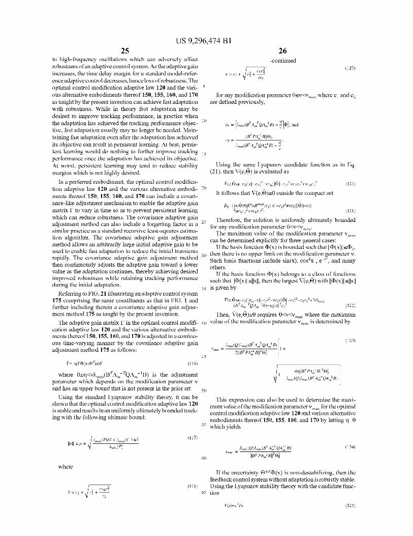
US 9,296,474 B1 25

to high-frequency oscillations which can adversely affect robustness of an adaptive control system. As the adaptive gain increases, the time delay margin for a standard model-refer-ence adaptive control decreases, hence loss ofrobustness. The optimal control modification adaptive law 120 and the vari-ous alternative embodiments thereof 150, 155, 160, and 170 as taught by the present invention can achieve fast adaptation with robustness. While in theory fast adaptation may be desired to improve tracking performance, in practice when the adaptation has achieved the tracking performance objec-tive, fast adaptation usually may no longer be needed. Main-taining fast adaptation even after the adaptation has achieved its objective can result in persistent learning. At best, persis-tent learning would do nothing to further improve tracking performance once the adaptation has achieved its objective. At worst, persistent learning may tend to reduce stability margins which is not highly desired.

In a preferred embodiment, the optimal control modifica-tion adaptive law 120 and the various alternative embodi-ments thereof 150, 155, 160, and 170 can include a covari-ance-like adjustment mechanism to enable the adaptive gain matrix E to vary in time so as to prevent persistent learning which can reduce robustness. The covariance adaptive gain adjustment method can also include a forgetting factor in a similar practice as a standard recursive least-squares estima-tion algorithm. The covariance adaptive gain adjustment method allows an arbitrarily large initial adaptive gain to be used to enable fast adaptation to reduce the initial transients rapidly. The covariance adaptive gain adjustment method then continuously adjusts the adaptive gain toward a lower value as the adaptation continues, thereby achieving desired improved robustness while retaining tracking performance during the initial adaptation.

Referring to FIG. 21 illustrating an adaptive control system 175 comprising the same constituents as that in FIG. 1 and further including therein a covariance adaptive gain adjust-ment method 175 as taught by the present invention.

The adaptive gain matrix E in the optimal control modifi-cation adaptive law 120 and the various alternative embodi-ments thereof 150, 155, 160, and 170 is adjusted in a continu-ous time-varying manner by the covariance adaptive gain adjustment method 175 as follows:

f--qF(D(x)(D T(x)F (116)

where 0:5rl<vX_ i„ (B TA_-TQAm-1 B) is the adjustment parameter which depends on the modification parameter v and has an upper bound that is not present in the prior art.

Using the standard Lyapunov stability theory, it can be shown that the optimal control modification adaptive law 120 is stable and results in an uniformly ultimately bounded track-ing with the following ultimate bound:

~m_(P)62 + Am_(~ 1)K2 (117)

Ilell P = Ami'(P)

where

(11 s) VC6C,

s=c2+FC2

C 1

26 -continued

K = C~ + C22 + c1 2

z (119)

VC6

for any modification parameter 0:5v<vmaz where c 1 and c z are defined previously,

10

C6 = [A,,,;a(BT A mT QA_'B) - ' I ],Do , and

JIB T PAm 1 BIIDo

A,,,;a (BT AmT QA M-1 B) - 77

15

Using the same Lyapunov candidate function as in Eq. (21), then V(e,0) is evaluated as

V(e,O)s-c i (lel-cz)'-vc60 0 -cl)'+c1 cz'+vc6c7' (120) 20

It follows that V(e,0)<_0 outside the compact set

Bb ((e,O)ER'xR °"P:c 1 (lel-c2)'+vc6(IIOI-c7) 2, J C22+vc6c72 ] (121)

25 Therefore, the solution is uniformly ultimately bounded for any modification parameter 0<v<vmaz.

The maximum value of the modification parameter v m_ can be determined explicitly for three general cases:

If the basis function (D(x) is bounded such that 114)(x)11<4) 0 ,

30 then there is no upper limit on the modification parameter v. Such basis functions include sin(x), cosy , e :

~2, and many

others. If the basis function (D(x) belongs to a class of functions

such that J(D(x)JJ`JJxJJ, then the largest V(e,0) with II (D(x)11:5 11xll 35 is given by

1- 411IIBT PAm1 BII202 A,,,;a (Q)A,,,;a (BT AmT

QAm1 B)

50

This expression can also be used to determine the maxi-mum value of the modification parameter v_ for the optimal control modification adaptive law 120 and various alternative embodiments thereof 150, 155, 160, and 170 by letting r) -0

55 which yields

A,,,;a (Q)A,,,;a (B T AmT QA M1 B) (124) vmax =

60 IIBTPAm1B11200

If the uncertainty O* T(D(x) is non-destabilizing, then the feedback control system without adaptation is robustly stable. Using the Lyapunov stability theory with the candidate func-

65 tion

V(e, 6)s- c1(I xl-c2)

2-vc6(IIDII-c7)2+c1c22+[Vk_i,

(B TAm TQAm 1B)— q]Ixl ~2 c72 (122)

Then, V(e,0):50 requires 0<v<vm_ where the maximum

40 value of the modification parameter v m_ is determined by

(123)

Um~

- Am;n (Q)A,,,;a (BT AmT QAm 1 B) 1 + 2 IIBT PAm1BII202

45

V(e)-e TPe (125)

US 9,296,474 B1 27

V(e):50 implies

II(D(x)11 < A ;a(Q)llell -2A._(P)wo (126)

211PBIIOo

Then, the largest V(e,0)is given by

V (e, 0) :~ - e1(Ilxm - XI I - e2) 2 - ve6(11011 - c7)2 + (127)

cici +[v;L i,(BTA-T QAm1 B) -17]A,,,;a(Q)llell-2;Lm-(P)wo c2

211PBIIOo

28 is referred herein to as the covariance adaptive gain adjust-ment method 185 and is described by

f—PF-gF(D(x) (D T(x)T (132)

5 where P -P T>0 is the forgetting factor matrix. Yet in another alternative embodiment, the covariance

adaptive gain adjustment method 185 includes a normaliza-tion factor which can also be used to change the time-varying rate of the adaptive gain matrix F(t). This alternative embodi-

10 ment is referred herein to as the covariance adaptive gain adjustment method 190 and is described by

C=/f- T 11 F(D(x)(D

T (x) F (133)

The maximum value of the modification parameter v_ is 15 1 + (D (x)R(D(x)

then determined to be With a forgetting factor, the adaptive gain matrix F(t) can

grow without bound. This can lead to poor robustness and (128) 20 may not improve performance. Therefore, a projection

method can be used to limit the effect of the forgetting factor. The projection method for the covariance adaptive gain adjustment method 185 is given by

2;Lmi,(BT AmT QAm1 B)11 PB11 2 vm~ _

;Lmi, (Q)II BT PAm1 B11 2

i7Am;a(Q)11 BT PAm 1 B11 2 1+ 1-Am

2;n(BTAmTQAm1B)IIPB112

This expression can also be used to determine the maxi-mum value of the modification parameter v_ for the optimal control modification adaptive law 120 and various alternative embodiments thereof 150, 155, 160, and 170 by letting q -0 which yields

4A», (BT AmT QAm 1 B)IIPB112 (129) vmax =

Ami,(Q)11 BT PAm1 B11 2

The covariance adaptive gain adjustment 175 generally causes the adaptive gain matrix F(t) to decrease uniformly from some initial values to small equilibrium values. In an alternative embodiment, the adjustment parameter rl is a matrix whose elements are the adjustment parameters for each individual element of the adaptive gain matrix. These adjustment parameters can be selectively chosen to change the time-varying rates of the individual elements of the adap-tive gain matrix F(t). The stability condition for the matrix of the adjustment parameters to be satisfied is

>vm_(q)<vkm,n(B TAm TQAm 1B) (130)

In another preferred embodiment, the covariance adaptive gain adjustment method 175 includes a normalization factor which can also be used to change the time-varying rate of the adaptive gain matrix F(t). This alternative embodiment is referred herein to as the covariance adaptive gain adjustment method 180 and is described by

25

1 L8F-r7C(D(x)(DT (x)C], if C;i _ Fii(to) (134)

CV - 1 l 0 otherwise

and the projection method for the covariance adaptive gain 3o adjustment method 190 is given by

i7C(D(x)(DT(x)C (135) /3C - T if C ;~ ~ C ;~(to)

35 w = 1 + ~ (x)R(D(x) ..

0 otherwise

The effects of the covariance adaptive gain adjustment method 175 and the alternative embodiment thereof 180 is to

40 gradually shut down the adaptation process. The effects of persistent learning and fast adaptation are therefore elimi-nated. A problem associated with the covariance adaptive gain adjustment methods 175 and 180 is that, once the adap-

45 tive gain matrix F(t) is reduced to an equilibrium value near zero, the adaptation process has to be restarted if a new uncertainty becomes present. Thus, in an alternative embodi-ment, the covariance adaptive gain adjustment methods 175 and 180 are used in conjunction with a resetting mechanism

50 195. The adaptation process can be reset with a new initial value of the adaptive gain to restart the covariance adaptive gain adjustment methods 175 and 180 whenever a threshold criterion is satisfied. The resetting mechanism 195 is expressed as

55

C = (136)

C with F(ti ) = [ ; t ? ti when threshold is exceeded at t = ti

C = - F (D(x)(DT (x) F

(131) C with C(0) = [ o otherwise

1 +(DT (x)R(D(x) 60

where R=RT>0 is a positive-definite normalization matrix. Yet in another alternative embodiment, the covariant adap-

tive gain adjustment method 175 can include a forgetting factor which can also be used to change the time-varying rate of the adaptive gain matrix F(t.) This alternative embodiment

where F, is a properly chosen new initial condition for the covariance adaptive gain adjustment methods 175 and 180 for t2A, when a new uncertainty becomes present.

65 The threshold should be chosen judiciously so that the trigger would occur appropriately to prevent false triggering. Also when a switching action occurs with a large change in

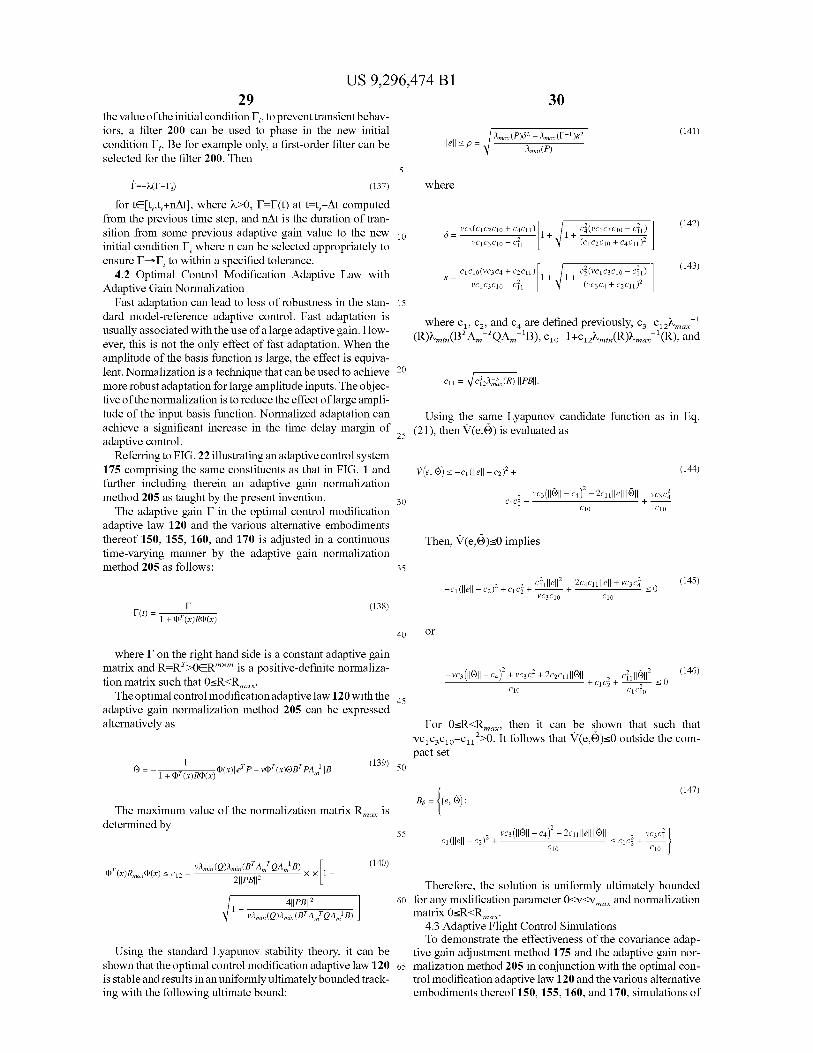
US 9,296,474 B1 29 30

the value of the initial condition F,, to prevent transientbehav-

iors, a filter 200 can be used to phase in the new initial ~ (P)~z +~ _ ([-1 )K2

condition F , . Be for example only, a first-order filter can be Ilell <P = .n(P)

selected for the filter 200. Then 5

f (F—I',) (137) where

(141)

(142)

(143)

for tE[t,,t,+nAt], where X>O, F=F(t) at t=t,-At computed from the previous time step, and nAt is the duration of tran-sition from some previous adaptive gain value to the new initial condition F, where n can be selected appropriately to ensure F—F, to within a specified tolerance.

4.2 Optimal Control Modification Adaptive Law with Adaptive Gain Normalization

Fast adaptation can lead to loss of robustness in the stan-dard model-reference adaptive control. Fast adaptation is usually associated with the use of a large adaptive gain. How-ever, this is not the only effect of fast adaptation. When the amplitude of the basis function is large, the effect is equiva-lent. Normalization is a technique that can be used to achieve more robust adaptation for large amplitude inputs. The objec-tive of the normalization is to reduce the effect of large ampli-tude of the input basis function. Normalized adaptation can achieve a significant increase in the time delay margin of adaptive control.

Referring to FIG. 22 illustrating an adaptive control system 175 comprising the same constituents as that in FIG. 1 and further including therein an adaptive gain normalization method 205 as taught by the present invention.

The adaptive gain F in the optimal control modification adaptive law 120 and the various alternative embodiments thereof 150, 155, 160, and 170 is adjusted in a continuous time-varying manner by the adaptive gain normalization method 205 as follows:

C (138) C(t) =

1+(DT(x)R$(x)

Vc3 (C1C2C10 + C4C11) ~1 C2(VC 1 C3C10 — C11)

10 -

vc1C3C10 — Ci1 (C1C2C10 + C4C11)2

K— C1C10(VC3c4 + C2C11) ~ 1 + 1+ Cz(VCtC3C10 — C21)

VC1C3C10 — C1 (VC3C4 + C2C11 )2

15

where c l , c2, and c4 are defined previously, c3_C12X 1

(R)Xm=n(B TAm-TQAm

-1B), C10 1 +c12Xm,n(R)Xma 1 (R), and

20

Ctt =C12~,»"(R) IIPBII.

Using the same Lyapunov candidate function as in Eq. 25 (21), then V(e,0) is evaluated as

V (e, 0) <- — ci (Ilell - C2)2 + (144)

2 VC3 (11011 — C4)2 — 2c1111e1111011 vc3 c2 30 c1 c2 — +

C10 C10

Then, V(e,0):50 implies

35

z z Ci1e12 ZC4C11e+vc3c4 (145) — Ct(Ilell — c2) +c1 c2+ + 1- 0

VC3C10 C10

40 or

where F on the right hand side is a constant adaptive gain matrix and R=RT>OERm"m is a positive-definite normaliza-

vc3 c4) + vc3 c4 + 2czc1111 011 z 2 2 2 (146)

- (11011 — tion matrix such that 0<-R<Rm,, . +C,C2 +

c 11 011 11 CtC

2 <_ 010

The optimal control modification adaptive law 120 with the 45 Cto

adaptive gain normalization method 205 can be expressed alternatively as For 0:5R<Rmax, then it can be shown that such that

vc1C3C10-0112>0. It follows that V(e,0):50 outside the com-pact set

0=— (D (x)[eTP — V(DT(x)OBTPAm1]B (13

+ 9) 50

1 (DT (x) R~(x)

(147)

The maximum value of the normalization matrix R__ is determined by

T VA,,,;a(Q)A,,,;a(BTAmTQAm1B) (140)

(x)Rmax~ (x) C1z = 211PB112

x x 1 +

411PB11 2 vAmia (Q)Am;, (BT AmT QAm 1 B)

Using the standard Lyapunov stability theory, it can be shown that the optimal control modification adaptive law 120 is stable and results in an uniformly ultimately bounded track-ing with the following ultimate bound:

55 ct (Ilell — C2) 2 +

VC3 (11011 — C4)2 —

2c11 11e1111011 < C1C2 + VC3C4

C10 C10

Therefore, the solution is uniformly ultimately bounded 60 for any modification parameter 0<v<vmaz and normalization

matrix 0:5R<Rma 4.3 Adaptive Flight Control Simulations To demonstrate the effectiveness of the covariance adap-

tive gain adjustment method 175 and the adaptive gain nor- 65 malization method 205 in conjunction with the optimal con-

trol modification adaptive law 120 and the various alternative embodiments thereof 150, 155, 160, and 170, simulations of

1+

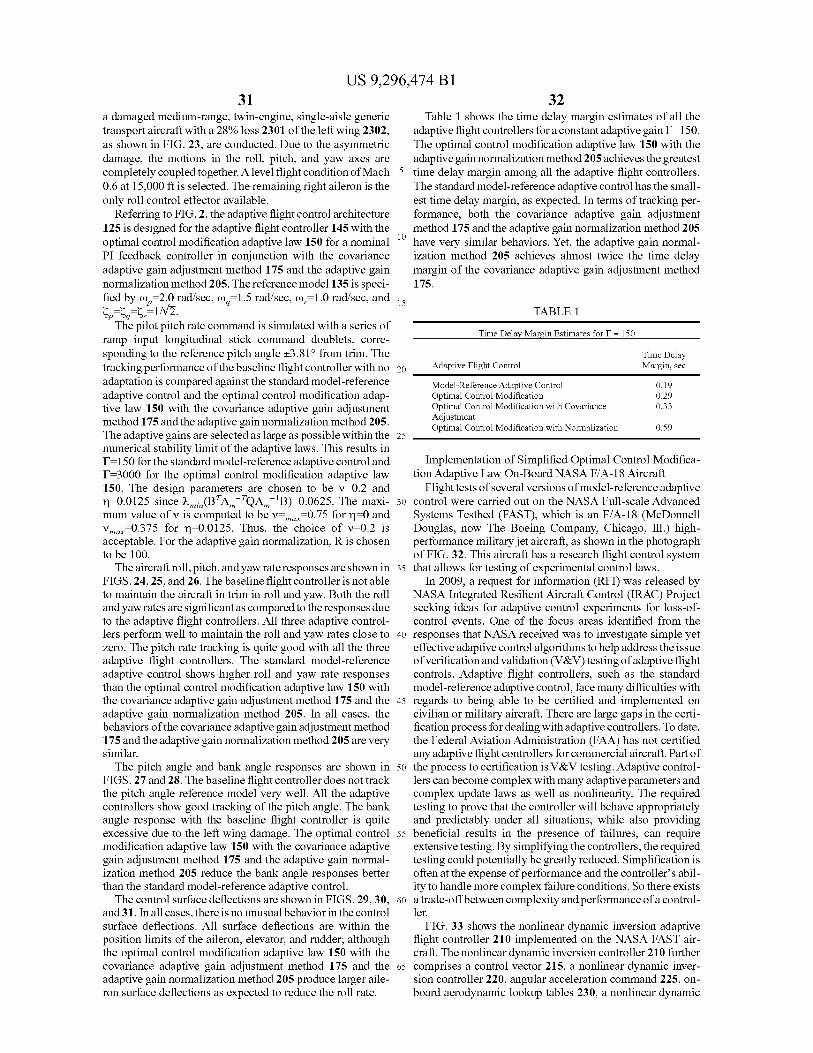
US 9,296,474 B1 31

a damaged medium-range, twin-engine, single-aisle generic transport aircraft with a 28% loss 2301 of the left wing 2302, as shown in FIG. 23, are conducted. Due to the asymmetric damage, the motions in the roll, pitch, and yaw axes are completely coupled together. A level flight condition of Mach 0.6 at 15,000 ft is selected. The remaining right aileron is the only roll control effector available.

Referring to FIG. 2, the adaptive flight control architecture 125 is designed for the adaptive flight controller 145 with the optimal control modification adaptive law 150 for a nominal PI feedback controller in conjunction with the covariance adaptive gain adjustment method 175 and the adaptive gain normalization method 205. The reference model 135 is speci-fied by wP=2.0 rad/sec, w. — I.5 rad/sec, w, 1.0 rad/sec, and

~P ~q ~r 1/✓2. The pilot pitch rate command is simulated with a series of

ramp input longitudinal stick command doublets, corre-sponding to the reference pitch angle t3.81' from trim. The tracking performance of the baseline flight controller with no adaptation is compared against the standard model-reference adaptive control and the optimal control modification adap-tive law 150 with the covariance adaptive gain adjustment method 175 and the adaptive gain normalization method 205. The adaptive gains are selected as large as possible within the numerical stability limit of the adaptive laws. This results in E=150 for the standard model-reference adaptive control and E=3000 for the optimal control modification adaptive law 150. The design parameters are chosen to be v -0.2 and r1 -0.0125 since X_ i„(B TA_-TQAm- 'B)-0.0625. The maxi-mum value of v is computed to be v= m,,-0.75 for fl -0 and vm_-0.375 for r1 -0.0125. Thus, the choice of v-0.2 is acceptable. For the adaptive gain normalization, R is chosen to be 100.

The aircraft roll, pitch, and yaw rate responses are shown in FIGS. 24, 25, and 26. The baseline flight controller is not able to maintain the aircraft in trim in roll and yaw. Both the roll and yaw rates are significant as compared to the responses due to the adaptive flight controllers. All three adaptive control-lers perform well to maintain the roll and yaw rates close to zero. The pitch rate tracking is quite good with all the three adaptive flight controllers. The standard model-reference adaptive control shows higher roll and yaw rate responses than the optimal control modification adaptive law 150 with the covariance adaptive gain adjustment method 175 and the adaptive gain normalization method 205. In all cases, the behaviors of the covariance adaptive gain adjustment method 175 and the adaptive gain normalization method 205 are very similar.

The pitch angle and bank angle responses are shown in FIGS. 27 and 28. The baseline flight controller does not track the pitch angle reference model very well. All the adaptive controllers show good tracking of the pitch angle. The bank angle response with the baseline flight controller is quite excessive due to the left wing damage. The optimal control modification adaptive law 150 with the covariance adaptive gain adjustment method 175 and the adaptive gain normal-ization method 205 reduce the bank angle responses better than the standard model-reference adaptive control.

The control surface deflections are shown in FIGS. 29, 30, and 31. In all cases, there is no unusual behavior in the control surface deflections. All surface deflections are within the position limits of the aileron, elevator, and rudder; although the optimal control modification adaptive law 150 with the covariance adaptive gain adjustment method 175 and the adaptive gain normalization method 205 produce larger aile-ron surface deflections as expected to reduce the roll rate.

32 Table 1 shows the time delay margin estimates of all the

adaptive flight controllers for a constant adaptive gain E=150. The optimal control modification adaptive law 150 with the adaptive gain normalization method 205 achieves the greatest

5 time delay margin among all the adaptive flight controllers. The standard model-reference adaptive control has the small-est time delay margin, as expected. In terms of tracking per-formance, both the covariance adaptive gain adjustment method 175 and the adaptive gain normalization method 205

to have very similar behaviors. Yet, the adaptive gain normal-ization method 205 achieves almost twice the time delay margin of the covariance adaptive gain adjustment method 175.

15 TABLE 1

Time Delay Margin Estimates for F = 150

Time Delay

20 Adaptive Flight Control Margin, sec

Model-Reference Adaptive Control 0.19 Optimal Control Modification 0.29 Optimal Control Modification with Covariance 0.33 Adjustment Optimal Control Modification with Normalization 0.59

25

Implementation of Simplified Optimal Control Modifica-tion Adaptive Law On-Board NASA F/A-18 Aircraft

Flight tests of several versions of model-reference adaptive 30 control were carried out on the NASA Full-scale Advanced

Systems Testbed (FAST), which is an F/A-18 (McDonnell Douglas, now The Boeing Company, Chicago, Ill.) high-performance military j et aircraft, as shown in the photograph of FIG. 32. This aircraft has a research flight control system

35 that allows for testing of experimental control laws. In 2009, a request for information (RFI) was released by

NASA Integrated Resilient Aircraft Control (IRAQ Project seeking ideas for adaptive control experiments for loss-of-control events. One of the focus areas identified from the

4o responses that NASA received was to investigate simple yet effective adaptive control algorithms to help address the issue of verification and validation (V&V) testing of adaptive flight controls. Adaptive flight controllers, such as the standard model-reference adaptive control, face many difficulties with

45 regards to being able to be certified and implemented on civilian or military aircraft. There are large gaps in the certi-fication process for dealing with adaptive controllers. To date, the Federal Aviation Administration (FAA) has not certified any adaptive flight controllers for commercial aircraft. Part of

50 the process to certification is V&V testing. Adaptive control-lers can become complex with many adaptive parameters and complex update laws as well as nonlinearity. The required testing to prove that the controller will behave appropriately and predictably under all situations, while also providing

55 beneficial results in the presence of failures, can require extensive testing. By simplifying the controllers, the required testing could potentially be greatly reduced. Simplification is often at the expense of performance and the controller's abil-ity to handle more complex failure conditions. So there exists

6o a trade-off between complexity and performance of a control-ler.

FIG. 33 shows the nonlinear dynamic inversion adaptive flight controller 210 implemented on the NASA FAST aircraft. The nonlinear dynamic inversion controller 210 further

65 comprises a control vector 215, a nonlinear dynamic inversion controller 220, angular acceleration command 225, on- board aerodynamic lookup tables 230, a nonlinear dynamic

US 9,296,474 B1 33 34

inversion reference model 235, an adaptive control reference The pilot commands 270 rp (t) and rq(t) are computed from

model 240, an error compensator 245, an adaptive augmen- the pilot stick inputs 6,,,(t) and 6,,,(t) according to tation controller 250 employing three adaptive laws 255, 260, and 265, a pilot command 270, and a plant 275 which is the NASA FAST aircraft. 5 Y (153)

r ~ ~~kp cop ~tar

The control vector 215 has ten control surface commands, a

denoted as 6, and is computed by the nonlinear dynamic Yg kgwg[6,o„+c~~~mn dr1 inversion controller 220 as °

6=B,- '[Y_,+ Q xIQ f,(y)]+6 o (148) 10 The error compensator 245 is necessary to improve track-

where the vector of estimated aerodynamic moments fA(y) ing of the reference model in the presence of model uncer-

is calculated from the on-board aerodynamic lookup tables tainty and disturbances by the nonlinear dynamic inversion

230, while the angular rates Q are measured using aircraft controller 220 without adaptive augmentation. The nonlinear

sensors, I is the inertia matrix of the aircraft, 6,, are pre- 15 dynamic inversion controller 220 in the pitch axis contains a

determined trim surface commands appropriate for the test proportional-integral (PI) error compensator. The nonlinear

flight condition, and B,- ' is a weighted pseudo-inverse of the dynamic inversion controller 220 in the roll axis contains a

control effectiveness derivatives with respect to the surface proportional error compensator. The gains of the error com-

positions weighted by a control allocation matrix. pensator 245 are tuned to match the adaptive control refer-

The weighted pseudo-inverse B, - ' is computed as follows: 20 ence model 240. Thus

B,- ' - ff-'B, T(B,ff-'B, T) - ' (149)

P~ cop(P.f - P) (154)

The angular acceleration commands Xc_ jt) contain the g = 2Sa ~a(i r g) +

~~ ((g r g)

~~

sum of the desired reference dynamics X,, t(t) produced by the 25 J0 nonlinear dynamic inversion reference model 235, the output Xc jt) of the error compensator 245, and adaptive control aug-

mentation Yc jt) computed by the adaptive augmentation con- The aircraft's true, unknown dynamics are written as

troller 250. This is described as

30 z=Ax +Bm (u-a) (155)

or

P,f + P, + P p (150)

g,f+g,+g,

_(0)

p +Bp) 1 0 (156) Y,f+r

P

35 9 - 0 0 1

R 0-( p +egt ) - (2Spo)p +9gz )

Note that the adaptive controller only augments the pitch and roll axes. P 1 0

The nonlinear dynamic inversion reference model 235 for 40 ~ g dT + 0 0

the adaptive control reference model 240 each are by the pilot ° 0 1 ug

- O-g

command 270 r(t). The nonlinear dynamic inversion refer- g

ence model 235 generally represents the same desired

dynamics as the adaptive control reference model 240, but where 6P, 0,,, and 6 q2 the uncertain parameters; and 6P (t) may be modified to simulate a failed or damaged aircraft. The 45 and 6q(t) are scalar, time-varying uncertain disturbances.

state feedback vector y(t) contains measurements of the The nonlinear dynamic inversion adaptive flight controller

inputs required for the aerodynamic lookup tables 230, such 210 is then designed to cancel out the effects of the uncertain

as angle of attack and velocity, as well as the angular rates. parameters 6P, 0q , 1 6q2, 6P (t), and 6q(t) by the adaptive aug-

The adaptive control reference model 240 for the aircraft mentation controller 250. This is expressed as axis of interest is specified as a stable, linear time-invariant 50 system as

up rp + Pp (157)

zm =Amxm +Bmr (151) ug - Y p + qp

or

55

where

Pm -cop 1 0 Pm 1 0

(~

do

lII Yp

im = 0 0 1 J im(T)d1T O

JY

~ yy L 9 gm 0

_(,)2g -20 W9

0 1

Qm

(152)

B,P + &p (158)

60 Pa _ (~

9gi Jgdr+9gzg+&g

0

The pitch axis reference model is second order, represent- 5.1 Simple Model-Reference Adaptive Control ing the desired short-period dynamics. The roll axis reference 65 In one embodiment, the adaptive augmentation controller model is first order, and no adaptive augmentation is applied 250 employs a simple model-reference adaptive control 255, in the yaw axis. designated as sMRAC adaptive lazes. The sMRAC adaptive

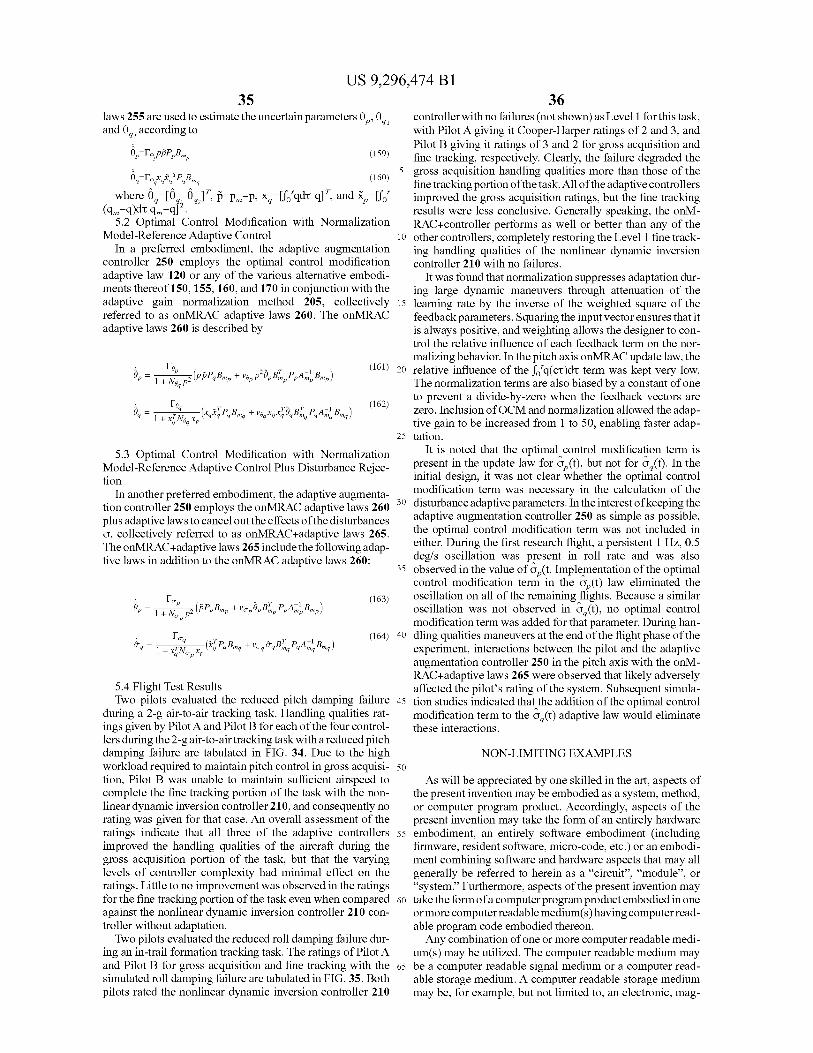
US 9,296,474 B1 35

laws 255 are used to estimate the uncertain parameters 0 1, 01, and 0., according to

6P ra,pPP,BmP (159)

0g F.,xsR,'PgB_, (160) Where 6,_ [6 q 6 g2] r, p=p--p, xq [Utgdti q]T and XP=Uot

(qm —q)& qm —q] f. 5.2 Optimal Control Modification with Normalization

Model-Reference Adaptive Control In a preferred embodiment, the adaptive augmentation

controller 250 employs the optimal control modification adaptive law 120 or any of the various alternative embodi-ments thereof 150,155, 160, and 170 in conjunction with the adaptive gain normalization method 205 , collectively referred to as onMRAC adaptive laws 260. The onMRAC adaptive laws 260 is described by

0, dap 21pppaBmp+v,,P2B,BmpPpAmpBmp)

(161)

1 + Naq p

8q = 7,e9

(X j pq Bmq + Vqq xq xq B9Bmq

pq Am'

Bm9) (162)

1+xq N,g xp

5.3 Optimal Control Modification with Normalization Model-Reference Adaptive Control Plus Disturbance Rejec-tion

In another preferred embodiment, the adaptive augmenta-tion controller 250 employs the onMRAC adaptive laws 260 plus adaptive laws to cancel outthe effects ofthe disturbances u, collectively referred to as onMRAC+adaptive laws 265. The onMRAC+adaptive laws 265 include the following adap-tive laws in addition to the onMRAC adaptive laws 260:

C, / (163) 0, 1 +Nip p2 (PP Bmp +VQp

Bp Bmp pp A

-1 Bmp/

CI / (164) ~q 1+xTN~ x lxapaBmg+v~q 5 gBmgPqAmgBmq

~ 9 p p

5.4 Flight Test Results Two pilots evaluated the reduced pitch damping failure

during a 2-g air-to -air tracking task. Handling qualities rat-ings given by Pilot A and Pilot B for each of the four control-lers during the 2-g air-to-air tracking task with a reduced pitch damping failure are tabulated in FIG. 34. Due to the high workload required to maintain pitch control in gross acquisi-tion, Pilot B was unable to maintain sufficient airspeed to complete the fine tracking portion of the task with the non-linear dynamic inversion controller 210, and consequently no rating was given for that case. An overall assessment of the ratings indicate that all three of the adaptive controllers improved the handling qualities of the aircraft during the gross acquisition portion of the task, but that the varying levels of controller complexity had minimal effect on the ratings. Little to no improvement was observed in the ratings for the fine tracking portion of the task even when compared against the nonlinear dynamic inversion controller 210 con-troller without adaptation.

Two pilots evaluated the reduced roll damping failure dur-ing an in-trail formation tracking task. The ratings of Pilot A and Pilot B for gross acquisition and fine tracking with the simulated roll damping failure are tabulated in FIG. 35. Both pilots rated the nonlinear dynamic inversion controller 210

36 controller with no failures (not shown) as Level I for this task, with Pilot A giving it Cooper-Harper ratings of 2 and 3, and Pilot B giving it ratings of 3 and 2 for gross acquisition and fine tracking, respectively. Clearly, the failure degraded the

5 gross acquisition handling qualities more than those of the fine tracking portion of the task. All of the adaptive controllers improved the gross acquisition ratings, but the fine tracking results were less conclusive . Generally speaking, the onM-RAC+controller performs as well or better than any of the

10 other controllers, completely restoring the Level I fine track-ing handling qualities of the nonlinear dynamic inversion controller 210 with no failures.

It was found that normalization suppresses adaptation dur-ing large dynamic maneuvers through attenuation of the

15 learning rate by the inverse of the weighted square of the feedback parameters . Squaring the input vector ensures that it is always positive , and weighting allows the designer to con-trol the relative influence of each feedback term on the nor-malizing behavior. In the pitch axis onMRAC update law, the

20 relative influence of the fotq(ct)dti term was kept very low. The normalization terms are also biased by a constant of one to prevent a divide-by-zero when the feedback vectors are zero. Inclusion of OCM and normalization allowed the adap-tive gain to be increased from I to 50, enabling faster adap-

25 tation. It is noted that the optimal control modification term is

present in the update law for 6P (t), but not for 6g(t). In the initial design, it was not clear whether the optimal control modification term was necessary in the calculation of the

30 disturbance adaptive parameters. In the interest of keeping the adaptive augmentation controller 250 as simple as possible, the optimal control modification term was not included in either. During the first research flight, a persistent I Hz, 0.5 deg/s oscillation was present in roll rate and was also

35 observed in the value of ap(t. Implementation of the optimal control modification term in the 6P (t) law eliminated the oscillation on all of the remaining flights. Because a similar oscillation was not observed in 6g(t), no optimal control modification term was added for that parameter. During han-

40 dling qualities maneuvers at the end of the flight phase of the experiment, interactions between the pilot and the adaptive augmentation controller 250 in the pitch axis with the onM-RAC+adaptive laws 265 were observed that likely adversely affected the pilot's rating of the system. Subsequent simula-

45 tion studies indicated that the addition of the optimal control modification term to the 6g(t) adaptive law would eliminate these interactions.

NON-LIMITING EXAMPLES 50

As will be appreciated by one skilled in the art, aspects of the present invention may be embodied as a system, method, or computer program product . Accordingly, aspects of the present invention may take the form of an entirely hardware

55 embodiment , an entirely software embodiment (including firmware, resident software , micro-code, etc .) or an embodi-ment combining software and hardware aspects that may all generally be referred to herein as a "circuit", "module", or "system." Furthermore, aspects of the present invention may

60 take the form of a computer program product embodied in one or more computer readable medium(s) having computer read-able program code embodied thereon.

Any combination of one or more computer readable medium(s) may be utilized. The computer readable medium may

65 be a computer readable signal medium or a computer readable storage medium. A computer readable storage medium may be, for example, but not limited to, an electronic, mag-

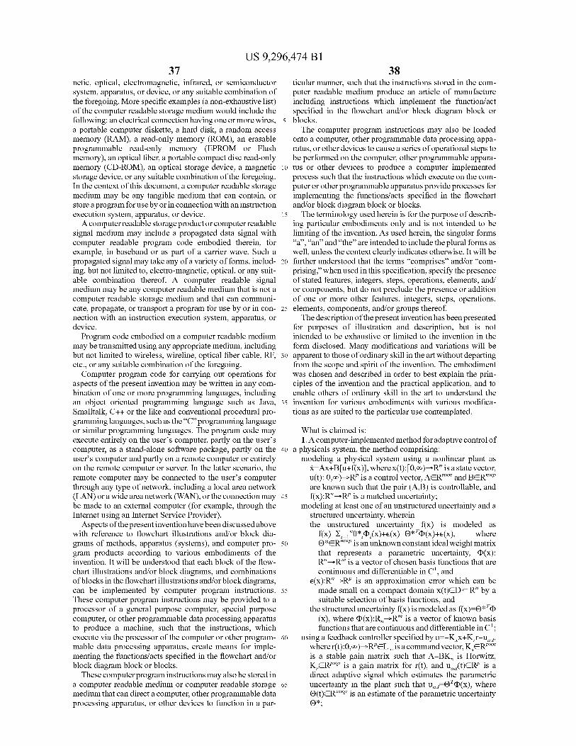
US 9,296,474 B1 37

38 netic, optical, electromagnetic, infrared, or semiconductor ticular manner, such that the instructions stored in the com- system, apparatus, or device, or any suitable combination of

puter readable medium produce an article of manufacture

the foregoing. More specific examples (a non-exhaustive list)

including instructions which implement the function/act of the computer readable storage medium would include the specified in the flowchart and/or block diagram block or following: an electrical connection having one or more wires, 5 blocks. a portable computer diskette, a hard disk, a random access

The computer program instructions may also be loaded

memory (RAM), a read-only memory (ROM), an erasable onto a computer, other programmable data processing appa- programmable read-only memory (EPROM or Flash

ratus, or other devices to cause a series of operational steps to

memory), an optical fiber, a portable compact disc read-only

be performed on the computer, other programmable appara- memory (CD-ROM), an optical storage device, a magnetic io tus or other devices to produce a computer implemented storage device, or any suitable combination of the foregoing. process such that the instructions which execute on the com- In the context of this document, a computer readable storage puter or other programmable apparatus provide processes for medium may be any tangible medium that can contain, or

implementing the functions/acts specified in the flowchart

store a program for use by or in connection with an instruction and/or block diagram block or blocks. execution system, apparatus, or device. 15 The terminology used herein is for the purpose of describ-

A computer readable storage product or computer readable

ing particular embodiments only and is not intended to be signal medium may include a propagated data signal with

limiting of the invention. As used herein, the singular forms

computer readable program code embodied therein, for

"a", "an" and "the" are intended to include the plural forms as example, in baseband or as part of a carrier wave. Such a well, unless the context clearly indicates otherwise. It will be propagated signal may take any of a variety of forms, includ- 20 further understood that the terms "comprises" and/or "com- ing, but not limited to, electro-magnetic, optical, or any suit- pri sing," when used in this specification, specify the presence able combination thereof. A computer readable signal

of stated features, integers, steps, operations, elements, and/

medium may be any computer readable medium that is not a or components, but do not preclude the presence or addition computer readable storage medium and that can communi- of one or more other features, integers, steps, operations, cate, propagate, or transport a program for use by or in con- 25 elements, components, and/or groups thereof. nection with an instruction execution system, apparatus, or

The description of the present invention has been presented

device. for purposes of illustration and description, but is not Program code embodied on a computer readable medium

intended to be exhaustive or limited to the invention in the

may be transmitted using any appropriate medium, including

form disclosed. Many modifications and variations will be but not limited to wireless, wireline, optical fiber cable, RF, so apparent to those of ordinary skill in the art without departing etc., or any suitable combination of the foregoing. from the scope and spirit of the invention. The embodiment

Computer program code for carrying out operations for was chosen and described in order to best explain the prin- aspects of the present invention may be written in any com- ciples of the invention and the practical application, and to bination of one or more programming languages, including enable others of ordinary skill in the art to understand the an object oriented programming language such as Java, 35 invention for various embodiments with various modifica-Smalltalk, C++ or the like and conventional procedural pro- tions as are suited to the particular use contemplated. gramming languages, such as the "C" programming language or similar programming languages. The program code may

What is claimed is:

execute entirely on the user's computer, partly on the user's

1. A computer-implemented method for adaptive control of computer, as a stand-alone software package, partly on the 4o a physicals system, the method comprising: user's computer and partly on a remote computer or entirely modeling a physical system using a nonlinear plant as on the remote computer or server. In the latter scenario, the

X=Ax+B[u+f(x)], wherex(t): [0,-)—R" is a state vector,

remote computer may be connected to the user's computer u(t): 0,-)—RP is a control vector, AER""" and BER"" P

through any type of network, including a local area network

are known such that the pair (A,B) is controllable, and (LAN) or a wide area network (WAN), or the connection may 45 f(x):R"—RP is a matched uncertainty; be made to an external computer (for example, through the modeling at least one of an unstructured uncertainty and a Internet using an Internet Service Provider). structured uncertainty, wherein

Aspects of the present invention have been discussed above the unstructured uncertainty f(x) is modeled as with reference to flowchart illustrations and/or block dia- f(x)=E,_i"O*,4){x)+e(x)=0* T(D(x)+e(x), where grams of methods, apparatus (systems), and computer pro- 50 O*ER- Pisanunknownconstantidealweightmatrix gram products according to various embodiments of the that represents a parametric uncertainty, (D(x): invention. It will be understood that each block of the flow- R"—R'" is a vector of chosen basis functions that are chart illustrations and/or block diagrams, and combinations continuous and differentiable in C i , and of blocks in the flowchart illustrations and/or block diagrams, e(x):R"—RP is an approximation error which can be can be implemented by computer program instructions. 55 made small on a compact domain x(t)ED - R" by a These computer program instructions may be provided to a suitable selection of basis functions, and processor of a general purpose computer, special purpose the structured uncertainty f(x) is modeled as f(x)=0 * T(D computer, or other programmable data processing apparatus

(x), where (D(x):R"—R'" is a vector of known basis

to produce a machine, such that the instructions, which

functions that are continuous and differentiable in C i ; execute via the processor of the computer or other program- 60 using a feedback controller specified by a=—K xx+K r—u ad,

mable data processing apparatus, create means for imple- where r(t):0,-)—RPEL_ is a command vector, K xERP"" menting the functions/acts specified in the flowchart and/or

is a stable gain matrix such that A—BK, is Horwitz,

block diagram block or blocks. K,.ERP"P is a gain matrix for r(t), and a "d(t)ERP is a These computer program instructions may also be stored in

direct adaptive signal which estimates the parametric

a computer readable medium or computer readable storage 65 uncertainty in the plant such that uad OT(D(x), where medium that can direct a computer, other programmable data

O(t)ER"P is an estimate of the parametric uncertainty

processing apparatus, or other devices to function in a par- O*;

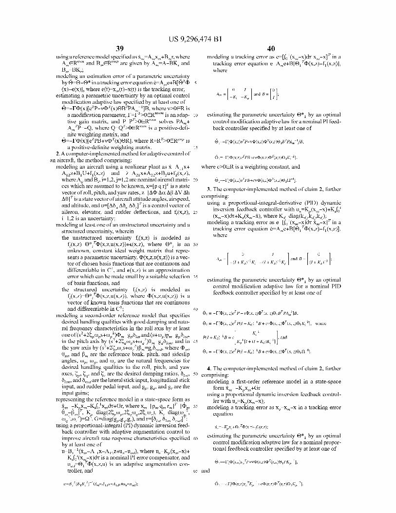
US 9,296,474 B1 39

using a reference model specified as X m=Amxm +Bmr, where AmER""" and B mER" P are given by Am=A-BKx and Bm=BK,.;

modeling an estimation error of a parametric uncertainty by 0=0-0 * in a tracking error equation e=A me+B [O T(D 5 (x)-e(x)], where e(t)=x m (t)-x(t) is the tracking error;

estimating a parametric uncertainty by an optimal control modification adaptive law specified by at least one of 6=-F(D(x)[eTP-v(D T(x)OB TPAm-1]B, where v>OER is

a modification parameter, F-FT>OER-'— is an adap- io tive gain matrix, and P=P T>OER""" solves PAm + Am TP=-Q, where Q=Q T>OER""" is a positive-definite weighting matrix, and

O=-F(D(x)[eTPB+v(D T(x)OR], where R=RT>OERP P is a positive-definite weighting matrix. 15

2. A computer-implemented method for adaptive control of an aircraft, the method comprising:

modeling an aircraft using a nonlinear plant as x=A 11x+ Al2z+B,U+fl (x,z) and 2=A21 x+A22z+B2u+f2(x,z), where Ali and B , , i=1,2, j=1,2 are nominal aircraft matri- 20 ces which are assumed to be known, x=[p q r] T is a state vector of roll, pitch, and yaw rates, z=[A(D Aa AR AV Ah AO] T is a state vector of aircraft attitude angles, airspeed, and altitude, and a=[Aria Ab e A6,.] T is a control vector of aileron, elevator, and rudder deflections, and f (X,z), 25 i=1,2 is an uncertainty;

modeling at least one of an unstructured uncertainty and a structured uncertainty, wherein the unstructured uncertainty f.(x,z) is modeled as

f.(x,z)=0*, T4)(x,z,u(x,z))+e(x,z), where O*, is an 30 unknown, constant ideal weight matrix that repre-sents a parametric uncertainty, (D(x,z,u(x,z)) is a vector of chosen basis functions that are continuous and differentiable in C l , and e(x,z) is an approximation error which can be made small by a suitable selection 35 of basis functions, and

the structured uncertainty f.(x,z) is modeled as f.(x,z)=0*, T4)(x,z,u(x,z)), where (D(x,z,u(x,z)) is a vector of known basis functions that are continuous and differentiable in C l ; 40

modeling a second-order reference model that specifies desired handling qualities with good damping and natu-ral frequency characteristics in the roll axis by at least one of(S 2 +2~rwP S +wP2)~ =gp6,,,and(s+wP)pm=gP6, , in the pitch axis by (S 2+2~gwgS+wg2)0 m=ggSio", and in 45 the yaw axis by (S2 +2~,,w,,s+w,,2)(3 m=g,.6,.ud, where (D m , O m, and P. are the reference bank, pitch, and sideslip angles, Cop , wq, and w,, are the natural frequencies for desired handling qualities in the roll, pitch, and yaw axes, ~P , ~q, and ~,, are the desired damping ratios, 6,, t, 50 6io", and 6,,"d are the lateral stick input, longitudinal stick input, and rudder pedal input, and gP , gq, and g,, are the input gains;

representing the reference model in a state-space form as xm=-KPxm-Kfo lxmd2+Gr, where xm=[pm qm rm]T[~ 55 6m2 ( m] g, K -diag(2~ cop,2~^,2~ ), K,-liag(w2 ,

wq ,wr )=SZ , G-liag(gplgglgr), and r=[6,,t bio" 6,."A using a proportional-integral (PI) dynamic inversion feed-

back controller with adaptive augmentation control to improve aircraft rate response characteristics specified 60 by at least one of u=B

1 -1 (Xm-Arrx-Al2z+ue-uad), where ue KP (xm-x)+ Kfot(xm -x)dti is a nominal PI error compensator, and uad O 1 T(D(x,z,u) is an adaptive augmentation con-troller, and 65

40 modeling a tracking error as e=Uo l (xm -x)dti xm -x] T in a

tracking error equation where

o i Am - ~

o -K; -K P

I andB= ~ 0 ~ ;

estimating the parametric uncertainty O * 1 by an optimal control modification adaptive law for a nominal PI feed-back controller specified by at least one of

Oi -F[(D(x,z)e TP-v(D(x,z)(D T(x,z)O,B TPAm ']B,

Oi -F[(D(x,z)e TPB+"(x,z)(D 7(x,z)O,Ks 2],

where c>OER is a weighting constant, and

Oi -F[(D(x,z)e 7PB+"(x,z)(D 7(x,z)O,Q -4].

3. The computer-implemented method of claim 2, further comprising:

using a proportional-integral-derivative (PID) dynamic inversion feedback controller with u e KP (xm-x)+Kfot (xm -x)dti+Kd(Xm -X), where Kd-liag(kd ,kd ,kd );

modeling a tracking error as e=[fo l (xm -x)& Xm -x] T in a tracking error equation e=A me+B[O 1 T~ (x,z)-f1 (x,z)], where

u i u Am = and B -

-(l + Kd)-i K; - (l + Kd)-i

KP (l + Kd )-i

estimating the parametric uncertainty O * 1 by an optimal control modification adaptive law for a nominal PID feedback controller specified by at least one of

Ot = - F[(D(x, Z)eT P - v(D(x, Z)(DT (x, Z)O,BT PAm1 IB,

01 = - F[(D(x, Z)eT py + Kd)- 'B + cv(D(x, Z)(DT (x, Z)Oi K; 2], where

K-t

MI + Kd)-i B = c and Kp i [I+(l+Kd )K; i ]

Ot = - F [(D(x, Z)eT py + Kd )-i B + cv(D(x, Z)(DT (x, Z)Ol n-4].


modeling a first-order reference model in a state-space form x_=-KPxm +Gr

using a proportional dynamic inversion feedback control-ler with ue KP (xm -x);

modeling a tracking error as x,=x m -x in a tracking error equation

z,--K Fx,+Oj T(D(x, z) fj(x,z);

estimating the parametric uncertainty O * 1 by an optimal control modification adaptive law for a nominal propor-tional feedback controller specified by at least one of

Oi -F[(D(x,z)x,'P+v(D(x,z)(D T(x,z)O,PKP i],

and

u=B, T(B,B, T) i (xm A iix-A l2z+ue u,d); 6 1 =-cF[(D(x,z)x,TKP i +v(D(x,z)(D T(x,z)O,KP 2].

US 9,296,474 B1 41

5. The computer-implemented methods of claim 1 , farther comprising:

accessing an adaptive gain matrix F allowed to be time-varying;

calculating, with a processor, optimal control modification adaptive laws with time-varying adaptive gain F(t);

using a covariance adaptive gain adjustment method described by at least one of

I --r1I)(x)41) T(x)F, where 0:5rl<vX_JB TA_-T QA_-1 B)ER is an adjustment parameter which depends on the modification parameter v, and 0 :5v<vm_ where v m_ has no limit if the basis function (D(x) is bounded such that J(D(x)11<4) 0 or

V.- =

Ami,(Q)Ami,(B T AmT QAm1B) ~1 + 1 — 41111BT PAm1 B11

10o

211BT PAm 1 B11 202 Ami,(Q)A a(BT AmT QAm1 B)

if the basis function (D(x) belongs to a class of functions such that J4)(x)JJ:5JJxJJ or

42

C with F(ti ) = [ ; t ? ti when threshold is exceeded at t = t;

C with C(0) = F O otherwise

where F, is a properly chosen new initial condition for the covariance adaptive gain adjustment method for t2A, when a new uncertainty becomes present , and F, is phased in by a first-order filter I=- ~ (I -I ~) or any order filter so chosen for

to tE[t,,t,+nAt], where X>O, F-F(t) as t=t,-At computed from the previous time step and nAt is the duration of transition from some previous adaptive gain value to the new initial condition F, where n can be selected appropriately to ensure

15 F—F, to within a specified tolerance. 6. The computer-implemented methods of claim 2, further

comprising: accessing an adaptive gain matrix F allowed to be time-

varying; 20 calculating, with a processor, optimal control modification

adaptive laws with a time-varying adaptive gain F(t); using a covariance adaptive gain adjustment method

described by at least one of I --ilF(D(x)(D T(x)F, where O<5il<vX_JBTA_-T

25 QAm-1 B)ER is an adjustment parameter which depends on the modification parameter v, and 0 :5v<vm._ where v m_ has no limit if the basis function (D(x) is bounded such that J(D(x)JJ<(i 0 or

2Ami,(BTAmTQAm1B)IIPBII2 gA ;n(Q)IIBTPAm 1 B11 2 30 Vm —

1+ 1— Ami,(Q)IIBTPAm 1 B11 2 „n(BT AmT QAm1 B)IIPBIh Vm_ _

if the uncertainty O* T(D(x) is non-destabilizing and the feed-

;n(QA;n(BTAmTQ1m1B) ~ 1+ 4711BTPAm1BIhD0

1- 211BTPAm1 B 1 202 Ami,(Q) ~ ;n(BT Am T QQAm 1 B)

back control system without adaptation is robustly stable, 35

I'=-gF(D (x)(D T(x)F, where rl>OER-"m is an adjustment if the basis function (D(x) belongs to a class of functions such matrix whose elements are the adjustment parameters that J4)(x)JJ:5JJxJJ or for each individual element of the adaptive gain matrix such that 0:5X_,,(rl)<vX_ i„(B TA_-TQAm-1 B)ER is the 40 stability condition,

2Ami,(BTAmTQAm1B)IIPBIh 1Am;n(Q)IIBTPAm1B112 Vm_- 1+ 1- Ami,(Q)IIBTPAm 1 BI1 2 ;n(BTAmTQ~m1 B)IIPBIh

C = 11F~ (x)~T (x)F 1 + (DT (x)R(D(x)' 45

if the uncertainty O* T(D(x) is non-destabilizing and the feedback control system without adaptation is robustly stable,

where R=RT>O is a positive -definite normalization matrix, I'=-gF(D (x)(DT(x)F, where rl>OER-"m is an adjustment

I -PF-'gF (D(x)(D T(x)F, where P-P T>O is the forgetting matrix whose elements are the adjustment parameters

factor matrix, 50 for each individual element of the adaptive gain matrix such that 0:5X m_(rl)<vX_ i„(B TA_-TQAm-1 B)ER is the stability condition,

L8 —17C(D(x)(DT (x)C] if [ ;~ < Fij (to) rV -

0 otherwise 55 gF(D(x)(DT (x)C r

1 + (DT (x)R(D(x)'

f gF(D(x)(DT(x)C'

C = - a11d 1 +(DT(x)a(D(x)' where R=RT>O is a positive-definite normalization matrix,

qF(D(x)(DT(x)F I -PF-ilF(D(x)(D T(x)F, where P -P T>O is the forgetting if 1 + ~ (x)a~ (x) .. C.. _ I factor matrix,

0 otherwise

[l31 —17C~ (x)~T (x)C] ;~ if C;~ ~ G~ (to) using any of the aforementioned covariance adaptive gain 65 C" _ 0 otherwise

adjustment methods with a resetting mechanism described by

US 9,296,474 B1 43

-continued r/C(D(x)(DT (x)C'

C — F 1 +(DT(x)R(D(x)' and

3C — gF(D(x)(DT(x)F

~ ; C..=

/ T

if C;~ G~ (to) 1+~ (x)R~(x)

0 otherwise

using any of the aforementioned covariance adaptive gain adjustment methods with a resetting mechanism described by

C with F(ti ) = [ ; t ? r, when threshold is exceeded at t = r, C-

C with C(o) = [ o otherwise

44

C — — r/C(D(x)(DT (x)C

1 + (DT (x)R(D(x)'

where R=RT>O is a positive -definite normalization matrix,

I -PF-'gF(D(x)(D T(x)F, where P -P T>O is the forgetting factor matrix,

to

[8C- qC(D(x)(DT (x)C] ij if C;~ <-Gij(to) C~~ _

0 otherwise

15

~7F(D(x)(DT (x)F

r— _ _ /f 1+ (DT (x)R(D(x)'

and

where F, is a properly chosen new initial condition for the gF(D(x)(D

T (x)F 20 /3[ — if [;i <_C;i (to)

covariance adaptive gain adjustment method for t2A, when a C;; = 1 + ~T (x)R(D(x) iJ new uncertainty becomes present, and F, is phased in by a o otherwise first-order filter F--X(F-F,) or any order filter so chosen for tE[t,,t,+nAt], where X>O, F -F(t) as t=t,-At computed from the previous time step and nAt is the duration of transition 25 using any of the aforementioned covariance adaptive gain from some previous adaptive gain value to the new initial adjustment methods with a resetting mechanism condition F, where n can be selected appropriately to ensure described by F—F, to within a specified tolerance.

7. The computer-implemented methods of claim 3, further comprising: 30 C with F(ti ) = [ ; t ? ti when threshold is exceeded at t = t;

accessing an adaptive gain matrix F allowed to be time- _ C with C(o) _ FO otherwise

varying;


using a covariance adaptive gain adjustment method 35 described by at least one of

I'=-gF(D(x)(D T(x)F, where 0:5rl<vX_,,(B TA_-T

QA_- 'B)ER is an adjustment parameter which depends on the modification parameter v, and 40 0:5v<vm_ where v m_ has no limit if the basis function (D(x) is bounded such that J(D(x)11<4) o or

8. The computer-implemented methods of claim 4, further 45 comprising:

4gIIBTPAm'Bllzoo accessing an adaptive gain matrix F allowed to be time-

1 — in

Ami, (Q)~ ;n (BT A mTQ A mi B) v g~

calculating, with a processor, optimal control modification

50 adaptive laws with time-varying adaptive gain F(t);

using a covariance adaptive gain adjustment method described by at least one of

I --r1I)(x)41) T(x)F, where O<5il<vX_JB TA_-T

55 QA_- 'B)ER is an adjustment parameter which depends on the modification parameter v, and 0 :5v<vm_ where vm_ has no limit if the basis function (D(x) is bounded such that J(D(x)JJ<(D o or

if the uncertainty O* T(D(x) is non-destabilizing and the feed- 60

back control system without adaptation is robustly stable, °m_ _

I'=-gF(D(x)(D T(x)F, where rl>OER-"m is an adjustment .n(Q) .n (BTA -TQ9m'B) 4111BT PAmi BIhDo matrix whose elements are the adjustment parameters

2 BTPAm'Bhoo ~1+ 1-

(Q) (BTA —TQ9 m'B)

for each individual element of the adaptive gain mat rix 65 m

such that 0:5X_,,(rl)<vX_in(BTA_-TQAm-'B)ER is the stability condition,

where F' is a properly chosen new initial condition for the covariance adaptive gain adjustment method for t2A, when a new uncertainty becomes present , and F, is phased in by a first-order filter I=- ~ (I -I ~) or any order filter so chosen for tE[t,,t,+nAt], where X>O, F-F(t) as t=t,-At computed from the previous time step and nAt is the duration of transition from some previous adaptive gain value to the new initial condition F, where n can be selected appropriately to ensure F—F, to within a specified tolerance.

V.- =

Ami,(Q)Ami,(BT AmT QAm'B) ~1 + 2IIBT PAm i BI1

202


Um~ _ 2A,s (BTAmTQAmiB)IIPBIh 1+ 1- ~~ ;n(Q)IIBT PAm'BI1

2 Ami,(Q)IIBTPAm'BIh A;n(BT AmT QAmi B)IIPBIh

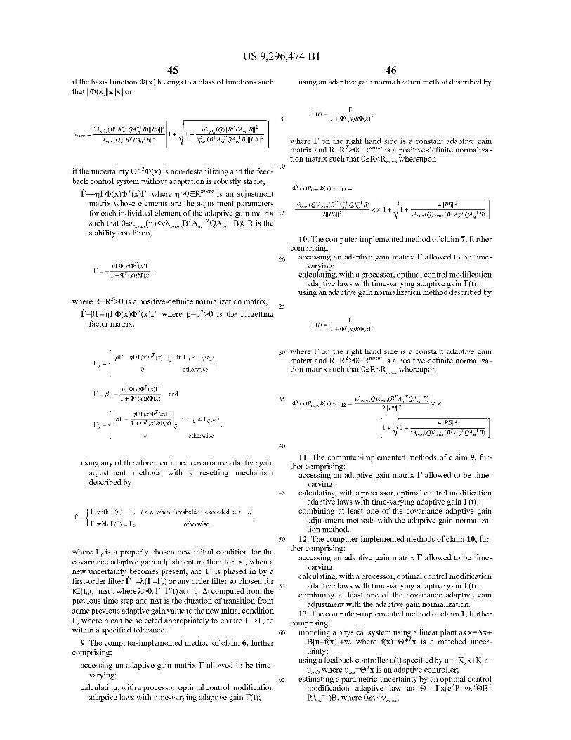
US 9,296,474 B1 45


46 using an adaptive gain normalization method described by

F 5 F(t) =

1 + (DT (x)R(D(x)

Um~ _ 2;L,s (BTAmTQAmiB)IIPBI12 1+ 1- gA ;n(Q)IIB T PAm'BIh

Ami,(Q)IIBTPAm'BIh Am2 ;n(BT AmT QAm1B)IIPBI1 2

if the uncertainty O* T(D(x) is non-destabilizing and the feed-back control system without adaptation is robustly stable,

I'=-gF(D(x)(D T(x)F, where q>OER-'- is an adjustment matrix whose elements are the adjustment parameters for each individual element of the adaptive gain matrix such that 0:5X_,,( ,q)<vX_i„(B TA_-TQAm-r B)ER is the stability condition,

gF(D(x)(DT (x)F

1 + (DT (x) R(D(x)'

where F on the right hand side is a constant adaptive gain matrix and R=RT>OER-'- is a positive-definite normaliza-tion matrix such that 0:5R<R m_ whereupon

10

(DT (x)Rm_(D(x) < C12 =

vAmi,(Q)Ami,(BT AmT QAmiB) x x 1 + 1 + 411PB112 15 211 pB11 2 vAmi, (Q)Ami, (BT AmT QA m- 1 B)


20 accessing an adaptive gain matrix F allowed to be time- varying;


using an adaptive gain normalization method described by where R=RT>O is a positive-definite normalization matrix, 25

I -PF-'gF(D(x)(D T(x)F, where P -P T>O is the forgetting factor matrix, F(t) _

1 + (DT (x)R(D(x)'

[/3C - qC(D(x)(DT (x)C] if C;~ <- Gij (to) C~~ _

0 otherwise

r/C(D(x)(DT (x)C' C

— F 1 +(DT(x)R(D(x)' and

gF(D(x)(DT (x)F

C.. = 1+(D (x)R(D(x)

0 otherwise

using any of the aforementioned covariance adaptive gain adjustment methods with a resetting mechanism described by

C with F(ti ) = [ ; t ? r, when threshold is exceeded at t = r, C-

C with C(0) = F O otherwise

where F, is a properly chosen new initial condition for the covariance adaptive gain adjustment method for t2A, when a new uncertainty becomes present, and F, is phased in by a first-order filter I=- ~ (I -I ~) or any order filter so chosen for tE[t ,t +nAt], where X>O, F-F(t) at t=t,-At computed from the previous time step and nAt is the duration of transition from some previous adaptive gain value to the new initial condition F, where n can be selected appropriately to ensure F—F, to within a specified tolerance.




30 where F on the right hand side is a constant adaptive gain matrix and R=RT>OER-x- is a positive-definite normaliza-tion matrix such that 0:5R<R m_ whereupon

35 (DT (x)Rm_ (D(x)ciz =

vAmi,(Q)Ami,(BTAmTQAm1B) x x

211PB11 2

411PBIF vAmi, (Q)A,~i. (BT AmT QAmi B)

40

11. The computer-implemented methods of claim 9, fur-ther comprising:


45 calculating, with a processor, optimal control modification adaptive laws with time-varying adaptive gain F(t);

combining at least one of the covariance adaptive gain adjustment methods with the adaptive gain normaliza-tion method.

50 12. The computer-implemented methods of claim 10, fur-ther comprising:


calculating, with a processor, optimal control modification 55 adaptive laws with time-varying adaptive gain F(t);

combining at least one of the covariance adaptive gain adjustment with the adaptive gain normalization.


60 modeling a physical system using a linear plant as x=Ax+ B[u+f(x)]+w, where f(x)=0* Tx is a matched uncer-tainty;

using a feedback controller u(t) specified by a=-K xx+K r- uad, where u_, O Tx is an adaptive controller; 65 estimating a parametric uncertainty by an optimal control

modification adaptive law as 0=-Fx(e TP-vxTOB T PA_- ')B, where 0:5v<vm_,

US 9,296,474 B1 47

using the linear asymptotic property whereupon 6-0 as t-- or whereupon L -t 0-0 under fast adaptation as L-- to establish the equilibrium value of the adaptive controller as uad O Tx-1/v(B TA_-TPB)-1 B TPe;

using the linear asymptotic property whereupon 6-0 as t-- or whereupon L -t 0-0 under fast adaptation as L-- to establish the linear feedback control system in the limit as X=(A m +1/vP-tA_ TP+BO* T)x-1/vP- 'A_T Pxm +Bmr+w, where the modification parameter v can be established such that the matrix A m +1/vP-tA_ TP+ BO* Tis a Hurwitz matrix to guarantee closed-loop sta-bility of the adaptive control system;

using the linear asymptotic property whereupon 6-0 as t-- or whereupon L -1 6-0 under fast adaptation as L-- to analyze the stability margins of the linear feed-back control system in the limit using linear time-invari-ant (LTI) methods to provide robustness of the adaptive control system;

using the linear asymptotic property whereupon 6-0 as t-- or whereupon L -1 6-0 under fast adaptation as F to compute the steady state tracking error in the limit as t-- or L—oo as limt--IFll_ —Am-1 Bm +(Am +I /vP-1 Am TP+BE) * T)-1 (I /vP—'Am T

PA_-t +I)B_Illlrll- which exhibits a linear input-output mapping to guarantee performance and provide predict-ability of the adaptive control system.


modeling a physical system using a input-delay linear plant as Xc Ax+B[u(t-t d)+f(x)]+, where f(x)=0* Tx is a matched uncertainty and t d is a given input time delay;

using the linear asymptotic property whereupon 6-0 as t-- or whereupon L -1 0-0 under fast adaptation as L-- to establish the linear feedback control system in the limit as X=(A+BO* T)x+(-BKxx+l/vP-Am TP)x(t-td)-1 /vP-tA_ TPxm (t-td)+B mr(t—td)+w, where the modi-fication parameter v can be established such that the matrix A_+1/vP-tA_ TP+BO* Tis a Hurwitz and the sta-bility condition detow-A,+Ade'" I-0 is satisfied or alternatively using the matrix measure method

td < 1 COS -

1 L

P(AI) +r(✓Ad)

W IlAdll J

where

A+BO*T 0 0

= u(-jAJ + IlAdll, A, = 0 Am 0 ana

1 0 0 —

td

BKx x— 1 P 1 AmP 1 P 1 Am P 0 V V

A d = 0 0 0

0 0 1 td

to guarantee closed-loop stability of the input-delay adaptive control system;

using the linear asymptotic property whereupon 6-0 as t-- or whereupon L -1 6-0 under fast adaptation as L-- to establish the linear feedback control system in the limit as X=(A+BO* T)x+(-BKxx+l/vP-Am TP)x(t-

48 td)-1/vP-tA_ TPxm(t-td)+Bmr(t-td)+w when r(t) is a constant command, where the modification parameter v can be established such that the matrix A m + 1/vP-IA_ TP+BO* Tis a Hurwitz and the stability condi-

5 tion detOw-A,+Ade'",I)-0 is satisfied or alternatively using the matrix measure method

10 t < lCOS i f u(AI)+u ( jAd) l d w L IlAdll J

where

15

=u(-jAJ+ IIAdl6 A + BO*T 0

A=- ~

0 Am

20

BKxx — ~ P-i A,T p ~ P-i AT~ P Ad = V V

25 0 0


30 using the linear asymptotic property whereupon 6-0 as t-- or whereupon L -1 6-0 under fast adaptation as L-- to establish the linear feedback control system in the limit as X=(A+BO* T)x+(-BKxx+l/vP-Am TP)x(t-td)+w when x_(t) and r(t) are constant or zero for an

35 adaptive regulator design, where the modification parameter v can be established such that the matrix Am +1/vP- 'A-TP+BO* T is a Hurwitz and the stability condition detUco-A-BO* T+

40 (BKxx-1/vP-tA_ TP)e'' tl-O is satisfied or alternatively using the matrix measure method where

1 F'A µ(A+BO* T)+ p(- j[BK—' ,T „P])

45 td <_ 1 COs 111111

BKx — ~ P-1 A,Tn P V

where w-u( jA jB0* r)+IIBKx 1/vP- 'A_TPII to guarantee 50 closed-loop stability of the input-delay adaptive control sys-

tem.

15. The computer-implemented method of claim 13, fur-ther comprising:

55 modeling a physical system using an input-delay linear plantas c Ax+B[u(t-td)+f(x)]+w, where f(x)=0* Txisa matched uncertainty and t d is a given input time delay;

using the linear asymptotic property whereupon 6-0 as 60 t-- or whereupon L-1 6-0 under fast adaptation as

L-- to establish the linear feedback control system in the limit as X=(A+BO* T)x+(-BKxx+l/vP-Am TP)x(t-td)-1/vP-tA_ TPxm(t-td)+Bmr(t-td)+w, where the modi-fication parameter v can be established such that the

65 matrix Am +l/vP-tA_ TP+BO* Tisa Hurwitz and the sta-bility condition detOw-A,+A de''td)-0 is satisfied or alternatively using the matrix measure method

US 9,296,474 B1 49

td < 1 COS 1L y(A, +y( ✓Ad)

IlAdll J

where

A+BO*T 0 0

= u(-jAJ +IlAdll, A, = 0 Am 0 , and 1

0 0 — td

BKxx - -P 'AmTP -P i AmP 0 V v

A d = 0 0 0

1 0 0 —

td


using the linear asymptotic property whereupon 6-0 as t-- or whereupon F - '0-0 under fast adaptation as F-- to establish the linear feedback control system in the limit as X=(A+BO* T)x+(-BKxx+l/vP-Am TP)x(t-td)-1/vP-rA_TPxm(t-td)+Bmr(t-td)+w when r(t) is a

constant command, where the modification parameter v can be established such that the matrix A m + 1/vP-r A_ TP+BO* T is a Hurwitz and the stability condi-tion det(jw-A,+Ade''td)-0 is satisfied or alternatively using the matrix measure method

td <- 1Cos i f µ(A,+µ(jAd ) l where W L IIAdII J

=u(- ✓AJ+IIAeIh A+BO*T 0

A~=~ 0 Am

and

A BKx x V 'Am p V 'A M P

d - 0 0


using the linear asymptotic property whereupon 6-0 as t-- or whereupon F - '0-0 under fast adaptation as F-- to establish the linear feedback control system in the limit as X=(A+BO* T)x+(-BKxx+l/vP-Am TP)x(t-td)+w when x_(t) and r(t) are constant or zero for an adaptive regulator design, where the modification parameter v can be established such that the matrix Am +1/vP-rA_ TP+BO* T is a Hurwitz and the stability condition det[jw-A-BO* T+(BKxx-1/vP-rA_ TP) e w -O is satisfied or alternatively using the matrix measure method

50

td <

1µ(A+BO*T)+ ~j[BK,-- V P-iA,TnP~~ COS

_1

,,, 111111 BKx - _ P -1 AT 5

where w-u( jA jB0* T)+IIBKx 1/vP-rA_ TPII to guarantee closed-loop stability of the input-delay adaptive control sys-

10 tem.


modeling a physical system using an input-delay linear 15 plant as c Ax+B[u(t--t d)+f(x)]+w, where f(x)=0* Tx is

a matched uncertainty and t d is a given input time delay;

using the linear asymptotic property whereupon 6-0 as t-- or whereupon F - '0-0 under fast adaptation as F-- to establish the linear feedback control system in

20 the limit as X=(A+BO* T)x+(-BKxx+l/vP-Am TP)x(t-td)-1/vP-rA_ TPxm (t-td)+Bmr(t-td)+w, where the modi-fication parameter v can be established such that the matrix A_+1/vP -rA_ TP+BO* Tis a Hurwitz and the sta-bility condition detOw-A e+Ade''tI-0 is satisfied or

25 alternatively using the matrix measure method

td < 1 COS - 1

L u(AI + f[(✓Ad)

W IlAdll J 30

where

35 A+BO* T 0 0

= u(-jAJ + IIAdII, A, - 0 Am 0 ,and 1

0 0 — td

40 BKxx- 1 P 1 AmP 1 P 1 AmP 0

V v

Ad - 0 0 0

0 0 1 td

45


using the linear asymptotic property whereupon 6-0 as So t-- or whereupon F- '0-0 under fast adaptation as

F-- to establish the linear feedback control system in the limit as X=(A+BO* T)x+(-BKxx+l/vP-rAm TP)x(t-t)-1/vP-rA_ TPxm(t-td)+B mr(t-td)+w when r(t) is a con-stant command, where the modification parameter v can

55 be established such that the matrix A m +1/vP-rA_ TP+ BO* T is a Hurwitz and the stability condition detow-AE+A,,&'tl-O is satisfied or alternatively using the matrix measure method

60

td <- lcos [p (A`)+µ(jAd ) l where

W L IIAdII J

1

A+BO* T 0

65 0 Am

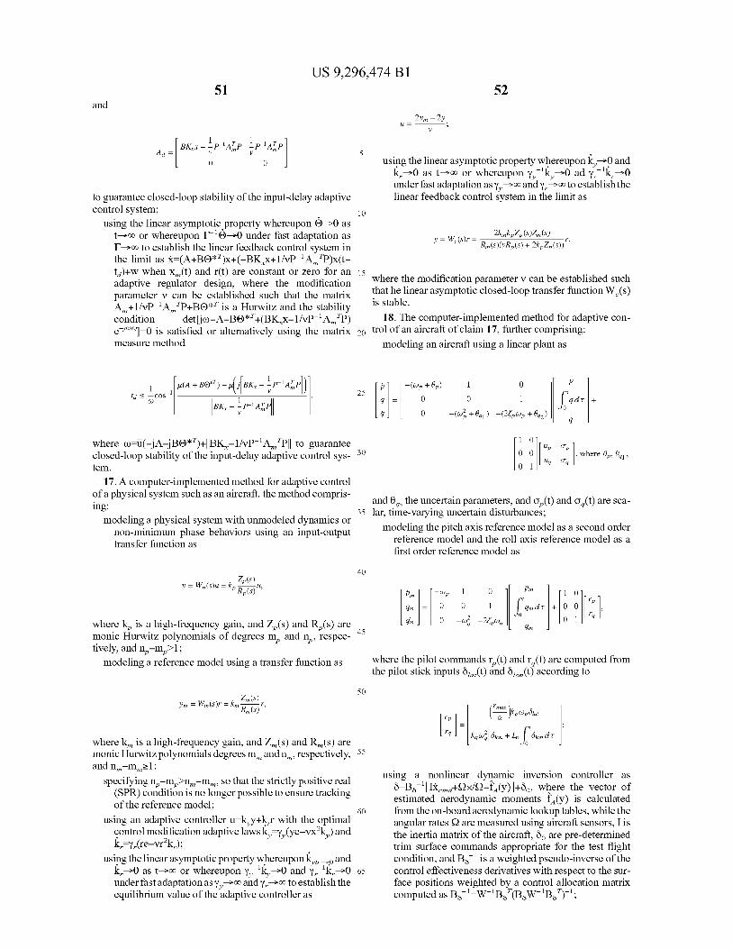
US 9,296,474 B1 51

52 and

ZYm - 2y u= ,

V

A d= BKx- yP'AmP V iAmP

e- 0 0


using the linear asymptotic property whereupon 6-0 as t-- or whereupon F - '0-0 under fast adaptation as F-- to establish the linear feedback control system in the limit as X=(A+BO* T)x+(-BKxx+l/vP-rAm TP)x(t-td)+w when x_(t) and r(t) are constant or zero for an adaptive regulator design, where the modification parameter v can be established such that the matrix Am +I/vP-rA_'P+BO* T is a Hurwitz and the stability condition detUco-A-BO* T+(BKxx-1/vP-rA_ TP) e'" I-0 is satisfied or alternatively using the matrix measure method

1 1 µ(A+BO,T)+

L ~~BKx - - V P

td

COS

_ 1

„ll<~

1 BK --P-1 A,Tn P

V

where w-u( jA jB0* T)+IIBKx I/vP-rA_ TPII to guarantee closed-loop stability of the input-delay adaptive control sys-tem.

17. A computer-implemented method for adaptive control of a physical system such as an aircraft, the method compris-ing:

modeling a physical system with unmodeled dynamics or non-minimum phase behaviors using an input -output transfer function as

Y = Wp (S)u = kp Rp(S)

u,

where kP is a high-frequency gain, and ZP (s) and RP(s) are monic Hurwitz polynomials of degrees mP and nP, respec-tively, and nP-mP>l;

modeling a reference model using a transfer function as

Z , (s) Ym = Wm (s)Y - km Wm—

(S) Y

where km is a high-frequency gain, and Z_(s) and R_(s) are monic Hurwitz polynomials degrees mm and nm, respectively, and nm-mm >-1;

specifying nP-mP>nm-mm, so that the strictly positive real (SPR) condition is no longer possible to ensure tracking of the reference model;

using an adaptive controller u=kyy+kx with the optimal control modification adaptive laws ky-yy(ye-vx'ky) and k,,_Y,.(re-vr2kr);

using the linear asymptotic property whereupon kyb —0 and k,.-0 as t-- or whereupon yy r ky,0 and yr r k,.,0 under fast adaptation as y y-- and y,.-- to establish the equilibrium value of the adaptive controller as

5 using the linear asymptotic property whereupon ky-0 and

k,.-0 as t-- or whereupon yy r ky-0 ad yr rk,.-0 under fast adaptation as y y-- and y,.-- to establish the linear feedback control system in the limit as

10

ZkmkpZp(s) m(s) Y= W~ (S)Y=

Rm (S)(vRp (s)+2kpZp(S))Y,

15 where the modification parameter v can be established such that he linear asymptotic closed-loop transfer function W,(s) is stable.

18. The computer-implemented method for adaptive con-20 trol of an aircraft of claim 17, further comprising:

modeling an aircraft using a linear plant as

p 1 0 P 25

g = 0 0 1 f}gdr ~ y 0

R 0 - (cop+ 9gi ) -(2Sp cop +Bgz )

1 0

30 0 0 up

- ~p ~ , where Bp , Bgi ,

0 1 U - Oq

and O qz the uncertain parameters , and 6P(t) and 6q(t) are sca-35 lar, time-varying uncertain disturbances;

modeling the pitch axis reference model as a second order reference model and the roll axis reference model as a first order reference model as

40

Pm -cop 1 0 1 Pm 1 0

l ff l

qm = 0 0 1 J gmdr +IO 0 Yp

J qm 0 _&)2 1

rq

45 q —ZS9~9 gm

where the pilot commands rp (t) and rq(t) are computed from the pilot stick inputs 6,, t(t) and 6 io„(t) according to

50

r (Yma

a ~kpcop6tar

Yq kg wg[6,+ 4 J Etondr] LL o 55

using a nonlinear dynamic inversion controller as 6=B8- r [IX,md+Qx/Q-f,(y)J +6o, where the vector of estimated aerodynamic moments f, (y) is calculated

60 from the on-board aerodynamic lookup tables, while the angular rates Q are measured using aircraft sensors, I is the inertia matrix of the aircraft, 6 0 are pre-determined trim surface commands appropriate for the test flight condition , and B,- ' is a weighted pseudo -inverse of the

65 control effectiveness derivatives with respect to the sur-face positions weighted by a control allocation matrix computed as Bb r=W-r BbT(B,5W-r B,5 )-r;

US 9,296,474 B1 53

modeling the angular acceleration commands and

P,f + P, + Pa

x—d W=z,f+ z, + k, = g,f+g,+ga

prf+ p 5

as the sum of the desired reference dynamics X,, f(t) produced by the nonlinear dynamic inversion reference model, the out-put X,(t) of the error compensator, and adaptive control aug-mentation X a(t); 10

using the nonlinear dynamic inversion adaptive flight controller to cancel out the effects of the uncertain parameters 6P, 6 q,, 0,,, ,,(t), and aq(t) by the adaptive augmentation controller

15

uv ry + Pa Pa BPp+ & P

— ,where — ( ~̀

uq rP + 4a 4, 9qi J g d r + 9q, g + &g 0

estimating the uncertain parameters by the optimal control 20 modification adaptive laws with adaptive gain normal-ization as

BP =

F, 25 z IPPPPBm❑ + voP p'B,Bm P PP A m' BmP)

25 1+NoP p

rejecting disturbances by the optimal control modification adaptive laws with adaptive gain normalization plus dis-turbance rejection as

0, 1+Nc P2(PPPBmP+vc,B,BmPPPAMPBmP) P

and

9 = F,a (zT P B,,,q + V Cq & Bm q P Amg B mq ). 9 1 +xq NQq xP q 9 9 9

54

9q = Toa (xgzgPg B q +vog xg xg9q Bm q Pq Amq Mq ), where 1 + xq Noq xP

9q = 9qi 9q2 ]T, P = Pm — P,

T r T

xq = f qdT g aI1Cj XP = L f (qm - g)dT Qm - Q J 0 0

us000009296474b120160329 - nasa · us 9,296,474 b1 page 2 (56) references cited other publications...

Documents