General rights Copyright and moral rights for the publications made accessible in the public portal are retained by the authors and/or other copyright owners and it is a condition of accessing publications that users recognise and abide by the legal requirements associated with these rights.

Users may download and print one copy of any publication from the public portal for the purpose of private study or research.

You may not further distribute the material or use it for any profit-making activity or commercial gain

You may freely distribute the URL identifying the publication in the public portal If you believe that this document breaches copyright please contact us providing details, and we will remove access to the work immediately and investigate your claim.

Downloaded from orbit.dtu.dk on: Oct 23, 2021

UR10 Performance Analysis

Ravn, Ole; Andersen, Nils Axel; Andersen, Thomas Timm

Publication date:2014

Document VersionPublisher's PDF, also known as Version of record

Link back to DTU Orbit

Citation (APA):Ravn, O., Andersen, N. A., & Andersen, T. T. (2014). UR10 Performance Analysis. Technical University ofDenmark, Department of Electrical Engineering.

UR10 Performance Analysis

by Asger Winther-Jørgensen& Christian Ahlburg Dirksen

Technical University of DenmarkInstitute for Automation and ControlOle RavnNils Axel AndersenThomas Timm Andersen29. juni 2014

Contents

Contents i

1 Introduction 1

2 Real-time Interface 22.1 Congestion Control - Nagle’s algorithm? . . . . . . . . . . . . . 22.2 Sample Frequency . . . . . . . . . . . . . . . . . . . . . . . . . 52.3 Calculation time and delays . . . . . . . . . . . . . . . . . . . . 8

3 Commands 113.1 The movec command . . . . . . . . . . . . . . . . . . . . . . . . 133.2 The movej command . . . . . . . . . . . . . . . . . . . . . . . . 143.3 The movel command . . . . . . . . . . . . . . . . . . . . . . . . 163.4 The servoj and servoc commands . . . . . . . . . . . . . . . . . 173.5 The speedj command . . . . . . . . . . . . . . . . . . . . . . . . 173.6 The speedl command . . . . . . . . . . . . . . . . . . . . . . . . 173.7 The stopj command . . . . . . . . . . . . . . . . . . . . . . . . 243.8 The stopl command . . . . . . . . . . . . . . . . . . . . . . . . 25

4 Conclusion 28

i

1 Introduction

While working with the UR-10 robot arm, it has become apparent that somecommands have undesired behaviour when operating the robot arm through asocket connection, sending one command at a time. This report is a collectionof the results optained when testing the performance of the different commandsavailable in URScript to control the robot. It will also describe the differenttime delays discovered when using the UR-10 robot arm.

1

2 Real-time Interface

Glossary for the following sections:Controller:The program running on the UR-10’s internal computer, broadcasting robotarm data, recieving and interpretting commands and controlling the armaccordingly.Interfacing program or program:A program running on an arbitrary computer, connecting (interfacing) with thecontroller over a TCP Connection to the controller’s ’real time’- or MATLAB-Interface port.

2.1 Congestion Control - Nagle’s algorithm?The first thing that becomes evident when looking at the Matlab interfaceoutput of the UR-10 robot is that it appears to have some sort of anti-congestionalgorithm in place.

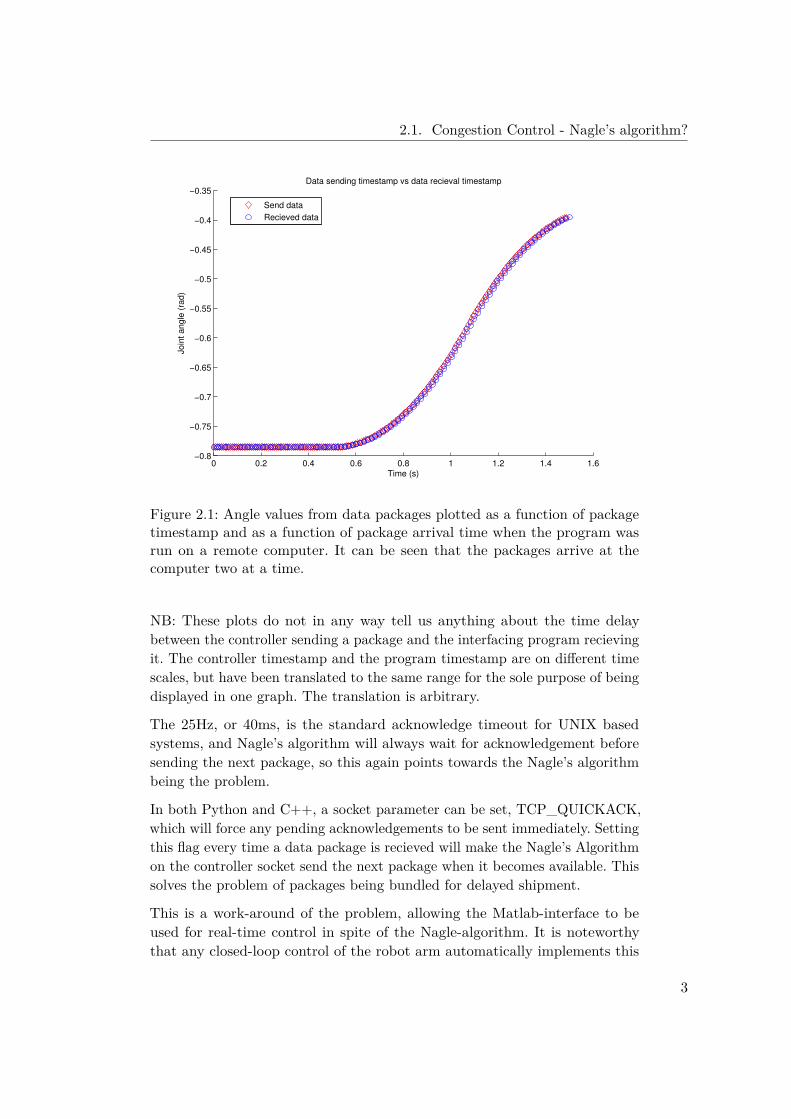
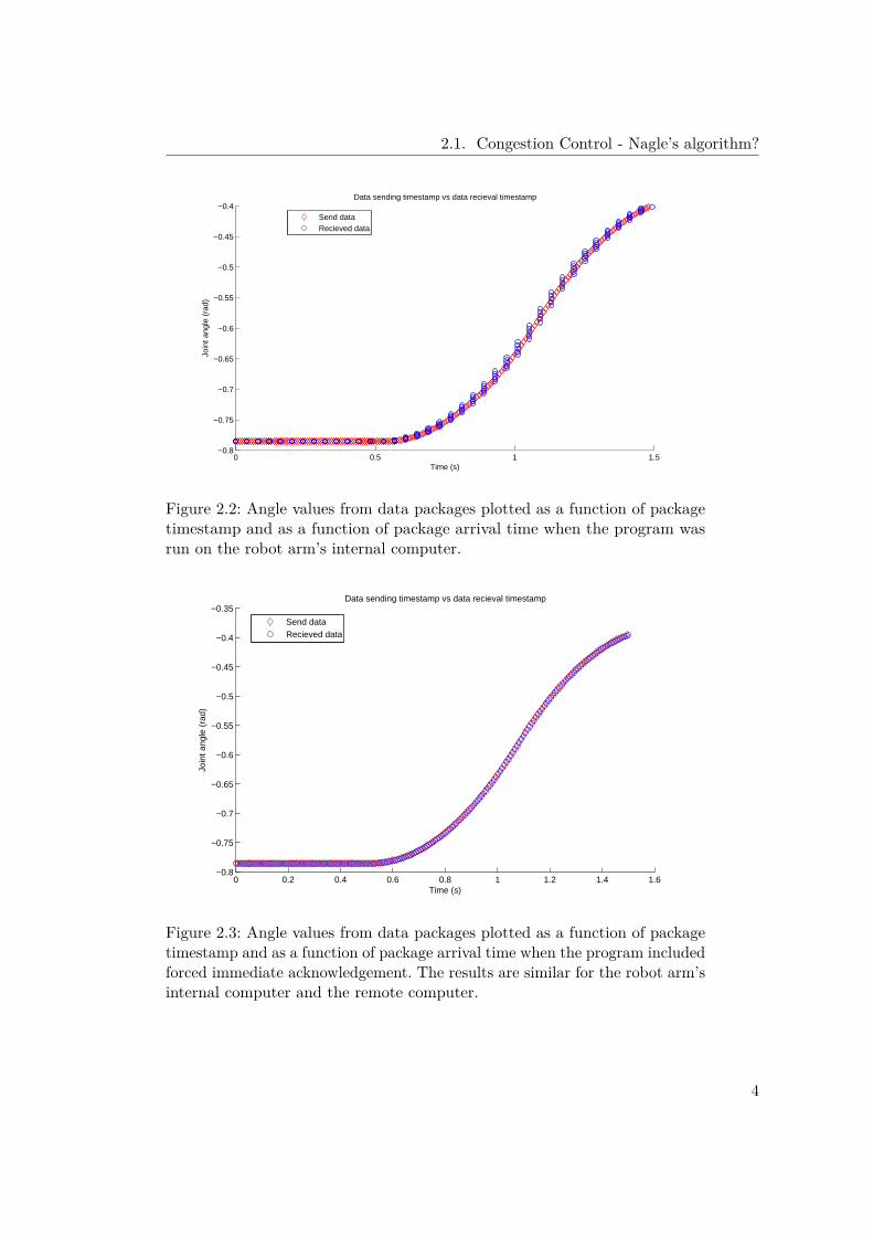
Figures 2.1 and 2.2 show a joint angle as a function of time. In each of thefigures, the two series are the same joint-variables plotted as functions of twodifferent times. The red series is the joint angle as a function of the timestampof the package in which it was broadcast. The blue series is the very same jointangle data series, but this time plotted as a function of the computer localtimeat which the package was recieved by the program communicating with theUR Matlab interface.

In figure 2.1 the program was run on a remote computer communicating withthe robot arm’s internal computer over Ethernet. In figure 2.2 the programwas run on the robot arm’s internal computer.

Especially in figure 2.2, it is very visible that the packages are not broadcastat a rate of 125Hz, but rather at some other frequency, in this case 5 packagesat a time at 25Hz, approximately. For this test, the program interfacing withthe Matlab interface was run on the robot arm’s internal computer.

2

2.1. Congestion Control - Nagle’s algorithm?

0 0.2 0.4 0.6 0.8 1 1.2 1.4 1.6−0.8

−0.75

−0.7

−0.65

−0.6

−0.55

−0.5

−0.45

−0.4

−0.35Data sending timestamp vs data recieval timestamp

Time (s)

Join

t angle

(ra

d)

Send data

Recieved data

Figure 2.1: Angle values from data packages plotted as a function of packagetimestamp and as a function of package arrival time when the program wasrun on a remote computer. It can be seen that the packages arrive at thecomputer two at a time.

NB: These plots do not in any way tell us anything about the time delaybetween the controller sending a package and the interfacing program recievingit. The controller timestamp and the program timestamp are on different timescales, but have been translated to the same range for the sole purpose of beingdisplayed in one graph. The translation is arbitrary.

The 25Hz, or 40ms, is the standard acknowledge timeout for UNIX basedsystems, and Nagle’s algorithm will always wait for acknowledgement beforesending the next package, so this again points towards the Nagle’s algorithmbeing the problem.

In both Python and C++, a socket parameter can be set, TCP_QUICKACK,which will force any pending acknowledgements to be sent immediately. Settingthis flag every time a data package is recieved will make the Nagle’s Algorithmon the controller socket send the next package when it becomes available. Thissolves the problem of packages being bundled for delayed shipment.

This is a work-around of the problem, allowing the Matlab-interface to beused for real-time control in spite of the Nagle-algorithm. It is noteworthythat any closed-loop control of the robot arm automatically implements this

3

2.1. Congestion Control - Nagle’s algorithm?

0 0.5 1 1.5−0.8

−0.75

−0.7

−0.65

−0.6

−0.55

−0.5

−0.45

−0.4Data sending timestamp vs data recieval timestamp

Time (s)

Join

t ang

le (

rad)

Send dataRecieved data

Figure 2.2: Angle values from data packages plotted as a function of packagetimestamp and as a function of package arrival time when the program wasrun on the robot arm’s internal computer.

0 0.2 0.4 0.6 0.8 1 1.2 1.4 1.6−0.8

−0.75

−0.7

−0.65

−0.6

−0.55

−0.5

−0.45

−0.4

−0.35Data sending timestamp vs data recieval timestamp

Time (s)

Join

t ang

le (

rad)

Send dataRecieved data

Figure 2.3: Angle values from data packages plotted as a function of packagetimestamp and as a function of package arrival time when the program includedforced immediate acknowledgement. The results are similar for the robot arm’sinternal computer and the remote computer.

4

2.2. Sample Frequency

work-around since sending a command as a reaction to the last recieved packagewill also send the acknowledgement so that the next package will appear ontime.

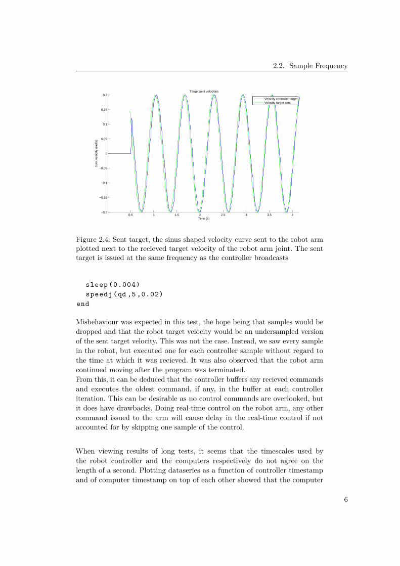
2.2 Sample FrequencyNow that the recieving frequency has been determined to be 125Hz, it wouldbe good to know the frequency with which one can send commands to therobot arm and expect them to be handled on time. To see if this frequencymatched the broadcasting frequency, a sampled sinus curve was sent to therobot arm, one sample pr. recieved data package from the robot arm. Figure2.4 displays the result of a test in which a sinusoidal velocity curve for one jointwas sent to the robot arm at the same frequency the robot arm broadcastswith, achieved by sending each sample as a reaction to a recieved package.Here the code used was:

starttime = time.nowwhile time.now < 2*pi+ starttime :

on recieved_new_data :qd = [0 ,0 ,0 ,0 ,0 ,0]qd [4] = sin (10* time.now)speedj (qd ,5 ,0.02)

end

What can be seen on the figure is that the robot arm’s internal target velocityfollows, with some delay, the same trajectory as is sent to it, that is it doesnot undersample or drop packages.Something else to notice is the sometimes serrated nature of the controllertarget velocity curve. It seems that commands are lost one sample, but madeup for in the next. This suggests that the controller handles input and outputasynchronously. This serration also shows that, even though these commandsare sent as soon as possible after recieving a package, one cannot be sure thata reaction will be seen until two samples later.

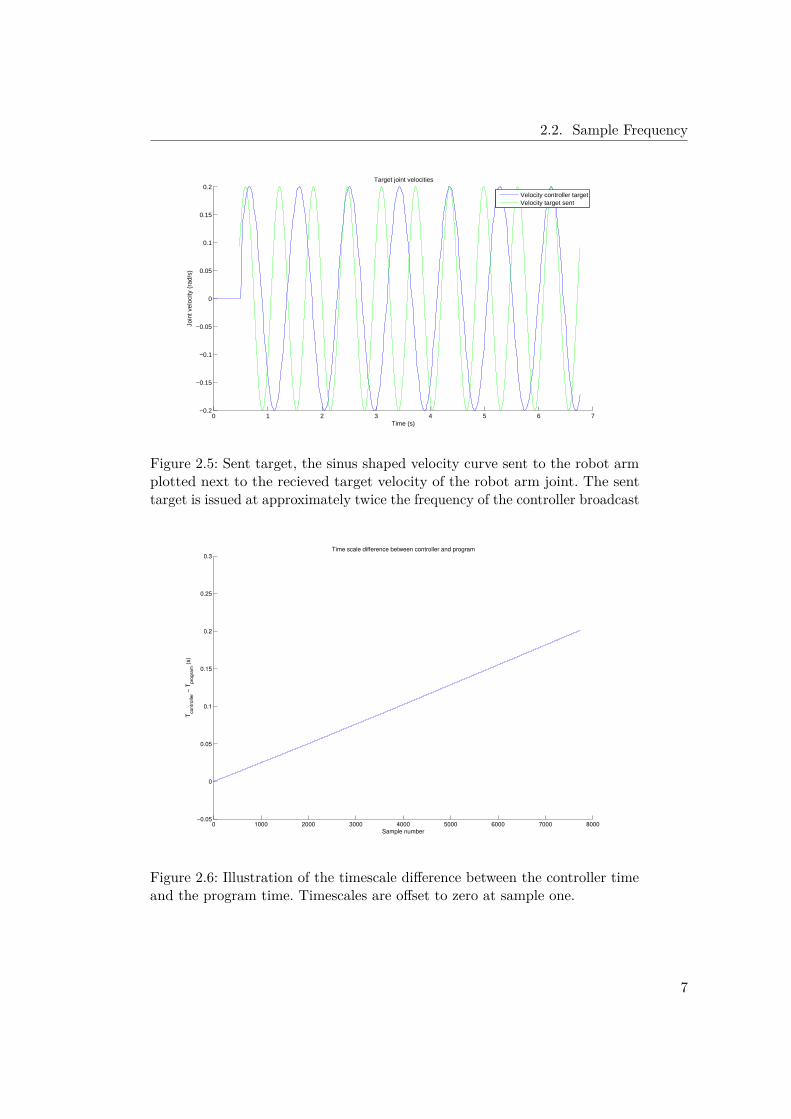
Looking at figure 2.5 we see a different behaviour. In this case, the samesinusoidal curve was sent to the robot arm, but at twice the frequency, that isboth the frequenuncy of the sinusoidal curve and the sample frequency weredoubled. The code used here was:

starttime = time.nowwhile time.now < 2*pi+ starttime :

qd = [0 ,0 ,0 ,0 ,0 ,0]qd [4] = sin (11* time.now)

5

2.2. Sample Frequency

0.5 1 1.5 2 2.5 3 3.5 4−0.2

−0.15

−0.1

−0.05

0

0.05

0.1

0.15

0.2Target joint velocities

Time (s)

Join

t vel

ocity

(ra

d/s)

Velocity controller targetVelocity target sent

Figure 2.4: Sent target, the sinus shaped velocity curve sent to the robot armplotted next to the recieved target velocity of the robot arm joint. The senttarget is issued at the same frequency as the controller broadcasts

sleep (0.004)speedj (qd ,5 ,0.02)

end

Misbehaviour was expected in this test, the hope being that samples would bedropped and that the robot target velocity would be an undersampled versionof the sent target velocity. This was not the case. Instead, we saw every samplein the robot, but executed one for each controller sample without regard tothe time at which it was recieved. It was also observed that the robot armcontinued moving after the program was terminated.From this, it can be deduced that the controller buffers any recieved commandsand executes the oldest command, if any, in the buffer at each controlleriteration. This can be desirable as no control commands are overlooked, butit does have drawbacks. Doing real-time control on the robot arm, any othercommand issued to the arm will cause delay in the real-time control if notaccounted for by skipping one sample of the control.

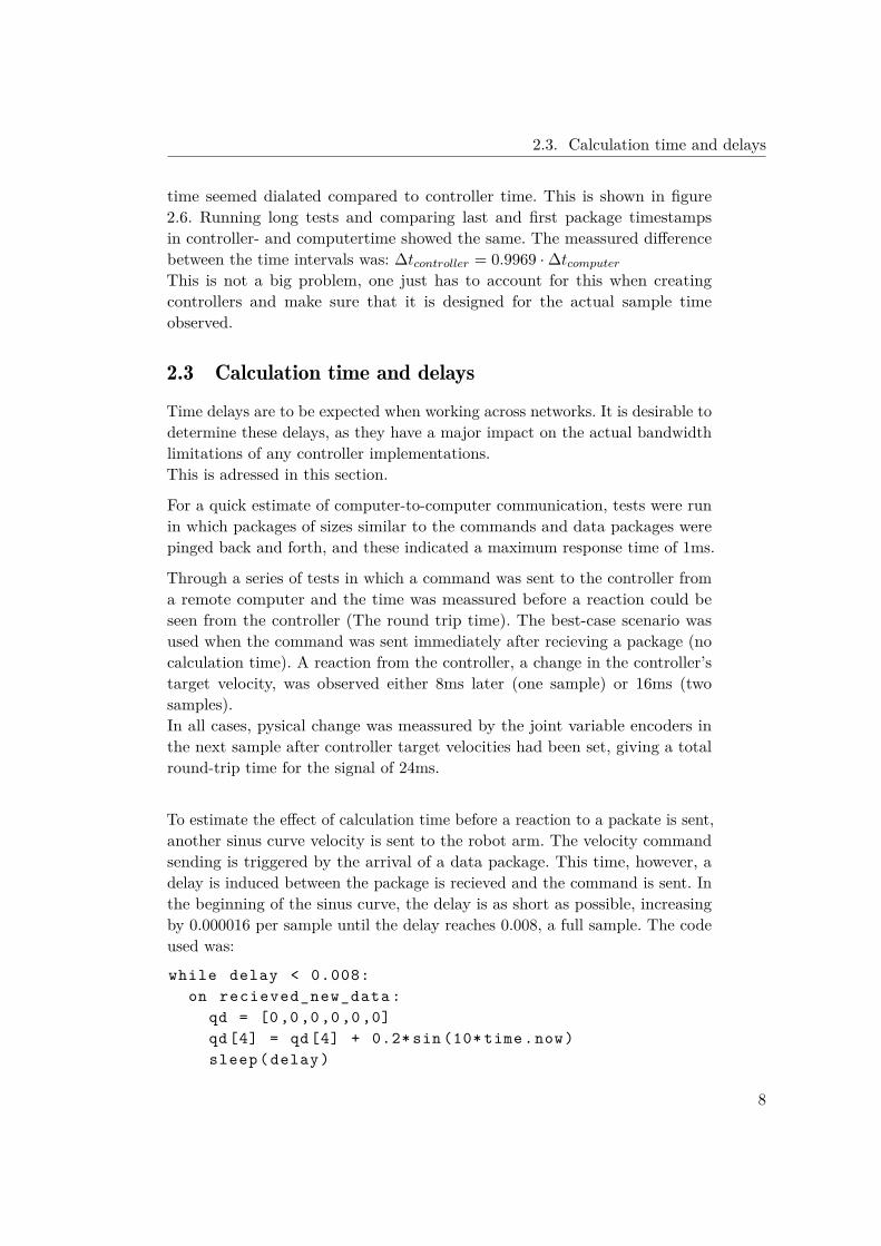
When viewing results of long tests, it seems that the timescales used bythe robot controller and the computers respectively do not agree on thelength of a second. Plotting dataseries as a function of controller timestampand of computer timestamp on top of each other showed that the computer

6

2.2. Sample Frequency

0 1 2 3 4 5 6 7−0.2

−0.15

−0.1

−0.05

0

0.05

0.1

0.15

0.2Target joint velocities

Time (s)

Join

t vel

ocity

(ra

d/s)

Velocity controller targetVelocity target sent

Figure 2.5: Sent target, the sinus shaped velocity curve sent to the robot armplotted next to the recieved target velocity of the robot arm joint. The senttarget is issued at approximately twice the frequency of the controller broadcast

0 1000 2000 3000 4000 5000 6000 7000 8000−0.05

0

0.05

0.1

0.15

0.2

0.25

0.3Time scale difference between controller and program

Sample number

Tcontr

olle

r − T

pro

gra

m (

s)

Figure 2.6: Illustration of the timescale difference between the controller timeand the program time. Timescales are offset to zero at sample one.

7

2.3. Calculation time and delays

time seemed dialated compared to controller time. This is shown in figure2.6. Running long tests and comparing last and first package timestampsin controller- and computertime showed the same. The meassured differencebetween the time intervals was: ∆tcontroller = 0.9969 · ∆tcomputer

This is not a big problem, one just has to account for this when creatingcontrollers and make sure that it is designed for the actual sample timeobserved.

2.3 Calculation time and delaysTime delays are to be expected when working across networks. It is desirable todetermine these delays, as they have a major impact on the actual bandwidthlimitations of any controller implementations.This is adressed in this section.

For a quick estimate of computer-to-computer communication, tests were runin which packages of sizes similar to the commands and data packages werepinged back and forth, and these indicated a maximum response time of 1ms.

Through a series of tests in which a command was sent to the controller froma remote computer and the time was meassured before a reaction could beseen from the controller (The round trip time). The best-case scenario wasused when the command was sent immediately after recieving a package (nocalculation time). A reaction from the controller, a change in the controller’starget velocity, was observed either 8ms later (one sample) or 16ms (twosamples).In all cases, pysical change was meassured by the joint variable encoders inthe next sample after controller target velocities had been set, giving a totalround-trip time for the signal of 24ms.

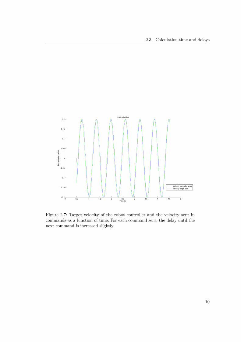
To estimate the effect of calculation time before a reaction to a packate is sent,another sinus curve velocity is sent to the robot arm. The velocity commandsending is triggered by the arrival of a data package. This time, however, adelay is induced between the package is recieved and the command is sent. Inthe beginning of the sinus curve, the delay is as short as possible, increasingby 0.000016 per sample until the delay reaches 0.008, a full sample. The codeused was:

while delay < 0.008:on recieved_new_data :

qd = [0 ,0 ,0 ,0 ,0 ,0]qd [4] = qd [4] + 0.2* sin (10* time.now)sleep(delay)

8

2.3. Calculation time and delays

delay += 0.008/500speedj (qd ,5 ,0.02)

sleep (0.00001)end

One resulting graph is shown in 2.7. It can be seen that the target velocitygraph is serrated in the beginning of the graph, indicating that the commandsdo not consistently take the same amount of samples before reaching thecontroller, as was seen when meassuring reaction times for immediate respon-ses. This serration is caused mainly by network and calculation time, and itis suspected that the controller interacts with network data and the robotasynchronious. Upon reaching a certain delay, the commands consistently reachthe target velocity of the controller in two samples. Serration shows again at a6ms delay, indicating that at a calculation time of less than 6ms will ensurethat a command reaches the controller in maximum 2 samples (16ms), andthat physical change can be seen within 3 samples (24ms).

This gives a total of somewhere between 16ms and 24ms from a command isissued until a physical change can be observed in the system. This results in abandwidth limit of approximately 50Hz induced by the delays in communica-tion in the best-case scenario where calculation time is less than 6ms and therobot arm and controlling computer are on the same local wired network.

These results are valid for programs run on a remote computer connected overethernet and for the robot arm’s internal computer alike.

9

2.3. Calculation time and delays

0 0.5 1 1.5 2 2.5 3 3.5 4 4.5 5−0.2

−0.15

−0.1

−0.05

0

0.05

0.1

0.15

0.2Joint velocities

Time (s)

Join

t velo

city (

rad/s

)

Velocity controller target

Velocity target sent

Figure 2.7: Target velocity of the robot controller and the velocity sent incommands as a function of time. For each command sent, the delay until thenext command is increased slightly.

10

3 Commands

The UR script provides a series of commands with which to control the robotarm. Each have their uses and caveats. Some tests of a selection of thesecommands have been run, and some of these problems have been documented.Table 3.1 shows a list of the tested commands, short descriptions of them anda brief summary of the test results in good/bad form. Extended explanationsof the tests and results follow where they have been deemed worthwhile.

11

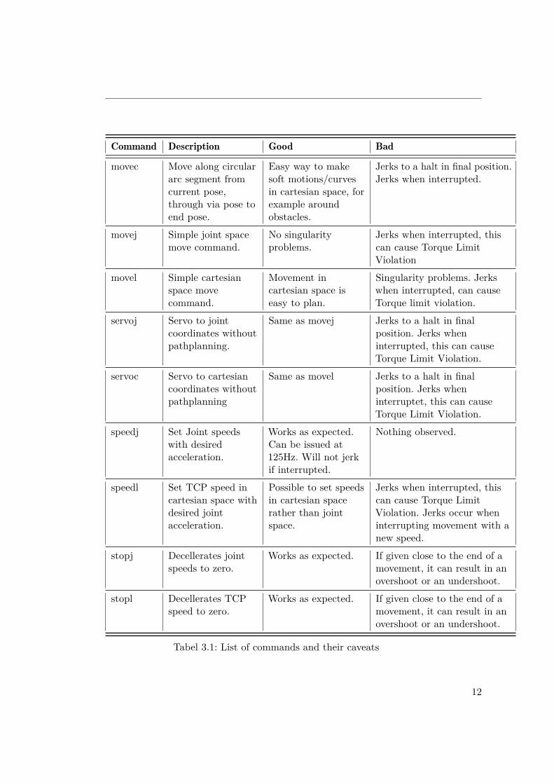
Command Description Good Bad

movec Move along circulararc segment fromcurrent pose,through via pose toend pose.

Easy way to makesoft motions/curvesin cartesian space, forexample aroundobstacles.

Jerks to a halt in final position.Jerks when interrupted.

movej Simple joint spacemove command.

No singularityproblems.

Jerks when interrupted, thiscan cause Torque LimitViolation

movel Simple cartesianspace movecommand.

Movement incartesian space iseasy to plan.

Singularity problems. Jerkswhen interrupted, can causeTorque limit violation.

servoj Servo to jointcoordinates withoutpathplanning.

Same as movej Jerks to a halt in finalposition. Jerks wheninterrupted, this can causeTorque Limit Violation.

servoc Servo to cartesiancoordinates withoutpathplanning

Same as movel Jerks to a halt in finalposition. Jerks wheninterruptet, this can causeTorque Limit Violation.

speedj Set Joint speedswith desiredacceleration.

Works as expected.Can be issued at125Hz. Will not jerkif interrupted.

Nothing observed.

speedl Set TCP speed incartesian space withdesired jointacceleration.

Possible to set speedsin cartesian spacerather than jointspace.

Jerks when interrupted, thiscan cause Torque LimitViolation. Jerks occur wheninterrupting movement with anew speed.

stopj Decellerates jointspeeds to zero.

Works as expected. If given close to the end of amovement, it can result in anovershoot or an undershoot.

stopl Decellerates TCPspeed to zero.

Works as expected. If given close to the end of amovement, it can result in anovershoot or an undershoot.

Tabel 3.1: List of commands and their caveats

12

3.1. The movec command

3.1 The movec commandThe code for this test:

sleep (0.5)movec(pvia,pend ,2 ,0.6)sleep (5)

0 1 2 3 4 5 6−0.3

−0.2

−0.1

0

0.1

0.2

0.3

0.4

0.5Target Joint velocities

Time (s)

Join

t velo

city (

rad/s

)

Joint 1

Joint 2

Joint 3

Joint 4

Joint 5

Joint 6

Figure 3.1: Target joint velocities during a movec command execution.

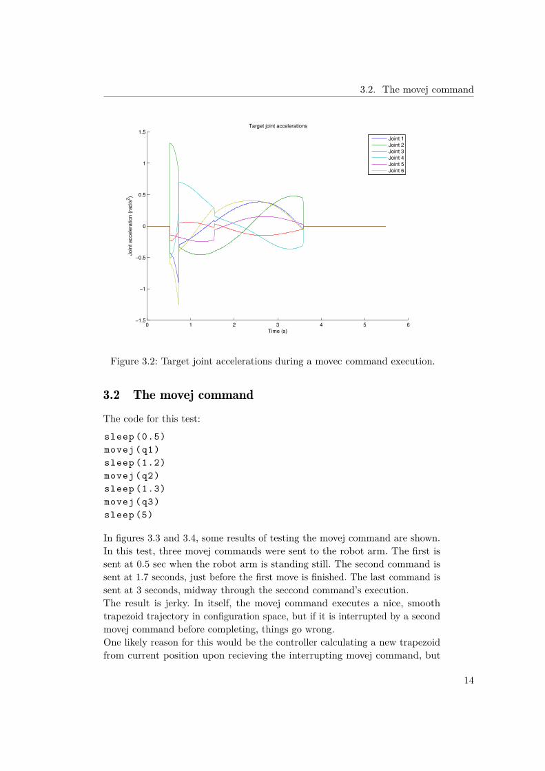
In figures 3.1 and 3.2 the behaviour of movec can be seen.When the movec reaches it’s final pose, the robot arm jerks violently to a halt,inducing notable vibrations in the robot setup. Looking at the target velocitycurve, one could expect the target accelerations to be off the charts, similarto when move commands in general are interrupted, but this does not occuraccording to figure 3.2. It seems that the controller just abandons the robot toit’s own devices once the goal position is reached.The lack of deceleration is an issue, but the lack of effort to break instantlydoes save the system from joint torque limit violation.

13

3.2. The movej command

0 1 2 3 4 5 6−1.5

−1

−0.5

0

0.5

1

1.5Target joint accelerations

Time (s)

Join

t accele

ration (

rad/s

2)

Joint 1

Joint 2

Joint 3

Joint 4

Joint 5

Joint 6

Figure 3.2: Target joint accelerations during a movec command execution.

3.2 The movej commandThe code for this test:

sleep (0.5)movej(q1)sleep (1.2)movej(q2)sleep (1.3)movej(q3)sleep (5)

In figures 3.3 and 3.4, some results of testing the movej command are shown.In this test, three movej commands were sent to the robot arm. The first issent at 0.5 sec when the robot arm is standing still. The second command issent at 1.7 seconds, just before the first move is finished. The last command issent at 3 seconds, midway through the seccond command’s execution.The result is jerky. In itself, the movej command executes a nice, smoothtrapezoid trajectory in configuration space, but if it is interrupted by a secondmovej command before completing, things go wrong.One likely reason for this would be the controller calculating a new trapezoidfrom current position upon recieving the interrupting movej command, but

14

3.2. The movej command

0 1 2 3 4 5 6 7 8−60

−40

−20

0

20

40

60Target joint accelerations

Time (s)

Join

t accele

ration (

rad/s

2)

Joint 1

Joint 2

Joint 3

Joint 4

Joint 5

Joint 6

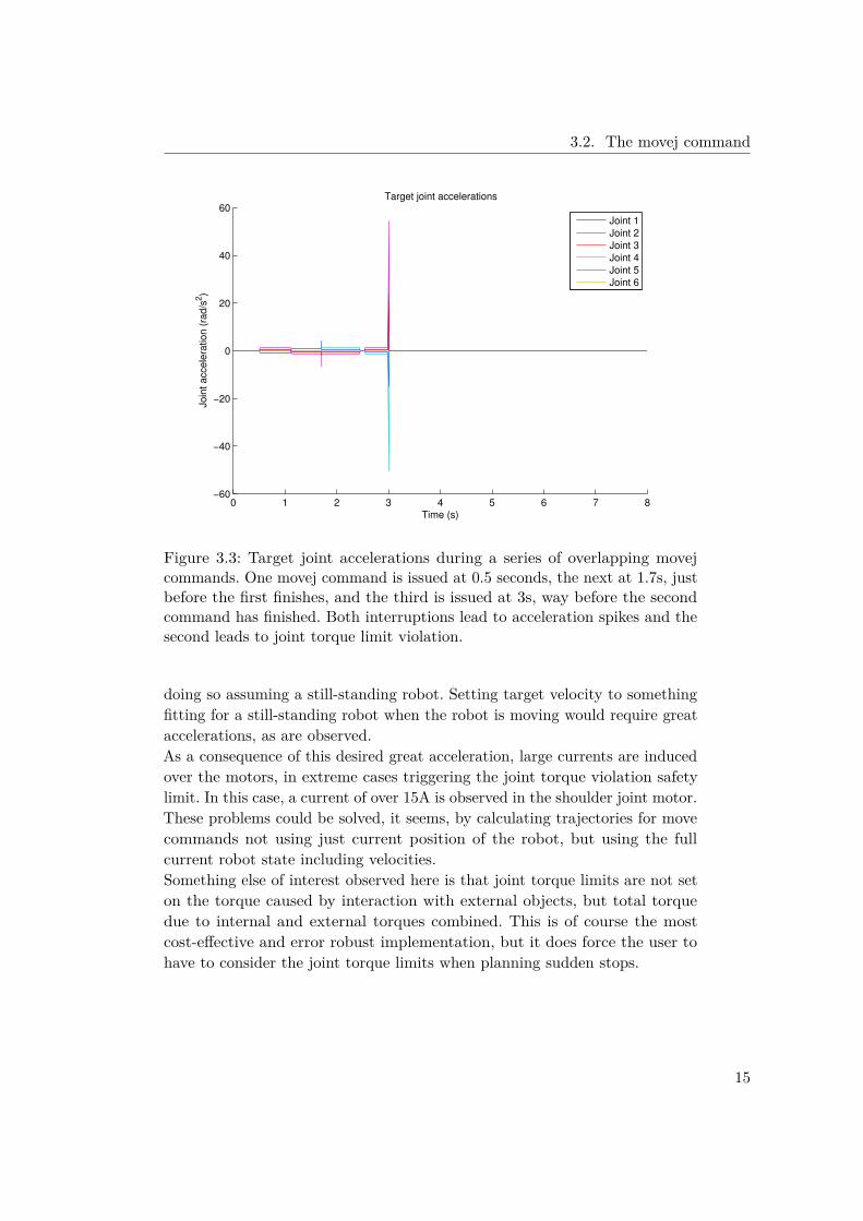
Figure 3.3: Target joint accelerations during a series of overlapping movejcommands. One movej command is issued at 0.5 seconds, the next at 1.7s, justbefore the first finishes, and the third is issued at 3s, way before the secondcommand has finished. Both interruptions lead to acceleration spikes and thesecond leads to joint torque limit violation.

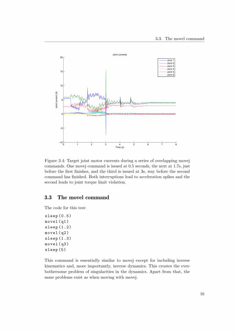
doing so assuming a still-standing robot. Setting target velocity to somethingfitting for a still-standing robot when the robot is moving would require greataccelerations, as are observed.As a consequence of this desired great acceleration, large currents are inducedover the motors, in extreme cases triggering the joint torque violation safetylimit. In this case, a current of over 15A is observed in the shoulder joint motor.These problems could be solved, it seems, by calculating trajectories for movecommands not using just current position of the robot, but using the fullcurrent robot state including velocities.Something else of interest observed here is that joint torque limits are not seton the torque caused by interaction with external objects, but total torquedue to internal and external torques combined. This is of course the mostcost-effective and error robust implementation, but it does force the user tohave to consider the joint torque limits when planning sudden stops.

15

3.3. The movel command

0 1 2 3 4 5 6 7 8−10

−5

0

5

10

15

20Joint currents

Time (s)

Jo

int

curr

ent (A

)

Joint 1

Joint 2

Joint 3

Joint 4

Joint 5

Joint 6

Figure 3.4: Target joint motor currents during a series of overlapping movejcommands. One movej command is issued at 0.5 seconds, the next at 1.7s, justbefore the first finishes, and the third is issued at 3s, way before the secondcommand has finished. Both interruptions lead to acceleration spikes and thesecond leads to joint torque limit violation.

3.3 The movel commandThe code for this test:

sleep (0.5)movel(q1)sleep (1.2)movel(q2)sleep (1.3)movel(q3)sleep (5)

This command is essentially similar to movej except for including inversekinematics and, more importantly, inverse dynamics. This creates the ever-bothersome problem of singularities in the dynamics. Apart from that, thesame problems exist as when moving with movej.

16

3.4. The servoj and servoc commands

3.4 The servoj and servoc commandsThe code for this test:

sleep (0.5)servoj (q ,0 ,0 ,0.8)sleep (1)

These command seems to be essentially a less useful version of movej and movel.They do the job of getting from A to B, but the same stopping behaviour aswith movec is exhibited, making the use of this command slightly faster andmassively more jerky.

3.5 The speedj commandThis command seems to be the only command useful for control real-timecontrol of the robot.The robot accelerates to a set of joint velocities, both velocities and accelerationsprovided by the user. No combination of interruptions was found that wouldmake the robot attempt accelerations exeeding what was sent in the command.

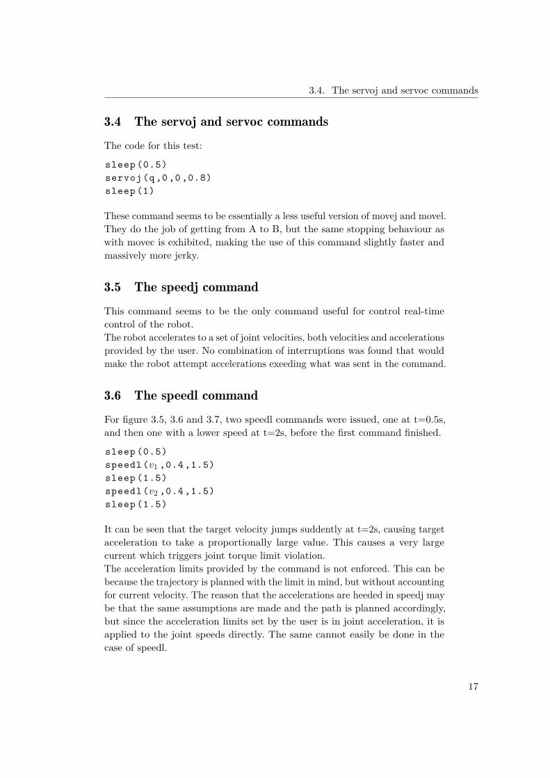
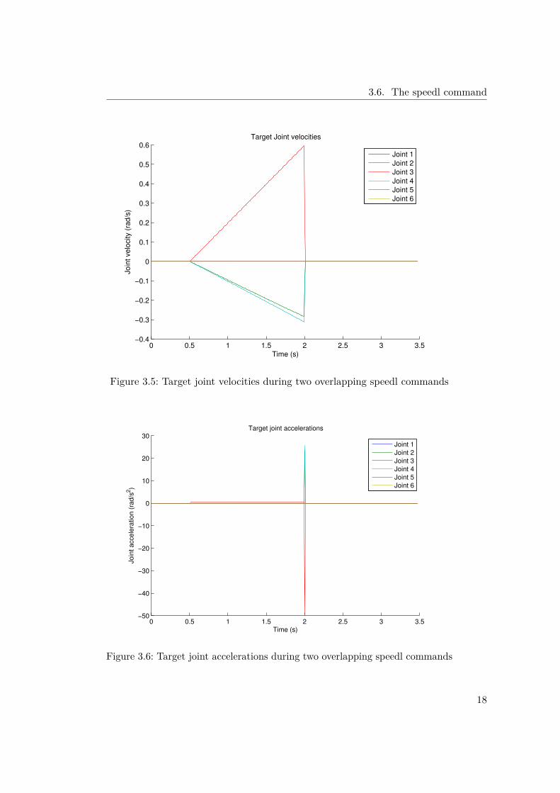
3.6 The speedl commandFor figure 3.5, 3.6 and 3.7, two speedl commands were issued, one at t=0.5s,and then one with a lower speed at t=2s, before the first command finished.

sleep (0.5)speedl (v1 ,0.4 ,1.5)sleep (1.5)speedl (v2 ,0.4 ,1.5)sleep (1.5)

It can be seen that the target velocity jumps suddently at t=2s, causing targetacceleration to take a proportionally large value. This causes a very largecurrent which triggers joint torque limit violation.The acceleration limits provided by the command is not enforced. This can bebecause the trajectory is planned with the limit in mind, but without accountingfor current velocity. The reason that the accelerations are heeded in speedj maybe that the same assumptions are made and the path is planned accordingly,but since the acceleration limits set by the user is in joint acceleration, it isapplied to the joint speeds directly. The same cannot easily be done in thecase of speedl.

17

3.6. The speedl command

0 0.5 1 1.5 2 2.5 3 3.5−0.4

−0.3

−0.2

−0.1

0

0.1

0.2

0.3

0.4

0.5

0.6Target Joint velocities

Time (s)

Jo

int

ve

locity (

rad

/s)

Joint 1

Joint 2

Joint 3

Joint 4

Joint 5

Joint 6

Figure 3.5: Target joint velocities during two overlapping speedl commands

0 0.5 1 1.5 2 2.5 3 3.5−50

−40

−30

−20

−10

0

10

20

30Target joint accelerations

Time (s)

Join

t accele

ration (

rad/s

2)

Joint 1

Joint 2

Joint 3

Joint 4

Joint 5

Joint 6

Figure 3.6: Target joint accelerations during two overlapping speedl commands

18

3.6. The speedl command

0 0.5 1 1.5 2 2.5 3 3.5−10

−5

0

5

10

15Joint currents

Time (s)

Join

t curr

ent (A

)

Joint 1

Joint 2

Joint 3

Joint 4

Joint 5

Joint 6

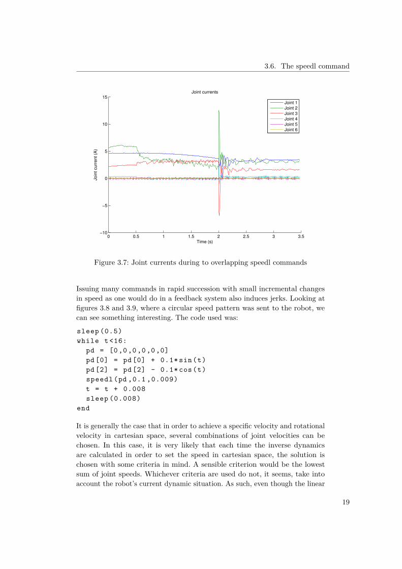
Figure 3.7: Joint currents during to overlapping speedl commands

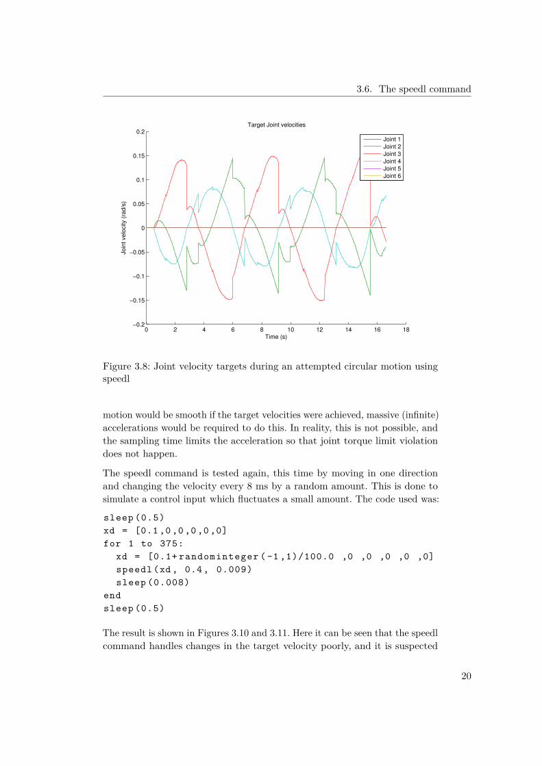
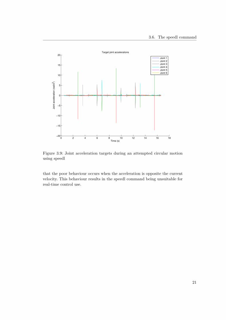
Issuing many commands in rapid succession with small incremental changesin speed as one would do in a feedback system also induces jerks. Looking atfigures 3.8 and 3.9, where a circular speed pattern was sent to the robot, wecan see something interesting. The code used was:

sleep (0.5)while t <16:

pd = [0 ,0 ,0 ,0 ,0 ,0]pd [0] = pd [0] + 0.1* sin(t)pd [2] = pd [2] - 0.1* cos(t)speedl (pd ,0.1 ,0.009)t = t + 0.008sleep (0.008)

end

It is generally the case that in order to achieve a specific velocity and rotationalvelocity in cartesian space, several combinations of joint velocities can bechosen. In this case, it is very likely that each time the inverse dynamicsare calculated in order to set the speed in cartesian space, the solution ischosen with some criteria in mind. A sensible criterion would be the lowestsum of joint speeds. Whichever criteria are used do not, it seems, take intoaccount the robot’s current dynamic situation. As such, even though the linear

19

3.6. The speedl command

0 2 4 6 8 10 12 14 16 18−0.2

−0.15

−0.1

−0.05

0

0.05

0.1

0.15

0.2Target Joint velocities

Time (s)

Jo

int

ve

locity (

rad

/s)

Joint 1

Joint 2

Joint 3

Joint 4

Joint 5

Joint 6

Figure 3.8: Joint velocity targets during an attempted circular motion usingspeedl

motion would be smooth if the target velocities were achieved, massive (infinite)accelerations would be required to do this. In reality, this is not possible, andthe sampling time limits the acceleration so that joint torque limit violationdoes not happen.

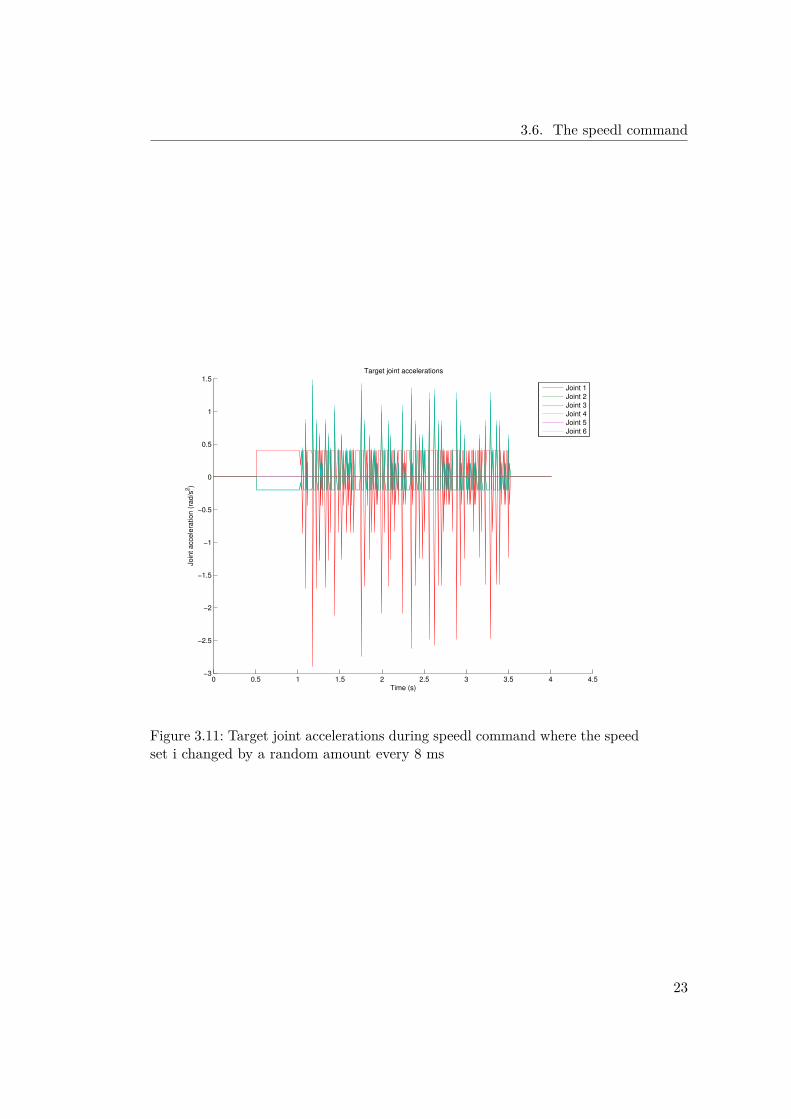
The speedl command is tested again, this time by moving in one directionand changing the velocity every 8 ms by a random amount. This is done tosimulate a control input which fluctuates a small amount. The code used was:

sleep (0.5)xd = [0.1 ,0 ,0 ,0 ,0 ,0]for 1 to 375:

xd = [0.1+ randominteger ( -1 ,1)/100.0 ,0 ,0 ,0 ,0 ,0]speedl (xd , 0.4, 0.009)sleep (0.008)

endsleep (0.5)

The result is shown in Figures 3.10 and 3.11. Here it can be seen that the speedlcommand handles changes in the target velocity poorly, and it is suspected

20

3.6. The speedl command

0 2 4 6 8 10 12 14 16 18−20

−15

−10

−5

0

5

10

15

20Target joint accelerations

Time (s)

Join

t accele

ration (

rad/s

2)

Joint 1

Joint 2

Joint 3

Joint 4

Joint 5

Joint 6

Figure 3.9: Joint acceleration targets during an attempted circular motionusing speedl

that the poor behaviour occurs when the acceleration is opposite the currentvelocity. This behaviour results in the speedl command being unsuitable forreal-time control use.

21

3.6. The speedl command

0 0.5 1 1.5 2 2.5 3 3.5 4 4.5−0.15

−0.1

−0.05

0

0.05

0.1

0.15

0.2

0.25Target Joint velocities

Time (s)

Join

t velo

city (

rad/s

)

Joint 1

Joint 2

Joint 3

Joint 4

Joint 5

Joint 6

Figure 3.10: Target joint velocities during speedl command where the speedset i changed by a random amount every 8 ms

22

3.6. The speedl command

0 0.5 1 1.5 2 2.5 3 3.5 4 4.5−3

−2.5

−2

−1.5

−1

−0.5

0

0.5

1

1.5Target joint accelerations

Time (s)

Jo

int

acce

lera

tio

n (

rad

/s2)

Joint 1

Joint 2

Joint 3

Joint 4

Joint 5

Joint 6

Figure 3.11: Target joint accelerations during speedl command where the speedset i changed by a random amount every 8 ms

23

3.7. The stopj command

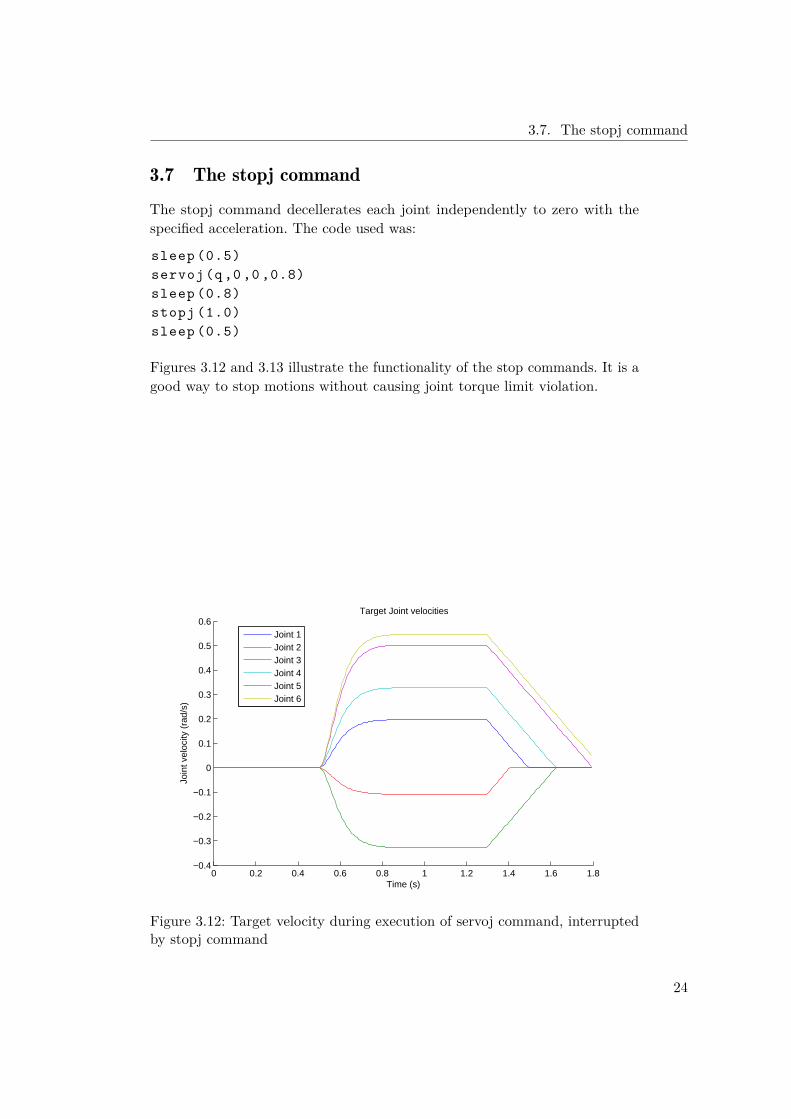
3.7 The stopj commandThe stopj command decellerates each joint independently to zero with thespecified acceleration. The code used was:

sleep (0.5)servoj (q ,0 ,0 ,0.8)sleep (0.8)stopj (1.0)sleep (0.5)

Figures 3.12 and 3.13 illustrate the functionality of the stop commands. It is agood way to stop motions without causing joint torque limit violation.

0 0.2 0.4 0.6 0.8 1 1.2 1.4 1.6 1.8−0.4

−0.3

−0.2

−0.1

0

0.1

0.2

0.3

0.4

0.5

0.6Target Joint velocities

Time (s)

Join

t vel

ocity

(ra

d/s)

Joint 1Joint 2Joint 3Joint 4Joint 5Joint 6

Figure 3.12: Target velocity during execution of servoj command, interruptedby stopj command

24

3.8. The stopl command

0 0.2 0.4 0.6 0.8 1 1.2 1.4 1.6 1.8−3

−2

−1

0

1

2

3

4Target joint accelerations

Time (s)

Join

t acc

eler

atio

n (r

ad/s

2 )

Joint 1Joint 2Joint 3Joint 4Joint 5Joint 6

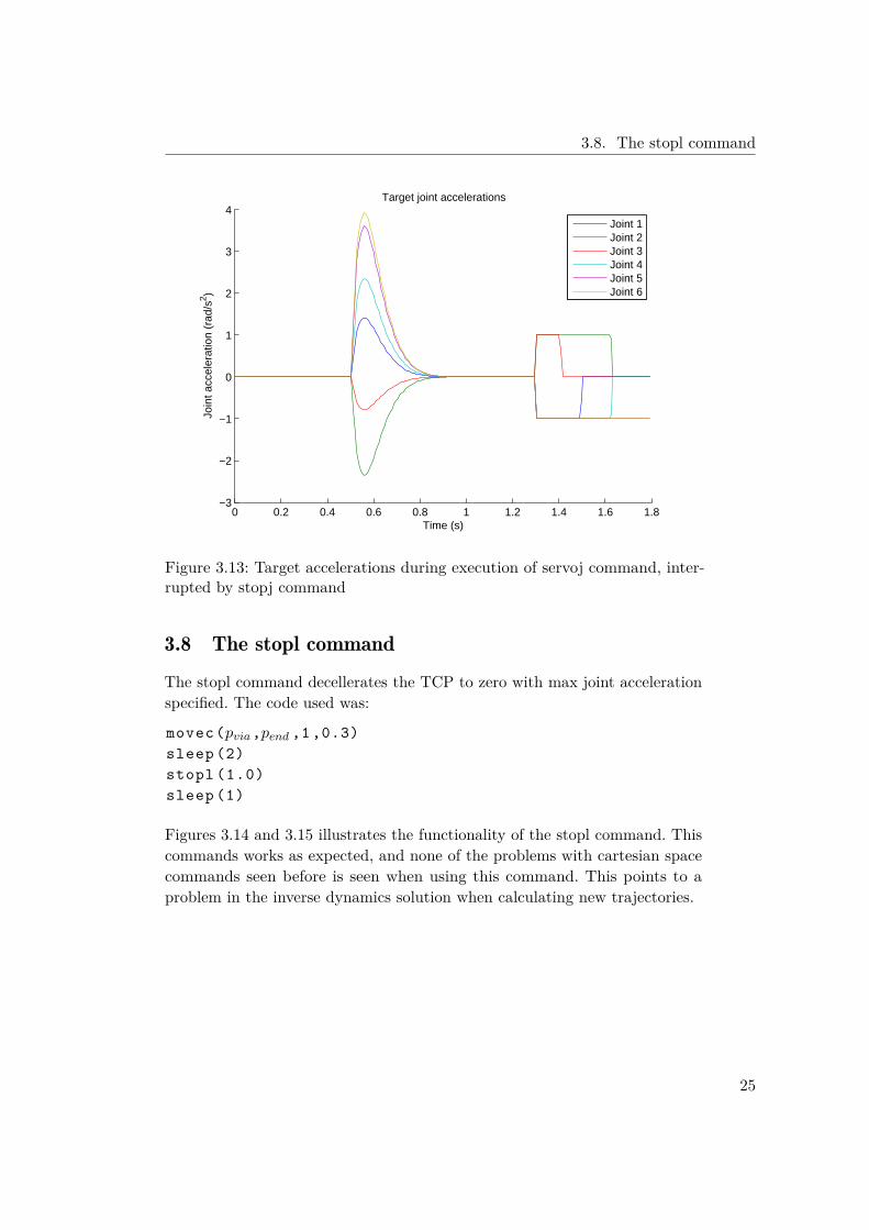
Figure 3.13: Target accelerations during execution of servoj command, inter-rupted by stopj command

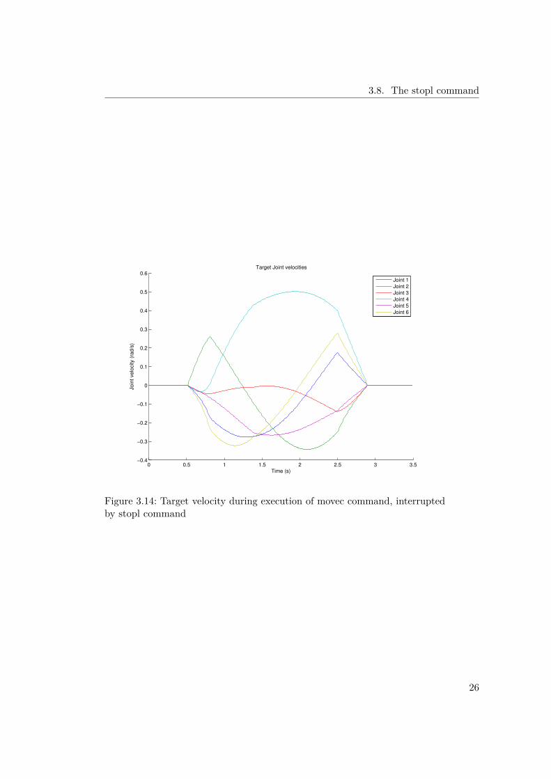
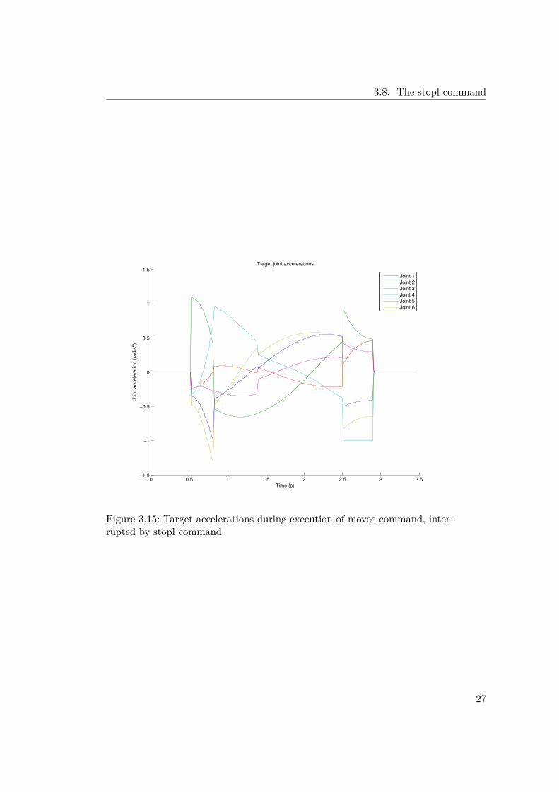
3.8 The stopl commandThe stopl command decellerates the TCP to zero with max joint accelerationspecified. The code used was:

movec(pvia,pend ,1 ,0.3)sleep (2)stopl (1.0)sleep (1)

Figures 3.14 and 3.15 illustrates the functionality of the stopl command. Thiscommands works as expected, and none of the problems with cartesian spacecommands seen before is seen when using this command. This points to aproblem in the inverse dynamics solution when calculating new trajectories.

25

3.8. The stopl command

0 0.5 1 1.5 2 2.5 3 3.5−0.4

−0.3

−0.2

−0.1

0

0.1

0.2

0.3

0.4

0.5

0.6Target Joint velocities

Time (s)

Jo

int

ve

locity (

rad

/s)

Joint 1

Joint 2

Joint 3

Joint 4

Joint 5

Joint 6

Figure 3.14: Target velocity during execution of movec command, interruptedby stopl command

26

3.8. The stopl command

0 0.5 1 1.5 2 2.5 3 3.5−1.5

−1

−0.5

0

0.5

1

1.5Target joint accelerations

Time (s)

Join

t accele

ration (

rad/s

2)

Joint 1

Joint 2

Joint 3

Joint 4

Joint 5

Joint 6

Figure 3.15: Target accelerations during execution of movec command, inter-rupted by stopl command

27

4 Conclusion

From tests we have seen that URScript and the URController is designedfor open-loop point-to-point control. The only command that can handleinterruptions is speedj, all other commands handle interruption poorly. Thebandwidth with which one can expect to control the robot is determined bythe 24ms round-trip time.

28