Uns~eady-~tate Pre~s~re Distributions Created by a Well WIth a SIngle InfInIte-Conductivity Vertical Fracture

ALAIN C. GRINGARTEN* MEMBER SPE-AIME

HENRY J. RAMEY, JR. R. RAGHAVAN"

MEMBERS SPE-AIME

INTRODUCTION

During the last few years, there has been an explosion of information in the field of well-test analysis. Because of increased physical under­standing of transient fluid flow, it is possible to

analyze t.l:ie entire pressure history of a well test not just long-time data as in conventional analysis.i It is now often possible to specify the time of beginning of the correct semilog straight line and determine whether the correct straight line has been properly identified. It is also possible to identify well bore storage effects, and the nature of wellbore stimulation as to permeability improvement, or fractU"ring, and to quantitatively analyze. those effects.

Such accomplishments have been augmented by attempts to understand the short-time pressure data from well testing - data that were often classified as too complex for analysis. One recent study of short-time pressure behavior2 showed that it was important to specify the physical nature of the stimulation in considering the behavior of a stimulated well. That is, stating that the van Everdingen - Hurst infinitesimal skin effect was negati ve was not sufficient to define short-time well behavior. For instance, acidized (but not acid-fractured) and hydraulically fractured wells might not necessarily exhibit the same behavior at early times, even though they could possess the same value of negative skin effect.

In the same manner, hydraulic fracturing leading to horizontal or vertical fractures could produce the same skin effect, but with possibly different short­time pressure data. This could then provide a way to determine the orientation of fractures created by this type of well stimulation. In fact, it is generally agreed that hydraulic fracturing usually results in one vertical fracture, the plane of which includes

Original manuscript received in Society of Petroleum Engineers office June 12. 1972. Revised manuscript received Dec 18 1973. Paper (SPE 4051) was presented at the SPE-AIME '47th Annual Fall Meeting. held In San Antonio. Tex .• Oct. 8-1 I. 1972. © Copyright 1974 .Amerlcan Institute of Mining, Metallurgical. and Petroleum Engineers, Inc.

.:NOw with French Geologlcal Bureau, Orleans. France. INow with Amoco Production Co., Tulsa. Okla. References listed at end oC peper.

U. OF CALIFORNIA AT BERKELEY BERKELEY, CALIF.

STANFORD U. STANFORD, CALIF.

the wellbore. Most studies of the flow behavior for a fractured well consider vertical fractures only.3- 11

Yet it is also agreed that horizontal fractures could occur in shallow formations. Furthermore, It wo~ld appear that notch-fracturing would lead to hOClzontal fractures. Surprisingly, no detailed study of ~e horizontal fracture case had been performed untIl recently.12 A solution to this problem was presented by Gringarten and Ramey.13 In the course of their s~dy, it was found that a large variety of new tranSIent pressure behavior solutions useful in well and reservoir analysis could be constructed from instantaneous Green's functions. 14 Possi­bilities included a well with a single vertical ~racture in an infinite reservoir, or at any location In a rectangle.

Although similar cases had been studied before by van Everdingen and Meyer,ll and by Russell and Truitt,S there were confusing differences in their respective results, and small inconsistencies between the cases of Ref. 8 made short-time analysis impossible. Both explicit and implicit finite-difference solutions and finite-element solutions were made for the vertical fracture case of Russell and Truitt in an attempt to eliminate differences between Refs. 8 and 11, and internal differences between cases in Ref. 8. It was not pos sible to reach satisfactory conclusions for the short-time performance region with even very long computer runs with either finite-difference or finite-element 12 programs. For this reason, it was decided to evaluate analytical solutions to provide a sound basis for short-time analysis of field data. In the course of the work, to provide a direct comparison with the Russell and Truitt data it became necessary to develop analytical solutions for fracture cases in which the fluid entry flux along the fracture caused a constant pressure along the fracture (infinite fracture conductivity). It also appeared worthwhile to evaluate the new solutions so that vertical fracture behavior could be compared with horizontal fracture behavior in infinite reservoirs. The new solutions for vertically fractured wells are especially useful for short-time or type-curve analysis. Such an analysis can provide information concerning permeabilities, fracture

3-&7

length, and distance to a symmetrical drainage limit. Combination of short-time analy~is with older conventional semilog analytical methods permits an extraordinary confidence level concerning the analysis of field data.

VER TICALL Y FRACTURED WELL IN AN INFINITE RESERVOIR

We model a plane (zero-thickness) vertical fracture totally penetrating a horizontal, homogeneous, and isotropic reservoir initially at constant 'pressure. At time zero, a single-phase, slightly compressible fluid flows from the reservoir into the fracture at a constant total rate. The producing pressure is uniform over the fracture (infinite fracture conductivity). The pressure remains constant and equal to the initial pressure as distance from the well becomes infinitely large (infinite reservoir).

An analytical expression for the pressure di stribution created by the plane vertical fracture may be obtained by the Green's function and product s.olution method,22 using source functions presented by Gringarten and Ramey)4 The condition of uniform pressure over the fracture at all times is satisfied, as indicated in Ref. 14, by dividing the half-fracture length xI into M segments of length x/ 1M, each with a UnIform flux per unit area, qm' (m = I,M). The first segment extends from 0 to x/1M, the second segment from x/1M to 2x/IM, the mth segment from [em -1)Xj JIM to mxllM, and ~he l~st segment from [(M -I)IM]x1 to xI' as shown In FIg. 1. The qm (m = I,M) are determined by equating the pressure drops at the center of the segments, which provide (M -1) equations, the mth equation being obtained from the condition of constant total production rate at all times:

r bp (2~~1 xf, 0, t) = Ap (2j+1 X Ll 2M f'

0, t) j = I, }i-I . (1)

M

2 L = . . . . . (2)

m=1

The pressure drop created by the fracture IS obtained from Ref. 14, Table 5:

3411

I <pc

jIDXf

M M

It I ~(T) o m=1 (m-I)x

f M

J-:f

exp

(m-I) M Xf

dT

[-

4nTj(t-T)

M

L qm(T)

m=1

2 2] (x-xv;) + y

4n(t-T) dx v;

. . . . . . . . . . (3)

J?e coordinate system in Fig. 1 and Eq. 3 is different from that of Ref. 14, however. A similar scheme has been used by Muskat15 for the steady­state pressure distribution created by a partially penetrating well, and has been suggested by Burns 16

for unsteady state. In the unsteady state, however, the method seems impractical: it was expected _ and confirmed from a numerical simulation 21 _ that the flux per unit area of fracture is not constant but varies in time. A system of M equations and M unknowns as represented by Eqs. 1 and 2 should thus be solved at each value of time.

Actually, this is not true practically, and the pressure distribution can be obtained by solving the system of equations only once. The flux distribution in the fracture at various times as obtained from a numerical simulation, is show~ in Fig. 2. It can be seen that the flux distribution is uniform at very early times, then it changes and finally it reaches a steady state at some ext~nded time, after which flow entering the fracture stabilizes. The pressure during the stabilized flow period is independent of the flux distribution history, and is the same as if the flux distribution had been equal to the final stabilized flux di stribution at all times.

An analog to this interesting and useful fact

y

o

Possible boundory conditions ;i (0) Uniform flux

(, (b) '0';0;" "od,";,;',

Xf x m-I m M Xf M Xf

FIG. 1 - VERTICAL FRACTURE IN AN INFINITE RESERVOIR.

SOCIETY OF PETROLELM E:'iGI:'I"EERS JOUR:'I"AL

occurs in the case of flow to a constant-rate well with wellbore storage. Wellbore storage causes the sand-face production rate to change as a function of time initially. But after some initial period, the sand-face rate reaches the constant surface rate (within a specified percentage), and thereafter the producing pressure is equal to that of a well whose sand-face rate had been constant from the start of production. The pressure is independent of the production history! The same son of observation was made in another reservoir problem by Carter and Tracy.23

By solving the system of Eqs. 1 and 2 for the stabilized flux distribution one can obtain a long­time solution for the pressure, whereas an early-time solution can be obtained by assuming uniform flux. We shall show that these also provide an excellent approximation for the pressure distribution at all times.

EARLY-TIME SOLUTION

Integrating Eq. 3 with respect to x w' the dimensionless pressure drop can be written as

M

m=1

C~(::)hxf) [erf m

~ + M

.!t-t' )D

m-l m

-erf ~+M

- erf ~- M

2/(t-t' >0 2/(t-t' )D

m-l ] dt' ~- --+ erf

M D 1/2

2/(t:-t')D 4 [(t-t' )D/ TI ]

. . . . . . . . . . . (4)

The dimensionless space and time variables in Eq. 4 are based on the fracture half-length XI'

X XU = x

f

y =.L., . ....... (5) D Xf

and the dimensionless time and the dimensionless pressure drop are, respectively,

kt 2 ' ............. (6)

$\..Icxf

and

_ 2TIkh ( PD (xD ' Y D' t D) - q \..I Pi - P x, Y, t) .

f

AUGU~T. 197·'

.(7)

At very early times, the expression

..s..m ~ .:-. ~1

erf 2/(t-t' )

D

becomes constant when tD is small enough.1 4 (The

constant is 2 if (m -l)/M < Ix DI < m/M; unity if IXD I '" (m-l)/M or IXDI '" m/M; and zero if IXDI < (m-l)/M or IXD I > m/M.) Therefore, at very early times the system given by Eqs. 1 and 2 reduces to

2qj +1 (t~)hXf

qf

dt' D

1/2 ' 4 [(t-t' )D/ TI ]

_ j=l, M-l ........ (8)

M

L M, m=1

. . . . . . . (9)

which yields

j=I,M .

As indicated by the numerical model, the flux must be uniform over the fracture at very early times, and the early-time solution for the pressure drop function is

7

6

5

4 M

" Ea '" 3 N

Stabilized DISfribution to_t

2

0.1

OL-____ ~ ______ -L ______ ~ ______ L_ ____ ~

05 0.6 07 08 0.9 1.0

Dimensionless distance, "0 a Jt Ix,

FIG. 2 - FLUX DISTRIBUTION AT VARIOUS TIMES ALONG AN INFINITE -CONDUCTIVITY VERTICAL

FRACTURE (NUMERICAL MODEL).

349

- 1Ynl erfc <IYnl/2~) ... (10)

Pn<lxnl>l,yn,tn) = 0

and, along the fracture,

which is the conventional result for flow in a linear system. In this case, there is flow into both sides of the fracture.

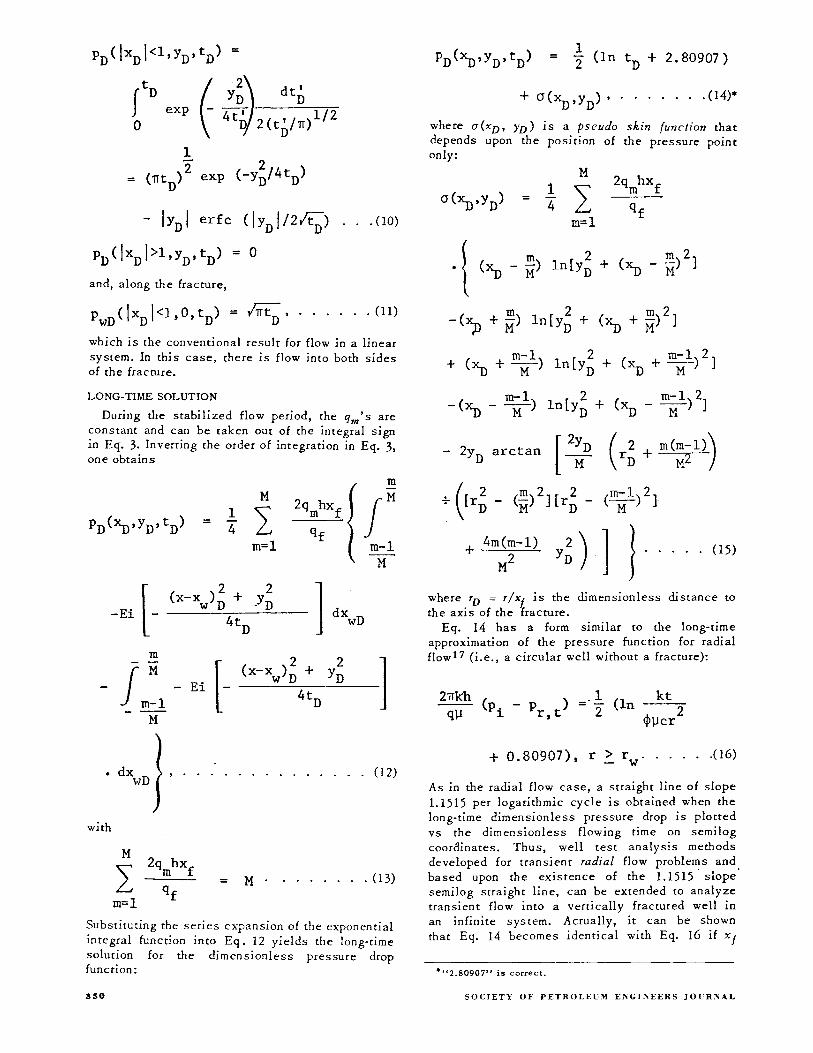
LONG-TIME SOLUTION

During the stabilized flow period, the qm's are constant and can be taken out of the integral sign in Eq. 3. Inverting the order of integration in Eq. 3, one obtains

=

-E1 [-

m

j :1 - Ei

- --lof

dx"n) , ..

with

M 2Qmhxf

I Qf m=1

1 4

[-

M

I m=1

2q~:Xf [j= m-l

1-1

. . . . . . . . . . . (12)

= M . . ...... (13)

Substituting the series expansion of the exponential integral function into Eq. 12 yields the long-time solution for the dimensionless pressure drop function:

S50

1 2 (In tn + 2.80907)

. . . . (14)·

where a(xD' YD) is a pseudo skin function that depends upon the position of the pressure point only:

= 1 4

M

I m=1

~ m 2 ( .!!!) 2] "l (~- M) In[Yn + ~ - H

m 2 m 2 -(~ + M) In[Yn + (~ + M) ]

m-I 2 m-I 2 + (~ + M) In[Yn + (~ + M) ]

( 2 + ID(m-I») rn M2

+ 4m(m-l) 2)] ~ M2 Yn J ..... (15)

where TD = T/X[ is the dimensionless distance to

the axis of the fracture. Eq. 14 has a form similar to the long-time

approximation of the pressure function for radial flow 17 (i.e., a circular well without a fracture):

=.1 (In 2

kt 2

¢~cr

+ 0.80907), r > rw' . . . . .(16)

As in the radial flow case, a straight line of slope 1.1515 per logarithmic cycle is obtained when the long-time dimensionless pressure drop is plotted vs the dimensionless flowing time on semi log coordinates. Thus, well test analysis methods developed for transient radial flow problems and. based upon the existence of the 1.1515 slope semilog straight line, can be extended to analyze transient flow into a vertically fractured well in an infinite system. Actually, it can be shown that Eq. 14 becomes identical with Eq. 16 if x f

·"2.80907" is correct.

SOCIETY OF PETROLElj:\l E1\'GI:-iEERS JOl:R:-iAL

tends to zero, of if r becomes very large. The qm' S (m -I,M) in Eq. 15 are obtained by

solving the system of equations represented by Eqs. 1 and 2, which now reduces to

2j-1 a ( 21-1 ' 0)

2j+1 a ( 2H ' 0)

j = 1, :1-1 ' . . . . . (17)

}1

I = M. . .. (18)

m=l

UNIFORM FLUX VERTICAL FRACTURE

This case corresponds to M = 1 and represents a first approximation of the· behavior of a vertically fractured well. At early times, however, it is the exact solution.

The corresponding form of Eq. 4 is

... (19)

Eq. 19 cannot be expressed in terms of tabulated functions, and must be evaluated with a computer, except in the plane of the fracture (Yv = 0), where it becomes

+ erf 1+~ 1 2~

(1:'1» E1 [_

1 ( ) 1/2 [ f 1-~ 2 TItn er----2~

4

(1_~)2 ]

4tn

. . . .(20)

Eq. 20 shows that pressure will vary along the fracture length (except at early times), which would not be true if the fracture had infinite conductivity. However, the pressure drop along the fracture is low, and the uniform flux condition gives the appearance of a high, but not infinite, fracture conducti vi ty. Some field data appear to match thi s solution better than the infinite-conductivity solution.

AUGliST.197.

One useful the pressure

(xV = 0, tv =

expression for well test analysis is drop on the aXIs of the fracture

0):

=

_ .! Ei ( __ 1 ) 2 4tn

(21)

PwD(tD ) has been listed vs tD in Table 1, and plotted in Figs. 3 and 4 as the (xe/x/ = (0) curve.

Approximating forms of Eq. 19 at small and large values of time are the same as obtained in the previous section. The sigma pseudo skin function for the long-time approximation, Eq. 15, simplifies to

i .. I

8

- 2y n

sl~ 6 . -NeT

• 4 o

a.'

2 ApprOXimate End of Linear Flow Perlod-,

• . (22)

10 10'

FIG. 3-pwv VS tv FOR A UNIFORM FLUX VERTICAL FRACTURE.

i 0-I

0:

~I~ . -Ncr

0

c.'

10

Uniform flUIl

frOClure

t -o

ApprOlimale slod of semi-log SfrO'Qhl line

('" "151/109-)

kl

4>I'Clf'

FIG. 4-PwD VS 'D FOR A UNIFORM FLUX VERTICAL FRACTURE.

3S1

and in the plane of the fracture,

(10(xO

'O) = -} [(l-xO) Inll-xol

+ (l~) In !l+~ I] .(23)

TABLE 1 - PwD FOR A VERTICALLY FRACTURED WELL IN AN INFINITE RESERVOIR

1. OE-02 1. 5E-02 2.0E-02 3.0E-02 4.0E-02 5.0E-02 6.0E-02 8.0E-02

1. OE-01 1. 5E-01 2.0E-01 3.0E-01 4.0E-01 5.0E-0l 6.0E-01 8.0E-01

1. OE+OO 1. 5E+00 2.0E+00 3.0E+OO 4.0E+OO 5.0E+OO 6.0E+00 8.0E+OO

1. OE+01 1. 5E+01 2.0E+01 3.0E+01 4.0E+01 5.0E+01 6.0E+01 8.0E+01

1. OE+02 1. 5E+02 2.0E+02 3.0E+02 4.0E+02 5.0E+02 6.0E+02 8.0E+02

1. OE+03 1. 5E+03 2.0E+03 3.0E+03 4.0E+03 5.0E+03 6.0E+03 8.0E+03

352

Uniform flux

0.1772 0.2171 0.2507 0.3070 0.3545 0.3963 0.4340 0.5007

0.5587 0.6790 0.7756 0.9261 1. 0417 1.1355 1. 2145 1. 3427

1.4447 1. 6344 1. 7716 1. 9676 2.1080 2.2175 2.3073 2.4494

2.5600 2.7613 2.9045 3.1065 3.2500 3.3614 3.4524 3.5961

3.7075 3.9101 4.0539 4.2566 4.4004 4.5119 4.6031 4.7469

4.8584 5.0612 5.2050 5.4077 5.5516 5.6631 5.7543 5.8981

Infinite Conductivity

0.1765 0: 2145 0.2456 0.2955 0.3356 0.3697 0.3996 0.4509

0.4945 0.5833 0.6549 0.7691 0.8603 0.9367 1. 0027 1.1129

1. 2030 1. 3754 1. 5032 1. 6894 1. 8248 1.9312 2.0189 2.1583

2.2673 2.4664 2.6085 2.8094 2.9524 3.0634 3.1542 3.2976

3.4089 3.6113 3.7549 3.9575 4.1012 4.2127 4.3039 4.4477

4.5592 4.7619 4.9057 5.1084 5.2523 5.3638 5.4550 5.5988

the long-time approximation applies within 1 percent when

. . . . . . . (24)

IN FINITE-CONDUCTIVITY VERTICAL FRACTURE

The system of linear equations given by Eqs. 17 and 18 must be solved for 2qmhx/1 qt' which represents the ratio of the flux per unit length in the mth segment, qm' to the flux per unit length in the uniform flux fracture case, q/2hx/. The stabili zed value of 2qmhx/1 q/ along the half-fracture length is shown in Fig. 5. Although uniform pressure in the fracture can be obtained with as little as 10 segments, it is necessary to use enough divisions obtain a stabilized value of 0D(!xD!<I, 0) = 0wD in the fracture, as indicated by Fig. 6. The change in 0wD is less than 5 x 10-5 when the number of fracture segments is increased from 59 to 60. In this study, we have used 90 segments to obtain a stabilized value of 0wD in the fracture equal to

-0.305. This value of 0wD can be guaranteed to

within 0.1 percent. The precision of determinatiDn of the dimensionless pressure given by Eq. 14 is, of course, much higher. Eq. 14 then yields for the long-time pressure drop on the fracture,

. . (25)

The same result can be obtained in the uniform flux fracture case by measuring the pressure drop at xD = 0.732 in the fracture. This can be calculated

by substituting -0.305 for o(xD' 0) in Eq. 23. It is obvious in Fig. 7. This suggests that the pressure drop on the fracture for the infinite-conductivity fracture can be obtained from that for the uniform flux fracture. Eq. 20, with xD = 0.732. Th'e result IS

K .J::. _

E cr cr

N

FIG. 5

8

6

4

2

infinite conductivity frocture

uniform flux fractu7

OL--L __ L--L __ l-~ __ ~~--~~~

o 0.2 0.4 0.6 0.8 x

Dimensionless Distance, )(0 = Xf _ STABILIZED FLUX DISTRIBUTION ALONG

VERTICAL FRACTURE.

SOCIETY OF PETROLEI'M E:\'GI:\EERS JOI'R:\'AL

_ 0.433 Ei (_ O. ~~O) ....... (26)

Eq. 26 yields the correct value of the wellbore pressure for a well with an infinite-conductivity

0 b~

-0.1 -

c 0

U C ::I

I.J.. c

oX

'" 0 -0.2 '0 ::I Q)

'" a.

~ 0

.D

a:; 3:

-0.3 - -

I I I I o 20 40 60 80 100

number of segments in fracture, m

FIG. 6-CONVERGENCE OF THE WELLBORE PSEUDO SKIN FUNCTION a wO (INFINITE - CONDUCTIVITY

FRACTURE).

or-~~'------'------'------'------'------'

'!. a.Ds-O.30~

~ -0.5

b infinite conductivity fracture

c -1 0 fracture O](IS

u C

~

~ -1.5

.. 0 '0 -2 " .. .. 0-

-2.5 0 2 3

Dimensionless Distance, x :: L o xf

FIG. 7-PSEUDO SKIN FUNCTION VS DIMENSIONLESS DISTANCE.

AUGUST.197·'

vertical fracture, at early and long times. It can be assumed that it also yields the correct pressure values during the transition period. A similar result (xD = 0.75) has been obtained by Muskat15 for a well with partial penetration at steady state. PwD(tD) from Eq. 26 has been listed vs tD in Table 1, and graphed in Figs. 8 and 9, where it corresponds to the (xe/xi = 00) curve.

VERTICALLY FRACTURED WELL IN A RECTANGULAR CLOSED RESERVOIR

When a reservoir is in an early stage of depletion, the production of a particular well is not perturbed by the existence of other wells or by boundary effects. After a while this is no longer true, and a new solution must be developed that considers the reservoir boundaries or the effect of the other wells.

Fig. 10 presents a schematic of a vertically fractured well in a rectangular, closed drainage system. Two types of fracture will be considered -- uniform flux and infinite conductivity -- but, as in the infinite-reservoir case, it is only necessary to derive the dimensionless pressure drop for the uniform flux fracture. This is obtained immediately

i C1 I

10 -- ~ • ~" "'I "T , ""I

c;r .. , .. " .... ••• / In'lntte conducflvlf)'

frocture

". -h .. -

8

;1" 6 . -NeT

o c,"

4 End of linear flow period

for *>1

2 End of linear flow period

for *~I Approximate slorr of semi-log

slroighl line (m' 1.15Vlog-)

~O'2'~-'~'~ ~I~ _ •. ~..L~~~ .• ~. ~ 10'

t ____ kt __ _

o .I"Cxf'

FIG. 8-pwo VS to FOR AN INFINITE-CONDUCTIVITY VERTICAL FRACTURE.

.. Q.

S 10

!il" ~ -N'"

o c.,"

2,.-

Inflnile conduchvrly 'rae lure

FIG. 9-pwo VS to FOR AN INFINITE-CONDUCTIVITY VERTICAL FRACTURE.

353

by mean s of the Green's function and product

solution method (see Ref. 14). The result is

2n ItDA 00

X L [1 + 2 ~1 PD(~'Y ,tDA) = e e 0

2 2 X

t~A) cos Yw

• exp (-e

n 1T n1T 2y Ye e

00

Y +Y] [1 ~ exp (-2 2

'01 + 2 n 1T • cos n1T -2-

Ye n=l X

f sin n1T 2x X

Ye t~A ) xe

n1T

• cos n1T

xf

2x e

e W cos n1T 2x

e

, ....... (27)

where tDA represents the dimensionless time based on the drainage area:

kt ..... (28)

The pressure drop on the fracture for a vertical fracture at the center of a square (xe == Ye and x w ==

Y w ) is then given by

00

.----.

I tDA r 21T II + 2

o '>

L.J n=l

00

(1 + 2 ~1 ( 2 2 I ) exp -4n 1T tDA

sin x

f n1T

X e

xf

n1T X e

.. (29)

The pressure drops on the fracture for a uniform flux fracture and for an infinite-conductivity fracture are obtained by evaluating Eq. 29 at xD == 0 and xD == 0.732, respectively. The choice of the same point as in the infinite case leads to reasonable results and can be justified a posteriori by the method of desuperposition, presented later in this paper. Numerical values of the dimensionless

354

pressure drop from Eq. 29 are listed vs tDA in Tables 2 and 3, and have been plotted vs t D (not tDA ) in Figs. 3 and 4 and Figs. 8 and 9, respectively, for various values of the xe/xi ratio. This ratio is used instead of Russell and Truitt's8 fracture penetration ratio xi/xe because the limiting case of a vertical fracture in a square reservoir is a vertical fracture in an infinite reservoir (Figs. 3, 4, 8, and 9), which correspond to xe/xi == 00,

whereas a zero fracture penetration ratio (xjlxe = 0) corresponds to an unfractured well in a square reservoir, which is a different problem.

Three different flow periods can be characterized for both types of fractures: a linear flow period occurs at early times. This corresponds to the one-half slope straight line in log-log coordinates (Figs. 4 and 9). After a period of transition, there is a pseudoradial flow period corresponding to the semilog straight line (Figs. 3 and 8). After a second period of transition, pseudosteady state occurs, which is characterized by an approximate unit slope straight line in log-log coordinates. Depending upon xe1x/, one or more of these different flow periods may be missing; in the total fracture penetration case (xe/xi == 1), for instance, the first transition period and the pseudoradial period do not appear, whereas only the pseudoradial period is missing for values of xe/xi between J and 3 (uniform flux fracture), or 1 and 5 (infinite-conductivity fracture).

DISCUSSION OF VERTICAL FRACTURE SOLUTIONS

A comparison has been made in Table 4, and in Figs. 11 and 12 between the subject analytical solution for the infinite-conductivity fracture and Russell and Truitt's results.8 As can be seen from Figs. 11 and 12, the smaller the xe/xl' the closer the two solutions become at long times. The over-all agreement is good, in view of the fact that the Russell and Truitt solution is an explicit finite­difference solution for a very difficult problem. The total fracture penetration cases (xe/xi == 1) agree exactly at all times. None of the Russell-Truitt curves, however, produce the 1.1515 slope semilog

y

Possible boundory conditions

(0) uniform flux

(b) infinite conductivity

x

FIG. IO-VERTICAL FRACTURE IN A RECTANGULAR RESERVOIR.

SOCIETY OF PETROLEUM E~GI~EERS JOt:R~AL

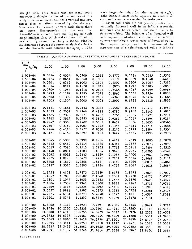
straight line. This result was for many years erroneously thought by one of the authors of this study to be an inherent result of a vertical fracture, rather than an effect caused by the drainage boundaries. Furthermore, at very early times there are some discrepancies In the way the Russell-Truitt curves leave the log-log half-unit slope straight line, which makes them difficult to use with type-curve matching methods. Finally, the difference between the current analytical solution and the Russell-Truitt solution for xe / x f = 10 is

much larger than that for other values of x e/x f' This Russell-Truitt case appears to contain an error and is not recommended for further use.

Russell and Truitt did not provide results for a vertically fractured well in an infinite reservoir, but such can be extracted from their results by desuperposition. The behavior of a fractured well in a square is identical with that of an infinite system containing a square array of fractured wells. The square array could be constructed by superposi tion of single fractured wells in infinite

TABLE 2 - PwD FOR A UNIFORM FLUX VERTICAL FRACTURE AT THE CENTER OF A SQUARE

1. 00E-04 1. 50E-04 2.00E-04 3.00E-04 4.00E-04 5.00E-04 6.00E-04 8.00E-04

1. 00E-03 1. 50E-03 2.00E-03 3.00E-03 4.00E-03 5.00E-03 6.00E-03 8.00E-03

1. 00E-02 1. 50E-02 2.00E-02 3.00E-02 4.00E-02 5.00E-02 6.00E-02 8.00E-02

1. 00E-01 1. 50E-01 2.00E-01 3.00E-01 4.00E-01 5.00E-01 6.00E-01 8.00E-01

1.00E+00 1.50E+00 2.00E+00 3.00E+00 4.00E+00 5.00EtOO 6.00E+OO 8.00E+00

"l'Gl!~T. 197.

1.00

0.0354 0.0434 0.0501 0.0614 0.0709 0.0793 0.0868 0.1003

0.1121 0.1373 0.1585 0.1942 0.2242 0.2507 0.2746 0.3171

0.3545 0.4342 0.5013 0.6140 0.7092 0.7935 0.8708 1.0127

1.1458 1. 4652 1. 7801 2.4086 3.0369 3.6652 4.2935 5.5501

6.8068 9.9484

13.0900 19.3732 25.6563 31. 9395 38.2227 50.7891

1.50

0.0532 0.0651 0.0752 0.0921 0.1063 0.1189 0.1302 0.1504

0.1681 0.2059 0.2378 0.2912 0.3363 0.3760 0.4118 0.4752

0.5306 0.6460 0.7393 0.8861 1.0011 1.0973 1.1819 1. 3315

1. 4678 1. 7895 2.1047 2.7332 3.3615 3.9898 4.6181 5.8748

7.1314 10.2730 13.4146 19.6978 25.9810 32.3641 38.5473 51.1137

2.00

0.0709 0.0868 0.1003 0.1228 0.1418 0.1585 0.1737 0.2005

0.2242 0.2746 0.3171 0.3883 0.4482 0.5007 0.5477 0.6297

0.6999 0.8414 0.9515 1.1183 1. 2443 1. 3470 1. 4356 1. 5893

1. 7273 2.0502 2.3655 2.9941 3.6224 4.2507 4.8790 6.1357

7.3923 10.5339 13.6755 19.9587 26.2418 32.5250 38.8082 51. 3746

3.00

0.1063 0.1302 0.1504 0.1842 0.2127 0.2378 0.2605 0.3008

0.3363 0.4118 0.4752 0.5801 0.6661 0.7392 0.8030 0.9103

0.9986 1.1686 1. 2953 1. 4804 1. 6159 1. 7241 1. 8161 1. 9734

2.1129 2.4368 2.7523 3.3808 4.0092 4.6375 5.2658 6.5224

7.7791 10.9207 14.0623 20.3455 26.6286 32.9118 39.1950 51.7614

5.00

0.1772 0.2171 0.2507 0.3070 0.3545 0.3962 0.4340 0.5007

0.5587 0.6790 0.7756 0.9261 1.0417 1.1355 1. 2145 1. 3427

1. 4447 1. 6344 1. 7716 1. 9676 2.1086 2.2201 2.3140 2.4732

2.6136 2.9381 3.2537 3.8823 4.5106 5.1389 5.7672 7.0239

8.2805 11. 4221 14.5637 20.8469 27.1301 33.4132 39.6964 52.2628

7.00

0.2481 0.3039 0.3509 0.4297 0.4957 0.5533 0.6046 0.6933

0.7686 0.9183 1. 0334 1. 2057 1. 3336 1. 4354 1. 5199 1. 6554

1. 7619 1.9577 2.0981 2.2974 2.4400 2.5524 2.6469 2.8067

2.9473 3.2720 3.5876 4.2162 4.8445 5.4728 6.1011 7.3578

8.6144 11. 7560 14.8976 21.1808 27.4639 33.7471 40.0303 52.5967

10.00

0.3545 0.4340 0.5007 0.6105 0.6999 0.7756 0.8414 0.9515

1.0417 1. 2145 1. 3427 1. 5294 1.6650 1. 7716 1. 8594 1.9990

2.1080 2.3073 2.4495 2.6505 2.7940 2.9069 3.0016 3.1618

3.3025 3.6273 3.9429 4.5715 5.1998 5.8281 6.4564 7.7131

8.9697 12.1113 15.2529 21. 5361 27.8193 34.1024 40.3856 52.9520

15.00

0.5306 0.6460 0.7392 0.8855 0.9986 1.0908 1.1686 1. 2953

1.3963 .1.5846 1.7211 1. 9164 200565 2.1658 2.2554 2.3973

2.5078 2.7090 2.8520 3.0541 3.1980 3.3111 3.4061 3.5664

3.7072 4.0320 4.4477 4.9762 5.6045 6.2328 6.8512 8.1178

9.3744 12.5160 15.6576 21. 9408 28.2240 34.5072 40.7904 53.3567

3SS

mediums in the same way a well in a closed square was constructed by Matthews el al. IS and by Earlougher el al.l 9 We realize that the pressure drop at a great distance from a fractured well produced at constant rate is essentially identical with the pressure drop caused by an unfractured well. Thus, the behavior of a fractured well in a closed square may be approximated by generating the drainage boundaries with un fractured wells, if xe1x/ is large enough. This simple approach can also be used to extract the behavior of a fractured

well in an infinite medium from that of a fractured well in a closed square. This can be stated as follows: the PD for a fractured well in an infinite medium is equal to the PD for a fractured well in a closed square, less the P D for an unfractured well in a closed square, plus the PD for an unfractured well in an infinite medium. The method has been applied to both the current analytical solutions and Russell-Truitt solutions for an infinite-conductivity fracrure in a closed square reservoir (Table 4 and Fig. 13). The data for an unfractured well In a

TABLE 3 _ PwD FOR AN INFINITE-CONDUCTIVITY VERTICAL FRACTURE AT THE CENTER OF A SQUARE

1.00E-04 1.50E-04 2.00E-04 3.00E-04 4.00E-04 5.00E-04 6.00E-04 8.00E-04

1. 00E-03 1. 50E-03 2.00E-03 3.00E-03 4.00E-03 5.00E-03 6.00E-03 8.00E-03

1.00E-02 1. 50E-02 2.00E-02 3.00E-02 4.00E-02 5.00E-02 6.00E-02 8.00E-02

1.00E-01 1. 50E-01 2.00E-01 3.00E-01 4.00E-01 5.00E-01 6.00E-01 8.00E-01

1.00E+OO 1.50E+00 2.00E+OO 3.00E+00 4.00E+OO 5.00E+OO 6.00E+OO 8.00E+OO

SS6

1.00

0.0354 0.0434 0.0501 0.0614 0.0709 0.0793 0.0868 0.1003

0.1121 0.1373 0.1585 0.1942 0.2242 0.2507 0.2746 0.3171

0.3545 0.4342 0.5013 0.6140 0.7092 0.7935 0.8708 1. 0127

1.1458 1. 4652 1. 7801 2.4086 3.0369 3.6652 4.2935 5.5501

6.8068 9.9484

13.0900 19.3732 25.6563 31. 9395 38.2227 50.7891

1. 50

0.0532 0.0651 0.0752 0.0921 0.1063 0.1139 0.1302 0.1502

0.1676 0.2040 0.2338 0.2818 0.3204 0.3533 0.3821 0.4315

0.4735 0.5595 0.6295 0.7445 0.8406 0.9254 1.0030 1.1452

1. 2784 1. 5979 1. 9128 2.5413 3.1696 3.7979 4.4262 5.6829

6.9395 10.0811 13.2227 19.5059 25.7891 32.0722 38.3554 50.9218

2.00

0.0709 0.0868 0.1003 0.1228 0.1417 0.1582 0.1730 0.1989

0.2212 0.2671 0.3041 0.3633 0.4107 0.4509 0.4863 0.5470

0.5987 0.7043 0.7891 0.9239 1. 0316 1.1235 1.2054 1. 3521

1.4872 1. 8081 2.1231 2.7516 3.3799 4.0082 4.6366 5.8932

7.1498 10.2914 13.4330 19.7162 25.9994 32.2826 38.5658 51.1321

3.00

0.1063 0.1302 0.1502 0.1832 0.2104 0.2338 0.2545 0.2901

0.3204 0.3821 0.4315 0.5104 0.5738 0.6278 0.6753 0.7569

0.8259 0.9642 1.0718 1. 2352 1. 3592 1.4607 1.5486 1. 7015

1. 8392 2.1619 2.4772 3.1057 3.7341 4.3624 4.9907 6.2473

7.5040 10.6456 13.7872 20.0703 26.3535 32.6367 38.9199 51. 4863

5.00

0.1765 0.2145 0.2456 0.2955 0.3356 0.3697 0.3996 0.4509

0.4945 0.5833 0.6549 0.7691 0.8603 0.9367 1. 0027 1.1129

1. 2030 1. 3754 1. 5033 1. 6896 1. 8256 1. 9342 2.0264 2.1838

2.3234 2.6474 2.9629 3.5915 4.2198 4.8481 5.4764 6.7331

7.9897 11.1313 14.2729 20.5561 26.8393 33.1224 39.4056 51. 9720

7.00

0.2433 0.2928 0.3327 0.3962 0.4471 0.4904 0.5284 0.5939

0.6496 0.7631 0.8536 0.9953 1.1050 1.1947 1. 2707 1.3948

1. 4941 1.6800 1. 8152 2.0092 2.1492 2.2600 2.3536 2.5124

2.6527 2.9771 3.2926 3.9212 4.5495 5.1778 5.8061 7.0628

8.3194 11. 4610 14.6026 20.8858 27.1690 33.4521 39.7353 52.3017

10.00

0.3356 0.3996 0.4509 0.5328 0.5987 0.6549 0.7042 0.7889

0.8603 1. 0027 1.1129 1. 2792 1. 4037 1.5033 1. 5862 1. 7196

1. 8248 2.0189 2.1583 2.3567 2.4989 2.6110 2.7053 2.8649

3.0055 3.3301 3.6457 4.2743 4.9026 5.5309 6.1592 7.4159

8.6725 11. 8141 14.9557 21.2389 27.5220 33.8052 40.0884 52.6548

15.00

0.4735 0.5590 0.6278 0.7379 0.8259 0.9000 0.9642 1.0718

1.1600 1. 3296 1. 4560 1. 6405 1. 7750 1.8808 1. 9681 2.1071

2.2158 2.4146 2.5564 2.7572 2.9006 3.0133 3.1081 3.2682

3.4089 3.7337 4.0493 4.6778 5.3061 5.9345 6.5628 7.8194

9.0761 12.2177 15.3592 21. 6424 27.9256 34.2088 40.4920 53.0584

SOCIETY OF PETROLEUM EJ';GI:-;EERS JOUR:-;AL

closed square were taken from Table 1, Ref. 19. It was found that desuperposition of the analytical solution for a closed square yields a very good approximation of the analyti-cal solution for an infinite reservoir, for xelxf values of 2, 5, and 1013. This justifies a posteriori the choice of xD ==

0.732 for representing the well bore pressure for an infinite-conducti vi ty fracture in the finite-reservoir case. xelxf ratios of 10/7 and 1 gives PD values that are much too large, implying that desuperposi­tion cannot be used because the fracture is too close to the square boundary. The xelxf == 10 case yields PD values by desuperposition that are far too small. It is likely that the Russell and Truitt results have a small, almost constant error for this

case. It should be noted, however, that the Russell and Truitt desuperposed solution for an infinite reservoir does have a slope of 1.151 when plotted on semilog coordinates, although their solutions for the closed square did not.

An interesting interpretation of the behavior of a vertically fractured well can be made in terms of an equivalent unfractured system. Prats5 has shown that an infinite-conductivity vertical fracture, producing an incompressible fluid from a closed circular reservoir at steady state, is equivalent to an unfractured well with an effective radius equal to a quarter of the total fracture length, for ratios of the reservoir radius to the fracture half length greater than 2. The same is true, within 7 percent,

TABLE 4 _ COMPARISON BETWEEN ANALYTICAL AND FINITE-DIFFERENCE WELL BORE PRESSURES FOR AN INFINITE­CONDUCTIVITY VERTICAL FRACTURE AT THE CENTER OF A CLOSED SQUARE

1.0 E-04 2.0 E-04 5.0 E-04 8.0 E-04

1.0 E-03 2.0 E-03 5.0 E-03 8.0 E-03

1.0 E-02 2.0 E-02 5.0 E-02 8.0 E-02

1.0 E-01 2.0 E-01 5.0 E-01 8.0 E-01

1.0 E+OO 2.0 HOO 5.0 E+OO 8.0 HOO

1.0 E-04 2.0 E-04 5.0 E-04 8.0 E-04

1.0 E-03 2.0 E-03 5.0 E-03 8.0 E-03

1. 0 E-02 2.0 E-02 5.0 E-02 8.0 E-02

1.0 E-01 2.0 E-01 5.0 E-01 8.0 E-01

1.0 E+OO 2.0 E+OO 5.0 E+OO 8.0 E+OO

AUGUST,191·'

1 Analytical

0.0354 0.0501 0.0793 0.1003

0.1121 0.1585 0.2507 0.3171

0.3545 0.5013 0.7935 1.0127

1.1458 1. 7801 3.6652 5.5501

6.8068 13.0900 31. 9395 50.7891

10/3 Analytical

0.1181 0.1666 0.2578 0.3187

0.3514 0.4711 0.6830 0.8220

0.8958 1.1550 1.5552 1. 7984

1. 9366 2.5751 4.4602 6.3452

7.6018 13.8850 32.7345 51. 5841

Finite Dif.

0.0355 0.0501 0.0793

0.1121 0.1585 0.2507 0.3171

0.3545 0.5014 0.7936 1. 0127

1.1457 1. 7797 3.6648 5.5498

6.8064 13.0696

Finite Dif.

0.1182 0.1671 0.2463

0.3318 0.4480 0.6586 0.7951

0.8668 1.1167 1. 5045 1. 7442

1. 8817 2.5189 4.4039 6.2889

7.5455 13.8287

10/7 2 Analytical Finite Dif. Analytical Finite Oif.

0.0506 0.0506 0.0709 0.0709 0.0716 0.0716 0.1003 0.1003 0.1132 0.1107 0.1582 0.1527 0.1431 0.1989

0.1598 0.1528 0.2212 0.2092 0.2233 0.2111 0.3041 0.2870 0.3386 0.3220 0.4509 0.4326 0.4142 0.3982 0.5470 0.5306

0.4548 0.4398 0.5987 0.5836 0.6062 0.5969 0.7891 0.7755 0.8973 0.8947 1.1235 1.1051 1.1160 1.1145 1. 3521 1. 3309

1.2489 1. 2477 1.4872 1.4654 1. 8832 1.8818 2.1231 2.1003 3.7683 3.7668 4.0082 3.9853 5.6532 5.6517 5.8932 5.8702

6.9099 6.9034 7.1498 7.1269 13 .1930 13.1916 13.4330 13.4101 32.0426 32.2826 50.8922 51.1321

5 10 Analytical Finite Dif. Analytical Finite Oit.

0.1765 0.1772 0.3356 0.3545 0.2456 0.2476 0.4509 0.4715 0.3697 0.3575 0.6549 0.6395 0.4509 0.7889

0.4945 0.4780 0.8603 0.8013 0.6549 0.6390 1.1129 1.0171 0.9367 0.9164 1.5033 1. 3697 1.1129 1. 0872 1. 7196 1.5732

1.2030 1.1742 1.8248 1.6735 1.5033 1.4659 2.1583 1.9970 1. 9342 1.8894 2.6110 2.4430 2.1838 2.1372 2.8649 2.6958

2.3234 2.2766 3.0055 2.8361 2.9629 2.9154 3.6457 3.4757 4.8481 4.8004 5.5309 5.3607 6.7331 6.6853 7.4159 7.2456

7.9897 7.9419 8.6725 8.5023 14.2729 14.2252 14.9557 14.7855 33.1224 33.8052 51.9720 52.6548

351

for a compressible fluid at steady or pscudostcady state. 6 We can see that these results apply to a vertically fractured well in an infinite reservoir during the pscudoradial period, because Eq. 25 can be written as

+ 0.80907]- ...... . (30)

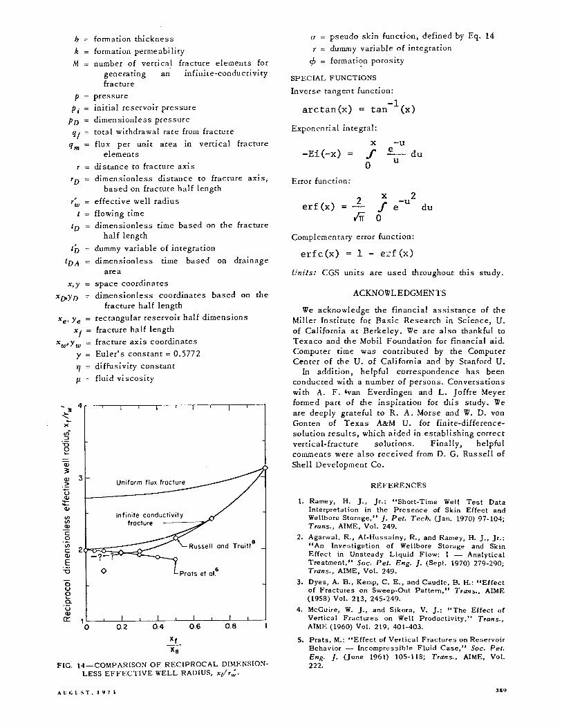
The effective well radius for an infinite-conductivity vertical fracture in an infinite reservoir is thus exactly one-fourth the total fracture length. The effective radius for an infinite-conductivity vertical fracture in a closed square reservoir at pseudosteady state may be obtained from the general pseudosteady­state depletion equation presented by Brons and Miller,20 which, 10 the present case, can be expressed as

x e , . (31)

xf

where C A is the shape factor for a well in a square, and T~ is the effective well radius. Effective radii computed from the current analytical solution and from the Russell and Truitt solution are compared in Fig. 14 with the results of Prats et al.6 for various values of xi/xe (xi/xe is used for conve­nience in this case). Surprisingly, variations of the radii as a function of x/xe are different in the Prats et al. results. Aga1O, the result for x/xe = 0.1 in Russell-Truitt' s case is inconsistent with other results.

Compari son was also made between the subi ect

i Q.

I 0:

8

~I~ 6 N'"

o 0."

4

2

10

FIG. 11 - COMPARISON OF ANALYTICAL SOLUTION AND RUSSELL AND TRUITT SOLUTION FOR AN INFINITE-CONDUCTIVITY VERTICAL FRACTURE IN

A SQUARE.

358

solution and the analytical results of van Everdingen and Meyerll for an infinite-conductivity fracture in an infinite reservoir. Although not shown, results do not compare well. The van Everdingen and Meyer solution is correct during the initial linear flow period. But it yields a semilog straight line of slope 0.576 per loglO cycle, instead of 1.151 per 10glO cycle as in the subject study, or as in the Russell and Truitt8 desuperposed solution. It is not recommended that this solution be used in the pseudoradial flow period. Either the current analytical solution, or the desuperposed Pussell­Truitt solution for a fractured well in an infinite medium may be used.

i Q.

I

$

~I~ ~ -NO"

0

a."

10

NOMENCLATURE

pseudosteady-state shape factor for a well at the center of a square l9 = 30.86

".

Infinite conduchvlty frocture

FIG. 12 - COMPARISON OF ANALYTICAL SOLUTION AND RUSSELL AND TRUITT SOLUTION FOR AN INFINITE-CONDUCTIVITY VERTICAL FRACTURE IN

8 i

Q.

• 0:

6

~I' . -",,,,

4 0

0."

2

qO··

A CLOSED SQUARE.

10-'

Analytical solution

Xth'f::CI)~

1011 Z '

10

10 kl

to - -.-","'c-•• -::.-

10'

FIG. 13 - DESUPERPOSITION OF RUSSELL AND TRUITT RESULTS TO OBTAIN A VERTICALLY FRACTURED WELL IN AN INFINITE RESERVOIR AND COMPARISON WITH THE SUBJECT ANALYTICAL SOLUTION FOR AN INFINITE-CONDUCTIVITY VERTI-

CAL FRACTURE IN AN INFINITE RESERVOIR.

SOCIETY OF PETROLEt:M E~GIl'iEERS JOURXAL

h

k

M

p

T

TD

, Tw

t' D

formation thickness

formation permeability

number of vertical fracture elements for generating an infinite-conductivity fracture

pressure

initial reservoir pressure

dimensionless pressure

total wi thdra wal ra te from fracture

flux per unit area in vertical fracture elements

distance to fracture axis

dimensionless distance to fracture aXIS, based on fracture half length

effecti ve well radius

flowing time

dimensionless time based on the fracture half length

dummy variable of integration

dimensionless tlme based on drainage area

x,y space coordinates

Xo>YD dimensionless coordinates based on the fracture half length

x e' Ye = rectangular reservoir half dimensions

x I = fracture half length

x w' y w fracture axis coordinates

y

Tf

fL

Euler's constant = 0.5772

diffusivity constant

-~ "--)(

en ::J

'6 0 .... Q)

3

4

Q) 3 >

'"5 ~ .... Q)

(/) (/)

~ c o

fluid viscosity

~ 2~~~;;(;~~~ Q) -?-? E -0 0

Xt Xe

Russell and Truitt8

FIG. 14-COMPA~ISON OF RECIPROCAL DIMENSION­LESS EFFECTIVE WELL RADIUS, xtf,,;·

A I: f; I: ST. I 9 7 l

a

T

pseudo skin function, defined by Eq. 14

dummy variable of integration

¢ formati<;>n porosity

SPECIAL FUNCTIONS

Inverse tangent function:

-1 arctan(x) = tan (x)

Exponential integral:

x -Ei(-x) = f

o

-u e

du

Error function:

erf(x) = 2

liT

x

f o

u

-u e

2 du

Complementary error function:

erfc(x) 1 - e:d (x)

Units: CGS umts are used throughout this study.

ACKNOWLEDGMENTS

We acknowledge the financial assistance of the Miller Institute for Basic Research in Sc'ience, U. of California at Berkeley. We are also thankful to Texaco and the Mobil Foundation for financial aid. Computer time was contributed by the Computer Center of the U. of California and by Stanford U.

In addition, helpful correspondence has been conducted with a number of persons. Conversations wi th A. F. 'van Everdingen and L. Joffre Meyer formed part of the inspiration for this study. We are deeply grateful to R. A. Morse and W. D. von Gonten of Texas A&M U. for finite-difference­solution results, which aided in establishing correct vertical-fracture solutions. Finally, helpful comments were also received from D. G. Russell of Shell Development Co.

REFERENCES

1. Ramey, H. J., Jr.: "Short-Time Well Test Data Interpretation in the Presence of Skin Effect and Wellbore Storage," J. Pet. Tech. (Jan. 1970) 97-104; T,ans., AIME, Vol. 249.

2. Agarwal, R., Al-Hussainy, R., and Ramey, H. J., Jr.: "An Investigation of Wellbore Storage and Skin Effect in Unsteady Liquid Flow: I - Analytical Treatment," Soc. Pet. Eng. J. (Sept. 1970) 279-290; Trans., AIME, Vol. 249.

3. Dyes, A. 8., Kemp, C. E., and Caudle, B. H.: "Effect of Fractures on Sweep-Out Pattern," Trans., AIME (1958) Vol. 213, 245-249.

4. McGuire, W. J., and Sikora, V. J.: "The Effect of Vertical Fractures on Well Productivity," Trans., AIME (1960) Vol. 219, 401-403.

5. Prats, M.: "Effect of Vertical Fractures on Reservoir Behavior - Incompressible Fluid Case," Soc. Pet. Eng. J. (June 1961) 105-118; Trans., AlME, Vol. 222.

6. Prats, M., Hazebroek, P., and Strickler, W. R.: "Effect of Vertical Fractures on Reservoir Behavior _ Compressible-Fluid Case," Soc. Pet. Eng. }. (June 1962) 87-94; Tra~s., AIME, Vol. 225.

7. Scott, J. P.: "The Effect of Vertical Fractures on Transient Pressure Behavior of Wells," }. Pet. Tech. (Dec. 1963) 1365-1370; Trans., AIME, Vol. 228.

8. Russell, D. G., and Truitt, N. E.: "Transient Pres­sure Behavior in Vertically Fractured Reservoirs," }. Pet. Tech. (Oct. 1964) 1159-1170; Trans., AIME, Vol. 231.

9. Millheim, K., and Cichowicz, L.: "Testing and Analyzing Low-Permeability Fractured GaS Wells," }. Pet. Tech. (Feb. 1968) 193-198; Trans., AIME, Vol. 243.

10. Wattenbarger, R. A., and Ramey, H. J., Jr.: "Well Test Interpretation of Vertically Fractured Gas­Wells," }. Pet. Tech. (May 1969) 625-632; Trans., AIME, Vol. 246.

11. van Everdingen, A. F., and Meyer, L. J.: "Analysis of Buildup Curves Obtained After Well Treatment," }. Pet. Tech. (April 1971) 513-524; Trans., AIME, Vol. 251.

12. Gringarten, A. C.: "Unsteady-State Pressure Distri­butions Created by a Wen with a Single Horizontal Fracture, Partial Penetration, or Restricted Entry," PhD dissertation, Stanford U. (1971) (Order 1171-23, 512 University Microfilms, P.O. Box 1764, Ann Arbor, Mich. 48106).

13. Gringarten, A. C., and Ramey, H. J., Jr.: "Unsteady­State Pressure Distributions Created by a Wen with a Single Horizontal Fracture, Partial Penetration, or Restricted Entry," Soc. Pet. Eng. }. (Aug. 1974) 413-426; Trans., AIME, Vol. 257.

14. Gringarten, A. C., and Ramey, H. J., Jr.: "The Use

S60

of the Point Source Solution and Green's Functions for Solving Unsteady Flow Problems in Reservoirs," Soc. Pet. Eng. }. (Oct. 1':173) 285-296; Trans., AIME, Vol. 255.

15. Muskat, M.: The Flowo/l1omogeneous Fluids Through Porous Media. J. W. Edwards, Inc., Ann Arbor, Mich. (1946) 273. •

16. Burns, W. A., Jr.: Discussion on "Effect of Anisotropy and Stratification on Pressure Transient Analysis of Wells with Restricted Flow Entry," }. Pet. Tech. (May 1969) 646-647.

17. Matthews, C. S., and Russell, D. G.: Pressure Build­Up and Flow Tests in Wells. Monograph Series, Society of Petroleum Engineers of AIME, Dallas (1967) Vol. I, 11.

18. Matthews, C. S., Brons, F., and Hazebroek, R.: "A Method for Determination of Average Pressure in a Bounded Reservoir," Trans., AIME (1954) Vol. 201, 182-191.

19. Earlougher, R. C., Jr., Ramey, H. J., Jr., Miller, F. G., and Mueller, T. D.: "Pressure Distributions in Rectangular Reservoirs," }. Pet. Tech. (Feb. 1968) 199-208; Trans., AIME, Vol. 243.

20. Brons, F., and Miller, W. C.: "A Simple Method for Correcting Spot Pressure Readings," }. Pet. Tech. (Aug. 1961) 803-805; Trans., AIME, Vol. 222.

21. Bilhartz, H. L., Jr.: "Effects of WeBbore Damage and Storage on Behavior of Partially-Penetrating Wells," PhD dissertation, Stanford U., Stanford, Calif. (1973).

22. Carslaw, H. S., and Jaeger, J. C.: . Conduction 0/ 11 eat in Solids. 2nd ed., Oxford at the Clarendon Press (1959).

23. Carter, R. D., and Tracy, G. W.: .. An Improved Method for Calculating Water Influx," Trans .• AIME (1960) Vol. 219, 415-417'. • ••

SOCIETY OF PETROLEUM El\"GIl\"EERS JOURNAL