Jonathan H. Wright, Johns Hopkins University

Final Conference Draft to be presented at the

Fall 2013 Brookings Panel on Economic Activity

September 19-20, 2013

Unseasonal Seasonals?

Jonathan H. Wright∗

First Version: July 21, 2013This version: September 8, 2013

Abstract

In any seasonal adjustment filter, some cyclical variation will be mis-attributed toseasonal factors and vice-versa. The issue is well known, but has resurfaced since thetiming of the sharp downturn during the Great Recession appears to have distortedseasonals. In this paper, I find that initially this effect pushed reported seasonallyadjusted nonfarm payrolls up in the first half of the year and down in the second halfof the year, by a bit more than 100,000 in both cases. But the effect declined in lateryears and is quite small at the time of writing. In addition, I make a case for usingfilters that constrain the seasonal factors to vary less over time than the default filtersused by US statistical agencies, and also for using filters that are based on estimationof a state-space model. Finally, I report some evidence of predictability in revisions toseasonal factors.

∗Department of Economics, Johns Hopkins University, 3400 North Charles St. Baltimore, MD 21218wrightj@jhu.edu. I am grateful to Bob Barbera, Jon Faust, Eric Ghysels, Jurgen Kropf, Kurt Lewis, ElmarMertens, David Romer, Richard Tiller, Justin Wolfers and Tiemen Woutersen for very helpful commentsand suggestions. All errors are my sole responsibility.

1 Introduction

In most macroeconomic data, there is substantial regular variation associated with the time of

year, coming from the weather, vacations, or other sources. Overlooking the regular nature of

this variation would obscure longer-term trends and business cycle variation. Consequently,

statistical agencies generally report seasonally adjusted data, that aims to purge the effect

of this regular variation.

Conceptually, the definition of seasonal adjustment is purging any variation in economic

data that is predictable using the calendar alone. This includes effects associated with the

time of year, but also factors such as the timing of Easter, or the number of business days

in a month. But it does not, in particular, include variation in economic data that owes

to the deviation of weather from the norms for that time of year. What makes estimation

of seasonal effects difficult is that they can change over time. For example, the rise of air

conditioning changed the peak of electricity demand from the winter to the summer (this is,

for example, documented in Energy Efficient Strategies (2005)). Demographic trends affect

the number of school- and college-age people, who seek employment primarily during the

summer. Climate change may also affect seasonal patterns. If seasonal effects were constant

over time, then econometricians could eventually learn the “true” seasonal patterns. But

given that seasonal effects vary over time, the seasonal factor is an unobserved component

that can be estimated, but never perfectly identified.

There are two broad approaches that are generally used to undertake seasonal adjustment.

One approach tracks the seasonal component in a time series by a moving average of the

series in the same period in different years. This is the idea in the Bureau of the Census

X-12 ARIMA seasonal adjustment methodology. Henceforth in this paper, I will refer to this

as the “X-12” filter. This methodology involves first using a time series model to forecast

and backcast the series, and then applying the moving average approach to the resulting

extended series. The algorithm is described in the appendix to this paper and in more detail

in Findley et al. (1998) and Ladiray and Quenneville (1989). An alternative is to write down

a model decomposing a series into components (such as trend, seasonal and irregular) and to

estimate this via the Kalman filter. The TRAMO-SEATS program, developed at the Bank

of Spain (Gomez and Maravall, 1996), is an example of a model-based methodology. US and

Canadian statistical agencies generally use the X-12 filter, and this will be my main focus in

1

this paper.1

Seasonal adjustment is extraordinarily consequential. Figure 1 plots the level of SA

and NSA nonfarm payrolls, as reported by the Bureau of Labor Statistics (BLS). The

regular within-year variation of employment is comparable in magnitude to the 1990-1991

and 2001 recessions. In terms of monthly changes, the average absolute difference between

the seasonally adjusted (SA) and not-seasonally-adjusted (NSA) number is 660,000, which

dwarfs the normal month-over-month variation in the SA data. All this implies that we

should think very carefully about how seasonal adjustment is done.

Unfortunately, in academic economic and econometric research, issues of seasonal adjust-

ment are typically given short shrift.2 A great deal of work has been done on the question of

how to do seasonal adjustment, but these papers get limited outside attention and are seldom

published in leading journals. Most academics treat seasonal adjustment as a very mundane

job, rumored to be undertaken by hobbits living in dark holes in the ground. I believe that

this is a terrible mistake, but one in which the statistical agencies share at least a little of the

blame. Statistical agencies emphasize SA data (and in some cases don’t even publish NSA

data), and while they generally document their seasonal adjustment process thoroughly, it is

not always done in a way that facilitates replication, or encourages entry into this research

area. Yet seasonality is substantively important, difficult, and essentially involves issues

such as bandwidth choice, or choosing between parametric and nonparametric approaches,

that are all quite standard in modern econometrics. In short, seasonal adjustment could and

should be better integrated into mainstream econometrics.

This paper revisits the question of seasonal adjustment. It can be very difficult to dis-

entangle seasonality from cyclical factors. In section 2, I discuss the impact of the Great

Recession on seasonality, as an important illustration of the problem. In this section, I

also provide confidence intervals for seasonal factors. I find that these are quite wide—a

direct implication of the intrinsic difficulty in separating business cycle and seasonal fluc-

tuations. In section 3, I discuss a potential framework for constructing an “optimal” filter

1At the time of writing, the Census Bureau is developing an X-13 ARIMA program, which is intended toallow users to choose between model-based and nonparametric seasonal adjustment, but this is not yet usedby statistical agencies.

2There are important papers studying seasonal fluctuations, and arguing that they are useful sourceof identfiying information in macroeconomic models, including Ghysels (1988), Barsky and Miron (1989),Hansen and Sargent (1993), Sims (1993) and Saijo (2013). Barsky and Miron (1989) also study stylizedfacts over the seasonal cycle, and find that they are quite similar to the stylized facts over the business cycle.But, these papers do not focus on the task of how to parse data into seasonal and non-seasonal components

2

from a pseudo-out-of-sample forecasting perspective. Section 4 establishes some results on

revisions to estimated seasonal factors. Section 5 concludes and makes some suggestions for

the practice of seasonal adjustment. In this paper, I focus on seasonal adjustment of the

BLS current employment statistics (CES) survey (the “establishment” survey) that includes

total nonfarm payrolls, as this is the most widely-followed monthly economic indicator.

2 Seasonals and the Great Recession

2.1 Distortions from the Timing of the Acute Phase of the Great

Recession

There has been a great deal of commentary among Wall Street analysts and in the press

suggesting that the Great Recession may have distorted seasonals. The basic intuition is that

the worst of the downturn came from November 2008 to March 2009. Standard seasonal

filters will treat this as an indication that the “winter effect” became more negative.3 But it

owed to a collapse in financial intermediation that had nothing to do with seasonality. The

result is that seasonally-adjusted (SA) data in subsequent years may have been biased up in

the winter and down at other times. This possibility has led to questioning of how seasonal

adjustment is undertaken, and is the motivating example for this paper.

Seasonal adjustment in the BLS CES and CPS surveys is quite involved. In the CES, it

is done at the three digit NAICS level (or more disaggregated for some series) using the X-12

seasonal adjustment process, and these series are then aggregated to constructed SA total

nonfarm payrolls.4 In the CPS, eight disaggregates are each seasonally adjusted, and are

then used to compute the SA unemployment rate. I approximately replicated the full CES

seasonal adjustment process, taking each of the 152 NSA disaggregated employment series

that are combined to form total nonfarm payrolls as an input, seasonally adjusting each of

3The X-12 seasonal filters include an automatic treatment for outliers. But these are only outliers affectinga single month, and so do not resolve the concern that the recessions distorted seasonals.

4In this paper, I take the practice of statistical agencies in seasonally adjusting disaggregates as given,but note that Geweke (1978) argued for instead applying seasonal adjustment directly to the aggregate data.

3

them, and then aggregating them.5 Likewise, I approximately replicated the CPS seasonal

adjustment process, taking 8 CPS disaggregate series, seasonally adjusting them separately,

and computing the resultant unemployment rate.6

I am aware of two pieces of detailed existing work on the Great Recession and CES

seasonal factors. Wieting (2012a) ran the X-12 program on aggregate NSA employment

data,7 replacing the actual data with a fictitious path that has a constant pace of decline

from September 2008 to March 2009. He found that this materially changed the contours

of SA employment growth in 2010 and 2011, although in both years there were also other

factors that just so happened to give a bounce in the early spring that faded later on. Kropf

and Hudson (2012) redid the seasonal adjustment for the entire establishment survey using

an alternative methodology to control for the impact of the recession. In contrast, they

find that the Great Recession had no material impact on seasonals. Their methodology

is to allow for “ramps”, which are additional level shifts that are occur linearly over a

period of time. Their start- and end-dates vary by series but averaging across series are

October 2007 and May 2010 (nearly a year after the NBER trough), respectively. These

dates are not focused on the few months during the Great Recession in which employment

was hemorrhaging. I do not think that this methodology really addresses the concern

that job losses concentrated from November 2008 to March 2009 have distorted estimates

of seasonal factors. Kropf and Hudson (2012) do not report employment data during the

Great Recession using their alternative seasonal adjustment, but I strongly suspect that it

would exhibit the same unusual concentration of job losses during the winter months as in

the published SA series.

My approach to assessing the possibility that the Great Recession distorted seasonals is

similar in spirit to Wieting (2012a), but I conduct the seasonal adjustment at the disaggregate

level, to get closer to what BLS is actually doing. For each month t from July 2008 to June

2009, I multiply each of the disaggregated CES employment numbers for that month by a

5The mean absolute deviation between my implementation of seasonal adjustment and the publishedBLS number for total nonfarm payroll employment is 10,000. At least some part of this is completelyunavoidable because the BLS only publishes rounded unadjusted data, whereas their seasonal adjustmentuses the unrounded numbers. Also, seasonal adjustment for data from November 2012 and earlier werecomputed by the BLS using disaggregate data as observed at the time of the January 2013 employmentreport release, which I do not have, and the last two months of which have subsequently been revised

6The mean absolute deviation between my implementation of seasonal adjustment and the published BLSnumber for the unemployment rate is 0.02 percent.

7Applying the X-12 program to aggregate NSA data does not produce aggregate SA data as reported bythe BLS.

4

constant θt. The 11 constants θt are picked so as to ensure that seasonally adjusted aggregate

nonfarm payrolls declined linearly from July 2008 to June 2009. More precisely, they were

selected numerically to minimize the variance of month-over-month changes in aggregate

seasonally adjusted payrolls from July 2008 to June 2009. Any unusual seasonal variation

over this period was thus wiped out in these fictitious data. Figure 2 plots SA monthly

payroll changes during 2008-2009 in the real and in the fictitious data; in the latter SA

employment declines at a steady pace of about 550,000 jobs per month.

In Figure 3, I then plot the difference between the monthly level of actual seasonally

adjusted total nonfarm payroll employment and the corresponding series based on the alter-

native fictitious path for employment during the Great Recession. Consequently, Figure 3

can be interpreted as showing the distortion to the monthly level of employment induced by

the Great Recession, under the assumption that the unusual seasonal variation in 2008-2009

did not in fact owe to changing seasonals.

In Figure 3, the distortion to seasonal factors induced by the Great Recession pushes

down the level of seasonally-adjusted employment in the second half of the year and drives it

up in the first half of the year. The effect repeats itself each year, generally getting smaller

over time. The effect is largest in the second half of 2009 and the first half of 2010, where

the level of employment is off by more than 100,000. As time goes by, the effect diminishes.

At the end of the sample, it is small, but still not negligible.

Figure 3 shows the estimated effects of the Great Recession on the subsequent monthly

level of seasonally adjusted employment. When one considers the monthly change in sea-

sonally adjusted employment, it follows that from about November to April each year, the

apparently distorted seasonals biased employment changes upwards, whereas from May to

October the effect went into reverse. In each year from 2010 to 2013, there has been some-

thing of a tendency for strong economic growth in the early spring being followed by a

summer of discontent, discussed in Wieting (2012b). Figure 3 shows that a part of this is

due to distortions in seasonal factors, but the seasonal distortions story can only explain a

part of the phenomenon in 2010-2012, and very little of it in 2013.8

An adjustment for the Great Recession effect along the lines that I envision could not have

8The X-12 program incorporates a diagnostic check for whether a seasonal adjustment procedure isexcessively unstable, based on sliding spans (Findley et al., 1990). This procedure flags instability for 25 outof the 152 series (in the sense that the maximum absolute percentage difference in the estimated seasonalfactor across spans exceeds 3 percent for these series).

5

been implemented during the winter of 2008-2009. However, it could have been implemented

after the summer of 2009. The apparent consequences of the seasonal distortions from the

Great Recession lasted for a few years, and so such an adjustment implemented in late

2009 or 2010 would still have been useful for real-time analysis of incoming data during the

post-recession period.9

I also considered the current population survey (CPS) that includes the unemployment

rate. I multiplied each of the four CPS unemployment numbers for each month from July

2008 to June 2009 by a month-specific adjustment parameter, so as to ensure that the

seasonally adjusted unemployment rate climbed linearly over this period. In Figure 4, I

then plot the difference between the actual unemployment rate and the corresponding series

based on the alternative fictitious path. The pattern is roughly the mirror image of Figure

3: the Great Recession drives down the unemployment rate in the first half of each year and

drives it up in the second half. The effect diminishes over time. The estimated distortion

was at most about 0.07 percent. This seems less consequential than the distortion in the

CES, but it is still not negligible (for scaling purposes, note that the standard deviation of

monthly changes in the unemployment rate since 1984:01 is 0.16 percent).

I henceforth focus on the seasonal adjustment of the CES survey. But the impact of

the Great Recession on seasonals may apply to other macroeconomic data. Alexander and

Greenberg (2012) argue that it affected initial jobless claims, and Zentner et al. (2012) argue

that it affected the Chicago PMI and the ISM index. It also led the Federal Reserve Board

to make an intervention in its seasonal adjustment procedures for industrial production.

Finally, it’s worth noting that the Great Recession did not just affect SA data after the

recession was over, it also affected the SA data from before the recession, notably 2005-2007.

This effect is much less important because the monthly contours of data from about seven

years ago are of little relevance for policy today.

2.2 An Alternative Way of Measuring Distortions from the Great

Recession

There are of course other possible ways of measuring distortions in seasonal adjustment

arising from the Great Recession. One approach, proposed by Evans and Tiller (2013) in

9Indeed, as discussed further below, the Federal Reserve Board implemented an adjustment for the effectsof the Great Recession in the 2010 annual revision of Industrial Production data (published June 25, 2010).

6

the context of the CPS, is to treat all the data for 2008 and 2009 as missing. The X-12

program will then fill these in with forecasts based on earlier data. A level shift dummy can

be included for January 2010. In common with the approach that I propose, but unlike that

of Kropf and Hudson (2012), this method forces the seasonal adjustment filter to operate

without any knowledge of the timing of the acute phase of the Great Recession.

I applied the Evans and Tiller (2013) approach to the 152 CES disaggregates. In Figure

5, I then plot the difference between the monthly level of actual seasonally adjusted total

nonfarm payroll employment and the corresponding series based on this alternative seasonal

adjustment from January 2010 on. The difference is qualitatively similar to what I found

in Figure 3: the distortion to seasonal factors induced by the Great Recession pushes down

the level of seasonally-adjusted employment in the second half of the year and drives it up

in the first half of the year. The magnitude of the effect is about 100,000 in 2010 and gets

smaller over time.

2.3 Might Seasonal Patterns Really Have Changed Recently?

The distortions discussed in the last two subsections are a case of cyclical variation being

mistakenly attributed to seasonal effects. But the converse is also possible. A striking

example of a series where seasonal patterns are changing and the filters are slow to catch up

is employment by couriers and messengers (Wieting, 2012b). Figure 6 plots monthly changes

in seasonally adjusted employment in this industry. Notwithstanding the fact that the series

has been seasonally adjusted, there is a clear spike up each December which is reversed in the

New Year. This appears to owe to the fact that people do more of their Christmas shopping

online than in the past, and it creates a surge in employment by companies such as UPS and

FEDEX. This is a changing seasonal pattern that the filter is mistaking for a cyclical effect.

This may not be very important in the aggregate, because there is an offsetting secular shift

towards less Christmas shopping at bricks-and-mortar retailers.

It could be that the Great Recession and its aftermath genuinely changed seasonal pat-

terns, and that filters mistakenly attribute some of this to cyclical effects. Wieting (2012b)

and Hyatt and Spletzer (2013) argue that job turnover has declined sharply in the last few

years. That means less hiring during the early summer months when employers normally

expand their payrolls and less firing in January and February. Of course, it is a bit am-

biguous if one wants to treat this as a change in seasonal patterns, or just unusual cyclical

7

behavior for a few years, but if it lasts long enough, then it should be viewed as a change in

seasonal patterns. Since seasonal factors take some time to adjust to this change, seasonally

adjusted data would then be biased downwards in the summer months and upwards in the

winter months. This is a separate but seasonal-related story that could also explain part of

the tendency for employment data to be strong in the early spring and weak later in the

year.10

2.4 Seasonal Adjustment and Bandwidth Choice

A critical part of the X-12 process involves estimating the seasonal factors by taking weighted

moving averages of data in the same period of different years. This is done by taking

a symmetric n-term moving average of m-term averages, which is referred to as an nxm

seasonal filter. For example for n = m = 3, the weights are 1/3 on the year in question,

2/9 on the years before and after, and 1/9 on the two years before and after.11 The filter

can be a 3x1, 3x3, 3x5, 3x9, 3x15 or stable filter. The stable filter averages the data in

the same period of all available years. The default settings of the X-12, as described in the

appendix, involve using a 3x3, 3x5 or 3x9 seasonal filter, depending on a criterion discussed

in the appendix. Figure 7 plots the weights for the different filters.12 The choice of filter

is effectively the bandwidth choice in a nonparametric statistical problem, and the choice of

bandwidth involves a bias-variance tradeoff. If seasonal patterns fluctuate a great deal, then

a small choice of bandwidth will be appropriate to reduce the problem of changing seasonals

being incorrectly attributed to cyclical variation (bias). The example of changing seasonality

coming from the sudden expansion in online retailing in Figure 6 is an illustration of where

a low bandwidth is suitable. On the other hand, if seasonal patterns do not flap around

that much, then a higher choice of bandwidth will reduce the problem of cyclical patterns

being incorrectly attributed to seasonals (variance). The problem of the Great Recession

distorting seasonals is an illustration of where a high bandwidth is suitable. More on the

“optimal” choice of bandwidth later.

It’s important to note that the BLS implements seasonal adjustment using about ten

10Indeed, well before the Great Recession, Canova and Ghysels (1994) found evidence that seasonal pat-terns can to some extent be affected by the business cycle.

11Note that an nxm filter and an mxn filter are the same thing.12The data can be extended with forecasts and backcasts. If they are not extended far enough, then an

asymmetric filter is used at the beginning and end of the sample instead. More details are given in theappendix.

8

years of data. So even the stable filter does not assume that seasonal factors never change,

just that the changes within the last ten years are negligible.

Out of the 152 CES seasonal series that I seasonally adjust, 118 end up using the 3x5

filter, 31 use the 3x3 filter and 3 use the 3x9 filter.13 The 3x3 and 3x5 filters that are

effectively used in CES seasonal adjustment have what seems to me to be a quite small

bandwidth. The 3x3 filter only weights the current year and previous and subsequent two

years. The 3x5 filter puts 87% of the weight on these five years. This small bandwidth

means that a special factor in one year can have a large effect on seasonals. The flipside is

that the distortion will wash out after 2 or 3 years. It also means that genuine changes in

seasonal patterns will be picked up fairly quickly.

2.5 Impulse Responses

The broad concern, of which the effect of the Great Recession on seasonals is an important

special case, is that the seasonal filter may incorrectly attribute cyclical patterns or month-

to-month noise to changing seasonality, or vice-versa. To see how the former can happen

generically, I did an experiment of adding 1 percent to each NSA employment disaggregate

in January-March 2005 and then trace out the dynamic effects of this on SA aggregate

employment data.

The results of this exercise are shown in Figure 8. The shock drives SA employment up

in January-March 2005 by about 0.8 percent, because the impact on the seasonal factors

attenuates the shock. In the following January, the result is to push SA data down by about

0.15 percent and to drive SA data up a little in the rest of the year. The effects are smaller

the next year, smaller again the following year, and have more or less worked through the

system after three years, although it does still have some effects on sporadic months after

that. Figure 8 also shows the effect of the shock on SA employment in earlier years–the echo

effect is two-sided.

This exercise just illustrates the impulse response of a very particular shock: a 1 percent

shock that last for three months. To precisely figure out the effects of other shocks, such as a

shock that lasted for 6 months, the impulse response would have to be computed separately.

The seasonal adjustment process is complicated and nonlinear; authors including Young

(1968) and Ghysels et al. (1996) discuss the extent to which it may be approximated by a

13This is the filter used on the D step of the algorithm as described in the appendix.

9

linear process.

2.6 Discussion

Amid signs of economic recovery at the start of 2010, 2011 and 2012, the Federal Reserve

began each year by moving towards an “exit strategy” from unconventional monetary pol-

icy, hoping on each occasion that the recovery had gained enough momentum to be self-

sustaining. In each case, when the apparent rebound faltered, the Fed restarted unconven-

tional policy. The issues with disentangling cyclical and seasonal patterns are of course well

known to Federal Reserve staff. However it is possible that a part of the “stop-start” nature

of asset purchase policy over this period could reflect misleading estimates of seasonal fac-

tors, especially since the Federal Open Market Committee (FOMC) is remarkably sensitive

to small changes in the payrolls number.

It is likewise possible, as conjectured by Wieting (2012c) that financial markets were to

some extent fooled by problems with seasonal adjustment. His argument is that in the

aftermath of the Great Recession, the Citibank economic surprise index was positive in the

winter and negative the rest of the year. This index is a weighted average of differences

between actual and expected data (from surveys). However, both the actual and expected

data are seasonally adjusted. So the argument would have to mean that investors take

account of the problems with seasonals in forming their expectations, but then forget about

them when assessing the incoming data. I computed the correlation between the surprise

component of the monthly change in nonfarm payrolls and the distortion in these data as

estimated by me above. I found that the correlation was positive, meaning that better-

than-expected SA data tended to be overstated. But the correlation was not statistically

significant.

The Great Recession has highlighted the broader difficulty in separating cyclical and

seasonal effects. It’s a problem that has arisen and been noted in earlier business cycles as

well, including the recessions of 1957-1958 and 1973-1975 (Gilbert, 2012). Ghysels (1987)

was concerned about policymakers being misled by distorted seasonals. It is in the nature of

any automatic seasonal adjustment procedure that truly cyclical fluctuations will be partly

mis-attributed to seasonals and vice-versa. It is a concern that has been raised by many

authors, including Sargent (1978), and to which there is no easy answer.

In the case of the Great Recession, we may want to interfere in the normal econometric

10

seasonal filter in some way so as to prevent the timing of the most acute part of the downturn

from doing much to seasonal factors. In the seasonal adjustment of industrial production

data, the Federal Reserve Board has made the decision to pre-adjust the NSA data for

much of 2009 to eliminate the Great Recession effect before applying the normal seasonal

filter.14 The BLS has not conducted such an adjustment. It seems clear to me that the

Great Recession has distorted seasonals in the CES—the pace of job losses in November

2008-March 2009 surely owed very little to shifting seasonal patterns. Still, I can see reasons

why a statistical agency may not want to make such consequential judgmental interventions

in the construction of data. The data produced by the BLS are extremely influential in

election campaigns. Doing seasonal adjustment with a methodology that limits manual

intervention is important to insulate the agency from unfounded claims of political bias.

But it is different for sophisticated end users of the data, such as the Federal Reserve Board.

These users should—and perhaps do—construct alternative seasonally factors in employment

data for internal purposes that in some way override the effect of the timing of the worst

part of the Great Recession.

In the end, a reasonable compromise is for statistical agencies to provide both SA and

NSA data, with the seasonal adjustment conducted by a filter that involves only limited

manual intervention, but allowing the end-user to apply the appropriate filter. Producing

only NSA data and leaving the seasonal adjustment up to end-users would mean that there

would be no single usable baseline measure of month-to-month fluctuations in employment,

unemployment or other such variables. On the other hand, I agree with Maravall (1995)

that producing only SA data would be much worse, as users are then unable to undertake

their own decomposition of data into seasonal and non-seasonal components. Yet amazingly,

the Bureau of Economic Analysis stopped releasing NSA GDP data some years ago, as a

cost-cutting measure. While it seems likely that the drop in output in 2008Q4 and 2009Q1

has meaningfully affected national income and product account seasonals, data availability

precludes complete analysis of this possibility. More generally, it is very unfortunate that for

the most basic measure of economic activity in the largest economy in the world, researchers

are effectively prevented from evaluating the possibility that the seasonal filter is distorting

cyclical movements.

14To date, the Fed has provided no more detailed information on the nature of this pre-adjustment.

11

2.7 Confidence Intervals for Seasonal Factors

Given the nature of a decomposition of data into seasonal and non-seasonal components,

it seems crucial to provide confidence intervals for seasonal factors. Hausman and Watson

(1985) argued for the importance of providing such confidence intervals, but more than 25

years later their plea has largely fallen on deaf ears.15 Methods for seasonal adjustment

such as the X-12 lack any direct means for constructing confidence intervals. However, an

advantage of the model-based approach to seasonal adjustment is that confidence intervals

are provided as a by-product of the Kalman filter.

As an illustrative exercise for forming confidence intervals for seasonal factors, I take the

basic structural model of Harvey (1989). In this model, a time series yt can be decomposed

as:

yt = τt + st + vt

where τt, st and vt denote the trend, stochastic seasonal and irregular components, respec-

tively, which follow the specifications:

τt = α + τt−1 + ε1t

st = −ΣS−1j=1 st−j + ε2t

vt = ε3t

where {ε1t, ε2t, ε3t} are zero mean shocks that are each identically distributed over time, and

that are independent of each other both over time and cross-sectionally and S is the number

of periods in a year. The model is simple, but mirrors the X-12 in seeking to decompose the

series into trend, seasonal and irregular components.

I fitted the above model to total NSA employment data. Naturally, the estimated seasonal

factor differs from the BLS seasonal factor because a different seasonal adjustment method

is used and because it is applied to aggregate data whereas the BLS seasonally adjusts

disaggregate data.16 Figure 9 shows the standard error associated with the estimate of the

15There are exceptions. Tiller and Natale (2005) use a structural model, along the lines that I considerbelow, to get an estimate with standard error for the seasonal component of the unemployment rate. Scottet al. (2005) also consider estimating the variance of the X-11 seasonal adjustment filter.

16From January 2007 to present, the mean absolute difference between the SA data using this basicstructural model and the SA data as reported by the BLS is 46,000 per month.

12

month-to-month change in the seasonal factor in the basic structural model. This standard

error treats the data as measured without error, and so abstracts from any sampling error. It

varies over time, increasing at the end of the sample (because there is only past information

to guide the seasonal factors). However, at the end of the sample it is around 70,000 jobs

per month. That seems to be a reasonable calibration of the uncertainty associated with

seasonal adjustment.17

I should stress that this calibration is separate from any sampling error in the payrolls

number. The BLS estimates the sampling standard error in the monthly level of employ-

ment to be about 56,000. Combining sampling error with uncertainty about the seasonal

decomposition implies enormous uncertainty in SA monthly payrolls changes. Given this,

it is remarkable that the FOMC reacts to very modest payrolls surprises. It is likewise

noteworthy—but perhaps a consequence of the FOMC’s sensitivity—that financial market

asset prices are so responsive to such noisy data.

3 Optimal Seasonal Adjustment

In this section, I move away from the specific issue of the impact of the Great Recession on

seasonals and instead consider the broader question of what is the “optimal” choice from

among the many seasonal filters that are available. Naturally what is optimal will depend

on the use to which the seasonally adjusted data are to be put. There are a number of

possible criteria for optimality.

One might pick the seasonal filter to maximize the accuracy of parameter estimates in

a rational expectations model, or the size and power of tests of such a model (Hansen and

Sargent, 1993; Sims, 1993; Saijo, 2013). The predictability of seasonal patterns makes them

potentially very useful for inference in rational expectations models.

Or, one might pick the filter to minimize the mean square error of the estimate of the

seasonal component. This is easiest to conceptualize if one has an explicit model. Of

course, given a correctly specified model, the model itself should be estimated to give the

17The actual seasonal adjustment process is done at the disaggregate level and ought consequently to bemore precise. That’s a reason to think that my estimated standard error could be too big. On the otherhand, the standard Kalman smoother estimate of standard errors neglects parameter uncertainty. That’sa reason to think that my estimated standard error could be too small.

13

best estimate of the seasonal component.18 But all models are mis-specified and so other

methods may then do better. Treating the data as approximated by a model, one could then

ask what X-12 filter gives the minimum mean square error. Depoutot and Planas (1998)

consider approximating a time series yt with the model:

(1− L)(1− L12)yt = (1 + θ1L)(1 + θ12L12)at

where at is iid noise—a so-called “airline” model (Box and Jenkins, 1986), which implies a

decomposition of the series into trend, seasonal and irregular components (Hillmer and Tiao,

1982). Depoutot and Planas (1998) provide a look-up table telling us which X-12 filter from

among the 3x3, 3x5, 3x9 and 3x15 alternatives gives the minimum mean square error of the

seasonal component, for a given choice of the parameters θ1 and θ12. Out of the 152 CES

seasonal series that I seasonally adjust, based on this criterion, the 3x3 would be optimal

for 20 series, the 3x5 for 16, the 3x9 for 18 and the 3x15 for 98. These are generally higher

bandwidth filters than in the default X-12 program, implying that seasonal factors should

be constrained to vary less over time. Depoutot and Planas (1998) and Tiller et al. (2007)

used this same methodology to determine the optimal X-12 filter for a range of series, and

likewise found that higher bandwidth filters were optimal for many series.

The X-12 seasonal filter considers only a few specific possible choices of weights. Thinking

of how statisticians and econometricians tackle other nonparametric problems, it would seem

more natural to select some kernel function and then pick the bandwidth from a continuum

of possible values according to a criterion, such as minimizing mean square error. Also, the

weights in the X-12 seasonal filter are always nonnegative. In other nonparametric problems,

researchers often use higher-order kernels that can be negative in the tails. It may be a little

counterintuitive, but this turns out to reduce bias (Bartlett, 1963; Silverman, 1986) and

might in principle be helpful in the context of seasonal adjustment. But, the possibility has

never been explored, as far as I know.

However, the main objective for seasonal adjustment that I consider in this paper is

obtaining data for a forecasting model. Decomposing a time series into different components

may be helpful for prediction, if those components have different dynamics. Thus, if our

18Burridge and Wallis (1984) show that an unobserved component model with particular parameter valuescan come close to the X-11 filter that was in use at that time. But the X-11 is still suboptimal for any othertime series models.

14

objective is to forecast NSA data at the h-month horizon, we might want to split the data

into SA data and the seasonal factor. We can fit a forecasting model to the SA data, and

forecast the seasonal factor by the last available value for that month in the sample period.

Using SA data in this way we can ask what seasonal filter gives the most accurate forecasts.

This is my proposed optimality criterion.

The forecasting objective may be somewhat narrow, but it is easy to quantify any gains

from seasonal adjustment, and of course these forecasts are inputs to a forward-looking

Taylor rule. In the same spirit, Ghysels et al. (2006) do a Monte-Carlo simulation comparing

the ability of different models to forecast artificially simulated NSA data. Bell and Sotiris

(2010) consider forecasting as an objective for seasonal adjustment, and indeed, Shishkin

(1957) made this case more than half a century ago:

“A principal purpose of studying economic indicators is to determine the stage

of the business cycle at which the economy stands. Such knowledge helps in fore-

casting subsequent cyclical movements and provides a factual basis for taking

steps to moderate the amplitude and scope of the business cycle.... In using indi-

cators, however, analysts are perennially troubled by the difficulty of separating

cyclical from other types of fluctuations, particularly seasonal fluctuations.”

It is also true that the seasonal adjustment process itself directly implies a forecast for

the future time series. However, in practice, forecasters almost invariably simply download

data and fit time series models directly to these data. Taking this practice as given, I aim

to see what seasonal filter it is best to have applied. I address this question in a standard

pseudo-out-of-sample forecasting exercise.

3.1 Univariate Forecasting

Let yt(j) denote the value of total nonfarm payroll employment at time t, summing each of

the CES disaggregates using the jth seasonal adjustment filter. I treat this as stationary in

log first differences (following, for example, Stock and Watson (2002)) and consider the AR

model for the log first differences of this series:

∆ log(yt(j)) = α0 + Σpi=1αi∆ log(yt−i(j)) + ut (1)

15

where ut is an iid error term. I estimate equation (1) in a recursive out-of-sample forecasting

scheme with data from 1990:01 up to month t (which ranges from 2000:01 to 2012:04), using

seasonal adjustment applied to the sample from 1990:01 to month t, and with the lag order

p selected by the Bayes Information Criterion.19 I then construct the implied forecast of

SA employment growth over the next h months, log(yT+h(j)) − log(yT (j)), and call this

gT,T+h(j). I convert this into a forecast of NSA employment growth as:

gT,T+h(j) + log(yiT+h−l(0))− log(yiT (0))− {log(yiT+h−l(j))− log(yiT−l(j))} (2)

where l = 12ceil(h/12) and ceil(.) denotes the argument rounded up to the next integer.

This latter forecast is then compared to the actual realized value of NSA employment growth

over the subsequent h months. If h = 12, equation (2) reduces to gT,T+12(j), as above.

The seasonal filters that I consider in this exercise are all the X-12 alternatives: 3x1, 3x3,

3x5, 3x9, 3x15, stable and default (as described in the appendix).20 In addition, I consider

three other alternatives:

(i) Simply using NSA data.

(ii) Using NSA data but augmenting equation (1) with seasonal dummies. This is the

optimal way of doing seasonal adjustment if the seasonal effects are constant over time

and simply amount to level shifts depending on the current month.

(iii) Doing seasonal adjustment using instead the basic structural model, described in sub-

section 2.7, estimated recursively via the Kalman filter.

The forecasting exercise is almost fully real-time. For forecasts made as of time t, the

seasonal adjustment is implemented only using data up to time t. And the parameters are

estimated using only these data. However, I do not have real-time data on NSA employment

disaggregates, so these data are from the current vintage.

Table 1 reports the root mean square prediction error (RMSPE) for each seasonal filter

at forecast horizons of h=1, 6 and 12 months. Table 1 also reports tests of the hypothesis of

equal root forecast accuracy comparing (i) forecasts using NSA data and all other forecasts

19The 152 disaggregates that go into total nonfarm payrolls are all reported only back to 1990:01.20The implementation of the X-12 is fixed at the BLS choices in respect of all specifications other than

the seasonal filter (such as trading day adjustments).

16

and (ii) forecasts using the X-12 default seasonal filter and all other forecasts. The test of

equal forecast accuracy uses the approach of Diebold and Mariano (1995).

Forecasting is consistently much more accurate using SA data. This seems intuitive.

For example, strong growth in retail sales in October might suggest that the economy has

momentum; the same data in December would not. This is just one of a number of contexts

in time series where decomposing data into components with different dynamics helps with

forecasting. As another example, breaking inflation out into core and food and energy helps

with predicting total inflation, because food and energy are much less persistent (Faust

and Wright, 2013). In the volatility forecasting literature, Andersen et al. (2007) find that

separating volatility into smooth components and jumps gives better predictions, because

the two parts of volatility have different persistence patterns.

The performance of the forecasts using seasonally adjusted data are generally fairly com-

parable, but the forecasts are a bit more accurate using non-standard seasonal filters that

force the seasonal effects to be relatively stable rather than the X-12 default filter. These

are the 3x9, 3x15 and stable filters.21 In some cases, the improvement is statistically signif-

icant. The forecasts augmented with dummy variables do not do very well. But the model

based forecasts are at or close to the top of the ranking of forecast performance. A useful

comparison is between the 3x1 and stable filter as these are the filters with the most and

least flexible seasonals. The stable filter provides significantly more accurate forecasts than

the 3x1 filter at the h = 6 and h = 12 horizons, though the two are similar at the h = 1

horizon.

Thus there are two main conclusions from this forecast exercise. First and foremost,

it’s important to seasonally adjust. Second, relatively high bandwidth filters, or the simple

model-based filter are generally the best of the approaches to seasonal adjustment. This is

a very simple model that omits many of the bells and whistles that are present in the X-12.

It is quite possible, though by no means guaranteed, that richer models will provide SA data

that are better for forecasting purposes. I leave investigation of this possibility for future

work.

21In this exercise, the seasonal adjustment is applied to the same sample as is being used in each step ofthe recursive forecasting exercise. For example, when forecasting using data from 1990:01 up to 2009:12, theseasonal filters are applied to the 20 years of data from 1990:01 up to 2009:12. When one attempts to applythe 3x15 seasonal filter to a sample ending in 2006:12 or earlier, the X-12 program does not have enoughdata for the 3x15 filter, and just uses the stable filter instead. However, in longer samples, the 3x15 andstable filters are different. This is why the entries in Table 1 for the 3x15 and stable alternatives are not thesame.

17

The best forecasts are apparently obtained using either a simple state space model, or

using versions of the X-12 filter with relatively stable seasonals. These two findings are not

in conflict. The estimated state space models (using the full sample) are different for each

of the 152 disaggregates, but generally imply seasonal filters that spread weight across many

years. This is indeed another argument for saying that if one is using the X-12, the seasonals

should not be allowed to be quite as variable as in the current default settings.

I also investigated using the univariate AR model to do recursive out-of-sample forecasting

for each of the 152 employment disaggregates separately. In Table 2, I report the number of

series for which each choice of seasonal filter minimizes out-of-sample mean-square prediction

errors. At each horizon, for more than half of the series, forecast accuracy is optimized by

using the basic structural model or a higher bandwidth X-12 filter (3x9, 3x15 or stable).

3.2 Forecasting with a Factor Model

Next I turn to multivariate forecasting, using sectoral detail in employment disaggregates to

forecast total employment. With a set of 152 employment disaggregates a multivariate model

that does not impose some additional structure will be overparameterized. I let {fit(j)}mi=1

denote the first m static principal components of the monthly log first differences of 152

employment disaggregates, using the jth seasonal adjustment filter. I then consider the

factor-augmented autoregression (FAAR) (Stock and Watson, 2002):

log(yt+h(j))− log(yt(j)) = β0 + Σpi=1βi∆ log(yt+1−i(j)) + Σm

i=1γifit(j) + εt (3)

I consider recursive out-of-sample forecasting of log(yt+h(j)) − log(yt(j)) using the FAAR,

with the data starting in 1990:01, the first forecast being made in 2000:01, and the final

forecast being made in 2012:04. The forecasts are then converted into implied forecasts of

NSA employment growth using equation (2), and are compared with realized employment

growth.

Comparisons of RMSPE and tests of hypotheses of equal forecast accuracy are shown in

Table 3. The results are broadly similar to those in the univariate case. The best forecasts

are obtained using the 3x9 or stable implementations of the X-12, or the basic structural

model. Using the 3x9 filter rather than the X-12 default gives an improvement in forecast

accuracy that is significant at the 10 percent level at the h = 1 and 6 horizons. Otherwise,

18

the gains in forecast accuracy from using the 3x9, stable or model-based filtering, rather

than the X-12 default, are not statistically significant.

3.3 Forecasting Other Series

In subsections 3.1 and 3.2, I found that for forecasting nonfarm payrolls, the best predictions

are obtained using either a simple state space model, or using versions of the X-12 filter with

relatively stable seasonals. One might wonder if this is unique to nonfarm payrolls, or a

broader feature of macroeconomic data.

To get some more evidence on this, I did an exercise of taking the aggregate NSA values

of six other monthly time series from 1960:01 to 2013:06, and applied the different seasonal

filters to each of these aggregates. The series are the industrial production index (total and

manufacturing), the CPI and PPI indices, housing starts and housing permits. To be clear,

seasonal filtering is in practice undertaken at the disaggregate level—and that is not what

I am doing in this subsection. But I am applying each seasonal filter in exactly the same

way, and so it is at least an apples-to-apples comparison. For each filtered series, I consider

the AR model for the log first differences of this series as in equation (1) in a recursive

out-of-sample forecasting scheme with data from 1960:01 up to month T (which ranges from

1970:01 to 2013:04), using seasonal adjustment applied to the sample from 1960:01 to month

T . I then construct the implied forecast of SA growth over the next 12 months, and assess

this as a forecast of NSA growth.

The results are shown in Table 4. The general conclusions from this exercise are similar

to those from Tables 1-3. Seasonal adjustment is important, and just using dummies doesn’t

do the trick. Within the seasonal filters that I consider, the differences are not overwhelming.

But, the best forecasts are obtained using the 3x9 or stable X-12 filter, except in the case of

housing starts where the model-based adjustment fares best. This is all broadly consistent

with what I found for nonfarm payrolls in Tables 1-3. And, it applies over a very long forecast

evaluation period, and so mitigates any concern that the earlier findings were dominated by

the Great Recession.

19

3.4 Aftermath of the Great Recession with a Higher-Bandwidth

Filter

In this section, I have found some support for the idea of altering the X-12 filter to use

a higher bandwidth, and so prevent the seasonal factors from flapping around so much.

This then begs the question of what payrolls data would have looked like if the CES had

indeed used a higher bandwidth filter. To address this question, I re-did the X-12 seasonal

adjustment using the 3x9 filter instead of the X-12 default. In Figure 10, I plot the difference

between aggregate employment using the 3x9 filter less employment using the X-12 default.

In this experiment, no special adjustment is made for the Great Recession.

Using the 3x9 filter would have implied higher employment in late 2009 and late 2010,

and lower employment in early 2010 and early 2011, by roughly 50,000 in all cases. This is of

course an entirely different experiment from the judgmental intervention described in Figure

3. Using a higher bandwidth filter makes the effect of the Great Recession on seasonals

smaller but more persistent. It also makes the seasonal factors less responsive to other

shocks. Still, the fact that using a somewhat more stable filter would weaken (strengthen)

the measured employment situation in the early (late) part of the year in the immediate

aftermath of the Great Recession is qualitatively quite consistent with the findings in section

2.

3.5 Seasonal Effects and the Weather

Viewing forecasting as the objective leaves open the possibility that we might also want to

control for other things in addition to seasonality—such as year-to-year weather fluctuations—

which are not part of seasonal effects, as discussed in the introduction. In practice an econo-

metric model that takes account of recent weather in macroeconomic forecasting is likely to

be unwieldy and overparameterized. When economists at the Fed are trying to measure the

momentum of the economy, they adjust for lots of special factors, including unusual weather,

but they do this judgmentally rather than using an econometric model. However, for some

sectors, such as construction employment, it might be useful to construct a series that is

both seasonally adjusted and weather adjusted,22 and this might be useful for forecasting.

22This would involve taking the residuals from a regression of seasonally adjusted data on deviation ofweather indicators from norms for that time of year.

20

This possibility is however beyond the scope of the current paper.

3.6 Outlier-Robust Filters

Most causes of time-variation in seasonal effects that I can think of consist of institutional,

technological or environmental factors that are unlikely to change suddenly. I conjecture

that while NSA changes are fat-tailed, the changes to underlying seasonal factors are not.

If that’s right, then an optimal filter will be nonlinear in the sense of attributing a smaller

share of huge shifts (like the aftermath of the Lehman collapse) to seasonals than would be

the case for normal-sized fluctuations. It is essentially this idea that motivates the manual

intervention in the seasonal adjustment process around the Great Recession discussed in

section 2, but it could to some extent be made an automatic part of seasonal filtering.

The X-12 does automatically detect outliers in a single month, and restricts their impact

on seasonal factors. But it is possible to go further in the direction of making seasonal

filters outlier-robust. Cleveland et al. (1978, 1990) discuss using seasonal moving medians

instead of seasonal moving averages to downweight extreme observations. The idea is perhaps

best explored in the context of a state-space model in which the shocks to non-seasonal

components could be specified to have fatter tails than the shocks to seasonal components,

or the distributions of the shocks to the different components could be estimated. As long

as the non-seasonal components have fatter tails, then extreme events will tend to have

proportionately less impact on the seasonal factors. I do not explore the idea further in this

paper, but note that it could perhaps mitigate—but certainly not eliminate—the difficulty

of separating seasonal and non-seasonal components.

4 Revisions to Seasonal Factors

Nearly all macroeconomic data are revised as more complete information becomes available.

For example, in the CES, the initial data are based on a survey, whereas later on tax records

become available. That is an obvious source of revision. But seasonal adjustment is another

important source of data revisions. Fixler et al. (2003) show that revisions to the seasonal

factors in the NIPA accounts can be large.23 The X-12 program contains diagnostics on

revisions to seasonal factors. Nonetheless, revisions to seasonal factors often go unnoticed.

23They wrote this paper before BEA stopped publishing NSA data.

21

An obstacle to doing empirical work on revisions to seasonal factors is that only very

limited real-time data are readily available on NSA series. For example, the flagship real-

time dataset of the Federal Reserve Bank of Philadelphia keeps only SA data. However, the

BLS has recorded the month-over-month changes in total nonfarm payrolls, both SA and

NSA, as first reported, going back to 1979 on its website.

Over the period since 1979, the standard deviation of revisions (from first-release to

current-vintage) to NSA and SA month-over-month changes in total nonfarm payrolls are

93,000 and 111,000 respectively. Defining the seasonal adjustment factor as the NSA month-

over-month change less the SA counterpart, the standard deviation of revisions to the sea-

sonal adjustment factor is 81,000.

Revisions to seasonal factors are quite large and come from at least three sources. Firstly,

revisions to NSA data should naturally change the estimated seasonal factors.24 Second,

early releases of SA data involves a forecasting step to extend the data forward, plus an

asymmetric filter where the extension is not long enough, whereas later vintages use only

actual data. Third, the window over which seasonal factors are estimated changes over time.

For example, CES data first released in 2013 use a window starting in January 2003 for

computing seasonal factors. When these are revised in 2014, the window used for computing

seasonal factors will instead start in January 2004.

The use of forecast extensions, which began in 1980, reduces the magnitude of revisions

(Findley et al., 1998). We should expect that the smaller is the bandwidth used in the X-12

filter, the larger the revisions to seasonal factors should be.

4.1 Predictability of Revisions to Seasonal Factors

It is a desirable property of any data that revisions should not be forecastable ex ante–

otherwise, the statistical agency could have done a better job and users of the data can in

principle benefit from making systematic corrections to the initially released data. As argued

by Mankiw and Runkle (1986); Mankiw et al. (1984), if the revision process consists only of

incorporating additional information (“news”), then revisions should not be forecastable.

Define st as the seasonal factor for the month-over-month change in total nonfarm payrolls

for month t as first released, and sFt as the seasonal factor for that same month, but as

24The correlation between revisions to the seasonal factor and revisions to NSA data is fairly low at 0.19,indicating that revisions to seasonal factors are not only the mechanical consequence of revisions to NSAdata.

22

observed in May 2013. To assess the predictability of revisions to seasonal factors, I consider

the regression:

sFt − st = α + β(st − st−12) + εt (4)

which is a regression for forecasting revisions to seasonal adjustment factors. If α = β = 0,

then the revisions to the seasonal adjustment factor are unpredictable.

Table 5 shows the estimates of this regression for different sample periods. For every

sample period, the estimate of β is significantly negative, and the point estimate is around

-0.25. This means that if the seasonal for a particular month is revised upwards from the

same time in the previous year, then around 25% of this increase will be “given back” in

subsequent revisions.

In the past, the BLS used to set the seasonal factors in advance and then update them

twice a year.25 Beginning in 2004, the BLS adopted concurrent seasonal adjustment. This

means that the BLS now updates seasonal factors with the revisions of the data one and

two months after the data are released, and then again with the annual revision each year,

until they are “frozen” after five years. But as can be seen in Table 5, the significance of

β continues even in the short sample since concurrent seasonal adjustment was adopted.26

This predictability of revisions seems a troubling property of seasonal filters.

It is moreover possible that this gives forecasters a “rule of thumb” to anticipate revisions

to seasonal factors. To investigate how usable this is, I did a recursive forecasting exercise of

estimating equation (4) in each month from January 2003 through to December 2011, using in

each case data from at least six years earlier. The motivation for this is that because the BLS

reestimates seasonal factors five times and then freezes them, the final seasonal adjustment

factors should effectively be observed with about a six year lag, and so this approximates a

regression that a researcher could have used in real-time. I then use the estimated coefficients

to forecast the revision to the seasonal factors for that month. In Table 6, I report the root

mean square prediction error of the resulting forecasts of sFt − st, along with the root mean

square prediction error of the forecast that the revision to the seasonal factors will be zero.

Estimation of equation (4) reduces the root mean square prediction error by about 5 percent.

However, using the test of Diebold and Mariano (1995), this improvement is not statistically

25Other agencies still have practices of this sort, including the Federal Reserve Board in its production ofIndustrial Production data.

26The BLS switched from X-11 to X-11 ARIMA in January 1980 and to X-12 ARIMA in January 2003.The last subsample post-dates both of these changes.

23

significant at conventional significance levels. 27 Thus while the estimate of β in equation

(refeq:rev) is signficantly negative, the jury is still out on whether it is negative enough and

stable enough to give forecasters a useable way of anticipating revisions to seasonal factors.

There is another way in which there is likely to be some predictability in revisions to

published seasonal factors, noted in Croushore (2011). The current practice of the BLS is to

publish revised seasonal factors only if the NSA data for that month are also being revised.

For example, the CES data for each January are first published in early February, and are

then revised in early March and April, with the seasonal factors being recomputed at each of

these dates. But the seasonal factors are then “frozen” until the benchmark annual revision

comes out the following January. A researcher running the seasonal filters just before the

annual revision would surely be able to anticipate most of the revision to seasonal factors,

though I cannot demonstrate this conclusively as there is no source of real-time data on the

152 NSA employment disaggregates. I understand that it may seem odd for the BLS to

revise SA data without changing NSA data for that same month. Still, it seems to me to be

much more logical to revise all the SA data every time a new observation comes in, rather

than artificially constraining the process to update seasonal factors for only the last three

months.28

The current practice of the BLS is especially problematic when one thinks of the second

revision of month-over-month payroll changes. As an example, early each July, we receive

the second revision of April data, that use seasonal filters that incorporate all the data

through June. But the month-over-month payroll change is the difference between this and

the March data, that use seasonal filters incorporating only the data through May. Thus

the second revision of month-over-month payroll changes is effectively an apples-and-oranges

comparison.

This practice may be making second revisions to payrolls data unnecessarily noisy. To

investigate this possibility, I considered the regression:

ft = β0 + β1it + β2r1t + β3r2t + εt (5)

27This is a nested forecast comparison, in the sense that one model is a restricted version of the other.I follow the recommendation of Clark and McCracken (2013) in constructing the test statistic using arectangular window with lag truncation parameter equal to the forecast horizon, and the small-sampleadjustment of Harvey et al. (1997), and then I compare the test statistic to standard normal critical values.

28The BLS clearly recomputes the seasonal factors every month. It just chooses not to publish revisionsgoing back more than three months, other than in the annual benchmark revision.

24

where ft is the current vintage SA month-over-month total payrolls change for month t, it

is the SA payrolls change for that same month as initially released, and r1t and r2t are the

first two revisions. If each vintage of the data represents the conditional expectation of the

final number, then we should have β1 = β2 = β3 = 1 (Patton and Timmermann (2012) use

exactly this reasoning in a different context). I ran the regression over the period June 2003-

October 2012: June 2003 is the date that concurrent seasonal adjustment began and October

2012 is the last month for which data have undergone a revision beyond the second monthly

update. The results are shown in Table 7. In this regression, β1 is significantly above one,

implying that unusually high/low initial data tend to be revised up/down further. This was

also found by Aruoba (2008), and it might owe to the CES birth/death model being too

pessimistic at times when employment is expanding rapidly and vice-versa. But turning to

the coefficients on the revisions, β2 is not significantly different from 1, while β3 is estimated

to be below 0.5, and significantly different from 1. That indicates that the second revision

is in some way adding noise. I conjecture that the staggered timing of the computing of

seasonals may be part of the story.

The issue could readily be resolved by updating the published seasonally adjusted data

every month. I don’t know why BLS does not do this. Perhaps they feel that changing the

SA data even for months when NSA data are not being revised might confuse users. If so,

I think that this is backwards. The users who are paying attention to revisions are more

likely to be confused by the full set of seasonals not being updated each month. Perhaps it

is because of publishing costs. But today, data can be and are simply posted online, rather

than being published in hard copy; the marginal cost of posting the available data online is

zero.

5 Conclusion

In any seasonal adjustment filter, some cyclical variation will be mis-attributed to seasonal

factors and vice-versa. The problem is inherent to any decomposition of time series into

unobserved components. It has resurfaced recently since the timing of the sharp downturn

during the Great Recession appears to have distorted seasonals. In this paper, I find that

at first, this effect pushed reported SA nonfarm payrolls up in the first half of the year and

down in the second half of the year, by a bit more than 100,000 in both cases. But the effect

25

declined in later years and is quite small at the time of writing. If statistical agencies do not

wish to incorporate adjustments to prevent the extreme pace of job losses from November

2008 to March 2009 from doing much to seasonals, then end-users should do so.

More generally, a reasonable objective for seasonal adjustment might be to provide ad-

justed data that in turn yield good forecasts. Under this criterion, I find some evidence

that seasonal factors ought to vary less over time than is the practice in the current X-12

program, or else should be based on estimation of a suitable state-space model. Model-based

adjustment is also more transparent and produces confidence intervals for seasonal factors

(as discussed in subsection 2.6) as a by-product.

Statistical agencies at present estimate seasonal factors over fairly short rolling windows.

For example, the BLS uses the latest ten years of data. If seasonal adjustment uses a

small bandwidth, then the length of the sample for computing seasonal factors is not that

consequential—it is a redundant way of making sure that seasonal factors forget the past

quickly. But if a larger bandwidth is used, then the sample span is more important. To me,

ten years seems likely to be too short a span.

The two other changes to the practice of seasonal adjustment that I would propose are

for statistical agencies to always provide unadjusted data, and to publish revised seasonal

factors every month, not just at the time of the annual benchmark revision.

The issues with seasonal adjustment that I have discussed in this paper are entirely

standard to mainstream modern econometrics, such as bandwidth choice, the benefits of

forecasting using disaggregates when their dynamics are different, or the trade-off between

model-based and nonparametric estimation. Seasonal adjustment is a crucial task. Going

forward, I hope that it can be better integrated into econometrics, can make more use of

the insights that have been developed in closely related problems, and can be studied more

thoroughly by econometricians and empirical macroeconomists.

26

References

Alexander, Lewis and Jeffrey Greenberg, “Echo of Financial Crisis Heard in RecentJobless Claims Drop,” 2012. Nomura special comment.

Andersen, Torben G., Tim Bollerslev, and Francis X. Diebold, “Roughing it Up:Disentangling Continuous and Jump Components in Measuring, Modeling and ForecastingAsset Return Volatility,” Review of Economics and Statistics, 2007, 89, 701–720.

Aruoba, S. Boragan, “Data Revisions are not Well-Behaved,” Journal of Money, Creditand Banking, 2008, 40, 319–340.

Barsky, Robert B. and Jeffrey A. Miron, “The Seasonal Cycle and the Business Cycle,”Journal of Political Economy, 1989, 97, 503–534.

Bartlett, Maurice S., “Statistical Estimation of Density Functions,” Sankhya, 1963, 25,245–254.

Bell, William R and Ekaterina Sotiris, “Seasonal Adjustment to Facilitate Forecasting:Empirical Results,” 2010. US Census Bureau, Research Staff Papers.

Box, George E. P. and Gwilym M. Jenkins, Time Series Analysis: Forecasting andControl (revised edition), Holden-Day, 1986.

Burridge, Peter and Kenneth F. Wallis, “Unobserved Component Models for SeasonalAdjustment Filters,” Journal of Business and Economic Statistics, 1984, 2, 350–359.

Canova, Fabio and Eric Ghysels, “Changes in Seasonal Patterns: Are they Cyclical?,”Journal of Economic Dynamics and Control, 1994, 18, 1143–1171.

Clark, Todd E. and Michael W. McCracken, “Advances in Forecast Evaluation,” inGraham Elliott and Allan Timmermann, eds., Handbook of Economic Forecasting, Volume2, Elsevier 2013.

Cleveland, Robert B., William S. Cleveland, Jean E. McRae, and Irma Terpen-ninf, “STL: A Seasonal-Trend Decomposition Procedure Based on LOESS,” Journal ofOfficial Staitistics, 1990, 6, 3–73.

Cleveland, William S., Douglas M. Dunn, and Irma J. Terpenning, “SABL: AResistant Seasonal Adjustment Procedure with Graphical Methods for Interpretation andDiagnostics,” in Arnold Zellner, ed., Seasonal Analysis of Economic Time Series, NBER1978.

Croushore, Dean, “Frontiers of Real-Time Data Analysis,” Journal of Economic Litera-ture, 2011, 71, 72–100.

Depoutot, Raoul and Christophe Planas, “Comparing seasonal adjustment extractionfilters with application to a model-based selection of X-11 linear filters,” 1998. EurostatWorking Paper.

27

Diebold, Francis X. and Roberto S. Mariano, “Comparing Predictive Accuracy,” Jour-nal of Business and Economic Statistics, 1995, 13, 253–263.

Energy Efficient Strategies, “Electrical Peak Load Analysis: Victoria 1999-2003,” 2005.

Evans, Thomas D. and Richard T. Tiller, “Seasonal Adjustment of CPS Labor ForceSeries During the Latest Recession,” 2013. Working Paper, Bureau of Labor Statistics.

Faust, Jon and Jonathan H. Wright, “Forecasting Inflation,” in Graham Elliott andAllan Timmermann, eds., Handbook of Economic Forecasting, Volume 2, Elsevier 2013.

Findley, David F., Brian C. Monsell, William R. Bell, Mark C. Otto, and Bor-Chung Chen, “New Capabilities and Methods of the X-12-ARIMA Seasonal-AdjustmentProgram,” Journal of Business and Economic Statistics, 1998, 16, 127–152.

, Brian C. Monsell, Holly B. Shulman, and Marian G. Pugh, “Sliding-SpansDiagnostics for Seasonal and Related Adjustments,” Journal of the American StatisticalAssociation, 1990, 85, 345–355.

Fixler, Dennis, Bruce T. Grimm, and Anne E. Lee, “The Effects of Revisions toSeasonal Factors on Revisions to Seasonally Adjusted Estimates: The Case of Exportsand Imports,” Survey of Current Business, 2003, 83, 43–80.

Geweke, John, “The Temporal and Sectoral Aggregation of Seasonally Adjusted TimeSeries,” in Arnold Zellner, ed., Seasonal Analysis of Economic Time Series, NBER 1978.

Ghysels, Eric, “Seasonal Extraction in the Presence of Feedback,” Journal of Business andEconomic Statistics, 1987, 5, 191–194.

, “A Study Toward a Dynamic Theory of Seasonality for Economic Time Series,” Journalof the American Statistical Association, 1988, 83, 168–172.

, Clive WJ Granger, and Pierre L. Siklos, “Is Seasonal Adjustment a Linear orNonlinear Data-filtering Process?,” Journal of Business and Economic Statistics, 1996,14, 374–386.

, Denise R. Osborn, and Paulo M.M. Rodrigues, “Forecasting Seasonal Time Se-ries,” in Graham Elliott, Clive W.J. Granger, and Allan Timmermann, eds., Handbook ofEconomic Forecasting, Volume 1, Elsevier 2006.

Gilbert, Charles, “Recessions and the Seasonal Adjustment of Industrial Production,”2012. Slides presented to the Bureau of Economic Analysis, available on Federal ReserveBoard website.

Gomez, Victor and Agustın Maravall, “Programs TRAMO and SEATS. Instructionsfor the User,” 1996. Working Paper 9628, Servicio de Estudios, Banco de Espana.

Hansen, Lars P. and Thomas J. Sargent, “Seasonality and Approximation Errors inRational Expectations Models,” Journal of Econometrics, 1993, 55, 21–55.

28

Harvey, Andrew C., Forecasting, Structural Time Series Models and the Kalman Filter,Cambridge University Press, 1989.

Harvey, David I., Stephen J. Leybourne, and Paul Newbold, “Testing the Equalityof Prediction Mean Squared Errors,” International Journal of Forecasting, 1997, 13, 281–291.

Hausman, Jerry A. and Mark W. Watson, “Errors in Variables and Seasonal Adjust-ment Procedures,” Journal of the American Statistical Association, 1985, 80, 541–552.

Hillmer, Steven C. and George C. Tiao, “An ARIMA-model-based approach to seasonaladjustment,” Journal of the American Statistical Association, 1982, 77, 63–70.

Hyatt, Henry R. and James R. Spletzer, “The Recent Decline in Employment Dyam-ics,” 2013. Center for Economic Studies Working Paper, Census Bureau.

Kropf, Jurgen and Nicole Hudson, “Current Employment Statistics Seasonal Adjust-ment and the 2007-2009 Recession,” Monthly Labor Review, 2012, 10, 42–53.

Ladiray, Dominique and Benoıt Quenneville, Seasonal Adjustment with the X-11Method, Springer, 1989.

Mankiw, N. Gregory and David E. Runkle, “News or Noise: An Analysis of GNPRevisions,” Survey of Current Business, 1986, 66:5, 20–25.

, , and Matthew D. Shapiro, “Are Preliminary Announcements of the Money StockRational Forecasts?,” Journal of Monetary Economics, 1984, 14, 15–27.

Maravall, Agustın, “Unobserved Components in Economic Time Series,” in Hashem Pe-saran and Michael Wickens, eds., The Handbook of Applied Econometrics, Basil Blackwell1995.

Patton, Andrew J. and Allan Timmermann, “Forecast Rationality Tests Based onMulti-Horizon Bounds,” Journal of Business and Economic Statistics, 2012, 30, 1–17.

Saijo, Hikaru, “Estimating DSGE models using seasonally adjusted and unadjusted data,”Journal of Econometrics, 2013, 173, 22–35.

Sargent, Thomas J., “Comments on ‘Seasonal adjustment and multiple time series anal-ysis’ by Kenneth F. Wallis,” in Arnold Zellner, ed., Seasonal Analysis of Economic TimeSeries, NBER 1978.

Scott, Stuart, Michail Sverchkov, and Danny Pfeffermann, “Variance Measures forX-11 Seasonal Adjustment: A Summing Up of Empirical Work,” 2005. Working Paper,Office of Survey Methods Research, Bureau of Labor Statistics.

Shishkin, Julius, “Electronic Computers and Business Indicators,” Journal of Business,1957, 30, 219–267.

29

Silverman, Bernard W., Density Estimation for Statistics and Data Analysis, ChapmanHall Monographs on Statistics and Applied Probability, 1986.

Sims, Christopher A., “Rational Expectations Modeling with Seasonally Adjusted Data,”Journal of Econometrics, 1993, 55, 9–19.

Stock, James H. and Mark W. Watson, “Forecasting using Principal Components froma Large Number of Predictors,” Journal of the American Statistical Association, 2002, 97,1167–1179.

Tiller, Richard and Marisa Di Natale, “Model-based Seasonally Adjusted Estimatesand Sampling Error,” Monthly Labor Review, 2005, 9, 27–37.

Tiller, Richard T., Daniel Chow, and Stuart Scott, “Empirical Evaluation of X-11and Model-Based Seasonal Adjustment Method,” 2007. Working Paper, Bureau of LaborStatistics.

Wieting, Steven C., “Broken Seasonal Factors or Changing Seasonal Patterns?,” 2012.Citibank Economic Commentary.

, “That Recession Time of Year Again?,” 2012. Citibank Economic Commentary.

, “3rd Annual Mid-Year U.S. Growth Scare. What’s Really Changed?,” 2012. CitibankEconomic Commentary.

Young, Allan H., “Linear Approximations to the Census and BLS Seasonal AdjustmentMethods,” Journal of the American Statistical Association, 1968, 68, 445–471.

Zentner, Ellen, Aichi Amemiya, and Jeffrey Greenberg, “Stronger data ahead: ex-planation and implication,” 2012. Nomura Global Weekly Economic Monitor.

30

Table 1: Out-of-sample forecasting of payroll employment in a univariateautoregression using different seasonal filters

1 month 6 months 12 monthsRMSPEsNSA 0.24 1.29 2.42X-12-Default 0.14 0.77 1.733x1 0.14 0.78 1.743x3 0.14 0.77 1.733x5 0.14 0.76 1.713x9 0.13 0.74 1.703x15 0.14 0.74 1.69Stable 0.15 0.72 1.66NSA+Dum 0.15 0.78 1.82Model 0.14 0.72 1.68Diebold-Mariano p-valuesNSA v. X-12 Default 0.00 0.00 0.00NSA v. 3x1 0.00 0.00 0.00NSA v. 3x3 0.00 0.00 0.00NSA v. 3x5 0.00 0.00 0.00NSA v. 3x9 0.00 0.00 0.00NSA v. 3x15 0.00 0.00 0.00NSA v. stable 0.00 0.00 0.00NSA v. NSA+Dum 0.00 0.00 0.00NSA v. Model 0.00 0.00 0.00X-12-Default v. 3x1 0.05 0.01 0.11X-12-Default v. 3x3 0.72 0.09 0.49X-12-Default v. 3x5 0.02 0.00 0.03X-12-Default v. 3x9 0.02 0.00 0.03X-12-Default v. 3x15 0.80 0.01 0.12X-12-Default v. stable 0.15 0.03 0.01X-12-Default v. Model 0.84 0.01 0.203x1 v. stable 0.50 0.01 0.01

NOTE: This table reports the out-of-sample root mean square prediction error (RM-SPE) of 100 times log aggregate employment change over horizons h = 1, 6, 12 months fromestimation of a univariate autoregression using each of the possible approaches to seasonaladjustment (at the disaggregate level). For each horizon, the smallest RMSPE is shownin bold. The p-values from Diebold-Mariano tests of equal predictive accuracy are also in-cluded. NSA means no seasonal adjustment, NSA+Dum means no seasonal adjustment, butinclude seasonal dummies, the model is the trend+seasonal+noise basic structural model,as described in the text, and the remaining seasonal filters are variants of the X-12.

31

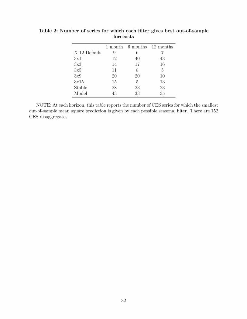
Table 2: Number of series for which each filter gives best out-of-sampleforecasts

1 month 6 months 12 monthsX-12-Default 9 6 73x1 12 40 433x3 14 17 163x5 11 8 53x9 20 20 103x15 15 5 13Stable 28 23 23Model 43 33 35

NOTE: At each horizon, this table reports the number of CES series for which the smallestout-of-sample mean square prediction is given by each possible seasonal filter. There are 152CES disaggregates.

32

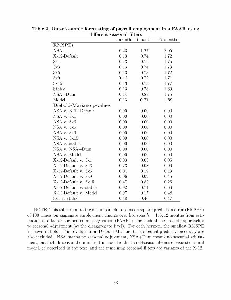
Table 3: Out-of-sample forecasting of payroll employment in a FAAR usingdifferent seasonal filters

1 month 6 months 12 monthsRMSPEsNSA 0.23 1.27 2.05X-12-Default 0.13 0.74 1.723x1 0.13 0.75 1.753x3 0.13 0.74 1.733x5 0.13 0.73 1.723x9 0.12 0.72 1.713x15 0.13 0.73 1.77Stable 0.13 0.73 1.69NSA+Dum 0.14 0.83 1.75Model 0.13 0.71 1.69Diebold-Mariano p-valuesNSA v. X-12 Default 0.00 0.00 0.00NSA v. 3x1 0.00 0.00 0.00NSA v. 3x3 0.00 0.00 0.00NSA v. 3x5 0.00 0.00 0.00NSA v. 3x9 0.00 0.00 0.00NSA v. 3x15 0.00 0.00 0.00NSA v. stable 0.00 0.00 0.00NSA v. NSA+Dum 0.00 0.00 0.00NSA v. Model 0.00 0.00 0.00X-12-Default v. 3x1 0.03 0.03 0.05X-12-Default v. 3x3 0.73 0.08 0.06X-12-Default v. 3x5 0.04 0.19 0.43X-12-Default v. 3x9 0.06 0.09 0.45X-12-Default v. 3x15 0.47 0.82 0.25X-12-Default v. stable 0.92 0.74 0.66X-12-Default v. Model 0.97 0.17 0.483x1 v. stable 0.48 0.46 0.47

NOTE: This table reports the out-of-sample root mean square prediction error (RMSPE)of 100 times log aggregate employment change over horizons h = 1, 6, 12 months from esti-mation of a factor augmented autoregression (FAAR) using each of the possible approachesto seasonal adjustment (at the disaggregate level). For each horizon, the smallest RMSPEis shown in bold. The p-values from Diebold-Mariano tests of equal predictive accuracy arealso included. NSA means no seasonal adjustment, NSA+Dum means no seasonal adjust-ment, but include seasonal dummies, the model is the trend+seasonal+noise basic structuralmodel, as described in the text, and the remaining seasonal filters are variants of the X-12.

33

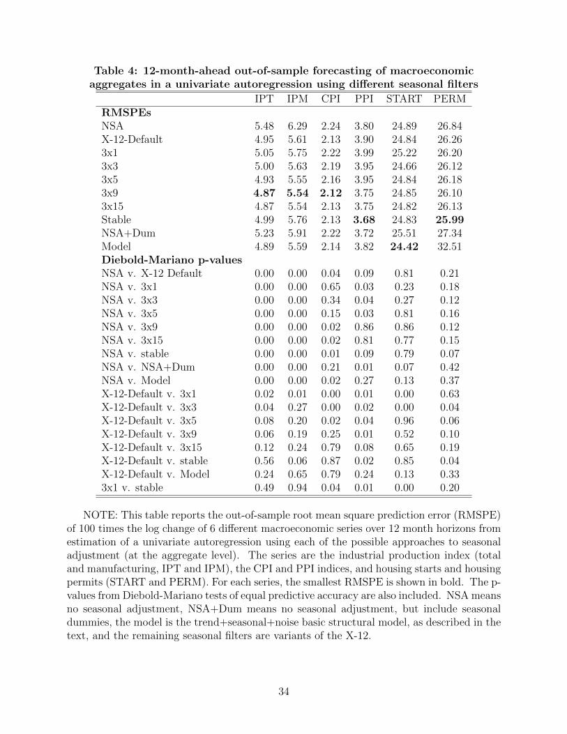
Table 4: 12-month-ahead out-of-sample forecasting of macroeconomicaggregates in a univariate autoregression using different seasonal filters

IPT IPM CPI PPI START PERMRMSPEsNSA 5.48 6.29 2.24 3.80 24.89 26.84X-12-Default 4.95 5.61 2.13 3.90 24.84 26.263x1 5.05 5.75 2.22 3.99 25.22 26.203x3 5.00 5.63 2.19 3.95 24.66 26.123x5 4.93 5.55 2.16 3.95 24.84 26.183x9 4.87 5.54 2.12 3.75 24.85 26.103x15 4.87 5.54 2.13 3.75 24.82 26.13Stable 4.99 5.76 2.13 3.68 24.83 25.99NSA+Dum 5.23 5.91 2.22 3.72 25.51 27.34Model 4.89 5.59 2.14 3.82 24.42 32.51Diebold-Mariano p-valuesNSA v. X-12 Default 0.00 0.00 0.04 0.09 0.81 0.21NSA v. 3x1 0.00 0.00 0.65 0.03 0.23 0.18NSA v. 3x3 0.00 0.00 0.34 0.04 0.27 0.12NSA v. 3x5 0.00 0.00 0.15 0.03 0.81 0.16NSA v. 3x9 0.00 0.00 0.02 0.86 0.86 0.12NSA v. 3x15 0.00 0.00 0.02 0.81 0.77 0.15NSA v. stable 0.00 0.00 0.01 0.09 0.79 0.07NSA v. NSA+Dum 0.00 0.00 0.21 0.01 0.07 0.42NSA v. Model 0.00 0.00 0.02 0.27 0.13 0.37X-12-Default v. 3x1 0.02 0.01 0.00 0.01 0.00 0.63X-12-Default v. 3x3 0.04 0.27 0.00 0.02 0.00 0.04X-12-Default v. 3x5 0.08 0.20 0.02 0.04 0.96 0.06X-12-Default v. 3x9 0.06 0.19 0.25 0.01 0.52 0.10X-12-Default v. 3x15 0.12 0.24 0.79 0.08 0.65 0.19X-12-Default v. stable 0.56 0.06 0.87 0.02 0.85 0.04X-12-Default v. Model 0.24 0.65 0.79 0.24 0.13 0.333x1 v. stable 0.49 0.94 0.04 0.01 0.00 0.20

NOTE: This table reports the out-of-sample root mean square prediction error (RMSPE)of 100 times the log change of 6 different macroeconomic series over 12 month horizons fromestimation of a univariate autoregression using each of the possible approaches to seasonaladjustment (at the aggregate level). The series are the industrial production index (totaland manufacturing, IPT and IPM), the CPI and PPI indices, and housing starts and housingpermits (START and PERM). For each series, the smallest RMSPE is shown in bold. The p-values from Diebold-Mariano tests of equal predictive accuracy are also included. NSA meansno seasonal adjustment, NSA+Dum means no seasonal adjustment, but include seasonaldummies, the model is the trend+seasonal+noise basic structural model, as described in thetext, and the remaining seasonal filters are variants of the X-12.

34

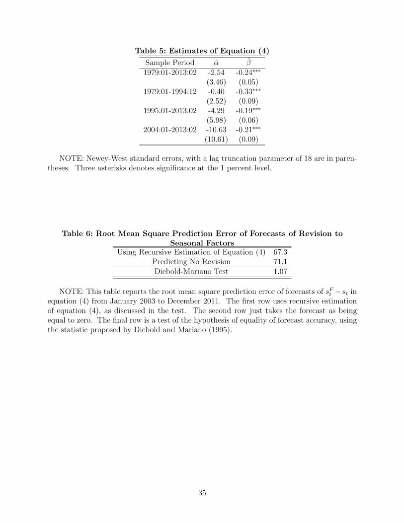
Table 5: Estimates of Equation (4)

Sample Period α β1979:01-2013:02 -2.54 -0.24∗∗∗

(3.46) (0.05)1979:01-1994:12 -0.40 -0.33∗∗∗

(2.52) (0.09)1995:01-2013:02 -4.29 -0.19∗∗∗

(5.98) (0.06)2004:01-2013:02 -10.63 -0.21∗∗∗

(10.61) (0.09)

NOTE: Newey-West standard errors, with a lag truncation parameter of 18 are in paren-theses. Three asterisks denotes significance at the 1 percent level.

Table 6: Root Mean Square Prediction Error of Forecasts of Revision toSeasonal Factors

Using Recursive Estimation of Equation (4) 67.3Predicting No Revision 71.1Diebold-Mariano Test 1.07

NOTE: This table reports the root mean square prediction error of forecasts of sFt − st inequation (4) from January 2003 to December 2011. The first row uses recursive estimationof equation (4), as discussed in the test. The second row just takes the forecast as beingequal to zero. The final row is a test of the hypothesis of equality of forecast accuracy, usingthe statistic proposed by Diebold and Mariano (1995).

35

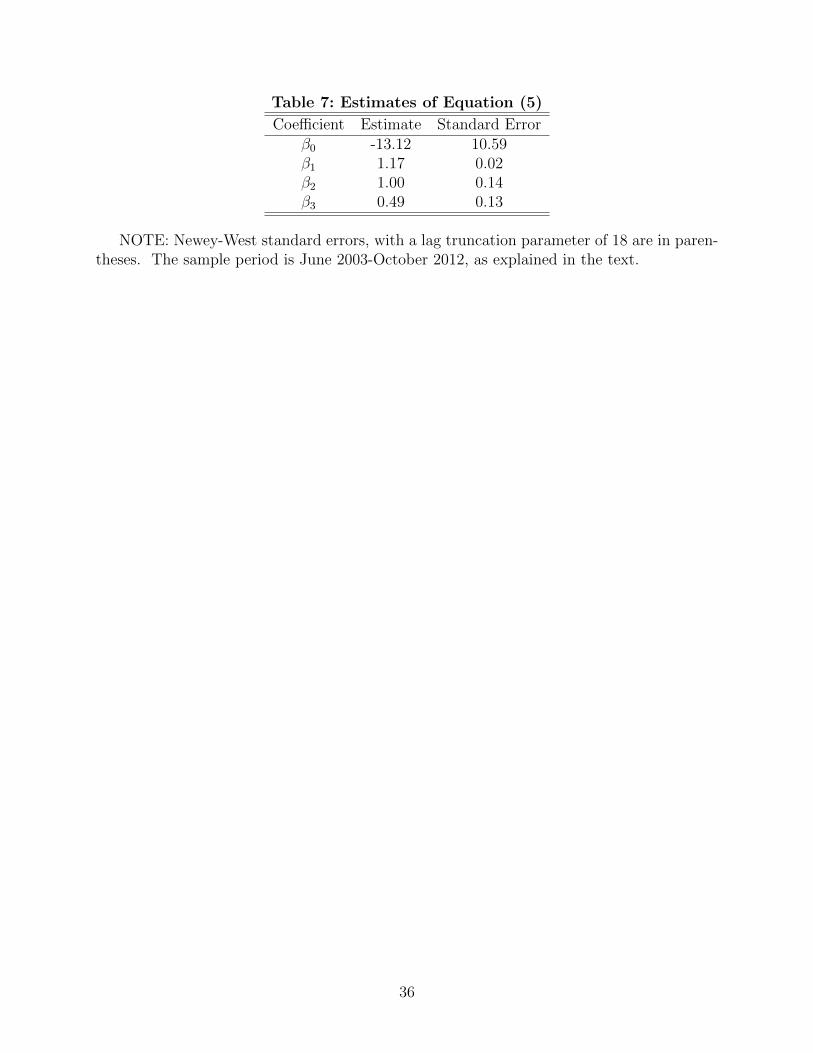
Table 7: Estimates of Equation (5)

Coefficient Estimate Standard Errorβ0 -13.12 10.59β1 1.17 0.02β2 1.00 0.14β3 0.49 0.13

NOTE: Newey-West standard errors, with a lag truncation parameter of 18 are in paren-theses. The sample period is June 2003-October 2012, as explained in the text.

36

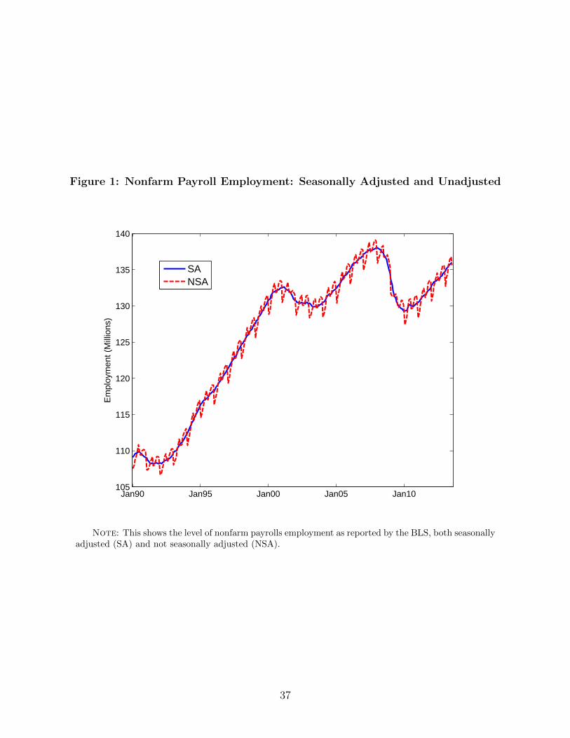
Figure 1: Nonfarm Payroll Employment: Seasonally Adjusted and Unadjusted

Jan90 Jan95 Jan00 Jan05 Jan10105

110

115

120

125

130

135

140

Em

ploy

men

t (M

illio

ns)

SANSA

Note: This shows the level of nonfarm payrolls employment as reported by the BLS, both seasonallyadjusted (SA) and not seasonally adjusted (NSA).

37

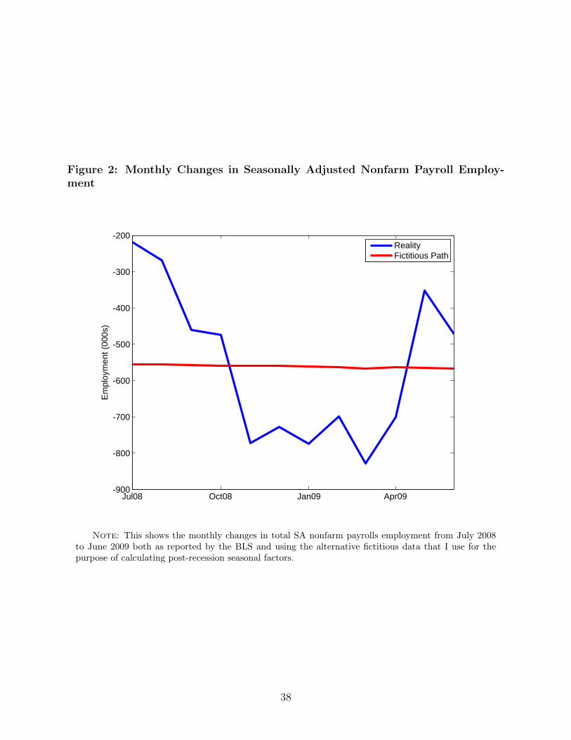
Figure 2: Monthly Changes in Seasonally Adjusted Nonfarm Payroll Employ-ment

Jul08 Oct08 Jan09 Apr09-900

-800

-700

-600

-500

-400

-300

-200

Em

ploy

men

t (0

00s)

RealityFictitious Path

Note: This shows the monthly changes in total SA nonfarm payrolls employment from July 2008to June 2009 both as reported by the BLS and using the alternative fictitious data that I use for thepurpose of calculating post-recession seasonal factors.

38

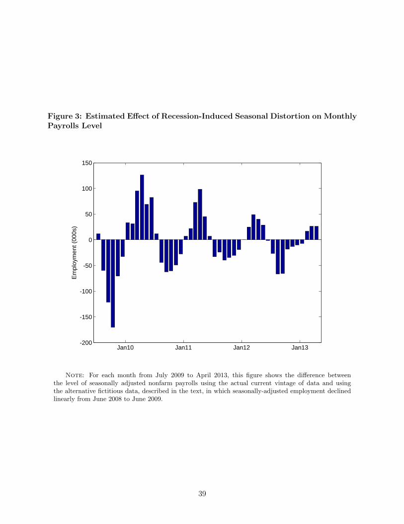
Figure 3: Estimated Effect of Recession-Induced Seasonal Distortion on MonthlyPayrolls Level

Jan10 Jan11 Jan12 Jan13-200

-150

-100

-50

0

50

100

150

Em

ploy

men

t (0

00s)

Note: For each month from July 2009 to April 2013, this figure shows the difference betweenthe level of seasonally adjusted nonfarm payrolls using the actual current vintage of data and usingthe alternative fictitious data, described in the text, in which seasonally-adjusted employment declinedlinearly from June 2008 to June 2009.

39

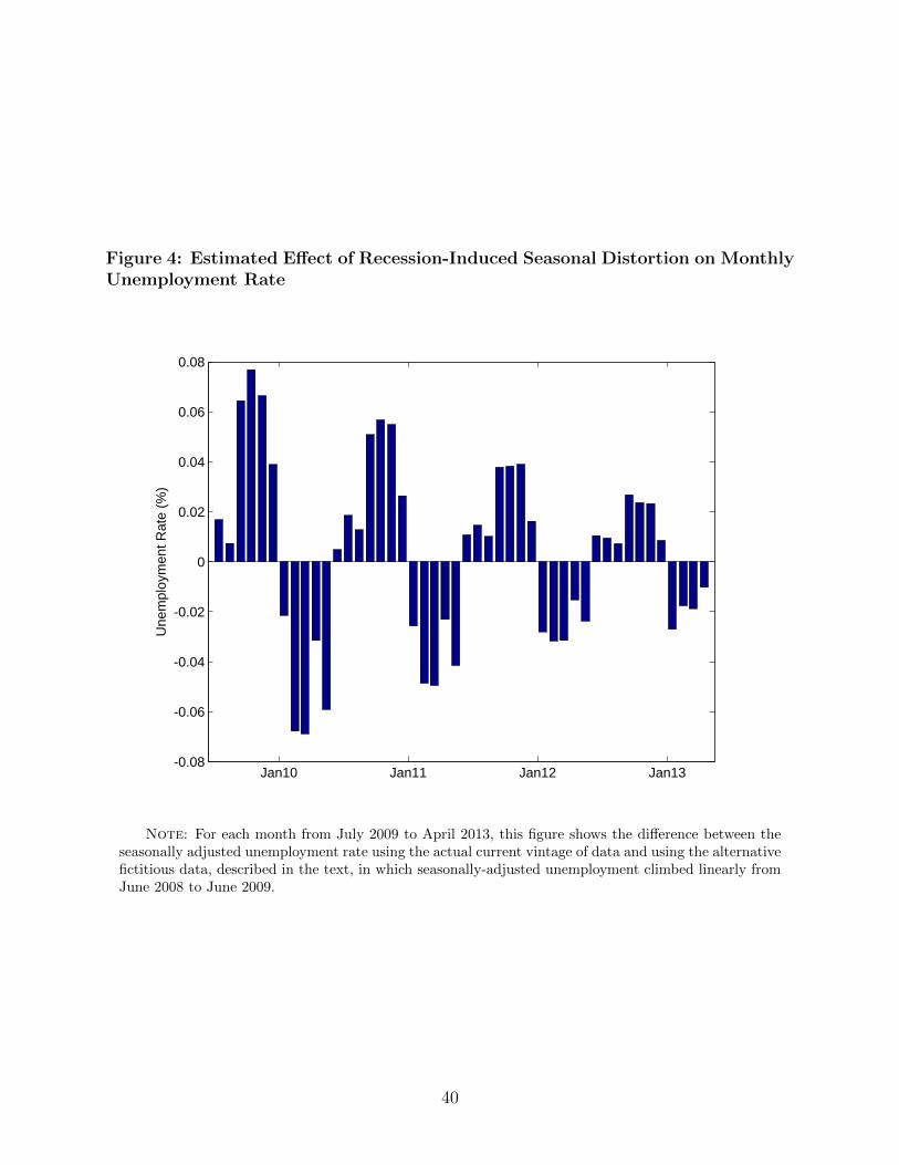
Figure 4: Estimated Effect of Recession-Induced Seasonal Distortion on MonthlyUnemployment Rate

Jan10 Jan11 Jan12 Jan13-0.08

-0.06

-0.04

-0.02

0

0.02

0.04

0.06

0.08

Une

mpl

oym

ent

Rat

e (%

)

Note: For each month from July 2009 to April 2013, this figure shows the difference between theseasonally adjusted unemployment rate using the actual current vintage of data and using the alternativefictitious data, described in the text, in which seasonally-adjusted unemployment climbed linearly fromJune 2008 to June 2009.

40

Figure 5: Estimated Effect of Recession-Induced Seasonal Distortion on MonthlyPayrolls Level: Alternative Methodology

Jan10 Jan11 Jan12 Jan13-100

-50

0

50

100

150

Em

ploy

men

t (0

00s)

Note: For each month from January 2010 to April 2013, this figure shows the difference betweenthe level of seasonally adjusted nonfarm payrolls using the actual current vintage of data and using thedata using the alternative seasonal adjustment in which data from 2008 and 2009 are treated as missing(with a level shift in 2010:01), following Evans and Tiller (2013).

41

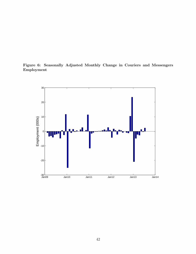
Figure 6: Seasonally Adjusted Monthly Change in Couriers and MessengersEmployment

Jan09 Jan10 Jan11 Jan12 Jan13 Jan14-30

-20

-10

0

10

20

30

Em

ploy

men

t (0

00s)

42

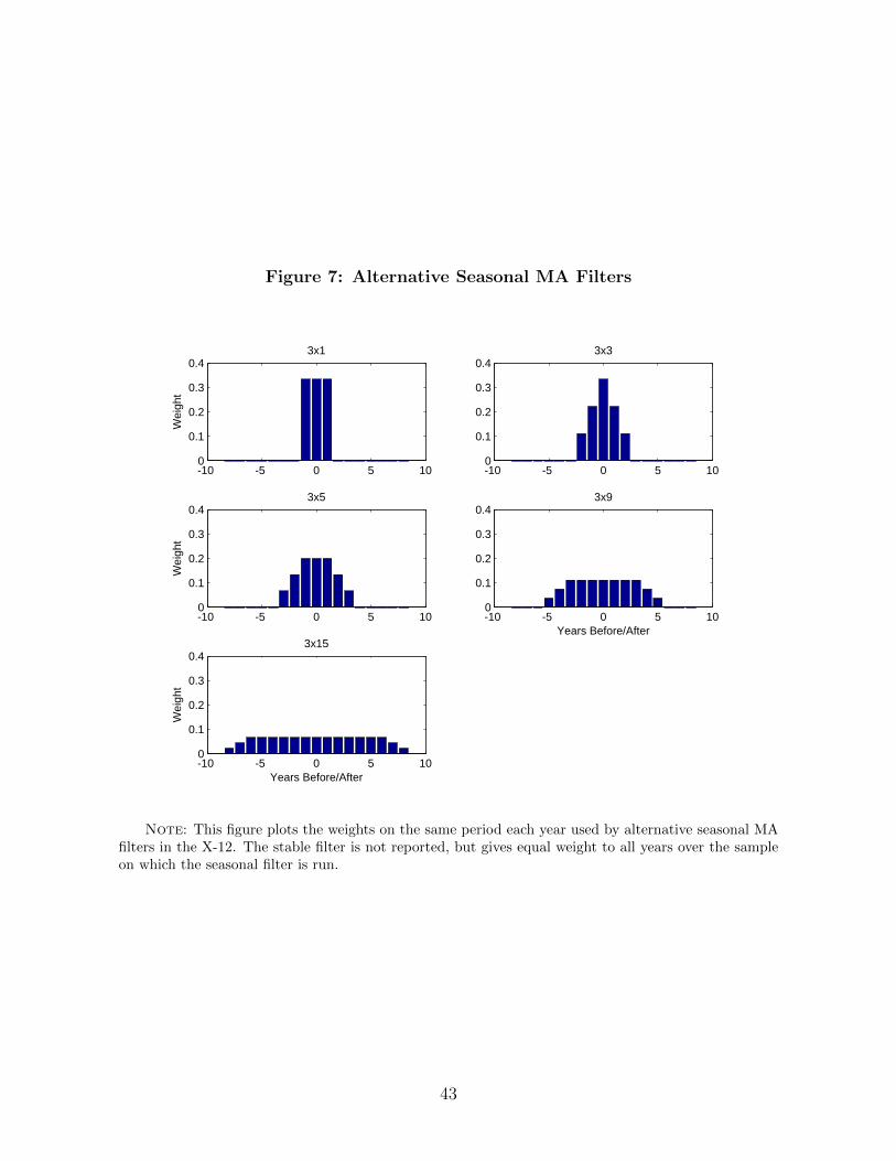
Figure 7: Alternative Seasonal MA Filters

-10 -5 0 5 100

0.1

0.2

0.3

0.43x1

Wei

ght

-10 -5 0 5 100

0.1

0.2

0.3

0.43x3

-10 -5 0 5 100

0.1

0.2

0.3

0.43x5

Wei

ght

-10 -5 0 5 100

0.1

0.2

0.3

0.43x9

Years Before/After

-10 -5 0 5 100

0.1

0.2

0.3

0.43x15

Wei

ght

Years Before/After

Note: This figure plots the weights on the same period each year used by alternative seasonal MAfilters in the X-12. The stable filter is not reported, but gives equal weight to all years over the sampleon which the seasonal filter is run.

43

Figure 8: Estimated Effect of Shock to Employment

Jan05 Jul07 Jan10 Jul12-0.2

0

0.2

0.4

0.6

0.8

1

1.2

Em

ploy

men

t (P

erce

nt)

Note: This figure plots the effect on SA aggregate employment resulting from a hypothetical 1percent increase in NSA disaggregate employment in January-March 2005.

44

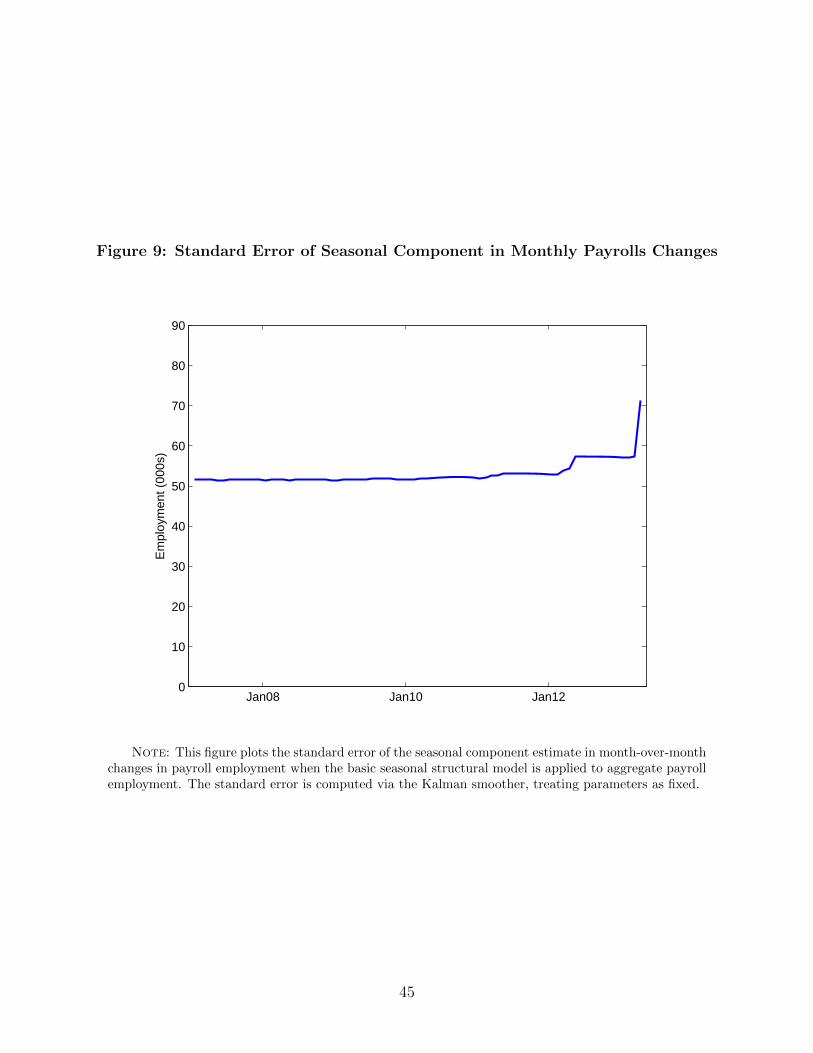
Figure 9: Standard Error of Seasonal Component in Monthly Payrolls Changes

Jan08 Jan10 Jan120

10

20

30

40

50

60

70

80

90

Em

ploy

men

t (0

00s)

Note: This figure plots the standard error of the seasonal component estimate in month-over-monthchanges in payroll employment when the basic seasonal structural model is applied to aggregate payrollemployment. The standard error is computed via the Kalman smoother, treating parameters as fixed.

45

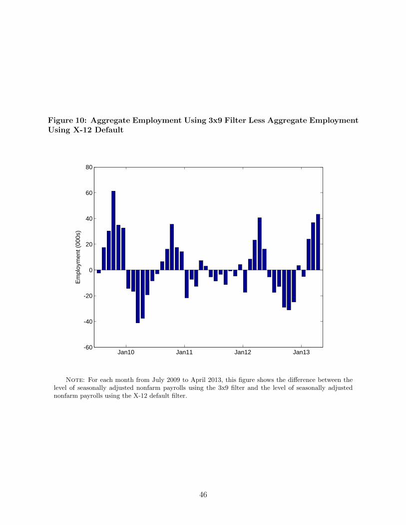
Figure 10: Aggregate Employment Using 3x9 Filter Less Aggregate EmploymentUsing X-12 Default

Jan10 Jan11 Jan12 Jan13-60

-40

-20

0

20

40

60

80

Em

ploy

men

t (0

00s)

Note: For each month from July 2009 to April 2013, this figure shows the difference between thelevel of seasonally adjusted nonfarm payrolls using the 3x9 filter and the level of seasonally adjustednonfarm payrolls using the X-12 default filter.

46

Appendix: Description of the X-12 ARIMA Algorithm

This appendix describes the X-12 adjustment process using the default settings, as it appliesto monthly data. Let yt be the monthly time series that is to be seasonally adjusted. Theidea of the X-12 algorithm is to estimate a decomposition of the series into trend, seasonaland irregular components. The decomposition could be multiplicative or additive, at theuser’s discretion. Multiplicative means that the series is the product of trend, seasonal andirregular components; additive means that it is their sum. There are two further options inX-12: log-additive and pseudo-additive, but I omit these. Before beginning, the raw datamay be adjusted for special effects (in the context of the CES, this include strikes or thebuildup in federal employment around the decennial census). The algorithm then involvesthe following iterations:

First on iteration A, the time series is specified to be of a seasonal ARIMA form, suchthat:

φ(L)Φ(L12)(1− L)d(1− L12)D(yt − β′xt) = θ(L)Θ(L12)εt

where xt are user-chosen regressors, L denotes the lag operator, φ(L), Φ(L12), θ(L) andΘ(L12) are polynomials of orders p, P , q and Q respectively, d and D are integer differenceoperators and εt is an iid error term. Regressors for Easter, Labor Day and Thanksgivingare built in. In the context of the CES, a regressor for the number of weeks since the lastsurvey (always 4 or 5) for each month except March is also included. March is excluded,because the number of weeks since last survey will be 4 (except for once every seven leapyears). Regressors that capture outliers, level shifts, or “ramps” (as employed by Kropf andHudson (2012)) may also be included. The model is then estimated by maximum likelihoodand used to generate forecasts of future values of yt, and backcasts. In this step yt may bereplaced by a nonlinear transformation, such as the log. If β denotes the estimator of β,then the data are replaced by yt − β′xt.

The next iteration, iteration B, involves the following steps:

(1) An initial estimate of the trend is computed as

T(1)t =

1

24yt−6 +

1

12yt−5...+

1

12yt+5 +

1

24yt+6

(2) An initial detrended series is computed as y(1)t = yt/T

(1)t for a multiplicative decompo-

sition or y(1)t = yt − T (1)

t for an additive decomposition.

(3) Compute an initial preliminary seasonal factor from the 3x3 seasonal filter:

S(1,P )t =

1

9y(1)t−24 +

2

9y(1)t−12 +

3

9y(1)t +

2

9y(1)t+12 +

1

9y(1)t+24

(4) Compute an initial seasonal factor as:

S(1)t =

S(1,P )t

124S(1,P )t−6 + 1

12S(1,P )t−5 ...+ 1

12S(1,P )t+5 + 1

24S(1,P )t+6

47

for a multiplicative decomposition, or

S(1)t = S

(1,P )t − { 1

24S(1,P )t−6 +

1

12S(1,P )t−5 ...+

1

12S(1,P )t+5 +

1

24S(1,P )t+6 }

for an additive decomposition. This ensures that the seasonal factors approximatelyaverage to one over the course of the year.

(5) Compute the initial seasonally adjusted data as ySA(1)t = yt/S

(1)t for a multiplicative

decomposition of ySA(1)t = yt − S(1)

t for an additive decomposition.

(6) Compute a new estimate of the trend from the Henderson filter:

T(2)t = ΣH

j=−HhjySA(1)t+j

where

hj =315{(H + 1)2 − j2}{(H + 2)2 − j2}{(H + 3)2 − j2}{3(H + 2)2 − 16− 11j2}

8{H + 2}{(H + 2)2 − 1}{4(H + 2)2 − 9}{4(H + 2)2 − 25},

and H is chosen from 4 or 6 (giving a 9 or 13-term filters) based on the ratio of theabsolute value of the irregular component to the absolute value of the trend (the I/Cratio), as decomposed above. If this ratio is smaller than 1, then set H = 4, otherwiseH = 6.

(7) A new detrended series is computed as y(2)t = yt/T

(2)t for a multiplicative decomposition

or y(2)t = yt − T (2)

t for an additive decomposition.

(8) Compute a preliminary seasonal factor from the 3x5 seasonal filter:

S(2,P )t =

1

15y(2)t−36 +

2

15y(2)t−24 +

3

15y(2)t−12 +

3

15y(2)t +

3

15y(2)t+12 +

2

15y(2)t+24 +

1

15y(2)t+36

(9) Compute a final seasonal factor, S(2)t as in step 5, and then the finally seasonally

adjusted data, ySA(2)t , as in step 4.

(10) Compute a final estimate of the trend as

T(3)t = ΣH

j=−HhjySA(2)t+j

where hj is determined as in step 6.

(11) Compute the irregular component, I(3)t of the series as

ySA(2)t

T(3)t

or ySA(2)t − T (3)

t for mul-

tiplicative and additive decompositions, respectively.

48

(12) Next I turn to the “trading day” adjustment. Let Djt be the number of days of day-of-the week j in month t (j is indexed from 1 to 7). Let Nt denote the number of daysin month t and N be the average number of days per month.

For the multiplicative decomposition, estimate the equation:

NI(3)t −Nt = Σ6

j=1βj(Djt −D7t) + et

by OLS, letting βj denote the estimate of βj. Then divide the irregular component by:

1

N[Σ6

j=1βj(Djt −D7t) + Σ7j=1βj]

For the additive decomposition, instead estimate the equation:

I(3)t = β0(Nt − N) + Σ6

j=1βj(Djt −D7t) + et

again by OLS and subtract Σ6j=1βj(Djt −D7t) from the irregular component.

(13) Compute a 60 month rolling standard deviation of the irregular component, σ(1)t . Re-

compute this 60 month rolling standard deviation of the irregular component droppingany observations for which |I(3)t | > 2.5σ

(1)t . Call this rolling standard deviation σ

(2)t .

Define the weighting function

wt = min(max(0, 2.5− |I(3)t |σ(2)t

), 1)

If wt < 1, replace I(3)t with the average value for that month over the 60 month win-

dow weighting the month in the current year by wt and the same month in other yearsby 1(wt = 1). The data are then replaced with the sum/product of the trend, sea-sonal and irregular components, as currently computed, in the additive/multiplicativedecompositions, respectively.

The next iteration, the C iteration, involves repeating steps 1-13 again. However, on theC iteration, in step 6, H = 4 if the I/C ratio is below 1, H = 6 if the I/C ratio is between 1and 3.5, and otherwise, H = 11.

On the final iteration, the D iteration, the series are run through steps 1-9 one last time.However, on the D iteration, step 6 is modified as in the C iteration. Also, the filter chosenin step 8 will be the 3x3, 3x5 or 3x9 depending on the value of the I/S ratio, which is theratio of the absolute value of the irregular component to the absolute value of the seasonalcomponent. If this ratio is below 2.5, the 3x3 filter is used. If it is between 3.5 and 5.5,the 3x5 filter is used. If it is above 6.5, the 3x9 filter is used. If it does not fall into any ofthese three regions, then the last year of data is deleted and the procedure is re-run. Thisalgorithm is iterated until one of the three filters is selected or five years’ data have beendropped, whichever comes sooner. If in the end, no filter has been selected, the 3x5 filter is

49

employed. Instead of the default setting described here, the seasonal moving average filterin the X-12 process can be fixed at the 3x1, 3x3, 3x5, 3x9, 3x15 or stable alternatives, asconsidered in section 3 of the paper.

In the A iteration, the user decides how far to extend the series forward and backwards.Depending on this choice, there may not be enough data for the seasonal filters in steps 3and 8 of the B, C and D iterations to be applied at the start and end of the sample. Inthis case, the filters are replaced with asymmetric filters which are provided on page 45 ofLadiray and Quenneville (1989). For example, the asymmetric 3x3 filter with no future dataavailable puts weights of 11/27 on the current and previous year and a weight of 5/27 onthe second previous year. The estimates of the trend in steps 1 and 6 likewise need to beadjusted, as also discussed in that book. The CES implementation of the X-12 ARIMAseasonal adjustment process does no backcasting, and allows forecasts to extend the seriesby only 24 months. Thus asymmetric filters will apply at the start and end of the sample.

The final seasonally adjusted data consist of the original data divided by/less the seasonalfactor in the multiplicative/additive model, respectively.

50