unordered and ordered sample from dirichlet distribution · (1 - v1)v2. iterating, the final sbp of...

Ann, Inst. Statist. Math. Vol. 57, No. 3, 597-616 (2005) @2005 The Institute of Statistical Mathematics

UNORDERED AND ORDERED SAMPLE FROM DIRICHLET DISTRIBUTION

THIERRY HUILLET

Laboratoire de Physique Thdorique et Moddlisation, CNRS-UMR 8089 et Universitd de Cergy-Pontoise, 5 mail Gay-Lussac, 95031, Neuville sur Oise, France,

e-mail: [email protected]

(Received March 2, 2004; revised September 1, 2004)

Abstract . Consider the random Dirichlet partition of the interval into n fragments with parameter 0 > 0. Explicit results on the statistical structure of its size-biased permutation are recalled, leading to (unordered) Ewens and (ordered) Donnelly-Tavar~-Griffiths sampling formulae from finite Dirichlet partitions. We use these preliminary statistical results on frequencies distribution to address the following sampling problem: what are the intervals between new sampled categories when sampling is from Dirichlet populations? The results obtained are in accordance with the ones found in sampling theory from random proportions with GEM(3,) distribution. These can be obtained from Dirichlet model when considering the Kingman limit n T co, 0 & 0 while nO = ~ > O.

Key words and phrases: Random discrete distribution, Dirichlet partition, size- biased permutation, GEM, Ewens and Donnelly-Tavar~-Griffiths sampling formulae, intervals between new sampled species.

1. Introduction

The joint distribution of unordered (or ordered) frequencies of a sample from random proportions with Griffiths-Engen-McCloskey, or GEM(~ / ) , distribution is the Donnelly- Tavar6-Griffiths formula (or the Ewens sampling formulae). The G E M ( ~ / ) distribution will be defined later (see also Kingman (1993), Chapter 9, for example).

We first reconsider the same sampling problems and formulae when sampling is from random proportions with Dirichlet Dn(O) distribution, hence with a finite number n of fragments in the partition. The usual Ewens and Donnelly-Tavar6-Griffiths sampling formulae can be found when passing to the Kingman limit n T oc, 0 ~ 0, nO = ~ /> O. These preliminary results which are recalled are used to study the intervals between consecutive categories and number of distinct categories when sampling is from Dn(O). The results obtained are in accordance with particular cases of those of Yamato-Sibuya- Nomachi when sampling is from G E M ( " / ) , while passing to the Kingman limit.

The organization of this manuscript is the following. Consider the random Dirichlet partition of the interval into n fragments with parameter 0 > 0. Elementary properties of its D~(O) distribution are first recalled in Section 2. Explicit results on the law of its size-biased permutation are also recalled there. These are useful when considering the Donnelly-Tavar~-Griffiths sampling formula from Dirichlet partitions in subsequent Subsection 3.3, as given in Theorem 3.3. A size-biased permutation of the fragments

597

598 THIERRY HUILLET

sizes is the one obtained in a size-biased sampling process without replacement from a Dirichlet partition. The main points which we recall are the following: in Lemma 2.1, its residual allocation model structure is recalled. In Lemma 2.2, the order in which the consecutive fragments are visited is considered. In Theorem 2.1, we recall the joint law of the size-biased permutation fragments sizes explicitly. Using this, it is recalled in Corollary 2.1 that consecutive fragments in the size-biased permuted partition are arranged in stochastic descending order.

Section 3 recalls the (unordered) Ewens and (ordered) Donnelly-Tavar~-Griffiths sampling formulae when sampling is from finite Dirichlet partitions. In more details, Subsection 3.1 is devoted to the first Ewens sampling formula when sampling is from Dirichlet partition Dn(O). Here the order in which sequentially sampled species arise is irrelevant. Subsection 3.2 concerns the second Ewens sampling formula under the same hypothesis (as a problem of random partitioning of the integers) and Subsection 3.3 deals with the finite Dirichlet version of the Donnelly-Tavar~-Griffiths sampling formula. Here, the order of appearance of sampled species is taken into account. Main results are displayed in Theorems 3.1, 3.2 and 3.3 for each of the problems alluded to. As corollaries to these theorems, the usual well-known sampling formulae can be deduced in each case when sampling is from GEM distribution which is the limiting version of the size-biased permutation of Dirichlet partitions in the sense of Kingman.

The main body of our new sampling results is in Section 4. We use the previous statistical results on frequencies distribution to address the following sampling problem: what are the intervals between new sampled categories until exhaustion of the list, when sampling is from Dirichlet populations? One intuitively expects these intervals to be increasing while approaching complete exhaustion. Our main results on the statistical structure of these intervals are summarized in Theorems 4.1, 4.2 and 4.3, considering both cases of a fixed and then unlimited sample size.

The results obtained are in accordance with the Yamato-Sibuya-Nomachi ones when sampling is from random proportions with GEM(v) distribution. These can naturally be obtained from Dirichlet model when considering the Kingman limit. Results in this direction are displayed in Corollaries 4.1, 4.2 and 4.3 to Theorems 4.1, 4.2 and 4.3, respectively.

2. Size-biased permutation of the Dirichlet distribution

2.1 Dirichlet partition of the interval Consider the following random partition into n fragments of the unit interval. Let

0 > 0 be some parameter and assume that the random fragments' sizes Sn := ($1 , . . . , Sn) (with ~-~=1 S m = 1) is distributed according to the (exchangeable) Dirichlet D,~(O) density function on the simplex, that is to say

r(n0)r(0) n fl 0 - i (2.1) / s l ..... Sn(81 , . . . ,Sn) - 8~--1)" m=l

Alternatively, the law of Sn := ($1, �9 �9 S~) is characterized by its joint moment function

( 2 . 2 ) E = =1 -~- Era----1 qm') F(0)

We shall put Sn d Dn(O) if S~ is Dirichlet distributed with parameter 0.

SAMPLE FROM DIRICHLET PARTITION 599

If this is so, Sm d Sn, m = 1 , . . . , n, independently of m and the individual fragments sizes are all identically distributed. Their common density on the interval (0, 1) is a beta(0, (n - 1)0) density.

When 8 -- 1, the partition model equations (2.1), (2.2) corresponds to the standard uniform partition model of the interval.

In the random division of the interval as in equation (2.1), although all fragments are identically distributed with sizes of order n-1, the smallest fragment's size grows like n -(~176 while the one of the largest is of order I log(n log ~ n). The smaller O is, the larger (smaller) the largest (smallest) fragments' size is: hence, the smaller O is, the more the values of the Sms are, with high probability, disparate. Smaller the parameter, the size of the largest fragment S(1) tends to dominate the other ones. On the contrary, large values of O correspond to situations in which the range of fragments' sizes is lower: the fragments' sizes look more homogeneous and distribution equation (2.1) concentrates on its centre. For large O, the diversity of the partition is small.

Although Sn has a degenerate weak limit when n T oc, O l 0 while nO = V > 0, this situation is worth being considered (as first noted by Kingman (1975)). Indeed, many interesting statistical features emerge.

2.2 Size-biased permutation of Dirichlet partitions The results on size-biased permutation of Dirichlet distributions presented in this

section are not new. When O = 1, they can be found in Huillet (2003); they were generalized to all O > 0 in Barrera et al. (2005), to solve a problem consisting in computing the search-cost distribution arising from heaps processes. Part of them are reproduced here for the sake of completeness and to make the presentation self-contained. They will prove useful in the sequel.

Assume some observer is sampling the unit interval as follows: drop points at random onto this randomly broken interval and record the corresponding numbers of visited fragments. We shall consider the problem of determining the order in which the various fragments are discovered in such a sampling process. To avoid revisiting the same fragment many times, once it has been discovered, we need to remove it from the population as soon as it has been met in the sampling process. But to do that, the law of its size is needed. Once this is done, after renormalizing the remaining fragments' sizes, we are left with a population of n - 1 fragments, the sampling of which will necessarily supply a so far undiscovered fragment. The distribution of its size can itself be computed and so forth, renormalizing again, until the whole available fragments population has been visited. In this way, not only the visiting order of the different fragments can be un- derstood but also their sizes. The purpose of this section is to describe the statistical structure of the size-biased permutation of the fragments' sizes as those obtained while avoiding the ones previously encountered in a sampling process from Dirichlet partition.

�9 The R A M structure of size-biased permutation. Let S n := ( S I , . . . , Sn) be the random partition of the interval [0, 1] considered here. Let L1 be the length of the first randomly chosen fragment M1 := M, so with L1 := SM1 and P(M1 = m l I ~n) = Sin1.

One may check that L1 d beta(1 + O, (n - 1)8). A standard problem is to iterate the size-biased picking procedure, by avoiding the fragments already encountered: by doing so, a size-biased permutation (SBP) of the fragments is obtained. It turns out that SBP(Sn) has a residual allocation model (RAM) structure.

6 0 0 T H I E R R Y H U I L L E T

In the first step of this size-biased picking procedure indeed, Sn =: S (~ --~ S( 1 ) (L1,SI,..�9149149149 which may be written as Sn --~ (L1, ( 1 - L1) n- lJ ,

with S(1) 1 := (5'~1),�9 ~(1) ~(1) S (1)) a new random partition of the unit �9 " ' ~ M 1 - - 1 ' ~ M 1 + 1 ' " " " '

interval into n - 1 random fragments�9

Given L1 d beta(1 + 0, (n - 1)0), the conditional joint distribution of the remaining

components of Sn is the same as that of (1 - ~,l)On_ l r ~dl) where the (n - 1) -vec tor 8(1_) 1 a Dn-l(0) has the distribution of a Dirichlet random partition into n - 1 fragments (see

Kingman (1993), Chapter 9). Furthermore, S(1_)1 is independent of 1 - L1. Pick next at

random an interval in S(~_)I and call V2 its length, now with distribution beta(1 + 0, ( n - 2)0), and iterate until all fragments have been exhausted.

With V1 := L1, the length of the second fragment by avoiding the first reads L2 -- (1 - V1)V2. Iterating, the final SBP of Sn is Ln := ( L I , . . . , L n ) and we shall put Ln = SBP(S , ) . From this construction, we easily get

LEMMA 2�9149 Let E~ = SBP( S~). I f (V1, . . . , Vn-1) is an independent sample with

distribution Vk a beta(1 + 0, (n - k)O), k = 1 , . . . , n - 1, then,

k--1

(2�9 Lk = H ( 1 -- Vi)Vk, k = 1 , . . . , n - 1 i----1

n - - 1 n - - 1

(2�9 L n = I - E L k = H ( 1 - V i ) k = l k = l

is the R A M representation of the size-biased permutation Ln of Sn.

Note that Vi := 1 - V~ a be ta( (n- i )O, 1 +0) and that V~ should be set to 1. These are well-known construction and properties; see Kingman ((1993), Chapter 9, Section 6) and Donnelly (1986, 1991).

This RAM representation allows to compute the joint distribution of the size- biased permutation L~ of Sn. We shall say in the sequel that, if Ln = SBP(S~), then

Ln a SBDn(O) assuming that Sn d Dn(O). Before addressing this problem, we shall first consider the order in which fragments are visited�9

�9 The visiting order of the fragments in the SBP process. For any permutation {ml, mn} of {1, , n}, with M~ M' k = 1,. n, the first k distinct fragments �9 . �9 . �9149 , �9149149 ~, �9149

numbers which have been visited in the SBP sampling process, we have

k - - 1

, Sm~ Smk, P ( M ~ = m ~ , � 9 1 4 9 i=IH 1 _ E~=lSm ' (2.5)

so that

(2.6)

As a result,

(2�9

~k P ( M ~ = m } I S~,Ms = ml,.�9149 1 ~- mk-1) = l _ E / k i 1 Sml�9

P(M~ = m I S~) = Sm k - 1

S r n ~

E H 1 -- ~-~'.~:, Sin, (mlg!...y~mk_i)9~ i=l


is the conditional (given Sn) probability that the k-th visited fragment is fragment number m from Dn(O).

LEMMA 2.2. Given M~ -- m l , . . . , Mk_ 1 = ink--l, Ms is uniformly distributed on the set m E { 1 , . . . , n } \ { m l # . . . # m k - 1 } . The joint probability distribution of M~, M' �9 " , k, k = 1 , . . . , n, is Bose-Einstein distribution

1 (2.8) Po(M; = m l , . .. , Ms = ink) - - k - 1 '

1-Ii=o (n - i)

with ml # . . . # m k c {1 , . . . , n}.

PROOF. Although this result is immediate by symmetry, we shall supply a short Sm~ = Sm~r

proof of it. From equation (2.6), the function Sn ---* 1-z_~t=lV'k-~ Sr~z ~--~r~r ...... k--l~ S.~

is homogeneous with degree 0. Applying (ii) of Theorem 1 p. 471 of Huillet and Martinez (2003), with {T1, . . . , Tn} iid gamma(0) distributed random variables, we get

Po(Ms = m k I MI = m l , . . . , M~_ 1 = i n k - l ) = E Ly~m#{m ~ ..... -~k-~} Sm

1 = E_EL---kTz n - k + 1

The Bose-Einstein distribution of M~,... ,/1//s results from Bayes formula. []

�9 The joint distribution of the size-biased permutation�9 The SBP of Sn is/bn with

L,~ d S B D n (0) and Sn d Dn (0). First, we have

(2.9) ( 5 1 , � 9 1 4 9 1 4 9 Ln) = (SM~,. . . , SM~),

and consequently

n-- 1 Smk Smn" (2.10) P(L1 = S i n 1 , . . . , L n = Sm~ I Sn) = H 1 - Y~=I Sm~

k=l

Consider now the joint moment function of the random size-biased permutat ion Ln = (L1, . . . , Ln). In Barrera et al. (2005), using the RAM representation of L~, the following result was proven.

THEOREM 2.1. The joint moment funct ion of the S B P L n SBDn(O) reads

[ ] I (2.11) E l~I L qk = E E k=l {ml#...7~mn} Lk=l 1 - E k = l Sraz

n-1 { r(1 + (n - k + 1)0)

= H L r(1 + 0)r( (n - k)O) k=l

sq~+ 1]

X

d = ( L 1 , . . . , L n )

r ( 1 + 0 + q k ) r ( ( n - k)O + qk+l -4-... -4- qn) ] r(1 + ~--E-+-i~:(-qi T--- ~- q~ J "

6 0 2 T H I E R R Y H U I L L E T

�9 One-dimensional marginals. From Theorem 2.1, we get the one-dimensional law of the Lks, k = 1 , . . . , n . Furthermore, one may check that the LkS are arranged in stochastically decreasing order (denoted by _). More precisely (see Barrera et al. (2005))

COROLLARY 2.1. (i) The law of Lk, for k = 1 , . . . , n, is characterized by

(2.12) k - 1

E[Lqk] -- H E[Vq]E[Vq] i = l

k-1 r ( ( n - i )0 + q ) r ( ( n - i + 1)0 + 1)

---- H F((n / ~ ) F - - - ~ - - - - i - ~ l ~ l - T q ) i----1

F(1 + 0 + q)F(1 + (n - k + 1)0) x

r(1 + 0)r(1 + (n - k + 1)0 + q)"

(ii) Let B(~-k+l)o,1 d beta((n - k + 1)0, 1). Then,

(2.13) Lk d B(n-k+l)o,1 �9 Lk-1, k = 2 , . . . , n,

where pairs B(n-k+l)o,1 and Lk-1 are mutually independent for k = 2 , . . . , n. Off) L1 ~- . . . ~- Lk ~_ . . . ~- Ln.

The Kingman limit Consider the limit n T c~, 0 I 0 while nO = V > 0. Such an asymptotic was first

considered by Kingman (1975); we shall "star" the results (as in d ) when referring to

such an asymptotic. As noted by Kingman, 8n d Dn(O) itself has no non-degenerate limit.

d , When k = o(n), recalling Vk d beta(1 + 0, (n - k)0), we have Vk .--~ V~ d beta(l , V)

and the SBDn (0) distribution converges weakly from equations (2.3), (2.4) to a Griffiths- Engen-McCloskey or GEM('~) distribution.

Namely, (L1 , . . . ,Ln ) d ( L ~ , . . . , L ~ , . . . ) =: L* where

k - 1

(2.14). L k V i V~, k >_ 1. i ~ 1

Here (Vk* ,k > 1) are lid with common law VI* d beta(1, V ) and V~ := 1 - VI* d beta(7, 1). Note that L~ _ .. . >- L~ _ . . . , and that L* is invariant under size-biased permutation. In the Kingman limit, (S(m), m = 1 , . . . , n) converges in law to a Poisson-

Dirichlet distribution (L~k),k _> 1) d pD(V ) with L~I ) > . . . > L*(k) > """ The

size-biased permutation of ( ( k ) , k > 1) is (Lk, k > 1) d G E M ( 7 ) (see Kingman (1993), Chapter 9).

The model (2.14) generates a random countable partition of the unit interval, with many fundamental invariance properties (for a review of these results and applications to Computer Science, Combinatorial Structures, Physics, Biology . . . , see Tavar~ and


Ewens (1997) and the references therein for example; this model and related ones are also fundamental in Probability Theory; see Pi tman (1996, 1999, 2002) and Pi tman and Yor (1997).

3. Dirichlet partitions: sampling formulae for unordered and ordered sequences

Ewens' sampling formula (ESF) gives the distribution of alleles (different types of genes) in a sample with size k from the Poisson-Dirichlet process PD(v) . Alternatively, it can be described in terms of sequential sampling of animals from a countable collection of distinguishable species drawn from G E M ( v ) . It provides the probability of the partition of a sample of k selectively equivalent genes into a number of alleles as population size becomes indefinitely large. Depending on whether the order of appearance of sequentially sampled species matters or not, we are led to the first ESF for unordered sequences or to the Donnelly-Tavar~-Griffiths (DTG) sampling formula for ordered sequences. A third way to describe the sample is to record the number of species in the k-sample with exactly i representatives, i = 0 , . . . , k . When doing this while assuming the species have random frequencies following GEM(~/) distribution, we are led to a second Ewens Sampling Formula. We recall here the exact expressions of both first, second Ewens and DTG sampling formulae, when sampling is from finite Dirichlet random partitions. These sampling formulae give both ESF and DTG formulae from GEM("/) when passing to the Kingman limit (see Sibuya and Yamato (1995) for further results). Most of the results (and their proofs) presented therein can be found in Huillet (2005).

3.1 The first Ewens sampling formula for Dirichlet partitions We first consider a sampling formula from Dirichlet partitions for which the or-

der in which the consecutive fragments are being discovered in the sampling process is irrelevant.

Let Sn be the above Dirichlet random partition with parameter 0 > 0. Let k > 1 and (U1, . . . , Uk) be k iid uniform random throws on [0, 1]. Let then ( M 1 , . . . , Mk) be the (conditionally iid) corresponding fragments numbers (or animals' species), with common conditional and unconditional distributions

(3.1) P ( M = m I S n ) -= Sin, m e { 1 , . . . , n} 1

(3.2) P o ( M = m) := E [ P ( M = m I Sn)] = E S m = - . n

k Let ~n,k(m) -= ~ l = l I (MI : m) count the random number of occurrences of fragment m in the k-sample and Pn,k := ~-~n=l I(Bn,k(m) > 0) count the number of distinct fragments which have been visited in the k-sampling process. We let (O)k := 0(0 + 1)(0 + k - 1). In Huillet (2005) we obtained

THEOREM 3.1.

(3.3)

(i) We have

PO(Bn,k(1) = k l , . . . , Bn,k(p) = kp; Pn,k ---- P)

= p - - l - I ( o ) k . 1-Iq=l kq! (nO)k q=l

604 THIERRY HUILLET

(ii) With

Bk,p(Xl, x2 , . . . ) := k! k

E YIki-1 i!a'ai! i=IH xa' ai>O:E~-- '= 1 ia,=k;

E , \ I o, =p

the Bell polynomials,

(3.4) Po(P~,k = P) = n~ 1

(n - p)! (nO)k Bk,p( (O)l, (0)2,. . .) .

(iii) We have

(3.5) Po(Bn,k(1) = k l , . . . ,Bn,k(p) = kp I Pn,k = p)

_ k! 1 YIP (O)kq

p! Bk,,((O)li (O)2,...)

Note in particular that if p = k = 2, with kl -- k2 -- 1, equation (3.3) gives

Po(Bn,2(1) = 1, Bn,2(2) = 1; Pn 2 = 2) -- (n -- 1)0 ' n O + 1

This is the probability that the first 2 random throws will visit any 2 distinct fragments. The complementary probability that it does not is thus 1 - (n-l)0 _ 0+1 nO+l -- nO+l"

Remark. (the law of succession) We would like to briefly recall a related question raised in Donnelly (1986) and Ewens (1996), concerning the law of succession.

(i) Let the "Mk+l is new" denote the event that Mk+l is none of the previously visited fragments. One can prove (see nuillet (2005))

(3.6) Po(Mk+l is new I Bn,k(1) = k l , . . . ,Bn,k(p) = kp; Pn,k = P) (n - p)O

n O + k '

which is independent of cell occupancies k l , . . . , k p but depends on the number p of distinct fragments already visited by the k-sample.

(ii) Similarly, let the event "Mk+l C species seen kr times" denote the fact that the (k + 1)-th sample is one from the previously encountered fragment already visited kr times. We easily get

(3.7) Po(Mk+I E species seen k~ times I B~,k(1) = k l , . . . , •n,k(P) = kp; Pn,k = P) 0 + k~

n O + k '

which is independent of occupancy numbers kq, q C { 1 , . . . , p} \ {r} and also of the number p of distinct observations.


Remark. have the transition probabilities

Po(Pn ,k+l = P + I I Pn,k = P) -- (n -- p)O n O + k

Po(Pn,k+l = P I Pn k = P) = ~P=I(0 + kr) ' n O + k

Next,

(number of distinct observations) From equations (3.6) and (3.7), we also

p O + k nO+k"

Po(Pn,k+l = P ) - ( n - p + l ) O _ . p O + k r, ~r) nOT-k- 1-'o(Pn,k = p - 1) + n--~---~.lr-ol, r n , k = p).

Using equation (3.4), we obtain the following triangular recurrence for Bell polynomials Bk,p((O)l , ( 0 ) 2 , . . . ) ,

B k + l , p ( ( e ) l , ( 0 ) 2 , . . . ) = OBk,p-l((e)l, (0)2, . . . ) + (pO + k)Bk,p((O),, (0)2, . . . ) .

These should be considered with boundary conditions

Bk,o((O)~, (0)2,. . .) = Bo,,,((O)~, (0)2,. . .) = O,

except for Bo,o((O)l, (0 )2 , . . . ) := 1.

This leads in particular to Bk,l((O)l, (0)2,. . .) = (0)k, k > 1 and to

Po(Pn k = 1) -- n(O)k ' (nO)k"

The Kingman limit Consider the situation where n T oc, 0 ~ 0 while nO = ~/> 0 in equations (3.3), (3.4)

of Theorem 3.1. Proceeding in this way, we recover the first Ewens sampling formula (1972):

COROLLARY 3.1. (i) In the Kingman limit,

Po(13n,k(1) = k l , . . . , Bn,k(p) = kp; P~,k = P)

converges to

( 3 . s )

(3.9)

and

(3.10)

(ii)

k! -yP P . y ( B k ( 1 ) = k ~ , . . . , Bk(p) = kp; Pk = p) = p! ('r)k P "

I ' Iq=l kq

With Sk,p the absolute value of the first kind Stirling numbers, we get

~/P S k,p P ; ( P k = p ) - (~/)k ' p = l , . . . , k

Pv(Bk(1) = k l , . . . ,Ba (p ) = kp I Pk = p) - k! 1

P p! sk,p 1-Iq=l kq

Remark. (the law of succession) In the Kingman limit, the probabilities displayed in examples (3.6) and (3.7) converge respectively to

(3.11) ~' and kr ~ + k ~/+k"

606 T H I E R R Y H U I L L E T

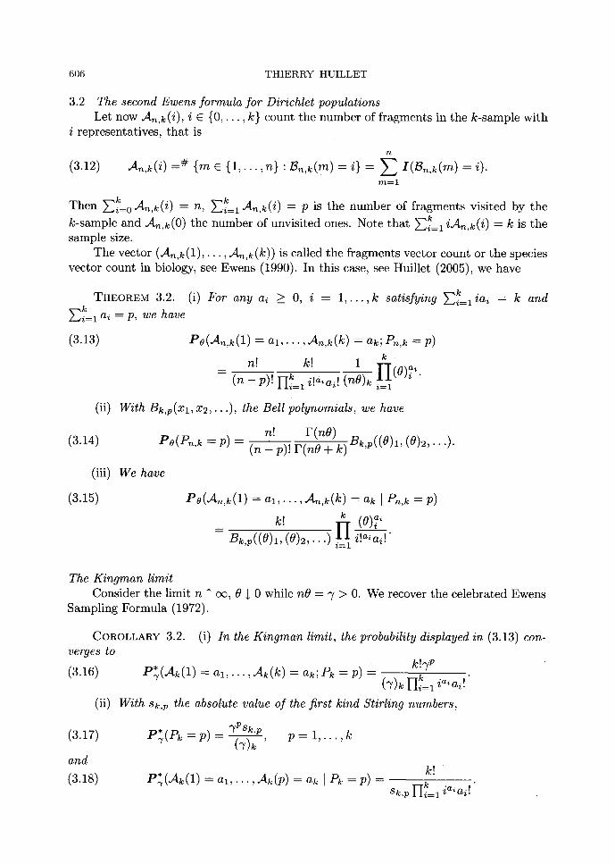
3.2 The second Ewens formula for Dirichlet populations Let now .An,k(i), i E {0 , . . . , k} count the number of fragments in the k-sample with

i representatives, that is

n

(3.12) A~,k(i) = # {m E {1, . . . , n } : Bn,k(m) = i} = E I ( ~ n , k ( m ) = i). m = l

k k Then ~-~i=o.An,k(i) = n, ~ i= l .An ,k ( i ) = p is the number of fragments visited by the k �9 k-sample and .An,k(O) the number of unvisited ones. Note that ~ i=1 W4n,k(~) = k is the

sample size. The vector (J tn,k(1) , . , . , An,k(k)) is called the fragments vector count or the species

vector count in biology, see Ewens (1990). In this case, see Huillet (2005), we have

THEOREM 3.2. (i) For any ai >_ 0, i 1 , . . . , k satisfying k = ~'~-i=liai = k and k ~-~i=l ai = p, we have

(3.13) Po(An,k(1) = a l , . . . , .An,k(k) = ak; P~,k = P) k �9

= n____~, v k! 1 1-[ (0) ~, ' ( n - p ) ! k I-Ii=1 i!alai ! (nS)k i=1

(ii) With Bk,p(X~, x2, . . . ) , the Bell polynomials, we have

n! F(n0) Bk,p((0)l , (0)2, . . . ) . (3.14) Pe(Pn,k -= p) - (n --- p)! F(nO + k)

(iii) We have

( 3 . 1 5 ) Po(An,k(1) = a l , . .. ,An ,k (k ) -~ ak I Pn,k = p )

B k , p ( ( O ) l , (O)2 , . . . ) ill.= i !a 'a i ! "

The Kingman limit Consider the limit n 1" oc, 0 I 0 while nO = y > 0. We recover the celebrated Ewens

Sampling Formula (1972).

COROLLARY 3.2. (i) In the Kingman limit, the probability displayed in (3.13) converges to

(3.16) P~(Ak(1) = e l , . . . ,Ak(k) = ak;Pk = p ) = kT~P I-L=I ia~ai !

(ii) With Sk,p the absolute value of the first kind Stirling numbers,

(3.17)

and

(3.18)

P.y(Pk = P) - 7PSk,p ' p = 1 , . . . , k

P~(Ak(1) = a l , . . . , . A k ( p ) = ak I Pk = P) = k! k

sk,p IIi=l ia~ai !


3.3 Donnelly- Tavard-Griffiths sampling formula for the Dirichlet partition We now consider sampling formulae from Dirichlet partitions for which the order in

which the consecutive fragments are being discovered in the sampling process matters. Consider a k-sample and let ml ~ m2 ~ . " ~ mp denote the ordered number of

the first, second, . . . , the p-th distinct animals sampled from Sn when only P,~,k = P distinct fragments were visited. Let Cn,k(q), q = 1, . . . ,p be the number of animals of the q-th species to appear. Using Theorem 2.1, we can prove (see Huillet (2005))

THEOREM 3.3. For any Cq >_ 1, q = 1 , . . . , p s a t i s f y i n g ~-~P cq = k and any p =

1 , . . . , n A k ,

(3.19) Po(Cn,k(1) = Cl, . . . ,Cn,k(P) = Cp; Pn,k = P) (k - 1)! F(1 + ( n - p + 1)0)r(0 + cp)

p-1 r(1 0)r((n + 1)0 + cp)F(cp) YIq=l ( k - E q ci) -~- - p

P-1 {r(1 + ( n - q + 1)O)F(O+cq) F ( ( n - q ) O + c q + l + . . . + C p ) } x H 1ToT -u :: "

q=l

Remark. (the law of succession) (i) Consider equation (3.19) and, with mr E { m l , . . . , rap}, let

P(Mk+I = m r I Cn,k(1) : C l , . . . , C n , k ( p ) : Cp; Pn ,k : P)

be the conditional probability that the (k + 1)-th sample is one from the previously encountered species already visited cr times. One can show, see Huillet (2005), that, as for the ESF,

(3.20) Po(Mk+l E species seen cr times I Cn,k(1) = c l , . . . ,Cn,k(p) = Cp; Pn,k : P)

0 +Cr -- n O + k '

which is again independent of Cq, q E {1, . . . ,p}\{r} and also of p. (ii) Summing over r = 1, . . . ,p, the conditional probability that Mk+l C {any one

of the species previously seen} is thus P O+c r = pO+k Taking its complement to 1, E r = l nO+k nOWk" we obtain

(3.21) Pe(Mk+l is new I Cn,k(1) = c l , . . . ,Cn,k(p) = Cp; Pn,k = P)

(n - p)e n O + k '

which is independent of cell occupancies Cl,. . . ,Cp but depends on the number p of distinct fragments already visited by the k-sample.

The Kingman limit Passing to the Kingman limit in Theorem 3.3 gives the celebrated Donnelly-Tavar~-

Griffiths sampling formula given in Donnelly and Tavar~ (1986), p. 10 (see Huillet (2005) for details).


COROLLARY 3.3. (i) In the K i n g m a n l imit , the probabili ty (3.19) converges to

(3.22) , k!~/p

P~(Ck(1) = c 1 , . . . ,Ck(p) = cp;Pk = p ) = (7)k Hq=l (Cq p -[- ' '" Jr- Cp)

(ii) With sk, p the absolute value of the f irst k ind S t i f l ing numbers ,

(3.23)

and

(3.24)

, ~PSk,p P ~ ( P k = P ) - (7)k ' p = l , . . . , k

P~(Ck(1) = C l , . . . , Ok(p) = Cp I Pk = p) : k!

P c Sk,p H q = l ( q "[- " ' ' "~ Cp)"

4. Intervals between new sampled species from Dirichlet partition

In this section, we shall consider the following sampling problem from Dirichlet parti t ion. From the knowledge of the order in which new fragments are being discovered, what can be said about the random number of samples separat ing the discovery of consecutive new fragments until exhaust ion of the list? We shall first consider the case of a fixed sample size k and then the case of an unl imited size.

Assume there are P~,k = P <_ n A k := k~ distinct species visited by the k-sample

drawn from S n d Dn(O), with k _> 2. Let m l 7 s . " 7 ~ mp be their fragments numbers in order of their appearance. Let :Dn,k(r), r = 1 , . . . , p - 1 be the sample size between the discovery of the r - th and the (r + 1)-th new fragments. Let X1 -- 1 and Xz =

l--1 l--[k=1 I ( M z 7 ~ Mk), 1 = 2 , . . . , k. This binary sequence takes the value 1 each t ime a new species is visited by the k-sample; otherwise its value is 0. Let dr _ 1, r = 1 , . . . ,p - 1,

p--1 r d . . dp := k - y ~ . r = l d r _> 1 and-dr = Y~q=l q, r = 1, . ,P, d0 := 0. The following two events are identical

and

"7:)n,k(1) = dl , . . . , :Dn,k(p -- 1) = dp-1; Pn,k = P"

"X1 : 1, X2 . . . . . Xdl : 0, X d l + l = 1, X d l + 2 . . . .

: X ~ 2 = O , . . . , X ~ p _ l + 1 : 1, XXv_~+ 2 . . . . . XX v O".

Next, from the above law of succession displayed in (3.21), with b l , . . . , bl E {0, 1} l, we get

Po(Xz+I = 1 I X1 = b l , . . . , X 1 = bl) =

Po(XI+I --- 0 I X1 = b l , . . . , X l = bl) --

Using this, we obtain

(n I - q=l bq)O

n O + l

l + 0 . ~-~l bq q = l

n O + l

p--1 THEOREM 4.1. Let p < kn. Wi th dr >_ 1, r = 1 , . . . ,p - 1, dp := k - }-~r=l dr _> 1 r

and -dr = ~-~q=l dq, r = 1 , . . . ,p, do := O, we get


(4.1)

(4.2)

(i)

(ii)

Po(:Dn,k(1) = dl , . . . , ~Dn,k(p - 1) = dp-1; Pn,k = P)

Opn! P = (n - p ) ! ( n O ) k l - I (1 -[- re nt-ar-1)dr-l"

r=l

Po(:Dn,k(1) = d l , . . . , D n , k ( p - 1) = dp-1 [ Pn,k = P)

Op P

= Bk,p((0)l, (0)2 , . . . ) H ( 1 + rO + a ~ - l ) a ~ - l .

PROOF. (i) We have:

Po(7:)n,k(1) = d l , . . . , l ) n , k ( p - 1) = dp-1; P~,k = P)

p--1 (n -- r)O P -&- i l + rO

= H ? r + n 0 " H H l + n O r=0 r=l /=d~-l+l

p--1 p dl_i1 _ 1 - [ ~ = 0 [ ( n - r)O] - I I +re)

- - r = l t=a._,+l

n! 0 p P ~-~ ~ (?~O)------k H (1 + rO + dr-X)d~-X,

r=l

(ii) follows from the expression (3.14) of P o ( P n , k = P). []

R e m a r k . (Waring distr ibution) Let us recall here some e lementary facts on Waring distr ibutions in the generalized hypergeometr ic of type B3 class. A discrete r andom variable W E {0, 1 , . . . } has Waring dis t r ibut ion W ( b , a) with parameters b > a > 0 if

P ( W = x) = ( b - a ~ (a)~ We have E ( W ) = a / ( b - a - 1) if b - a > 1, = +c~ if not. / (b)x+l " Regrouping the events "W > n ' , a random variable b W E { 0 , 1 , . . . ,n} has bounded

Waring dis t r ibut ion b W ( n , b, a) if P ( b W - x) = (b - ~J (b--52~+~ ' ~ (a)~ if x �9 {0, 1, . . . ,n -- 1},

P ( b W - - n ) = (a)n i f b W = n . We o b t a i n E ( b W ) = a ( 1 - (a+l)~) i f b C a + l and b-a-1 (b)~ E ( b W ) = (b - 1)[~'(b + n) - ~'(b)] if b -- a + 1, where r := r ' ( b ) / r ( b ) .

One may check that if W d W ( b , a), then W d geom(beta(a , b - a)) where G d geom(p) is a geometrically dis t r ibuted random variable with law P ( G = x) = p~(1 - p ) ,

x _> 0. Here, p is the random success probabili ty, with p d be ta(a , b - a), independent of G. From this, we get

r(b) .~1 pX+a-1 P ( W = x ) - r(a)r(b- a) - . (1 - p ) b - a d p

P(b) P(a + x)V(b - a + 1) = (;b , (a)~ = r ( a ) r ( b - a ) r ( b + x + 1) - a~ (b -~+ l"

610 THIERRY HUILLET

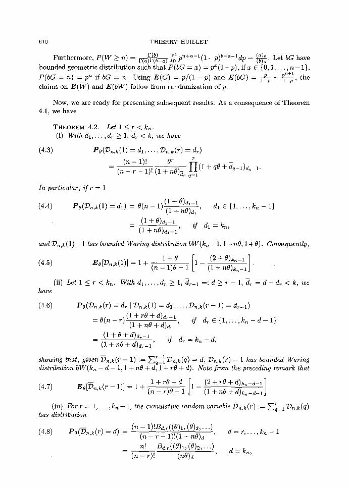
Fur thermore , P ( W > n) -- r(b) r(~)r(b-~) foP~+~-l( 1-p)b-~-ldp = (~)~ Let bG have - ( b ) ~ "

bounded geometr ic d is t r ibut ion such t ha t P(bG = x) = pX(1 - p ) , if x �9 {0, 1 , . . . , n - 1}, P(bG = n) = p n i f b G = n. Using E ( G ) - - p / ( 1 - p ) and E(bG) = 1-p p - p~+~l-p, the claims on E ( W ) and E ( b W ) follow from randomiza t ion of p.

Now, we are ready for present ing subsequent results. As a consequence of T h e o r e m 4.1, we have

(4.3)

THEOREM 4.2. Let 1 <_ r < k~. (i) With d l , . . . , d r >_ 1, dr < k, we have

Pe(~n ,k (1) = d ] , . . . , :Dn,k(r) = dr)

( n - 1 ) ~ O r r

-- ( # = 7 - 1 ) ! (1 + nO)~ H (1 + qO + ~ - 1 ) ~ - 1 . q=l

In particular, i f r = 1

(4.4) Pe(T)~,k(1) = dl) = 0(n - 1)(1 + 0)dl-1 (1 + nO)d1 ' dl �9 { 1 , . . . , kn - 1}

_ ( I + 0 ) d l _ I i f d l = k ~ , (1 + nO)~- l '

and D n , k ( 1 ) - 1 has bounded Waring distribution b W ( k ~ - 1, 1 +nO, 1 +8). Consequently,

1+8 [1_ (2+0)k_i] (4.5) E0[:D~,k(1)] = 1 + (n - 1)8 - 1 (1 + nO)k~-i "

(ii) Let 1 < r < kn. With d l , . . . , d r >_ 1, d r -1 = : d > r - l , dr = d + d r < k, we have

(4.6) Po(~Dn,k(r) -- dr ] ~ , , k (1 ) = d l , . . . ,Dn,k(r -- 1) = d r_ l )

(1 + rO + d)d~-l , = O(n -- r) -(i-+--nO+d--~d~ i f dr �9 { 1 , . . . , kn - d - 1}

(1 + 0 + d)dr-1 = ( l + n O + d ) d ~ - l ' i f d r = k n - d ,

- - r--1 showing that, given ~ ) n , k ( r -- 1) :---- ~ q = l ~ ) n , k ( q ) = d, ~ ) n , k ( r ) -- 1 h a s b o u n d e d Waring distribution bW(kn - d - 1, 1 + nO + d, 1 + rO + d). Note from the preceding remark that

- - l + r 0 + d [ 1 - ( 2 + r O + d ) k ~ - d - l l (4.7) Ee[:Dn,k(r - 1)] = 1 + ( n - - r ) 0 - 1 (1 + nO §

r (iii) For r = 1 , . . . , kn - 1, the cumulative random variable ~n ,k (r ) := ~ q = l T)n,k(q) has distribution

(4.8) Po(~n , k ( r ) = d) = (n - 1)!Bd,r((0)l , (0)2 , . . . ) ( n - - r - 1)!(1 + n 0 ) d ' d = r , . . . , k ~ - 1

= n! Bd,r((O)l, (8)2 , . . . ) d = kn, (n - ~)! (no)d '

SAMPLE F R O M D I R I C H L E T PARTITION 611

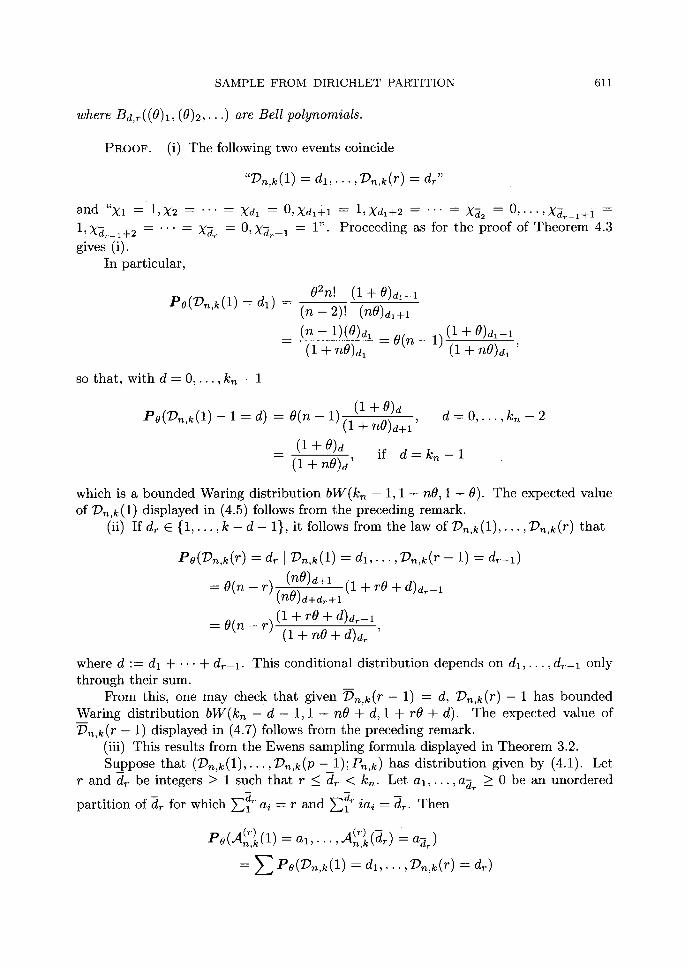
where Bd,~( ( O)l , (8)2 , . . . ) are Bel l po lynomia ls .

PROOF. (i) The following two events coincide

" Z ) n , k ( 1 ) - - d l , . . . , T ) n , k ( r ) = d r "

and "X1 = 1 , X 2 . . . . . Xd~

1, X~_~+2 . . . . . X~ = O, X~+I = 1". gives (i).

In particular,

P o ( ~ n , k ( 1 ) = d l ) --

= 0, Xdl+l : 1, X d l + 2 . . . . . X~ 2 = 0 , . . . ,X~r_l+l : Proceeding as for the proof of Theorem 4.3

02n! (1+0)~1_1

( n - 2)! (n0)dl+l ( n - 1)(0)dl - - 0 ( n - - l ) ( l + n 0 ) d l

( 1 + 8 ) 4 1 - 1 (1 + nO)d1 '

so that , with d ---- O, . . . , k n - 1

(1 + O)d d = O , . . . , k ~ - 2 Po(Z)n ,k (1 ) - - 1 = d) = O(n - 1)(1 + nO)d+l '

_ ( l + 0 ) d if d = k ~ - I (1 + nO)d'

which is a bounded Waring dis t r ibut ion b W ( k ~ - 1, 1 + nO, 1 + 0). The expected value of Dn,k(1) displayed in (4.5) follows from the preceding remark.

(ii) If dr C { 1 , . . . , k - d - 1}, it follows from the law of :D~,k(1), . . . , ~ , k ( r ) tha t

Po(Z)n ,k ( r ) = dr ]/)n,k(1) = d l , . . . , T ) n , k ( r - - 1) = d r - i )

(nO)d+l (1 + r e + d)d~- i = O(n -- r) (nO)d+d~+l

= O(n - r ) ( 1 + rO + d )d~- i ( l + n 0 + d ) d ~ '

where d := dl + �9 �9 �9 + dr-1. This condit ional dis tr ibut ion depends on dl, �9 �9 �9 dr-1 only through their sum.

From this, one may check that given : D n , k ( r - 1) = d, T~n,k(r) -- 1 has bounded Waring dis t r ibut ion b W ( k n - d - 1, 1 + n0 + d, 1 + rO + d). The expected value of :D~,k(r -- 1) displayed in (4.7) follows from the preceding remark.

(iii) This results from the Ewens sampling formula displayed in Theorem 3.2. Su_ppose tha t (:Dn,k(1),.. . ,:D~,k(p--_1); P~,k) has dis t r ibut ion given by (4.1). Let

r and dr be integers _> 1 such that r _< dr < k~. Let a l , . . . , a - ~ > 0 be an unordered

par t i t ion of dr for which E 1 ai = r and ~-~-1 iai = dr. Then

P o (~) (~) - (An,k(1) = a~, . .. , A n , k ( d ~ ) = a-~)

: E Po(~)n'k(1) : d l , . . . , ~ ) n , k ( r ) = dr)

612 THIERRY HUILLET

where summat ion runs over all distinct ordered part i t ions d l , . . . , dr of dr which give rise to the unordercd par t i t ion a l , . . . , aa~ of dr. From (4.3), we get

(r) (r) - Po(An,k(1) = a l , . . . ,Mn,k(d~) = aa~)

a~ = n. T _ __dr! 1 H ( O ) ~

(n- r)! i>ai! (nO)a if dr = k~

(n-_l__)~ _ __dr' 1 H(0 )~ ~ if r < dr < k~ ( n ~ 7 )I Hd,.1 i!aiai ! (1 + nO)~ i----1

with

_ __ar

~d~_l i!a, afl .=

Next, for d = r, r + 1 , . . . , kn - 1, we have

=Ba~,r((eh,(O)~,...).

Po(~n,k(r) d) E (r) (r) = = Po(An,k(1) = a l , . . . ,A~,k(d ) = a4)

d . where summat ion runs over ai > 0 satisfying ~-~d ai = r and ~-~-1 zai ---- d. []

Lastly, we shall turn to the related question of comput ing the law of l)n(r), the sample size separat ing consecutive visits to the r - th and the (r + 1)-th new species, when sampling is from Dn(O) with unlimited sample size. For this problem, we obtain

THEOREM 4.3. L e t 1 <_ r < n - 1.

(i) The law of T)n(r) is given by

(4.9) Po(7)n(r) > d ) =

• I I ~ F ( l + ( n - q + l ) O ) q=l t r (1 + 0 ) r ( (n - q)O)

P(1 + 0 + kq)r((n - q)O + kq+~ + . . . + kr) ]

and the following stochastic domination property holds

~)n(r) ~ ~)n(r-- 1).

(ii) With 1 < r < n - 1, the mean value of TPn(r) reads

(4.10) Eo(~)n(r)) = ~ I ( n - q + l ) O q=l (n q)O- l '

= +oc, if not.

if ( n - r ) e > l

S A M P L E F R O M D I R I C H L E T P A R T I T I O N 613

PROOF. (i) Given Sn, w e have

P(I)n(r ) > d [ M; -: m l , . . . , M~r -: mr, Sn) = Smq

since, if :Dn(r) > d, at least d sample need to fall in the already visited fragments. Averaging over Sn and summing over all realizations m l r . . . ~ mr of M ~ , . . . , Mr', we get

Developing with the help of the mult inomial ident i ty and using the joint moment function of L 1 , . . . , L ~ , as obtained from (2.11), gives the result. The stochastic dominat ion

r r--1 proper ty :Dn(r) h :D~(r - 1) follows from the fact tha t (Y~q=l Lq) d >- (~-]q=l Lq) d which is maintained when taking the expectation.

r (ii) Concerning the mean value of :Dn(r), recalling 1 - ~q=l Lq -- 1-Iq=l vq where

Vq, q = 1 , . . . , r are independent with l a w Yq d b e t a ( ( n - q)O, 1 + 0) we have from (4.11)

r Eo(:D~(r)) = E Po(:Dn,k(r) > d) = Eo 1 - ~q=X Lq d_>0

(<) n ---: S . : E Yq q--1

(n - -q+l )O The expected value of E o ( ~ ) is finite and equal to %-q)0-i if and only if (n - q)O > 1.

We note tha t when r > n -O -1 is such tha t (n-r)O < 1, the expected t ime separat ing the visit from the r - th to the (r + 1)-th new fragment becomes infinitely large. In particular, for values of 0 such tha t O < 1/(n - 1), Eo(:Dn(r)) = c~ for each 1 < r < n - 1. On the contrary, if O ~ 1, Eo(:Dn(r)) < oo for each 1 ~ r < n - 1.

Note tha t , if (n - r)O > 1, since 0 > 0

Ee(:D~(r)) - (n - r + 1)O Eo(:D~(r _ 1)) > Ee(:Dn(r - 1)). (n r)O --1

The expected visiting t imes sequence to consecutive new species, when these exist (when they are finite), is an increasing one, as conventional wisdom suggests. These results are consistent with the ones of Huillet (2003), obtained in the part icular case 0 = 1, namely

(-[ n - q + l _ n ( n - 1 ) Eo=l(:Dn(r)) q=illn q- I (n- r)(n- r- l)'

for e a c h l < r < n - l . [ ]

k Remark. With ~q=l q -- d, the following te rm arising from (4.9)

( d ) ~ i r ( l + ( n - q + l ) O ) F ( l + O + k q ) r ( ( n - q ) O + k q + l + . . . + k r ) k l , . . . , kr r(1 + e ) r ( ( n - q)0)r(1 + (n - q + 1)0 + kq + . . . + k~)

q = l


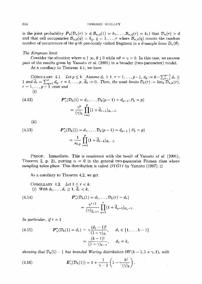
is the joint probabil i ty Po(l)n(r) > d; Bn,d(1) = k l , . . . , ]3n,d(r) = kr) t ha t ~)n(r) > d and tha t cell occupancies 13~,d(q) = kq, q = 1 , . . . , r where ~n,d(q) counts the random number of occurrences of the q-th previously visited fragment in a d-sample from Dn (0).

The Kingman limit Consider the si tuat ion where n T oc, 0 $ 0 while nO = -y > 0. In this case, we recover

par t of the results given by Yamato et al. (2001) in a broader (two-parameter) model. As a corollary to Theorem 4.1, we have

COROLLARY 4.1. Letp < k. Assume dr ~ 1, r -- 1 , . . . , p - l , dp := k-~-~rP__-~ dr _> r 1 and-dr = ~-~q=l dq, r = 1 , . . . ,p, d0 := 0. Then, the weak limits iOk(r) := l im. T)n,k(r),

r = 1 , . . . , p - - 1 exist and (i)

(4.12)

(ii)

(4.13)

P~(7)k(1) = d l , . . . , / ) k ( p - - 1) = dp-1;Pk = P)

__ ~ P P

H(1 + r = l

P~(T)k(1) = d l , . . . ,TPk ( p - - 1) = dp-1 ] Pk = P)

1 P = H(1 +ar_l)d _1.

8k'p r=l

PROOF. Immediate. This is consistent wi th the result of Yamato et al. (2001), Theorem 2, p. 21, put t ing a = 0 in the general two-parameter P i tman class where sampling takes place. This distr ibution is called D T G I I by Yamato (1997). []

As a corollary to Theorem 4.2, we get

(4.14)

COROLLARY 4.2. Let 1 < r < k. (i) With d l , . . . , d r >_ 1, dr < k,

P~(:Dk(1) = d l , . . . , / ) k ( r ) = dr)

( " / )d , .+ l = (1 -[- dq-1)dq_ 1.

, ( d l - 1 ) ! dl e { 1 , . . , k - l } (4.15) P.~(/)k(1) = d l ) --- ? (1 + V)dl' '

(k - 1)! (1 + V)k-1 dl = k,

showing that T)k(1) -- 1 has bounded Waring distribution bW(k - 1, 1 + V, 1), with

(4.16) E.r(Dk(1)) = 1 + 1 1 - "y . " / - 1

In particular, if r = 1


(ii) Let 1 < r < k. With d l , . . . , dr >_ 1, -dr-1 =: d > r - 1, -dr = d + dr < k,

(4.17) P.~(Dk(r) = d~ I :Dk(1) = d l , . . . , Dk(r -- 1) = d r - l )

(1 + d ) d . - I if

= "/(1 + ' y + d)d~' (1 + d)k -d -1

(1 + 7 + d ) k - d - l '

- - r - - 1 showing that, given Dk ( r -- 1) := ~ q = l 7?k(q) = d, 7?k(r) -- 1 has bounded Waring distribution b W ( k - d - 1, 1 + ~/ + d, 1 + d). In particular,

d r E { 1 , . . . , k - d - 1 }

if d ~ = k - d ,

( (4.18) E , :Dk(r)

= 1 +

(iii) For r = 1 , . . . , k - 1, the bution

(4.19) P.~(l)k(r) = d) -

) E Z ) k ( q ) = d q=l

l + d ( 1 - ( 2 + d ) k - d - 1 ) - 1 (1 ~- ~ /+ d ) k - d - 1 "

- - r cumulative variable T)k(r) := ~-~q=l T)k(q) has distri-

r

~/ Sd,r d = r , r + l , . . . , k - 1 (1 + 7)d '

- - r s ")1 d,r d = k,

(~)d '

where Sd,~ are the absolute values of f irst kind Stif l ing numbers.

PROOF. Immediate . These are again consistent with results of Yamato et al. (2001), as from Theorem 3, Proposit ions 3 and 4, put t ing a = 0 in their formula. []

Finally, as a corollary to Theorem 4.3, we easily obtain

COROLLARY 4.3. Let r >_ 1. (i) The law of T)(r) := l im.:Dn(r) is given by

(4.20) P~(~) ( r ) > d) = 7~d! 1 r

Z IIq=l{-r + kq + + kr} < ..... k~_>o:~[ kq=d

and the following stochastic dominat ion property holds

D(r ) >- D( r - 1).

(ii) With 1 < r, the mean value of D(r ) reads

(4.21) E~(~ (r ) ) = , if ~ > 1

= + ~ , /f 0 < '~ <_ 1.

616 THIERRY HUILLET

PROOF. Immediate from Theorem 4.3. []

Remark. With ~-~=1 kq -= d, kq >_ O, the following term arising from (4.20)

~rd! 1 r

IIq=l{ + 4 + + kr}

is the joint probability P~(T)(r) > d; Bd(1) = k l , . . . , Bd(r) = kr) that :D(r) > d and that cell occupancies are Bd(q) = kq, q = 1 , . . . , r, where Bd(q) counts the random number of occurrences of the q-th previously visited fragment in a d-sample from GEM(~/) .

REFERENCES

Barrera, J., Huillet, T. and Paroissin, C. (2005). Size-biased permutation of Dirichlet partitions and search-cost distribution, Probability in the Engineering ~ Informational Sciences, 19(1), 83-97.

Donnelly, P. (1986). Partition structures, Pblya urns, the Ewens sampling formula and the age of alleles, Theoretical Population Biology, 30, 271-288.

Donnelly, P. (1991). The heaps process, libraries and size-biased permutation, Journal of Applied Probability, 28, 321-335.

Donnelly, P. and Tavar@, S. (1986). The age of alleles and a coalescent, Advances in Applied Probability, 18, 1-19.

Ewens, W. J. (1972). The sampling theory of selectively neutral alleles, Theoretical Population Biology, 3, 87-112.

Ewens, W. J. (1990). Population genetics theory--the past and the future, Mathematical and Statistical Developments of Evolutionary Theory (ed. S. Lessard), Kluwer, Dordrecht.

Ewens, W. J. (1996). Some remarks on the law of succession, Athens Conference on Applied Probability and Time Series Analysis (1995), Vol. I, Lecture Notes in Statistics, 114, 229-244, Springer, New York.

Huillet, T. (2003). Sampling problems for randomly broken sticks, Journal of Physics A, 36(14), 3947- 3960.

Huillet, T. (2005). Sampling formulae arising from random Dirichlet populations, Communications in Statistics: Theory and Methods (to appear).

Huillet, T. and Martinez, S. (2003). Sampling from finite random partitions, Methodology and Comput- ing in Applied Probability, 5(4), 467-492.

Kingman, J. F. C. (1975). Random discrete distributions, Journal of the Royal Statistical Society. Series B, 37, 1-22.

Kingman, J. F: C. (1993). Poisson Processes, Clarendon Press, Oxford. Pitman, J. (1996). Random discrete distributions invariant under size-biased permutation, Advances in

Applied Probability, 28, 525-539. Pitman, J. (1999). Coalescents with multiple collisions, Annals of Probability, 2T(4), 1870-1902. Pitman, J. (2002). Poisson-Dirichlet and GEM invariant distributions for split-and-merge transformation

of an interval partition, Combinatorics, Probability and Computing, 11(5), 501-514. Pitman, J. and Yor, M. (1997). The two parameter Poisson-Dirichlet distribution derived from a stable

subordinator, Annals of Probability, 25, 855-900. Sibuya, M. and Yamato, H. (1995). Ordered and unordered random partitions of an integer and the

GEM distribution, Statistics ~ Probability Letters, 25(2), 177-183. Tavar@, S. and Ewens, W. J. (1997). Multivariate Ewens distribution, Discrete Multivariate Distribu-

tions (eds. N. L. Johnson, S. Kotz and N. Balakrishnan), 41,232-246, Wiley, New York. Yamato, H. (1997). On the Donnelly-Tavar@-Griffiths formula associated with the coalescent, Commu-

nications in Statistics: Theory and Methods, 26(3), 589-599. Yamato, H., Sibuya, M. and Nomachi, T. (2001). Ordered sample from two-parameter GEM distribu-

tion, Statistics 8J Probability Letters, 55(1), 19-27.

unordered and ordered sample from dirichlet distribution · (1 - v1)v2. iterating, the final sbp of...

Documents