: s

Discussion Paper available online : http://fdef.uni.lu/index.php/fdef_FR/economie/crea

CCCRRREEEAAA DDDiiissscccuuussssssiiiooonnn

PPPaaapppeeerrr

222000111444---111444

Differential Games with (A)symmetric Players

and Heterogeneous Strategies (II)

available online : http://wwwfr.uni.lu/recherche/fdef/crea/publications2/discussion_papers

Benteng Zou, CREA, Université de Luxembourg

August, 2014

For editorial correspondence, please contact: crea@uni.lu University of Luxembourg

Faculty of Law, Economics and Finance 162A, avenue de la Faïencerie

L-1511 Luxembourg

Center for Research in Economics and Management University of Luxembourg

The opinions and results mentioned in this paper do not reflect the position of the Institution

CREA Discussion

Differential Games with (A)symmetric Playersand Heterogeneous Strategies (II)∗

Benteng Zou †

CREA, University of Luxembourg

Abstract

One family of heterogeneous strategies in differential games with (a)symmetric

players is developed in which one player adopts an anticipating open-loop strategyand the other adopts a standard Markovian strategy. Via conjecturing principle,

the anticipating open-loop strategic player plans his strategy based on the possi-

ble updating the rival player may take. These asymmetric strategies frame non-

degenerate Markovian Nash Equilibrium, which can be subgame perfect. Except

the stationary path, this kind of strategy makes the study of short-run trajectory

possible, which usually are not subgame perfect. However, the short-run non-

perfection provides very important policy suggestions.

Keywords: Differential game, subgame perfect Markovian Nash Equilibrium, Het-

erogeneous strategy, anticipating open-loop strategy.

JEL classification: C73, C72.

∗I gratefully acknowledge the useful and inspiring discussions with Luisito Bertinelli, RaoufBoucekkine, Herbert Dawid, Engelbert Dockner, Gustav Feichtinger, Yutao Han, Luca Marchiori, PatricePieretti, Jennifer Reiganum, Ioana Salagean, and Ingmar Schumacher, in early stages of this study. I alsoacknowledge the support of COST Action IS1104: The EU in the new economic complex geography: models,tools and policy evaluation.†Address: 162a, Avenue de la Faıencerie, L-1511 Luxembourg, Luxembourg. E-mail: ben-

teng.zou@uni.lu

1

1 Introduction

As stated in the seminal paper of Reinganum and Stokey (1985, p.162) “when formulat-ing a model, care should be taken to choose a strategy space that is appropriate for the situationunder study. Path strategies may be appropriate in some situations, decision rule strategies inothers, and intermediate formulations in still others.” More recently, Dockener et al. (2000,p.87) emphasize again that the analysis should “ · · · consider equilibria in which some ofthe players represent their optimal control paths in open-loop form while others choose non-degenerate Markovian strategies. ” and further ” · · · the choice to solve a differential game· · · ( for equilibria in which some players use open-loop strategies while others employ non-degenerate Markovian strategies) is part of the modelling stage and one should try to analyzethat equilibrium which describes best the situation at hand.”

This paper takes special care of these intermediate formulations in differential gameswhere all players share the same information structure1. Nevertheless, heterogeneitymay appear in different aspects.

First, players share the same information set, however, they may have difficulties toperform the same strategies as their rivals. Dawid and Feichtinger (1996) show suchasymmetric case in the study of optimal allocation of drug control efforts (see Section3 for more detail). In their model, both government (the drug controller) and drugdealers know the drug users. But their strategy spaces may differ. Han et al. (2014)present another such kind of situation in dynamic tax competition between large andsmall economies. As they argued that the small economy may be less efficient thanthe large one in interpreting its policy and offering public services, while the smalleconomy may be more flexible than its large rival in collective or single-minded action.

Second, though players share the same information and have the same capacities tointerpret the same strategies or policies as their rivals, they may differ in their moralstandard or their attitudes. In other words, players can be symmetric in their character-istics but just play asymmetric strategies. This can be seen from the international CO2

1See more detail in Section 6.2 of Bacard and Olsder (1998)

2

emission control problem. Despite the well-known ”tragedy of the commons” results,unilateral action has been observed in collective-action problems like climate-changenegotiations. Notable in 2007, EU country representatives committed themselves toa unilateral 20 per cent reduction in GHG emissions by 2020 and even offered a 30per cent decrease in case an international agreement could be found. While the otherbig players (like the USA and China) can deviate from their commitments (or do notcommit at all) and regularly revise their targets and policies. Indeed, under a differentsetting, Reinganum (1981) shows that under her setting two identical players adoptingasymmetric strategies is optimal.

Thus, player engaging in this kind of differential games must first figure out that,among other important issues, in which strategy space he is playing, the subgame per-fection of the chosen strategies and the possibility of studying the trajectory dynam-ics. Via conjecturing principle, we shall introduce heterogeneous strategies by allowingsome players to adopt open-loop strategies while others non-degenerate Markovianstrategies.

The main contribution of this work is that Hamiltonian can be applied to look for het-erogeneous strategic Nash Equilibrium along the whole trajectory. The conjecturingprinciple makes this possible. Otherwise, without this guessing principle, applyingHamiltonian searching for feedback strategies, we will face the difficulties of guess-ing each others’ infinitely many optimal strategies, as clearly stated by Kamien andSchwartz (2003, P.275): ” finding player i’s optimal feedback strategy u∗i (x, t) requires thatplayer j’s optimal feedback strategy u∗j(x, t) be known which, in turn, requires that player i’soptimal be known, and so on.” The family of games, where one player is less flexibleof changing strategies based on state of the world than the other player, makes thisguessing process stop at one step instead of infinitely many.

Our approach fits specially well to differential games with unilateral commitment (seemore in the Section 3). Most of the economic literature2 applying differential gamesignores the impact of unilateral commitment and focuses only on symmetrical strategyspaces. Nevertheless, unilateral commitment is not the only case where these kinds

2See Long (2010) for a recent and complete survey

3

of heterogeneous strategies are adopted. In Section 3, we present different situationswhere this kind of strategy space should be taken. Thus far, the literature providesonly limited applications of these kinds of heterogeneous strategies. The technique weare going to present is also studied by Dockener et al. (2000; Example 4.1) where thereare two asymmetric players with different objective functions though sharing the samestate equation.

The paper is organized as follows: in Section 2, we introduce the concept and formula-tion of heterogeneous strategy in a general setting. Then, Section 3 presents some situ-ations where anticipating open-loop and non-degenerate Markovian strategies shouldbe played at the same time. And as an example of further development and mathe-matics exercise of calculating the strategy, in Section 4, we restudy the seminal modelof Fershtman and Kamien (1987)–dynamic duopolistic competition with sticky prices, inwhich they study the duopolistic competition through time under the assumption thatthe price of a homogeneous product does not adjust instantaneously to the price indi-cated by its demand function at the give level of output. By applying the heterogenousstrategies developed in Section 2, we can conclude that (i) a different stationary sub-game perfect Markovian Nash equilibrium is obtained; (ii) the results of limit gamefrom heterogenous strategies lie between Fershtman and Kamien (1987)’s symmetricopen-loop and symmetric Markovian Nash equilibria: in the limit game, the steadystate price from heterogenous strategies is strictly higher than the price from sym-metric Markovian Nash equilibrium and strictly lower than the price from symmetricopen-loop (which is the same as in the static Cournot equilibrium). Some concludingremarks are given in Section 5.

2 Heterogeneous strategies

Consider a two-player differential game. Each player i(= 1, 2) chooses ui ∈ Ui (whereUi ∈ R is the choice space for player i) to maximize her objective function Πi:

maxui

Πi(ui, uj) = maxui

∫ ∞0

e−rtfi(t, ui, uj, x(t))dt, i, j = 1, 2, i 6= j,

4

where player j′s strategy uj ∈ Uj is taken as given by player i. We assume x(t) ∈ X isthe shared common state of the system 3 (withX ∈ R, the state space) and r is a positiveconstant denoting time preference and is the same for both players for simplicity. Thestate of the system is given by the following differential equation

x(t) = g(t, u1(t), u2(t), x(t)),∀t ≥ 0 (1)

with initial condition x(0) given. For simplicity, we also assume both objective func-tions fi(·) and state function g(·) are smooth functions.

For this differential game, we define the heterogeneous strategy as:

Definition 1 (Heterogeneous Strategic Nash Equilibrium) A 2-tuple (Ψ1,Ψ2) of func-tions Ψ1 : X × [0,+∞) → R and Ψ2 : [0,+∞) → R, with Ψ1 = Ψ1(x, t),∀(x, t) ∈X × [0,+∞) and Ψ2 = Ψ(t), ∀t ∈ [0,+∞), is called a Heterogeneous Strategic Nash Equilib-rium if, for each i = 1, 2, an optimal control path ui of player i exists and is given by: Markovianstrategy for player 1, u1(t) = Ψ1(x(t), t), and open-loop strategy for player 2, u2(t) = Ψ2(t).

In other words, player 1 adopts a Markovian strategy and its optimal choice u1 dependsnot only on time t, but also on the current state x of the system; while player 2’s optimalstrategy u2 depends only on time, i.e., there is an irrevocable commitment, which isgiven based on some anticipating of the rival player’s potential Markovian choice.

In the following, we build the principle of conjecturing on the guessing technique4.In short, the equilibrium is framed based on two stages: stage one is an imaginarystage and no game is really played. However, at this stage the players suppose thatboth of them adopt open-loop strategies based on Pontryagin’s Maximum principle,which would provide information for choosing their real strategies in the next stageand conjecturing the other player’s strategy. At stage two, the real game starts, playersadopt strategies based on their calculated information from stage one.

3Except some players commit on all the state variables, the concept and method may not be anal-ogous if there were different states for different players or multiple states, see for example Reynolds(1987).

4Guessing technique is often in use in game study, see Long (2010) for more examples.

5

To be more precise, the process is the following:

Stage 1. Given Pontryagin’s Maximum principle can offer optimal solution for eachplayer’s optimal control problem provided some sufficient conditions (i.e., concavityof objective functions and state equations) are checked, we can write down player i’sHamiltonian function as

Hi(x, λi, ui, t) = fi(t, ui(x, t), u∗j(t), x) + λi(t)g(t, ui(x, t), u

∗j(t), x), i = 1, 2, i 6= j.

Here u∗j(t) is player j’s optimal choice and taken as given by player i, λi is player i’scostate variable.

The usual first order conditions present the optimal solution for each player whichalso perform the open-loop strategies. Denote these optimal open-loop strategies as:Ψ1(t) = Ψ1(x(t), t) and Ψ2(t) = Ψ2(x(t), t), ∀t ≥ 0.

This step is essential for completing this process of heterogeneous strategy.

Stage 2. Player 1 (the Markovian strategic player) takes player 2’s (open-loop) strategyΨ2(t) as given, and hence, faces the following optimization problem:

maxu1(x,t)

∫ ∞0

e−rtf1(t, u1(x, t),Ψ2(t), x)dt,

subject to x(t) = g(t, u1(x(t), t),Ψ2(t), x(t)).

(2)

The corresponding current-value Hamiltonian for player 1 is

H1(x, λ1, u1, t) = f1(t, u1(x, t),Ψ2(t), x) + λ1(t)g(t, u1(x, t),Ψ2(t), x),

where λ1 denotes player 1’s costate variable.

Player 2, the open-loop strategy player, applies the conjecturing principle: player 2

guesses that the strategy of player 1 with the following modification: player 2 guessesthat strategy Ψ1(t) = Ψ1(x(t), t) will be replaced by Ψ1(x, t) with any state variablex ∈ X , since player 1 plays Markovian strategy. Therefore, player 2’s conjecturingof player 1’s strategy is: Ψ1(x, t) for any (x, t) ∈ X × [0,∞).

6

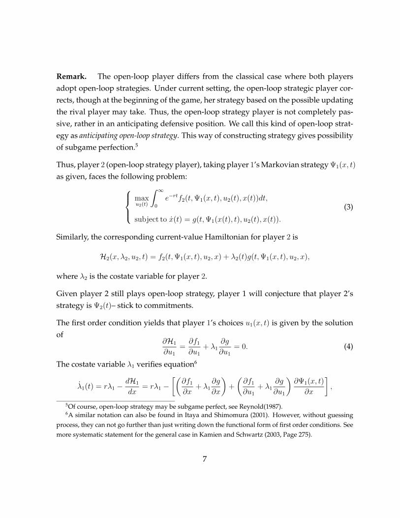
Remark. The open-loop player differs from the classical case where both playersadopt open-loop strategies. Under current setting, the open-loop strategic player cor-rects, though at the beginning of the game, her strategy based on the possible updatingthe rival player may take. Thus, the open-loop strategy player is not completely pas-sive, rather in an anticipating defensive position. We call this kind of open-loop strat-egy as anticipating open-loop strategy. This way of constructing strategy gives possibilityof subgame perfection.5

Thus, player 2 (open-loop strategy player), taking player 1’s Markovian strategy Ψ1(x, t)

as given, faces the following problem:maxu2(t)

∫ ∞0

e−rtf2(t,Ψ1(x, t), u2(t), x(t))dt,

subject to x(t) = g(t,Ψ1(x(t), t), u2(t), x(t)).

(3)

Similarly, the corresponding current-value Hamiltonian for player 2 is

H2(x, λ2, u2, t) = f2(t,Ψ1(x, t), u2, x) + λ2(t)g(t,Ψ1(x, t), u2, x),

where λ2 is the costate variable for player 2.

Given player 2 still plays open-loop strategy, player 1 will conjecture that player 2’sstrategy is Ψ2(t)– stick to commitments.

The first order condition yields that player 1’s choices u1(x, t) is given by the solutionof

∂H1

∂u1=∂f1∂u1

+ λ1∂g

∂u1= 0. (4)

The costate variable λ1 verifies equation6

λ1(t) = rλ1 −dH1

dx= rλ1 −

[(∂f1∂x

+ λ1∂g

∂x

)+

(∂f1∂u1

+ λ1∂g

∂u1

)∂Ψ1(x, t)

∂x

],

5Of course, open-loop strategy may be subgame perfect, see Reynold(1987).6A similar notation can also be found in Itaya and Shimomura (2001). However, without guessing

process, they can not go further than just writing down the functional form of first order conditions. Seemore systematic statement for the general case in Kamien and Schwartz (2003, Page 275).

7

where dH1

dxdenotes the total derivative7 of H1 with respect to x and the last term is

equal to zero, by the first order condition (4). Thus, player 1’s co-state equation reads

λ1(t) = rλ1(t)−(∂f1∂x

+ λ1(t)∂g

∂x

)(5)

with transversality condition limt→∞

e−rtλ1(t)x(t) = 0.

Similarly, u2(t), the optimal choices of player 2, is given by

∂H2

∂u2=∂f2∂u2

+ λ2∂g

∂u2= 0. (6)

And, the costate equation is

λ2(t) = rλ2 −dH2

dx= rλ2 −

[(∂f2∂x

+∂f2∂u1

∂Ψ1(x, t)

∂x

)+ λ2

(∂g

∂x+

∂g

∂u1

∂Ψ1(x, t)

∂x

)]or equivalently,

λ2(t) = rλ2 −[(

∂f2∂x

+ λ2∂g

∂x

)+

(∂f2∂u1

+ λ2∂g

∂u1

)∂Ψ1(x, t)

∂x

]. (7)

The associated transversality condition is limt→∞

e−rtλ2(t)x(t) = 0.

Remark. Equation (7) differs from (5) due to the fact that in (5) the first order condition(4) can be applied; while in (7), that is not possible.

Denote the solution of (4) and (6) as u∗1 = Ψ∗1(x, t),∀(x, t) ∈ X × [0,∞) and u∗2 =

Ψ∗2(t),∀t ≥ 0, respectively. To be more precise Ψ∗1(x, t) is a function of state x, thecostate variable evaluated at time t; and Ψ∗2(t) is a function of state and costate vari-ables both evaluated at t, thus, Ψ∗1(x, t) = Ψ∗1(x, λ1(t), t) and Ψ∗2(t) = Ψ∗2(x(t), λ2(t), t).Substituting these two into the Hamiltonian, we can readily check that the maximizedHamiltonianH∗1(x, λ1, t) andH∗2(x, λ2, t) are given by

H∗1(x, λ1, t) = f1(t,Ψ∗1(x, λ1, t),Ψ

∗2(x, λ2, t), x) + λ1 g(t,Ψ∗1(x, λ1, t),Ψ

∗2(x, λ2, t), x)

7The state variable affects the current-value Hamiltonian via two different ways: the direct impactsby the state equation and indirect impacts due to the strategy of the other player.

8

and

H∗2(x, λ2, t) = f2(t,Ψ∗1(x, λ1, t),Ψ

∗2(x, λ2, t), x) + λ2 g(t,Ψ∗1(x, λ1, t),Ψ

∗2(x, λ2, t), x).

If sufficient concavity and smoothness conditions on the objective functions fi(t, u1, u2, x)

and state function g(t, u1, u2, x) can be imposed, the maximized Hamiltonian are con-cave with respect to the state variable x. Then, by8 Theorem 3.2 ( Dockner et al, 2000),u∗i (t) (i = 1, 2) are optimal paths. Thus, the solution {u∗1(x, t), u∗2(t)}, ∀x ∈ X and ∀t ≥ 0

form a pair of non-degenerate Markovian Nash Equilibrium.

Finally, substituting u∗1 = Ψ∗1(x, t) and u∗2 = Ψ∗2(t) into the canonical system: stateequation (1), two costate equations (5) and (7), we can obtain the solution for the wholetrajectory path of the differential game.

We close this section with a brief remark concerning the subgame perfection of sta-tionary Markovian Nash Equilibrium in an autonomous system. The pair of stationarystrategy, (u1

∗ = Ψ∗1(x), u2∗ = Ψ∗2(x)) is subgame perfect as long as it does not depend

on the initial condition x(0). The reason for subgame perfection follows the remark ofDockner et al (2000, P.105)– if an autonomous differential game is defined on the timeinterval [0,∞), then its subgame is equivalent (in fact, identical) to the original game.It follows from the definition of subgame perfect Nash equilibrium that any stationaryMarkovian Nash Equilibrium is subgame perfect, provided it is independent of theinitial state x(0). While if the system is non-autonomous, this results may not be true,even the stationary strategy is independent of the initial state.

3 Examples of games with heterogeneous strategies

In this section, we provide some examples where asymmetric situations appear andheterogenous strategy spaces should be adopted by the players. The order of exam-ples are the following: Example 1 and 2 present the situation where the two players

8It is easy to imagine that in quite some games this sufficient condition failed to hold. In Section 4,we face one of these cases where we have to use other methods to check the sufficiency.

9

enjoy the same information set, however, one does not have the same capacity of tak-ing the same strategy as her rival. Example 3 is the case where the two players can besymmetric or identical in obtaining information of the state of the world and havingthe same capacity of making decision, however, due to social choices, political consid-erations or other constraints, one player commits to and keeps a strategy, while theother player updates her strategy based on the state of the world. This is the case wecalled unilateral commitment in differential game.

This list of real world situations in which dynamic heterogeneous strategies are playedis not exhaustive. Further applications and potential examples and exercises will bementioned again in the conclusion.

3.1 Same information set but different strategy spaces

Example 1. Optimal allocation of drug control efforts

Dawid and Feichtinger (1996) provide a dynamic drug control problem with two play-ers, i.e., drug dealers and the government. They offer the optimal allocation of gov-ernmental efforts between treatment and law enforcement minimizing the total dis-counted cost stream in the equilibrium. Their players are asymmetric and their gameis not linear-quadratic.

More precisely, their model is the following: both government and drug dealers max-imize their respective objectives. The drug dealers choose, u > 0, the effort of thedealers, which they interpret as the time the dealer spends in the street in order to at-tract new customers; and government chooses, v > 0, the whole expense spent to dealwith drug problem. Denote x(t) ∈ [0, x] as drug user at time t, with given fixed upperbound x > 0.

Dawid and Feichtinger (1996) assume that the growth of the stock of drug users isgoverned by three forces: activities of the drug dealers, death and treatment of drugusers. Denote g(x) as a growth function with the characteristic notions of a diffusion

10

dynamics of drug user, d as death rate and hence, the motion of drug user follows:{x = g(x)

√u− dx− f(x)

√φv,

x(0) = x0 ∈ [0, x], φ ∈ [0, 1], d > 0.(8)

Here, function f(x)√φv measures the treatment effects, with φ ∈ [0, 1] fraction of bud-

get for drug control invested in treatment, (1−φ)v the fraction of budget of crackdownon dealers, and f ∈ C1[0, x] checks: f(0) = 0, f ′(x) > 0 and (f(x)/x)′ < 0.

The objective of drug dealer is

maxu∈[0,∞)

Jd =

∫ ∞0

e−rdt[U(x)− Cd(u, (1− φ)v)]dt, (9)

subject to constraint (8), where function U(·) is dealer’s income and function Cd(·) de-scribes the damage for the whole class of dealers caused by government law enforce-ment actions.

The problem of government is the cost produced by the drug users, including the directcost, D(x), and the effort of controlling the drug problem, Cg(v). Thus, the objective ofgovernment is:

maxv∈[0,∞)

Jg =

∫ ∞0

e−rgt[−D(x)− Cg(v)]dt, (10)

subject to constraint (8).

Dawid and Feichtinger (1996) develop an explicit solution of the stationary feedbackstrategies where both players play Markovian strategies. Arguably, though both gov-ernment and drug dealers have the same information as to the number of drug users,they have different objective and different constraint on taking their strategic actions.Thus, different strategic spaces may be more proper: government’s treatment and lawenforcement are based on law and/or regulations while the drug dealers act in waysto avoid government control. Given the law and regulations are transparent and an-nounced by the government( if we do not consider policemen’s action) while drugdealers do not communicate on their actions and strategies, heterogeneous strategiescould be applied in such a context: the drug dealers change their strategies and effortsbased on the reality–Markovian strategy, while government action is more open-loop

11

by taking into account the drug dealers’ effort, thus anticipating open-loop strategy.Therefore, the two players reach to one heterogeneous strategic Nash Equilibrium.

Example 2. Dynamic tax competition between unequal size jurisdictions

A second illustration stems from the dynamic competition between big economies andsmall ones such as tax/infrastructre competition among different jurisdictions. Mostmodels in the tax competition literature are static. Though Zissimos and Wooders(2008) have called for the need of dynamic studies of tax competition, Han et al. (2014)is one of the very few exceptions studying tax competition under a dynamic-strategicsetting. They assume that a small economy and a large one enter a dynamic tax-and-infrastructure-competition game where the size asymmetry of these two economiesplay an essential role.

As they argued, on the one hand, small-in-size is a natural disadvantage for most ofthe small economies; but, on the other hand, small-in-size sometimes can be consid-ered an asset (Kuznets, 1960; Easterly and Kray, 2000) given the economic successof many micro-states. Han et al (2014) argue that small states are more flexible intheir political decision making than much larger countries ( see also Streeten, 1993);for example, problems related to collective action can be solved more easily in smallcountries. These attributes facilitate greater single-mindedness and focus on economicpolicy-making and promote a more rapid and effective response to exogenous change(Armstrong and Read, 1995).

Han et al. (2014) introduce dynamic firm relocation process via location attachmentassumption. More precisely, they assume that the one person one capital firm producesnet q+ai units final goods and sold in world competitive market with price normalizedto 1. Here, q presents private firm’s productivity and ai, i = 1, 2, reads country i’sspecific productivity enhancing public goods.

Consider an entrepreneur in the small country, if she invests at home, the profit is

π1(t) = q(t) + a1(t)− T1(t)

12

and if she invests abroad, profit is then

π2(t) = q(t) + a2(t)− T2(t)− k · x(t)

with Ti(t) tax rate in country i = 1, 2. Here, mobility cost is k · x(t) with unit mobilitycost k and distance to frontier x.

Similar arguments are also true for firms originally located in big country. Thus, wecan obtain the indifferent firm is located at

x(t, a1, a2, T1, T2) =a2(t)− T2(t)

k− a1(t)− T1(t)

k.

If denote number of firms at time t located in the small economy as S1(t) = S(t) andthe number of firms in the large economy is then S2(t) = 1 − S(t) by assuming thattotal number of firms is constant and normalized to 1. Thus, law of motion of numberof firm in the small economy is governed by

S(t) = −x =a1(t)− T1(t)

k− a2(t)− T2(t)

k. (11)

Furthermore, both small and large economies’ policy makers choose tax Ti(t) and pub-lic goods ai(t) simultaneously to maximize tax revenue:

Ji = maxai,Ti

∫ +∞

0

e−rt(√

SiTi −βi2a2i

)dt, i = 1, 2,

subject to dynamic relocation of firms (11).

Han et al. (2014) take into account the differences between large and small economies.And hence, they consider a situation where the small economy plays Markovian strat-egy while the large country adopts anticipating open-loop strategy. They find that theextra flexibility in policy making– taking Markovian strategy – is very essential for thesurviving of small states while competing with big folks.

Another this kind of example could come from a recent work of Shimomura andThisse (2012). In a static setting, they study asymmetric competition among big andsmall firms, in which the few big commercial or manufacturing firms are able to affect

13

the market outcome, and a myriad of small family-run businesses with very few em-ployees has a negligible impact on the market. In a general-equilibrium setting, theydemonstrate that (abstract on Page 1) ”due to the higher toughness of the market, the entryof big firms leads them to sell more through a market expansion effect, which is generated by theexit of small firms.” Thus, asymmetric strategies are played at the same time dependingon the market power. It would be interesting to study the dynamics of this situationand its long-run outcome under a differential game where the market share (such asin Han et al. 2014) or the goods’ prices (such as in Fershtman and Kamien, 1987, 1990)could serve as the state variable.

3.2 Symmetric players but heterogenous strategies

Example 3. Transboundary pollution– Unilateral commitments

This example relates to the international CO2 emission control problem. Since the sem-inal paper of Dockner and Sorger (1996), there have been various contributions usingdifferential games to study transboundary pollution control problems. However, mostof them have simply ignored open-loop strategies. The main reason is that it wasthought that players are too naive to play open-loop strategies as they do not use anyinformation acquired during the game and, consequently, do not respond to changes inthe current pollution stock. In the context of climate change and policies that have beenimplemented to its mitigation, it is important to distinguish between countries whichhave taken binding commitments to stabilize/reduce their Greenhouse Gas (GHG)emissions, such as in the Kyoto Protocol or the EU 2007 Energy Package, and coun-tries which have proposed more flexible approaches, based on regular updates of thetargets to reach, according to current states of the world.

For this kind of problem, the EU, under the Kyoto Protocol or its own unilateral poli-cies, makes commitments about emission reductions from which they cannot deviate,while the USA and China, on the contrary, can deviate from their commitments (or donot have any commitment at all) and regularly revise their targets and policies. In thefirst case, we refer to open-loop strategies and in the second case to Markovian strate-

14

gies. And, obviously, the classical method, where either both players adopt open-loopstrategies or both play Markovian strategies, is not the proper one in these sorts ofcircumstances.

In this type of example, the choices of different players could be the abatement effortsor CO2 reduction and the common state will be the environmental quality or CO2 stock.More precisely, the possible model is the following.

These two players undergo the same pollution state, x(t), which is given by the follow-ing equation

x(t) = E(t)− (ui + uj)√x(t)− δx(t), t ≥ 0, (12)

where the initial condition x(0) is a given positive constant, and parameter δ ∈ [0, 1]

measures the pollution absorption rate of nature. E(t) = Ei(t) + Ej(t) is a knownpositive function of pollution emissions.

The two countries’ policy makers need to choose their abatement rate ul, l = i, j, tomaximize their utility

maxul

∫ T

0

e−rlt(−x(t)− αl

2u2l

)dt+ S(x(T )), l = i, j, (13)

subject to the state constraint (12), where rl ∈ [0, 1) is the time preference parame-ter, αl is a positive, constant adjustment cost coefficient. We consider T ≤ ∞, whereS(x(∞)) = 0 and in finite time T = T , S(x(T )) is a given known positive function, withSx < 0. Furthermore, x(T ) is the final target of the pollution state of the world, whereboth players agree on a final date T .

Most probably, as long as T < ∞, the heterogenous strategy is not subgame perfect,which coincides with the tragedy-of-the-commons’ outcome, this unilateral decisionshould have worsened the welfare of EU citizens.

15

4 The revisit of Fershtman and Kamien’s (1987) model

”Dynamic Duopolistic Competition with Sticky Prices”

Fershtman and Kamien (1987, 1990) study the Dynamic duopolistic competition with stickyprices with infinite-horizon and finite-horizon of time, respectively. The main objectiveof the first paper is to investigate the relationship between the speed at which theprice converges to its value on the static demand function and the resultant stationarysubgame perfect Markovian equilibrium price. The second paper specially studies therelationship between the ”turnpike properties” of the finite-horizon subgame perfectequilibrium strategies and the infinite-horizon subgame perfect equilibrium strategieswhere the feedback strategies in a finite-horizon game are non-autonomous.

In the following, we first restate the linear-quadratic model of Fershtman and Kamien(1987) and repeat their findings which will be used to compare with the outcomesof heterogeneous strategy. The following subsections are devoted to the process offinding the heterogeneous-strategic subgame perfect Nash Equilibrium.

Remark. Before starting, we must mention that this section is more a suggestive math-ematics’ exercise of how to employ the heterogeneous strategy in a differential gamerather than looking for new insight from their classical model.

Without economic interpretation, the mathematics model of Fershtman and Kamien(1987) is the following: let i = 1, 2. Player i chooses ui to maximize objective

maxui

J i(ui, uj) =

∫ ∞0

e−rt(pui(t)− cui(t)−

u2i (t)

2

)dt

subject top(t) = s(a− (u1(t) + u2(t))− p(t))

and p(0) = p0 given, with positive constants r, a and c given.

16

4.1 Main results of Fershtman and Kamien (1987)

Fershtman and Kamien (1987) demonstrate the following results (see also Fershtmanand Kamien, 1990, page 51-52).

(A) (Open-loop Strategy) The standard current value Hamiltonian yields the followingnecessary conditions for an open-loop equilibrium:

p(t)− c− ui(t)− λi(t)s = 0, i = 1, 2,

λi(t) = (s+ r)λi(t)− ui(t), and limt→∞

e−rtλi(t) = 0, i = 1, 2.

(B) (Markovian Strategy) The following strategies constitute an asymptotically-stablefeedback Nash equilibrium for the infinite-horizon game

u∗i (p) =

{0, p ≤ p

(1− sK∞)p+ (sE∞), p > p, i = 1, 2(14)

whereK∞ = (r + 6s−

√(r + 6s)2 − 12s2)/6s2,

E∞ =−asK∞ + c− 2scK∞r − 3s2K∞ + 3s

andp =

c− sE∞1− sK∞

.

(C) (Limit Game) As the speed of adjustment goes to infinity, the static Cournot equi-librium price, pD = a+c

2, is the asymptotic limit of the open-loop Nash equilibrium,

p∗open =4sp∗D + 3rp∗c

4s+ 3r( with p∗c = a+2c

3), which is not subgame perfect, while the globally

stable symmetric Markovian Nash equilibrium price, p∗MSPN =p∗c + 2

√2/3p∗D

1 + 2√

2/3, con-

verges to a value below it.

17

4.2 Non-degenerate Markovian Nash Equilibrium- Heterogeneous

strategies

In this subsection, we present the heterogenous strategies introduced in the previoussection and show that the equilibrium is indeed one non-degenerate Markovian Nashequilibrium.

Suppose player 1 plays open-loop strategy, u1(t), by guessing player 2’s Markovianstrategy. Player 2 plays Markovian strategy, u2(p, t),∀p > 0, by knowing that player 1’sopen-loop strategy. Then, player 1’s problem is

maxu1(t)

J1(u1, u2) =

∫ ∞0

e−rt(pu1(t)− cu1(t)−

u21(t)

2

)dt

subject top(t) = s(a− (u1(t) + u∗2(p(t), t))− p(t)).

Player 2’s problem is

maxu2(p,t)

J2(u1, u2) =

∫ ∞0

e−rt(pu2(t)− cu2(t)−

u22(p, t)

2

)dt

subject top(t) = s(a− (u∗1(t) + u2(p(t), t))− p(t)).

Thus, player 1’s Hamiltonian is

H1(p, u1, µ1, t;u∗2(p, t)) =

(pu1(t)− cu1(t)−

u21(t)

2

)+ µ1s(a− (u1(t) + u∗2(p, t))− p)

where u∗2(p(t), t) is player 2’s optimal strategy and µ1 is player 1’s costate variable.

The first order condition yields (necessary and sufficient, due to strict concavity ofHamiltonian in term of control variable),

u∗1(t) = p(t)− c− sµ1(t)

andµ1(t) = rµ1(t)−

∂H1

∂p= rµ1(t)−

[u1 − sµ1 − sµ1

∂u∗2(p, t)

∂p

].

18

Following the conjecture principle presented in the previous section, player 1 guessesthat player 2’s strategy is given by:

u∗2(p, t) = p− c− sµ2(t)

with µ2(t) costate variable of player 2.

Thus, player 1’s costate equation is

µ1(t)) = (r + 2s)µ1(t)− u1(t),

with trasversality condition limt→∞

e−rtµ1(t)p(t) = 0.

Similarly, player 2’s Hamiltonian is

H2(p, u2, µ2, t;u∗1(t)) =

(pu2(t)− cu2(t)−

u22(t)

2

)+ µ2s(a− (u1(t) + u∗2(p, t))− p),

where u∗1(t) is player 1’s optimal strategy. And the first order condition gives (necessaryand sufficient, due to strict concavity of Hamiltonian in term of control variable),

u∗2(p, t) = p− c− sµ2(t),

andµ2(t) = rµ2(t)−

∂H2

∂p= (r + s)µ2(t)− u2(t),

with trasversality condition limt→∞

e−rtµ2(t)p(t) = 0.

It is easy to check that both maximized Hamiltonian of player 1 and 2 are convex interm of state variable p. Therefore, we can not use directly the sufficient condition ofTheorem 3.2 or Theorem 4.2 of Dockner et al. (2000) to get the sufficiency and can notstate what we obtained are indeed Markovian strategies. Thus, we shall use the basicdefinition of optimality: we need to prove that for player 1,

J1(u∗1, u∗2) ≥ J1(u1, u

∗2), ∀u1 ≥ 0

and for player 2,J2(u∗1, u

∗2) ≥ J1(u∗1, u2), ∀u2 ≥ 0.

19

By definition,

J1(u∗1, u∗2)− J1(u1, u

∗2)

=

∫ ∞0

e−rt[(pu∗1(t)− cu∗1(t)−

u∗21 (t)

2

)−(pu1(t)− cu1(t)−

u21(t)

2

)]dt

=

∫ ∞0

e−rt[(H1(p∗, u∗1, µ1;u

∗2(p∗))− µ1p

∗)− (H1(p, u1, µ1;u∗2(p))− µ1p)

]dt

≥∫ ∞0

e−rt[(H1(p∗, u∗1, µ1;u

∗2(p∗))−H1(p, u∗1, µ1;u

∗2(p)))− µ1 · (p∗ − p)

]dt

where the last inequality comes from the fact thatH1 is strictly concave in u1, that is,

H1(p, u1, µ1;u∗2(p)) ≤ H1(p∗, u∗1, µ1;u

∗2(p∗))

and hence−H1(p, u1, µ1;u

∗2(p)) ≥ −H1(p∗, u∗1, µ1;u

∗2(p∗)).

By mean value theorem, we have that there exists ξ lies between p and p∗, such that

H1(p∗, u∗1, µ1;u∗2(p∗))−H1(p, u∗1, µ1;u

∗2(p)) = dH1

dp(ξ, u∗1, µ1;u

∗2(ξ)) · (p∗ − p)

=

[u∗1 + sµ1

(−1− ∂u∗2(ξ)

∂p

)]· (p∗ − p)

= (u∗1 − 2sµ1) · (p∗ − p).

Therefore,

J1(u∗1, u∗2)− J1(u1, u

∗2) ≥

∫ ∞0

e−rt(u∗1 − 2sµ1) · (p∗ − p)dt−∫ ∞0

e−rtµ1 · (p∗ − p)dt.

Integration by parts of the second part, it yields∫ ∞0

e−rtµ1(p∗ − p)dt

= e−rtµ1(p∗(t)− p(t)) |∞0 −

∫ ∞0

(p∗ − p) ddt

(e−rtsµ1(t))dt

= 0− µ1(0)(p∗(0)− p(0))−∫ ∞0

(p∗ − p)e−rt(−rµ1 + µ1)dt

= −∫ ∞0

(p∗ − p)e−rt(−rµ1 + µ1)dt,

20

by the fact p∗(0) = p(0) = p0 and the transversality conditions.

Thus,

J1(u∗1, u∗2)− J1(u1, u

∗2) ≥

∫ ∞0

e−rt [u∗1 − 2sµ1 − rµ1 + µ1] dt = 0

by the first order condition.

Hence, for all u1 > 0, we have

J1(u∗1, u∗2) ≥ J1(u1, u

∗2).

In other words, u∗1(t) = p(t)−c−sµ1(t), indeed, forms an open-loop strategy for player1.

Similarly, we can prove that for player 2

J2(u∗1, u∗2) ≥ J2(u∗1, u2), ∀u2 > 0.

Thus, u∗2(p, t) = p− c− sµ2(t) is one Markovian strategy for player 2.

And therefore, the pair (u∗1, u∗2) forms one non-degenerate Markovian Nash equilib-

rium by definition.

4.3 Stationary Subgame Perfect Markovian Nash Equilibrium

Rewrite the canonical system as followingp(t) = s(a− (u1 + u2)− p(t)),

µ1(t)) = (r + 2s)µ1(t)− u1(t),

µ2(t) = (r + s)µ2(t)− u2(t),

withu1(t) = p(t)− c− sµ1(t), u2(p, t) = p− c− sµ2(t).

21

Substituting u1, u2 into the dynamic equation, we havep(t) = s(a+ 2c− 3p+ s(µ1 + µ2)),

µ1(t)) = (r + 3s)µ1(t)− p(t) + c,

µ2(t) = (r + 2s)µ2(t)− p(t) + c.

(15)

Hence, the Jacobian matrix of system (15) is

J(p, µ1, µ2) =

−3s s2 s2

−1 r + 3s 0

−1 0 r + 2s

, (16)

which has three eigenvalues: ξi, i = 1, 2, 3. It is straightforward to see that3∑i=1

ξi =

trace(J) = 2r + 2s > 0 and3∏i=1

ξi = det(J) = −3sr2 − 13rs2 − 13s3 < 0. Positive trace

states that there are positive eigenvalues or at least positive real parts if complex eigen-values appear, and the negative determinant reads that there is at least one negativeeigenvalue. Combining these two parts together, we can claim that there is one andonly one negative eigenvalue which we denote as ξ1(< 0).

The steady state of system (15) is

µ1 =p− cr + 3s

, µ2 =p− cr + 2s

and

p =a+ 2c− sc

(1

r+2s+ 1

r+3s

)3− s

(1

r+2s+ 1

r+3s

) (17)

which is independent of the initial condition p0. Furthermore, the unique globallyasymptotically stable path can be give by

p(t) = p+ (p0 − p)eξ1t, (18)

and the convergence to its long-run equilibrium is also independent of the initial con-dition p0. Thus, the corresponding stationary strategies

u∗1(p) = p− c− sµ1 =r + 2s

r + 3s(p− c), u∗2(p) = p− c− sµ2 =

r + s

r + 2s(p− c)

22

are independent of the initial state p0 as well.

Following the similar notation as in Fershtman and Kamien (1987), we conclude theabove analysis as a theorem.

Theorem 1 Suppose p > c. Let u∗1(p) = r+2sr+3s

(p − c) and u∗2(p) = r+sr+2s

(p − c). Then, for theinfinite horizon autonomous differential game under consideration,

(b) there is a stationary heterogenous Markovian Nash equilibrium price given by (17) andits unique globally asymptotically stable path given by (18) with ξ the negative eigenvalue ofmatrix (16).

(a) (u∗1, u∗2) constitutes a heterogeneous global asymptotic stable Markovian subgame perfect

Nash Equilibrium;

Economic interpretation: Player 1 adopts an anticipating open-loop strategy which isbased on guessing the Markovian strategy of player 2. If player 2 plays subgame per-fect stationary strategy, player 1, as a by-product, also plays subgame perfect strategy.The reason is that the guessing process includes all the information about what player2’s optimal strategy will be. That differ from the case where both players adopt open-loop strategies. Thus, the updating information is embodied in the guessing processrather than losing in commitments.

4.4 The limit game and comparison

Fershtman and Kamien (1987) compare the outcomes of different strategies under thelimit game when s→ +∞ or r → 0. We rewrite their notation here: static Cournot equi-

librium p∗D =a+ c

2, symmetric open-loop stationary equilibrium p∗open =

4sp∗D + 3rp∗c4s+ 3r

and symmetric Markovian subgame perfect Nash equilibrium p∗MSPN =p∗c + 2

√2/3p∗D

1 + 2√

2/3with p∗c = a+2c

3.

23

In the limit game, Fershtman and Kamien (1987) demonstrate that

lims→+∞

p∗open = p∗D > lims→+∞

p∗MSPN .

Similarly, taking limit in (17) yields

lims→+∞

p =6a+ 7c

13.

It is easy to check that

lims→+∞

p∗open − lims→+∞

p =a− c

26> 0

and

lims→+∞

p− lims→+∞

p∗MSPN =(5−

√6)(a− c)

13(3 + 2√

6)> 0,

where a > c is a basic assumption in the original paper of Fershtman and Kamien(1987, see page 1155, equ (2.2) in Theorem 1).

The above analysis is concluded in the following.

Proposition 1 In the limit game, the stationary heterogenous strategic Markovian Nash equi-librium price lies strictly between the prices of limit symmetric open-loop Nash equilibrium andthe limit symmetric Markovian Nash equilibrium.

5 Concluding remarks

Some particular heterogeneous strategies are introduced in various kinds of differen-tial games. The heterogeneity means that one player adopts an anticipating open-loopstrategy while the other player adopts a non-degenerate Markovian strategy - thus thestrategy spaces are heterogeneous. The key idea is the guessing of the rival’s strategiesand the construction of strategy could be specially useful to the study of asymmetricplayers’ differential games.

24

The novelty of this kind of strategy is twofold. On the one hand, it offers another –except the standard Markovian strategy for all players – stationary subgame perfectnon-degenerate Markovian Nash equilibrium for an autonomous system with infinite-horizon. On the other hand, via Hamiltonian, it can characterize the whole trajectory,which is especially useful in the case of asymmetric players’ non-linear-quadratic dif-ferential games. However, it may be hard to prove its subgame perfection. As Bertinelliet al. (2014) notice, the short-run trajectory may be very different from the long-run sta-tionary solution.

Nevertheless, the strategy’s finite-horizon disadvantage itself offers useful informationto some differential games where unilateral commitments happen. For instance, in thecase of environmental problem we mentioned in Section 3, a short-run committed pol-icy is most likely not subgame perfect and hence, introducing this kind of policy willnot only increase the free riding problem, but also hurt the player’s own welfare. Asimilar situation can also happen if there were a plan of shutting down tax havens infinite-time, such as in the OECD’s Harmful Tax Practices Initiative ( see, for example,Elsayyad and Konrad, 2012). In this game, the big player, here the OECD, usually isagainst tax havens and plays anticipating open-loop strategy while the tax havens playMarkovian strategy. Due to the non-subgame perfection, we may conclude again, asElsayyad and Konrad (2012) “ that reducing the number of tax havens but not elimi-nating them altogether as a ’big bang’, may reduce welfare in the OECD.”

Therefore, for future research, the special care should be fourfold. (1) The study ofshort-run loss due to unilateral commitments (or actions) compared with those whereall players adopt similar strategies and feedback information is fully exploited. Herethe loss could include welfare only or welfare plus some externality. (2) Attention maybe given to the case where multiple states arise, such as Reynolds (1987). It may bethe case that even committed players only commit on some state variables rather thanon all. (3) In case of multiple instruments’ competition, some of the control variablesdepend on some states and time while the other control variables depend on time only.And that is differ from our setting here as well. (4) Currently, we take into account theheterogeneous characters of players who share the same information structure, further

25

development should be given where players sharing different dynamic information,then what would be the correct or proper strategy spaces?

References

[1] Armstrong H.W. and R. Read (1995): “ Western European Micro-states and EU au-tonomous Regions: the Advantages of Size and Sovereignty”, World Development,23(7):1229-1245.

[2] Bertinelli L., C. Camacho and B. Zou (2014): “Carbon capture and storage andtransboundary pollution: A differential game approach”, European Journal of Op-erational Research, Vol 237(2) 721-728.

[3] Dawid H. and G. Feichtinger (1996): “ Optimal allocation of drug control efforts:A differential game anaylsis”, Journal of Optimization Theory and Application, 91(2),279–297.

[4] Dockner E. and G. Sorger (1996): “ Existence and properties of equilibria for adynamic game on productive assets”, Journal of Economic Theory, 71, 209-227.

[5] Dockner E., Jorgensen S., Van Long N., and G. Sorger (2000). Differential games ineconomics and management, Cambridge University Press.

[6] Easterly W. and A. Kray (2000): “ Small states, small problems ? Income, growth,and volatility in small states”, World Development, 28 (11): 2013-2027.

[7] Elsayyad M. and K. Konrad (2012): “Fighting multiple tax havens”, Journal ofInternational Economics, 86, 295-305.

[8] Fershtman Ch. and M. Kamien (1987): “ Dynamic duopolistic competition withsticky prices”, Econometrica, 55(5), 1151-1164.

[9] Fershtman Ch. and M. Kamien (1990): “ Turnpike Properties in a Finite-HorizonDifferential Game: Dynamic Duopoly with Sticky Prices”, International EconomicsReview, 31(1), 49-60.

26

[10] Han Y., Pieretti P., S. Zanaj and B. Zou (2014): “ Asymmetric competition amongNation States-A differential game approach”, Journal of Public Economics, to ap-pear.

[11] Itaya J. and K. Shimomura (2001): “ A dynamic conjectural variations model inthe private provision of public goods: a differential game approach”, Journal ofPublic Economics, 81, 153-172.

[12] Kamien M. and N. Schwartz (2003): Dynamic optimization, 2nd Edition and 7thImpression, Elsevier, North Holland.

[13] Kuznets S. (1960): “ Economic Growth of Small Nations. In The Economic Conse-quences of the Size of Nations”, ed. E.A.G. Robinson. Proceedings of a ConferenceHeld by the International Economic Associations. MacMillan, Toronto.

[14] Long, N.(2010), A surveyy of Dynamic Games in Economics, World Scientific.

[15] Reinganum J. and N. Stokey(1985): “Oligopoly extraction of a common per-perty natureal esource: The importantce of the period of commitment in dynamicgames”, International Economic Review,39(1), 161-173.

[16] Reinganum J. (1981): “ On the diffusion of new technology: A game theoreticapproach”, The Review of Economic Studies, 48(3), 395-405.

[17] Reynolds S. (1987): “Capacity investment, preemption and commitmnet in an in-finite horizon model”, International Economic Review, 28(1), 69-88.

[18] Streeten P. (1993): “ The Special Problems of Small Countries”, World Development,21(2): 197-202.

[19] Shimomura K. and J. F. Thisse (2012): “ Competition among the big and thesmall”, RAND Journal of Economics, RAND Corporation, 43(2), 329-347.

[20] Zissimos B. and M. Wooders (2008): “ Public good differentiation and the intensityof tax competition”, Journal of Public Economics, 92, 1105-1121.

27