simple markovian queueing systemsfaculty.smu.edu/nbhat/chapter4.pdf · chapter 4 simple markovian...
TRANSCRIPT
Chapter 4
Simple Markovian
Queueing Systems
Poisson arrivals and exponential service make queueing models Markovian that
are easy to analyze and get usable results. Historically, these are also the mod-
els used in the early stages of queueing theory to help decision-making in the
telephone industry. The underlying Markov process representing the number
of customers in such systems is known as a birth and death process, which is
widely used in population models. The birth-death terminology is used to rep-
resent increase and decrease in the population size. The corresponding events in
queueing systems are arrivals and departures. In this chapter we present some
of the important models belonging to this class.
4.1 A general birth and death queueing model
Keeping the birth (arrival)-death (departure) terminology, when population size
is n, let λn and µn be the infinitesimal transition rates (generators) of birth and
death respectively.
75
76 CHAPTER 4. SIMPLE MARKOVIAN QUEUEING SYSTEMS
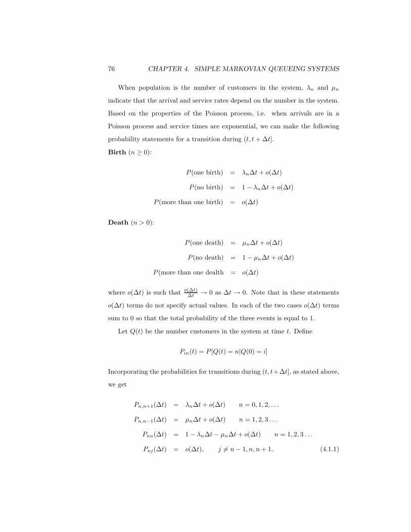
When population is the number of customers in the system, λn and µn
indicate that the arrival and service rates depend on the number in the system.
Based on the properties of the Poisson process, i.e. when arrivals are in a
Poisson process and service times are exponential, we can make the following
probability statements for a transition during (t, t + ∆t].
Birth (n ≥ 0):
P (one birth) = λn∆t + o(∆t)
P (no birth) = 1 − λn∆t + o(∆t)
P (more than one birth) = o(∆t)
Death (n > 0):
P (one death) = µn∆t + o(∆t)
P (no death) = 1 − µn∆t + o(∆t)
P (more than one dealth = o(∆t)
where o(∆t) is such that o(∆t)∆t → 0 as ∆t → 0. Note that in these statements
o(∆t) terms do not specify actual values. In each of the two cases o(∆t) terms
sum to 0 so that the total probability of the three events is equal to 1.
Let Q(t) be the number customers in the system at time t. Define
Pin(t) = P [Q(t) = n|Q(0) = i]
Incorporating the probabilities for transitions during (t, t+∆t], as stated above,
we get
Pn,n+1(∆t) = λn∆t + o(∆t) n = 0, 1, 2, . . .
Pn,n−1(∆t) = µn∆t + o(∆t) n = 1, 2, 3 . . .
Pnn(∆t) = 1 − λn∆t − µn∆t + o(∆t) n = 1, 2, 3 . . .
Pnj(∆t) = o(∆t), j 6= n − 1, n, n + 1. (4.1.1)

4.1. A GENERAL BIRTH AND DEATH QUEUEING MODEL 77
In deriving terms on the right hand side of these equations we have made use
of the simplification of the type
[λn∆t + o(∆t)][1 − µn∆t + o(∆t)] = λn∆t + o(∆t)
[1 − λn∆t + o(∆t)][1 − µn∆t + o(∆t)] = 1 − λn∆t − µn∆t + o(∆t).
The infinitesimal transition rates of (4.1.1) lead to the following generator matrix
for the birth and death process model of the queueing system.
A =
−λ0 λ0
µ1 −(λ1 + µ1) λ1
µ2 −(λ2 + µ2) λ2
·
·
·
(4.1.2)
The generator matrix A of (4.1.2) leads to the following forward Kolmogorov
equations for Pin(t). (For ease of notation, from here onwards, we write Pin(t) ≡
Pn(t) and insert the initial state i only when needed.)
P ′0(t) = −λ0P0(t) + µ1P1(t)
P ′n(t) = −(λn + µn)Pn(t) + λn−1Pn−1(t)
+µn+1Pn+1(t) n = 1, 2, . . . (4.1.3)
As a point of digression, we may note that (4.1.3) can also be derived directly
using (4.1.1) without going through the generator matrix as illustrated below.
Considering the transitions of the process Q(t) during (t, t + ∆t], we have
P0(t + ∆t) = P0(t)[1 − λ0∆t + o(∆t)] + P1(t)[µ, ∆t + o(∆t)]
Pn(t + ∆t) = Pn(t)[1 − λn∆t − µn∆t + o(∆t)]
+Pn−1(t)[λn−1∆t + o(∆t)]

78 CHAPTER 4. SIMPLE MARKOVIAN QUEUEING SYSTEMS
+Pn+1(t)[λn+1∆t + o(∆t)]
+o(∆t) n = 1, 2, . . . (4.1.4)
Subtracting Pn(t) (n = 0, 1, 2 . . .) from both sides of the appropriate equation
in (4.1.4) and dividing by ∆t we get
P0(t + ∆t) − P0(t)∆t
= −λ0P0(t) + µ1P1(t) + o(∆t)
Pn(t + ∆t) − Pn(t)∆t
= −(λn + µn)Pn(t) +o(∆t)∆t
+λn−1Pn−1(t) + µn+1Pn+1(t)
+o(∆t)∆t
Now (4.1.3) follows by letting ∆t → 0.
To determine Pn(t) [≡ Pin(t)], equations (4.1.3) should be solved along with
the initial condition Pi(0) = 1, Pn(0) = 0 for n 6= i. Unfortunately even in
simple cases such as λn = λ and µn = µ, n = 0, 1, 2, 3 . . ., that is when the
arrivals are Poisson and service times are exponential (M/M/1 queue) deriving
Pn(t) is an arduous process. Furthermore in most of the applications the need
for knowing the time dependent behavior is not all that critical. The most
widely used result, therefore, is the limiting result, determined from (4.1.3) by
letting t → ∞.
A general result on Markov processes is given below.
Theorem 4.1.1 (1) If the Markov process is irreducible (all states communi-
cate), then the limiting distribution limt→∞Pn(t) = pn exists and is independent
of the initial conditions of the process. The limits {pn, nεS} are such that they
either vanish identically (i.e. pn = 0 for all nεS) or are all positive and form a
probability distribution (i.e. pn > 0 for all nεS,∑
nεS pn = 1).
(2) The limiting distribution {pn, nεS} of an irreducible recurrent Markov
process is given by the unique solution of the equation pA = 0 and∑
jεS pj = 1,
where p = (p0, p1, p2, . . .).
4.1. A GENERAL BIRTH AND DEATH QUEUEING MODEL 79
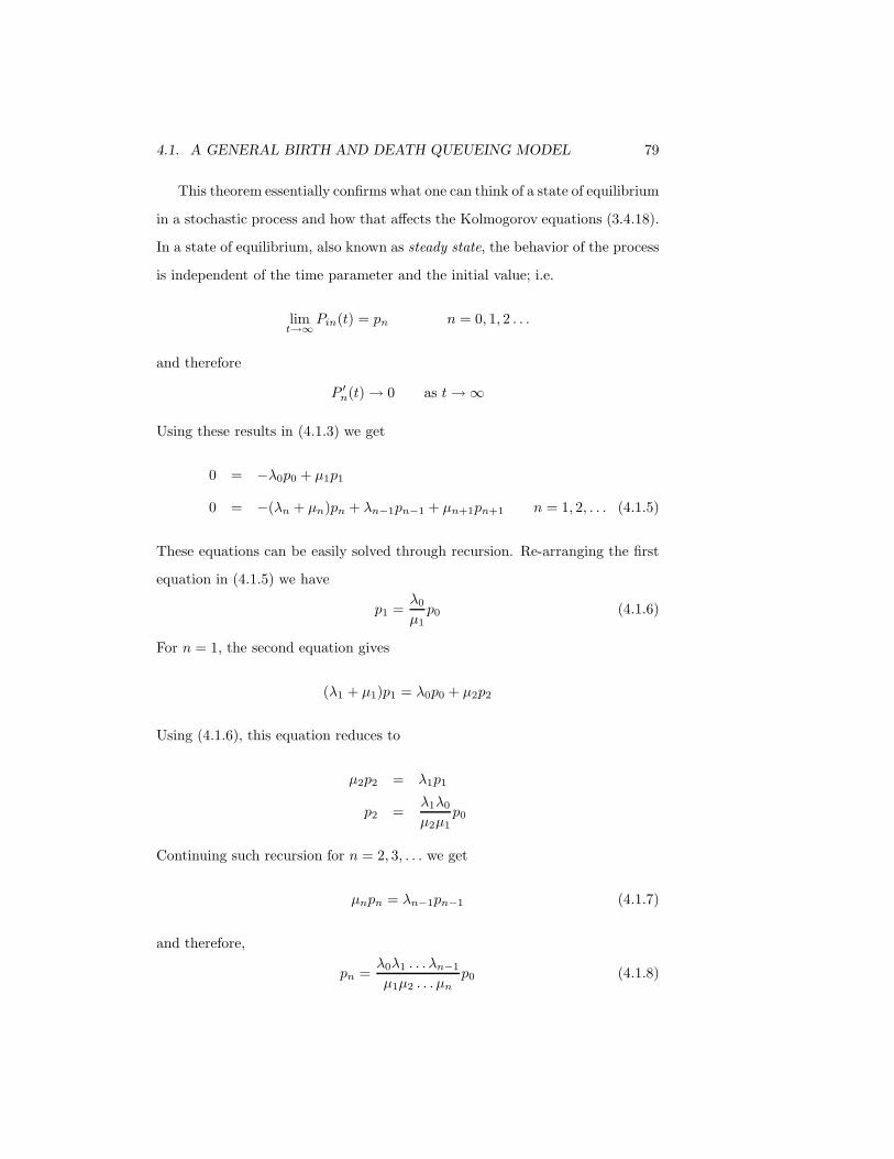
This theorem essentially confirms what one can think of a state of equilibrium
in a stochastic process and how that affects the Kolmogorov equations (3.4.18).
In a state of equilibrium, also known as steady state, the behavior of the process
is independent of the time parameter and the initial value; i.e.
limt→∞
Pin(t) = pn n = 0, 1, 2 . . .
and therefore
P ′n(t) → 0 as t → ∞
Using these results in (4.1.3) we get
0 = −λ0p0 + µ1p1
0 = −(λn + µn)pn + λn−1pn−1 + µn+1pn+1 n = 1, 2, . . . (4.1.5)
These equations can be easily solved through recursion. Re-arranging the first
equation in (4.1.5) we have
p1 =λ0
µ1p0 (4.1.6)
For n = 1, the second equation gives
(λ1 + µ1)p1 = λ0p0 + µ2p2
Using (4.1.6), this equation reduces to
µ2p2 = λ1p1
p2 =λ1λ0
µ2µ1p0
Continuing such recursion for n = 2, 3, . . . we get
µnpn = λn−1pn−1 (4.1.7)
and therefore,
pn =λ0λ1 . . . λn−1
µ1µ2 . . . µnp0 (4.1.8)

80 CHAPTER 4. SIMPLE MARKOVIAN QUEUEING SYSTEMS
Theorem 4.1.1 also gives the normalizing condition∑
nεS pn = 1, which when
applied to (4.1.8), gives
p0 =
[1 +
∞∑
n=1
λ0λ1 . . . λn−1
µ1µ2 . . . µn
]−1
(4.1.9)
The limiting distribution of the state of the birth and death queueing model
is {pn, n = 0, 1, n, . . .} as given by (4.1.8) and (4.1.9). It should be noted that
{pn, n = 0, 1, 2, . . .} are nonzero only when
1 +∞∑
n=1
λ0λ1 . . . λn−1
µ1µ2 . . . µn< ∞ (4.1.10)
In order to derive (4.1.5) deriving (4.1.3) first is not necessary. As noted in
Theorem 4.1, with p = (p0, p1, p2, . . .) and the generator matrix A, (4.1.5) can
be directly obtained from
pA = 0 (4.1.11)
and∞∑
n=1
pn = 1
For the birth and death queueing model the generator matrix A is given by
(4.1.2).
Another way of looking at (4.1.5) is to consider them as representing a
condition of balance among the states. Rearranging (4.1.5)
λ0p0 = µ1p1
(λn + µn)pn = λn−1pn−1 + µn+1pn+1 (4.1.12)
The transitions among the states can be pictorially represented as in Figure
4.1.1.
Figure 4.1.1 (Transition diagram)

4.1. A GENERAL BIRTH AND DEATH QUEUEING MODEL 81
Noting that the λ’s and µ’s represent infinitesimal transition rates in and
out of the states, the equalities in (4.1.12) can be interpreted as (long term
probability of being in state n) × (transition rates out of state n =∑
i=n−1,n+1
(long term probability of being in state i) × (transition rate from state i to
state n).
Such state balance equations can be easily written down using the transition
diagram 4.1.1.
Given above are three ways of writing down the state balance equations:
(1) taking the appropriate limits as t → ∞ in the forward Kolmogorov equa-
tions;
(2) using the equation pA = 0; and
(3) with the help of the transition diagram.
But when using the last method care should be taken to ensure that all
transition have been accounted for. Also in applications the readers may use
any method with which they are comfortable. In our discussion of special models
we normally use the second method based on the generator matrix unless the
transition diagram throws more light on the behavior of the system.
There are two other theorems which establish some important properties of
the limiting distribution of a Markov process with an irreducible state space.
The first of them addresses the concept of stationarity.
Theorem 4.1.2 The limiting distribution of a positive recurrent irreducible
Markov process is also stationary.
A process is said to be stationary if the state distribution is independent of
time, i.e, if
Pn(0) = pn n = 0, 1, 2, . . .
then
Pn(t) = pn for all t.

82 CHAPTER 4. SIMPLE MARKOVIAN QUEUEING SYSTEMS
Since we deal with transition distributions conditional on the initial state in
stochastic processes, the stationarity means that if we use the stationary distri-
bution as the initial state distribution, from then on all time dependent distri-
butions will be the same as the one we started with.
The second theorem enables us to interpret the limiting probability pn, n =
0, 1, 2, . . . as the fraction of time the process occupies state n in the long run.
Theorem 4.1.3 Having started from state i, let Nij(t) be the time spent by the
Markov process in state j during (0, t]. Then
limt→∞
[∣∣∣∣Nij(t)
t− pj
∣∣∣∣ > ε
]= 0.
The general birth and death queueing model encompasses a wide array of special
cases. Some of the widely used models are discussed in the following sections.
4.2 The queue M/M/1
The M/M/1 queue is the simplest of the queueing models used in practice. The
arrivals are assumed to occur in a Poisson process with rate λ. This means that
the number of customers N(t) arriving during a time interval (0, t] has a Poisson
distribution
P [N(t) = j] = e−λt (λt)j!
j = 0, 1, 2 . . .
It also means that the inter-arrival times have an exponential distribution with
probability density
a(x) = λe−λt x > 0
We assume that the service times have an exponential distribution with proba-
bility density
b(x) = µe−µx x > 0
With these assumptions we have
E[interarrival time] =1λ
=1
arrival rate
4.2. THE QUEUE M/M/1 83
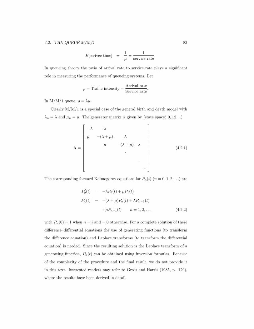
E[serivce time] =1µ
=1
service rate
In queueing theory the ratio of arrival rate to service rate plays a significant
role in measuring the performance of queueing systems. Let
ρ = Traffic intensity =Arrival rateService rate
.
In M/M/1 queue, ρ = λµ.
Clearly M/M/1 is a special case of the general birth and death model with
λn = λ and µn = µ. The generator matrix is given by (state space: 0,1,2,...)
A =
−λ λ
µ −(λ + µ) λ
µ −(λ + µ) λ
·
·
·
(4.2.1)
The corresponding forward Kolmogorov equations for Pn(t) (n = 0, 1, 2, . . .) are
P ′0(t) = −λP0(t) + µP1(t)
P ′n(t) = −(λ + µ)Pn(t) + λPn−1(t)
+µPn+1(t) n = 1, 2, . . . (4.2.2)
with Pn(0) = 1 when n = i and = 0 otherwise. For a complete solution of these
difference–differential equations the use of generating functions (to transform
the difference equation) and Laplace transforms (to transform the differential
equation) is needed. Since the resulting solution is the Laplace transform of a
generating function, Pn(t) can be obtained using inversion formulas. Because
of the complexity of the procedure and the final result, we do not provide it
in this text. Interested readers may refer to Gross and Harris (1985, p. 129),
where the results have been derived in detail.

84 CHAPTER 4. SIMPLE MARKOVIAN QUEUEING SYSTEMS
Limiting distribution
For the limiting probabilities limt→∞Pn(t) = pn, we have the state balance
equations [see (4.1.12)],
λp0 = µp1
(λ + µ)pn = λpn−1 + µpn+1 n = 1, 2, 3 . . . (4.2.3)
Solving these equations along with∑∞
0 pn = 1 (or specializing (4.1.8) and
(4.1.9)) we get
pn = (1 − ρ)ρn n = 0, 1, 2, . . . (4.2.4)
where ρ = λ/µ < 1.
The probability that the server is busy is a performance measure for the
system. Clearly, this utilization factor = 1 − p0 = ρ = traffic intensity in this
case. Recall that we have defined Q(t) as the number of customers in the system.
Write Q(∞) = Q and let Qq be the number in the queue, excluding the one
in service. Now we may define two mean values, L = E(Q) and Lq = E(Qq).
From distribution (4.2.4) we get
L =∞∑
n=1
n(1 − p)ρn =ρ
1 − ρ
which can also be written as
=λ
µ − λ. (4.2.5)
For Lq, we get
Lq =∞∑
n=1
(n − 1)pn
=∞∑
n=1
npn −∞∑
n=1
pn
= L − ρ =ρ2
1 − ρ
=λ2
µ(µ − λ)(4.2.6)

4.2. THE QUEUE M/M/1 85
The utilization factor ρ is the probability that the server is busy when the
system is in equilibrium and therefore, it gives the expected number in service.
With this interpretation we can provide the obvious explanation for (4.2.6) as
E (number in system) = E (number waiting) + E (number in service).
From (4.2.4) we obtain the variance of the number of customers in the system
as
V (Q) =ρ
(1 − ρ)2
=λµ
(µ − λ)2(4.2.7)
Customer waiting time
From a customer viewpoint the waiting time spent in queue and in the system
are two characteristics of importance. When the system is in equilibrium, let
Tq and T be the amount of time a customer spends in queue and in the system
respectively. We assume that the system operates according to a ‘first-come,
first-served‘ (FCFS) queue discipline. We note here that as long as the server
remaines busy when there are customers in the system, and once a service starts,
it is given to its completion, the number in the system is not dependent on the
order in which the customers are served. However, for waiting time the order
of service is a critical factor.
With a FCFS queue discipline, the waiting time for service (Tq) of arriving
customer is the amount of time required to serve the customers already in the
system. The total time in system (T ) is Tq + service time. When there are n
customers in the system, since service times are exponential with parameter µ,
the total service time of n customers is Erlang with probability density
fn(x) = e−µx µnxn−1
(n − 1)!(4.2.8)
Let Fq(t) = P (Tq ≤ t), the distribution function of the waiting time Tq. Clearly
Fq(0) = P (Tq = 0) = P (Q = 0) = 1 − ρ. (4.2.9)

86 CHAPTER 4. SIMPLE MARKOVIAN QUEUEING SYSTEMS
Note that because of the memoryless property of the exponential distribution,
the remaining service time of customer in service is also exponential with the
same parameter µ. Writing dFq(t) = P (t < Tq ≤ t + dt), for t > 0, we have
dFq(t) =∞∑
n=1
pne−µt µntn−1
(n − 1)!dt
= (1 − ρ)∞∑
n=1
ρne−µt µntn−1
(n − 1)!dt
which on simplification gives
= λ(1 − ρ)e−µ(1−ρ)tdt (4.2.10)
Because of the discontinuity at 0 in the distribution of Tq, we get
Fq(t) = P (Tq = 0) +∫ t
0
dFq(t)dt
= 1 − ρe−µ(1−ρ)t (4.2.11)
where we have combined results from (4.2.9) and (4.2.10).
Let E(Tq) = Wq and E(T ) = W . From (4.2.11) we can easily derive
Wq = E(Tq) =ρ
µ(1 − ρ)=
λ
µ(µ − λ)(4.2.12)
and
V (Tq) =ρ(2 − ρ)
µ2(1 − ρ)2(4.2.13)
Recalling that the total time in the system, T , is the sum of Tq and service time,
we get
W = E[T ] =λ
µ(µ − λ+
1µ
=1
µ − λ(4.2.14)
Comparing result (4.2.14) with (4.2.5), we note the relationship
L = λW (4.2.15)
4.2. THE QUEUE M/M/1 87
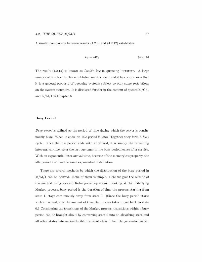
A similar comparison between results (4.2.6) and (4.2.12) establishes
Lq = λWq (4.2.16)
The result (4.2.15) is known as Little’s law in queueing literature. A large
number of articles have been published on this result and it has been shown that
it is a general property of queueing systems subject to only some restrictions
on the system structure. It is discussed further in the context of queues M/G/1
and G/M/1 in Chapter 6.
Busy Period
Busy period is defined as the period of time during which the server is contin-
uously busy. When it ends, an idle period follows. Together they form a busy
cycle. Since the idle period ends with an arrival, it is simply the remaining
inter-arrival time, after the last customer in the busy period leaves after service.
With an exponential inter-arrival time, because of the memoryless property, the
idle period also has the same exponential distribution.
There are several methods by which the distribution of the busy period in
M/M/1 can be derived. None of them is simple. Here we give the outline of
the method using forward Kolmogorov equations. Looking at the underlying
Markov process, busy period is the duration of time the process starting from
state 1, stays continuously away from state 0. (Since the busy period starts
with an arrival, it is the amount of time the process takes to get back to state
0.) Considering the transitions of the Markov process, transitions within a busy
period can be brought about by converting state 0 into an absorbing state and
all other states into an irreducible transient class. Then the generator matrix

88 CHAPTER 4. SIMPLE MARKOVIAN QUEUEING SYSTEMS
(4.2.7) takes the modified form
A =
0 0
µ −(λ + µ) λ
µ −(λ + µ) λ
. . .
(4.2.17)
The corresponding forward Kolmogorov equations for Pn(t) (n = 0, 1, 2, . . .) are
P ′0(t) = µP1(t)
P ′1(t) = −(λ + µ)P1(t) + µP2(t)
P ′n(t) = −(λ + µ)Pn(t) + λPn−1(t) + µPn+1(t)
n = 2, 3, . . . (4.2.18)
With the initial condition P1(0) = 1, Pn(0) = 0 for n 6= 1. Solving these
difference-differential equations require the use of probability generating func-
tions and Laplace transforms. [See, Gross and Harris (1985)].
Let π0(θ) be the Laplace transform of the busy period defined as
π0(θ) =∫ ∞
0
e−θtP ′0(t)dt <(θ) > 0
After appropriate transform operations on (4.2.18) we get
π0(θ) =12λ
[θ + λ + µ −
√(θ + λ + µ)2 − 4λµ
](4.2.19)
This can be inverted to give the explicit form
P ′0(t) = e−(λ+µ)t
√µ/λ
tI1(2
√λµt) (4.2.20)
where Ij(x) is the modified Bessel function defined as
Ij(x) =∞∑
n=0
(x/2)2n+j
n!(n + j)!
Using combinatorial arguments an alternative form for (4.2.20) can be given as
P ′0(t) = e−(λ+µ)t
∞∑
n=1
λn−1µnt2n−2
n!(n − 1)!(4.2.21)

4.2. THE QUEUE M/M/1 89
[See Prabhu (1960)]
Suppose f(x) is the probability density of a random variable X and φ(θ) its
Laplace transform.
φ(θ) =∫ ∞
0
e−θxf(x)dx.
Two easily established properties of φ(θ) are:
E(X) = −φ′(0) (4.2.22)
E(X2) = φ′′(0). (4.2.23)
Let B represent the length of the busy period. Using (4.2.22) and (4.2.23) on
the transform of B given by (4.2.19), we get
E[B] =1
µ − λ(4.2.24)
V [B] =1 + ρ
µ2(1 − ρ)3(4.2.25)
There may be occasions when a busy period starts out with an initial number
of i customers in the system. Because of the Markovian properties of the arrival
process we can show that the transition of the underlying Markov process from i
to 0 can be considered to have made up of i intervals with the same distribution
representing the transitions from i → i − 1, i − 1 → i − 2, . . . , 1 → 0. These i
independent busy periods start with 1 customer in the system. Then if Bi is
the random variable representing a busy period initiated by i customers, we get
E[Bi] =i
µ − λ(4.2.26)
V [Bi] =i(1 + ρ)
µ2(1 − ρ)3(4.2.27)
The explicit expression of the distribution of Bi can be given as
P ′0(t) = e−λ+µ)t i
√µ/λ
tIi(2
√λµt) (4.2.28)
It is easy to visualize the effect of the increase in traffic intensity ρ in the
range (0,1) on the length of the busy period. As ρ increases the length of the

90 CHAPTER 4. SIMPLE MARKOVIAN QUEUEING SYSTEMS
busy period should increase. This can be shown with the help of the Laplace
transform (4.2.19). Consider
limθ→0
π0(θ) = limθ→0
(θ + λ + µ) − [(θ + λ + µ)2 − 4λµ]1/2
2λ
=12λ
[λ + µ −
√(λ − µ)2
]
=
12λ [λ + µ − (µ − λ] if µ ≥ λ
12λ [λ + µ − (λ − µ)] if µ < λ
=
1 if µ > λ
µλ µ < λ
(4.2.29)
But limθ→0 π0(θ) =∫ ∞0
P ′0(t)dt where P ′
0(t) is the probability density of the busy
period distribution. The conclusion we can derive from (4.2.29) is, therefore,
that the busy period has a proper distribution when ρ ≤ 1 and an improper
distribution when ρ > 1. In the latter case, the probability that it will not
terminate is given by 1 − ρ−1.
4.2.1 Departure process
The departure process is the product of processes of arrival and service. When
the server is continuously busy it coincides with the service process. But when
idle times intervene there is a pause in the departures as well. Nevertheless in
equilibrium we can derive properties of the process without reference to arrivals
and service.
Let t1, t2, . . . be the epochs of departure from the system, and define Tn =
tn+1 − tn. When the queue is in equilibrium, i.e., when traffic intensity ρ < 1,
denote this random variable by T . Let Q(x) be the number of customers in the
system,= x amount of time after departure and define
Fn(x) = P [Q(x) = n, T > x] (4.2.30)

4.2. THE QUEUE M/M/1 91
We should note here, as we shall see in Chapter 5, in the M/M/1 queue, the
limiting distribution of the process Q(t) derived in (4.2.4) remains the same
when t in Q(t) is an arbitrary time point, an arrival point or a departure point.
[See, Wolff (1982)]. Therefore, regardless the value of x, we have
P [Q(x) = n] = (1 − ρ)ρn n = 0, 1, 2 . . . (x ≥ 0)
From (4.2.30), we can determine F (x) as
F (x) = P (T > x) =∞∑
0
Fn(x) (4.2.31)
For a specified n, because of the Markovian property of the underlying process,
the random variable T is dependent only on n, not on the preceeding inter-
departure intervals. To establish the relationship between Q(x) and T and to
derive the distribution of T , we start by considering the transition in the interval
(x, x+∆x]. In (4.2.31), F (x) is the probability that T , the time interval between
epochs of the last departure and the next departure, is greater than x. This
means we have to consider the possibility of only arrivals during (x, x + ∆x).
We have
F0(x + ∆x) = F0(x) [1 − λ∆x] + o(∆x)
Fn(x + ∆x) = Fn(x) [1 − λ∆x − µ∆x]
+Fn−1(x)λ∆x + o(∆x) n = 1, 2, . . . (4.2.32)
Rearranging terms in (4.2.32), dividing by ∆x, and letting ∆x → 0, we get
F ′0(x) = −λF0(x)
F ′n(x) = −(λ + µ)Fn(x) + λFn−1(x) n = 1, 2, . . . (4.2.33)
From (4.2.30), we also have
Fn(0) = P [Q(0) = n] = pn (4.2.34)
The first equation in (4.2.33) can be solved by noting
d
dxln F0(x) =
F ′0(x)
F0(x)= −λ.

92 CHAPTER 4. SIMPLE MARKOVIAN QUEUEING SYSTEMS
Hence
ln F0(x) = −λx + C
Now using the initial condition (4.2.23) to determine C we get
F0(x) = p0e−λx (4.2.35)
The general solution to equations (4.2.33) can be obtained by induction. For,
let
Fn−1(x) = pn−1e−λx n = 1, 2, . . .
Substituting this in the second equation of (4.2.33) we get
F ′n(x) + (λ + µ)Fn(x) = λpn−1e
−λx
The general form is now confirmed by multiplying both sides by e(λ+µ)x, inte-
grating and using the initial condition from (4.2.23). We get
Fn(x) = pne−λx n = 1, 2, 3, . . . (4.2.36)
Thus we get
F (x) =∞∑
n=0
pne−λx
= e−λx (4.2.37)
which is the same as the distribution of the interarrival times. Since {pn} is
also the distribution of the number of customers in the system at departure
points, equation (4.3.36) also confirms the independence of the distribution of
T from the queue length distribution at departure points. Note that, here we
are talking about the independence of distribution of two random variables
and not any relationship between their specific values. For a more exhaustive
treatment of this problem see Burke (1956) who has considered this problem for
the multi-server M/M/s queue.
The important result coming out of this analysis states that the departure
process of the M/M/1 queue in equilibrium is the same Poisson as the arrival

4.2. THE QUEUE M/M/1 93
process. Consequently, the expected number of customers served during a length
of time t when the system is in equilibrium is given by λt.
Example 4.2.1
An airport has a single runway. Airplanes have been found to arrive at the rate
of 15 per hour. It is estimated that each landing takes 3 minutes. Assuming a
Poisson process for arrivals and an exponential distribution for landing times,
use an M/M/1 model to determine the following performance measures.
a. Runway utilization. Arrival rate = 15/hr (λ)
Service rate = 60/3/hr = 20/ hr (µ)
Utilization = ρ = λµ = 3
4 .
Ans.
b. Expected number of airplanes waiting to land:
Lq =ρ2
1 − ρ=
(.75)2
.25= 2.25
Ans.
c. Expected waiting time:
E(Wq) =λ
µ(µ − λ)=
1520(20− 15)
=320
hr = 9 mins. Ans .
d. Probability that the waiting will be more than 5 mins? 10 mins? No
waiting?
P (no waiting) = P (Tq = 0) = 1 − ρ = .25 Ans.
P (Tq > t) = ρe−µ(1−ρ)t
P (Tq > 5min) =34e−20(1− 3
4 )5/60
=34e−
2560 = 0.4944 Ans.
P (Tq > 10mins) =34e−
5060 = 0.3259 Ans.
e. Expected number of landings in a 20 minute period = 1560×20 = 5. Ans.

94 CHAPTER 4. SIMPLE MARKOVIAN QUEUEING SYSTEMS
4.3 The queue M/M/s
The multiserver queue M/M/s is the model used most in analyzing service
stations with more than one server such as banks, checkout counters in stores,
checkin counters in airports and the like. The arrival of customers is assumed
to follow a Poisson process, service times are assumed to have an exponential
distribution and let the number of servers be s providing service independently
of each other. We also assume that the arriving customers form a single queue
and the one at the head of the waiting line gets into service as soon as a server
is free. No server stays idle as long as there are customers to serve.
Let λ be the arrival rate and µ the service rate. (This means that the
interarrival times and service times have exponential distributions with densities
λe−λx (x > 0) and µe−µx (x > 0) respectively). Note that the service rate µ is
the same for all servers. In order to use the birth and death model introduced
earlier, we have to establish values for λn and µn, when there are n customers
in the system. Clearly, the arrival rate does not change with the number of
customers in the system (i.e., λ is the constant arrival rate). What about µn
and how does it change?
Suppose n (n = 1, 2, . . . , s) servers are busy at time t. Then, during (t, t+∆t],
the event that a busy server will complete service has the probability µ∆t +
o(∆t). Since there are n busy servers at t, the probability that any one of the
n busy servers will complete service during (t, t + ∆t] can be determined using
the binomial probability distribution as
=(
n
1
)[µ∆t + o(∆t)] [1 − µ∆t + o(∆t)]n−1
= nµ∆t + o(∆t) (4.3.1)
Note that o(∆t)∆t → 0 as ∆t → 0.
In a similar manner the probability that a number r(> 1) of the busy server

4.3. THE QUEUE M/M/S 95
will complete service during (t, t + ∆t] can be given as
=(
n
r
)[µ∆t + o(∆t)]r [1 − µ∆t + o(∆t)]n−r
= o(∆t)
Therefore when there are n busy servers at time t, the only event in [t, t +
∆t] contributing to the reduction in that number that has a non-negligible
probability, is the completion of one service, and it has the probability given in
(4.3.1). Hence the service rate at that time is nµ. Then in the framework of
the birth and death queueing model, we have
λn = λ n = 0, 1, 2, . . .
µn = nµ n = 1, 2, . . . , s − 1
= sµ n = s, s + 1, . . . (4.3.2)
The generator matrix A for the process can be given as
A =
0 −λ λ
1 µ −(λ + µ) λ
2 2µ −(λ + 2µ) λ... · ·
s sµ −(λ + sµ) λ
s + 1 sµ −(λ + sµ) λ...
. . .
(4.3.3)
Let Q(t) be the number of customers in the system at time t and Pn(t) =
P [Q(t) = n|Q(0) = i]. Forward Kolmogorov equations for Pn(t) can be written
down specializing (4.1.3). Since solving such equations is very cumbersome we
do not plan to attempt it here. Interested readers may refer to Saaty (1961).
96 CHAPTER 4. SIMPLE MARKOVIAN QUEUEING SYSTEMS
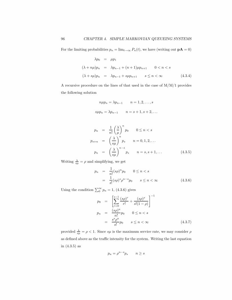
For the limiting probabilities pn = limt→∞ Pn(t), we have (writing out pA = 0)
λp0 = µp1
(λ + nµ)pn = λpn−1 + (n + 1)µpn+1 0 < n < s
(λ + sµ)pn = λpn−1 + sµpn+1 s ≤ n < ∞ (4.3.4)
A recursive procedure on the lines of that used in the case of M/M/1 provides
the following solution
nµpn = λpn−1 n = 1, 2, . . . , s
sµpn = λpn−1 n = s + 1, s + 2, . . .
[Also see (4.1.7)]. Therefore
pn =1n!
(λ
µ
)n
p0 0 ≤ n < s
ps+n =(
λ
sµ
)n
ps n = 0, 1, 2, . . .
pn =(
λ
sµ
)n−s
ps n = s, s + 1, . . . (4.3.5)
Writing λsµ = ρ and simplifying, we get
pn =1n!
(sρ)np0 0 ≤ n < s
=1s!
(sρ)sρn−sp0 s ≤ n < ∞ (4.3.6)
Using the condition∑∞
0 pn = 1, (4.3.6) gives
p0 =
[s−1∑
r=0
(sρ)r
r!+
(sρ)s
s!(1 − ρ)
]−1
pn =(sρ)n
n!p0 0 ≤ n < s
=ssρn
s!p0 s ≤ n < ∞ (4.3.7)
provided λsµ = ρ < 1. Since sµ is the maximum service rate, we may consider ρ
as defined above as the traffic intensity for the system. Writing the last equation
in (4.3.5) as
pn = ρn−sps n ≥ s

4.3. THE QUEUE M/M/S 97
we may say that when the number of customers in the system is ≥ s, the system
behaves like an M/M/1 with service rate sµ. For convenience we may also write
α = λµ , so that α/s = ρ. An alternative form of (4.3.7) using α, can be given as
p0 =
[s−1∑
r=0
αr
r!+
αs
s!(1 − α/s)−1
]−1
pn =αn
n!p0 0 ≤ n < s
=αs
s!(α
s)n−sp0 s ≤ n < ∞ (4.3.8)
It should be noted that customers will have to wait for service only if the number
in the system is ≥ s. The probability of this event is given by∑∞
n=s pn and
hence
P (customer delay) = C(s, α)
=αs
s!
(1 − α
s
)−1[
s−1∑
r=0
αr
s!
(1 − α
s
)−1]−1
(4.3.9)
(4.3.10)
The formula for C(s, α) is known in the literature as Erlang’s Delay Formula or
Erlang’s Second Formula and it is also denoted as E2,s(α). [This result was first
published by Erlang in 1917.] Before the advent of computers, the telephone
industry used C(s, α) graphs plotted for different combinations of s and α.
Writing L and Lq as the mean number of customers in the system and
the number in the queue respectively we may derive them as follows. Using
expressions from (4.3.7) we get (writing sρ = α when convenient)
∞∑
n=1
npn = p0
[s∑
n=1
nαn
n!+
∞∑
n=s+1
nρn−s αs
s!
]
= p0
[α
s−1∑
n=1
αn−1
(n − 1)!+
αs
s!
∞∑
n−s=1
nρn−s
]
= p0
[α
s−1∑
r=0
αr
r!+
αs
s!
∞∑
r=1
(r + s)ρr
]
98 CHAPTER 4. SIMPLE MARKOVIAN QUEUEING SYSTEMS
= p0
[α
s−1∑
r=0
αr
r!+
αs
s!
(ρ
(1 − ρ)2+
sρ
(1 − ρ)
)]
=ραsp0
s!(1 − ρ)2+ αp0
[s−1∑
r=0
αr
r!+
αs
s!(1 − ρ)
]
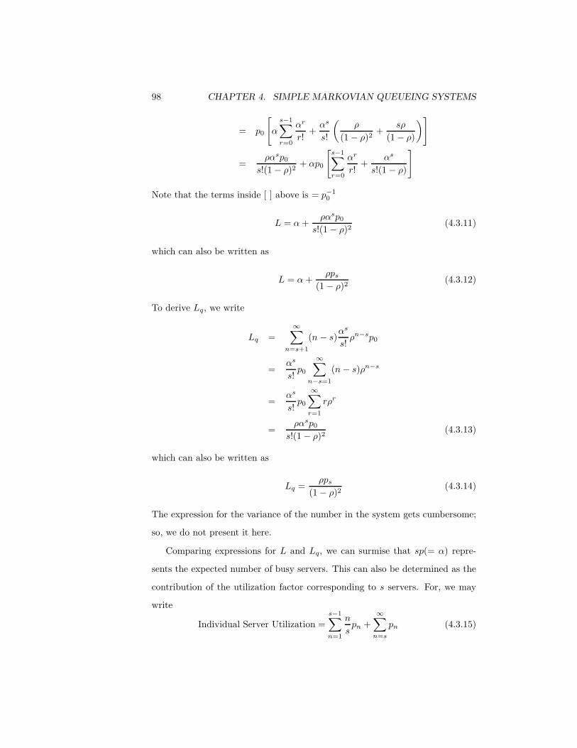
Note that the terms inside [ ] above is = p−10 . [See (4.3.7).] Thus we get
L = α +ραsp0
s!(1 − ρ)2(4.3.11)
which can also be written as
L = α +ρps
(1 − ρ)2(4.3.12)
To derive Lq, we write
Lq =∞∑
n=s+1
(n − s)αs
s!ρn−sp0
=αs
s!p0
∞∑
n−s=1
(n − s)ρn−s
=αs
s!p0
∞∑
r=1
rρr
=ραsp0
s!(1 − ρ)2(4.3.13)
which can also be written as
Lq =ρps
(1 − ρ)2(4.3.14)
The expression for the variance of the number in the system gets cumbersome;
so, we do not present it here.
Comparing expressions for L and Lq, we can surmise that sp(= α) repre-
sents the expected number of busy servers. This can also be determined as the
contribution of the utilization factor corresponding to s servers. For, we may
write
Individual Server Utilization =s−1∑
n=1
n
spn +
∞∑
n=s
pn (4.3.15)
4.3. THE QUEUE M/M/S 99
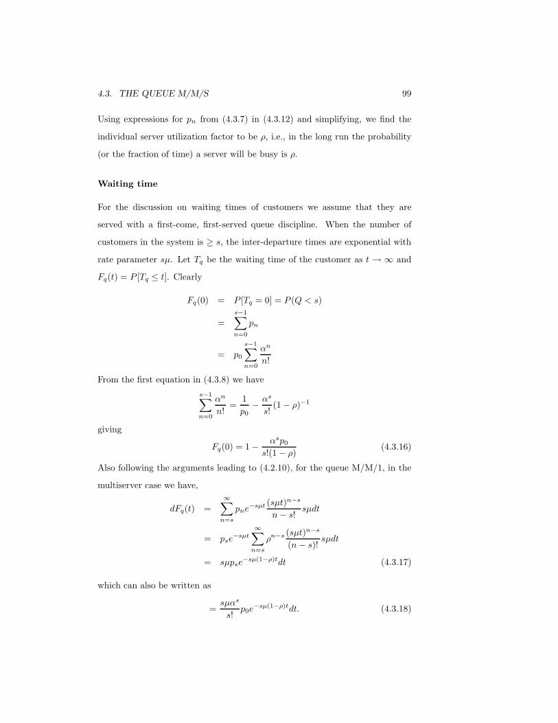
Using expressions for pn from (4.3.7) in (4.3.12) and simplifying, we find the
individual server utilization factor to be ρ, i.e., in the long run the probability
(or the fraction of time) a server will be busy is ρ.
Waiting time
For the discussion on waiting times of customers we assume that they are
served with a first-come, first-served queue discipline. When the number of
customers in the system is ≥ s, the inter-departure times are exponential with
rate parameter sµ. Let Tq be the waiting time of the customer as t → ∞ and
Fq(t) = P [Tq ≤ t]. Clearly
Fq(0) = P [Tq = 0] = P (Q < s)
=s−1∑
n=0
pn
= p0
s−1∑
n=0
αn
n!
From the first equation in (4.3.8) we have
s−1∑
n=0
αn
n!=
1p0
− αs
s!(1 − ρ)−1
giving
Fq(0) = 1 − αsp0
s!(1 − ρ)(4.3.16)
Also following the arguments leading to (4.2.10), for the queue M/M/1, in the
multiserver case we have,
dFq(t) =∞∑
n=s
pne−sµt (sµt)n−s
n − s!sµdt
= pse−sµt
∞∑
n=s
ρn−s (sµt)n−s
(n − s)!sµdt
= sµpse−sµ(1−ρ)tdt (4.3.17)
which can also be written as
=sµαs
s!p0e
−sµ(1−ρ)tdt. (4.3.18)
100 CHAPTER 4. SIMPLE MARKOVIAN QUEUEING SYSTEMS
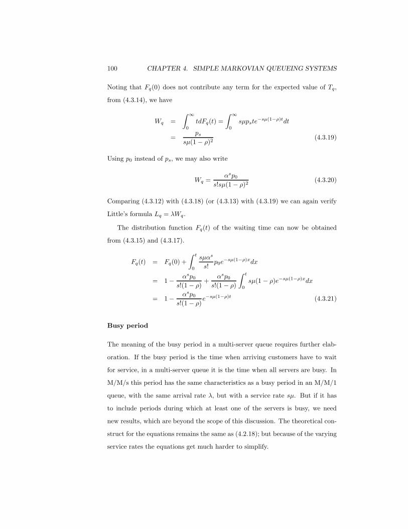
Noting that Fq(0) does not contribute any term for the expected value of Tq,
from (4.3.14), we have
Wq =∫ ∞
0
tdFq(t) =∫ ∞
0
sµpste−sµ(1−ρ)tdt
=ps
sµ(1 − ρ)2(4.3.19)
Using p0 instead of ps, we may also write
Wq =αsp0
s!sµ(1 − ρ)2(4.3.20)
Comparing (4.3.12) with (4.3.18) (or (4.3.13) with (4.3.19) we can again verify
Little’s formula Lq = λWq .
The distribution function Fq(t) of the waiting time can now be obtained
from (4.3.15) and (4.3.17).
Fq(t) = Fq(0) +∫ t
0
sµαs
s!p0e
−sµ(1−ρ)xdx
= 1 − αsp0
s!(1 − ρ)+
αsp0
s!(1 − ρ)
∫ t
0
sµ(1 − ρ)e−sµ(1−ρ)xdx
= 1 − αsp0
s!(1 − ρ)e−sµ(1−ρ)t (4.3.21)
Busy period
The meaning of the busy period in a multi-server queue requires further elab-
oration. If the busy period is the time when arriving customers have to wait
for service, in a multi-server queue it is the time when all servers are busy. In
M/M/s this period has the same characteristics as a busy period in an M/M/1
queue, with the same arrival rate λ, but with a service rate sµ. But if it has
to include periods during which at least one of the servers is busy, we need
new results, which are beyond the scope of this discussion. The theoretical con-
struct for the equations remains the same as (4.2.18); but because of the varying
service rates the equations get much harder to simplify.

4.3. THE QUEUE M/M/S 101
Departure process
As mentioned during the discussion of the departure process of the queue
M/M/1, the procedure outlined there applies to M/M/s as well. In fact, the
differential equations (4.2.33) can be extended to include varying service rates
and the inductive procedure adopted in their solution applies in this case as
well. Using the same notations as before we get
Fn(x) = pne−λx, n = 0, 1, 2, . . .
and
F (x) =∞∑
n=0
pne−λx
= e−λx (4.3.22)
[see Burke (1956) for details. Also Reich (1965)].
Example 4.3.1
In the airport problem of Example 4.2.1, how would the performance measures
change if there are two runways while assuming the same arrival and service
rates?
a. Runway utilization.
Arrival rate = 15/hr (λ)
Service rate = 20/hr (µ)
No. of servers = 2 (s)
Utilization of each runway = ρ = λsµ = 3
8 Ans.
b. Expected number of airplanes waiting to land:
Lq =ραsp0
s!(1 − ρ)2
Note: α = sρ = 34
p0 =
[1∑
r=0
αr
r!+
αs
s!(1 − ρ)
]−1

102 CHAPTER 4. SIMPLE MARKOVIAN QUEUEING SYSTEMS
=[1 +
34
+(3/4)2
2(1 − 3
8)−1
]−1
= 0.4545
Lq =[(38)(
34)2(0.4545)
]/2(
58)2
= 0.1227 Ans.
c. Expected waiting time
Wq =αsp0
s!sµ(1 − ρ)2
=[(34)2(0.4545)
]/2× 2 × 20(1 − 3
8)2
= 0.00818 hrs = 0.49 mins. Ans.
d . Probability that the waiting will be more than 5 mins? 10 mins? no
waiting?
P (no waiting) = Fq(0) = 1 − αsp0
s!(1 − ρ)
= 1 −( 34 )2(0.4545)2(1 − 3/8)
= 0.7955 Ans.
P (Tq > t) =αsp0
s!(1 − ρ)e−sµ(1−ρ)t
P (Tq > 5min) =(3/4)2(0.4545)
2(5/8)e−2( 1
3 )( 58 )5
= 0.1245 Ans.
P (Tq > 10 min) = 0.0155 Ans.
e. Expected number of landings in a 20 minute period = 1560 × 20 = 5. Ans.
[The departure process is Poisson with parameter λ].
Example 4.3.2

4.3. THE QUEUE M/M/S 103
A bank has established two counters one for commercial banking and the second
for personal banking. Arrival and service rates at the commercial counter are
6 and 12 per hours respectively. The corresponding numbers at the personal
banking counter are 12 and 24 respectively. Assume that arrivals occur in
Poisson processes and service times have exponential distributions.
(i) Assuming that the two counters operate independently of each other
determine the expected number of waiting customers and their mean waiting
time at each counter.Commercial Personal
λ 6/hr 12/hr
µ 12/hr 24/hr
ρ = λµ 0.5 0.5
Lq = ρ2
1−ρ 0.5 0.5 Ans.
Wq = ρµ(1−ρ) 5 mins. 2.5 mins. Ans.
(ii) What is the effect of operating the two queues as a two server queue
with arrival rate 18/hr and service rate 18/hr? What conclusion can you drawn
from this operation?
Two-server queue
λ 18/hr
µ 18/hr
Number of servers (s) 2
ρ = λsµ .5
α = λµ 1
p0 = [∑1
0αr
r! + α2
2(1−ρ) ]−1 0.4
Lq = ρα2p02(1−ρ)2 0.4 Ans.
Wq = α2p0(2) 2µ(1−ρ)2 1.33 mins. Ans.
Conclusion: The two-server queue operation is more efficient than the two
single-server operations.

104 CHAPTER 4. SIMPLE MARKOVIAN QUEUEING SYSTEMS
Incidentally, the efficiency of multiserver queues over single server systems
is the reason that multi-server service systems, whenever possible, use single
waiting lines feeding multiple counters for service; e.g. airline checkin counters;
checkout counters in stores effectively operate this way because of jockeying
among the waiting lines.
4.4 The finite queue M/M/s/K.
When the waiting room in a queueing system has a capacity limit we get a finite
queue. In most situations, a finite queue occurs more naturally than a queue
with waiting room of infinite size. However, as the capacity limit gets larger, the
behavior of the system approximates that of an infinite capacity system and in
such cases we are justified in ignoring the size limit. A communication system
with a finite buffer and several service channels is a good example of a finite
queue.
Consider an s-server queueing system with Poisson arrivals, exponential ser-
vice and a capacity limit of K for the number in the system. Clearly K ≥ s.
Assume that λ and µ are the arrival and service rates respectively. These as-
sumptions result in the following infinitesimal transition rates in the generalized
birth and death queueing model.
λn = λ n = 0, 1, 2, . . . , K − 1
µn = nµ n = 1, 2, . . . , s − 1
= sµ n = s, s + 1, . . . , K (4.4.1)
Note that we assume the arrivals to be denied entry to the system (or the arrival
process stops) once the number in the system reaches K. The generator matrix

4.4. THE FINITE QUEUE M/M/S/K. 105
A is essentially the same as (4.3.3), in the first K rows,
A =
0 −λ λ
1 µ −(λ + µ) λ...
. . .
s sµ −(λ + sµ) λ...
. . .
K − 1 sµ −(µ + sµ) λ
K sµ −sµ
(4.4.2)
For the limiting probabilities {pn} n = 0, 1, 2, . . . , K, the state balance equations
can be written down in a manner similar to (4.3.4). The solution corresponding
to (4.3.6) can be given as
pn =1n!
(λ
µ)np0 0 ≤ n ≤ s
=1s!
(λ
µ)s(
λ
sµ)n−sp0 s ≤ n ≤ K
Writing λsµ = ρ and λ
µ = α, p0 can be obtained using the condition∑K
n=0 pn = 1.
p0 =
[s−1∑
r=0
αr
r!+
αs
s!
K∑
n=s
ρn−s
]−1
.
Since the second sum on the right hand side of the expression for p0 is a finite
sum, we need not impose the condition ρ < 1 for a solution with p0 > 0. Thus
we have
p0 =
[s−1∑
r=0
αr
r!+
αs
s!1 − ρK−s+1
1 − ρ
]ρ 6= 1
=
[s−1∑
r=0
αr
r!+
αs
s!(K − s + 1)
]−1
ρ = 1
pn =αn
n!p0 0 ≤ n < s
=αs
s!ρn−sp0 s ≤ n ≤ K (4.4.3)
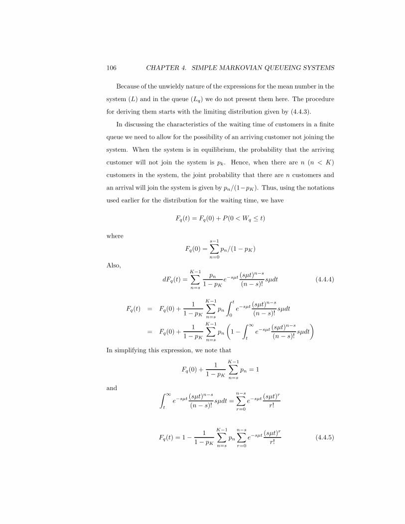
106 CHAPTER 4. SIMPLE MARKOVIAN QUEUEING SYSTEMS
Because of the unwieldy nature of the expressions for the mean number in the
system (L) and in the queue (Lq) we do not present them here. The procedure
for deriving them starts with the limiting distribution given by (4.4.3).
In discussing the characteristics of the waiting time of customers in a finite
queue we need to allow for the possibility of an arriving customer not joining the
system. When the system is in equilibrium, the probability that the arriving
customer will not join the system is pk. Hence, when there are n (n < K)
customers in the system, the joint probability that there are n customers and
an arrival will join the system is given by pn/(1−pK). Thus, using the notations
used earlier for the distribution for the waiting time, we have
Fq(t) = Fq(0) + P (0 < Wq ≤ t)
where
Fq(0) =s−1∑
n=0
pn/(1 − pK)
Also,
dFq(t) =K−1∑
n=s
pn
1− pKe−sµt (sµt)n−s
(n − s)!sµdt (4.4.4)
Fq(t) = Fq(0) +1
1 − pK
K−1∑
n=s
pn
∫ t
0
e−sµt (sµt)n−s
(n − s)!sµdt
= Fq(0) +1
1 − pK
K−1∑
n=s
pn
(1 −
∫ ∞
t
e−sµt (sµt)n−s
(n − s)!sµdt
)
In simplifying this expression, we note that
Fq(0) +1
1 − pK
K−1∑
n=s
pn = 1
and ∫ ∞
t
e−sµt (sµt)n−s
(n − s)!sµdt =
n−s∑
r=0
e−sµt (sµt)r
r!
[See Eq. (2.1.9)]. Then we get
Fq(t) = 1 − 11 − pK
K−1∑
n=s
pn
n−s∑
r=0
e−sµt (sµt)r
r!(4.4.5)

4.4. THE FINITE QUEUE M/M/S/K. 107
Taking expectations, we get
Wq =∫ ∞
0
tdFq(t) =K−1∑
n=s
pn
1 − pK
∫ ∞
0
e−sµt (sµt)n−s
(n − s)!sµtdt
=1
sµ(1 − pK)
K−1∑
n=s
(n − s + 1)pn (4.4.6)
The expected time in the system can be obtained as
W = Wq +1µ
(4.4.7)
The expected number of customers in the queue and in the system are obtained
by noting that the effective arrival rate is λ(1 − pK).
L = λ(1 − pK)W (4.4.8)
Lq = λ(1 − pK)Wq (4.4.9)
Two special cases of this system have been used widely in applications:
(i) M/M/1/K and
(ii) M/M/s/s .
The finite queue M/M/1/K
For single server systems with limited waiting room M/M/1/K is a better model
than the infinite waiting room queue M/M/1. A direct specialization of results
(4.4.3) - (4.4.7) yields the following results. Note that s = 1 and α = ρ = λµ .
p0 =1 − ρ
1 − ρK+1ρ 6= 1
=1
K + 1ρ = 1 (4.4.10)
pn =(1 − ρ)ρn
1 − ρK+1ρ 6= 1
=1
K + 1(4.4.11)
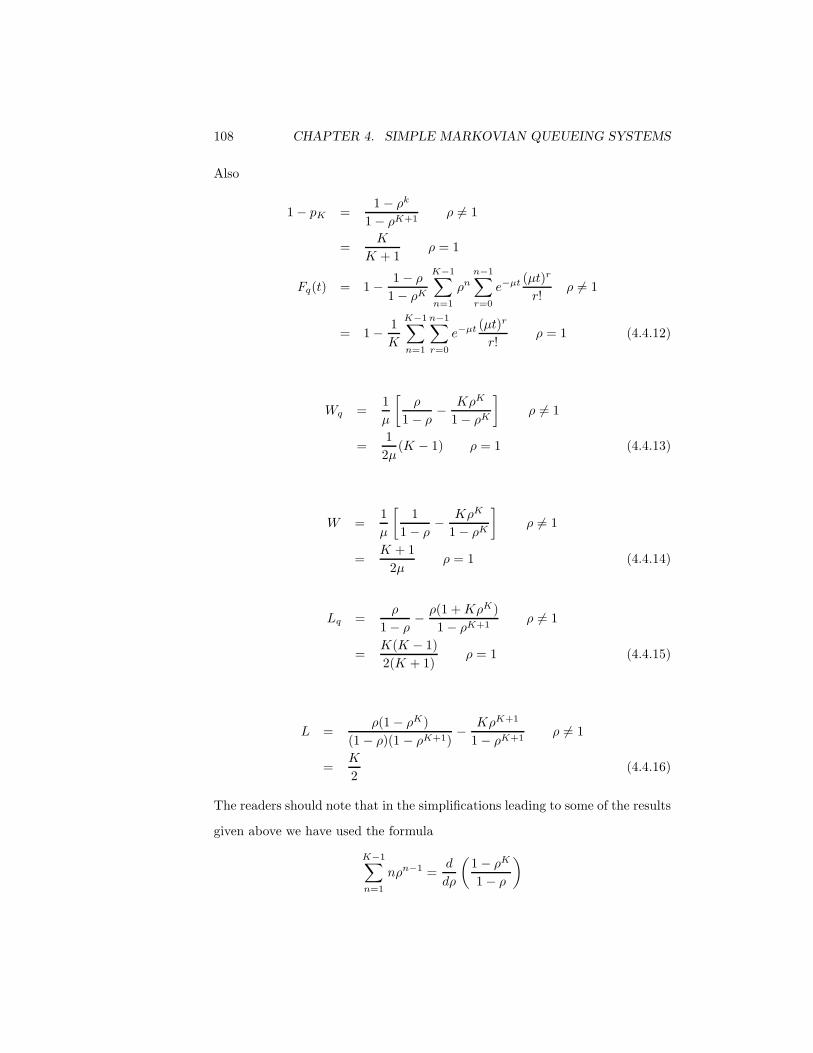
108 CHAPTER 4. SIMPLE MARKOVIAN QUEUEING SYSTEMS
Also
1 − pK =1 − ρk
1 − ρK+1ρ 6= 1
=K
K + 1ρ = 1
Fq(t) = 1 − 1 − ρ
1 − ρK
K−1∑
n=1
ρnn−1∑
r=0
e−µt (µt)r
r!ρ 6= 1
= 1 − 1K
K−1∑
n=1
n−1∑
r=0
e−µt (µt)r
r!ρ = 1 (4.4.12)
Wq =1µ
[ρ
1 − ρ− KρK
1 − ρK
]ρ 6= 1
=12µ
(K − 1) ρ = 1 (4.4.13)
W =1µ
[1
1 − ρ− KρK
1 − ρK
]ρ 6= 1
=K + 1
2µρ = 1 (4.4.14)
Lq =ρ
1 − ρ− ρ(1 + KρK)
1 − ρK+1ρ 6= 1
=K(K − 1)2(K + 1)
ρ = 1 (4.4.15)
L =ρ(1 − ρK)
(1 − ρ)(1 − ρK+1)−
KρK+1
1 − ρK+1ρ 6= 1
=K
2(4.4.16)
The readers should note that in the simplifications leading to some of the results
given above we have used the formula
K−1∑
n=1
nρn−1 =d
dρ
(1 − ρK
1 − ρ
)

4.4. THE FINITE QUEUE M/M/S/K. 109
Example 4.4.1
A small mail order business has one telephone line and a facility for call waiting
for two additional customers. Orders arrive at the rate of one per minute and
each order requires 2 minutes and 30 seconds to take down the particulars.
Model this system as an M/M/1/3 queue and answer the following questions.
(a) What is the expected number of calls waiting in the queue? What is the
mean wait in queue?
Assuming that the arrivals are in a Poisson process with rate 1 per minute
(λ) and the service times are exponential with mean 2.5 mins (1/µ). We
have ρ = 2.5. Also K = 3. Using the first result from (4.4.15) we get
Lq =2.5
1 − 2.5−
(2.5)[1 + 3(2.5)3]1 − (2.5)4
= 1.4778 Ans.
Since λ = 1, the mean waiting time in queue
Wq = 1.4778 mins.
Ans.
(b) What is the probability that the call has to wait for more than 1.5 mins
before getting served?
We use the formula for 1 − Fq(t) from (4.4.12) with t = 1.5, 1/µ = 2.5
and ρ = 2.5. We get,
P(Wait in queue > 1.5 mins)
=1 − 2.5
1 − (2.5)3
3−1∑
n=1
(2.5)nn−1∑
r=0
e−1.52.5
(1.5/2.5)r
r!
= 0.7036 Ans.
(c) Because of the excessive waiting time of customers, the business decides
to use two telephone lines instead of one, keeping the same total capacity
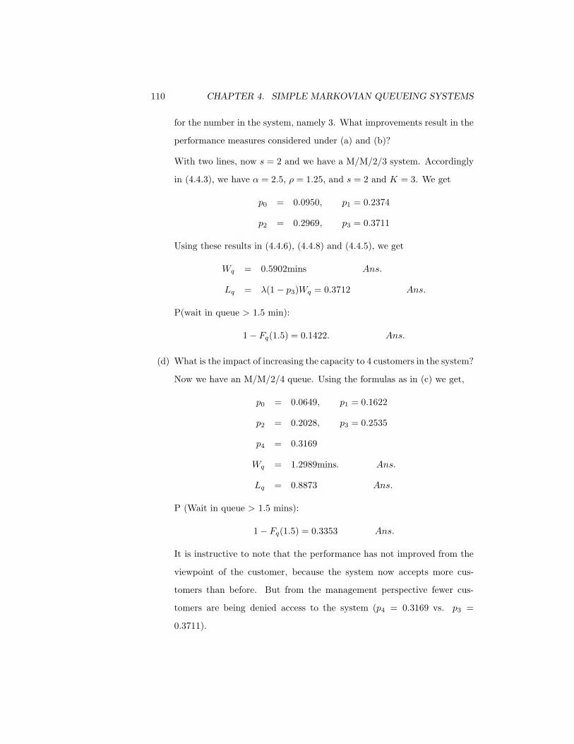
110 CHAPTER 4. SIMPLE MARKOVIAN QUEUEING SYSTEMS
for the number in the system, namely 3. What improvements result in the
performance measures considered under (a) and (b)?
With two lines, now s = 2 and we have a M/M/2/3 system. Accordingly
in (4.4.3), we have α = 2.5, ρ = 1.25, and s = 2 and K = 3. We get
p0 = 0.0950, p1 = 0.2374
p2 = 0.2969, p3 = 0.3711
Using these results in (4.4.6), (4.4.8) and (4.4.5), we get
Wq = 0.5902mins Ans.
Lq = λ(1 − p3)Wq = 0.3712 Ans.
P(wait in queue > 1.5 min):
1 − Fq(1.5) = 0.1422. Ans.
(d) What is the impact of increasing the capacity to 4 customers in the system?
Now we have an M/M/2/4 queue. Using the formulas as in (c) we get,
p0 = 0.0649, p1 = 0.1622
p2 = 0.2028, p3 = 0.2535
p4 = 0.3169
Wq = 1.2989mins. Ans.
Lq = 0.8873 Ans.
P (Wait in queue > 1.5 mins):
1 − Fq(1.5) = 0.3353 Ans.
It is instructive to note that the performance has not improved from the
viewpoint of the customer, because the system now accepts more cus-
tomers than before. But from the management perspective fewer cus-
tomers are being denied access to the system (p4 = 0.3169 vs. p3 =
0.3711).

4.4. THE FINITE QUEUE M/M/S/K. 111
The loss system M/M/s/s
The queue M/M/s/s in which customers arriving when all servers are busy are
not allowed entry to the system is one of the earliest systems considered by
A. K. Erlang (1917). Before the introduction of call waiting buffers, telephone
systems operated strictly as loss systems.
Let customer arrivals be Poisson with parameter λ and service times be
exponential with mean 1/µ. There are s servers and all customers arriving
when all servers are busy are lost to the system. Thus the state space for the
number of customers in the system is {0, 1, 2, . . . , s}. The generator matrix for
the birth and death model is the truncated version of (4.3.3):
A =
0 −λ λ
1 µ −(λ + µ) λ
2 2µ −(λ + 2µ) λ...
...
s − 1 (s − 1)µ −[λ + (s − 1)µ] λ
s sµ −sµ
(4.4.17)
Accordingly the limiting probabilities are obtained using the state balance equa-
tions,
λp0 = µp1
(λ + nµ)pn = λpn−1 + (n + 1)µpn+1 1 ≤ n < s
sµps = λps−1 (4.4.18)
Writing λµ = α, (4.4.18) can be solved re cursively to give
p0 =[1 + α + α2/2! + . . . + αs/s!
]−1
pn =αn
n!p0 n = 0, 1, . . . , s (4.4.19)

112 CHAPTER 4. SIMPLE MARKOVIAN QUEUEING SYSTEMS
This gives
ps =αs
/s!
1 + α + α2
2! + . . . + αs
s!
(4.4.20)
which is the probability that a customer is blocked from entering the system.
(Telephones calls are lost.) Also λps gives the expected number of customers
who will be blocked from entering the system in unit time. Eq. (4.4.20) is
commonly known as Erlang’s Loss Formula or Erlang’s First Formula and de-
noted as E1,s(α) or B(s, α). This formula has been extensively used in designing
telephone systems by traffic engineers.
For ready reference ps values are plotted for different values of s, against
varying values of the offered load α. In the teletraffic literature it is common to
measure the offered load (the ratio of arrival rate to the service rate) in Erlangs
for convenience. It should be noted that in the telephone industry parlance the
carried load is given by α(1−ps), since a proportion ps of the arriving customers
are lost to the system.
The right hand side expression in the formula (4.4.20) has been shown to
be a convex function of s in [0,∞) for α > 0. [See Smith and Whitt (1981)
and Jagers and van Doorn (1986)]. Another characteristic of this formula is its
validity even when service times have a general distribution. We shall discuss
this property further in Chapter 8.
4.5 The infinite server queue M/M/∞
Even though calling a system with an infinite number of servers, consequently
with no waiting line, a misnomer, the system M/M/∞ is being identified as
such because of its structure. The customers arrive in a Poisson process and the
service times have an exponential distribution. Let λ and µ be the arrival and
service rates. We assume that the system is able to provide service as soon as
the customer arrives. A simple example is a large grocery store or a supermarket
4.5. THE INFINITE SERVER QUEUE M/M/∞ 113
where customers serve themselves while picking up merchandise. The checkout
counters will then have to be modeled as an M/M/s system. Another example
is a large parking lot.
When there are n customers in the system the service rate is nµ (n =
1, 2, . . .). For the birth and death parameters or the queueing model, we then
get
λn = λ n = 0, 1, 2, . . .
µn = nµ n = 1, 2, 3 . . . (4.5.1)
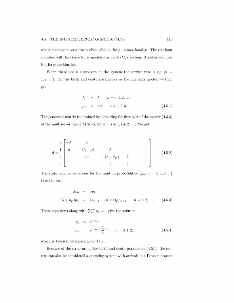
The generator matrix is obtained by extending the first part of the matrix (4.3.3)
of the multiserver queue M/M/s, for n = s + 1, s + 2, . . .. We get
A =
0 −λ λ
1 µ −(λ + µ) λ
2 2µ −(λ + 2µ) λ . . ....
......
(4.5.2)
The state balance equations for the limiting probabilities {pn, n = 0, 1, 2 . . .}
take the form
λp0 = µp1
(λ + nµ)pn = λpn−1 + (n + 1)µpn+1 n = 1, 2, . . . (4.5.3)
These equations along with∑∞
0 pn = 1 give the solution
p0 = e−λ/µ
pn = e−λ/µ(λ
µ)n n = 0, 1, 2, . . . (4.5.4)
which is Poisson with parameter λ/µ.
Because of the structure of the birth and death parameters (4.5.1), the sys-
tem can also be considered a queueing system with arrivals in a Poisson process

114 CHAPTER 4. SIMPLE MARKOVIAN QUEUEING SYSTEMS
and exponential service times in a linearly dependent arrival rate nµ when there
are nµ customers in the system. It should be noted the departure process prop-
erties established in Section 4.2 apply to this system as well and therefore, the
departure process of customers in equilibrium, has the same Poisson distribu-
tion, as the arrival process. This property justifies the use of an M/M/s model
for the checkout counters in the supermarket example cited above.
4.6 Finite source queues
The source of customers is an important element of a queueing system. In
the models discussed so far we have assumed that the source is infinite. This
assumption is essential in characterizing the arrivals to the system as being
Poisson. If the source of customers is finite, a pre-specified number in the
population, even though we cannot assume a Poisson process for arrivals, we
can generate a Markovian arrival process with the following arrival scheme.
Suppose there are M customers in the population. Each customer goes
through two alternating phases, not needing service and in need of service.
An example is a population of machines that require service when they become
inoperative. Another example is a subscriber group in an information exchange.
Assume that the phase during which the customer does not require service is
exponentially distributed with mean 1/λ. This implies that, if at time t, a
customer is in this phase, during (t, t + ∆t], the event that it will need service
has the probability λt + o(∆t). Thus, if there are k customers in that phase
requiring no service at time t, the probability that one of them will call for
service is kλ + o(∆t)] [see discussion preceeding (4.3.1)]. When the service
times are exponential, we are now able to use a birth and death queueing model
for such a system.
For convenience, let use define the state of the process as the number of
customers requiring service. It takes values in S : {0, 1, 2, . . . , M}. Note that if
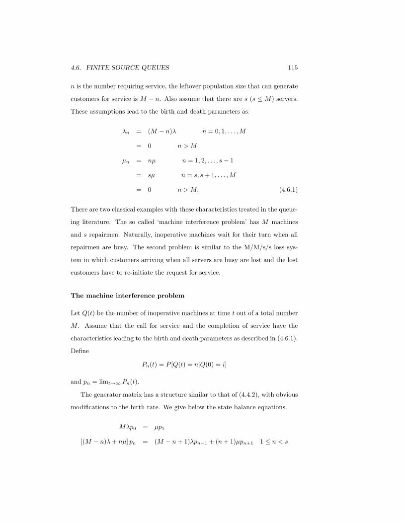
4.6. FINITE SOURCE QUEUES 115
n is the number requiring service, the leftover population size that can generate
customers for service is M − n. Also assume that there are s (s ≤ M) servers.
These assumptions lead to the birth and death parameters as:
λn = (M − n)λ n = 0, 1, . . . , M
= 0 n > M
µn = nµ n = 1, 2, . . . , s − 1
= sµ n = s, s + 1, . . . , M
= 0 n > M. (4.6.1)
There are two classical examples with these characteristics treated in the queue-
ing literature. The so called ‘machine interference problem’ has M machines
and s repairmen. Naturally, inoperative machines wait for their turn when all
repairmen are busy. The second problem is similar to the M/M/s/s loss sys-
tem in which customers arriving when all servers are busy are lost and the lost
customers have to re-initiate the request for service.
The machine interference problem
Let Q(t) be the number of inoperative machines at time t out of a total number
M . Assume that the call for service and the completion of service have the
characteristics leading to the birth and death parameters as described in (4.6.1).
Define
Pn(t) = P [Q(t) = n|Q(0) = i]
and pn = limt→∞ Pn(t).
The generator matrix has a structure similar to that of (4.4.2), with obvious
modifications to the birth rate. We give below the state balance equations.
Mλp0 = µp1
[(M − n)λ + nµ] pn = (M − n + 1)λpn−1 + (n + 1)µpn+1 1 ≤ n < s

116 CHAPTER 4. SIMPLE MARKOVIAN QUEUEING SYSTEMS
[(M − n)λ + sµ] pn = (M − n + 1)λpn−1 + sµpn+1 s ≤ n < M
sµpM = λpM−1 (4.6.2)
Solving these equations recursively,
p1 = M
(λ
µ
)p0
[(M − 1)λ + µ]p1 = Mλp0 + 2µp2
giving
p2 =M(M − 1)
2(λ
µ)2p0
. . .
pn =(
M
n
)(λ
µ
n
)p0 0 ≤ n ≤ s
[(M − s)λ + sµ] ps = (M − s + 1)λps−1 + sµps+1
ps+1 =(M − s)λ
sµps
=(
M
s + 1
)(s + 1)!
s!s(λ
µ)s+1p0
. . .
pn =(
M
n
)n!
s!sn−s(λ
µ)np0 s ≤ n ≤ M (4.6.3)
The limiting probabilities {pn, n = 0, 1, . . . , M} are now determined in the usual
manner using the condition∑M
0 pn = 1. In particular, when s = 1, writing
λµ = α, we get
pn =M !
(M − n)!αnp0
and
p0 =[1 +
M !(M − 1)!
α + . . . + M !αM
]−1
(4.6.4)
In the context of machines and repairmen, two measures of effectiveness can be
defined as (using L to stand for the mean number of inoperative machines).
Machine availability = 1 − L
M
Operative utilization =s−1∑
n=0
npn
s+
M∑
n=s
pn

4.6. FINITE SOURCE QUEUES 117
The number of machines actually waiting for service could also be of interest.
Because of the permutations occurring in the expressions, unfortunately, we
are unable to get closed form expressions for the mean number of inoperative
machines in the system. To determine the number actually waiting, Lq, we
may use the relation obtained for the M/M/s queue in (4.3.11) and (4.3.13).
However the arrival rate in this case is dependent on the remaining number of
operative machines in the population. Let λ′ be the effective arrival rate. Then
we have
λ′ =M−1∑
n=0
(M − n)λpn
= λ(M − L) (4.6.5)
Then we get
Lq = L − λ′
µ= L − α(M − L). (4.6.6)
The expressions for waiting time for service can be obtained using Little’s law
with λ′ as the arrival rate instead of λ.
Illustrative values of machine availability and operative utilization for differ-
ent values α and M are tabulated in Bhat (1984, p. 394). An obvious conclusion
we can draw from them is that it is better to use repairmen in a pool, rather
than assigning a certain number of machines to each of them.
The finite source loss system
Consider an information exchange with M subscribers. The exchange has s
servers and there is no facility for call waiting when all servers are busy. As-
sume that the call arrivals are initiated in the same manner as in the machine
interference problem with parameter λ, and the service times are exponential
with rate µ. The state of the system is the number of calls being serviced and
state space is therefore S : 0, 1, 2, . . . , s. The state balance equations for the

118 CHAPTER 4. SIMPLE MARKOVIAN QUEUEING SYSTEMS
limiting probabilities pn, n = 0, 1, 2, . . . , s can be written down as
Mλp0 = µp1
[(M − n)λ + nµ] pn = (M − n + 1)λpn−1 + (n + 1)µpn+1 1 ≤ n < s
sµps = (M − s + 1)λps−1 (4.6.7)
Solving these equations recursively we get,
pn =(
M
n
)αnp0 0 ≤ n ≤ s
p0 = [1 +(
M
1
)α +
(M
2
)α2 + . . . +
(M
s
)αs]−1 (4.6.8)
and therefore
pn =
(Mn
)αn
∑sk=0
(Mk
)αk
n = 0, 1, 2, . . . , s. (4.6.9)
To determine the probability that one of the M sources will find the system
busy while initiating a call, we have to consider the probability that all servers
are busy serving calls from the remaining M − 1 sources. Let this probability
be bs. We have
bs =
(M−1
s
)αs
∑sk=0
(M−1
k
)αk
(4.6.10)
This result is often called the Engset formula in the literature. Clearly, this is
the proportion of calls lost to the system. The distribution (4.6.9) is known as
the Engset distribution.
In the discussion of M/M/s/s system we mentioned distribution is valid even
when the service time is general. In a similar manner it has been shown that
the distribution (4.6.9) holds even when the arrival process has a more general
structure. We shall take up this topic again in Chapter 8.
4.7 Remarks
In this chapter we have discussed only a few queueing systems for which gen-
eralized birth and death process models are suitable. We shall discuss a few
REFERENCES 119
more extended models in chapters 6 and 7. There are many more examples
in the queueing literature where such models have been effectively used. For
instance Syski (1960) has provided a large number of models for queueing sys-
tems applicable to telephone industry. Further perusal of the telecommunication
systems literature would reveal models developed since 1960.
There are other application areas, such as computer and manufacturing sys-
tems, where investigators use birth and death process models as a first line of
attack in solving problems. The major advantages of these models are their
Markovian structure often leading to usable explicit results, and the ability to
use numerical investigations without complex computational problems when ex-
plicit results are not forthcoming. After all queueing models are approximate
representation of real systems, and starting with a Markovian model provides a
good starting point for the understanding of their approximate behavior.
References
[1] Bailey, N. T. J. (1964). The Elements of Stochastic Processes with Appli-
cations to the Natural Sciences, John Wiley & Sons, New York.
[2] Bhat, U. N. (1984). Elements of Applied Stochastic Processes, 2nd ed.
John Wiley & Sons, New York.
[3] Bhat, U. N. and Miller, G. K. (2002). Elements of Applied Stochastic
Processes, 3rd ed. John Wiley & Sons, New York.
[4] Burke, P. J. (1956). “The output of a queueing system”, Operations Res.
4, 699-704.
[5] Erlang, A. K. (1917). “Solution of some problems in the theory of probabil-
ities of significance in automatic telephone exchanges”, Elektroteknikeren,
13, 5.
120 REFERENCES
[6] Gross, D. ad Harris, C. M. (1985). Fundamental of Queueing Theory, 2nd
ed. John Wiley & Sons, New York.
[7] Jagers, A. A. and van Doorn, E. A. (1986). “On the continued Erlang loss
function”, OR Letters, 5, 43-46.
[8] Prabhu, N. U. (1960). “Some results for the queue with Poisson arrivals”,
J. Roy. Stat. Soc. B22, 104-107.
[9] Reich, E. (1965). “Departure processes”, Proc. of the Symp. on Congestion
Theory, (Eds. W. L. Smith and W. E. Wilkinson), The Univ. of North
Carolina Press, Chapel Hill, 439-457.
[10] Saaty, T. L. (1961). Elements of Queueing Theory, McGraw Hill, New
York.
[11] Smith, D. R. and Whitt, W. (1981). “Resource sharing for efficiency in
traffic systems”, Bell System Tech. J. 60, 39-65.
[12] Syski, R. (1960). Introduction to Congestion Theory in Telelphone Sys-
tems, Oliver and Boyd, Edinburgh.
[13] Wolff, R. (1982). “Poisson arrivals see time averages”, Operations Res, 30,
223-231.