university of cambridge engineering part iib module 4f12

University of Cambridge

Engineering Part IIB

Module 4F12: Computer Vision

Handout 3: Projection

Roberto Cipolla

October 2020

Projection 1

Orthographic projection

Recall that computer vision is about discovering from images

what is present in the scene and where it is. If we are going to

successfully invert the imaging process, we need to understand

the imaging process itself.

In mechanical drawing, we have already seen how to construct

images of 3D scenes using orthographic projection: we

project the scene onto an image plane using parallel rays.

kviewing direction

O

x

X

A

B

C (X,Y,Z)

a

b

World object

c (x,y,0)

Image plane

x = X− (X.k)k = (k×X)× k

2 Engineering Part IIB: 4F12 Computer Vision

Orthographic projection

Some of the images which we take with CCD cameras do,

indeed, look as if they have been formed by orthographic pro-

jection. The image on the left resembles an orthographic pro-

jection. Parallel lines in the scene appear as parallel lines in

the image, and length ratios along parallel lines are preserved.

Orthographic? Certainly not orthographic

However, some CCD images are not explained by orthographic

projection. In the image on the right, parallel lines in the scene

appear to converge in the image. We clearly need a more

general model of projection to explain what is happening in

CCD cameras.

Projection 3

Perspective projection

The projection model we adopt is inspired by the pin-hole

camera. The figure below illustrates the operation of the

pin-hole camera in three dimensions.

Camera-centeredcoordinates

Worldcoordinates

Opticalaxis

Imageplane

Xc

Opticalcentre

Zc

X

Y

c

c

X

Y

Z

X

p

x

f

The notation we adopt is Xc = (Xc, Yc, Zc) for the visible

world point, and x = (x, y) for the corresponding image plane

point, both measured in the camera-centered coordinate sys-

tem (Zc along the optical axis).


Perspective projection

The figure below illustrates the operation of the pin-hole cam-

era in two dimensions (Yc = 0).

Real image in apin-hole camera

Oc

Image plane

Optical axis

Image

f

Focal length

Optical centre x

X

Z

World point(X ,0, Z )c c

c

c

f

By analysing the similar triangles, we find that

x

f=

Xc

Zc⇔ x =

fXc

Zc

For the three-dimensional case, we also have

y =fYc

Zc

This type of projection is called planar perspective pro-

jection.

Projection 5

Projection examples

(a) Circle in space, radius a, orthogonal to the optical axis

and centered on the optical axis.

Z0

Z c

Yc

Xc Image Circle

f

centreOptical

Xc = (a cos θ, a sin θ, Z0)

x =

fa cos θ

Z0,fa sin θ

Z0

So the image is a circle of radius fa/Z0. The scaling is inversely

proportional to the distance of the circle from the optical cen-

tre.

(b) Move the circle in the Xc direction.

Xc = (a cos θ +X0, a sin θ, Z0)

x =

fa cos θ + fX0

Z0,fa sin θ

Z0

So the image is still a circle of radius fa/Z0, though the centre

of the circle has moved in the image plane.


Vanishing points

As we shall shortly see, a circle does not always project to

a circle. An important property of perspective projection is

the existence of vanishing points. These are points in the

image where parallel lines appear to meet.

cO v

Vanishingpoint

Parallellines Ground

plane

Each set of parallel lines in the world will have a different

vanishing point in the image.

vp1 vp2horizon

Projection 7

Vanishing points

Similarly, parallel planes in the world meet in a line in the

image, often called a horizon line. Any set of parallel lines

lying on these planes will have a vanishing point on the horizon

line.

Renaissance painters used perspective constructions to intro-

duce a new realism into art (Masaccio’s - Trinity (1427)).


Properties of perspective projection

Armed with the concept of vanishing points, we can now con-

struct the projection of a circle which is not parallel to the

image plane.

The circle example reveals that ratios of lengths and areas

are not preserved under perspective projection. Neither is

symmetry.

Projection 9

Vanishing points

Example. Derive the image location xvp of the vanishing

point for a line in the world.

Xc = a + λb

⇒ x = f

ax + λbxaz + λbz

,ay + λbyaz + λbz

As λ → ∞, we move further down the line, and x converges

to the vanishing point:

xvp = f

bxbz,bybz

As expected, the vanishing point depends only on the line’s

orientation and not its position. When bz = 0, the line is

parallel to the image plane and the vanishing point is at infinity.

Note that the axes we have defined are relative to the camera,

so when bz = 0, the line has no component along the cam-

era’s z-axis (the optical axis). With a horizontal camera, the

image plane is vertical and so vertical lines in the world have

a vanishing point at infinity. If the camera is not horizontal,

vertical lines in the world will have a vanishing point in the

image.


Vanishing points

Here’s an example of an image with converging vertical lines.

The Tower of Babel, by Maurits Escher

Projection 11

Full camera model

A full camera model describes the mapping from world to pixel

coordinates. It must account for the following transformations:

• The rigid body motion (an isometry) between the

camera and the scene;

• Perspective projection onto the image plane;

• CCD imaging — the geometry of the CCD array (the

size and shape of the pixels) and its position with respect

to the optical axis.

Array not centered on optical axisRectangular pixelsSquare pixels

Array centered on optical axis


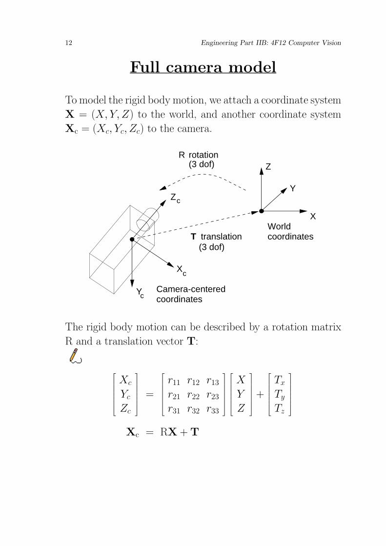
Full camera model

To model the rigid body motion, we attach a coordinate system

X = (X, Y, Z) to the world, and another coordinate system

Xc = (Xc, Yc, Zc) to the camera.


WorldcoordinatesT translation

(3 dof)

X

Y

Z

X

Z

Y

c

c

c

rotation(3 dof)

R

The rigid body motion can be described by a rotation matrix

R and a translation vector T:

Xc

Yc

Zc

=

r11 r12 r13r21 r22 r23r31 r32 r33

X

Y

Z

+

Tx

Ty

Tz

Xc = RX +T

Projection 13

Full camera model

As introduced before, planar perspective projection onto the

imaging surface is modelled by:

x =fXc

Zc

y =fYc

Zc


Worldcoordinates

Opticalaxis

Imageplane

Xc

Opticalcentre

Zc

X

Y

c

c

X

Y

Z

X

p

x

f


Full camera model

To model CCD imaging, we define pixel coordinatesw = (u, v)

in addition to the image plane coordinates x = (x, y).

(u , v )0 0

Optical axis

(0,511)

(0,0) (511,0)

(511,511)

CCD array

v

u

y

x

Image plane

w and x are related as follows:

u = u0 + kux , v = v0 + kvy

The overall mapping from world coordinates X to pixel coor-

dinates w = (u, v) is

u = u0 +kufXc

Zc= u0 +

kuf(r11X+r12Y +r13Z+Tx)

r31X+r32Y +r33Z+Tz

v = v0 +kvfYc

Zc= v0 +

kvf(r21X+r22Y +r23Z+Ty)

r31X+r32Y +r33Z+Tz

Projection 15

Homogeneous coordinates

The expressions at the foot of page 14 are messy! Homo-

geneous coordinates offer a more natural framework for

the study of projective geometry. The imaging process can be

expressed as a linear matrix operation in homogeneous coor-

dinates. Furthermore, a series of projections can be expressed

as a single matrix operation.

We usually express the location of a point in Cartesian coor-

dinates. In 2D space, for example, we would use coordinates

x = (x, y). Cartesian coordinates become cumbersome when

dealing with points at infinity, a crucial ingredient in the pro-

jection process. The Cartesian coordinates of a point at infin-

ity are in general both infinite but have a definite ratio x/y,

depending on the direction of the point from the origin. Cal-

culation with infinite quantities of this kind is confusing, and

it is convenient to represent each point not by two numbers

x = (x, y) but by three numbers x = (x1, x2, x3) such that

x

y

=

x1/x3x2/x3



If λ is any non-zero number, then (λx1, λx2, λx3) denotes the

same point as (x1, x2, x3): it is only the ratios of the ele-

ments of x that matter. If now x3 = 0, then x = x1/x3 and

y = x2/x3 are infinite but have the definite ratio x/y = x1/x2;

the numbers (x1, x2, 0) denote points at infinity, obviating cal-

culation with infinite coordinates.

Such a method of representing a point is called a homogeneous

coordinate system, because any equation in (x, y) is equivalent

to a homogeneous equation (ie. one in which all the terms are

of the same degree) in (x1, x2, x3). For instance, any line has

an equation of the form

a1x + a2y + a3 = 0

On substituting x1/x3 and x2/x3 for x and y, this becomes

a1x1x3

+ a2x2x3

+ a3 = 0

⇔ a1x1 + a2x2 + a3x3 = 0

The line at infinity, incidentally, also has an equation of this

form, namely x3 = 0.

Projection 17


Here are some further examples of homogeneous representa-

tions, this time using points in 3D space. To convert from

homogeneous to Cartesian coordinates, we take ratios:

(x1, x2, x3, x4) →

x1x4

,x2x4

,x3x4

X X

If x4 is zero, then X represents a point at infinity. X = 0 has

no meaning and is undefined.

To convert from Cartesian to homogeneous coordinates, we

add an extra dimension and introduce an arbitrary scaling:

(X, Y, Z) → (λX, λY, λZ, λ)

X X

By convention, λ is set to 1 (where possible).

To appreciate the power of homogeneous coordinates, we need

to study some examples, starting with the perspective projec-

tion of the point Xc = (Xc, Yc, Zc) onto the image plane x =

(x, y). In homogeneous coordinates we have Xc = (λXc, λYc, λZc, λ)

and x = (sx, sy, s).


Perspective projection revisited

Perspective projection can be expressed as

sx

sy

s

=

f 0 0 0

0 f 0 0

0 0 1 0

λXc

λYc

λZc

λ

or, equivalently,

x = Pp Xc , where Pp =

f 0 0 0

0 f 0 0

0 0 1 0

x is the homogeneous representation of the image point x.

Notice how perspective projection is a simple matrix multipli-

cation by Pp in homogeneous coordinates.

To check that the homogeneous representation of perspective

projection works, we can convert x into its Cartesian equivalent

x:

x =

x

y

=

sx/s

sy/s

=

fXc/Zc

fYc/Zc

Notice how the value of λ has no effect on the projection (we

would conventionally set λ to 1). Equivalently, the same pro-

jection is achieved by multiplying by µPp (µ 6= 0).

Projection 19

Exercise — horizon lines

As an exercise in the use of homogeneous coordinates, let’s

consider the two parallel planes

nxXc + nyYc + nzZc = d1

nxXc + nyYc + nzZc = d2 , d2 6= d1

and find the equation of their horizon line in the image. Con-

verting to homogeneous coordinates, points Xc = (Xc, Yc, Zc)

become Xc = (X1, X2, X3, X4), where

Xc

Yc

Zc

=

X1/X4

X2/X4

X3/X4

The homogeneous equations of the planes are

nxX1

X4+ ny

X2

X4+ nz

X3

X4= d1

⇔ nxX1 + nyX2 + nzX3 = d1X4

and nxX1 + nyX2 + nzX3 = d2X4

Notice that the planes intersect along a line at infinity, which

has a well-defined equation in homogeneous coordinates:

nxX1 + nyX2 + nzX3 = X4 = 0 (1)


Exercise — horizon lines

The image of a point Xc is given by

x =

x1x2x3

= Pp Xc =

fX1

fX2

X3

(2)

Combining (1) and (2) we obtain

nxx1f

+nyx2f

+ nzx3 = 0

⇔ nxx1 + nyx2 + fnzx3 = 0 (3)

This is the homogeneous equation of the horizon line in the

image.

To convert back to Cartesian image coordinates, we take ratios:

x =

x

y

=

x1/x3x2/x3

(4)

Combining (3) and (4) we obtain

nx x x3 + ny y x3 + f nz x3 = 0

⇔ nxx + nyy + fnz = 0

This is the Cartesian equation of the horizon line in the image.

The horizon of the ground plane can be found by setting nx =

0, ny = 1, nz = 0, which gives y = 0, as expected.

Projection 21

Camera projection matrix

Let’s look again at the full camera model, this time in homo-

geneous coordinates. We can construct a camera projection

matrix in three stages.

1. Rigid body transformation

There is a rigid body transformation between the world co-

ordinates X and the camera-centered coordinates Xc. This

accounts for rigid body motion between the camera and the

scene:

Xc

Yc

Zc

1

=

r11 r12 r13 Tx

r21 r22 r23 Ty

r31 r32 r33 Tz

0 0 0 1

X

Y

Z

1

or, equivalently,

Xc = Pr X , where Pr =

R T

0 0 0 1

X is the homogeneous representation of the world point X,

and likewise for Xc. Pr is the rigid body transformation matrix

(rotation and translation).



2. Perspective projection

The next stage is perspective projection of Xc onto x in the

image plane. We have already seen this on page 18:

sx

sy

s

=

f 0 0 0

0 f 0 0

0 0 1 0

Xc

Yc

Zc

1

or, equivalently,


f 0 0 0

0 f 0 0

0 0 1 0

x = (sx, sy, s) is the homogeneous representation of the image

point x = (x, y). Pp is the perspective projection matrix.

3. CCD imaging

Finally, we have to convert to pixel coordinates w = (u, v):

su

sv

s

=

ku 0 u00 kv v00 0 1

sx

sy

s

Projection 23


Equivalently,

w = Pc x , where Pc =

ku 0 u00 kv v00 0 1

w = (su, sv, s) is the homogeneous representation of the pixel

coordinates w = (u, v). Pc is the CCD calibration matrix.

We can now express the overall imaging process, from X to w,

as a single matrix multiplication in homogeneous coordinates:

w = PpsX

where Pps = PcPpPr

=

ku 0 u00 kv v00 0 1

f 0 0 0

0 f 0 0

0 0 1 0

R T

0 0 0 1

Pps is the camera projection matrix for a perspective camera.

It is a 3 × 4 matrix with 10 degrees of freedom1. The prod-

uct PcPp accounts for all the intrinsic (or internal) camera

parameters. Pr accounts for the extrinsic parameters.

1At first sight, it appears to have 11 degrees of freedom: 3 for R, 3 for T, and oneeach for f , ku, kv, u0 and v0. However, these parameters are not all independentin their effect on the projection. If you refer back to the equations at the foot ofpage 14, you should be able to see that f , ku, kv provide only 2 degrees of freedombetween them.


The projection matrix

The projection matrix, Pps is not a general 3×4 matrix, but

has a special structure composed of Pr, Pp and Pc. It can be

conveniently decomposed into the following two matrices – a

3×3 upper triangular matrix called the camera calibration

matrix K and a matrix representing the rigid-body motion:

Pps = K[R|T]

=

αu 0 u00 αv v00 0 1

r11 r12 r13 Tx

r21 r22 r23 Ty

r31 r32 r33 Tz

where the image scaling factors are αu = fku and αv = fkv.

The ratio αv/αu is known as the aspect ratio.

Projection 25

The projective camera

We could also consider another camera model, the projective

camera, which is described by the general 3× 4 matrix P:

w = PX, where P =

p11 p12 p13 p14p21 p22 p23 p24p31 p32 p33 p34

The projective camera has 11 degrees of freedom (since the

overall scale of P does not matter). It is often far more conve-

nient to deal with a projective camera than a perspective one,

since we do not have to worry about any nonlinear constraints

on the elements of P.

Since the perspective camera is a special case of the projective

camera, any results we derive for the projective camera will

also hold for the perspective camera.


Viewing a plane

Camera models can be simplified under restrictive viewing con-

ditions. Suppose, for example, we are viewing a planar scene

(a tabletop, for instance). The geometry of the scenario is

illustrated below.

World planeZ = 0

X

Y

Z

X

Z

Y

c

c

c

T translation

rotation(3 dof)

R

(3 dof)

Without loss of generality, assume that the plane we are view-

ing has equation Z = 0. The rigid body displacement between

the camera and the plane can be expressed in homogeneous

coordinates as

Xc

Yc

Zc

1

=

r11 r12 r13 Tx

r21 r22 r23 Ty

r31 r32 r33 Tz

0 0 0 1

X

Y

Z

1

Projection 27

Viewing a plane

However, we know that Z = 0, so we can reduce this to

Xc

Yc

Zc

1

=

r11 r12 Tx

r21 r22 Ty

r31 r32 Tz

0 0 1

X

Y

1

or, equivalently,

Xc = Ppr X

p , where Ppr =

r11 r12 Tx

r21 r22 Ty

r31 r32 Tz

0 0 1

Xp is the homogeneous representation of a point Xp = (X, Y )

on the world plane. Ppr is the planar rigid body transformation

matrix (rotation and translation).

The rest of the imaging process can be achieved using the same

perspective projection (Pp) and CCD imaging (Pc) matrices as

before.


Viewing a plane

The overall imaging process is:

w = PppsX

p

where Ppps = PcPpP

pr

=

ku 0 u00 kv v00 0 1

f 0 0 0

0 f 0 0

0 0 1 0

r11 r12 Tx

r21 r22 Ty

r31 r32 Tz

0 0 1

Ppps is the camera projection matrix for a perspective camera

viewing a plane. It is a 3 × 3 matrix with a special structure

composed of Ppr, Pp and Pc.

As with the 3D case, we can relax the constraints on the el-

ements of Ppps to obtain a more tractable camera model de-

scribed by the general 3× 3 matrix:

w = PpXp, where Pp =

p11 p12 p13p21 p22 p23p31 p32 p33

The transformation between w and Xp is known as a pla-

nar projective transformation or a homography or

collineation. It has 8 degrees of freedom (the scale of Pp does

not matter).

Projection 29

Viewing a line

Finally, we can consider the special case of viewing a world line.

Without loss of generality, assume we are interested in the line

defined by the world X-axis. The overall imaging process is:

w = PlpsX

l

where Plps =

ku 0 u00 kv v00 0 1

f 0 0 0

0 f 0 0

0 0 1 0

r11 Tx

r21 Ty

r31 Tz

0 1

Plps is the camera projection matrix for a perspective camera

viewing a line. It is a 3 × 2 matrix with a special structure

composed of Plr, Pp and Pc.

As with the 3D and 2D cases, we can relax the constraints on

the elements of Plps to obtain a more tractable camera model

described by the general 3× 2 matrix:

w = PlXl, where Pl =

p11 p12p21 p22p31 p32

This projective camera model has 5 degrees of freedom (since

the overall scale of Pl does not matter).


Planar transformations

1

4L

L

L23

3

L

L

l

l

l1

5

2

l45

l

C

Euclidean

c

1

4L

L

L23

5

l

L

l

Ll5

3

4

l21

lC

Similarity

c

1

4L

L

L23

5

L

3

lL

l2

l

4

l1

5

l

C

Affine c

1

4L

L

L23

5

L

1

L 2l3

l4

l5

l lC

Projective

c

Projection 31

Planar transformations

Planar transformations, geometry and invariants 2

Group Matrix Distortion Invariants

projective8 DOF

p11 p12 p13p21 p22 p23p31 p32 p33

concurrency andcollinearity, order ofcontact, tangentdiscontinuities and cusps,cross-ratio of four collinearpoints, measurements incanonical view

affine6 DOF

p11 p12 p13p21 p22 p230 0 p33

all the above, plusparallelism, ratio of areas,ratio of lengths on collinearor parallel lines(eg. midpoints)

similarity4 DOF

r11 r12 Tx

r21 r22 Ty

0 0 s

all the above, plus ratio oflengths, angle

Euclidean3 DOF

r11 r12 Tx

r21 r22 Ty

0 0 1

all the above, plus length,area

2Note that it is easy to show that a circle is transformed to an ellipse by the projective transformation,

H. In general a conic section is a quadratic in planar co-coordinates, au2+buv+cv2+du+ev+f = 0. It can

be expressed in homogeneous co-ordinates with a 3× 3 symmetric matrix: wTCw = 0. It is transformed

by the projective transformation into another conic section with matrix: C′ = H−TCH−1.


Camera calibration: 3D → 2D

Camera calibration is the name given to the process of

discovering the projection matrix (and its decomposition into

camera matrix and the position and orientation of the camera)

from an image of a controlled scene. For example, we might

set up the camera to view a calibrated grid of some sort.

Projection 33

Camera Calibration

X

Y

Z

X

Z

Y

c

c

c

P?

Controlled 3D scene

For a projective camera we have:

su

sv

s

=

p11 p12 p13 p14p21 p22 p23 p24p31 p32 p33 p34

X

Y

Z

1

There are 11 parameters to estimate (since the overall scale of

P does not matter, we could, for example, either set p34 to 1

or |p| = 1).


Camera Calibration

Each point we observe gives us a pair of equations:

ui =suis

=p11Xi + p12Yi + p13Zi + p14p31Xi + p32Yi + p33Zi + p34

vi =svis

=p21Xi + p22Yi + p23Zi + p24p31Xi + p32Yi + p33Zi + p34

Since we are observing a calibrated scene, we know Xi, Yi, and

Zi, and we observe the pixel coordinates ui and vi in the im-

age. The equations above can be rearranged to give two linear

equations in the unknown projection matrix parameters.3

Since there are 11 unknowns, we need to observe at least 6

points to calibrate the camera. The equations can be solved

using linear least squares. Note how the use of the projective

camera has linearized the problem.

3For n calibration points and their corresponding image projections we have 2n equations in the form

Ap = 0:

X1 Y1 Z1 1 0 0 0 0 −u1X1 −u1Y1 −u1Z1 −u1

0 0 0 0 X1 Y1 Z1 1 −v1X1 −v1Y1 −v1Z1 −v1...

......

......

......

......

......

...

Xn Yn Zn 1 0 0 0 0 −unXn −unYn −unZn −un

0 0 0 0 Xn Yn Zn 1 −vnXn −vnYn −vnZn −vn

p11p12p13p14p21p22p23p24p31p32p33p34

= 0

Projection 35

Camera Calibration

The linear solution is, however, only approximate and should

ideally be used as the starting point for non-linear minimisa-

tion: i.e. finding the parameters of the projection matrix that

minimise the errors between measured image points, (ui, vi)

and projected (or modelled) image positions, ((ui, vi):

minP

∑

i((ui − ui)

2 + (vi − vi)2)

Having obtained the projection matrix it is possible to decom-

pose it into the camera calibration matrix and the orientation

and position of the camera (if necessary):

Pps = K[R|T]

Standard matrix techniques exist for decomposing the 3× 3

sub-matrix into the product of an upper triangular matrix, K,

and a rotation (orthogonal) matrix R (known as QR decom-

positon).

The translation vector or position of the camera can then be

obtained by:

T = K−1(p14, p24, p34)T



To calibrate the camera for viewing planar scenes, we could

set up the camera to view some sort of calibrated planar grid.

X

Y

X

Z

Y

c

c

c

Controlled 2D scene

P ?p

For a plane to plane projectivity, we have

su

sv

s

=

p11 p12 p13p21 p22 p23p31 p32 p33

X

Y

1

There are 8 parameters to estimate (if we set, for example,

either |p| = 1 or p33 to 1), and each observed point gives us a

pair of linear equations, so we need to observe at least 4 points.

Again, we use linear least squares to solve for the elements of

Pp.

Projection 37


Finally, we consider the calibration of a camera viewing a line.

This is accomplished by viewing a line with some markings at

known positions.

X

Z

Y

c

c

c

P ?

X

Controlled 1D scene

l

For a projective camera we have

su

sv

s

=

p11 p12p21 p22p31 p32

X

1

There are 5 parameters to estimate (if we set, for example,

p32 to 1), and each observed point gives us a pair of linear

equations, so we need to observe at least 3 points. Again, we

use linear least squares to solve for the elements of Pl.


Recovery of world position

With a calibrated camera, we can attempt to recover the world

position of image features.

1D case (line to line): given u, we can uniquely determine

the position of the point on the line.

su

s

=

p11 p12p31 p32

X

1

⇔ u =su

s=

p11X + p12p31X + p32

⇔ X =p32u− p12−p31u + p11

2D case (plane to plane): given u and v, we can uniquely

determine the position of the point on the world plane. For a

plane to plane projectivity, we have

u

v

1

=

p11 p12 p13p21 p22 p23p31 p32 p33

λX

λY

λ

⇔

λX

λY

λ

=

p11 p12 p13p21 p22 p23p31 p32 p33

−1

u

v

1

⇔ X =pi11u + pi12v + pi13pi31u + pi32v + pi33

, Y =pi21u + pi22v + pi23pi31u + pi32v + pi33

Projection 39

Recovery of world position

3D case (3D world to image plane): given u and v,

we cannot uniquely determine the position of the point in the

world.

su

sv

s

=

p11 p12 p13 p14p21 p22 p23 p24p31 p32 p33 p34

X

Y

Z

1

⇒ u =su

s=

p11X + p12Y + p13Z + p14p31X + p32Y + p33Z + p34

⇒ v =sv

s=

p21X + p22Y + p23Z + p24p31X + p32Y + p33Z + p34

Each observed image point (u, v) gives us two equations in

three unknowns (X, Y, Z). These equations define a line (ie. a

ray) in space, on which the world point must lie.

For general 3D scene interpretation, we need to use more than

one view. Later in the course we will take a detailed look at

stereo vision and structure from motion.


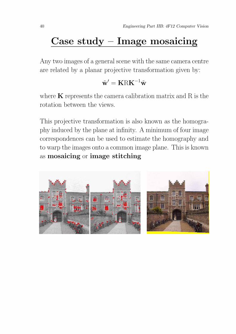
Case study – Image mosaicing

Any two images of a general scene with the same camera centre

are related by a planar projective transformation given by:

w′ = KRK−1w

whereK represents the camera calibration matrix and R is the

rotation between the views.

This projective transformation is also known as the homogra-

phy induced by the plane at infinity. A minimum of four image

correspondences can be used to estimate the homography and

to warp the images onto a common image plane. This is known

as mosaicing or image stitching

Projection 41

Matching with outlier data - RANSAC

The RANSAC algorithm (Fischler and Bolles (1981)) is an

algorithm for robust fitting of models in the presence of many

data outliers. The algorithm is very simple.


Case study – Photobuilder

Vanishing points corresponding to three orthogonal directions

can be used to recover the projection matrix of the viewpoint

(Cipolla et al (1999)).

3. Finding vanishing points and camera calibration

1. Original uncalibrated photographs

4. Computation of projection matrices and camera motion

2. Primitive definition and localisation

R + T

5. Triangulation, 3D reconstruction and texture mapping

Projection 43

Parallel projection

Recall that we have seen plenty of CCD images which appear

to have been formed by orthographic projection. For example:

Orthographic? Certainly not orthographic

It might be useful to analyse what is special about the image on

the left. This will allow us to identify a simpler, more tractable

camera model for use under certain viewing conditions.

It appears that parallel projection is a good approximation

when the depth of the objects in the scene is small compared

with the distance of the camera from the scene. On the left all

the objects are within a narrow depth band, so ∆Zc is small

compared to Zc. On the right there is a large depth variation

∆Zc in the image.


Parallel projection

Recall that perspective projection is

sx

sy

s

=

f 0 0 0

0 f 0 0

0 0 1 0

Xc

Yc

Zc

1

or, equivalently,


f 0 0 0

0 f 0 0

0 0 1 0

The only component of x that depends on Zc is the scaling

term, s. If we consider Zc as approximately constant for all

objects in the scene, so that Zc = Zavc , we can rewrite the

projection as

sx

sy

s

=

f 0 0 0

0 f 0 0

0 0 0 Zavc

Xc

Yc

Zc

1

or, equivalently,

x = Ppll Xc , where Ppll =

f 0 0 0

0 f 0 0

0 0 0 Zavc

This is called weak perspective projection.

Projection 45

Weak perspective

We can now derive the form of the overall weak perspective

projection matrix from world coordinates X to pixel coordi-

nates w.

Following an identical derivation to the one we used in the per-

spective case on page 23, but inserting the parallel projection

matrix Ppll in place of the perspective matrix Pp, we obtain

w = PwpX

where Pwp = PcPpllPr

=

ku 0 u00 kv v00 0 1

f 0 0 0

0 f 0 0

0 0 0 Zavc

R T

0 0 0 1

=

fkur11 fkur12 fkur13 fkuTx + u0Zavc

fkvr21 fkvr22 fkvr23 fkvTy + v0Zavc

0 0 0 Zavc

Pwp is the projection matrix for a weak perspective camera. It

is a 3× 4 matrix with a special structure composed of Pr, Ppll

and Pc.


The affine camera

As usual, we prefer to discard the nonlinear constraints on the

elements and consider the general 3× 4 matrix of this form:

Paff =

p11 p12 p13 p14p21 p22 p23 p240 0 0 p34

Paff is the projection matrix for the affine camera. It has

8 degrees of freedom (since the overall scale of Paff does not

matter). If we set p34 to 1, we can write the projection as

su

sv

s

=

p11 p12 p13 p14p21 p22 p23 p240 0 0 1

X

Y

Z

1

⇒

u

v

=

p11 p12 p13 p14p21 p22 p23 p24

X

Y

Z

1

We therefore need only 4 points to calibrate an affine camera

(compare with 6 points for the full projective camera). This is

one of the principle attractions of using an affine camera where

appropriate. Note that the affine camera is linear.

Projection 47

Planar weak perspective

We can also consider a weak perspective camera viewing a

plane. This would be a good model to use when the plane in

the image has little depth variation compared with the viewing

distance.

Following an identical derivation to the one we used in the per-

spective case on page 28, but inserting the parallel projection

matrix Ppll in place of the perspective matrix Pp, we obtain

w = PpwpX

p

where Ppwp = PcPpllP

pr

=

ku 0 u00 kv v00 0 1

f 0 0 0

0 f 0 0

0 0 0 Zavc

r11 r12 Tx

r21 r22 Ty

r31 r32 Tz

0 0 1

=

fkur11 fkur12 fkuTx + u0Zacc

fkvr21 fkvr22 fkvTy + v0Zacc

0 0 Zavc

Ppwp is the projection matrix for a weak perspective camera

viewing a plane. It is a 3 × 4 matrix with a special structure

composed of Ppr, Ppll and Pc.


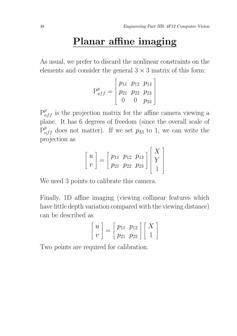
Planar affine imaging

As usual, we prefer to discard the nonlinear constraints on the

elements and consider the general 3× 3 matrix of this form:

Ppaff =

p11 p12 p13p21 p22 p230 0 p33

Ppaff is the projection matrix for the affine camera viewing a

plane. It has 6 degrees of freedom (since the overall scale of

Ppaff does not matter). If we set p33 to 1, we can write the

projection as

u

v

=

p11 p12 p13p21 p22 p23

X

Y

1

We need 3 points to calibrate this camera.

Finally, 1D affine imaging (viewing collinear features which

have little depth variation compared with the viewing distance)

can be described as

u

v

=

p11 p12p21 p22

X

1

Two points are required for calibration.

Projection 49

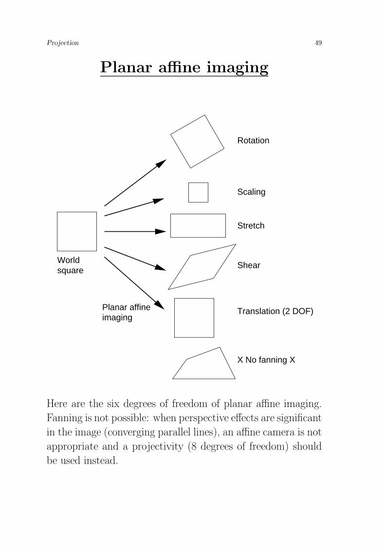
Planar affine imaging

Worldsquare

Planar affineimaging

Rotation

Scaling

Stretch

Translation (2 DOF)

Shear

X No fanning X

Here are the six degrees of freedom of planar affine imaging.

Fanning is not possible: when perspective effects are significant

in the image (converging parallel lines), an affine camera is not

appropriate and a projectivity (8 degrees of freedom) should

be used instead.


Geometric Invariants - cross-ratio

To find a numerical invariant, we start with the simplest pro-

jective case, that of viewing a line. Recall that the image

u-coordinate of a point X on the line is given by

su

s

=

p11 p12p31 1

X

1

la

lb

lc ld

u

v

Image d

c

a

b

o

The figure shows the image of four world points A, B, C and

D, and the world origin O. Distances l measured along the

image line from o are linear functions of u and can therefore

be expressed as

sl

s

=

p q

r 1

X

1

Projection 51

The cross-ratio

Hence we obtain

li =pXi + q

rXi + 1

Let’s investigate whether the ratios of lengths along the line

are invariant.

lc − la =(Xc −Xa)(p− qr)

(rXc + 1)(rXa + 1)

lc − lb =(Xc −Xb)(p− qr)

(rXc + 1)(rXb + 1)

⇒lc − lalc − lb

=(Xc −Xa)(rXb + 1)

(Xc −Xb)(rXa + 1)(5)

So the ratios of lengths are not invariant (compare with the

affine case, where they are).

Similarly,ld − lald − lb

=(Xd −Xa)(rXb + 1)

(Xd −Xb)(rXa + 1)(6)

Dividing (6) by (5) we obtain

(ld − la)(lc − lb)

(ld − lb)(lc − la)=

(Xd −Xa)(Xc −Xb)

(Xd −Xb)(Xc −Xa)

This is the cross-ratio, which is invariant.


The cross-ratio: example

Let’s check the cross-ratio by constructing a line to line per-

spective projection and measuring lengths.

Oc

ab

c d

A

C

D

B

Lengths measured with a ruler are:

AD = 77.5mm, BC = 15.0mm, BD = 38.5mm, AC = 54.0mm

ad = 48.5mm, bc = 7.0mm, bd = 14.5mm, ac = 41.0mm

Forming the cross-ratios gives:

AD ×BC

BD ×AC= 0.56 ,

ad× bc

bd× ac= 0.57

So the cross-ratios agree to within experimental accuracy.

Projection 53

Five point invariants on the plane

Even though we have developed the cross-ratio for four points

on a line, we can also use it in planar imaging situations. We

need 5 distinguished points to form invariants on the plane.

e1

a

c

d

e

g

f

Cleverconstructions

a

c

d

e

2b b

e

Given the image of the 5 points a . . . e, we can use the invariant

property of intersection to find 4 more distinguished points:

f, the intersection of the extrapolated lines a-b and d-c; g,

similarly; e1, the intersection of the line joining f and e with

the side a-d, and e2 similarly. We can now form two cross-

ratios:

δ1 = cross-ratio of {a, e2, b, f}

δ2 = cross-ratio of {a, e1, d, g}

These will be the same measured in any view of the 5 points.


Five point invariants on the plane

Here’s an example of how we could use the five point invariants

for object recognition.

1l l2

l l

l

45

c3

2

1e

l

e

l2 l3 l4

l51 c

e2

1e

cr (a , b , e , f)2

e

b

d

g

a

a

f

gec

d

f

c

b

cr (a , e , d , g)1

We identify five distinguished points a . . . e at the corners of

the bracket and construct intersections to find four more dis-

tinguished points f, g, e1 and e2. We now have two sets of four

collinear points, {a, b, e2, f} and {a, e1, d, g}, for which we can

calculate cross-ratios. These will be the same in any view, and

can be used to identify the bracket. Other configurations of

five planar points will yield different cross-ratios.

Projection 55

Further Reading - Canonical Views

Another way to form projective invariants for 5 coplanar points

uses a calibration-like procedure. For a plane to plane projec-

tivity, we have

w = PpXp

where Pp is a 3 × 3 matrix. It follows that any two views of

the plane are related by a projectivity. If w′ is another view,

then

w′ = Pp′Xp = Pp′[Pp]−1w = Pp′′w

So the two views w and w′ are related by a projectivity Pp′′.

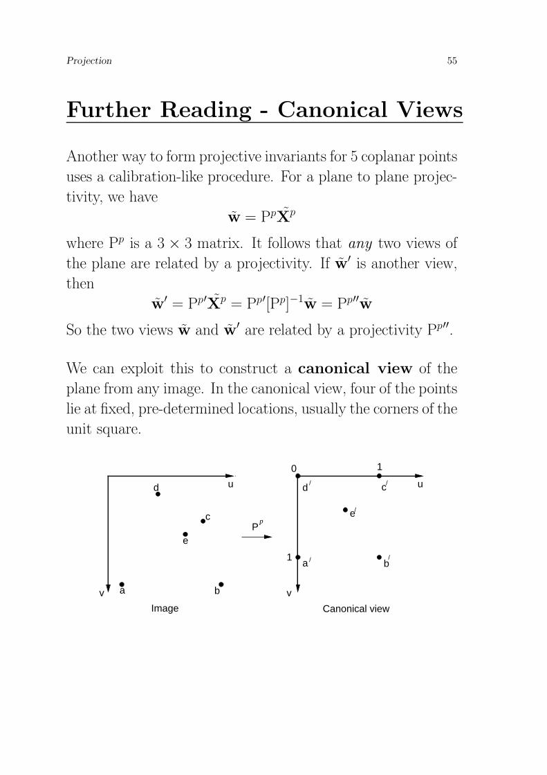
We can exploit this to construct a canonical view of the

plane from any image. In the canonical view, four of the points

lie at fixed, pre-determined locations, usually the corners of the

unit square.

v

u

pP

c/d

/

e/

b/

a /

a

c

d

e

b

u

10

1

v

Image Canonical view


Canonical views

a . . . d are the four distinguished points, and we use their co-

ordinates in the image to find the 3× 3 projectivity Pp which

maps them onto the corners of the unit square in the canonical

view. This is simply a calibration process. If we then apply the

projectivity Pp to the 5th point e, its coordinates u and v in

the canonical view provide us with two projective invariants.

Canonical views have proved very successful for recognition of

planar objects. Four distinguished points are used to map the

structure in the image into a canonical view. In the canonical

view, the structure is compared with a model library to spot

any match.

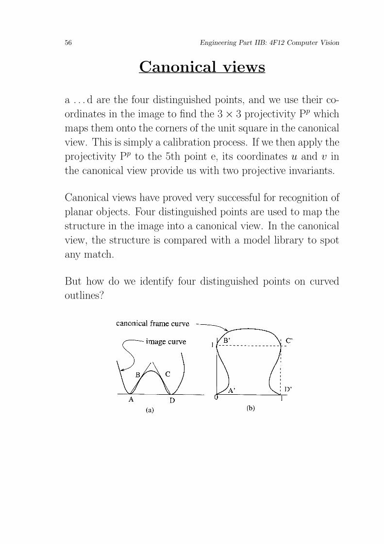
But how do we identify four distinguished points on curved

outlines?

Projection 57

Canonical views

There is a nice construction which works for curve segments

with concavities (many industrial parts). The bitangent across

the concavity gives us two distinguished points A and D, then

the tangents cast from A and D into the concavity give us

another two, B and C.

Next we find the projectivity Pp which maps A, B, C and D

onto the corners of the unit square in the canonical view, and

the rest of the curve is mapped into the canonical view using

Pp. What we end up with is an invariant signature of the

curve in the canonical view.


Canonical views

As expected, the construction produces the same signature for

3 different views of the spanner . . .

. . . and different signatures for different objects.

Projection 59

Summary

3D → 2D camera models

Perspective

w = PcPpPrX = PpsX. Tricky to calibrate.

susvs

=

ku 0 u0

0 kv v00 0 1

f 0 0 00 f 0 00 0 1 0

r11 r12 r13 Tx

r21 r22 r23 Ty

r31 r32 r33 Tz

0 0 0 1

XYZ1

Projective

w = PX. 11 degrees of freedom (p34 = 1). 6 points to calibrate.

susvs

=

p11 p12 p13 p14p21 p22 p23 p24p31 p32 p33 p34

XYZ1

Weak perspective

w = PcPpllPrX = PwpX. Tricky to calibrate.

susvs

=

ku 0 u0

0 kv v00 0 1

f 0 0 00 f 0 00 0 0 Zav

c

r11 r12 r13 Tx

r21 r22 r23 Ty

r31 r32 r33 Tz

0 0 0 1

XYZ1

Affine

w = Paff X. 8 degrees of freedom (p34 = 1). 4 points to calibrate.

susvs

=

p11 p12 p13 p14p21 p22 p23 p240 0 0 p34

XYZ1


Summary


Perspective

w = PcPpPprX

p = PppsX

p. Tricky to calibrate.

susvs

=

ku 0 u0

0 kv v00 0 1

f 0 0 00 f 0 00 0 1 0

r11 r12 Tx

r21 r22 Ty

r31 r32 Tz

0 0 1

XY1

Projective

w = PpXp. 8 degrees of freedom (p33 = 1). 4 points to calibrate.

susvs

=

p11 p12 p13p21 p22 p23p31 p32 p33

XY1

Weak perspective

w = PcPpllPprXp = Pp

wpXp. Tricky to calibrate.

susvs

=

ku 0 u0

0 kv v00 0 1

f 0 0 00 f 0 00 0 0 Zav

c

r11 r12 Tx

r21 r22 Ty

r31 r32 Tz

0 0 1

XY1

Affine

w = Ppaff X

p. 6 degrees of freedom (p33 = 1). 3 points to calibrate.

susvs

=

p11 p12 p13p21 p22 p230 0 p33

XY1

Projection 61

Summary


Perspective

w = PcPpPlrX

l = PlpsX

l. Tricky to calibrate.

susvs

=

ku 0 u0

0 kv v00 0 1

f 0 0 00 f 0 00 0 1 0

r11 Tx

r21 Ty

r31 Tz

0 1

[

X1

]

Projective

w = PlXl. 5 degrees of freedom (p32 = 1). 3 points to calibrate.

susvs

=

p11 p12p21 p22p31 p32

[

X1

]

Weak perspective

w = PcPpllPlrX

l = PlwpX

l. Tricky to calibrate.

susvs

=

ku 0 u0

0 kv v00 0 1

f 0 0 00 f 0 00 0 0 Zav

c

r11 Tx

r21 Ty

r31 Tz

0 1

[

X1

]

Affine

w = Plaff X

l. 4 degrees of freedom (p32 = 1). 2 points to calibrate.

susvs

=

p11 p12p21 p220 p32

[

X1

]


BibliographySome of the figures were taken from the following, which make goodfurther reading.

History of perspective

M. Kemp. The Science of Art. Yale University Press, 1990.

Projective geometry

J. L. Mundy and A. Zisserman. Projective geometry for machinevision. In J. L. Mundy and A. Zisserman, eds. Geometrical Invariance

in Computer Vision. MIT Press, 1992. (Figures on page 8.)

Invariants

J. L. Mundy and A. Zisserman, eds. Geometrical Invariance in Com-

puter Vision. MIT Press, 1992. (Figures on pages 30, 54, 56, 57, 58.)

Camera calibration and projection matricesR. Cipolla and P. Giblin Visual Motion of Curves and Surfaces. CUP,

1999.

university of cambridge engineering part iib module 4f12

Documents