university of nigeria buckling of imperfection... · assumed initial imperfections of various sizes...
TRANSCRIPT

University of Nigeria Research Publications
ETTE, Anthony Monday PG/Ph.D-82-1731
Aut
hor
Title
Dynamic Buckling Of Imperfection-Sensitive Elastic Structures Under Slowly-
Varying Time Dependent Loading
Facu
lty
Physical Science
Dep
artm
ent
Mathematics
Dat
e
1990

DYNAMIC BUCKLING OF nPERFECTION-SENSITIVE ELASTIC STRUCTURES
UNDER SLOWLY-VARYING TIME DEPENDENT LOADING
by
AhrnONY MONDAY E m
PG/Ph.D/82/173 1
SUBMITTED IN PARTIAL FULFlLMENT OF THE REQUIREMENT FOR THE
AWARD OF THE DECREE OF DOCTOR OF PHILOSOPHY IN MATHEMATICS OF
THE UNIVERSITY OF NIGERLA
SUPERVISOR: PROFESSOR J.C. AMAUGO, FAS

ANTHONY MONDAY ETTE, a Postgraduate student in the Department of Mathematics
and with Reg. No. PG/Ph.D/82/1731 has satisfactorily completed the requirements for
course and research work for the degree of DOCTOR OF PHILOSOPHY in
MATHEMATICS. The work embodied in this thesis is original and has not been
submitted in part or full for any other diploma or degree of this or any other University.
, I/ DR: G.C. CHUKWUMAH Head of Department
R J.C. AMAZIGO Supervisor

1 ACKVOWLEDGEMENT
I
I I wish to express my gratitude to my supervisor, Professor J.C. Amazigo for
methodically directing and guiding my sense of direction in the cause of the research
reported in this thesis. 1 wish in particular to express my heart-felt appreciation to him for
stimulating and motivating my interest in Applied Mathematics and for his deep-seated
understanding of the predicaments and constraint facing a typical Third World research
environment. He is to me, in every unqualified sense a complete gentleman, a friend, a
teacher and above all, a mathematician per excellence.
My unreserved indebtedness also goes to my friend Dr. Moses Oludotun Oyesanya, his
wife, Jumoke, and their children for their unqualified hospitality to me. Words cannot
adequately describe the numerous helps, motivational advice and scholarly encouragement
which this noble compatible pair and other members of their household rendered to me
especially in the darkest moment of greatest despair. They proved to me, in all honesty,
friends in need and friends indeed.

TABLE OF CONTENTS
TITLE PAGE
CERTIFICATION AND APPROVAL PAGE DEDICATION
ACKNOWLEDGEMENT
ABSTRACT
INTRODUCI'ION
CHAPTER
1 DYNAMIC BUCKLING OF A CUBIC MODEL
1 . 1 Formulation of the equation
1.2 Static Problem
1.3 Dynamic Problem - Step Loading
1.4 Slowly-varying Loading
2 DYNAMIC BUCLKING OF A CUBIC MODEL - SPECIAL CASES
2.1 Determination of the dynamic buckling load of the imperfect model structure for the case 6 = c.
2.2 Determination of the dynamic buckling load of the imperfect model structure for the case 6 = f 2 .
3 DETERMINATION OF THE DYNAMIC BUCKLING LOAD OF A
SPHERICAL CAP SUBJECTED TO A SLOWLY VARYING TIME
DEPENDENT LOADING
3.1 Derivation of the equation
3.2 Solution of the problem
4 DISCUSSION OF RESULTS
REFERENCES
FIGURES
TABLES

ABSTRACT
The dynamic buckling loads of some imperfection-sensitive elastic structures subjected
to slowly varying time dependent loading are determined using perturbation procedures.
First, we consider an elastically imperfect column resting on a softening nonlinear elastic
foundation. The governing differential equation has two small parameters. We determine
the dynamic buckling load of this column subjected to the stipulated loading for three
different cases. The cases are when the small parameters are not related and when they are
related first linearly and next quadratically in some way.
This idea is next applied to an elastically imperfect spherical cap and the dynamic
buckling load of the cap subjected to a slowly varying time dependent loading is
determined. The result shows, among other things, that for the case of the cap, the
coupling term has no significant contribution to the initial post-buckling phenomenon.
By assuming, in the results, that the slowly varying loading function is numerically
unity, we obtain the associated step loading results for both the column and the spherical
cap. These latter results confirm existing results for columns under step loading and
establish new ones for the spherical cap.

INTRODUCTION
The determination of the dynamic buckling load of an imperfection-sensitive elastic
structure under various time dependent loading histories has been an area of intense study
ever since Budiansky and Hutchinson, [2, 4, 61 extended the original work of Koiter on
static theory of post buckhg behaviour of elastic structures to the case of dynamic loading.
So far many of the studies in this area have concentrated primarily on the cases where the
time dependent loading is either step loading [2, 3,4, 7, 8, 11-17], impulsive loading [4,
61, or periodic loading [7]. Besides the periodic case, there has been a dearth of analytic
studies for the cases where the loading is essentially time dependent. The exceptions are
contained in [4,6] where rectangular and triangular loadings are considered.
Existing literature on the subject shows that dynamic buckling of imperfection-sensitive
elastic materials is usually modelled by nonlinear differential equations and that geometrical
imperfections in these materials are responsible for large scale reductions in their structural
strength. Our aim is to calculate the dynamic buckling loads of these structures from the
associated dynamic differential equations under certain prescribed initial and boundary
conditions and from these results, predict to what extent these geometrical imperfections
influence the buckling strength of the structures. Many of the earlier works on dynamic
buckling of elastic structures have sought to correlate reductions in buckling strength with
assumed initial imperfections of various sizes and shapes. The primary aim in such studies
has been that the results so obtained should provide qualitative information needed for a
statistical theory of buckling.
In many analytical studies [2, 4, 6 , 7, 81, it has become the practice to relate the
dynamic buckling stre.ngth of a given imperfect structure to its static strength so as to avoid

the repetitions of solving the problems on dynamic buckling for different imperfecrion-
sensitive structures under various imperfections for each different kind of loading.
Although the static buckling theory of an imperfection-sensitive structure is well
understood the accurate theory and proper understanding as well as the universal definition
of the mechanism of dynamic buckling are yet to be fully appreciated and formulated. As a
result, there is no consensus as to what constitutes "dynamic buckling".
As in other branches of Mechanics, analytical and numerical methods are the two basic
methods of solution of problems on dynamic buckling. Notable among solutions that have
used essentially analytical method are the works of Budiansky and Hutchinson [2, 4, 61,
Amazigo and Lockhart [l 1, 13, 141, Amazigo [12], Amazigo and Frank [3] and Danielson
[8]. It must however be pointed out that because of the non-linearity that has so far
characterized the resultant dynamic differential equations involved, the analytical
determination of the dynamic buckling load may present formidable difficulty. In some
cases [2,4], the analytical determination of the dynamic buckling load is preceded by first
simplifying the governing differential equations and discretizing the already continuous
system. The danger here as pointed out by Tamura and Babcock [16], is that the discrete
models tend to display static equilibrium positions which the continuous structure did not
possess. In some cases, analytical determination of the dynamic buckling load is first
accomplished by simplifying the modelling as done by Budiansky and Hutchinson [2 ,4]
and Danielson [8] while in some other cases this is done by enacting some simplifying
assumptions on the differential equations as done by Danielson [8]:
There have been several numerical solutions for some dynamic buckling problems.
Notable is the work of Svalbonas and Kalnins [7] who developed new computer
programmes for dynamic buckling loads of shells under general time dependent loading

and them compared and evaluated existing :~nalytical and numerical solurions for a specific
problem - the dynamic stability of spherical caps subjected to uniform step loading. They
showed that for certain classes of structures, the analytic solutions based on simple
dynamic buckling model approach of Budiansky and Hutchinson [2,4] and Danielson [8]
may be appropriately modified to give accurate buckling predictions. Other notable
numerical works in this regard include Tamura and Babcock [16], Fisher and Bert [17],
and Roth and Klosner [13].
In this work, we first consider a model problem consisting of a two-bar simply
supported column subjected to an axially applied step loading and next, the same model
under a slowly varying time dependent loading Af (6t) which varies only slightly over a
natural period of oscillation of the structure. Using phase plane analysis, we determine the
dynamic buckling load of the structure under the applied step loading in the first case. The
resulting differential equations in the second case contain two small parameters f and 6
where 5 << 1, 6 << 1 and A is the load parameters. Here
(0.01) f(0) = 1
(0.02) If(Gt)l s 1, r 2 O
By using a novel generalization of Lindstedt-Poincare method and initially assuming
that Gand 5 are not related, a two timing regular perturbation expansion in G and 5 gives a
uniformly valid solution of the dynamic response (displacement) of the system. We next
find the maximum displacement, reverse the series of maximum displacement in a manner
suggested in [ I , 12,201 and finally invoke the condition for dynamic buckling to determine
the dynamic buckling load of the model structure under slowly varying time dependent
loading.
We next assume that Gand 5 are related such that

(0.03) s = p = where a is real and constant. We determine the dynamic buckling loads for a = 1 and a =
2 and show in each case that the dynamic buckling load of the model structure under step
loading can be derived from these two cases by setting f (61) = 1 in the results for a = 1
and a = 2.
Lastly, we consider an imperfect spherical cap subjected to a time dependent slowly
varying loading ilf(6r). The imperfection is assumed to be both axisymmetric and
unsymmetric. By neglecting both the prebuckling inertia and the axisymmetric
imperfection and assuming homogeneous initial conditions, we determine analytically the
dynamic buckling load of the spherical cap under the stipulated loading. By setting
f (St) = 1 in the results obtained we specialize these results to the step loading case. We
compare these step loading results with the only existing analytical (approximate) results
obtained earlier by Budiansky and Hutchinson [2,4] and show that the results obtained in
the work reported here are conservative.

CHAPTER ONE
DYNAMIC BUCKLING OF A CUBIC MODEL
A simple model which is typical of this type of structure is a two-bar simply supported
column subjected to an axial load P(T) applied at T = 0. The bars are of length L, rigid and
weightless and carrying a mass M at the centre hinge whose motion is restrained by a
nonlinear softening spring that provides a restoring force KL(x - P x ~ ) , P > 0 where x is
the central hinges displacement. The initial displacement X plays the role of an
imperfection (See Fig. 1).
1.1 Formulation of the Equation
Let Q be the tension on each of the two arms of the column and 8 be a small angular
displacement of either bar from the neutral vertical position. We note that for small angular
displacement
For equilibrium of the point of application of the dynamic load in the axial direction, we get
For motion of the mass M, we have
(1.103) MX = 2 ~ s i n 8 - KL(X -px3), d'
('1 = -0. dT
Neglecting nonlinear geometric effects (cos 8 = 1, sin 8 -- 8) and eliminating Q between
(1.102) and (1.103) using (1.101) gives
We introduce the following non-dimensional quantities

where 5 << 1, 6 << 1.
The differential equation (1.104) and associated initial conditions become
(1.1OSa) ii + (1 - Af (6t))5 - b t 3 = Acf(6r),
(1.1OSb) ~ ( 0 ) = ((0) = 0
where b = f l ~ ~ > 0.
A is the load parameter. f (6t) is a slowly varying continuous function of t with right hand
derivatives of all orders at t = 0 and satisfying
(1.106) f(O)=l, If(6t)l<-l, r 20 .
The problem (1.105) is said to be that of a cubic model because of the cubic
nonlinearity. It models many important physical structures and the method of its solution
will be used to solve the problem on a spherical cap which essentially is a quadratic
structure.
We shall first find a solution for the static case corresponding to (1.105).
1.2 Static Problem
The static problem corresponding to (1.1 05) is
(1.201) (1 -1) t - b t 3 = A t where, in this case f (St) E 1 and 4' = 0.
Equation (1.201) is a nonlinear algebraic equation and for = 0 it becomes an eigenvalue
problem with solutions
(1.202a) 5 = 0
for all A and
(1.202b) ~ = l - b ( ~

3
a = 1 is called the classical buckling load for the perfect structure. For this case 5 = 0, the
curve of A versus 5 is symmetrical in 5 about the axis with zero slope at 5 = 0, while for
5 + 0 , the static buckling of the imperfect structure is independent of the sign of 5. By
setting a = 0 in (1.201) we get 4
where A, denotes the static buckling load of the imperfect structure.
1.3 Dynamic Problem - S t e ~ load in^
We now study the problem (1.105) where the loading is step loading. In this case f(&)
= 1 and the resulting differential equation is
(1.301a) j ' + ( l - ~ ) ( - b ( ~ = ~ 5 , r > O
(1.301 b) {(o) = ((0) = 0
The solution of (1.301) is important because step loading is a special case of a slowly
varying loading. Hence, an analytical solution of (1.301) will automatically shed some
light on the solution of (1.105).
A first integral of (1.301a) gives
The maximum value, 5, of 5 is obtained when 6 = 0. Thus, for 5, t 0, we obtain
There exists a maximum value of A for which a bounded value for the displacement 5, exists and it is this maximum value that is defined as the dynamic buckling load AD. This

dl, critical' value itD satisfies = 0 and f o r il greater than itD, the response is
d~ a
monotonic and unbounded. Thus from (1.304) or (1.303) we obtain
We shall now develop a perturbation scheme for the analytic solution of (1.301). We
proceed by first obtaining a uniformly valid perturbation solution of (1.301) in terms of the
load parameter A. The amplitude of the bounded solution is then obtained and A is next
maximized with respect to this amplitude. Following Lindstedt-Poincare method [I, 51, we
introduce a time scale i defined by
(1.306) i = (1 -1)"~(1+ w2c2 + U ~ F ~ + - - ) ~
Thus, we get
Substituting (1.306) and (1.307) into (1.301) we obtain
We shall now expand 6 in a Taylor series in the parameter namely
Substituting (1.309) into (1.308) and equating like powers of 5, we get

etc. The associated initial conditions are
Solving (1.3lOa), we obtain P,
Therefore, we get
(1.313) A
(i) = - cosl).
The solution of (1.310b) is
(1.314) 52 (f) s 0
We now substitute into (1.310~) and obtain
202a cosi + (1.315) L53 = -- 3 cost + -cos2t - -cos3l
1 -a 2 4 I To ensure a uniformly valid solution for t3 in l we equate to zero the coefficient of cosi in
(1.315) and so obtain
Thus, solving for t3(i) using (1.3lOd) gives
(1.317) 65ba3
53(') = - 32(1 - 2 )4 COST + ba3 [ 5 1 cos 2t + - cos 3i ( 1 4 2 2 32 1
So far, we see that to order c3, the displacement { ( t ) can be written as
(1.318) ((0 = t l(X + 5 2 ( X 2 + t 3 f 3

6
The amplitude, 5 , of the dynamic response is d5 the value of 5 ( t a ) such that -(i, ) = 0 . dt
This is given by
(1.319) 2Ac 4 b A 3 6 + ( 1 - 1 1 4 , valid for i = r .
The dynamic buckling load of the cubic model under step loading is thus obtained by
maximising A with respect to 5 , in (1.319). This, however, cannot be accomplished by dA
setting - = 0 in (1.319). As in [ I ] , this is achieved by first reversing the series (1.319) d5a
and obtaining an expansion of in powers of 5.. The reversed series becomes
dA Now setting - ( A D ) = 0 and eliminating , we finally get
d5a
We recognise (1.321) as having been earlier on obtained using phase plane analysis in
(1.203). Thus while giving a formula for calculating the dynamic buckling load, (1.321)
and (1.203) also show that the load degradation of the imperfect model structure in this 2 case is of the order Tof the imperfection parameter c.
1.4 Slowlv-vaming Loading
We now solve the substitution problem (1.105) and without loss of generality, set b =
1 . The equation is repeated here for convenience
where 6 cc 1,c <C 1 , f ( 0 ) = 1 , l f (&)I c 1 for t > 0 and 0 < A < 1.
We introduce a new time scale by letting

with I = 0 at t = 0. We now generalize Lindstedt-Poincare method by defining another
time scale i such that 1
(1.403) i = i + -[h(r)F2 + h3(z)F3+,--1 6
where hi ( 0 ) = 0, j = 2,3,. . . and the slow time z is defined by
( 1 -404) z = 6t
Based on the definition (1.402) - (l.404), 5 may be considered as a function of i and
z and dependent on the small parameter 5 and 6. We now expand 5 in the following
double Taylor series in the parameters and 6.
where the quantities j and k on aP are superscripts and not powers.
Using (1.402) - (1.404) we obtain
(1.406a) - d5 = ( 1 - + (&c2 + &c3 +...)ti + 6t7 dt
d where (') E -() and (); and (), are partial derivatives with respect to i and z respec-
d z
tively. Also we have
(1.406b) - d25 = (1 - lf )tii + (&F2 + &c3 +---)' tii + 62577 dt2
-3 +2(1- Af)"2(1;2c2 + h35 +-..)5ii + 26(1- Af)" tir
+6(&c2 + h3f3 +-..){;.
Substituting ( 1 AOj) - ( 1 AO6) into ( 1 AOl) and equating like powers of 6 ' f ~ (k = 0, 1 ,
2, ...), (j = 1, 2, 3, ...), we obtain the following sequence of equations

(1 A07 b) -112 10 1 312 10 hl' = -2(1 - Af) a + A (I - A ) ai 2
etc. The corresponding initial conditions are
etc. The solution to the initial value problem (l.407a) and (1.408a,b)
(1.409) alO(f,r) = alO(r)cosi +&o( . r ) s in i+~( r )
(1.410) a, (0) = -B(o), P, 0 (0) = 0, (B( 7) = - If 1 1 - af
Substituting (1.409) into (1.407b) gives
(1.41 1) Ma1' = -2(1- ~f )-l"(-alo sin? + ho cosi) 1 +- Af (I - A.f)-312(-alo sin i + Plo cosi) 2
To ensure a uniformly valid solution in i for a", we equate to zero the coefficients of
cosi and sin i on the right hand side of (1 -41 1). Thus we have

Solving (1.412), we get (using 1.410)
and
and we solve for a" from (1.41 1) and get
with
Meanwhile we obtain for a''
(1.416) a''(;, r ) = alO(r)cosi + B(r).
We now substitute (I .416) into (1.407~) and obtain
(1.4 17) 20 a (t ,r)=a20(r)co~i+/320(r)sin~
and when the initial conditions (1.408a,c) are used, we get
(1.418) (0) = 0, p20(0) = 0.
We next substitute (1.417) into (1.407d) and get
(1.419) M O ~ ' = -2(1- Af ))-112(-dr20 sin i + b20 cosf) 1 +- lf (1 - Af)-312 (-a20 sin i + P20 C O S ~ ) . 2
To ensure a uniformly valid solution for a2', the coefficients of cosi and sin; on the right
side of (1.419) must be equated to zero. Thus we obtain

and
The solutions of (1.420), using (1.4 18) give
(1 -42 1) a20(i, z) = h ( i , z) = 0
Thus, it follows that
(1.422) 20 * a (t ,z)=O
Generally we expect
(1.423) 2 j a (t , z) s 0 for all j
Substituting (1.41 6) next into (1.407e) gives
To ensure a uniformly valid solution in terms of i for a3', we demand that the coefficient
of cosf on the right hand side of (1.424) vanishes. So, we obtain
(1.325) 2(1- ~ f ) - l ~ ~ & a , ~ + (1 - ~ f ) - '
This gives
Thus, we obtain on solving (1.424)
From the initial conditions (l.408a,e), we get

and
(1.428b) P30 (0) = 0.
Next, we substitute (1.410), (1.41 1) and (1.424) into (1.4070 and get
(1.429) h4a3' = 2(1- y ) - l i2p l lb sin i + 3(l- y)-l
3 +3(1- Af )-' BaloDl sin 2; + -(I - ~f )-I a,02fil sin 3i
4
-2(1 - &f)-ll2 { -~?3~ sin i + cost + [ ( l - Af)-' Balo2]'sin 2;
3 +-[(I - Af)-'alo3]'sin 3; (1 - ~ ) - ~ ' ~ { - a , ~ sin i
32 3
+ a o cosi + (1 - y)-' Balo2 sin2i + -(I- Af)-' a,? sin 3; 3 2
-2(1- ~f )-' '(-alo)sin i - (1 - Af )-'&(-aio sin i).
In writing down (1.429), we have used the fact that a l l (z ) r 0. Thus in order to
ensure a uniformly valid solution in terms of i for a3', we require that the coefficients of
cosi and sini on the right hand side of (1.429) vanish. This gives
We however note that using (1.326)
-2(1- y)-'I2 h2h
= O
Thus solving (1.430a) we get

The solution of (1.430b) using (1.428b) gives
(1.43 1 b) &o(z) 0.
We now rewrite the remaining terms of (1.429) and get
(1.432) ~a~~ = {3(1- ~ f ) - I B ~ , ~ P , , - 2(1- af)-l"[(l- af I-' Ba?,]'
1 + - ~f (1 - Af ))"2 Ba&} sin 2; + (1 - A+f )-' afoP1, 2 3 3 512 3
-- (1 - f ) 1 J 2 [ ( - A ) a 0 A (1 - A ) a, o} sin 3i 16 64
The solution of (1.432) gives 1
(1.433) a 3 1 ( i , z ) = a 3 1 ( ~ ) c o s i + ~ l ( z ) s i n i - - { ~ ~ ~ - ~ ~ ~ 1 ~ ~ l o ~ l l 3
3 +- Af (1 - Af )"I2 a;} sin 3;. 64
The use of the initial conditions.(1.408a) and (1.408f) on (1.433) gives
(1.434) a31(0) = 0
We do not need 03, (0) in this analysis. Following (1.431), we get
(1.435) 30 - 3 3 2 a (I , r) = a 3 0 ( r ) ~ ~ ~ i + (1 - ~f )-'(B + alO) 1 1 - - (1 - Af )-' ~a:, cos 2i - - (1 - Af)-' a:o cos 3;. 2 32
We may therefore summarize the result so far in the following way:
(1.436) ~ ( 1 ) = ~ ( i , r ) = ~ [ a ' ~ ( i , z ) + 6 a ~ ' ( i , r ) + 0 ( 6 ~ ) ]
-3 30 +( [a (i, r) + 6a3I(i, 7) + o(s2)]

where 30 - a l ( , ) , a ( z ) , a (r , r ) , and a3 '( i , r ) are given by (1.416), (1.414), (1.435) and
(1.433) respectively.
We shall now determine the amplitude, 5, of the displacement (1.436).
d5 Let t = t, be the smallest value o f t for which 5 = 5,. At such a value of t , -;iT = 0 .
Let the corresponding values of z, i and ? be z,, I, , and fa respectively. We expect
that t, and hence z,, fa, and 6 depend on 6 and 5. Let
- (1.437a) t, = to + &(to1 +..-)+ (t10 + 6tll +---){ + 0 . -
(1.437b) i, =io+6(iol+~~~)+(i ,o+Si l l + - - . ) F + - . . (1.437~) i, = io +6(iol +.-)+( ilo +ql +--)r+ -.. (1 -437d) z = 6zOl + 6szl + .-•
4 Demanding that ( t , ) = 0 implies, from (1.406a)
(1.438) [I + (1 - Af )-'I2 h2f2]5; + S(1- Af)-lI2 cT = 0
where (1.438) is to be evaluated at ( i ,z)=(fa,za) . We shall substitute (1.437) into
(1 A38) and equate to zero coefficients of 5 and obtain:
(1.439a) 10 11 112 10 aiO + 6($1~;: + zolai, + a; + (1 - A)- a, ) = 0 10 - - 10 A 10 A 11
( 1.439 b) i20a;0 + ~ ( i ~ ~ a , ! : + r2,a;, + tolt20aiii + r01t20aii + f2~aii )
+6(1- + (1 - 1)-~'~&(0)a,!O + a;' +6{i20(l- A)-"~&(O)U,!P + zOl [(I - A~)-~"&(O)O;O] . T
30 -112. 30 + ( 1 - 1 ) - ~ ~ ~ h ~ ( 0 ) a ~ ~ } + ~ ( ~ ~ , + a ~ ~ + z ~ ~ a ~ ~ + o ~ ~ + b ~ l - ~ ~ ) a T ) = O
- .. where (1.439a) and (1.439b) are for the coefficients of 5 and 5' respectively. Each
function of and za in (1.439) is to be evaluated at io and 0 respectively and [ I,, is the

partial derivative of the variable with respect to 7. Our intention now is to evaluate the A - C)
terms to, tol, t20, to, t 2 ~ , rol, rll, and z ~ ~ . We note that (1.439) follows from the fact that
an arbitrary function @(ia, 7,) has the following expansion, using (1.437)
(1 440) @(to7 70) = @(;0,0) + (iOlgi + 7o1@r)6
+F[~I@; + + + io,ilo@i; + il,ot,l$iT]+
where q3 and its partial derivatives are evaluated at the point (&, 5 ) = (io,O).
From (1.439) we now equate to zero coefficients of terms, such as 6 - ~ 6 & , j = 1,2,3 ,...;
k = 0, 1, 2, .... The following results are obtained:
(1.441 a) a,!O(i,0) = 0
This implies ,.
(1.441 b) to = n n
Taking n = 1, we obtain
This implies
This implies
(1.441 g) i2" = 0
Similar calculations give
(I .441 b) 4" = o
From (1.402) we obtain
(I .442a) ia = j: {I - If ( ~ ~ ) } ~ ' ~ d t ~

Substituting (1.437) into (1.442b) and equating like powers of fj2ik for j = 1,2, ...; k =
0,1,2, ... we get
Using (1.403) and assuming (1.437c), realising that hj(0) = 0 , j = 2,3, ... we get
Subsuturing into (1.444) and equating the coefficients of 5 ~ 6 ~ using (1.443), we get
Similarly, using the fact that
(1.446) za = ata
we get
, Based on the expansion (1.437) and assuming (1.440), the amplitude, j, is given by
(1.448) 5, = (a1' + tkoloC')F + [o" + 6 ( ~ j , a : ~ + z ~ ~ ~ : ~ ) ] E ~
1 0 ,30 where a , and their partial derivatives are evaluated at (c, 5 ) = (r,O).
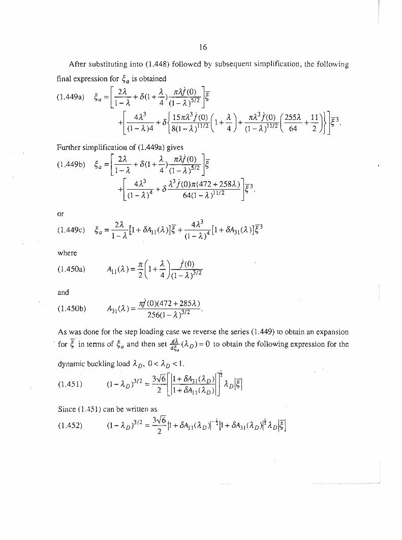
After substituting into (1.448) followed by subsequent simplification, the following
final expression for 5, is obtained
Further simplification of (1.449a) gives
where
and
As was done for the step loading case we reverse the series (1.449) to obtain an expansion
for c in terms of 5, and then set &(aD) = 0 to obtain the following expression for the 4,
dynamic buckling load AD, 0 < AD < 1.
Since (1.451) can be written as

17
we see that .(1.45 1) or (1.452) is useful with respect to 6 only for
61~31 (AD 11 CC 1, 61~11 (AD 11 CC 1.
By way of recapitulation, we note that we have been able to calculate analytically the
dynamic buckling load of the column subjected to a slowly varying time dependent loading
Af (6t). The result is shown in (1 .MI) and (1.452). As would be expected, (1.451) or
(1.452) reduces to (1 X I ) for the case f (6t) = 1 and b = 1 which is the step loading case.
We note that the result (1.451) or (1.452) holds irrespective of the particular slowly
varying loading function f (6r) provided f (6t) satisfies f (0) = 1 and 1 f (&)I c 1 for t > 0.
We similarly observe that up to the order E36, the dynamic buckling load ID of the
structure depends only on f(0) and that the load degradation is of the order 3 of the
imperfection parameter c. Hence a small imperfection of magnitude can give rise to a
large scale reduction in the buckling strength of the structure.

CHAPTER TWO
DYNAMIC BUCKLING OF A CUBIC MODEL - SPECIAL CASES
This chapter is devoted to determining the dynamic buckling load of the imperfect cubic
model for two separate cases, 6 = F and 6 = F2. We note that a general Taylor series
expansion of Sin terms of 5 takes the form
(2.001) 6 = S, + 45 + 6,c2 + ... It is however to be noted that 60 = 0 because 6, being a small parameter, must tend to zero
as F tends to zero. We note specifically that the two separate cases 6 = 5 and 6 = f 2
cannot be accomodated in one simultaneous treatment using (2.001) because when 6] z 0,
the linear term 45 in (2.001) dominates and thus the quadratic te,m 62F2 would not show
upin the asymptotic result. The quadratic term 62c2 dominates only if 6, = 0. We shall
however not extend the analysis beyond the quadratic term in because the contribution to
the dynamic buckling load from terms higher than the quadratic will be insignificant to the
order of approximation retained in the analysis.
2.1 Determination of the dvnamic buckling load of the imperfect model structure for the -
case 6=5.
The differential equation satisfied by the model structure was obtained in (1.105a). In
that case, the imperfection parameter F was not related to &and the dynamic buckling load
can be calculated from (1.45 1) or (1.452).
In the present case, we demand that 6 = f and the differential equation becomes
(2.1013) (+{I -af(St)}< - t3 = af(ft)S, t > o

19 d
where (') .= -() andb has been set equal to unity. dt
We introduce a new time scale and write
(2.101~) dtl - 1 - - dt -af(c.rl))K
where -
(2.101d) zl = { t
d We shall let ()' = c().
We substitute (2.102) into (2.101a) and (2.101b) and obtain
We now expand 5 in powers of 5 namely
We next substitute (2.104) into (2.103) and equate like terms and so obtain the following
The associated initial conditions are
(2.106a) u(')(o,o) = 0 for all i,

etc.
We now solve the problem (2.105). The solution of (2.105a) is
(2.107a) dl)(tl, q ) = yl(q)co~tI + B,(q)sin tl + A(?)
where
Using the initial conditions (2.106a, b) on (2.107a). We get
(2.108) -a
--A (0); 8, (0) = 0. y1(0)=-- 1-il
We now substitute into (2.105b) and get
+'ilft(l- yl sint, + 6, cost, 1. 2
where ' denotes differentiation with respect to the arguement.
To obtain uniformly valid solution for d2) in terms of tl, we equate to zero the coefficients
of cost, and sin t1 on the right hand side of (2.109) and so obtain
and
We solve (2.1 10) using (2.108) and get
(2.1 1 la) O1(.sl) r 0

Therefore
(2.1 12) U ( ~ ) ( ~ , . T ~ ) = + A(7 , )
The solution of (2.109) then gives
(2.1 13) ~ ' ~ ' ( t ~ , ~ ) = y 2 ( ~ l ) ~ o ~ t l + ~ ~ ( r ~ ) s i n t ~
The use of the initial conditions (2.106a.c) gives
(2.1 14) y2 (0) = 0, $2 (0) = -(I- ( ~ ' ( 0 ) + yi(0))
= -Af '(O)(4 - A ) / 4(1-
We now substitute (2.1 12) and (2.1 13) into (2.10%) and simplify to get
(2.115) MU(^) = -2(1- ~ f ) - l I ~ (- y; sin t, + e; cost, A +rf'(l - y)-312(-y2 sintl + e2 costl)
-(I - ajy-l(-y;costl + A")+ (1 - aj)-I - y: C O S ~ , I: To ensure a uniformly valid solution for uO) i n terms of t,, we equale to zero the
coefficients of sin tl and cost, in (2.1 15) and get
The solutions of (2.1 16) using (2.1 14) are
(2.1 17a) 1 e2(r1) = -(1 - if)-114 1:' (1 - /~f)-"~[y;r+ 3 y1 (f y: + ~ ~ ) ] d r 2

Thus (2.113) becomes
(2.11 8) ~ ( ~ ) ( t , , q ) = e2(q)sintl
We now solve for u ( ~ ) and get
(2.119) ~ ( ~ ) ( ~ , T ~ ) = y ~ ( ~ ~ ) ~ 0 s t ~ + 6 ~ ( q ) s i n l ~ - ( l - ~ f ) ~ ~ ~ "
with
The determination of the dynamic buckling load requires calculating the maximum
displacement
((la) ((tla,rla;C)
where t, is the particular value o f t where 4 attains a maximum. Thus at the maximum
displacement we expect
where tla and zla are the particular values of t, and zl respectively, where the maximun~ is
attained.
Using (2.121), we get - -2 -3 (2.122) -( yl sin t,, + ( 6, cost,, + ( [- y3 sin tla + 6, cost,,
3 3 sin 2tla + - yl sin 34, + C(1- Af )-'l2[C( yi' cos tla + A') 32
where each function of zl is evaluated at z,, in (2.122).

We expect the following Taylor series expansion to apply
(2.1 23a) ra = To + 57, + F2T2 +-.- -
(2.123 b) ria =i,+{il+F2i,+- -
(2.1 23c) 7,. = { ~ , = ~ ( T ~ + ~ T , + ~ ~ T ~ + . - - )
By finding a Taylor series expansion in (2.122) of each function of rI, about to each
function of zla about zero and thereafter equating to zero coefficients of 5 , we get
(2.1 24a) sin io = 0
This implies, to = nx, but taking n = 1, we get
(2.124b) A
ro = x
If we equate to zero the coefficient of f 2 we get
(2.124~) yl (o)?, - e2(0) + (1 - 2)-lt2{-y;(o) + ATO)) = o
In (2.124c), we have written down only the non-zero terms.
Thus, we get, from (2.124~)
we note, from (2.101~) that
(2.124e) tla = ~ k [ l - Af(fr)]dr
This simplifies to
The application of (2.123) in (2.124) gives
We shall now calculate the maximum displacement of the structure but however recall that
(2.125) {(I,, 7,; 5) = ~ ( * ) ( t ~ , ~ ) f + d2)(t1, r1 ) f2 + d3)(t1, 71)f3 + 0(f4).

substituting t la and q, for t1 and zl respectively.
By performing a Taylor series expansion of the series of maximum displacement for
each function of t,, about r and each function of zla about zero, regrouping according to
the coefficients of powers of 5 and thereafter writing down only the non-vanishing terms,
we obtain the maximum displacement 5 , of 5 in the following form
On evaluating each of the terms, we have
Further simplification of (2.126) gives
We note that generally we can write (2.126~) in the form
- -2 where cl , q and c3 are the coefficients of 5 , 5 and c3 respectively. We now reverse the
series (2.127) and have
(2.128) 5 = elto + e2t2 + e3t3 + - . a .

By substituting from (2.127) into (2.128) and simplifying we get
At buckling, we expect that there is ID such that &(AD) = 0. This implies 4,
(2.130) el + 2el{, + 3e& + ..-= 0
where (2.130) is evaluated at A = AD.
On simplification, we get
From (2.126~)
where
Therefore we have
Similarly we obtain
where
We also obtain
where

~ h u s using (2.13a-g) in (2.139) we get
We note that 5, is evaluated at A = AD. We shall however take the negative sign where the
square root occurs in the expression for 5, the reason being that the negative sign
automatically corresponds to the known step loading result if we set f'(0) = 0 and
f "(0) = 0 in the final expression for load degradation.
Now, from (2.128) we get
(2.133a) 3 5 = 5. + ~ 5 : )
But from (2.130), we have
(2.133b) 0 = (a(e1 + 2e25a + 3e35:)
Thus we obtain
The application of (2.132h) in (2.133~) taking into account the negative square root where
it occurs in the expression for {, gives
By way of recapitulation, we note that
(a) equation (2.134) gives a statement whereby the dynamic buckling load AD can be
calculated,

(b) equation (2.134) shows that, like the step-loading results ((1.305) and 1.321 for
b = 1) and the case where Sand are not related ((1.452)), the load degradation is 2 of order Tof the imperfection parameter f
(c) unlike the case where Gand 5 are related, the dominant expression for the dynamic
buckling load depends on f '(0) and also on f "(0)
(d) if we substitute f '(0) = f "(0) = 0 in (2.134) we obtain
This gives the result expected of a step loading case. This result is very much expected.
2.2 Determination of the dvnamic buckling load of the imperfect model structure for the -
cases=p
In this case the differential equation satisfied by the model structure is
(2.201 a) ( + {I - A . (c2r)}{ - 5 ) = AFf(C2r), r > 0
where (') = $0 and b has been set to unity.
We shall let
(2.202a) 4 = F2r
where
(2.202~) ~ ( q ) = f ( T t )
Thus we get
(2.203a) e = (1 - AF)~I~{, , + c15,,

where 0' = 4 0 . d72
We now expand ( in powers of and so write 00
(2.205) 50) = ( ( f2 ,4)= i= 1
We now substitute (2.205) into (2.204) and equate coefficients of like terms to get
(2.206a) AF ,@) ~ ( 1 ) + ~ ( 1 ) -
'2'2 I - AF
etc. The corresponding initial conditions are
(2.207 a) v(~)(o ,o)=o, j = 1 , 2 ,...
(2.207 b) v , ~ o , o ) = ~ , ( ~ ) ( 0 , 0 ) 2 = 0
(2.207~) l p ( 0 . 0 ) + (1 - I ) -~~ 'v~)(o ,o) = 0
etc. The solution of (2.206a) is
(2.208a) ~ ( ~ ) ( t ~ , . r ~ ) = yl,(r2jcost2+ ql(q)sint2 + D where
AF D=- 1 - A F
Using the initial conditions we get
(2.208b) y1 (0) = -D(O). I 0) = 0.

Since (2.206b) is homogeneous with homogeneous initial conditions we have
(2.209) ~ ( ~ ) ( t ~ , r2) = 0
We substitute into (2.206~) and get
(2.210) 5+$'0) = -2(1- IF)-"^ (- tyi sin t2 + q$ cost2)
To ensure a uniformly valid solution for v ( ~ ) in terms of t2, we equate to zero, the
coefficients of sin t2 and cost2 in (2.210). This gives AF'
(2.2 1 1 a) '; - 4(1- IF) - -3 ql (1 - AF)-"~ [D2 + l ( vf + $ )] W1 - 4
and AF' 1
(2.21 1 b) " - 4(1- AF) ql = 3 yl (1 - ~ F ) - " ~ [ D ~ + -( + $11.
4
Explicit determination of vl (r2) and q1 (22) is not necessary. We simply need y1 (O),
v;(O) and q1 (0) and qi(0). It is to be noted that tyl (0) andq (0) have already been
determined in (2.208b).
From (2.21 la) we get
From (2.21 I b), we get
On solving for ~ ( ~ ) ( t ~ , r2), we get

We note that
The use of initial conditions on (2.21 3) gives
So far the equation for displacement becomes
(2.216) 5(r2,z2) = 5 ( y l cost2 + q1 sin12 + D)+ f3[y3cost2
1 +- (3 W:'ll - $)sin 3t2 + yl ql D sin 2r2 32
We shall now determine the maximum displacement, {,, in order that the dynamic buckling
load, AD, be evaluated.
d 5 At the maximum displacement, there exists t = tc such that T(tc) = 0. We shall let
t2, and r2, be the values of r2 and z2 respectively at r = t,. We let r2, and z2, be
expanded in the following Taylor series
(2.217a) f2c = I f ) + ti2)52 + t/2)53 + . . . (2.217b) -2 -3 tc=t0+t2{ +t35 +"' (2.2 17c) = c2b = f2(to + t2c2 + t3F3 + . -)
d 5 Requiring that -;i;-(tc) = 0, implies from (2.203a) that

The substitution of (2.216) into (2.21 8) gives -3 (2.219) ~ ( - y ~ s i n r 2 c + q l ~ ~ ~ t 2 c ) + ~ [ - y 3 ~ i n 1 2 c + t l j ~ ~ ~ t 2 c
We note that every function of 72 in (2.219) is to be evaluated at 72 = z2,.
Next, we expand each function of t2c and 72c of (2.219) in a Taylor series expansion
about (t2c, rZc) = ((j2),0) and equate to zero like cofficients of 5 and obtain
(2.220a) sin ti2) = 0
This gives
(2.220b) tL2) = nz, n= l , 2 , .... We shall however take n = 1 for definiteness. Therefore we get
(2.220~) p) 0
Similarly, we obtain
where to is evaluated in a manner similar to the determination of To in (2.124g) and in fact
has the same value as To which is --"-- By expanding each function of t2 and z2 of (I -A) ' '~
(2.216) in a Taylor series about (r2,r2) = (rA2),0) and thereafter collecting terms in powers
of 5 , we obtain the maximum displacement 6, of 6 in the following way r

Further simplification of (2.221) gives
By performing an analysis similar to the one used from (2.127) to (2.134) we'see that at
buckling
where cl and c3 are now evaluated at il = AD.
From (2.223) we get
where
f ' ( 0 ) = F'(0).
The following salient points are to be noted.
(a) The dynamic buckling load for the case 6 = f can be calculated from (2.224) 2
(b) The load degradation is of order 7of the imperfection parameter 5.
(c) The dynamic buckling load in this case depends on f '(0).
(d) For f '(0) a 0 the result (2.224) gives the step loading result which is
(2.225) ( 1 ~ ~ ) ~ ~ - 36 D I 51 2
(e) We conclude that, in general, the dynamic buckling load of the imperfect cubic
structure depends on 6 and c. If 6 and 5 are related linearly, then the dy narnic
buckling load is evaluated from (2.134) whereas if there is a quadratic relationship

33
between them in the form 6 = F 2 , the dynamic buckling load is evaluated from
(2.224). These two results, are not equal unless in a situation of step loading.
(f) The results (2.224) is asymptotically equal to that obtained from (1.451) if in the
latter we replace 6 by F 2 .

CHAPTER THREE
DETERMINATION OF THE DYNAMIC BUCKLING LOAD OF A SPHERICAL CAP
SUBJECTED TO A SLOWLY VARYING TIME DEPENDENT LOADING
fl Derivation of Equations
We shall consider a shallow section So of a spherical cap and take Cartesian coordinates
x and y in the base of the plane and z coordinate normal to this plane. We shall give the
membrane strains E,, E>. and E~ in terms of the tangential displacement U, V and the
normal displacement as W which acts in the radial direction. We shall similarly let K,, K,
and K~ be the components of curvature in the indicated directions while N,, Ny and Nxl
represent the stress components. The couple is represented in its component form as
M,, My and Mq. We emphasize that the suffices appearing in E, K, N and M above are
not to be interpreted as indicating differentiation. In static situation, all the above space
variables depend only on the spatial variables x and y while in the dynamic case, time is an
additional independent variable. The strains and curvature are given in terms of the
variables U, V and W as
&Y
(3.101) 1::

where expression such as W, indicates partial differentiation of W with respect to a.
Similarly, the stress-strain relationship is given by
(3.102)
where
E is Young's modulus and v and h are the Poisson's ratio and the shell thickness
respectively. As before, surfices following N, M, E and K in (3.102) do not indicate
differentiation.
For the classical static buckling analysis, we consider the case in which the strains,
stress and displacement are time independent and in which the spherical cap is considered
perfect. We shall let P be the time independent lateral pressure acting on the spherical cap .
Using calculus of variation and the principle of virtual work, we can derive the three
differential equations of equilibrium in U , V and W. If however, we introduce Airy's srress
function F ( x , y ) for stress resultants which gives
(3.103) Nx = Fyy, Ny = Fxx, Nxy = -Fxy
and finally take the variational equation given by
(3.104) j j [ ~ ~ 6 ~ ~ + My6rcy + 2 M , 6 ~ ~ + NX6zx + N y 6 ~ y + 2 ~ ~ 6 ~ ~ ~ ] y l d ~
= external virtual work,
we obtain the following equilibrium equation

and the compatibility equation 1 1
(3.106) - V ~ F --V'W + W,Wyy -(w,,)' = 0 Eh R
where V4 and v2 are the two-dimensional bihlumonic and Laplacian operators
respectively. Before static buckling sets in the perfect shell is in a uniform membrane
stress state where
where R is the radius of curvature of the shell. For subsequent state, we take
where f and w are zero prior to buckling. The linear buckling equations are obtained by
substituting (3.108) into (3.105) and (3.106) and linearising with respect to f and w to get
(3.109) 1 1 D V ~ W + - V ' ~ + - P R V ~ W = O R 2
We obtain periodic solutions of these homogeneous eigenvalue equations by taking
Substituting (3.1 11) into (3.109) and (3.1 10) gives
(3.112a) B = - ~ h ( ~ , ~ + gy2)-1
(3.1 12b) 2Eh
P =-[(gx2 R +gy2)-I + ~ ~ ( g ~ ~ + gy2)]

where '
and suffices in g, and gy do not indicate differentiation. To find the critical buckling load
PC, we minimise P with respect to g, and gy and obtain
(3.1 13) g? + gy2 = e2 as the condition for the attainment of the critical load PC. For the condition (3.11 3), the
critical pressure PC becomes
The dynamic equi!ibrium equations for the case of an imperfect spherical cap subjected
to step loading was similarly obtained by Danielson [8]. His work was in turn based on an
earlier work on static buckling of an imperfect spherical cap by Hutchinson 191. In this
case, the stress-strain relation and displacement now depend on both the spatial variables x
and y as well as on time t . The displacement of any point on the spherical cap was taken by
where Wo is the prebuckling radially symmetric mode, W, is the axisymmetric buckling
mode and W2 is an arbitrary non-axisymmetric buckling mode. The imperfection was
taken (by Danielson) in the form
(3.1 16) W = @$ + F2w2. In a manner similar to the derivation in the static case [7,8,9], the following multiple mode
dynamic equilibrium equations were derived for the step loading case, where t > 0

where A is the "amplitude" of the applied step load and K~ and K2 are scalars. It is to be
noted that 5; << 1, z2 << 1 and o O , w, and w, are the circular frequencies of the
prebuckling and axisymmetric modes and the circular frequency of the non-axisymmetric
mode respectively all of whose numerical values are embodied in the derivation of (3.1 17)
[BI .
3.2 Solution of the Problem -
For our problem we shall determine the dynamic buckling load of an imperfect
spherical cap subjected to a slowly varying time-dependent loading, where the time
dependent loading is taken in the form Af (St) and f (0) = 1, 1 f (&)I < 1, t > 0, S c< 1.
The modification of (3.1 17) to this new problem gives
An analytical solution of (3.201) will now be sought for the case in which the prebuckling
wme number wo is infinitely large. This would also be the case if we set the prebuckling
inertia term to be iero i.e.
This then means that
(3.203) to( t> = Af (61)

Hence,'from (3.201), we get
In (3.204) we have already asserted that f = f (6r). For our solution we shall set 5, = 0.
This choice is informed by earlier works [7, 81, that lower values of dynamic buckling
loads (for step loading case) are oblained if is numerically set equal to zero. We expect
this to be true for our case since step loading is a particular case of slowly varying loading.
The analysis to be presented here will follow the following procedures.
Calculating uniformly valid expressions for the displacements of the two buckling
modes t1 and t2 since that of to( t ) has already been known as in (3.203),
finding maximum displacement for each of these modes and hence evaluating the
effective maximum displacement for thz whole spherical cap,
reversing the series for effective maximum displacement,
determining the dynamic buckling load and
making pertinent deductions from the rzsult obtained in (d).
We shall let
In the analysis to follow, we shall l e ~ I I'.
We now generalize the Lindstedt-Poixare method by defining i by

Then we have
where n = 1,2 and henceforth, partial differentiation with respect to t and z such as
6,- and tnr, shall not be indicated with the use of a comma.
Thus we get
We substitute (3.207) into (3.204a) and get
where we have used the fact that 5 - 0.
By substituting (3.207) into (3.204b) for the case n = 2, we can derive an equation similar
to (3.208a) for t2. We shall let 6, and t2 be expanded in the following double series.

where aik = a"(;, z) and bir = bir(;, T) and the superscripts appearing in aik and bjr are
understood not to be powers. By substituting (3.209) into (3.208) and equating both - i k coefficients of 5 6 and F i g r (at the respective appropriate instances), we have the
following sequence of equations:
(3.210b) ~ a ~ ' = -2 ~ ~ ( 1 - Af ) - 112 20 - 1 A ) a;,
etc. The initial conditions for are
(3.2 1 1 a) a2k(0,0) = 0 for all k .
(3.21 1b) aY(0,o) = 0
etc.

The initial conditions for bir are
(3.213a) bjr (0,0) = 0 for all j, r,
(3.213b) bi O (0, 0) = 0,
(3.213~) bi '(o,o) + (1 - A)-112 b:' (0, 0) = 0,
0 2
We have not included ~a~~ and Lb2' because calculation shows that a3k and b2' ( k , r
= 0, 1, 2, ...) are numerically zero.
We first solve (3.212a) and obtain
t 3.214a) b1'(?,r) = alO(r)cosi +p,,(r)sini + B ( r )
'The use of initial condition (3.213) on (3.214a) gives
t 3.214~) alo(0) = -B(O), PI&> = 0.

We now substitute (3.214a) into (3.212b) and obtain
~ b " = - 2(1- (3.2 15) (- aio sin i + &'o cos i)
0 2
+ y'(1 - af )"I2 (-alo sin i +fro cosi)
202
To ensure uniformly valid solution for b1 in respect of i , we equate to zero the
coefficients of cost and sin i in (3.125). This gives respectively
The solutions of (3.216), bearing in mind (3.214~) are
(3.217b) Plo(z) e 0.
Thus, we obtain from (3.215)
(3.2 18a) bl'(i,z) = all(z)cosi +a1(z)sini .
The use of initial condition (3.213) on (3.218a) gives
Next, we substitute (3.2 l4a), (3.21 8a) into (3,.212c) bearing in mind (3.217a) and
(3.217b) and get
(3.2 19) 2(1- A , ) - ] / ~ (-ail sin i + pil sin i)
0 2

To ensure uniformly valid solution for bI2 in terms of i , we equate to zero the
coefficients of cosi and sin; in (3.219) and obtain respectively
and
The solutions of (3.220), bearing in mind (3.218b) are
and
(3.221 b) a,,(O) EO.
We now solve for bI2 in (3.219) and obtain
(3.222) (1 - ~f )-I B"
bI2(i,r) = a12(r)cosi +PI2(r)sini - 4 On using (3.213), we obtain from (3.222)
So far. we obtain
(3.2243) blO(i, 5) = a l 0 ( ~ ) c o s i + B(5)
(3.224b) b 1 ' ( ~ , ~ ) = / l l I ( ~ ) s i n f
Further analysis gives
(3.224~) b12(i, 5) = a12(r)cosi - (1 - 2f )-I B"
4 We note that, using (3.224a),

Substituting (3.225) into (3.210a), we obtain
Thus, we solve for a20 in (3.226) and obtain
. (3.227a) a20 (i. 7) = ( r ) c o s ( ~ ) i + ty(r)sin(%)i 6'2
r
The use of initial conditions (3.21 1) on (3.227a) gives ,-
We note the following, using (3.224a,b) 1 0 1 1 1 (3.228) b b = - aloP1 sin 2i + BPl sin i.
2
Thus, substituting (3.228) into (3.210b), we obtain
(3.229) ~ a ~ ' = - - ~f [(: 1 - - ei0 s in(z ) i + ty;o co s (5 ) i ) a 2 w2
#
-[(l-~f)-la?o] sin2i 2Ba1,(l-)if)-1sini 2
- 2 (2) - 4 (2) - I

To ensure a uniformly valid solution for a2' in terms of i , we equate to zero, the
coefficients of cos($)i and sin(%);. This gives
and
(3.230b) a f y i - af)-312
202
Since (2) + 0 , we solve (3.230) bearing (3.227) in mind and obtain
We now solve for a2 ' ( i , T ) in (3.229) and get
(3.232) n2'(i,r)=821(r)~~~(~)i+y21(r)sin(~)i r
2
- ~2 (2) ( 1 - af )"I2 2Balo sin
202

Using the initial condition (3.21 I), we obtain
(3.233a) (0) = 0
where (3.233b) is evaluated at z= 0. A detailed simplification of (3.233b) gives r

We note that, using (3.224), the following simplification holds:
We now substitute (3.224b), (3.234), (3.232) and (3.227a) into (3.210~) and get (using

a& cos 2i + 2Ba10 cosi
4 {(%i'-I} I To ensure uniformly valid solution for a", we equate to zero, the coefficients of
cos($)i and sin(?); in (3.235) and obtain
The solutions of (3.236), using (3.233) are 114
(3.237a) ylzl(7) = y1,l
(3.237b) 92, (z) 0
22 - We do not need the explicit determination of a ( t ,z) in this work. So far, we h~ivt:
obtained the following
+- I a', cos2i + 2B:10 cosi 2 2 ) - 4 3
r 1

2 B q o sin i +
I 2Wa1o(l- ~f
aloj311 sin 2; BPll s in i 2{($r - + {(g -
+
K ( 1 - A - 1 alo 2 sin 2i
As indicated before, a3j ( i , r ) r 0 V j. We now note the following multiplication:
' - 1 1 2 202 i{(?r -4y
Substituting (3.240) and (3.212d) in (3.212d), w e get 2
(3.141) ~ b ~ ~ = - ( I - ~ f ) - " ~ ~ j a , ~ c o s ~ - ( l - ~ f ) - ~ 6'2
2 +cos(i - W. . + B&, cos (2 ) i - {(a) aIo q ( 1 - ?J)-'

cost
- 3 a&8(1- Af )-' cos 2 i 3{2jZ~2{($)2 }
To ensure a uniformly valid solution for b30 in terms of i , we equate to zero the
coefficients of cosi in (3.241) and get
Thus, we get r
We now solve for b30 in (3.241) and get

The use of initial condition (3.213) on (3.244) gives -
We note that the expression on the right hand side of (3.245a) is to be evaluated at z = 0.
A further simplification of (3.245a) yields

We now note the following multiplications
[("+ 2 B ~ ) ~ ~ .in; + a&pl (sin 3i - sin i ) B& lalo sin 2i 4 { Q 2 - 41
+ w, 2 ( ) -1 I
2 + sin i) B P I , sin 2i - 2 ) a lo t l - .~f +

aloj31 sin 2; BPI, sin i . 2 J. 2 - 4 + 1 - I}
We now substitute (3.224a,b), (3.244), (3.246a) and (3.246b) into (3.212e), usins
(3.246) and obtain 2 2
(3.247) ~ b ~ ' = -(l - ~f )-1'2p;~l sini +=(I - ~f ~ f ) ' ' ~ j a ; ~ sin i 0 2 6'2
W - W 2 W, 2 ((1 - ~f I-' ~ e ~ ~ ) ' + n ( k ) t ((-) ~ ~ a : ~ ( l - . z . ) - * ) ~ ( ( ~ ) - 3) +
W, 2 + O2 sin 2t
1 - (& W , 2 0, 2 { - { - 4)
W 2 3($) K2 {a:o (I - Af)-2)'sin 3i + - a 3 ~ sin i 32{(2)' - 4)
+p30 cos i + (2 - 3

a:o(sin 3; + sin i) Bat, sin 2; 2 +
6) 2 {(a) - 4) {Q2 - 1)

{[*+B2hl1sini+ a:op, , (sin 3 i - sin i) + BP] 0, ,alo 2 sin 2; ( 1 -1
To ensure a uniformly valid solution for b3' in terms of i , we equate to zero the
coefficients of cosi and sin ; in (3.247) and obtain
The solution of (3.248a), using (3.245b) is
(3.249a) P30(~) = O .

We now solve for b31 from (3.247) and get
01 2 0 2 - ( ) 2 1 - ) 2 ) ' { ( ) - 3) sin 2i
W, 2 6'1 2 3{(q) - } { - 4)

aloPl, sin 3; B& sin 2; + 32{( 2)2 - 2) 6{(?)2 - 1)
Using the initial conditior. ('3.21 3), we get from (3.250)
(3.25 1 ) a3,(@. = 0


60
We shall now expand in a Taylor series about (id1),0;5;,6). Carrying this out. we
where each aV in (3.255a) is to be evaluated at (iil), 7:)) = (iA1),O).
-(a (2) In a similar way, we expand e2. in a Taylor series about (to , z, ) = (d2),0) and gel
(3.255b) 52. = F[b1' + ~(b:';;? + bi0tA2) + bl1]
-3 1OA(2) lb t + 1On(2) 10 (2) +< [bi tzo + ;;;(;I bm + s{+ t21 + b, t2(,
respectively, that at maximum displacement for el and 52 , we expect to have
(3.256a) - ( d51 ( I ) )= ~ ~ ( l - ~ f ) l ' ~ < ~ ~ + (&c2 +/ljf; +. - - ) t l i + 6elr = O dt
and
When the right hand sides of (3.256a) and (3.256b) are to be evaluated at (i, z) = (iL1), rill)
and (i, z) = (fi2), rL2)) respectively. Now (3.256a) implies, using (3.255a), that
-(2) (2) where (3.256~) is evaluated at (f, z) = (I, , z, ). We now expand (3.256~) in a Ta!,lor
-(l) (1) series about (fa z )=(iA1).O) bearing (3.252) in mind and then equare to zero the
-2 j coefficients of 5 6 in order to satisfy (3.256~). From the coefficient of (c2,1), we gsi

From the coefficients of ( f2 , 6 ) , we get
(3.257b) a?!i(l) rl 01 + + rr 0 + (1 - ~ ) - ~ 1 ~ ~ : ~ = 0
( 1 ) where n2j , j = 1,2 and their partid derivatives are evaluated at ( t , , ra ) = (;A1),0).
Solving (3.257a) using (3.238), we get - -
I afo sin 2ii1) 2 a l o sin iil) (3.258a) (2) rc2 (1 - Af 1-l @, +
0 2 - o~~ (0) sin(2)ih1) = 0. - 4 - 1
Similarly, from (3.257b) and using (3.238) and @.239), we get
(3.258b) + + (1 - 1)-"2 a:0]
The expression (3.258) so far being evaluated at ( i i l ) ,r i l ) ) = ($),o). We note the
following simplifications
( 3 . 2 5 8 ~ ) a ~ ~ ( i h l ) , ~ ) = - ( % ) ~ ~ o ( ~ ) s i n ( ~ ) i ! l ) wz 0,
-

Further simplification gives the following:
where
and

The use of (3.258) will enable fit) to be determined for specific values of ;A1) found from
(3.258a). We similarly determine a2' (fil),O) and obtain r r
We shall however represent u ~ ~ ( $ ' ) , o ) simply as
where A1(&,fd1)) and A2(3,id1)) are defined in an obvious manner from (3.258j). The 0 2 0 2
evaluation of ty2' (0) gives r 1
We next evaluate U ~ ~ ( ; ~ ( ' ) , O ) and get
3 f cos 24') 2 cos id1) -{-+ 0 1 2 - 2 ( ) - 4 ( 3 ) 2 - 1
6'2 0 2
Thus, following (3.255a) and (3.258), we obtain cl, as:

In deriving (3.259), we have used the fact, following (3.257a) that ay(;f),0)= 0 .
We are yet to determine t i 1 ) in (3.259).
We next expand (3.256b) in a Taylor series about (i,(2),e))= (fh2),0) bearing
(3.255b) in mind and equate to zero coefficients of 5d6' (j = I , 2 ,...; r = 0, I , 2 ,... ).
From the coefficient of (c2,1), we get
(3.260a) 10 (2) 0) = 0 b; (fo 9
This means
(31260b) -al0(0)sin id2) = 0, ;A2) = nn, (n = O,1,2, . . .). We shall however take n = 1. Hence we get ;A2' = n.
By equating the coefficient of 58, we get
(3 .'260c) '0 -(2)b10 ii + 0 p)b!0 17 + b! I 1 - (1 - A )- 112 br 10 = 0
where (3.260~) is to be evaluated at (iL2), rL2)) = (n,O). This gives
If we equate respectively the coefficients of ( g . 1) and ( C S ) , we get
(3.260e) -(2) = -(a = 0 '10 '11

By equaring the coefficient of (::,I), we get
With (3.260) in mind, we now rewrite (3.255b) with only the non-vanishing terms thus 3 30 (3.26 1 ) = C2[b1O + bi0tA2)6 + . - a ] + t 2 [ b + 6(b:'t$;) + b ~ ~ f ~ ~ ) ? ~ ~ )
where bjr and partial derivatives are evaluated at (iA2),0) = (z,O) in (3.261). We shall
now evaluate each of the terms appearing in (3.261). Thus from (3.249~) we get

If we substitute into (3.262a) we get the following lengthy result.

We also evaluate the following at zo = 0:
Thus, we have
If we substitute for a;o(0) from (3.262j) we get
where

We now evaluate from (3.250) and get after simplification
where
From (3.244) we get
Thus, using (3.260d), we now evaluate b:0(ii2),0)?$2) and get:

where ~ ~ ( 3 ) represents the terms inside the square bracket of (3.266e). Using (3.218b) '"2
and (3.2600, we evaluate b:' (iA2).0)$i) thus
(3.266e) by (?h2.0)?$) = K 3 { - 2
4u2(1 - -1 * - 4 ( ) 0, 2 -1 +I}. 2 '"a
Similarly we evaluate
where
From (3.244), we evaluate b30(fo(2),0) and obtain
where -

( 2 ) We shall now evaluate t f ) , t i 2 ) and t20 .
From (3.206a), we get (4
1.
(3 .267) ca) = w J (I - 2f (6ts))ll2 dts
Using (3.252), we get
112 ( 1 ) 112 ( 2 ) 112 ( a ) (3.268a) f 1 = 1 -A) to , ih2) = a2(1 - 2 ) to , iit) = u 2 ( l - 2 ) t20
Using (3.206b) on (3.268a) we get
- 1 = - 1 = 1 112 ( 1 ) '0 '0 2 ( - 2 ) to .
' Therefore
Similarly, we obtain
Using (3.268a), (3.206b), (3.243) and (3 .260f) , we get
112 ( 2 ) g = a ( I - A ) t20 + pi (0 )
from which we evaluate
where

dynamic stability of the structure at this stage. This is essentially the main
conmbution from our first level of approximation (3.281a). Thus, strictly speaking,
as far as the initial post buckling is concerned, the coupling term plays no part.
This means that at this stage the coupling term can be neglected in the problem
compared to ~ ~ 5 : This is an important result that has never been obtained before.
(vii) (3.288) is certainly a "refinement" of (3.284) and clearly shows the contribution of
the coupling term 5,<2 on later post buckling phenomenon.
(viii) As the results (3.284) and (3.288) show, it is possible in this problem to relate the
dynamic buckling load AD under slowly varying loading to the static buckling load
As and thus by-pass the labour of repeating the calculation for various imperfection
parameters. This is done by noting that the static buckling load As of the spherical
shell (with Kl<? neglected) is given by
(4.01) 3
(1 - 2,)' = 2&JF& If we eliminate I&/ from (3.284) (a similar procedure can be done for (3.288)) we get
I + fif'(0) m. -(I) (I) A3(-,fO ,to .
4(l- A D ) @2
-(1) (1) ( t o t o ) is evaluated at a = I D .
If we set f'(0) = 0 in (3.284), (3.288) and (4.02), we get the following results
corresponding to the two levels of approximation in the step loading case:

sin sn
Evaluating b:Ot$g) at (fi2),0) = (z,O), we get
Let
(3.2680 G9 (s) = AGl (s) + G2 (s)
Then
We shall further let
(3.268h) sin sn.
Then, we have by(fd2),0)f$) as
We now assemble all the individual terms in (3.261) (which have been evaluated) anti
determine the maximum displacement c2a for r2. The result is
+(I - +)G* + 2 ~ , - 6, + c3} + 0(2j2)]
where we have, for simplicity, deleted the dependence of G: on 5. We note that, from 0 1
(3.259), the corresponding maximum displacement for 5, can be rewritten as

(3.270)
where
(3.27 1)
K 2 ( 3 2 ~ 2 n [{ - 2 i ( l )
5'; = - ~ ) 3 w 2 "I 2 +- cos-
0, } O (A) - 4 (y) -1 2
On account of (3.203), we see that the maximum displacement for the prebuckling
mode gc! is
(3.272) jOa = A
Now, following (3.1 15), the effective maximum displacement for the spherical shell is 5,
and is given t.1
Using (3.2691. (3.270) and (3.272), we get

+(I- 4)G8 + 2G7 - 7rG9 + G3}].
It is to be emphasized that for any allowable choice of 2, iil) must necessarily satisfy
We shall now determine the dynamic buckling load of the imperfect spherical cap
subjected to a slowly varying time dependent loading. We shall however give the results in
two separate levels of approximation. It is anticipated that each of these results will
automatically establish some far reaching consequencies.
We now write the following
Following (3.274), we recast (3.273b) in the form
We shall for simplicity write (3.275) as -
(3.276) 6 , = 2 + d 1 t 2 +d2c22+d3c2+...

On account of (3.203), we see that the maximum displacement eOa for the prebuckling
mode is
(3.272) 50, = 2
Now, followi~g (3.115), the effective maximum displacement for the spherical shell is 6 ,
Using (3.2691, (3.270) and (3.272), we get
(3.273b) C
I-A 8(1-
74
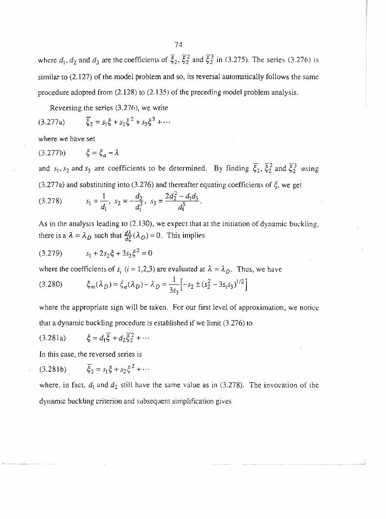
where dl , d2 and d3 are the coefficients of c2, 5: and 5: in (3.275). The series (3.276) is
similar to (2.127) of the model problem and so, its reversal automatically follows the same
procedure adopted from (2.128) to (2.135) of the preceding model problem analysis.
Reversing the series (3.276), we write
(3.277a) c2 =sl( + s 2 t 2 +s3t3 +- - -
where we have set
(3.277b) 6=5,-a and s1, s2 and .Q are coefficients to be determined. By finding f2, c: and using
(3.277a) and substituting into (3.276) and thereafter equating coefficients of 5, we get
As in the analysis leading to (2.130), we expect that at the initiation of dynamic buckling,
there is a a = AD such that $(AD) = 0. This implies
(3.279) s1 +25& +3s3t2 = O
where the'coefficients of si (i = 1,2,3) are evaluated at A = AD. Thus, we have
,(3.280) 1
5,n(AD)= {,(AD)-AD =-[-s2 ?(s; - 3 ~ ~ ~ 3 ) ~ ' ~ ] 3x3
where the appropriate sign will be taken. For our first level of approximation, we notice
that a dynamic buckling procedure is established if we limit (3.276) to
(3.28 1 a) ( = d l c + d2f22 + In this case, the reversed series is
. (3.281b) & = s ~ { + s ~ ~ ~ + - .
where, in fact, dl and d2 still have the same value as in (3.278). The invocation of the
dynamic buckling criterion and subsequent simplification gives

where and are evaluated at 1 = AD. On evaluating (3.282), we get
(3.283) (1 - = ~ A D I K ~ ~ ( ~ ) 0, 2 11 + + 6f'(0))~1)I.
Further simplification gives
valid for Wl W1 1<-c2pc->2. 0 2 a 2
So far, (3.284) gives the result of the fust level of approximation. We shall now determine
the result of the second level of approximation. In this case we use (3.277a) - (3.280).
Using an analysis similar to the derivation of (2.133a) - (2.1 33c), we get
where the right hand side of (3.285) is evaluated at 2 = AD which is the dynamic buckling
load sought. We shall now evaluate each of the terms in (3.285) and (3.280). Following
(3.275) and (3.276), we get
(3.286a) 2 1
dl = -(I + 6f '(0)Rll) I-a

Thus, we have
Thus, we have
The evaluation of 6 , from (3.280) gives
By substituting for 6 , in (3.285) and simplifying thereafter, we obtain the following
lengthy expression

where
0 1 0 1 Equation 3.288 is valid for 1 < - < 2 or - > 2. All functions of A in (3.288) are 0 2 0 2
evaluated at AD and we have taken the negative square root sign where root occurs, this
choice being informed by the same reason leading to the determination of (2.134).
CHAPTER FOUR
DISCUSSION OF RESULTS
The results (3.284) and (3.288) give the expressions for determining the dynamic
buckling load AD of the spherical cap. In either case, we see that the load
degradation is of order 5 of the imperfection parameter 5;. The dynamic buckling load AD depends, among other things, on the ratios of the
circular frequencies of the buckling nodes and t2 except hat 2 # 1.2.
The two results (3.284) and (3.288) hold with no additional restriction on the slowly
varying time dependent loading function f (6t).
We observe that to order F36 in the effective maximum displacement (such as in
(3.273b), and generally to any nonlinear order in f2 (but linear in 4 in which
the effective maximum displacement of the spherical cap is determined, the
corresponding dynamic buckling load depends, as far as f (at) is concerned, on
f'(0). If however the determination of the maximum displacement is g i ~ e n to an
accuracy that is nonlinear in 6, the dynamic buckling load, in this case, will definitely
depend on f '(0) and on higher derivatives of f (7) evaluated at 2 = 0.
Up to the order c36 in the maximum displacement, there is no tacit dependence of
the two results (3.284) and (3.288) on the quadratic term ~ ~ 5 : and this confirms
Koiter's assertion [7, 81, that the term K~<: can be neglected compared to the effect
of coupling between the two nodes as far as initial post buckling behaviour is 1
concerned. I
I
The result (3.284) shows that to order c26 in the determination of the effective i maximum displacement, there is no contribution of the coupling term 5,:- . - on the i

The results (4.03) - (4.05) are novel derivations with possible applicability in
Engineering. They have long been sought for but never obtained analytically. The
only known analytical attempt is that in a similar work by Budiansky and Hutchinson
[2,4] in which they sought the dynamic buckling load of an imperfect cylindrical
shell subjected to step loading. The governing differential equation in this ciise is
equivalent neglecting the quadratic term ~ ~ e : , setting F, = 0 in (3.204) and setting
f(&) E 1. Budiansky and Hutchinson obtained approximate solutions by neglecting d'5 the inertia term --& in (3.204e). The approximate solutions are

from which it follows that
In what follows, we shall undertake a case study of (4.02) - (4.07) for 2 = ,I
112 (integer), v = 0.3 and k2 = &[3(1- v2)] . Table I summarizes the salient points.
From the Table 1, we make the following deductions:
In general, the dynamic buckling loads calculated from (4.06) give higher values
compared to the ones calculated from (4.03) and the disparity becomes greater with 0 increasing 1 . 0 1
The dynamic buckling load decreases with increased 2 and c2. The approximate values of dynamic buckling load AD = A I D , say resulting from
(4.06) can be several times higher than the values AD = A20, say, from (4.03) W 0 particularly when is very high. A I D is only comparable with j / 2 D when 2 is W2 %
exceedingly s~nall. -
For all values of t2 and 2 tested, the expression 6G5 . - 5 ~ ; b in (4.04) was "2
negative. We thus conclude that the coupling term 5,c2 does not necessarily lead to
buckling. Thus the structure still maintains its load carrying capability when the
influence of the coupling term t 1 j 2 is called to play. Thus, it is only the quadridtic
term that dominates initial post buckling phenomenon; does not. This result is
also true of (3.288).

REFERENCES
J.C. Amazigo, "Buckling of stochastically imperfect columns on nonlinear elastic
foundations", Quart. Appl. Math (1971), pp. 403-409.
B. Budiansky and J.W. Hutchinson, "Dynamic buckling of imperfection sensitive
structures", Proceedings of XIth Inter. Conm. of Appl. Mech., Springer Verlag, Berlin
(1966).
J.C. Amazigo and D. Frank, "Dynamic buckling of imperfect column on nonlinear
foundations", Ouart. Appl. Math, Vo1.31, No. 1 (1973), pp. 1-9.
B. Budiansky, Dynamic buckling of elastic structures: Criteria and estimates. In
Dvnamic Stabilitv of Structures, Pergamon, New York (1966).
J.D. Cole, Perturbation Methods in Applied Mathemati~, Blaisdell Waltham 1966.
J.W. Hutchinson and B. Budiansky, "Dynamic buckling estimates", A.I.A.A. J. Vol.
4, No. 3 (1966) pp. 525-530.
V. Svalbonas and A. Kalnins, "Dynamic buckling of shells: evaluation of various
methods", Nuclear Enpineering and Design, Vol. 44 (1977), pp. 331-356.
D. Danielson, "Dynamic buckling loads of imperfection-sensitive structures from
perturbation procedures", A.I.A.A. J. Vol. 7, No. 8 (1969), pp. 1506-1510.
J.W. Hutchinson, "Imperfection sensitivity of externally pressurized spherical shells",
J. Appl. Mech. (March 1967), pp. 49-55.
10 B. Budiansky and J.C. Amazigo, "Initial post-buckling behaviour of cylindrical shells
under external pressure", J. of Math. and Phvscs, Vol. 47 No. 43 (1968),. pp. 223-
235.

8 3
1 1 D. Lockhart and J.C. Amazigo, "Dynamic buckling of externally pressurized imperfect
cylindrical shells", J. Appl. Mech,, Vol. 42 (1973), pp. 316-320.
12 J.C. Amazigo, "Dynamic buckling of structures with random imperfections". In
Stochastic ~roblems in Mechanics, Ed. H. Leiphelz, University of Waterloo Press
(1974), pp. 243-254.
13 R.S. Roth and J.M. Klosner, "Nonlinear response of cylindrical shells subjected to
dynamic axial loads", A.I.A.A. J,, Vol. 2 No. 10 (October 1964), pp. 1788-1794.
14 J.C. Amazigo and D.F. Lockhart, "Stability under step loading of infinitely long
columns with localized imperfections", Ouart. ARD~, Math. (1976), pp. 249-256.
15 D.F. Lockhart, "Post-buckling dynamic behaviour of periodically supported imperfect
shells", Int. J. of Nonlinear Mechanics, Vol. 17, No. 1 (1982), pp. 165-174.
16 Y.S. Tamura and C.D. Babcock, "Dynamic stability of cylindrical shells under step
loading", J. Apwl. Mech. (1975), pp. 190-194.
17 C.A. Fisher and C.W. Bert, "Dynamic buckling of an axially compressed cylindrical
shells with discrete rings and stringers", J. Apwl. Mech. (1973), pp. 736-740.
18 M.C. Cheung and C.D. Babcock, "An energy approach to the dynamic stability of
arches", J. ADD]. Mech. (1970), pp. 1012-1018.
19 J. Arbocz and C.D. Babcock, "The effect of general imperfections on the buckling of
cylindrical shells", J . Appl. Mech. Vol. 36, No. 1, TRANS. ASME, Vol. 91, SERIES
E (1969) pp. 28-38.
30 G.F. Carrier, M. Krook and C.E. Pearson, Functions of a Complex Variable: Theorv
and Technique, McGraw-Hill, New York, (1966), pp. 61-62.


T A B U 1
Compar i son of t h e r e s u l t s 4.03 a n d 4.06
Result o f 4.06
1D
Result of '4.03
2D